Magnetoclinicity Instability

Abstract

In strongly compressible magnetohydrodynamic turbulence, obliqueness between the large-scale density gradient and magnetic field gives an electromotive force mediated by density variance (intensity of density fluctuation). This effect is named “magnetoclinicity”, and is expected to play an important role in large-scale magnetic-field generation in astrophysical compressible turbulent flows. Analysis of large-scale instability due to the magnetoclinicity effect shows that the mean magnetic-field perturbation is destabilised at large scales in the vicinity of strong mean density gradient in the presence of density variance.

1 Magnetoclinicity: Dynamo at strong compressibility

With the aid of the two-scale direct-interaction approximation (TSDIA), a multiple-scale renormalised perturbation expansion theory for inhomogeneous turbulence (Yoshizawa, 1984; Yokoi, 2020), the turbulent electromotive force (EMF) is written as (Yokoi, 2018a, b)

$$\langle{{\bf{u}}^{\prime}\times{\bf{b}}^{\prime}}\rangle=-(\beta+\zeta)\nabla\times{\bf{B}}+\alpha{\bf{B}}-(\nabla\zeta)\times{\bf{B}}+\gamma\nabla\times{\bf{U}}-\chi_{\rho}\nabla\overline{\rho}\times{\bf{B}}-\chi_{Q}\nabla Q\times{\bf{B}}-\chi_{D}\frac{D{\bf{U}}}{Dt}\times{\bf{B}},$$ (1)

where ${\textbf{u}}^{\prime}$ is the velocity fluctuation, ${\textbf{b}}^{\prime}$ the magnetic fluctuation, B the mean magnetic field, U the mean velocity, $\overline{\rho}$ the mean density, $Q$ the mean internal energy, $D/Dt=\partial/\partial t+{\textbf{U}\cdot\nabla}$, and $\langle\cdots\rangle$ denotes ensemble averaging. Here, the transport coefficients $\eta_{\textrm{T}}(=\beta+\zeta)$, $\alpha$ and $\gamma$ represent the turbulent magnetic-diffusivity, residual-helicity and cross-helicity effects, respectively, which are present even in the incompressible case (Yokoi, 2013). On the other hand, the transport coefficients $\chi_{\rho}$, $\chi_{Q}$, and $\chi_{D}$ have no counterparts in the incompressible case. They are related to the obliqueness of mean magnetic field to the gradients of density, internal energy, etc., and are called “magnetoclinicity”. Note that in the TSDIA framework, they depend on the response functions and the compressible energy spectra with the multiplicational wavenumber factor $k^{2}$. This corresponds to the square of turbulent dilatation, $(\nabla\cdot{\textbf{u}}^{\prime})^{2}$, and is directly connected to the magnitudes of density and internal-energy fluctuations.

The physical origin of the magnetoclinicity effect can be obtained as follows. Through simplest linear relations, the density and internal-energy fluctuations can be expressed in terms of the turbulent dilatation as

$$\rho^{\prime}=-\tau_{\rho}\overline{\rho}\nabla\cdot{\textbf{u}}^{\prime},\;\;\;\;\;q^{\prime}=-(\gamma_{\textrm{s}}-1)\tau_{q}Q\nabla\cdot{\textbf{u}}^{\prime},$$ (2)

where $\gamma_{\textrm{s}}$ is the ratio of the specific heats at the constant pressure and volume, and $\tau_{\rho}$ and $\tau_{q}$ are the characteristic times for the density and internal-energy fluctuations, respectively. These relations naturally show that the density and internal-energy fluctuations are reduced or enhanced respectively with turbulent expansion ($\nabla\cdot{\textbf{u}}^{\prime}>0$) or contraction ($\nabla\cdot{\textbf{u}}^{\prime}<0$). From the equation of state, the fluctuation pressure is linearly related to the density and internal energy as $p^{\prime}=\left({\gamma_{\textrm{s}}-1}\right)\left({q^{\prime}\overline{\rho}+\rho^{\prime}Q}\right)$. Then the velocity fluctuation is related to the turbulent dilatation as

$$\frac{\partial{\textbf{u}}^{\prime}}{\partial t} = \cdots-\frac{1}{\overline{\rho}}\nabla p^{\prime}+\cdots\simeq\cdots-(\gamma_{\textrm{s}}-1)\frac{q^{\prime}}{\overline{\rho}}\nabla\overline{\rho}-(\gamma_{\textrm{s}}-1)\frac{\rho^{\prime}}{\overline{\rho}}\nabla Q+\cdots$$ (3)

$$\simeq \cdots+(\gamma_{\textrm{s}}-1)^{2}\tau_{q}\frac{Q}{\overline{\rho}}(\nabla\cdot{\textbf{u}}^{\prime})\nabla\overline{\rho}+(\gamma_{\textrm{s}}-1)\tau_{\rho}(\nabla\cdot{\textbf{u}}^{\prime})\nabla Q+\cdots.$$

Here, use has been made of (2) on the final evaluation of (3), which suggests that positive (negative) turbulent dilatation leads to velocity fluctuation parallel (anti-parallel) to the mean density gradient. On the other hand, from the induction equation of fluctuating magnetic field, we have

$$\frac{\partial{\textbf{b}}^{\prime}}{\partial t}=\cdots-(\nabla\cdot{\textbf{u}}^{\prime}){\textbf{B}}+\cdots.$$ (4)

This represents the effect of magnetoacoustic wave. Positive (negative) turbulent dilatation induces the magnetic fluctuation whose direction is opposite (parallel) to the mean magnetic field (Fig. 1).

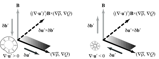
Figure 1: Turbulent electromotive force due to the mis-alignment of the mean magnetic field B from the gradient of mean density or internal energy, $\nabla\overline{\rho}$ or $\nabla Q$. Cases for the local expansion (positive dilatation) (left) and the local contraction (negative dilatation) (right).

Integrating (3) and (4) with respect to time, we get approximate expressions for ${\textbf{u}}^{\prime}$ and ${\textbf{b}}^{\prime}$. Then, the EMF due to turbulent dilatation, $\langle{{\textbf{u}}^{\prime}\times{\textbf{b}}^{\prime}}\rangle_{\textrm{TD}}$, is given as

$$\left\langle{{\textbf{u}}^{\prime}\times{\textbf{b}}^{\prime}}\right\rangle_{\textrm{TD}}\simeq - (\gamma_{\textrm{s}}-1)^{2}\tau_{u}\tau_{b}\tau_{q}\left\langle{(\nabla\cdot{\textbf{u}}^{\prime})^{2}}\right\rangle\frac{Q}{\overline{\rho}}\nabla\overline{\rho}\times{\textbf{B}}$$ (5)

$$- (\gamma_{\textrm{s}}-1)\tau_{u}\tau_{b}\tau_{\rho}\left\langle{(\nabla\cdot{\textbf{u}}^{\prime})^{2}}\right\rangle\nabla Q\times{\textbf{B}},$$

where $\tau_{u}$ and $\tau_{b}$ are the characteristic times of velocity and magnetic-field evolutions, respectively. Equation (5) infers that in the presence of the obliqueness between the mean magnetic field B and the gradient of mean density, $\nabla\overline{\rho}$, and/or the gradient of mean internal energy, $\nabla Q$, the EMF is induced in the direction of ${\textbf{B}}\times\nabla\overline{\rho}$ and/or ${\textbf{B}}\times\nabla Q$, mediated by the turbulent dilatation. It is important to note that the direction of $\langle{{\textbf{u}}^{\prime}\times{\textbf{b}}^{\prime}}\rangle_{\textrm{TD}}$ is always in the direction of ${\textbf{B}}\times\nabla\overline{\rho}$ and/or ${\textbf{B}}\times\nabla Q$, independent of the sign of turbulent dilatation (Fig. 1).

2 Equilibrium state and disturbance

In this work, we study a large-scale instability of compressible MHD turbulence: How do the mean or large-scale fields evolve under the influence of the turbulent transport represented by turbulent correlations such as the turbulent mass flux $\langle{\rho^{\prime}{\textbf{u}}^{\prime}}\rangle$, Reynolds stress $\langle{{\textbf{u}}^{\prime}{\textbf{u}}^{\prime}}\rangle$, turbulent Maxwell stress $\langle{{\textbf{b}}^{\prime}{\textbf{b}}^{\prime}}\rangle$, turbulent internal-energy flux $\langle{q^{\prime}{\textbf{u}}^{\prime}}\rangle$, EMF $\langle{{\textbf{u}}^{\prime}\times{\textbf{b}}^{\prime}}\rangle$, etc. appearing in the mean-field equations. For this purpose, a mean-field quantity $F$ is divided into the equilibrium unperturbed state $F_{0}$ and the deviation from it or disturbance, $\delta F$, as $F=F_{0}+\delta F$ with the disturbance being much smaller than the equilibrium field: $|\delta F|\ll|F_{0}|$.

In this work, for the sake of simplicity, we assume simplified equilibrium mean fields for the velocity and magnetic field in the rectangular coordinate system $(x,y,z)$:

$${\textbf{U}}=\textbf{U}_{0}+\delta{\textbf{U}}=\delta{\textbf{U}}=\left({\delta U^{x},\delta U^{y},\delta U^{z}}\right),$$ (6)

$${\textbf{B}}=\textbf{B}_{0}+\delta{\textbf{B}}=\left({B_{0},0,0}\right)+\left({\delta B^{x},\delta B^{y},\delta B^{z}}\right).$$ (7)

The mean equilibrium velocity ${\textbf{U}}_{0}$ is assumed to be zero (${\textbf{U}}_{0}=0$), and the mean equilibrium magnetic field ${\textbf{B}}_{0}$ is put in the $x$ direction transverse to the mean equilibrium density gradient $\nabla\rho_{0}$ and uniform ($B_{0}={\textrm{const}}.$).

We decompose the mean-field equations into $F_{0}$ and $\delta F$ with (6) and (7), we have equations of disturbances:

$$\frac{\partial\delta\rho}{\partial t}+(\delta{\textbf{U}}\cdot\nabla)\rho_{0}+\rho_{0}\nabla\cdot\delta{\textbf{U}}=-\nabla\cdot\langle{\rho^{\prime}{\textbf{u}}^{\prime}}\rangle_{1},$$ (8)

$$\frac{\partial}{\partial t}\rho_{0}\delta U^{\alpha}=-\frac{\partial\delta P}{\partial x^{\alpha}}+\frac{\partial}{\partial x^{a}}\mu\left({\frac{\partial\delta U^{\alpha}}{\partial x^{a}}+\frac{\partial\delta U^{a}}{\partial x^{\alpha}}}\right)+({\textbf{J}}_{0}\times\delta{\textbf{B}})^{\alpha}+(\delta{\textbf{J}}\times{\textbf{B}}_{0})^{\alpha}$$ (9)

$$-\frac{\partial}{\partial x^{a}}\left[{\delta\rho\left({\langle{u^{\prime}{}^{a}u^{\prime}{}^{\alpha}}\rangle_{0}-\frac{1}{\mu_{0}\rho_{0}}\langle{b^{\prime}{}^{a}b^{\prime}{}^{\alpha}}\rangle_{0}}\right)+\delta U^{a}\langle{\rho^{\prime}u^{\prime}{}^{\alpha}}\rangle_{0}+\delta U^{\alpha}\langle{\rho^{\prime}u^{\prime}{}^{a}}\rangle_{0}}\right],$$

$$\frac{\partial}{\partial t}\left({\rho_{0}\delta Q+\delta\rho Q_{0}}\right)+\nabla\cdot\left({\rho_{0}\delta{\textbf{U}}Q_{0}}\right)$$ (10)

$$=\nabla\cdot\left({\frac{\kappa}{C_{v}}\nabla\delta Q}\right)-\nabla\cdot\left({\delta\overline{\rho}\langle{q^{\prime}{\textbf{u}}^{\prime}}\rangle_{0}+\delta Q\langle{\rho^{\prime}{\textbf{u}}^{\prime}}\rangle_{0}}\right)$$

$$+\delta{\textbf{U}}\langle{\rho^{\prime}q^{\prime}}\rangle_{0}-(\gamma_{s}-1)\left[{\rho_{0}Q_{0}\nabla\cdot\delta{\textbf{U}}+\delta\rho\langle{q^{\prime}\nabla\cdot{\textbf{u}}^{\prime}}\rangle_{0}+\delta Q\langle{\rho^{\prime}\nabla\cdot{\textbf{u}}^{\prime}}\rangle_{0}}\right],$$

$$\frac{\partial{\delta\textbf{B}}}{\partial t}=\nabla\times\left({\delta{\textbf{U}}\times{\textbf{B}}_{0}}\right)+\eta\nabla^{2}\delta{\textbf{B}}+\nabla\times\langle{{\textbf{u}}^{\prime}\times{\textbf{b}}^{\prime}}\rangle_{1}$$ (11)

and the solenoidal condition of the magnetic field: $\nabla\cdot\delta{\textbf{B}}=0$.

The pressure and internal-energy perturbations, $\delta P$ and $\delta Q$, can be expressed in terms of the density perturbation $\delta\rho$ with the speed of sound $c_{\textrm{s}}$ as

$$\delta P=\left({\gamma_{\textrm{s}}-1}\right)\left({\rho_{0}\delta Q+Q_{0}\delta\rho}\right)=c_{\textrm{s}}^{2}\delta\rho.$$ (12)

Then, there is no need to solve the internal-energy equation.

The turbulent correlations in the mean-field perturbation equations are given as

$$\langle{\rho^{\prime}{\textbf{u}}^{\prime}}\rangle_{0}=-\kappa_{\rho}\nabla\rho_{0},\;\;\;\;\;\langle{\rho^{\prime}{\textbf{u}}^{\prime}}\rangle_{1}=-\kappa_{\rho}\nabla\delta\rho,$$ (13)

$$\langle{u^{\prime}{}^{\alpha}u^{\prime}{}^{\beta}}\rangle_{0}-\frac{1}{\mu_{0}\overline{\rho}}\langle{b^{\prime}{}^{\alpha}b^{\prime}{}^{\beta}}\rangle_{0}=-\nu_{\textrm{K}}\left({\frac{\partial U_{0}^{\beta}}{\partial x^{\alpha}}+\frac{\partial U_{0}^{\alpha}}{\partial x^{\beta}}}\right)+\nu_{\textrm{M}}\left({\frac{\partial B_{0}^{\beta}}{\partial x^{\alpha}}+\frac{\partial B_{0}^{\alpha}}{\partial x^{\beta}}}\right)\left/{\mu_{0}\overline{\rho}\rule{0.0pt}{12.91663pt}}\right.=0,$$ (14)

$$\langle{{\textbf{u}}^{\prime}\times{\textbf{b}}^{\prime}}\rangle_{1}=-\eta_{\textrm{T}}\delta{\textbf{J}}+\alpha\delta{\textbf{B}}+\gamma\delta\mbox{\boldmath$\Omega$}+\chi_{\rho}{\textbf{B}}_{0}\times{\nabla\delta\rho}+\chi_{\rho}\delta{\textbf{B}}\times{\nabla\rho_{0}},$$ (15)

where $\kappa_{\rho}$, $\nu_{\textrm{K}}$, and $\nu_{\textrm{M}}$ are the transport coefficients. Note that (14) gives no contribution because of the assumptions (6) and (7).

3 Normal mode analysis of the mean-field equations

We analyse an arbitrary disturbance into a complete set of normal modes, and examine the stability of each of these modes characterised by a wave number $k$. The disturbances are expressed in terms of two-dimensional periodic waves as

$$\delta F=\hat{f}(z)\exp[i(k^{x}x+k^{y}y)-i\omega_{\textbf{k}}t],$$ (16)

where $\delta F=(\delta\rho,\delta{\textbf{U}},\delta Q,\delta{\textbf{B}})$ and $\hat{f}=(\hat{\rho},\hat{\textbf{u}},\hat{q},\hat{\textbf{b}})$. In general this formalism leads to a two-point boundary eigenvalue problem for the functions $\hat{f}(z)$. Here, as the simplest possible case, we assume that the amplitudes of disturbances, $\hat{f}$, do not depend on the vertical coordinate $z$ and constant, which will be relaxed in subsequent papers. Under this assumption, the equations of perturbations are

$$\left({-k^{2}\kappa_{\rho}+i\omega_{\textbf{k}}}\right)\hat{\rho}+ik^{x}\rho_{0}\hat{u}^{x}+ik^{y}\rho_{0}\hat{u}^{y}+\frac{d\rho_{0}}{dz}\hat{u}^{z}=0,$$ (17)

$$-ik^{x}c_{\textrm{s}}^{2}\hat{\rho}+\left({\kappa_{\rho}\frac{d^{2}\rho_{0}}{dz^{2}}+i\omega_{\textbf{k}}\rho_{0}}\right)\hat{u}^{x}=0,$$ (18)

$$-ik^{y}c_{\textrm{s}}^{2}\hat{\rho}+\left({\kappa_{\rho}\frac{d^{2}\rho_{0}}{dz^{2}}+i\omega_{\textbf{k}}\rho_{0}}\right)\hat{u}^{y}-ik^{y}B_{0}\hat{b}^{x}+ik^{x}B_{0}\hat{b}^{y}=0,$$ (19)

$$ik^{x}\kappa_{\rho}\hat{u}^{x}+ik^{y}\kappa_{\rho}\hat{u}^{y}+\left({\kappa_{\rho}\frac{d^{2}\rho_{0}}{dz^{2}}+i\omega_{\textbf{k}}\rho_{0}}\right)\hat{u}^{z}+ik^{x}B_{0}\frac{d\rho_{0}}{dz}\hat{b}^{z}=0,$$ (20)

$$k^{2}\gamma\hat{u}^{x}-ik^{y}B_{0}\hat{u}^{y}+\left({-k^{2}\eta_{\textrm{T}}+\chi_{\rho}\frac{d^{2}\rho_{0}}{dz^{2}}+i\omega_{\textbf{k}}}\right)\hat{b}^{x}+ik^{y}\alpha\hat{b}^{z}=0,$$ (21)

$$\left({k^{2}\gamma+ik^{x}B_{0}}\right)\hat{u}^{y}+\left({-k^{2}\eta_{\textrm{T}}+\chi_{\rho}\frac{d^{2}\rho_{0}}{dz^{2}}+i\omega_{\textbf{k}}}\right)\hat{b}^{y}-ik^{x}\alpha\hat{b}^{z}=0,$$ (22)

$$ik^{x}B_{0}\hat{u}^{x}+k^{2}\gamma\hat{u}^{z}-ik^{y}\alpha\hat{b}^{x}+ik^{x}\alpha\hat{b}^{y}+\left({-k^{2}\eta_{\textrm{T}}+i\omega_{\textbf{k}}}\right)\hat{b}^{z}=0.$$ (23)

This system of equations (17)-(23) with the solenoidal conditions for the magnetic field is analysed. One of the dispersion relations is given by

$$\chi_{\rho}\frac{d^{2}\rho_{0}}{dz^{2}}-\eta_{\textrm{T}}k^{2}+i\omega_{\textbf{k}}=0.$$ (24)

From this, the $\alpha$ component of large-scale magnetic-field disturbance is written as

$$\delta B^{\alpha}=\hat{b}^{\alpha}\exp\left[{\left({-\eta_{\textrm{T}}k^{2}+\chi_{\rho}\frac{d^{2}\rho_{0}}{dz^{2}}}\right)t}\right]\exp[i(k^{x}x+k^{y}y)].$$ (25)

The first term in the temporal evolution part arises from the turbulent magnetic diffusivity $\eta_{\textrm{T}}$. The growth of the mean-field perturbations are suppressed by $\eta_{\textrm{T}}$. This effect is strongest at small scales where the wave number $k$ is large. On the other hand, in the presence of a strong mean density inhomogeneity such that

$$\chi_{\rho}\frac{d^{2}\rho_{0}}{dz^{2}}>\eta_{\textrm{T}}k^{2},$$ (26)

the second or $\chi_{\rho}$-related term in the temporal evolution part contributes to the growth of mean-field perturbations. This large-scale instability, the magnetoclinicity instability, is important only in the region where the density variance is strong enough since it also depends on $\chi_{\rho}(\propto\langle{\rho^{\prime}{}^{2}}\rangle)$.

4 Instability across the strong density variation

In order to quantitatively evaluate the magnetoclinicity effect, we consider a simplest possible spatial profile of the unperturbed density $\rho_{0}(z)$ as

$$\rho_{0}(z)=\rho_{\textrm{m}}-\rho_{\textrm{d}}\tanh\left({{z}/{z_{\textrm{d}}}}\right),$$ (27)

where $\rho_{\textrm{m}}[=(\rho_{>}+\rho_{<})/2]$ is the reference (average) density, $\rho_{\textrm{d}}[=(\rho_{>}-\rho_{<})/2]$ the density difference, and $z_{\textrm{d}}$ the depth of mean density variation. For the spatial distribution of unperturbed density (27), the first and second derivatives are given as

$$\frac{d\rho_{0}(z)}{dz}=-\frac{\rho_{\textrm{d}}}{z_{\textrm{d}}}\frac{1}{\cosh^{2}\left({{z}/{z_{\textrm{d}}}}\right)},\;\;\;\;\;\frac{d^{2}\rho_{0}(z)}{dz^{2}}=+\frac{2\rho_{\textrm{d}}}{z_{\textrm{d}}^{2}}\frac{\tanh(z/z_{\textrm{d}})}{\cosh^{2}\left({{z}/{z_{\textrm{d}}}}\right)}.$$ (28)

The schematic spatial distribution of the unperturbed density, its first and second derivatives, as well as the setup considered, are depicted in Fig. 2.

Figure 2: Schematic spatial distributions of (a) the unperturbed density $\rho_{0}(z)$, (b) its first derivative with respect to $z$, $d^{2}\rho_{0}/dz$, (c) the second derivative $d^{2}\rho_{0}/dz^{2}$, and (d) the setup with transverse B.

With this density configuration, the second derivative is positive in the upper layer (low density region) and negative in the lower layer (high density region) as

$$\frac{d^{2}\rho_{0}}{dz^{2}}\left\{{\begin{array}[]{ll}\rule{0.0pt}{8.61108pt}>0&(z>0,\;\rho_{<}:\;\mbox{low density}),\\ \rule{0.0pt}{8.61108pt}<0&(z<0,\;\rho_{>}:\;\mbox{high density}).\end{array}}\right.$$ (29)

It follows from (25) that the mean magnetic-field disturbance can increase in the low density (positive $z$) side, and decays in the high-density (negative $z$) side. The lower the wave number $k$ is, the larger the growth rate of the perturbed magnetic field is. In this sense, this magnetoclinicity effect is more suitable for producing large-scale magnetic-field structures than small-scale ones. The growth rate also depends on how much large transport coefficient $\chi_{\rho}$ is. The magnitude of $\chi_{\rho}$ reflects the magnitude of density variance $\langle{\rho^{\prime}{}^{2}}\rangle$. If the high $\chi_{\rho}$ region is spatially localised, the instability region of the large magnetic field is also spatially localised. A region with a strong mean density gradient $\nabla\overline{\rho}$ is favourable for high density variance $\langle{\rho^{\prime}{}^{2}}\rangle$, since $\langle{\rho^{\prime}{}^{2}}\rangle$ is generated by strong $\nabla\overline{\rho}$ coupled with $-\langle{\rho^{\prime}{\textbf{u}}^{\prime}}\rangle$. We stress again here that although the arguments here make physical sense, a global analysis involving a two-point boundary value problem is necessary to elucidate the mechanisms.

References

- Yoshizawa (1984) A Yoshizawa (1984) Statistical analysis of the deviation of the Reynolds stress from its eddy-viscosity representation, Phys Fluids 27:1377–1387
- Yokoi (2020) N Yokoi (2020) Turbulence, Transport and Reconnection, in D. MacTaggart and A. Hillier (eds.), Topics in Magnetohydrodynamic Topology, Reconnection and Stability Theory, CISM International Centre for Mechanical Sciences 591, Springer: 177–265
- Yokoi (2018a) N Yokoi (2018a) Electromotive force in strongly compressible magnetohydrodynamic turbulence, J Plasma Phys 84:735840501-1–26
- Yokoi (2018b) N Yokoi (2018b) Mass and internal-energy transports in strongly compressible magnetohydrodynamic turbulence, J Plasma Phys 84:7758140603-1–30
- Yokoi (2013) N Yokoi (2013) Cross helicity and related dynamo, Geophys Astrophys Fluid Dyn 107:114-184