When is the convex hull of a Lévy path smooth?

Abstract.

We characterise, in terms of their transition laws, the class of one-dimensional Lévy processes whose graph has a continuously differentiable (planar) convex hull. We show that this phenomenon is exhibited by a broad class of infinite variation Lévy processes and depends subtly on the behaviour of the Lévy measure at zero. We introduce a class of strongly eroded Lévy processes, whose Dini derivatives vanish at every local minimum of the trajectory for all perturbations with a linear drift, and prove that these are precisely the processes with smooth convex hulls. We study how the smoothness of the convex hull can break and construct examples exhibiting a variety of smooth/non-smooth behaviours. Finally, we conjecture that an infinite variation Lévy process is either strongly eroded or abrupt, a claim implied by Vigon’s point-hitting conjecture. In the finite variation case, we characterise the points of smoothness of the hull in terms of the Lévy measure.

1. Introduction and main results

Convex hulls of stochastic processes, including Brownian motion and Lévy processes, have been the focus of many studies for decades, see e.g. [1, 9, 22, 18, 14, 28] and the references therein. The boundary of the convex hull of the range of a planar Brownian motion consists of piecewise linear segments but is well-known to be smooth (i.e. continuously differentiable) everywhere [14]. The convex hull of a graph of a path of a standard Cauchy process also possesses a smooth boundary almost surely [9], a fact not easily discerned from the simulation in Figure 1.1 below (but cf. discussion following Theorem 1.2 below). Since the law of the graph of the standard Cauchy process scales linearly in time, it is natural to ask whether smoothness of the hull occurs at all for Lévy process without a linear scaling property (note that the range of a planar Brownian motion also possesses a temporal scaling property). In this paper we characterise (in terms of transition laws) what turns out to be a rich and interesting class of Lévy processes whose graphs have smooth convex hulls almost surely. We study its properties by analysing how the smoothness of the hull of a graph may fail for a general Lévy process (see YouTube [4] for a short presentation of our results).

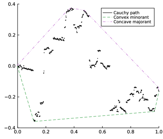
Figure 1.1. The path of a Cauchy process and its convex hull.

The boundary of the convex hull of the graph of a Lévy process $X$ (see [31] for background on Lévy processes) over a finite interval $[0,T]$ is a union of the graphs of the convex minorant and the concave majorant, i.e. the largest convex and smallest concave functions dominating the path pointwise from below and above, respectively (see Figure 1.1). The minorant and majorant are piecewise linear functions for any Lévy process $X$. The set of slopes $\mathcal{S}\subset\mathbb{R}$ of the convex minorant, which has the same law as the set of slopes of the concave majorant (see e.g. [17, Thm 11]), plays a key role in the question of smoothness of the boundary of the hull. Unless otherwise stated, $X$ is not compound Poisson with drift (in this case $\mathcal{S}$ is clearly finite and the smoothness cannot occur), making $X_{t}$ diffuse for all $t>0$ [20, Lem. 15.22] and thus the cardinality of the set of slopes $\mathcal{S}$ infinite [17, Thm 11]. The following zero-one law characterises the local finiteness of $\mathcal{S}$ in terms of the increments of $X$. The characterisation holds for all Lévy processes $X$ with diffuse increments.

Theorem 1.1.

For any measurable set $I\subseteq\mathbb{R}$, the set $\mathcal{S}\cap I$ is either a.s. finite or a.s. infinite. Moreover, the cardinality $|\mathcal{S}\cap I|$ of the intersection $\mathcal{S}\cap I$ is infinite almost surely if and only if

(1.1) $$\int_{0}^{1}\mathds{P}(X_{t}/t\in I)\frac{\mathrm{d}t}{t}=\infty.$$

Theorem 1.1 follows from a novel zero-one law for stick-breaking processes in Theorem 3.1 and Corollary 3.2, established in Section 3 below, and the characterisation of the law of convex minorant of a Lévy process (see e.g. [17]). Since the set of slopes of the concave majorant of the path of $X$ has the law of $\mathcal{S}$, Theorem 1.1 can be used to establish implies the following characterisation of the smoothness of the convex hull.

Theorem 1.2.

The boundary of the convex hull of the graph $t\mapsto(t,X_{t})$, $t\in[0,T]$, of a path of any Lévy process $X$ is continuously differentiable (as a closed curve in $\mathbb{R}^{2}$) a.s. if and only if (1.1) holds for all bounded intervals $I$ in $\mathbb{R}$. Moreover, this is equivalent to the set $\mathcal{S}$ being dense in $\mathbb{R}$ a.s.

It is clear that if the set of slopes $\mathcal{S}$ is not dense in $\mathbb{R}$, the convex hull cannot possess a smooth boundary. Indeed, a gap in $\mathcal{S}$ (i.e. an open interval contained in the complement $\mathbb{R}\setminus\mathcal{S}$) results in the jump of the derivative of the convex minorant and concave majorant (see Section 4.2 below for the proof of Theorem 1.2). Intuitively, as suggested by the simulation in Figure 1.1, $\mathcal{S}$ is dense if every contact point of $X$ with the boundary of the hull is both preceded and followed by infinitely many contact points between the path and the boundary. More generally, Theorem 1.1 (applied to intervals $I=(a,b)$ with rational $a<b$) implies that, interestingly, the set $\mathcal{L}(\mathcal{S})$ of the accumulation points (see Appendix A for definition) of the random set $\mathcal{S}$ is almost surely constant for any Lévy process $X$. Theorem 1.2 thus states that the convex hull of the path of $X$ has a smooth boundary if and only if $\mathcal{L}(\mathcal{S})=\mathbb{R}$ a.s. Note that the criterion in Theorem 1.1 depends neither on the time horizon $T$ nor (by the Lévy-Itô decomposition of $X$) on the behaviour of the Lévy measure of $X$ on the complement of any neighbourhood of zero, even though the set of slopes $\mathcal{S}$ does depend on both.

It was conjectured (without proof) in [3, Rem. 3.4.4] that if the paths of $X$ have infinite variation, then $\mathcal{S}$ has finitely many points on every interval $(a,b)$ if and only if (1.1) fails for all $a<b$. This is implied by Theorem 1.1 above and is furthermore equivalent to $\mathcal{L}(\mathcal{S})=\emptyset$ a.s. Moreover, as we will see below (Proposition 1.3), since $X$ is not compound Poisson with drift, $\mathcal{L}(\mathcal{S})=\emptyset$ a.s. in fact implies that $X$ must be of infinite variation.

An infinite variation process $X$ is abrupt if the following Dini derivatives are infinite at every local minimum $t$ of the path of $X$, $\limsup_{\varepsilon\uparrow 0}(X_{t+\varepsilon}-X_{t-})/\varepsilon=-\infty$ and $\liminf_{\varepsilon\downarrow 0}(X_{t+\varepsilon}-X_{t})/\varepsilon=\infty$, where $X_{t-}$ is the left limit of the trajectory at time $t$. The notion of abruptness, introduced by Vigon in his PhD thesis [36, Def. 12.1.1] (see also [34, Def. 1.1]), captures Lévy processes that approach and leave very rapidly each local minimum of their trajectory. Interestingly, the main result [34, Thm 1.3] states that an infinite variation process $X$ is abrupt if and only if condition (1.1) fails for all intervals in $\mathbb{R}$. Since the minimum is a contact point between the path of $X$ and its convex minorant, abrupt Lévy processes are unlikely to have smooth convex minorants. In fact, the criteria in Theorem 1.2 and [34, Thm 1.3] imply that a Lévy process $X$ is abrupt if and only if $\mathcal{L}(\mathcal{S})=\emptyset$ a.s. An eroded Lévy process $X$ defined in [35, Def. 1.2] (see also [36, App. D, p. 10]) has infinite variation and the following Dini derivatives equal to zero at every local minimum $t$ of the path of $X$, $\limsup_{\varepsilon\uparrow 0}(X_{t+\varepsilon}-X_{t-})/\varepsilon=0$ and $\liminf_{\varepsilon\downarrow 0}(X_{t+\varepsilon}-X_{t})/\varepsilon=0$. These processes approach and leave their local minima very slowly and are good candidates to possess a smooth convex minorant. However, it follows from [35, Thm 1.4] (which can be also be derived from [34, Prop 3.6]) and Theorem 1.1 that an infinite variation Lévy process is eroded if and only if $0\in\mathcal{L}(\mathcal{S})$ a.s. is approached continuously by the slopes of the minorant from both sides, i.e. $0\in\mathcal{L}^{-}(\mathcal{S})\cap\mathcal{L}^{+}(\mathcal{S})$ a.s. (see Appendix A below for the definition of $\mathcal{L}^{\pm}(\mathcal{S})$).

It is clear that, if $X$ is abrupt, then $(X_{t}-rt)_{t\geq 0}$ is also abrupt for any $r\in\mathbb{R}$. However, this invariance may fail for an eroded process. We define a Lévy process $X$ to be strongly eroded if $(X_{t}-rt)_{t\geq 0}$ is eroded for every $r\in\mathbb{R}$, which is equivalent to $\mathcal{L}^{-}(\mathcal{S})\cap\mathcal{L}^{+}(\mathcal{S})=\mathbb{R}$ a.s. Since the interior of $\mathcal{L}(\mathcal{S})$ is contained in $\mathcal{L}^{-}(\mathcal{S})\cap\mathcal{L}^{+}(\mathcal{S})\subseteq\mathcal{L}(\mathcal{S})$ by definition, the process $X$ is strongly eroded if and only if $\mathcal{L}(\mathcal{S})=\mathbb{R}$ a.s. or, equivalently, if the boundary of its convex hull is smooth. Since the respective criteria on the law of $X$ in Theorem 1.2 and [34, Thm 1.3] are not complementary, an interesting question, closely related to Vigon’s point-hitting conjecture discussed below (see Conjecture 1.10), is which (if any) infinite variation processes satisfy (1.1) for some bounded intervals $I$ but not for others. In particular, are there any eroded processes that are not strongly eroded? (See Section 1.1 below for further discussion of these questions.)

The class of strongly eroded Lévy processes, defined in terms of the transition probabilities by the criterion in Theorem 1.2, has a rich structure. For example, it contains families of processes with symmetric and asymmetric Lévy measures, including a standard Cauchy process but excluding all non-standard Cauchy (i.e. weakly 1-stable) processes with asymmetric Lévy measures, see Section 2 below. Moreover, a strongly eroded process has no Gaussian component (by Theorem 1.8(ii-a)) and, since it satisfies $\mathcal{L}(\mathcal{S})=\mathbb{R}$ a.s., has paths of infinite variation (by Proposition 1.3). Its Blumenthal–Getoor index is thus greater or equal to one while the related index $\beta_{-}$, defined in (1.5) below (cf. [29]), is less or equal to one (see Proposition 1.6). More generally, for any strongly eroded Lévy process $X$, the Lévy process $X+Y$ is strongly eroded for any Lévy process $Y$ of finite variation (see Proposition 1.5 below). In contrast, if $Y$ and $X$ are both strongly eroded and independent of each other, the Lévy process $X+Y$ need not (but, of course, could) be strongly eroded, see Example 2.6 below. The properties of strongly eroded Lévy processes will be discussed in more detail in the remainder of Section 1 and in Section 2.

It is natural to attempt to construct the non-random set of limit slopes $\mathcal{L}(\mathcal{S})$ directly from the characteristics of an arbitrary Lévy process $X$. It turns out that, if $X$ is of finite variation, $\mathcal{L}(\mathcal{S})$ is a singleton given by the natural drift of the process, see Table 1 below for an overview of our results. In the infinite variation case, we characterise $\mathcal{L}(\mathcal{S})$ up to Conjecture 1.9 stated below, which is implied by Vigon’s point-hitting conjecture [35, Conj. 1.6] (see the discussion of Conjectures 1.9 and 1.10 below). More precisely, if Vigon’s conjecture were true, our sufficient condition for $X$ to be strongly eroded (i.e. $\mathcal{L}(\mathcal{S})=\mathbb{R}$ a.s.), given in terms of the characteristic exponent of $X$, would also be necessary, and its complement would imply abruptness (i.e. $\mathcal{L}(\mathcal{S})=\emptyset$ a.s.). Moreover, via Orey’s process in Example 2.7 below, if Conjecture 1.10 were true, there would exist a strongly eroded Lévy processes whose path variation is arbitrarily close to two. This is in contrast to all known examples of strongly eroded Lévy processes, which turn out to have Blumenthal–Getoor index equal to one (see Section 2 below). However, if Vigon’s conjecture is not true, there would exist an infinite variation Lévy process with slopes of the convex minorant accumulating at some deterministic values but not at others. Differently put, in this case the non-random set $\mathcal{L}(\mathcal{S})$ would be a proper closed subset of $\mathbb{R}$, implying that kinks in the boundary of the hull would constitute a proper subset of the contact points between the boundary and the closure (in $\mathbb{R}^{2}$) of the graph of the path. As it is not easy to imagine a boundary of the hull of the path being smooth in some regions but not in others, our results could perhaps be viewed as further evidence for Vigon’s point-hitting conjecture.

1.1. Where and how does the continuous differentiability of the boundary fail?

This change of perspective sheds light on where the smoothness features of the boundary discussed above come from. Before stating our results in detail, we give an overview in Table 1. Let $C:[0,T]\to\mathbb{R}$ denote the piecewise linear convex minorant of the path of $X$ on $[0,T]$, see e.g. [17, Thm 11]. Its right-derivative $C^{\prime}:(0,T)\to\mathbb{R}$ is a non-decreasing piecewise constant function with image $\{C^{\prime}(x)|0<x<T\}\supset\mathcal{S}$. Differently put, for every $r\in\mathcal{S}$ there exists a maximal open interval $I_{r}\subset(0,T)$, satisfying $C^{\prime}(I_{r})=\{r\}$. Note that, in general, $C^{\prime}$ may but need not be discontinuous at a boundary point of $I_{r}$. However, as an increasing right-continuous process, its path is completely determined by the set $\mathcal{S}$ of values on the dense set $\bigcup_{r\in\mathcal{S}}I_{r}$ and its discontinuities are in a one-to-one relationship with the gaps of $\mathcal{S}$.

The second derivative (as a distribution) is given by a positive Radon measure $\mathrm{d}C^{\prime}$ on $(0,T)$. Since the set of slopes of the concave majorant and the convex minorant have the same law, the second derivative of the concave majorant has the same law as the (negative) Radon measure $-\mathrm{d}C^{\prime}$. Thus, the derivative of the boundary of the convex hull over the open interval $(0,T)$ is discontinuous at a point if and only if the point is an atom of the measure $\mathrm{d}C^{\prime}$. Over the set $\{0,T\}\subset[0,T]$, the discontinuity of the boundary occurs if and only if the derivative $C^{\prime}$ is either bounded below or above.

Lévy process $X$	Derivative $C^{\prime}$ and the limt set $\mathcal{L}(\mathcal{S})$	Measure $\mathrm{d}C^{\prime}$
Finite variation	$C^{\prime}$ bounded below and above; $C^{\prime}$ discontinuous on boundary $\partial I_{r}$, $\forall r\in\mathcal{S}$; $\mathcal{L}(\mathcal{S})=\{\gamma_{0}\}$, where $\gamma_{0}=\lim_{t\downarrow 0}X_{t}/t$ a.s., and $\gamma_{0}\notin\mathcal{S}$	atomic; atoms accumulate from left/right or from both sides at a unique (random) accumulation point in $[0,T]$
Infinite variation & $\mathfrak{s}_{1}$ locally integrable	$C^{\prime}$ discontinuous on boundary $\partial I_{r}$, $\forall r\in\mathcal{S}$; $-\lim_{t\downarrow 0}C^{\prime}(t)=\lim_{t\uparrow T}C^{\prime}(t)=\infty$; $\mathcal{L}(\mathcal{S})=\emptyset$	atomic; atoms accumulate only at $0$ and $T$
Infinite variation & $\mathfrak{s}_{1}(r)=\infty$, $\forall r\in\mathbb{R}$	$C^{\prime}$ is continuous on $(0,T)$; $-\lim_{t\downarrow 0}C^{\prime}(t)=\lim_{t\uparrow T}C^{\prime}(t)=\infty$; $\mathcal{L}(\mathcal{S})=\mathbb{R}$	singular continuous

Table 1. Summary of the regularity results of the convex minorant $C:[0,T]\to\mathbb{R}$ of any Lévy process $X$ of infinite activity (i.e. not compound Poisson with drift) over time horizon $T$. The function $\mathfrak{s}_{1}$, defined in (1.2) in terms of the generating triplet of $X$, is either locally integrable or everywhere infinite under Conjecture 1.10. By Theorem 1.8 below, this conjecture is known to hold for most Lévy processes.

Let $\psi$ be the Lévy-Khintchine exponent [31, Def. 8.2] of the Lévy process $X$. Note that $\Re\psi(u)\leq 0$ implies $\Re(1/(1+iur-\psi(u)))>0$ for all $r,u\in\mathbb{R}$, where $\Re z$ is the real part of a complex $z\in\mathbb{C}$ and $i^{2}=-1$. Hence $0<\mathfrak{s}_{1}(r)\leq\infty$ for any $r\in\mathbb{R}$, where

(1.2) $$\mathfrak{s}_{1}(r)\coloneqq\frac{1}{2\pi}\int_{\mathbb{R}}\Re\frac{1}{1+iur-\psi(u)}\mathrm{d}u,\qquad r\in\mathbb{R}.$$

The identity in Theorem B.2 below (first established in [35] for Lévy processes with bounded jumps) yields the following equivalence for any real $a<b$:

(1.3) $$\int_{a}^{b}\mathfrak{s}_{1}(r)\mathrm{d}r<\infty\qquad\text{if and only if}\qquad\int_{0}^{1}\mathds{P}(X_{t}/t\in(a,b))\frac{\mathrm{d}t}{t}<\infty.$$

By definition, $\mathfrak{s}_{1}\in L^{1}_{\mathrm{loc}}(r)$ if and only if $\mathfrak{s}_{1}$ is Lebesgue integrable on a neighbourhood of $r\in\mathbb{R}$. Thus $r\in\mathcal{L}(\mathcal{S})$ is (by (1.3) and Theorem 1.1) equivalent to the condition $\mathfrak{s}_{1}\notin L^{1}_{\mathrm{loc}}(r)$, involving only the characteristic exponent of $X$ and not the law of the increment of $X$. For example, the presence of a non-trivial Brownian component implies that $\mathcal{L}(\mathcal{S})=\emptyset$ and, equivalently, that $\mathcal{S}$ is locally finite a.s.

The sum of the lengths of the open maximal intervals $\{I_{s}:s\in\mathcal{S}\}$ of constancy of $C^{\prime}$ equals the time horizon $T$. As suggested by Table 1, the random Radon measure $\mathrm{d}C^{\prime}$, supported on the complement of $\bigcup_{s\in\mathcal{S}}I_{s}$, must therefore be singular a.s. with respect to the Lebesgue measure. Thus the Lebesgue decomposition of $\mathrm{d}C^{\prime}$ is in general a sum of an atomic and a purely singular continuous components. Moreover, if Conjecture 1.10 holds, only one of these summands is non-trivial for any Lévy process.

The convex minorant of a compound Poisson process with drift has only finitely many faces, making its derivative necessarily discontinuous at all boundary points of its maximal intervals of constancy. If $X$ has infinite activity but finite variation, then $C^{\prime}$ is bounded on $[0,T]$ and discontinuous at every point in $\bigcup_{s\in\mathcal{S}}\partial I_{s}$, but is possibly continuous at the single (random) accumulation point of this set (see Proposition 1.3 below and discussion thereafter for details). If $X$ has too much jump activity or a Brownian component, then $C^{\prime}$ is discontinuous at every point in $\bigcup_{s\in\mathcal{S}}\partial I_{s}$ and infinite on $\{0,T\}$ (see Proposition 1.6 below and the discussion thereafter for details). Hence, for $C$ to be continuously differentiable on the open interval $(0,T)$ (i.e., for $X$ to be strongly eroded), the process $X$ must have sufficient jump activity to be of infinite variation, but not too much, as its index $\beta_{-}$ (1.5) must be bounded above by one. These features are discussed in more detail in the following subsections (see Table 2 in Appendix A for all possible behaviours of the right-derivative of a piecewise linear convex function).

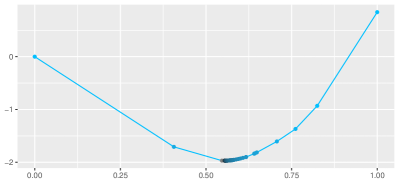
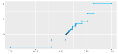
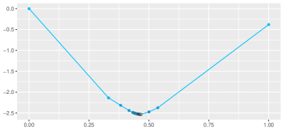
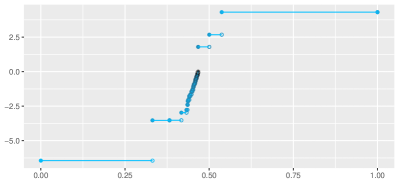
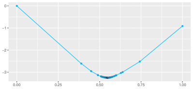
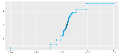
Figure 1.2. Behaviour of $C$ and $C^{\prime}$ for a finite variation infinite activity process $X$. The left panels graph the piecewise linear convex function $C$ (circles mark contact points with the path of $X$). The panels on the right graph the corresponding right-continuous derivative $C^{\prime}$ (jump-size equals the difference of consecutive slopes). The top (resp. middle) panels correspond to right-accumulation (resp. left-accumulation) in Prop. 1.3(b) (resp. Prop. 1.3(c)). Note that in both of these cases, $C^{\prime}$ is only right-continuous at the accumulation point of jump-times. The bottom panels depict two-sided accumulation in Prop. 1.3(a), making $C^{\prime}$ continuous at the unique accumulation point of the jump-times.

1.1.1. Finite variation

Throughout this subsection we assume $X$ has finite variation but infinite activity. Let $\gamma_{0}$ denote the natural drift of $X$ defined in terms of the characteristics in (4.1) below. Since, by Doeblin’s lemma [20, Lem. 15.22], it follows that $\mathds{P}(X_{t}=\gamma_{0}t)=0$ for all $t>0$, the integrals

(1.4) $$I_{-}\coloneqq\int_{0}^{1}\mathds{P}(X_{t}<t\gamma_{0})\frac{\mathrm{d}t}{t}\qquad\text{and}\qquad I_{+}\coloneqq\int_{0}^{1}\mathds{P}(X_{t}>t\gamma_{0})\frac{\mathrm{d}t}{t}$$

satisfy $I_{-}+I_{+}=\infty$, implying that at least one is infinite. Moreover, the integrals $I_{\pm}$ are given in terms of the law of a pure-jump Lévy process $(X_{t}-\gamma_{0}t)_{t\geq 0}$, uniquely determined by the Lévy measure of $X$. Let $\mathcal{L}^{+}(\mathcal{S})$ (resp. $\mathcal{L}^{-}(\mathcal{S})$) be the set of right-accumulation (see Appendix A for definition). Equivalence (1.3) and Theorem 1.1 imply that $s\in\mathcal{L}^{+}(\mathcal{S})$ (resp. $s\in\mathcal{L}^{-}(\mathcal{S})$) if and only if $\mathfrak{s}_{1}\notin L^{1}_{\mathrm{loc}}(s+)$ (resp. $\mathfrak{s}_{1}\notin L^{1}_{\mathrm{loc}}(s-)$), where a function $f$ is in $L^{1}_{\mathrm{loc}}(s+)$ (resp. $L^{1}_{\mathrm{loc}}(s-)$) if and only if $f\cdot\mathds{1}_{(s,\infty)}\in L^{1}_{\mathrm{loc}}(s)$ (resp. $f\cdot\mathds{1}_{(-\infty,s)}\in L^{1}_{\mathrm{loc}}(s)$). In particular, like $\mathcal{L}(\mathcal{S})$, the limit sets $\mathcal{L}^{+}(\mathcal{S})$ and $\mathcal{L}^{-}(\mathcal{S})$ are also constant a.s.

Proposition 1.3.

Let $X$ have infinite activity and finite variation. Then the derivative $C^{\prime}$ (and thus the set of slopes $\mathcal{S}$) is bounded from below and above. $C^{\prime}$ is discontinuous on $\bigcup_{r\in\mathcal{S}}\partial I_{r}$, where $I_{r}$ is the maximal interval of constancy of $C^{\prime}$ corresponding to slope $r$, and the limit set of slopes is a singleton $\mathcal{L}(\mathcal{S})=\{\gamma_{0}\}$ (the natural drift $\gamma_{0}$ of $X$ is defined in (4.1)). Time $v\in[0,T]$ at which the process $(X_{t}-\gamma_{0}t)_{t\geq 0}$ attains its minimum in $[0,T]$ is a.s. unique. If $v>0$, denote the left limit of $C^{\prime}$ at $v$ by $C^{\prime}(v-):=\lim_{t\uparrow v}C^{\prime}(t)$. Then we have:

• if $I_{+}=I_{-}=\infty$, then $v\in(0,T)$, $\mathcal{L}^{-}(\mathcal{S})=\mathcal{L}^{+}(\mathcal{S})=\{\gamma_{0}\}$ and $C^{\prime}(v-)=C^{\prime}(v)=\gamma_{0}$ a.s.;

• if $I_{-}<\infty$, then $v\in[0,T)$ with $\mathds{P}(v=0)>0$, $\mathcal{L}^{-}(\mathcal{S})=\emptyset$, $\mathcal{L}^{+}(\mathcal{S})=\{\gamma_{0}\}$, $C^{\prime}(v)=\gamma_{0}$ a.s. and, on the event $\{v>0\}$, we have $C^{\prime}(v-)<\gamma_{0}$ a.s.;

• if $I_{+}<\infty$, then $v\in(0,T]$ with $\mathds{P}(v=T)>0$, $\mathcal{L}^{+}(\mathcal{S})=\emptyset$, $\mathcal{L}^{-}(\mathcal{S})=\{\gamma_{0}\}$, $C^{\prime}(v-)=\gamma_{0}$ a.s. and, on the event $\{v<T\}$, we have $C^{\prime}(v)>\gamma_{0}$ a.s.

By Rogozin’s criterion (see e.g. [17, Thm 6]), the integral conditions in Proposition 1.3(a) are equivalent to $0$ being regular for both half-lines for the process $(X_{t}-\gamma_{0}t)_{t\geq 0}$. In particular, for the two conditions to hold concurrently it is necessary (but not sufficient) for $X$ to exhibit infinitely many positive and negative jumps in any finite time interval [31, Thm 47.5] and sufficient (but not necessary) for $X$ to be spectrally symmetric. The other cases are also possible since $I_{-}<\infty$ (resp. $I_{+}<\infty$) if $X$ is the difference of two stable subordinators and the positive (resp. negative) jumps have a larger stability index. The following corollary is a simple consequence of Proposition 1.3, equivalence (1.3) and [7, Thm 1]. It characterises which case in Proposition 1.3 occurs in terms of either the Lévy measure $\nu$ or the characteristic exponent $\psi$ (via $\mathfrak{s}_{1}$ defined in (1.2)) of the process $X$.

Corollary 1.4.

Let $X$ have infinite activity but finite variation with natural drift $\gamma_{0}$. Then

$$I_{\pm}=\infty\enskip\iff\enskip\mathfrak{s}_{1}\notin L^{1}_{\mathrm{loc}}(\gamma_{0}\pm)\enskip\iff\enskip\int_{(-1,1)}\frac{\max\{\pm x,0\}}{\int_{0}^{\max\{\pm x,0\}}\overline{\nu}_{\mp}(y)\mathrm{d}y}\nu(\mathrm{d}x)=\infty,$$

where we define $\overline{\nu}_{+}(x):=\nu((x,\infty))$ and $\overline{\nu}_{-}(x):=\nu((-\infty,-x))$ for $x>0$ and $\mp:=-(\pm)$.

Proposition 1.3 and Corollary 1.4 give a complete description (in terms of the characteristics of any infinite activity, finite variation Lévy process $X$) of how the continuity of the derivative $C^{\prime}$ fails, see Figure 1.2 for all possible behaviours. The proof of Proposition 1.3 is based on the criterion in Theorem 1.1 and the crucial fact that, as $t\to 0$, the quotient $X_{t}/t$ a.s. stops visiting closed intervals that do not contain the natural drift $\gamma_{0}$ (since $\lim_{t\to 0}X_{t}/t=\gamma_{0}$ a.s.), see Section 4.1 below for details. The smoothness of the minorant in the infinite variation case is more intricate precisely because in that case we do not have a good understanding in general of how frequently the quotient $X_{t}/t$ visits intervals in $\mathbb{R}$ as $t\to 0$.

1.1.2. Infinite variation

The set of slopes $\mathcal{S}$ is unbounded on both sides for any $X$ of infinite variation, i.e. $\sup\mathcal{S}=-\inf\mathcal{S}=\infty$, and hence $-\lim_{t\downarrow 0}C^{\prime}(t)=\lim_{t\uparrow T}C^{\prime}(t)=\infty$ a.s. (cf. Figure 1.3). Indeed, by Rogozin’s theorem [31, Thm 47.1], asserting that $X_{t}/t$ takes arbitrarily large positive and negative values at arbitrarily small times $t$ for any $X$ of infinite variation, it is impossible for the convex minorant to start at $0$ or end at $T$ with a finite slope: $-\infty=\liminf_{t\downarrow 0}X_{t}/t\geq\inf\mathcal{S}$, and, by time reversal, $\infty=\limsup_{t\downarrow 0}(X_{T}-X_{T-t})/t\leq\sup\mathcal{S}$. Thus the boundary of the convex hull of the path of $X$ is differentiable over the set $\{0,T\}$. Its smoothness over the open interval $(0,T)$, however, is a much more delicate matter. We now state some results to elucidate this structure.

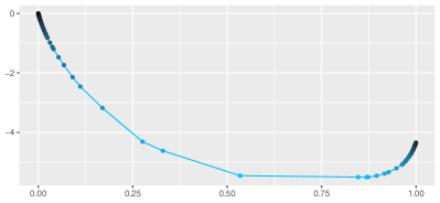
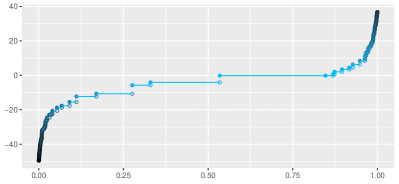
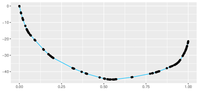
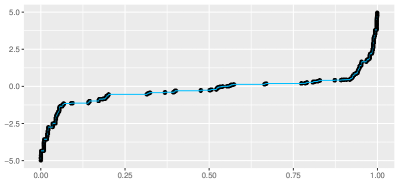
Figure 1.3. The left pictures show the graph of a piecewise linear convex function $C$ with circle marks on $\bigcup_{r\in\mathcal{S}}\partial I_{r}$. The right pictures show the graph of the derivative $C^{\prime}$ with visible points of increase marked with a circle. In the top two pictures, there are no points of continuity as $C^{\prime}$ tends to $\pm\infty$ near times $0$ and $1$. In the bottom two pictures, the function $C$ is continuously differentiable with a singular continuous derivative $C^{\prime}$.

Strongly eroded Lévy process, perturbed by a finite variation process, is still strongly eroded. In fact, for any Lévy process, such a perturbation shifts the set $\mathcal{L}(\mathcal{S})$ by the natural drift, defined in (4.1), of the finite variation process (given a set $A\subset\mathbb{R}$, define $A+b:=\{a+b\,:\,a\in A\}$ for any $b\in\mathbb{R}$ with convention $\emptyset+b:=\emptyset$).

Proposition 1.5.

Suppose the Lévy process $X$ is of the form $X=Y+Z$ for (possibly dependent) Lévy processes $Y$ and $Z$. Let $\mathcal{S}_{X}$ and $\mathcal{S}_{Z}$ be the sets of slopes of the faces of the convex minorants of $X$ and $Z$, respectively. If $Y$ is of finite variation (possibly finite activity) with natural drift $b$ defined in (4.1), then $\mathcal{L}(\mathcal{S}_{X})=\mathcal{L}(\mathcal{S}_{Z})+b$.

The proof of Proposition 1.5 relies on the a.s. limit $b=\lim_{t\downarrow 0}Y_{t}/t$ and the stick-breaking representation of the convex minorant in [17]. The main idea is that if $Z_{t}/t$ frequently visits any neighborhood of a point $x\in\mathbb{R}$ as $t\downarrow 0$, then $X_{t}/t$ visits the neighborhoods of $x+b$ just as frequently. Crucially, when the visits of $Z_{t}/t$ to the neighborhoods of $x$ occur, $Y_{t}/t$ must necessarily be close to $b$ (since the limit $Y_{t_{n}}/t_{n}\to b$ holds along any random sequence of times $t_{n}\downarrow 0$).

Proposition 1.5 and its proof may suggest that, if $Y_{t}/t$ and $Z_{t}/t$ were to visit all open intervals as $t\downarrow 0$ with such frequency that their respective sets of slopes $\mathcal{S}_{Y}$ and $\mathcal{S}_{Z}$ are dense, then the same should be true for $X_{t}/t$. This intuition, however, turns out to be false, as Example 2.6 below illustrates. Intuitively, the reason for this is that the frequent visits of $Y_{t}/t$ and $Z_{t}/t$ to such neighborhoods may be sufficiently rare so that they do not occur simultaneously with sufficient frequency even when $Y$ and $Z$ are independent.

Too much jump activity breaks smoothness. Let $\sigma\geq 0$ be the volatility of the Brownian component of $X$ and define the function $\overline{\sigma}^{2}(u)\coloneqq\int_{(-u,u)}x^{2}\nu(\mathrm{d}x)$ for $u>0$. The lower-activity index $\beta_{-}$ (inspired by Pruitt [29]) and the Blumenthal–Getoor index $\beta_{+}$ (introduced in [12]) are given by

(1.5) $$\beta_{-}\coloneqq\inf\Big{\{}p>0:\liminf_{u\downarrow 0}u^{p-2}\overline{\sigma}^{2}(u)=0\Big{\}}\quad\text{and}\quad\beta_{+}\coloneqq\inf\left\{p>0\,:\,\int_{(-1,1)}|x|^{p}\nu(\mathrm{d}x)<\infty\right\},$$

respectively. It is easy to see that the inequalities $0\leq\beta_{-}\leq\beta_{+}\leq 2$ hold. Since $\beta_{-}$ (resp. $\beta_{+}$) presents a lower (resp. upper) bound on the activity of the Lévy measure $\nu$ at zero, in general we may have $\beta_{-}<\beta_{+}$. However, both indices agree if the tails of $\nu$ are regularly varying at $0$ (e.g. if $X_{t}$ is in the domain of attraction of an $\alpha$-stable law as $t\downarrow 0$).

Proposition 1.6.

If $\int_{1}^{\infty}(1+u^{2}(\sigma^{2}+\overline{\sigma}^{2}(1/u)))^{-1}\mathrm{d}u<\infty$, then $\mathcal{L}(\mathcal{S})=\emptyset$ a.s. and hence $X$ is abrupt. In particular, this is the case if $\sigma^{2}>0$ or $\beta_{-}>1$.

Proposition 1.6 shows that a strongly eroded process necessarily satisfies $\beta_{-}\leq 1\leq\beta_{+}$. This is natural since, in some sense, the running supremum of the process $X$ fluctuates between the functions $t\mapsto t^{1/\beta_{+}}$ and $t\mapsto t^{1/\beta_{-}}$ as $t\downarrow 0$ [31, Prop. 47.24] and the visits of $X_{t}/t$ to compact intervals determine whether $X$ is strongly eroded. In other words, it is natural that strongly eroded processes require the linear map $t\mapsto t$ to lie between the functions $t\mapsto t^{1/\beta_{+}}$ and $t\mapsto t^{1/\beta_{-}}$ as $t\downarrow 0$, which is equivalent to $\beta_{-}\leq 1\leq\beta_{+}$. We remark that, despite the necessary condition on the indices $\beta_{-}$ and $\beta_{+}$ allowing a strict inequality, all our examples of strongly eroded processes lie in the boundary case $\beta_{-}=1=\beta_{+}$. However, as explained in Example 2.7 below, Conjecture 1.10 implies that a strict inequality is feasible for certain strongly eroded Lévy processes.

Too much asymmetry breaks smoothness. Recall that a process creeps upwards (resp. downwards) if $\mathds{P}(T_{(x,\infty)}<\infty,X_{T_{(x,\infty)}}=x)>0$ (resp. $\mathds{P}(T_{(-\infty,x)}<\infty,X_{T_{(-\infty,x)}}=x)>0$) for some $x>0$ (resp. $x<0$), where $T_{A}\coloneqq\inf\{t>0:X_{t}\in A\}$ denotes the first hitting time of set $A\subset\mathbb{R}$ (with convention $\inf\emptyset=\infty$), i.e., if the process crosses levels continuously with positive probability. Processes that creep (upward or downward), all of which are abrupt by [34, Ex. 1.5], tend to have Lévy measures that are asymmetric on a neighborhood of $0$ (see [37] for a characterisation of such processes in terms of $\nu$). For instance, if $\sigma=0$ and $\nu$ is of infinite variation but $\int_{(0,1)}x\nu(\mathrm{d}x)<\infty$ (resp. $\int_{(-1,0)}|x|\nu(\mathrm{d}x)<\infty$), then $X$ creeps upwards (resp. downwards), see [24, Eq. (1.7)] and the subsequent discussion.

These facts suggest that asymmetry tends to produce abrupt processes. This heuristic is also suggested by the inequality $\Re(1/(1+iur-\psi(u)))\leq 1/(1-\Re\psi(u))$, where we note that the characteristic exponent of the symmetrisation $\widehat{X}$ of $X$ (a process with the same law as $X-Y$, where $Y$ is independent of $X$ but shares its law) equals $2\Re\psi$. In particular, under Vigon’s point-hitting conjecture (see Conjecture 1.10 below), (1.3) gives the following implications: (I) if $\widehat{X}$ is abrupt then $X$ is abrupt and (II) if $X$ is strongly eroded then $\widehat{X}$ is strongly eroded. We complement these observations with the following result, further supporting this heuristic.

Proposition 1.7.

Let $X$ be an infinite variation Lévy process and suppose there exist constants $c>1$ and $x_{0}\in(0,\infty]$ such that $\nu([x,y))\geq c\nu((-y,-x])$ for all $0<x<y<x_{0}$. Then $X$ is abrupt.

We stress that the process in Proposition 1.7 is abrupt but need not creep. The assumption in Proposition 1.7 requires, on a neighborhood of $0$, the restriction of $\nu$ on the negative half-line to be absolutely continuous with respect to its restriction on the positive half-line with Radon–Nikodym derivative $\varphi(x)=\nu(\mathrm{d}(-x))/\nu(\mathrm{d}x)$ bounded above by $1/c<1$ (equivalently, $\limsup_{x\downarrow 0}\varphi(x)<1$). This condition is nearly optimal, since there exist strongly eroded processes with positive asymmetry $1-\varphi(x)$ that vanishes (arbitrarily) slowly $1-\varphi(x)\downarrow 0$ as $x\downarrow 0$, see Example 2.10 below. Note that, by using Propositions 1.7 and 1.5 jointly, we obtain a simple recipe to construct abrupt processes with $\beta_{-}\leq 1\leq\beta_{+}$.

Sufficient conditions for $X$ to be strongly eroded (or abrupt). The following theorem, implied by Theorem 1.1 above and the results in [34], shows that most Lévy processes of infinite variation are either strongly eroded or abrupt. Moreover, Theorem 1.8 offers simple conditions to ascertain whether $X$ is strongly eroded or abrupt. The criteria are (mostly) in terms of the behaviour at infinity of the Lévy–Khintchine exponent $\psi$ of $X$. More precisely, it is connected to the ratio $\psi(u)/u$ for large $|u|$. This ratio appears naturally since the characteristic exponent of $X_{t}/t$ is given by $u\mapsto t\psi(u/t)$, whose behaviour for small $t$ is described by the behaviour of $\psi(u)/u$ for large $|u|$.

Let $\Im z$ and $|z|$ denote the imaginary part and the modulus of the complex number $z\in\mathbb{C}$. Recall that $\Re\psi$ (resp. $\Im\psi$) is an even (resp. odd) function on $\mathbb{R}$.

Theorem 1.8.

Let $X$ be a Lévy process of infinite variation with $e^{\psi(u)}=\mathds{E}e^{iuX_{1}}$, $u\in\mathbb{R}$.

• If $\limsup_{u\to\infty}|\psi(u)/u|<\infty$, then $X$ is strongly eroded.

• If $\lim_{u\to\infty}|\psi(u)/u|=\infty$, then $X$ is either abrupt or strongly eroded.

  • If $\lim_{|u|\to\infty}|\Re\psi(u)/u|=\infty$, then $X$ is strongly eroded if and only if $\int_{1}^{\infty}\Re(1/(1-\psi(u)))\mathrm{d}u=\infty$,

  • If the upper and lower limits of $|\Re\psi(u)/u|$ lie in $(0,\infty)$ and $\lim_{|u|\to\infty}|\Im\psi(u)/u|=\infty$, then $X$ is strongly eroded if and only if $\int_{1}^{\infty}u(1+|\Im\psi(u)|^{2})^{-1}\mathrm{d}u=\infty$,

  • If $\lim_{|u|\to\infty}|\Re\psi(u)/u|=0$ and $\lim_{|u|\to\infty}|\Im\psi(u)/u|=\infty$, then $X$ is strongly eroded if and only if we have $\int_{1}^{\infty}(1-\Re\psi(u))(1+|\Im\psi(u)|^{2})^{-1}\mathrm{d}u=\infty$.

In fact, the proof of Theorem 1.8 shows that, under the assumptions of Theorem 1.8, $\mathfrak{s}_{1}$ is either locally bounded (making $X$ strongly eroded) or everywhere infinite (making $X$ abrupt). Cases (i) and (ii) in Theorem 1.8 are in some sense generic, but they do not exhaust the class of infinite variation Lévy processes, see Examples 2.5 and 2.7 below. In fact, Example 2.5 defines a strongly eroded Lévy process, outside of the scope of Theorem 1.8, with the characteristic exponent that fluctuates between linear and superlinear behaviour as $u\to\infty$. However, the class of processes in the union of case (i) and (ii) is closed under addition of independent summands. Similarly, cases (ii-a), (ii-b) and (ii-c) are not exhaustive within (ii). However, for neither case (i) nor case (ii) to hold, it is necessary that $|\psi(u)|$ fluctuate between linear (or sublinear) and superlinear functions of $|u|$. The fact that $X$ has infinite variation if and only if $\int_{1}^{\infty}u^{-2}|\Re\psi(u)|\mathrm{d}u=\infty$ (by Lemma B.5, see also [36, Prop. 1.5.3]) shows that most processes indeed fall within either case (i) or (ii).

A conjectural dichotomy. Our results may be viewed as further evidence for Vigon’s point-hitting conjecture (see Conjecture 1.10 below), whose origins go back to Vigon’s PhD thesis [36, p. 10] in 2002, which implies the following dichotomy for infinite variation Lévy processes:

Conjecture 1.9.

Any infinite variation Lévy process is either abrupt or strongly eroded.

In order to understand the relationship between Conjecture 1.9 and Vigon’s point-hitting conjecture, recall first that the process $X$ hits points if for some $x\in\mathbb{R}$, the hitting time $T_{x}\coloneqq\inf\{t>0:X_{t}=x\}$ is finite with positive probability. If $X$ has infinite variation, [13, Thm 8] (see also [21, Thm 1]) implies that $\mathds{P}(T_{x}<\infty)>0$ for some $x\in\mathbb{R}$ if and only if $\mathds{P}(T_{x}<\infty)>0$ for all $x\in\mathbb{R}$.

Conjecture 1.10 ([35, Conject. 1.6]).

Let $X$ be an infinite variation process and for any $r\in\mathbb{R}$ define the Lévy process $X^{(r)}=(X_{t}-rt)_{t\geq 0}$. Then the following statements are equivalent.

• There exists some $r\in\mathbb{R}$ such that the process $X^{(r)}$ hits points.

• For all $r\in\mathbb{R}$ the process $X^{(r)}$ hits points.

• The process $X$ is abrupt.

By [13, Thm 7] (see also [21, Thm 2]), $\mathfrak{s}_{1}(r)<\infty$ is equivalent to $X^{(r)}$ hitting points (recall the definition of $\mathfrak{s}_{1}$ in (1.2)). Moreover, by the equivalence in (1.3) and [34, Thm 1.3], $X$ is abrupt if and only if $\mathfrak{s}_{1}$ is locally integrable on $\mathbb{R}$. Conjecture 1.10 thus says that the following three statements are equivalent for any infinite variation Lévy process $X$: (i) $\mathfrak{s}_{1}(r)<\infty$ for some $r\in\mathbb{R}$, (ii) $\mathfrak{s}_{1}(r)<\infty$ for all $r\in\mathbb{R}$ and (iii) the function $\mathfrak{s}_{1}$ is locally integrable on $\mathbb{R}$. In particular, under Conjecture 1.10, the function $\mathfrak{s}_{1}$ is either everywhere infinite or locally integrable, thus implying Conjecture 1.9 by Theorem 1.1, equivalence (1.3) and [34, Thm 1.3].

The finiteness of $\mathfrak{s}_{1}(r)$, hinging entirely on the integrability at infinity of the positive bounded function $u\mapsto\Re(1/(1+iur-\psi(u)))$, becomes a focal point under Conjecture 1.10. For instance, Conjecture 1.10 holds if $X$ satisfies the assumptions of either Proposition 1.7 or Theorem 1.8 (the below proofs of these results establish that $\mathfrak{s}_{1}$ is locally finite on $\mathbb{R}$). The condition $\mathfrak{s}_{1}(0)<\infty$ is equivalent to a number of probabilistic statements about the infinite variation process $X$:

• the potential measure of $X$ is absolutely continuous with a bounded density (by [31, Thm 43.3]),

• the point $0$ is regular for itself for the process $X$, i.e. $\mathds{P}(T_{0}=0)=1$ (by [13, Thms 7 & 8]),

• the process $X$ possesses a local time field (by [6, Thm V.1]).

In principle, any of these properties may hold for $X$ but not for some $X^{(r)}$. Conjecture 1.10, which asserts that this is not the case, can thus be equivalently stated by substituting “hitting of points” with any of the three properties in the bullet-point list.

The structure of Conjecture 1.10, in terms of varying drifts, is natural as a number of properties of infinite variation processes are known to be invariant under addition of a deterministic drift and, more generally, under a perturbation by an independent finite variation process $Y$. For instance, as Vigon shows in [37, Thm Kaa], if the infinite variation process $X$ creeps in either direction, then $X+Y$ also creeps in the same direction. Despite Vigon’s extensive body of work in the area over the years (see [36, 37, 34, 35]), to the best of our knowledge Conjecture 1.10 remains unsolved. In Conjecture 1.9 we offer a weaker conjectural dichotomy and prove that, if it holds for $X$ then it holds for $X+Y$, where $Y$ is any finite variation process independent of $X$, see Proposition 1.5. As Conjecture 1.9 remains unsolved in spite of our efforts, in conclusion we only remark that it implies the existence of a strongly eroded Lévy process with high activity of small jumps, i.e. Blumenthal–Getoor index arbitrarily close to two (see Example 2.7 below).

1.1.3. Infinite time horizon

Given any Lévy process $X$ (possibly compound Poisson with drift), define the quantity $l\coloneqq\liminf_{t\to\infty}X_{t}/t\in[-\infty,\infty]$. The convex minorant $C_{\infty}$ of $X$ on the time interval $[0,\infty)$ is a.s. finite if and only if $l\in(-\infty,\infty]$ [28, Cor. 3] (recall from Kolmogorov’s zero-one law shows that the limit $l$ is a.s. constant); otherwise, $C_{\infty}$ equals $-\infty$ on $(0,\infty)$. Denote the positive (resp. negative) part of $x$ by $x^{+}\coloneqq\max\{x,0\}$ (resp. $x^{-}\coloneqq\max\{-x,0\}$). When $l\in\mathbb{R}$, $C_{\infty}$ is also piecewise linear and the slopes of the faces of $C_{\infty}$ lie on the interval $(-\infty,l)$. Whenever the expectation $\mathds{E}X_{1}$ is well defined, i.e., if $\min\{\mathds{E}X_{1}^{+},\mathds{E}X_{1}^{-}\}<\infty$, the strong law of large numbers [31, Thms 36.4 & 36.5] implies that $l=\mathds{E}X_{1}=\lim_{t\to\infty}X_{t}/t$ a.s. Otherwise, we have $\mathds{E}X_{1}^{+}=\mathds{E}X_{1}^{-}=\infty$ and [15, Thm 15] (see also [16]) shows that $l\in\{-\infty,\infty\}$ and

(1.6) $$l=\infty\qquad\text{if and only if}\qquad\int_{(-\infty,-1)}\frac{|x|}{\int_{0}^{|x|}\nu([\max\{1,y\},\infty))\mathrm{d}y}\nu(\mathrm{d}x)<\infty,$$

where we denote $x\vee y\coloneqq\max\{x,y\}$. Hence, the convex minorant and concave majorant of $X$ are both a.s. finite if and only if $\mathds{E}|X_{1}|<\infty$, and in that case $l=\mathds{E}X_{1}=\lim_{t\to\infty}X_{t}/t$ a.s.

Proposition 1.11.

Suppose $l\in(-\infty,\infty]$, then we have $\lim_{t\to\infty}C^{\prime}_{\infty}(t)=l$ a.s.

Proposition 1.11 implies that the set of slopes $\mathcal{S}_{\infty}$ of the convex minorant $C_{\infty}$ satisfies $l\in\mathcal{L}^{-}(\mathcal{S}_{\infty})$ and $\mathcal{S}_{\infty}\subseteq(-\infty,l)$ a.s. whenever $l\in\mathbb{R}$. This means that $C_{\infty}$ becomes nearly parallel to the line $t\mapsto lt$ as $t\to\infty$; however, this does not entail any additional continuity for $C^{\prime}_{\infty}$ (other than during its intervals of constancy) as it does not occur at a finite time. In particular, Proposition 1.11 shows that, if $l\in(-\infty,\infty]$, then $\mathcal{S}_{\infty}$ is an infinite set even for compound Poisson processes.

Proposition 1.12.

Suppose $l\in(-\infty,\infty]$. Let $\mathcal{S}$ be the set of slopes of the convex minorant $C$ of $X$ on the time interval $[0,1]$. Then we a.s. have the following equalities

(1.7) $$\mathcal{L}^{-}(\mathcal{S})\cap(-\infty,l)=\mathcal{L}^{-}(\mathcal{S}_{\infty})\cap(-\infty,l)\quad\text{and}\quad\mathcal{L}^{+}(\mathcal{S})\cap(-\infty,l)=\mathcal{L}^{+}(\mathcal{S}_{\infty}).$$

As a consequence of Propositions 1.11 & 1.12, the limit sets $\mathcal{L}(\mathcal{S}_{\infty})$ and $\mathcal{L}^{\pm}(\mathcal{S}_{\infty})$ are all constant a.s. The results in Subsection 1.1.1 & 1.1.2 together with Propositions 1.11 & 1.12 yield the following.

Corollary 1.13.

Suppose $X$ has finite variation and $l\in(-\infty,\infty]$. Let $I_{r,\infty}$ be the maximal open interval of constancy of $C^{\prime}_{\infty}$ corresponding to slope $r$. Then $C^{\prime}_{\infty}$ is discontinuous on $\bigcup_{r\in\mathcal{S}_{\infty}}\partial I_{r,\infty}$, lower bounded and $\lim_{t\to\infty}C^{\prime}_{\infty}(t)=l$ a.s. Moreover, the following statements hold:
If $X$ has finite activity, then

• $C_{\infty}$ has infinitely many faces with $\mathcal{L}(\mathcal{S}_{\infty})=\emptyset$ when $l=\infty$ and otherwise $\mathcal{L}^{-}(\mathcal{S}_{\infty})=\{l\}$ and $\mathcal{L}^{+}(\mathcal{S}_{\infty})=\emptyset$.

If $X$ has infinite activity, then:

• If $l\in(\gamma_{0},\infty]$, then the process $t\mapsto X_{t}-\gamma_{0}t$ attains its infimum on $[0,\infty)$ at a unique time $v$ and $\mathcal{L}(\mathcal{S}_{\infty})=\{\gamma_{0},l\}$ if $l<\infty$ and otherwise $\mathcal{L}(\mathcal{S}_{\infty})=\{\gamma_{0}\}$. Moreover,

  • if $I_{+}=I_{-}=\infty$, then $v\in(0,\infty)$ and $C^{\prime}_{\infty}(v-)=C^{\prime}_{\infty}(v)=\gamma_{0}\in\mathcal{L}^{-}(\mathcal{S}_{\infty})\cap\mathcal{L}^{+}(\mathcal{S}_{\infty})$ a.s.,

  • if $I_{-}<\infty$, then $v\in[0,\infty)$, $\mathds{P}(v=0)\in(0,1]$, $C^{\prime}_{\infty}(v)=\gamma_{0}\notin\mathcal{L}^{-}(\mathcal{S}_{\infty})$ and, on the event $\{v\neq 0\}$, we have $C_{\infty}^{\prime}(v-)<\gamma_{0}$ a.s.,

  • if $I_{+}<\infty$, then $v\in(0,\infty)$, $C^{\prime}(v-)=\gamma_{0}\notin\mathcal{L}^{+}(\mathcal{S}_{\infty})$ and we have $C^{\prime}(v)>\gamma_{0}$ a.s.

• If $l\in(-\infty,\gamma_{0}]$, then $\mathcal{L}^{-}(\mathcal{S}_{\infty})=\{l\}$ and $\mathcal{L}^{+}(\mathcal{S}_{\infty})=\emptyset$.

Corollary 1.14.

Assume that $X$ has infinite variation and $l\in(-\infty,\infty]$, then $\inf\mathcal{S}_{\infty}=-\infty$ a.s. Moreover, $C_{\infty}^{\prime}$ is continuous if and only if $\int_{0}^{1}t^{-1}\mathds{P}(X_{t}/t\in(a,b))\mathrm{d}t=\infty$ for all $a<b<l$.

Again, under Conjecture 1.9, the Lebesgue–Stieltjes measure $\mathrm{d}C^{\prime}_{\infty}$ is either purely atomic or purely singular continuous.

1.2. Related literature

The smoothness of the convex hull of planar Brownian motion goes back to Paul Lévy [23]. In [14], the authors establish lower bounds on the modulus of continuity of the derivative of the boundary of the convex hull (see [14] and the references therein). These results all concern the spatial convex hull of Brownian motion while we consider the time-space convex hull of a real-valued Lévy process $X$, i.e. the convex hull of $t\mapsto(t,X_{t})$. However, in our context it is also natural to enquire about the modulus of continuity of the convex minorant of $X$, a topic that will be addressed in future work.

In [9], Bertoin describes the law of the convex minorant of Cauchy process in terms of a gamma process, establishing the continuity of its derivative. The result relies on an explicit description of the right-continuous inverse of the slope process of Cauchy process (see [18, 17] and [25, Ch. XI] for similar characterisations for other Lévy processes). Our approach is instead based on the stick-breaking representation of the convex minorant of Lévy process first established in [28] (see also [1, 27, 17]). This is an important stepping stone for our results in Section 3 below.

The abruptness of a Lévy process $X$ is closely connected via (1.1) to the properties of the contact set between $X$ and its $\alpha$-Lipschitz minorant (the largest Lipschitz function with derivative equal to $\pm\alpha$ a.e.) or between $X$ and its convex minorant. This connection also has a geometric interpretation. By [2, Thm 3.8], the subordinator associated to the contact set between the process $X$ and its $\alpha$-Lipschitz minorant has infinite activity if and only if (1.1) holds for the interval $I=[-\alpha,\alpha]$. By Theorem 1.1 this subordinator has infinite activity if and only if $C$ has infinitely many faces whose slope lies on $[-\alpha,\alpha]$. When this occurs, the Lévy process remains close to the $\alpha$-Lipschitz minorant after touching it [2, Rem. 4.4]. We also observe this behaviour at every contact point between the Lévy process and its convex minorant when the latter is continuously differentiable. In contrast, an abrupt Lévy process must leave its convex minorant sharply after every contact point in the same way it leaves its running supremum [37] (see also [35]). This strengthens the contrasting behaviour between abrupt processes and strongly eroded processes, cf. the conjectural dichotomy in Subsection 1.1.2 above.

1.3. Organisation of the paper.

The remainder of the paper is organised as follows. Section 2 illustrates the breath of the class of strongly eroded Lévy processes. In particular, it shows that even within the class of Lévy processes with regularly varying Lévy measure at zero, a wide variety of behaviours is possible. Section 3 introduces and establishes a zero-one law for the stick-breaking process (see Theorem 3.1 below), which implies Theorem 1.1. Theorem 1.2 and all other results of Section 1 are established in Section 4. In Section 5 we describe informally, in terms of the path behaviour of the process $X$ as it leaves $0$, what appears to be the main stumbling block for establishing the dichotomy in Conjecture 1.9 and, more strongly, Vigon’s point-hitting conjecture (see Conjecture 1.10 above). Appendix A describes the analytical behaviour of an arbitrary piecewise linear convex function and its right-derivative. Appendix B establishes a formula for the integral of $\mathfrak{s}_{1}(r)$ in terms of the law of the process $X$, which implies the equivalence in (1.3) above.

2. Is an infinite variation Lévy process strongly eroded? Examples and counterexamples

The class of strongly eroded Lévy processes has a delicate structure, depending crucially on the fine behaviour of the Lévy measure at zero. In this section we present evidence for the following principles for constructing strongly eroded Lévy processes, as well as study their limitations. Heuristically, the boundary of the convex hull of the path of an infinite variation Lévy process $X$ becomes smoother as:

• the jump activity decreases (cf. Example 2.9);

• the small jumps become more symmetric (cf. Examples 2.9 and 2.10);

• at zero, the Lévy measure “approaches” that of a Cauchy process (cf. Example 2.1).

However, as we shall see from the examples below, the following features are also demonstrated: (I) a decrease of the straightforward measure of the jump activity, such as the Blumenthal–Getoor index, appears not to be sufficient for $X$ to become strongly eroded, cf. Example 2.7; (II) there exist both asymmetric strongly eroded processes with one of the tails of the Lévy measure at zero dominating (i.e. $|\Im\psi(u)|/\Re\psi(u)\to\infty$ as $|u|\to\infty$, where $\psi$ is the characteristic exponent of $X$), cf. Example 2.10, and symmetric abrupt processes; (III) there exist abrupt processes attracted to Cauchy process, cf. Example 2.2. We further show that the classes of abrupt processes (i.e., with $\mathcal{L}(\mathcal{S})=\emptyset$) and strongly eroded processes (i.e., with $\mathcal{L}(\mathcal{S})=\mathbb{R}$) are not closed under addition of independent summands. Moreover, the sum of a strongly eroded and an independent abrupt process may be either abrupt or strongly eroded, cf. Examples 2.6 and 2.10. In addition, a subordinated abrupt process of infinite variation may be either abrupt or strongly eroded, while a subordinated strongly eroded process may (but need not) be strongly eroded, cf. Example 2.11.

2.1. Near-Cauchy processes

We begin with processes attracted to Cauchy process. Already in this class, we will see how easily a minor change in the jump activity of a process turn a strongly eroded process into an abrupt one. In particular, it is clear that information that does not capture the asymmetry of $\psi$ (such as the indices $\beta_{+}$ and $\beta_{-}$ defined in (1.5)) will have limitations in determining whether $X$ is strongly eroded or abrupt.

Example 2.1 (Domain of normal attraction to Cauchy process).

Suppose $X_{t}/t$ converges weakly as $t\downarrow 0$ to a Cauchy random variable $S$ with density proportional to $x\mapsto 1/(\lambda_{1}^{2}+(x-\lambda_{2})^{2})$ on $\mathbb{R}$ for some $\lambda_{1}>0$ and $\lambda_{2}\in\mathbb{R}$. Then $X$ is strongly eroded. Indeed, $\lim_{t\downarrow 0}\mathds{P}(X_{t}/t\in(a,b))=\mathds{P}(S\in(a,b))>0$ for any $a<b$ by assumption, so Theorem 1.1 immediately gives the claim. Such an assumption is satisfied if, for instance, $\nu([x,\infty))x\to c$, $\nu((-\infty,-x])x\to c$ and $\int_{(-1,-x]\cup[x,1)}y\nu(\mathrm{d}y)\to c^{\prime}$ as $x\downarrow 0$ for some $c>0$ and $c^{\prime}\in\mathbb{R}$ by [19, Thm 2]. ∎

Example 2.2 (Domain of non-normal attraction to Cauchy process).

Assume the characteristic exponent is given by $\psi(u)=iu\gamma+\int_{\mathbb{R}}(e^{iux}-1-iux\mathds{1}_{\{|x|<1\}})\nu(\mathrm{d}x)$ for $u\in\mathbb{R}$ where $\nu$ is symmetric with $\nu([x,\infty))=x^{-1}\rho(x)$ for a slowly varying function $\rho$ at $0$ with $\lim_{x\downarrow 0}\rho(x)=\infty$. By [19, Thm 2(iii)], the limit $(\gamma-\int_{\{x\leq|y|<1\}}y\nu(\mathrm{d}y))/(x\nu([x,\infty)))=\gamma/\rho(x)\to 0$ as $x\downarrow 0$ implies that $X_{t}/h(t)$ converges weakly as $t\downarrow 0$ to a Cauchy random variable $S$ for an appropriate function $h$ (given in terms of the de Bruijn inverse of $\rho$) with non-constant ratio $h(t)/t$ that is slowly varying at $0$. However, $X$ may be abrupt or strongly eroded. In fact, $\Im\psi(u)=\gamma u$ and $\Re\psi(u)$ is bounded between multiples of $|u|\rho(1/|u|)$ as $|u|\to\infty$ by Lemma 2.2 below. Hence (1.3) and Theorem 1.1 show that $X$ is abrupt (resp. strongly eroded) if $\int_{0}^{1}(x\rho(x))^{-1}\mathrm{d}x$ is finite (resp. infinite). Intuitively, as shown by the following examples, a sufficiently large $\rho$ may make $X$ sufficiently different from Cauchy process, resulting in an abrupt process $X$. Pick $\rho(x)\coloneqq\log(1/x)^{2}\mathds{1}_{(0,1/2)}(x)$, then $X$ has infinite variation (since $\int_{0}^{1}x^{-1}\rho(x)\mathrm{d}x=\infty$) and is abrupt since $\int_{0}^{1}(x\rho(x))^{-1}\mathrm{d}x=1/\log(2)<\infty$. If instead $\rho(x)\coloneqq\log(1/x)\mathds{1}_{(0,1/2)}(x)$, then $X$ is strongly eroded as $\int_{0}^{1}(x\rho(x))^{-1}\mathrm{d}x=\infty$. ∎

Next we consider $1$-semistable and weakly $1$-stable processes, both of which have relatively simple characteristic exponents.

Example 2.3 (Weakly stable processes).

Let $X$ be a (possibly weakly) $1$-stable process, i.e., with Lévy measure $\nu(\mathrm{d}x)=|x|^{-2}(c_{+}\mathds{1}_{(0,\infty)}(x)+c_{-}\mathds{1}_{(-\infty,0)}(x))\mathrm{d}x$ for some $c_{\pm}\geq 0$ with $c_{+}+c_{-}>0$. If $c_{+}=c_{-}$, then $X$ is Cauchy (strictly $1$-stable), has infinite variation and is strongly eroded by Theorem 1.8(i). If $c_{+}\neq c_{-}$, then $X$ is weakly $1$-stable, has infinite variation, is not attracted to a Cauchy process as $t\downarrow 0$ (see [19, Ex. 4.2.2]) and is abrupt by Proposition 1.7. Since the symmetrisation of a weakly $1$-stable process is Cauchy, the class of abrupt Lévy processes is not closed under addition even within the class of weakly stable processes. ∎

Example 2.4 (Semi-stable processes).

Let $X$ be a $1$-semi-stable process (see [31, Def. 13.2] for definition). Then $X$ has infinite variation and there exists a positive constant $b>1$ such that the Lévy measure $\nu$ is uniquely defined as a periodic extension of its restriction to $(-b,b)\setminus(-1,1)$. Moreover, by [32, Thm 7.4], if $X$ is strictly $1$-semi-stable (i.e. if $\int_{(-b,b)\setminus(-1,1)}x\nu(\mathrm{d}x)=0$), then $\mathfrak{s}_{1}(r)=\infty$ for all $r\in\mathbb{R}$, in which case $X$ is strongly eroded by Theorem 1.1 and (1.3). Otherwise (i.e., if $X$ is not strictly $1$-semi-stable), then $\mathfrak{s}_{1}$ is locally bounded by [32, Thm 7.4], making $X$ abrupt. In both cases, the tails of the Lévy measure of $X$ need not be regularly varying at $0$. In particular, this gives examples of strongly eroded processes with possibly asymmetric Lévy measures that are not regularly varying at $0$. However, all these examples have $\beta_{-}=\beta_{+}=1$. ∎

2.2. Oscilating characteristic exponent

The fact that abrupt processes are not closed under addition is obvious since any strongly eroded process is the sum of two spectrally one-sided processes, both of which creep and are thus abrupt. In contrast, proving that strongly eroded processes are not closed under addition requires us to look at processes with oscillating characteristic function in the sense that $|\psi(u)/u|$ as a finite lower limit and an infinite upper limit as $|u|\to\infty$.

Example 2.5 (Strongly eroded with mild oscillation).

Define the function $\rho:(0,e^{-e})\to(0,\infty)$ given by $\rho(1/x)\coloneqq(1+\sin(\log\log x)^{2}\cdot\log x\cdot(\log\log x)^{2})\mathds{1}_{(e^{e},\infty)}(x)$. We claim that $\rho$ is slowly varying at $0$. By Karamata’s representation theorem [11, Thm 1.3.1], it suffices to show that $h(x)\coloneqq\log\rho(e^{-x})$ (i.e. $\rho(x)=e^{h(\log(1/x))}$) satisfies $h^{\prime}(x)\to 0$ as $x\to\infty$. This is easy to see in our case since we have $h(x)=\log(1+\sin(\log x)^{2}\cdot x\cdot(\log x)^{2})$, establishing the slow variation of $\rho$.

Let $X$ be symmetric with $\nu(\mathrm{d}x)/\mathrm{d}x=x^{-2}\rho(x)\mathds{1}_{(0,e^{-e})}(x)$ and $\sigma=0$, implying that $\Im\psi(u)=0$ and $|\Re\psi(u)|$ is bounded between multiples of $|u|\rho(1/|u|)$ as $|u|\to\infty$ (see Lemma 2.2 below). Thus, for some $c>0$ and all sufficiently large $|u|$, we have

$$\Re\frac{1}{1-iur-\psi(u)}=\frac{1-\Re\psi(u)}{u^{2}r^{2}+(1-\Re\psi(u))^{2}}\geq\frac{c}{|u|(1+\sin(\log\log|u|)^{2}\cdot\log|u|\cdot(\log\log|u|)^{2})}.$$

We claim that $X$ is strongly eroded. To see this, note that $\sin(k\pi+u)^{2}\leq u^{2}$ for any $k\in\mathbb{N}$ and $u\in\mathbb{R}$, implying that $\sin(\log\log u)^{2}\cdot(\log\log u)^{2}\leq 1$ for $u\in[\exp(e^{k\pi-1/(k\pi)}),\exp(e^{k\pi})]$. Hence, we have

$$\int_{e^{e}}^{\infty}\frac{\mathrm{d}u}{u(1+\sin(\log\log u)^{2}\cdot\log u\cdot(\log\log u)^{2})}\geq\sum_{k=1}^{\infty}\int_{\exp(e^{k\pi-1/(k\pi)})}^{\exp(e^{k\pi})}\frac{\mathrm{d}u}{2u\log u}\\ =\sum_{k=1}^{\infty}\frac{1}{2k\pi}=\infty,$$

proving that $X$ is strongly eroded. Note that Theorem 1.8 is inapplicable as $\liminf_{u\to\infty}|\psi(u)/u|<\infty$ and $\limsup_{u\to\infty}|\psi(u)/u|=\infty$. ∎

Example 2.6 (Eroded processes are not closed under addition).

Define the function $\varrho:(0,e^{-e})\to(0,\infty)$ given by $\varrho(1/x)=(1+\cos(\log\log x)^{2}\cdot\log x\cdot(\log\log x)^{2})\mathds{1}_{(0,e^{e})}(x)$. A similar argument to the one made in Example 2.5 above shows $\varrho$ is slowly varying at $0$ and yields another strongly eroded process. However, the sum $X$ of such a process and the one from Example 2.5 above is symmetric and with Lévy measure $\nu$ satisfying $\nu([x,\infty))=x^{-1}(2+\log(1/x)(\log\log(1/x))^{2})\mathds{1}_{(0,e^{-e})}(x)$. Lemma 2.2 then implies that for some $c>0$ and all sufficiently large $|u|$ we have

$$\Re\frac{1}{1-iur-\psi(u)}\leq\frac{1}{1-\Re\psi(u)}\leq\frac{c}{|u|\cdot\log|u|\cdot(\log\log|u|)^{2}}.$$

Since $\int_{e^{e}}^{\infty}(u\cdot\log u\cdot(\log\log u)^{2})^{-1}\mathrm{d}u=1<\infty$, the process $X$ is abrupt by Theorem 1.1 and (1.3). ∎

The fluctuations present in the previous examples are tame enough for us to determine decisively that $\mathfrak{s}_{1}$ is identically infinite and hence not locally integrable. In the following example we find a symmetric process for which we may show that $\mathfrak{s}_{1}(0)=\infty$ but for which, as a consequence of the heavy oscillations of its characteristic function, it is incredibly hard to find whether $\mathfrak{s}_{1}(r)$ is finite or not for any given $r\neq 0$. The oscillations of the characteristic exponent in particular satisfy both $\liminf_{|u|\to\infty}|\psi(u)|=0$ (hence $\beta_{-}=0$) and $\limsup_{|u|\to\infty}|\psi(u)|/|u|^{\alpha}\geq 4$ for a constant $\alpha\in(1,2)$ (which in fact agrees with $\beta_{+}$) that may be taken arbitrarily close to $2$. In particular, this symmetric process is a prime candidate for one of the two interesting possibilities: (I) a counter-example to Conjecture 1.10, as $\mathfrak{s}_{1}(0)=\infty$ but $\mathfrak{s}_{1}(r)$ is possibly finite for some $r\neq 0$ (which may possibly result in a non-eroded, non-abrupt process) or (II) a strongly eroded process with path variation $\beta_{+}=\alpha\in(1,2)$ arbitrarily close to that of a Brownian motion. When the process is asymmetric, however, it is abrupt.

Example 2.7 (Can an eroded Lévy process have path variation close to that of Brownian motion?).

We recall the definition of Orey’s process [26]. Fix any $\alpha\in(1,2)$, $c_{\pm}\geq 0$ with $c_{+}+c_{-}>0$ and integer $\eta>2/(2-\alpha)$. Set $\sigma=0$, $\gamma=0$ and $\nu=\sum_{n\in\mathbb{N}}a_{n}^{-\alpha}(c_{+}\delta_{a_{n}}+c_{-}\delta_{-a_{n}})$ for $a_{n}=2^{-\eta^{n}}$. Then we have $\int_{(-1,1)}|x|\nu(\mathrm{d}x)=(c_{+}+c_{-})\sum_{n\in\mathbb{N}}a_{n}^{1-\alpha}=\infty$, making the associated Lévy process of infinite variation. Since $\cos(2k\pi)=1$ for every integer $k$ and $1-\cos(x)\leq x^{2}$ for $x\in[0,1]$,

$$-\Re\psi(2\pi/a_{n}) =(c_{+}+c_{-})\sum_{k=1}^{\infty}a_{k}^{-\alpha}(1-\cos(2\pi a_{k}/a_{n}))=(c_{+}+c_{-})\sum_{k=1}^{\infty}2^{\alpha\eta^{k}}\big{(}1-\cos\big{(}2\pi 2^{\eta^{n}-\eta^{k}}\big{)}\big{)}$$

$$\leq 4(c_{+}+c_{-})\pi^{2}\sum_{k=n+1}^{\infty}2^{2\eta^{n}-(2-\alpha)\eta^{k}}=4(c_{+}+c_{-})\pi^{2}\sum_{k=1}^{\infty}2^{-\eta^{n}((2-\alpha)\eta^{k}-2)}\xrightarrow[n\to\infty]{}0,$$

where the limit follows by the monotone convergence theorem and the inequality $\eta>2/(2-\alpha)$. Thus, $\liminf_{u\to\infty}|\Re\psi(u)|=0$. Similarly, $-a_{n}^{\alpha}\Re\psi(\pi/a_{n})=(c_{+}+c_{-})a_{n}^{\alpha}\sum_{k=1}^{\infty}a_{k}^{-\alpha}(1-\cos(\pi a_{k}/a_{n}))\geq 4$, implying $\limsup_{u\to\infty}|\psi(u)|/|u|^{\alpha}\geq 4$.

Suppose $c_{+}=c_{-}$. Then $\Im\psi=0$ and, since $u\mapsto 1/(1-\psi(u))$ is the characteristic function of $X_{\mathrm{e}_{1}}$, where $\mathrm{e}_{1}$ is a unit-mean exponential time independent of $X$, and $\limsup_{|u|\to\infty}1/(1-\psi(u))=1>0$, the Riemann–Lebesgue lemma implies that $X_{\mathrm{e}_{1}}$ is singular continuous. In particular, $u\mapsto 1/(1-\psi(u))$ is not integrable on $\mathbb{R}$, giving $\mathfrak{s}_{1}(0)=\infty$. If instead $c_{+}\neq c_{-}$, then $X$ is abrupt by Proposition 1.7.

Furthermore, we note that $\beta_{-}=0$ and $\beta_{+}=\alpha$, with the strong oscillation of $\psi$ resulting in a large gap between these indices. To see that $\beta_{+}=\alpha$, note that $\int_{(-1,1)}|x|^{p}\nu(\mathrm{d}x)=2\sum_{n=1}^{\infty}2^{(\alpha-p)\eta^{n}}$, where the sum diverges for all $p\leq\alpha$ and converges for all $p>\alpha$. Since $\overline{\sigma}^{2}(u)=2\sum_{n\in\mathbb{N},\,a_{n}<u}a_{n}^{2-\eta}$, the lower limit of $u^{-2}\overline{\sigma}^{2}(u)$ is attained along the sequence $a_{n}$ and

$$\liminf_{n\to\infty}a_{n}^{-2}\overline{\sigma}^{2}(a_{n})=\liminf_{n\to\infty}2\sum_{k=n+1}^{\infty}2^{2\eta^{n}-(2-\alpha)\eta^{k}}=\liminf_{n\to\infty}2\sum_{k=1}^{\infty}2^{-\eta^{n}((2-\alpha)\eta^{k}-2)}=0,$$

by the monotone convergence theorem. ∎

2.3. Lévy measure with regularly varying tails

We begin with some estimates on the characteristic exponent $\psi(u)=-\sigma^{2}u^{2}/2+iu\gamma+\int_{\mathbb{R}}(e^{iux}-1-iux\mathds{1}_{\{|x|<1\}})\nu(\mathrm{d}x)$ for $u\in\mathbb{R}$ in terms of commonly used functions of the Lévy measure for the proof of Proposition 1.6. Recall that $\overline{\sigma}^{2}(x)=\int_{(-x,x)}y^{2}\nu(\mathrm{d}y)$ for $x>0$ and define the functions $\overline{\nu}(x)\coloneqq\nu(\mathbb{R}\setminus(-x,x))$, $x\in(0,1)$, and

(2.1) $$\overline{\gamma}(x)\coloneqq\int_{(-1,1)\setminus(-x,x)}y\nu(\mathrm{d}y),\quad\text{for }x>0.$$

Lemma 2.1.

(a) For any $u\neq 0$, $\tfrac{1}{3}u^{2}\overline{\sigma}^{2}(|u|^{-1})\leq-\Re\psi(u)-\tfrac{1}{2}u^{2}\sigma^{2}\leq 2\overline{\nu}(2|u|^{-1})+\tfrac{1}{2}u^{2}\overline{\sigma}^{2}\big{(}2|u|^{-1}\big{)}$.
(b) For any $|u|>1$, we have $|\Im\psi(u)+(\overline{\gamma}(|u|^{-1})-\gamma)u|\leq\tfrac{1}{3}u^{2}\overline{\sigma}^{2}(|u|^{-1})+\overline{\nu}(|u|^{-1})$.

Proof.

(a) Note that $\frac{1}{3}x^{2}\mathds{1}_{\{|x|<1\}}\leq 1-\cos(x)\leq\frac{1}{2}\min\{x^{2},4\}$ for all $x\in\mathbb{R}$. Integrating then gives

$$\frac{1}{3}\int_{\mathbb{R}}(ux)^{2}\mathds{1}_{\{|ux|<1\}}\nu(\mathrm{d}x)\leq\int_{\mathbb{R}}(1-\cos(ux))\nu(\mathrm{d}x)\leq\frac{1}{2}\int_{\mathbb{R}}\min\{(ux)^{2},4\}\nu(\mathrm{d}x),$$

implying the inequality in (a).
(b) First note that

$$\int_{\mathbb{R}}(\sin(ux)-ux\mathds{1}_{\{|x|<1\}})\nu(\mathrm{d}x)=-u\overline{\gamma}\big{(}|u|^{-1}\big{)}+\int_{\mathbb{R}}(\sin(ux)-ux\mathds{1}_{\{|ux|<1\}})\nu(\mathrm{d}x).$$

Hence, integrating $|\sin(ux)-ux\mathds{1}_{\{|ux|<1\}}|\leq\frac{1}{3}\mathds{1}_{\{|ux|<1\}}u^{2}x^{2}+\mathds{1}_{\{|ux|\geq 1\}}$ gives the result. ∎

Throughout, we use the notation $f(x)\sim g(x)$ as $x\to a$ if $f(x)/g(x)\to 1$ as $x\to a$, $f(x)=\mathcal{O}(g(x))$ as $x\to a$ if $\limsup_{x\to a}f(x)/g(x)<\infty$ and $f(x)\approx g(x)$ if both $g(x)=\mathcal{O}(f(x))$ and $f(x)=\mathcal{O}(g(x))$. Assume throughout the remainder of this section that, for some $\alpha\in[0,2]$, the functions

(2.2) $$\wp_{-}(x)\coloneqq x^{\alpha}\nu((-\infty,-x])\quad\text{and}\quad\wp_{+}(x)\coloneqq x^{\alpha}\nu([x,\infty))\quad\text{for }x\in(0,1),$$

are slowly varying at $0$ (see definition in [11, Sec. 1.2]). The infinite variation of $X$ requires either $\alpha\geq 1$ or $\sigma^{2}>0$. However, if either $\alpha>1$ or $\sigma^{2}>0$, then $X$ is abrupt by Proposition 1.6. Thus, without loss of generality we assume $\alpha=1$ and $\sigma=0$ throughout the remainder of this section. Moreover, since we may modify arbitrarily the Lévy measure of $X$ away from $0$ without changing $\mathcal{L}(\mathcal{S})$ (by Proposition 1.5), we may assume that $\nu$ is supported on $(-1,1)$.

The following result controls the real and imaginary parts of the characteristic exponent $\psi$. This is important in determining whether $X$ is abrupt or strongly eroded because they feature in the integrand in the definition of $\mathfrak{s}_{1}(r)$. The proof of Lemma 2.2 is based on Karamata’s theorem and the elementary estimates from Lemma 2.1. Define the functions $\wp(x)\coloneqq\wp_{+}(x)+\wp_{-}(x)$ and $\widetilde{\wp}_{\pm}(x)\coloneqq\int_{x}^{1}t^{-1}\wp_{\pm}(t)\mathrm{d}t$ for $x\in(0,1)$. Note that the infinite variation of $X$ is equivalent to $\int_{0}^{1}x^{-1}\wp(x)\mathrm{d}x=\infty$, which is further equivalent to $\lim_{x\downarrow 0}(\widetilde{\wp}_{+}(x)+\widetilde{\wp}_{-}(x))=\infty$. Moreover, we see that the functions $\widetilde{\wp}_{\pm}$ are slowly varying at $0$ with $\lim_{x\downarrow 0}\widetilde{\wp}_{\pm}(x)/\wp_{\pm}(x)=\infty$ by [11, Prop. 1.5.9a].

Lemma 2.2.

Suppose $\sigma=0$ and the Lévy measure $\nu$ is supported on $(-1,1)$ and satisfies (2.2) for $\alpha=1$. Then $\overline{\gamma}$ in (2.1) satisfies $\overline{\gamma}(x)=\wp_{+}(x)+\widetilde{\wp}_{+}(x)-(\wp_{-}(x)+\widetilde{\wp}_{-}(x))$ for all $x\in(0,1)$ and

(2.3) $$\Re\psi(u)\approx|u|\wp\big{(}|u|^{-1}\big{)}\quad\text{and}\quad\Im\psi(u)=\big{(}\gamma-\overline{\gamma}\big{(}|u|^{-1}\big{)}\big{)}u+\mathcal{O}\big{(}|u|\wp\big{(}|u|^{-1}\big{)}\big{)}\quad\text{as }|u|\to\infty.$$

Proof.

The formula for $\overline{\gamma}$ follows by applying Fubini’s theorem. Similarly, Fubini’s theorem yields

$$\overline{\sigma}^{2}(x)=\int_{(-x,x)}y^{2}\nu(\mathrm{d}y)=\int_{0}^{x}2y(\overline{\nu}(y)-\overline{\nu}(x))\mathrm{d}y=\int_{0}^{x}2y\overline{\nu}(y)\mathrm{d}y-x^{2}\overline{\nu}(x).$$

Note that $\overline{\nu}(x)=x^{-1}\wp(x)$ for all $x\in(0,1)$. Karamata’s theorem [11, Thm 1.5.11] then shows that $\int_{0}^{x}2y\overline{\nu}(y)\mathrm{d}y\sim 2x\wp(x)$ while $x^{2}\overline{\nu}(x)=x\wp(x)$, implying that $\overline{\sigma}^{2}(x)\sim x\wp(x)$ as $x\downarrow 0$. Then the estimates in (2.3) follow from Lemma 2.1. ∎

Lemma 2.2 provides sufficient control over the characteristic exponent of $X$ in two regimes: if $\nu$ is near-symmetric (i.e. $\overline{\gamma}(x)=\mathcal{O}(1)$ as $x\downarrow 0$, see definition in (2.1)), or if $\nu$ is skewed (i.e. $\lim_{x\downarrow 0}x^{-1}\overline{\gamma}(x)/\overline{\nu}(x)\in\{-\infty,\infty\}$, which is equivalent to $\lim_{x\downarrow 0}(\widetilde{\wp}_{+}(x)-\widetilde{\wp}_{-}(x))/\wp(x)\in\{-\infty,\infty\}$ by Lemma 2.2), motivating the two ensuing subsections. In the remainder of this section we freely apply equivalence (1.3) and Theorems 1.2 and 1.8.

2.3.1. Near-symmetric Lévy measure

Suppose $\overline{\gamma}$ in (2.1) satisfies $\overline{\gamma}(x)=\mathcal{O}(1)$ as $x\downarrow 0$ (e.g., $\nu$ symmetric). Lemma 2.2 gives $|\Im\psi(u)/u|=\mathcal{O}(1\vee\wp(|u|^{-1}))$ and thus $|\Im\psi(u)|=\mathcal{O}(|u|\vee\Re\psi(u))$ as $|u|\to\infty$. Thus, the integrand in the definition of $\mathfrak{s}_{1}(r)$ is asymptotically bounded between multiples of $\wp(1/|u|)/(u(1+\wp(1/|u|)^{2}))$ as $|u|\to\infty$ for all $r\neq\gamma$.

Example 2.8 (Near-symmetric with high activity).

Suppose $\liminf_{x\downarrow 0}\wp(x)=\infty$. Then we have $\liminf_{|u|\to\infty}|\psi(u)/u|=\infty$ and Theorem 1.8(ii-a) shows that $X$ is either eroded or abrupt. Moreover, by Lemma 2.2, we have

$$\Re\frac{1}{1+iur-\psi(u)}=\frac{1-\Re\psi(u)}{(1-\Re\psi(u))^{2}+(ur-\Im\psi(u))^{2}}\approx\frac{1}{\Re\psi(u)}\approx\frac{1}{|u|\wp(|u|^{-1})}\quad\text{as}\enskip|u|\to\infty.$$

Therefore $X$ is strongly eroded if and only if $x\mapsto 1/(x\wp(x))$ is not integrable at $0$. ∎

Example 2.9 (Near-symmetric with low activity).

Suppose $\limsup_{x\downarrow 0}\wp(x)<\infty$. Then Lemma 2.2 implies that $\limsup_{|u|\to\infty}|\psi(u)/u|<\infty$ so Theorem 1.8(i) shows that $X$ is strongly eroded. ∎

2.3.2. Skewed Lévy measure

Suppose the function $\overline{\gamma}$ in (2.1) satisfies $\lim_{x\downarrow 0}x^{-1}\overline{\gamma}(x)/\overline{\nu}(x)\in\{-\infty,\infty\}$ (equivalently, $\lim_{x\downarrow 0}(\widetilde{\wp}_{+}(x)-\widetilde{\wp}_{-}(x))/\wp(x)\in\{-\infty,\infty\}$). This is the case if, for instance, we have $\liminf_{x\downarrow 0}\wp_{+}(x)/\wp_{-}(x)>1$ or $\limsup_{x\downarrow 0}\wp_{+}(x)/\wp_{-}(x)<1$ by [11, Prop. 1.5.9a]. Moreover, either of these inequalities essentially imply that $X$ is abrupt. More precisely, if $x\mapsto\nu([x,1))=x^{-1}\wp_{+}(x)$ and $x\mapsto\nu((-1,-x])=x^{-1}\wp_{-}(x)$ are eventually differentiable with a monotone derivative as $x\downarrow 0$, then the monotone density theorem [11, Thm 1.7.2] shows that the respective derivatives are asymptotically equivalent to $-x^{-2}\wp_{+}(x)$ and $-x^{-2}\wp_{-}(x)$. Hence, the Radon-Nikodym derivative $\nu(\mathrm{d}x)/\nu(\mathrm{d}(-x))$ is asymptotically equivalent to $\wp_{+}(x)/\wp_{-}(x)$ as $x\downarrow 0$. Thus, either of the limits $\liminf_{x\downarrow 0}\wp_{+}(x)/\wp_{-}(x)>1$ or $\limsup_{x\downarrow 0}\wp_{+}(x)/\wp_{-}(x)<1$ imply that $X$ is abrupt by Proposition 1.7.

The following example shows that the condition in Proposition 1.7 is close to being sharp. It constructs strongly eroded processes whose asymmetry, quantified by the quotient $(\wp_{+}(x)-\wp_{-}(x))/\wp_{-}(x)>0$, converges (arbitrarily) slowly to $0$ as $x\downarrow 0$. Clearly, the roles of $\wp_{+}$ and $\wp_{-}$ could be reversed without affecting these conclusions. Moreover, since Cauchy process is strongly eroded but spectrally one-sided infinite variation processes are abrupt, the following example also shows that the sum of an abrupt process and an independent strongly eroded process may result in an abrupt or a strongly eroded process.

Example 2.10 (Low asymmetry).

Suppose $\wp_{+}(x)=(p(x)+q(x))\mathds{1}_{(0,\varepsilon)}(x)$ and $\wp_{-}(x)=p(x)\mathds{1}_{(0,\varepsilon)}(x)$ for positive slowly varying functions $p$ and $q$ defined on $(0,\varepsilon)$. Define recursively $\log^{(1)}(x)=\log x$ and $\log^{(n+1)}(x)=\log(\log^{(n)}(x))$ for $n\in\mathbb{N}$. Fix $n\in\mathbb{N}\cup\{0\}$, define the functions $p(x)=1/\prod_{k=1}^{n}\log^{(k)}(1/x)$ and $q(x)=p(x)/\log^{(n+1)}(1/x)$ (where an empty product equals $1$ by convention) and choose $\varepsilon$ sufficiently small to ensure $p$ and $q$ are both positive and $x\mapsto x^{-1}\wp_{\pm}(x)$ are monotone on $(0,\varepsilon)$. Then Lemma 2.2 gives $|\Re\psi(u)|\approx|u|p(1/|u|)$ and $|\Im\psi(u)|\approx|u|\log^{(n+2)}(|u|)$ as $|u|\to\infty$. Since $|u|^{-1}p(1/|u|)/(\log^{(n+2)}(|u|))^{2}$ is not integrable at infinity, then $\mathfrak{s}_{q}(r)=\infty$ for all $r\in\mathbb{R}$, making $X$ strongly eroded with slowly varying asymmetry $\wp_{+}(x)/\wp_{-}(x)-1=q(x)/p(x)=1/\log^{(n+1)}(1/x)\to 0$ as $x\downarrow 0$ and with $|\Im\psi(u)/\Re\psi(u)|\approx\log^{(n+2)}(|u|)/p(1/|u|)\to\infty$ as $|u|\to\infty$.

A similar analysis shows that the choice $q(x)=p(x)/\log^{(n)}(1/x)$ instead leads to an abrupt process. We point out that, in either case, $p$ cannot be much smaller since the infinite variation of $X$ requires the function $u^{-2}|\Re\psi(u)|\approx|u|^{-1}p(1/|u|)$ to be non-integrable at infinity by Lemma B.5. ∎

2.4. Subordination

Let $X$ be an infinite variation Lévy process and $Y$ be an independent driftless subordinator with Fourier–Laplace exponent $\phi(u)\coloneqq\log\mathds{E}[\exp(uY_{1})]$ for any $u\in\mathbb{C}$ with $\Re u\leq 0$. Then, for any $c\geq 0$, the subordinated process $Z=(X_{ct+Y_{t}})_{t\geq 0}$ is Lévy with characteristic exponent given by $u\mapsto\phi(\psi(u))+c\psi(u)$. The following example shows that subordinating an abrupt processes can result in either an abrupt or a strongly eroded process $Z$ and that subordinated strongly eroded processes can still be strongly eroded.

Example 2.11 (Subordinating abrupt and strongly eroded processes).

(a) Suppose $X$ is a Brownian motion, $Y$ is an $\alpha$-stable subordinator (with $\alpha\in(0,1)$) and $c=0$. Then $Z$ is a symmetric $2\alpha$-stable process, making it abrupt for $\alpha>1/2$, strongly eroded for $\alpha=1/2$ and of finite variation for $\alpha<1/2$.
(b) Suppose $c>0$ and $(X_{Y_{t}})_{t\geq 0}$ is of finite variation. Then $Z$ can be decomposed as the sum of two independent processes, one with the law of $(X_{ct})_{t\geq 0}$ and the other with the law of $(X_{Y_{t}})_{t\geq 0}$. Thus, Proposition 1.5 implies $\mathcal{L}(\mathcal{S}_{X})=c\mathcal{L}(\mathcal{S}_{Z})$, where $\mathcal{S}_{X}$ and $\mathcal{S}_{Z}$ are the set of slopes of the convex minorants of $X$ and $Z$, respectively, with convention $cA:=\{ca:a\in A\}$ and $c\emptyset:=\emptyset$.
(c) Suppose $\lim_{|u|\to\infty}|\psi(u)/u|=\infty$ and $c>0$. Then $Z$ satisfies the conditions of Theorem 1.8(ii), making the process either strongly eroded or abrupt.
(d) Suppose $\limsup_{|u|\to\infty}|\psi(u)/u|<\infty$ and $Z$ is of infinite variation. Then, for some $C\geq 0$ and all $z\in\mathbb{C}$, we have $|\phi(z)|\leq C|z|$ (see, e.g. [8, Sec. 1.2, p. 7]) implying that $Z$ satisfies the assumptions of Theorem 1.8(i), making it strongly eroded. In particular, this is the case if $X$ is symmetric Cauchy of unit scale (i.e. the law of $X_{1}$ has parameters $(\lambda_{1},\lambda_{2})=(1,0)$ as in Example 2.1 above), $c=0$ and $Y$ has Lévy measure $\nu_{Y}(\mathrm{d}t)=t^{-2}(\log(1/t))^{-2}\mathds{1}_{(0,1)}(t)\mathrm{d}t$. Indeed, it suffices to verify that $Z$ has infinite variation. By [31, Thm 30.1], the Lévy measure $\nu_{Z}$ of $Z$ is given by $\nu_{Z}(\mathrm{d}x)=\int_{0}^{1}\mathds{P}(X_{t}\in\mathrm{d}x)\nu_{Y}(\mathrm{d}t)$, thus Fubini’s theorem yields

$$\int_{(-1,1)}|x|\nu_{Z}(\mathrm{d}x) =\int_{(-1,1)}|x|\int_{0}^{1}\mathds{P}(X_{t}\in\mathrm{d}x)\frac{\mathrm{d}t}{t^{2}(\log(1/t))^{2}}$$

$$=\int_{0}^{1}\int_{0}^{1}\frac{x\mathrm{d}x}{t^{2}+x^{2}}\frac{2\mathrm{d}t}{\pi t(\log(1/t))^{2}}=\int_{0}^{1}\frac{\log(1+t^{-2})}{\pi t(\log(1/t))^{2}}\mathrm{d}t\geq\int_{0}^{1}\frac{\mathrm{d}t}{\pi t\log(1/t)}=\infty.\qed$$

3. Zero-one law for stick breaking and the slopes of the minorant

For $T>0$, let $(\lambda_{n})_{n\in\mathbb{N}}$ be a uniform stick-breaking process on $[0,T]$, defined recursively in terms of an i.i.d. $\mathrm{U}(0,1)$ sequence $(U_{n})_{n\in\mathbb{N}}$ as follows: $L_{0}\coloneqq T$, $L_{n}\coloneqq U_{n}L_{n-1}$ and $\lambda_{n}\coloneqq L_{n-1}-L_{n}$ for $n\in\mathbb{N}$. Let $(V_{n})_{n\in\mathbb{N}}$ be an i.i.d. sequence of $\mathrm{U}(0,1)$ random variables, independent of the stick-breaking process $(\lambda_{n})_{n\in\mathbb{N}}$. Denote $\mathbb{R}_{+}:=[0,\infty)$ and recall that a measurable function $f$ is in $L^{1}_{\mathrm{loc}}(0+)$ if for some $\varepsilon>0$ it satisfies $\int_{0}^{\varepsilon}|f(t)|\mathrm{d}t<\infty$. The following zero-one law, which does not involve the Lévy process $X$, is key for the analysis of the regularity of the convex hull of $X$.

Theorem 3.1.

Let $\varphi:\mathbb{R}_{+}\times[0,1]\to\mathbb{R}_{+}$ be measurable and bounded. Define $\Sigma_{T}\coloneqq\sum_{n=1}^{\infty}\varphi(\lambda_{n},V_{n})$ and the function $\phi:t\mapsto\int_{0}^{1}\varphi(t,u)\mathrm{d}u$. Then $\Sigma_{T}$ is either a.s. finite or a.s. infinite, characterised by

(3.1) $$\Sigma_{T}<\infty\enskip\text{a.s.}\quad\iff\quad t\mapsto t^{-1}\phi(t)\in L^{1}_{\mathrm{loc}}(0+).$$

Moreover, the mean of $\Sigma_{T}$ is given by $\mathds{E}\Sigma_{T}=\int_{0}^{T}t^{-1}\phi(t)\mathrm{d}t$.

Note that, by (3.1) in Theorem 3.1, $\Sigma_{T}$ is either a.s. finite for all $T>0$ or a.s. infinite for all $T>0$. Furthermore, the proof of Theorem 3.1 implies that $\Sigma_{T}<\infty$ a.s. if and only if $t\mapsto t^{-1}\Phi(t)\in L^{1}_{\mathrm{loc}}(0+$, where $\Phi(t):=t^{-1}\int_{0}^{t}\phi(s)\mathrm{d}s$.

Proof.

Proving that $\Sigma_{T}$ is either a.s. finite or a.s. infinite, according to (3.1), requires three steps. First, we show that the events $\{\Sigma_{T}=\infty\}$ and $\{\widetilde{\Sigma}_{T}=\infty\}$ agree a.s., where $\widetilde{\Sigma}_{T}\coloneqq\sum_{n=1}^{\infty}\Phi(L_{n})$. Second, we use the Poisson process embedded in the stick remainders $(L_{n})_{n\in\mathbb{N}}$ to establish that $\mathds{P}(\widetilde{\Sigma}_{T}=\infty)=1$ if $\int_{0}^{1}t^{-1}\Phi(t)\mathrm{d}t=\infty$ and otherwise $\mathds{P}(\widetilde{\Sigma}_{T}=\infty)=0$. Third, we use the Poisson point process, given by the stick-breaking process on an independent exponential time horizon, to establish (3.1).

Define the filtration $(\mathcal{F}_{n})_{n\in\mathbb{N}\cup\{0\}}$ by $\mathcal{F}_{0}\coloneqq\{\emptyset,\Omega\}$ and $\mathcal{F}_{n}\coloneqq\sigma((U_{k},V_{k});k\leq n)$ for $n\geq 1$. Note that the conditional distribution of $\lambda_{n}$, given $\mathcal{F}_{n-1}$, is uniform on the interval $(0,L_{n-1})$, implying

$$\mathds{E}[\varphi(\lambda_{n},V_{n})|\mathcal{F}_{n-1}]=\mathds{E}[\phi(\lambda_{n})|\mathcal{F}_{n-1}]=L_{n-1}^{-1}\int_{0}^{L_{n-1}}\phi(s)\mathrm{d}s=\Phi(L_{n-1}),\quad n\in\mathbb{N}.$$

Hence, the process $(M_{n})_{n\in\mathbb{N}\cup\{0\}}$, given by $M_{0}\coloneqq 0$ and $M_{n}\coloneqq\sum_{k=1}^{n}(\varphi(\lambda_{k},V_{k})-\Phi(L_{k-1}))$ for $n\in\mathbb{N}$, is a $(\mathcal{F}_{n})$-martingale with bounded increments (recall that $\varphi$ is bounded). By [20, Prop. 7.19], the event $A:=\{M_{n}\text{ converges to a finite limit}\}$ satisfies the following equality

(3.2) $$A=\left\{\sup_{n\in\mathbb{N}}M_{n}<\infty\right\}=\left\{\inf_{n\in\mathbb{N}}M_{n}>-\infty\right\}\quad\text{a.s.}$$

On $A$ we have $\Sigma_{T}=\widetilde{\Sigma}_{T}+\lim_{n\to\infty}M_{n}$, implying that $\Sigma_{T}=\infty$ if and only if $\widetilde{\Sigma}_{T}=\infty$. On the complement of $A$, by (3.2), we must have $\sup_{n\in\mathbb{N}}M_{n}=-\inf_{n\in\mathbb{N}}M_{n}=\infty$, implying $\Sigma_{T}=\widetilde{\Sigma}_{T}=\infty$. Thus, the events $\{\Sigma_{T}=\infty\}$ and $\{\widetilde{\Sigma}_{T}=\infty\}$ agree a.s.

Note that $(-\log(U_{n}))_{n\geq 1}$ are iid exponential random variables with unit mean. Hence, the process $(N(t))_{t\geq 0}$, given by $N(t)\coloneqq\sum_{n=1}^{\infty}\mathds{1}_{\{-\log(T^{-1}L_{n})\leq t\}}$, is a standard Poisson process. Denote by $N(\mathrm{d}x)$ the corresponding Poisson point process on $(0,\infty)$. Since $\widetilde{\Sigma}_{T}=\int_{(0,\infty)}\Phi(Te^{-x})N(\mathrm{d}x)$, Campbell’s formula [20, Lem. 12.2] yields the Laplace transform of $\widetilde{\Sigma}_{T}$:

$$\log\mathds{E}[\exp(-q\widetilde{\Sigma}_{T})]=-\int_{0}^{\infty}\big{(}1-e^{-q\Phi(Te^{-x})}\big{)}\mathrm{d}x=-\int_{0}^{T}\big{(}1-e^{-q\Phi(t)}\big{)}\frac{\mathrm{d}t}{t},\quad q\geq 0.$$

Since $\varphi$ is bounded, there exists $q_{0}>0$ such that $0\leq\Phi(t)\leq 1/q_{0}$ for all $t>0$. The inequalities $x/2\leq 1-e^{-x}\leq x$, valid for $x\in[0,1]$, imply the following for all $q\in(0,q_{0}]$:

(3.3) $$(q/2)\int_{0}^{T}\Phi(t)\frac{\mathrm{d}t}{t}\leq\int_{0}^{T}\big{(}1-e^{-q\Phi(t)}\big{)}\frac{\mathrm{d}t}{t}\leq q\int_{0}^{T}\Phi(t)\frac{\mathrm{d}t}{t}.$$

The monotone convergence theorem implies

$$\mathds{P}(\widetilde{\Sigma}_{T}<\infty)=\lim_{q\downarrow 0}\mathds{E}\big{[}e^{-q\widetilde{\Sigma}_{T}}\big{]}=\lim_{q\downarrow 0}\exp\bigg{(}-\int_{0}^{T}\big{(}1-e^{-q\Phi(t)}\big{)}\frac{\mathrm{d}t}{t}\bigg{)}=\begin{cases}1,&t^{-1}\Phi(t)\in L^{1}_{\mathrm{loc}}(0+),\\ 0,&t^{-1}\Phi(t)\not\in L^{1}_{\mathrm{loc}}(0+).\end{cases}$$

Since $\{\Sigma_{T}=\infty\}=\{\widetilde{\Sigma}_{T}=\infty\}$ a.s., the first claim in the theorem follows.

In order to prove the equivalence in (3.1), note first that whether the function $t\mapsto t^{-1}\Phi(t)$ is in $L^{1}_{\mathrm{loc}}(0+)$ does not depend on $T$. Hence the random variable $\widetilde{\Sigma}_{T}$ (and thus $\Sigma_{T}$) is either finite a.s. for all $T>0$ or infinite a.s. for all $T>0$. Let $E$ be independent of $(\lambda,V)$ and exponentially distributed with unit mean. Thus $\{\Sigma_{T}=\infty\}=\{\Sigma=\infty\}$ almost surely, where $\Sigma:=\sum_{n\in\mathbb{N}}\varphi(E\lambda_{n}/T,V_{n})$. It is hence sufficient to prove the equivalence between $\mathds{P}(\Sigma<\infty)=1$ and $t^{-1}\phi(t)\in L^{1}_{\mathrm{loc}}(0+)$.

Since $(E\lambda_{n}/T)_{n\in\mathbb{N}}$ is a stick-breaking process on the random interval $[0,E]$, [17, App. A] and the marking theorem imply that $\Xi=\sum_{n=1}^{\infty}\delta_{(E\lambda_{n}/T,V_{n})}$ is a Poisson point process with mean measure

$$\mu(\mathrm{d}t,\mathrm{d}u):=t^{-1}e^{-t}\mathrm{d}t\mathrm{d}u,\quad(t,x)\in\mathbb{R}_{+}\times[0,1].$$

Moreover, as $\Sigma=\int_{\mathbb{R}_{+}\times[0,1]}\varphi(t,u)\Xi(\mathrm{d}t,\mathrm{d}u)$, Campbell’s formula [20, Lem. 12.2] implies

(3.4) $$-\log\mathds{E}\big{[}e^{-q\Sigma}\big{]}=\int_{\mathbb{R}_{+}\times[0,1]}\big{(}1-e^{-q\varphi(t,u)}\big{)}\mu(\mathrm{d}t,\mathrm{d}u)=\int_{\mathbb{R}_{+}\times[0,1]}\big{(}1-e^{-q\varphi(t,u)}\big{)}e^{-t}\frac{\mathrm{d}t}{t}\mathrm{d}u.$$

There exists $q_{1}>0$ such that for all $q\in(0,q_{1}]$ we have $0\leq\varphi(t,u)\leq 1/q$ for all $(t,u)\in\mathbb{R}_{+}\times[0,1]$. The elementary inequalities that implied (3.3) yield the following for all $q\in(0,q_{1}]$:

(3.5) $$(q/2)\int_{0}^{\infty}\phi(t)e^{-qt}\frac{\mathrm{d}t}{t}\leq\int_{\mathbb{R}_{+}\times[0,1]}\big{(}1-e^{-q\varphi(t,u)}\big{)}e^{-qt}\frac{\mathrm{d}t}{t}\mathrm{d}u\leq q\int_{0}^{\infty}\phi(t)e^{-qt}\frac{\mathrm{d}t}{t}.$$

The monotone convergence theorem yields $\mathds{P}(\Sigma<\infty)=\lim_{q\downarrow 0}\mathds{E}[e^{-q\Sigma}]$. Since $\int_{0}^{\infty}t^{-1}\phi(t)e^{-t}\mathrm{d}t<\infty$ if and only if $t^{-1}\phi(t)\in L^{1}_{\mathrm{loc}}(0+)$, (3.4)-(3.5) imply that $\mathds{P}(\Sigma<\infty)=1$ if and only if $t^{-1}\phi(t)\in L^{1}_{\mathrm{loc}}(0+)$, establishing (3.1).

Recall the identity $\sum_{n=1}^{\infty}\mathds{E}[f(\lambda_{n})]=\int_{0}^{T}t^{-1}f(t)\mathrm{d}t$ for any measurable $f:[0,T]\to\mathbb{R}_{+}$, see e.g. [5, Eq. (12)]. Since the stick-breaking process $(\lambda_{n})_{n\in\mathbb{N}}$ and the iid sequence $(V_{n})_{n\in\mathbb{N}}$ are independent, the following holds $\mathds{E}\Sigma_{T}=\sum_{n=1}^{\infty}\mathds{E}\left[\varphi(\lambda_{n},V_{n})\right]=\sum_{n=1}^{\infty}\mathds{E}\left[\phi(\lambda_{n})\right]=\int_{0}^{T}\phi(t)t^{-1}\mathrm{d}t$. ∎

Recall that $X$ is a Lévy process (see [31, Def. 1.6, Ch. 1]), assumed not to be compound Poisson with drift. Let $F(t,x)\coloneqq\mathds{P}(X_{t}\leq x)$ for all $t\geq 0$ and $x\in\mathbb{R}$. Let $u\mapsto F^{-1}(t,u)$ be the right-inverse of $x\mapsto F(t,x)$ for every $t>0$ and note that $X_{t}\overset{d}{=}F^{-1}(t,U)$ for any $U\sim\mathrm{U}(0,1)$. The convex minorant of the path of $X$ on the interval $[0,T]$ is piecewise linear, with the set of length-height pairs $\{(\ell_{n},\xi_{n})\,:\,n\in\mathbb{N}\}$ of the maximal faces having the same law as the following random set

(3.6) $$\{(\ell_{n},\xi_{n})\,:\,n\in\mathbb{N}\}\overset{d}{=}\{(\lambda_{n},F^{-1}(\lambda_{n},V_{n}))\,:\,n\in\mathbb{N}\},$$

see e.g. [17, Thm 11]. This identity in law and Theorem 3.1 yield the following result.

Corollary 3.2.

Pick a measurable function $f:(0,\infty)\times\mathbb{R}\to\mathbb{R}$ and a measurable set $I\subseteq\mathbb{R}$. Then we have $\mathds{P}(\{f(\ell_{n},\xi_{n})\in I\}\enskip\text{i.o.})\in\{0,1\}$ and

(3.7) $$\mathds{P}(\{f(\ell_{n},\xi_{n})\in I\}\enskip\text{i.o.})=1\quad\iff\quad\int_{0}^{1}\mathds{P}(f(t,X_{t})\in I)\frac{\mathrm{d}t}{t}=\infty.$$

Note that Corollary 3.2 (with $f(t,x)=x/t$) directly implies Theorem 1.1 above.

Proof.

Define the function $\varphi:(s,u)\mapsto\mathds{1}_{\{f(s,F^{-1}(s,u))\in I\}}$. For any $U\sim\mathrm{U}(0,1)$ we have

$$\phi(s)=\int_{0}^{1}\varphi(s,u)\mathrm{d}u=\mathds{P}(f(s,F^{-1}(s,U))\in I)=\mathds{P}(f(s,X_{s})\in I)\quad\text{for all $s>0$.}$$

An application of Theorem 3.1 and (3.6) imply the corollary. ∎

Remark 3.3.

(i) The equality in law in (3.6) follows from the representation theorem for convex minorants of Lévy processes in [17, Thm 11] because $X$ is assumed not to be compound Poisson with drift. Under this assumption, the law of $X_{t}$ (for any $t>0$) is diffuse (i.e. non-atomic) by Doeblin’s lemma [20, Lem. 15.22], implying that no two linear segments in the piecewise linear convex function defined in [17, Thm 11] have the same slope. Thus all these linear segments are maximal faces. The identity in law in (3.6) is essentially the content of [28, Thm 1]. Since the proof of [28, Thm 1] is highly non-trivial and moreover relies on deep results in the fluctuation theory of Lévy processes, we chose the route above based on [17, Thm 11], whose proof is short and elementary, requiring only the definition of a Lévy process.

(ii) Corollary 3.2 can be used to determine the limit points of the random countable set $\mathcal{S}_{f}\coloneqq\{f(\ell_{n},\xi_{n}):n\in\mathbb{N}\}$. Indeed, the sets $\mathcal{L}(\mathcal{S}_{f})$ and $\mathcal{L}^{\pm}(\mathcal{S}_{f})$ are determined by the following countable family of events $\{|\mathcal{S}_{f}\cap(a,b)|=\infty\}=\{f(\ell_{n},\xi_{n})\in(a,b)\text{ \emph{i.o.}}\}$, where $a<b$ range over the rational numbers. By Corollary 3.2, the indicator of any such event is almost surely constant, making the limit sets $\mathcal{L}(\mathcal{S}_{f})$ and $\mathcal{L}^{\pm}(\mathcal{S}_{f})$ also constant almost surely. In particular, $\mathcal{L}(\mathcal{S}_{f})$ and $\mathcal{L}^{\pm}(\mathcal{S}_{f})$ are independent of $\mathcal{S}_{f}$ itself and are not affected under conditioning on an event of positive probability. In par, we may modify the Lévy measure of $X$ by adding or removing a finite amount of mass anywhere on $\mathbb{R}\setminus\{0\}$ without altering $\mathcal{L}(\mathcal{S}_{f})$ or $\mathcal{L}^{\pm}(\mathcal{S}_{f})$. ∎

4. Continuous differentiability of the boundary of the convex hull – proofs

This section is dedicated to proving the results stated in Section 1. Let $\psi$ be the Lévy–Khintchine exponent [31, Thm 8.1 & Def. 8.2] of the Lévy process $X$, defined by $\psi(u)=t^{-1}\log\mathds{E}\exp(iuX_{t})$, for $t>0$, $u\in\mathbb{R}$, and satisfying $\psi(u)=-\sigma^{2}u^{2}/2+iu\gamma+\int_{\mathbb{R}}(e^{iux}-1-iux\mathds{1}_{\{|x|<1\}})\nu(\mathrm{d}x)$ for $u\in\mathbb{R}$ for constants $\sigma\geq 0$, $\gamma\in\mathbb{R}$ and Lévy measure $\nu$ on $\mathbb{R}$ with $\int_{\mathbb{R}}\min\{1,x^{2}\}\nu(\mathrm{d}x)<\infty$ and $\nu(\{0\})=0$. The vector $(\gamma,\sigma^{2},\nu)$ is known as the generating triplet of $X$ corresponding to the cutoff function $x\mapsto\mathds{1}_{(-1,1)}(x)$, see [31, Def. 8.2].

4.1. Finite variation – proofs

The Lévy process $X$ has paths of finite variation if and only if $\sigma=0$ and $\int_{(-1,1)}|x|\nu(\mathrm{d}x)<\infty$. In this case one defines the natural drift $\gamma_{0}\in\mathbb{R}$ of $X$ by

(4.1) $$\gamma_{0}\coloneqq\gamma-\int_{(-1,1)}x\nu(\mathrm{d}x).$$

Proof of Proposition 1.3.

Since $X$ has finite variation, by [31, Thm 43.20] yields $\lim_{t\downarrow 0}X_{t}/t=\gamma_{0}$ a.s. Hence the positive (resp. negative) half-line is not regular for the process $(X_{t}-ct)_{t\geq 0}$ if $c>\gamma_{0}$ (resp. $c<\gamma_{0}$). Rogozin’s criterion (see e.g. [17, Thm 6]) then yields $\int_{0}^{1}t^{-1}\mathds{P}(X_{t}-(\gamma_{0}+\varepsilon)t>0)\mathrm{d}t<\infty$ and $\int_{0}^{1}t^{-1}\mathds{P}(X_{t}-(\gamma_{0}-\varepsilon)t<0)\mathrm{d}t<\infty$ for all $\varepsilon>0$. By Theorem 1.1 we get that, for every $\varepsilon>0$, the set $\mathcal{S}\cap(\mathbb{R}\setminus(\gamma_{0}-\varepsilon,\gamma_{0}+\varepsilon))$ is finite a.s. Moreover, since $X$ is of infinite activity, by [17, Thm 11] and Doeblin’s lemma [20, Lem. 15.22], the cardinality of the set of slopes $\mathcal{S}$ is infinite. Thus we conclude that $\mathcal{S}$ is bounded a.s. Furthermore, $r\in\mathbb{R}\setminus\{\gamma_{0}\}$ cannot be in the limit set $\mathcal{L}(\mathcal{S})$ a.s. and $\gamma_{0}\in\mathcal{L}(\mathcal{S})$ a.s. In particular, the set of slopes $\mathcal{S}$ consists of isolated points with a single accumulation point $\mathcal{L}(\mathcal{S})=\{\gamma_{0}\}$ satisfying $\gamma_{0}\notin\mathcal{S}$ a.s. Hence $C^{\prime}$, whose image is contained in the closure of $\mathcal{S}$, is bounded and discontinuous on $\bigcup_{r\in\mathcal{S}}\partial I_{r}$.

Without loss of generality we may assume that $X$ has right-continuous paths with left limits. In particular, denote $X_{t-}:=\lim_{s\uparrow t}X_{s}$ if $t>0$ and $X_{0-}:=X_{0}$ otherwise. Let $v$ be the last time in $[0,T]$ the process $(X_{t}-\gamma_{0}t)_{t\geq 0}$ attains its minimum, i.e. $v$ is the greatest time in $[0,T]$ satisfying $\min\{X_{v},X_{v-}\}-\gamma_{0}v=\inf_{t\in[0,T]}(X_{t}-\gamma_{0}t)$. Since $t\mapsto C(t)-\gamma_{0}t$ is the convex minorant on $[0,T]$ of $t\mapsto X_{t}-\gamma_{0}t$, if the latter function attained its minimum at two or more times with positive probability, the former function, which is piecewise linear and convex, would have a face of slope zero with positive probability. Since the increments of $X$ are diffuse by Doeblin’s lemma [20, Lem. 15.22], this contradicts the formula for the slopes in [17, Thm 11]. Moreover, $v$ is the a.s. unique time at which the convex function $t\mapsto C(t)-\gamma_{0}t$ on $[0,T]$ attains its minimum.

The probability $\mathds{P}(v=0)=\mathds{P}(0=\inf_{t\in[0,T]}(X_{t}-\gamma_{0}t))$ (resp. $\mathds{P}(v=T)=\mathds{P}(0=\inf_{t\in[0,T]}(\gamma_{0}t+X_{T}-X_{T-t}))=\mathds{P}(0=\inf_{t\in[0,T]}(\gamma_{0}t-X_{t}))$) is positive if zero is not regular for $(X_{t}-\gamma_{0}t)_{t\geq 0}$ (resp. $(-X_{t}+\gamma_{0}t)_{t\geq 0}$) for the half-line $(-\infty,0)$, which is by Rogozin’s criterion (see e.g. [17, Thm 6]) equivalent to $I_{-}<\infty$ (resp. $I_{+}<\infty$). In particular, $v\in(0,T)$ a.s. is equivalent to $I_{+}=I_{-}=\infty$. We proved above that $\gamma_{0}$ is the only limit point of $\mathcal{S}$ a.s. Thus, by definition of $\mathcal{L}^{-}(\mathcal{S})$ (resp. $\mathcal{L}^{+}(\mathcal{S})$) in the paragraph containing (1.4) above, $\gamma_{0}$ is a left (resp. right) limit point of $\mathcal{S}$ if and only if the set $\mathcal{S}\cap(-\infty,\gamma_{0})$ (resp. $\mathcal{S}\cap(\gamma_{0},\infty)$) has infinitely many elements a.s., which is by Theorem 1.1 equivalent to $I_{-}=\infty$ (resp. $I_{+}=\infty$). Thus $I_{\pm}<\infty$ implies $\mathcal{L}^{\pm}(\mathcal{S})=\emptyset$ and $\mathcal{L}^{\mp}(\mathcal{S})=\{\gamma_{0}\}$, where $\mp 1=-(\pm 1)$. Furthermore, if $\gamma_{0}$ is in $\mathcal{L}^{+}(\mathcal{S})$ (resp. $\mathcal{L}^{-}(\mathcal{S})$), then $C^{\prime}(v)=\inf\{s>\gamma_{0}:s\in\mathcal{S}\}=\gamma_{0}$ (resp. $C^{\prime}(v-)=\sup\{s<\gamma_{0}:s\in\mathcal{S}\}=\gamma_{0}$), where the infimum (resp. supremum) is necessarily taken over a non-empty set. If $\mathcal{L}^{+}(\mathcal{S})=\emptyset$ (resp. $\mathcal{L}^{-}(\mathcal{S})=\emptyset$), on the event $v\in(0,T)$ we have $C^{\prime}(v)=\inf\{s>\gamma_{0}:s\in\mathcal{S}\}>\gamma_{0}$ (resp. $C^{\prime}(v-)=\sup\{s<\gamma_{0}:s\in\mathcal{S}\}<\gamma_{0}$), where the infimum (resp. supremum) is necessarily taken over a finite non-empty set. This concludes the proof of the proposition. ∎

Proof of Corollary 1.4.

The equivalence $I_{\pm}=\infty\iff\mathfrak{s}_{1}\notin L^{1}_{\mathrm{loc}}(\gamma_{0}\pm)$ follows from the equivalence in (1.3). We now prove that $I_{+}=\infty$ is equivalent to the integral condition in the corollary (the equivalence involving $I_{-}=\infty$ follows from this one by considering $-X$). We consider two cases:
(I) $\nu((-\infty,0))<\infty$: then $\mathds{P}(X_{t}>t\gamma_{0})\geq\exp(-t\nu((-\infty,0)))$, implying $I_{+}=\infty$ by definition. The function $\varpi(x)\coloneqq x/\int_{0}^{x}\nu((-\infty,-y))\mathrm{d}y$, $x>0$, is bounded below by the positive constant $1/\nu((-\infty,0))\in(0,\infty]$, implying $\int_{(0,1)}\varpi(x)\nu(\mathrm{d}x)=\infty$ as $X$ is of infinite activity (thus $\nu((0,\infty))=\infty$).

(II) $\nu((-\infty,0))=\infty$: then $\varpi(x)$ is finite for $x>0$ and, by [7, Thm 1], $I_{+}=\infty$ is equivalent to $\int_{(0,1)}\nu((x,\infty))\mathrm{d}\varpi(x)=\infty$. Note further that $1/\varpi(x)=x^{-1}\int_{0}^{x}\nu((-\infty,-y))\mathrm{d}y$ is a non-increasing function since it is the average over the interval $(0,x)$ of the non-increasing function $y\mapsto\nu((-\infty,-y))$. This makes the Radon measure $\mathrm{d}\varpi(x)$ well defined. The function $\varpi$ is continuous on $(0,\infty)$ and, since $1/\varpi(x)\geq\nu((-\infty,-x))\to\infty$ as $x\downarrow 0$, we have $\lim_{x\downarrow 0}\varpi(x)=0$. Fubini’s theorem yields

$$\int_{(0,1)}\nu((x,\infty))\mathrm{d}\varpi(x) =\int_{(0,1)}\int_{(x,\infty)}\nu(\mathrm{d}y)\mathrm{d}\varpi(x)=\int_{(0,\infty)}\int_{(0,1\vee y)}\mathrm{d}\varpi(x)\nu(\mathrm{d}y)$$

$$=\int_{(0,\infty)}\varpi(1\vee y)\nu(\mathrm{d}y)=\nu([1,\infty))\varpi(1)+\int_{(0,1)}\varpi(y)\nu(\mathrm{d}y).$$

Thus $\int_{(0,1)}\varpi(y)\nu(\mathrm{d}y)=\infty$ is equivalent to $\int_{(0,1)}\nu((x,\infty))\mathrm{d}\varpi(x)=\infty\iff I_{+}=\infty$ [7, Thm 1]. ∎

4.2. Infinite variation – proofs

Proof of Theorem 1.2.

First note that the smoothness of the boundary of the convex hull of $X$ requires $X$ to have infinite variation by Proposition 1.3. Similarly, if $X$ is of finite variation, then (1.1) fails for any compact interval $I$ with $\gamma\notin I$. Thus, both conditions in Theorem 1.2 require $X$ to have infinite variation, which we assume in the remainder of this proof.

Since $X$ is of infinite variation, the set of slopes $\mathcal{S}$ is unbounded below and above by Rogozin’s theorem as explained in the first paragraph of Subsection 1.1.2. This makes the boundary of the convex hull of $X$ smooth at times $0$ and $T$. It remains to prove that the convex minorant $C$ of $X$ is continuously differentiable if and only if the condition (1.1) holds for all bounded intervals $I$. Recall that the right-derivative $C^{\prime}$ is right-continuous by definition, and thus, its image equals $\mathcal{L}^{+}(\mathcal{S})\cup\mathcal{S}$ (see Table 2 for all possible behaviours of the right-derivative of a piecewise linear convex function).

Suppose the boundary of the convex hull of $X$ is smooth a.s., making $C^{\prime}$ continuous a.s. By the intermediate value theorem, since $C^{\prime}$ is unbounded from below and above, its image $\mathcal{L}^{+}(\mathcal{S})\cup\mathcal{S}$ must equal $\mathbb{R}$. Since $\mathcal{S}$ is countable, $\mathcal{L}^{+}(\mathcal{S})\cup\mathcal{S}=\mathbb{R}$ a.s. implies $\mathcal{L}^{+}(\mathcal{S})=\mathbb{R}$ a.s. Since $\mathcal{L}^{+}(\mathcal{S})\subset\mathcal{L}(\mathcal{S})$, we have $\mathcal{L}(\mathcal{S})=\mathbb{R}$, implying that $\mathcal{S}$ is dense in $\mathbb{R}$ a.s. and thus condition (1.1) holds for all bounded intervals $I$.

Now assume (1.1) holds for all bounded intervals $I$. Note that $\mathcal{L}^{+}(\mathcal{S})\cap\mathcal{L}^{-}(\mathcal{S})$ contains the interior of $\mathcal{L}(\mathcal{S})$, so the condition $\mathcal{L}(\mathcal{S})=\mathbb{R}$ implies $\mathcal{L}^{+}(\mathcal{S})=\mathbb{R}$. Since $C^{\prime}$ is right-continuous and non-decreasing with image $\mathcal{L}^{+}(\mathcal{S})\cup\mathcal{S}=\mathbb{R}$, it must be continuous, completing the proof. ∎

Proof of Proposition 1.5.

Recall that $Y$ and $Z$ are possibly dependent Lévy processes, $X=Y+Z$ and $Y$ is of finite variation with natural drift $b$. Let $(\lambda_{n})_{n\in\mathbb{N}}$ be an independent uniform stick-breaking process on $[0,T]$, defined recursively in terms of an i.i.d. $\mathrm{U}(0,1)$ sequence $(U_{n})_{n\in\mathbb{N}}$ as follows: $L_{0}\coloneqq T$, $L_{n}\coloneqq U_{n}L_{n-1}$ and $\lambda_{n}\coloneqq L_{n-1}-L_{n}$ for $n\in\mathbb{N}$. For $n\geq 1$ define $\zeta_{n}^{X}\coloneqq X_{L_{n}}-X_{L_{n+1}}$, $\zeta_{n}^{Y}\coloneqq Y_{L_{n}}-Y_{L_{n+1}}$ and $\zeta_{n}^{Z}\coloneqq Z_{L_{n}}-Z_{L_{n+1}}$. By [17, Thm 11], the convex minorant of $X$ (resp. $Y$; $Z$) has the same law as the unique piecewise linear convex function with faces $((\lambda_{n},\zeta^{X}_{n})\,:\,n\in\mathbb{N})$ (resp. $((\lambda_{n},\zeta^{Y}_{n})\,:\,n\in\mathbb{N})$; $((\lambda_{n},\zeta^{Z}_{n})\,:\,n\in\mathbb{N})$). In particular, the sets of slopes $\mathcal{S}_{X}$, $\mathcal{S}_{Y}$ and $\mathcal{S}_{Z}$ have the same law as the sets $\{\zeta^{X}_{n}/\lambda_{n}:n\in\mathbb{N}\}$, $\{\zeta^{Y}_{n}/\lambda_{n}:n\in\mathbb{N}\}$ and $\{\zeta^{Z}_{n}/\lambda_{n}:n\in\mathbb{N}\}$, respectively, and hence share their limit sets. These limit sets must be constant a.s. by Theorem 1.1. In particular, $\mathcal{L}(\{\zeta^{Y}_{n}/\lambda_{n}:n\in\mathbb{N}\})=\{b\}$ a.s. by Proposition 1.3. The result now follows from the fact that, for any deterministic sequences $(y_{n})_{n\in\mathbb{N}}$ and $(z_{n})_{n\in\mathbb{N}}$ with $\lim_{n\to\infty}y_{n}=b$, we have $\mathcal{L}(\{y_{n}+z_{n}:n\in\mathbb{N}\})=\mathcal{L}(\{z_{n}:n\in\mathbb{N}\})+b$. ∎

Proof of Proposition 1.6.

Our assumption implies that $\mathfrak{s}_{1}$ is finite and uniformly bounded. Indeed, by Lemma 2.1(a), we obtain

$$2\pi\mathfrak{s}_{1}(r)=\int_{\mathbb{R}}\Re\frac{1}{1+iru-\psi(u)}\mathrm{d}u\leq\int_{\mathbb{R}}\frac{1}{1-\Re\psi(u)}\mathrm{d}u\leq\int_{\mathbb{R}}\frac{3}{1+u^{2}(\sigma^{2}+\overline{\sigma}^{2}(1/|u|))}\mathrm{d}u<\infty.$$

Thus, Theorem 1.1 and (1.3) imply $\mathcal{L}(\mathcal{S})=\emptyset$.

It remains to show that the assumption holds if $\sigma^{2}>0$ or $\beta_{-}>1$. If $\sigma^{2}>0$ (resp. $\beta_{-}>1$) fix some $\alpha\in(1,2)$ (resp. $\alpha\in(1,\beta_{-})$) and note that, by the definition of $\beta_{-}$, there exists some $K>0$ such that $u^{2}(\sigma^{2}+\overline{\sigma}^{2}(|u|^{-1}))\geq K|u|^{\alpha}$ for all $u\in\mathbb{R}\setminus(-1,1)$. Hence, we have

$$\int_{1}^{\infty}\frac{\mathrm{d}u}{1+u^{2}(\sigma^{2}+\overline{\sigma}^{2}(1/u))}\leq\int_{1}^{\infty}\frac{\mathrm{d}u}{1+Ku^{\alpha}}<\infty.\qed$$

Proof of Proposition 1.7.

By Proposition 1.5, we may assume without loss of generality that $x_{0}=1$, $\nu(\mathbb{R}\setminus(-1,1))=0$ and $\gamma=0$. Decompose $X=Y+Z$ where the Lévy processes $Y$ and $Z$ are independent of each other and have generating triplets $(0,0,\nu|_{(0,1)})$ and $(0,0,\nu|_{(-1,0)})$, respectively. Let $\psi_{Y}$ and $\psi_{Z}$ be the characteristic exponents of $Y$ and $Z$, respectively. Note that $\psi=\psi_{Y}+\psi_{Z}$ and recall that the functions $\Re\psi$, $\Re\psi_{Y}$ and $\Re\psi_{Z}$ are even while $\Im\psi$, $\Im\psi_{Y}$ and $\Im\psi_{Z}$ are odd. The idea is to bound the function $\mathfrak{s}_{1}(r)$ for $X$ uniformly over compact sets by the corresponding function for $Y$ (note that $Y$ is of infinite variation and creeps, making it abrupt by [34, Ex. 1.5]).

The assumption implies that $\int_{(0,1)}f(x)\nu(\mathrm{d}x)\geq c\int_{(-1,0)}f(-x)\nu(\mathrm{d}x)\geq 0$ for any measurable function $f:(0,1)\to[0,\infty)$. Thus, the following inequalities hold for all $u>0$:

(4.2) $$|\Re\psi_{Y}(u)|\leq|\Re\psi(u)|\leq(1+1/c)|\Re\psi_{Y}(u)|,\quad\text{and}\quad\Im\psi(-u)\geq(1-1/c)\Im\psi_{Y}(-u)>0.$$

Fubini’s theorem and the infinite variation of $Y$ imply $\int_{(0,1)}\nu([x,1))\mathrm{d}x=\int_{(0,1)}y\nu(\mathrm{d}y)=\infty$. Moreover, for any $u>0$, Fubini’s theorem yields

$$\frac{\Im\psi_{Y}(-u)}{u} =\frac{1}{u}\int_{(0,1)}(ux-\sin(ux))\nu(\mathrm{d}x)\geq\frac{1}{u}\int_{(1/u,1)}(ux-1)\nu(\mathrm{d}x)$$

$$=\int_{(1/u,1)}\int_{(1/u,x]}\mathrm{d}y\nu(\mathrm{d}x)=\int_{(1/u,1)}\nu([y,1))\mathrm{d}y\xrightarrow[u\to\infty]{}\infty.$$

Fix any $R>0$ and let $M>0$ satisfy $\tfrac{1}{2}(1-1/c)|\Im\psi_{Y}(u)|\geq|u|R$ for all $|u|\geq M$. Then, by (4.2), for all $|u|\geq M$ and $|r|\leq R$, we have

$$|ur-\Im\psi(u)|\geq|\Im\psi(u)|-|ur|\geq(1-1/c)|\Im\psi_{Y}(u)|-|ur|\geq\tfrac{1}{2}(1-1/c)|\Im\psi_{Y}(u)|.$$

Hence (4.2) gives $|1+iur-\psi(u)|\geq\tfrac{1}{2}(1-1/c)|1-\psi_{Y}(u)|$ for all $|u|\geq M$ and $|r|\leq R$. Another application of (4.2) then gives, for all $u\in\mathbb{R}$ and $r\in[-R,R]$,

$$\frac{1-\Re\psi(u)}{|1-iur-\psi(u)|^{2}}\leq\mathds{1}_{\{|u|<M\}}+\mathds{1}_{\{|u|\geq M\}}\frac{1+1/c}{(1-1/c)^{2}/4}\cdot\frac{1-\Re\psi_{Y}(u)}{|1-\psi_{Y}(u)|^{2}}.$$

Since $Y$ is abrupt, the right-hand side of the display above is integrable over $(u,r)\in\mathbb{R}\times[-R,R]$ by Theorem 1.1 and (1.3). Thus, $\mathfrak{s}_{1}(r)$ is finite, uniformly bounded and integrable on $r\in[-R,R]$. Since $R>0$ was arbitrary, $X$ is abrupt. ∎

Proof of Theorem 1.8.

For the proofs of Parts (i) and (ii), we adopt the arguments given in [35].
Part (i). Assume that there exists some $k\in(0,\infty)$ such that $(1+|\psi(u)|)/u\leq k$ for all $u\geq 1$. Recall that $\Re\psi(u)\leq 0$, and note that

$$\int_{1}^{\infty}\Re\frac{1}{1+iur-\psi(u)}\mathrm{d}u =\int_{1}^{\infty}\frac{1-\Re\psi(u)}{|1+iur-\psi(u)|^{2}}\mathrm{d}u$$

$$\geq\int_{1}^{\infty}\frac{|\Re\psi(u)|}{(1+|iur|+|\psi(u)|)^{2}}\mathrm{d}u\geq\frac{1}{(k+r)^{2}}\int_{1}^{\infty}\frac{|\Re\psi(u)|}{u^{2}}\mathrm{d}u.$$

Since $X$ has infinite variation the right hand side is always infinite by [36, Prop. 1.5.3]. Hence $\mathfrak{s}_{1}(r)=\infty$ for all $r$, implying the claim.

Part (ii). Suppose that $\liminf_{u\to\infty}|\psi(u)/u|=\infty$. It suffices to show that, if $\mathfrak{s}_{1}(r_{0})<\infty$ for some $r_{0}\in\mathbb{R}$, then $\sup_{r\in[r_{0}-R,r_{0}+R]}\mathfrak{s}_{1}(r)<\infty$ for any $R>0$. Indeed, this would imply that either $\mathfrak{s}_{1}(r)=\infty$ for all $r$ (making $X$ strongly eroded) or $\mathfrak{s}_{1}(r)$ is bounded uniformly on compact sets (making $X$ abrupt). Suppose $\mathfrak{s}_{1}(r_{0})<\infty$ for some $r_{0}$ and fix $R>0$. By assumption, there exists some $M\geq 1$ such that $|\psi(u)/u|\geq 2R+3(|r_{0}|+1)$ for all $|u|\geq M$. Thus, for $|u|\geq M$ and $|r-r_{0}|\leq R$, we have the inequalities $|\psi(u)|\geq 3|1+ir_{0}u|+2R|u|\geq 2|1+iru|+|1+ir_{0}u|$, and hence

$$|1+ir_{0}u-\psi(u)|\leq|1+ir_{0}u|+|\psi(u)|\leq 2(|\psi(u)|-|1+iur|)\leq 2|1+iur-\psi(u)|.$$

Thus, for any $r\in[r_{0}-R,r_{0}+R]$, we have

$$\int_{0}^{\infty}\Re\frac{1}{1+iru-\psi(u)}\mathrm{d}u\leq\int_{0}^{M}\Re\frac{1}{1+iru-\psi(u)}\mathrm{d}u+2\int_{M}^{\infty}\Re\frac{1}{1+ir_{0}u-\psi(u)}\mathrm{d}u,$$

implying $\mathfrak{s}_{1}(r)\leq M/\pi+2\mathfrak{s}_{1}(r_{0})$ since $\Re(1/(1-\psi(u)))\leq 1$ for all $r,u\in\mathbb{R}$.

It remains to prove parts (ii-a)–(ii-c). By Part (ii), $\mathfrak{s}_{1}(r)$ is either everywhere finite and locally integrable, or $\mathfrak{s}_{1}(r)=\infty$ for all $r$. Thus, in the remainder of the proof it suffices to check if $\mathfrak{s}_{1}(0)<\infty$. Since $\Re(1/(1-\psi(u)))\leq 1$ is locally integrable, $\Im\psi$ is an odd function and $\Re\psi$ is an even function, the finiteness of $\mathfrak{s}_{1}(0)$ depends only on that of the following integral:

(4.3) $$\int_{1}^{\infty}\frac{1-\Re\psi(u)}{(1-\Re\psi(u))^{2}+\Im\psi(u)^{2}}\mathrm{d}u.$$

Part (ii-a). Assume that $\lim_{|u|\to\infty}|\Re\psi(u)/u|=\infty$. Since $\Re\psi(u)$ is super-linear we know that the denominator of the integrand in (4.3) is asymptotically equivalent to $|\Re\psi(u)|^{2}+|\Im\psi(u)|^{2}=|\psi(u)|^{2}$. Similarly the numerator of the integrand in (4.3) is asymptotically equivalent to $|\Re\psi(u)|$. Hence the integral in (4.3) is infinite if and only if $\int_{1}^{\infty}\Re(1/(1-\psi(u)))\mathrm{d}u=\infty$.

Part (ii-b). Assume now that the upper and lower limits of $|\Re\psi(u)/u|$ as $|u|\to\infty$ lie in $(0,\infty)$ and that $\lim_{|u|\to\infty}|\Im\psi(u)/u|=\infty$. In this case the denominator of the integrand in (4.3) is asymptotically equivalent to $|\Im\psi(u)|^{2}$ and the numerator of (4.3) is asymptotically sandwiched between multiples of $|u|$. Hence the integral in (4.3) is infinite if and only if $\int_{1}^{\infty}u/(1+|\Im\psi(u)|^{2})^{-1}\mathrm{d}u=\infty$.

Part (ii-c) Assume now $\lim_{|u|\to\infty}|\Re\psi(u)/u|=0$ and that $\lim_{|u|\to\infty}|\Im\psi(u)/u|=\infty$. In this case the denominator of the integrand in (4.3) is asymptotically equivalent to $|\Im\psi(u)|^{2}$. Hence the integral in (4.3) is infinite if and only if $\int_{1}^{\infty}(1-\Re\psi(u))(1+|\Im\psi(u)|^{2})^{-1}\mathrm{d}u=\infty$. ∎

4.3. Infinite time horizon – proofs

Proof of Proposition 1.11.

Let $\Xi=\sum_{n\in\mathbb{N}}\delta_{(\ell_{n},\xi_{n})}$ be a Poisson point process with mean measure given by $\mu(\mathrm{d}t,\mathrm{d}x)=\mathds{1}_{\{x/t<l\}}t^{-1}\mathds{P}(X_{t}\in\mathrm{d}x)\mathrm{d}t$. By [28, Cor. 3] and the convexity of $C_{\infty}$, the result will follow if we show that $\Xi(\{(t,x)\,:\,c\leq x/t<l,\,t\geq 1\})=\infty$ a.s. for any $c<l$. Since $\Xi$ is Poisson, it suffices to show that its mean is infinite. To that end, we will prove that $\mu(\{(t,x)\,:\,x/t<c,\,t\geq 1\})<\infty$ and $\mu(\{(t,x)\,:\,x/t<l,\,t\geq 1\})=\infty$.

Fix any $c<l$ and define the Lévy process $X^{(c)}=(X^{(c)}_{t})_{t\geq 0}\coloneqq(X_{t}-ct)_{t\geq 0}$. Since $\lim_{t\to\infty}X_{t}^{(c)}=\infty$ a.s. (by definition of $l$), Rogozin’s criterion [31, Thm 48.1] yields

$$\mu(\{(t,x)\,:\,x/t<c,\,t\geq 1\})=\int_{1}^{\infty}\mathds{P}\big{(}X_{t}^{(c)}<0\big{)}\frac{\mathrm{d}t}{t}<\infty.$$

It remains to establish that $\mu(\{(t,x)\,:\,x/t<l,\,t\geq 1\})=\infty$. If we assume that $l=\infty$ then we have $\mu(\{(t,x)\,:\,x/t<l,\,t\geq 1\})=\int_{1}^{\infty}t^{-1}\mathrm{d}t=\infty$. Assume instead that $l<\infty$ and let $X^{(l)}$ be as before with $c=l$. In this case $\mathds{E}X_{1}^{(l)}=0$, making $X^{(l)}$ recurrent by [31, Rem. 37.9], so the event $\{\liminf_{t\to\infty}X_{t}^{(l)}=\infty\}$ has probability $0$. Hence, Rogozin’s criterion [31, Thm 48.1] yields

$$\mu(\{(t,x)\,:\,x/t<l,\,t\geq 1\})=\int_{1}^{\infty}\mathds{P}\big{(}X_{t}^{(l)}<0\big{)}\frac{\mathrm{d}t}{t}=\infty.\qed$$

Proof of Proposition 1.12.

Fix any $s<l$ and pick an arbitrary $c\in(s,l)$. By Proposition 1.11, the random time $\tau\coloneqq\inf\{t>0:C^{\prime}_{\infty}(t)>c\}$ is finite a.s. Note that $X_{t}\geq C^{\prime}_{\infty}(t\wedge\tau)+c(t\vee\tau-\tau)$ for all $t\geq 0$, where $x\wedge y\coloneqq\min\{x,y\}$. Since the latter is a convex function, the maximality of convex minorants implies that the convex minorant $\widetilde{C}$ of $X$ on the time interval $[0,\tau+1]$ is equal to $C_{\infty}$ on the interval $[0,\tau]$ and that all the faces of either $\widetilde{C}$ or $C_{\infty}$ with slope smaller than $c$ lie on the interval $[0,\tau]$. Since the set of slopes $\widetilde{\mathcal{S}}$ of the faces of $\widetilde{C}$ have the same left and right accumulation points as $\mathcal{S}$ a.s., (1.7) follows. ∎

5. Concluding remarks

The probabilistic arguments used in the proofs of Theorem 1.1 (see Section 3) and Proposition 1.5 (see Section 4.2) strongly suggest that “frequent” visits of the process $(X_{t}/t)_{t\in(0,1]}$ to bounded intervals as $t\downarrow 0$ play a major role in $X$ being strongly eroded. The time spent during such visits, and not the number of visits, appears to be the key quantity for the following reasons.
(I) The integral $\int_{0}^{1}\mathds{P}(X_{t}/t\in I)t^{-1}\mathrm{d}t$ in Theorem 1.1, which needs to be infinite if $X$ is to be strongly eroded, is equal to the mean of the (weighted) occupation measure $\mathcal{T}(I)\coloneqq\int_{0}^{1}\mathds{1}_{I}(X_{t}/t)t^{-1}\mathrm{d}t$ of the interval $I$ corresponding to the process $(X_{t}/t)_{t\in(0,1]}$.
(II) For any abrupt process $X$, the process $(X_{t}/t)_{t\in(0,\varepsilon]}$ visits every bounded interval infinitely many times for every $\varepsilon>0$. Indeed, since $\mathfrak{s}_{1}$ is locally integrable, $\mathfrak{s}_{1}(r)$ is finite for a.e. $r\in\mathbb{R}$. Moreover, if $\mathfrak{s}_{1}(r)<\infty$, then $0$ is regular for itself for the process $(X_{t}-rt)_{t\geq 0}$ and hence $(X_{t}/t)_{t\in(0,\varepsilon]}$ visits $r$ infinitely often for every $\varepsilon>0$. These visits, however, are brief since $X$ is abrupt and thus $\mathds{E}\mathcal{T}(I)<\infty$ for all bounded intervals $I$.

In the finite variation case, our ability to obtain a complete picture of how and where smoothness of the derivative $C^{\prime}$ fails is due to the fact that, for every open interval $I$, the process $(X_{t}/t)_{t\in(0,\varepsilon]}$ spends all of the (resp. no) time in $I$ for all sufficiently small $\varepsilon>0$ if the limit $\lim_{t\downarrow 0}X_{t}/t$ lies inside (resp. outside) of $I$. In order to establish Conjectures 1.9 and 1.10, we would need a better understanding (in the infinite variation case) of how much time the process $(X_{t}/t)_{t\in(0,1]}$ spends on any bounded interval. Such a result would allow us to apply Theorem 3.1 above to obtain the conjectured dichotomy. However, a result of this type appears to be delicate because the jumps of $(X_{t}/t)_{t\in(0,\varepsilon]}$ visit all bounded intervals infinitely many times for all $\varepsilon>0$ whenever the positive and negative jumps of $X$ both have infinite variation. (Recall that if $\int_{(-1,0)}|x|\nu(\mathrm{d}x)<\infty$ or $\int_{(0,1)}x\nu(\mathrm{d}x)<\infty$, then the process $X$ creeps and is therefore abrupt.) Indeed, let $\Delta_{t}\coloneqq X_{t}-X_{t-}$ denote the jump of $X$ at time $t>0$ and let $\Xi=\sum_{\Delta_{t}\neq 0}\delta_{(t,\Delta_{t})}$ be the Poisson measure on $(0,\infty)\times(\mathbb{R}\setminus\{0\})$ of the jumps of $X$ with mean measure $\text{Leb}\otimes\nu$. For any $\varepsilon>0$, the Poisson variable $\mathscr{T}(I)\coloneqq\sum_{t\in(0,\varepsilon]}\mathds{1}_{I}(\Delta_{t}/t)=\int_{(0,\varepsilon]\times(\mathbb{R}\setminus\{0\})}\mathds{1}_{I}(x/t)\Xi(\mathrm{d}t,\mathrm{d}x)$ is a.s. infinite for any interval $I=[a,b)\subset(0,\infty)$ since its mean is infinite: by Campbell’s formula,

$$\mathds{E}\mathscr{T}([a,b))=\int_{(0,\infty)}\int_{0}^{\varepsilon}\mathds{1}_{[a,b)}(x/t)\mathrm{d}t\nu(\mathrm{d}x)\geq\big{(}\tfrac{1}{a}-\tfrac{1}{b}\big{)}\int_{(0,a\varepsilon]}x\nu(\mathrm{d}x)=\infty.$$

Theorem 1.1 can be rephrased as follows: for a given interval $I$, we have $|\mathcal{S}\cap I|=\infty$ a.s. if and only if $\mathds{E}\mathcal{T}(I)=\infty$ where we recall $\mathcal{T}(I)=\int_{0}^{1}\mathds{1}_{I}(X_{t}/t)t^{-1}\mathrm{d}t$. In light of Theorem 3.1, it is natural to speculate that something stronger is true, namely, $\mathds{E}\mathcal{T}(I)=\infty$ if and only if $\mathcal{T}(I)=\infty$ a.s. We make the final observation that this occupation measure equals the total time $X_{t}/t$ spends in $I$ under an exponential change of variable: $\mathcal{T}(I)=\int_{0}^{\infty}\mathds{1}_{I}(X_{e^{-u}}/e^{-u})\mathrm{d}u$. This emphasis on the time spent by $X_{t}/t$ over exponentially small times is in line with the geometric decay of the length of the sticks in the stick-breaking representation for the convex minorant $C$, the main tool in proving Theorem 1.1.

Appendix A Vertices, slopes and derivatives of piecewise linear convex functions

A point $x\in\mathbb{R}$ is an accumulation (or limit) point of a set $\mathcal{A}\subset\mathbb{R}$ if every neighborhood of $x$ in $\mathbb{R}$ intersects $\mathcal{A}\setminus\{x\}$. Denote by $\mathcal{L}(\mathcal{A})$ the set of all accumulation points in $\mathbb{R}$ of the set $\mathcal{A}$. A point $x\in\mathbb{R}$ is a right-accumulation (or right-limit) point of $\mathcal{A}$ if every neighborhood of $x$ in $\mathbb{R}$ intersects $\mathcal{A}\cap(x,\infty)$. Denote by $\mathcal{L}^{+}(\mathcal{A})$ the set of all right-accumulation points in $\mathbb{R}$ of the set $\mathcal{A}$. A set of left-accumulation (or left-limit) points of $\mathcal{A}$, denoted by $\mathcal{L}^{-}(\mathcal{A})$, is defined analogously. Note that $\mathcal{L}(\mathcal{A})=\mathcal{L}^{+}(\mathcal{A})\cup\mathcal{L}^{-}(\mathcal{A})$ with the intersection $\mathcal{L}^{+}(\mathcal{A})\cap\mathcal{L}^{-}(\mathcal{A})$ consisting of points in $\mathbb{R}$ that are limits of a strictly decreasing and a strictly increasing sequence of elements in $\mathcal{A}$. Moreover, the closure $\overline{\mathcal{A}}$ of $\mathcal{A}$ in $\mathbb{R}$ equals $\mathcal{A}\cup\mathcal{L}(\mathcal{A})$.

Let $C:[0,T]\to\mathbb{R}$ be a piecewise linear convex function on a bounded interval. Let $\mathcal{S}$ be the set of the slopes of the linear segments of $C$ and $\{I_{r}:r\in\mathcal{S}\}$ the family of maximal open intervals of constancy of the right-continuous derivative $C^{\prime}$ of $C$. Denote by $V:=\bigcup_{r\in\mathcal{S}}\partial I_{r}$ a subset of $[0,T]$ consisting of all the boundary points of the intervals of constancy of $C^{\prime}$. Both $\mathcal{S}$ and $V$ are countable sets. Table 2 describes all possible behaviours of the derivative $C^{\prime}$.

Times $V$	Slopes $\mathcal{S}$	Derivative $C^{\prime}$
$v\in[0,T]\setminus\overline{V}$	$C^{\prime}(v)\in\mathcal{S}$	$C^{\prime}$ is constant on a neighbourhood of $v$
$v\in V\setminus\mathcal{L}(V)$	$C^{\prime}(v)\in\mathcal{S}\setminus\mathcal{L}(\mathcal{S})$	$C^{\prime}$ is equal to a constant on $(v-\varepsilon,v)$ and a different constant on $[v,v+\varepsilon)$ for some $\varepsilon>0$
mmmmmmmmm $v\in\mathcal{L}^{+}(V)\setminus\mathcal{L}^{-}(V)$ (thus $v\in V\cap[0,T)$)	$C^{\prime}(v)\in\mathcal{L}^{+}(\mathcal{S})\cap\mathcal{S}$	$C^{\prime}$ is continuous at $v$; $C^{\prime}(v)<C^{\prime}(v+\delta)$ for all $\delta\in(0,T-v)$; $C^{\prime}$ is constant on $(v-\varepsilon,v]$ for some $\varepsilon>0$
	$C^{\prime}(v)\in\mathcal{L}^{+}(\mathcal{S})\setminus\mathcal{S}$	$C^{\prime}(v)<C^{\prime}(v+\delta)$ for all $\delta\in(0,T-v)$; if $v>0$, $C^{\prime}(v)>C^{\prime}(v-)$ and $C^{\prime}$ constant on $(v-\varepsilon,v)$ for some $\varepsilon>0$;
mmmmmmmmm $v\in\mathcal{L}^{-}(V)\setminus\mathcal{L}^{+}(V)$ (thus $v\in V\cap(0,T]$)	$C^{\prime}(v-)\in\mathcal{L}^{-}(\mathcal{S})\cap\mathcal{S}$	$C^{\prime}$ is continuous at $v$, $C^{\prime}(v-\varepsilon)<C^{\prime}(v-)$ for any $\varepsilon>0$ and $C^{\prime}$ is constant on $[v,v+\varepsilon)$ for some $\varepsilon>0$
	$C^{\prime}(v-)\in\mathcal{L}^{-}(\mathcal{S})\setminus\mathcal{S}$	$C^{\prime}(v-\varepsilon)<C^{\prime}(v-)$ for any $\varepsilon>0$ and, if $v\neq T$, $C^{\prime}(v)>C^{\prime}(v-)$ with $C^{\prime}$ constant on $[v,v+\varepsilon)$ for some $\varepsilon>0$
$v\in\mathcal{L}^{-}(V)\cap\mathcal{L}^{+}(V)$ (thus $v\notin V$)	$C^{\prime}(v)\in\mathcal{L}^{+}(\mathcal{S})\setminus\mathcal{L}^{-}(\mathcal{S})$ (and $C^{\prime}(v)\notin\mathcal{S}$)	$C^{\prime}$ is discontinuous at $v$ with $C^{\prime}(v-)<C^{\prime}(v)<C^{\prime}(v+\varepsilon)$ for any $\varepsilon>0$
	$C^{\prime}(v)\in\mathcal{L}^{-}(\mathcal{S})\cap\mathcal{L}^{+}(\mathcal{S})$ (and $C^{\prime}(v)\notin\mathcal{S}$)	$C^{\prime}$ is continuous at $v$ with $C^{\prime}(v-\varepsilon)<C^{\prime}(v)<C^{\prime}(v+\varepsilon)$ for any $\varepsilon>0$

Table 2. The behaviours of $C^{\prime}$ and of the sets of times $V$ and slopes $\mathcal{S}$ of an arbitrary piecewise linear function $C:[0,T]\to\mathbb{R}$. The table exhausts all possibilities. Recall that $C^{\prime}$ is non-decreasing and right-continuous on $(0,T)$, defined by its limits on $\{0,T\}$, $C^{\prime}(0):=\lim_{t\downarrow 0}C^{\prime}(t)\in[-\infty,\infty)$ and $C^{\prime}(T):=\lim_{t\uparrow 0}C^{\prime}(t)\in(-\infty,\infty]$, and has left-limits $C^{\prime}(v-):=\lim_{t\uparrow v}C^{\prime}(t)$ for all $v\in(0,T]$.

Appendix B Characteristic exponent, infinite variation and the integrability of $\mathfrak{s}_{p}(r)$

B.1. Integrability of $\mathfrak{s}_{p}(r)$

Throughout the remainder of the section we assume $X$ to have infinite activity. Recall that $\psi$ is the characteristic exponent of $X$, satisfying $\exp(\psi(u))=\log\mathds{E}[\exp(iuX_{1})]$ for $u\in\mathbb{R}$. Define for any $p>0$ and $r\in\mathbb{R}$,

$$\mathfrak{s}_{p}(r):=\frac{1}{2\pi}\int_{\mathbb{R}}\Re\frac{1}{p+iur-\psi(u)}\mathrm{d}u.$$

The relation $\mathfrak{s}_{p}(r)\in(0,\infty]$ holds since, by $\Re\psi(u)\leq 0$, the integrand in the definition of $\mathfrak{s}_{p}(r)$ is positive for all $u\in\mathbb{R}$. Define for any $q>p>0$ the measures $\mu_{p}$ and $\mu_{p,q}$ given by

$$\mu_{p}(A)\coloneqq\int_{0}^{\infty}\mathds{P}(X_{t}/t\in A)e^{-pt}\frac{\mathrm{d}t}{t},\qquad\mu_{p,q}(A)\coloneqq\int_{0}^{\infty}\mathds{P}(X_{t}/t\in A)(e^{-pt}-e^{-qt})\frac{\mathrm{d}t}{t},$$

for any measurable $A\subset\mathbb{R}$. We note here that both measures are diffuse since the law of $X_{t}/t$ is diffuse by Doeblin’s lemma [20, Lem. 15.22]. Moreover, $\mu_{p,q}(\mathbb{R})<\infty$ for any finite $q>p>0$ since $t\mapsto(e^{-pt}-e^{-qt})/t$ is integrable on $(0,\infty)$, while clearly $\mu_{p}(\mathbb{R})=\infty$ for any Lévy process $X$. In fact, by Theorem 1.2, $X$ is strongly eroded if and only if $\mu_{p}(I)=\infty$ for all bounded intervals $I$ in $\mathbb{R}$.

Remark B.1.

(i) The measure $\mu_{p}(A)$ is equal to the expected value of $|\mathcal{S}\cap A|$ when the time horizon $T$ is an independent exponential random variable with mean $1/p$.
(ii) For any $q>0$ and $z,w\in\mathbb{C}$ with $\Re z,\Re w\geq 0$ and $q\geq|z-w|$ we have $\Re(1/(q+z))\leq 8\Re(1/(q+w))$. Indeed, the inequality is equivalent to $(q+\Re z)|q+w|^{2}\leq 2(q+\Re w)\cdot(2|q+z|)^{2}$, which follows from $|q+w|=|q+z+(w-z)|\leq|q+z|+q\leq 2|q+z|$ and $q+\Re z=q+\Re w+\Re(z-w)\leq 2(q+\Re w)$. Thus $(1/8)\mathfrak{s}_{q}(r)\leq\mathfrak{s}_{p+q}(r)\leq 8\mathfrak{s}_{q}(r)$ for any $q\geq p>0$ and $r\in\mathbb{R}$, implying that the finiteness and local integrability of $\mathfrak{s}_{p}$ do not dependent on $p\in(0,\infty)$. ∎

For Lévy processes with bounded jumps, Theorem B.2 below was established in [35, Thm 1.5]. We extend this result to all infinite activity Lévy processes. Our proof follows the same strategy as the one in [35] but is shorter and has the advantage of being almost completely elementary, requiring only basic facts about Fourier inversion and Brownian motion. The key step in [35], relying heavily on the fluctuation theory of Lévy processes, is replaced by a simple Gaussian perturbation of the Lévy process. Moreover, almost no potential theory is used in our proof. More specifically, we apply [30, Thm 2.6] only once to show that $\lim_{q\to\infty}\mathfrak{s}_{q}(r)=0$ whenever $\mathfrak{s}_{p}(r)<\infty$ for some $p>0$.

Theorem B.2.

Suppose $X$ has infinite activity. Then for any $p\in(0,\infty)$ and $-\infty\leq a<b\leq\infty$, we have

(B.1) $$\int_{a}^{b}\mathfrak{s}_{p}(r)\mathrm{d}r=\mu_{p}((a,b)).$$

The equivalence (1.3) is immediate from Theorem B.2. The proof of Proposition B.3 below is elementary, requiring no knowledge of potential theory for Lévy processes. Theorem B.2 follows easily from Proposition B.3 and [30] as we will see below. Note that the isolated application of [30, Thm 2.6] is the only time potential theory is used in the proof of Theorem B.2. Moreover, fluctuation identities are not used in the proof of Theorem B.2, which is what one would expect since identity B.1 involves only the marginal laws of $X$.

Proposition B.3.

Suppose $X$ has infinite activity. For $p>0$ and $a,b\in\mathbb{R}$ with $a<b$ we have:
(a) if $\int_{a}^{b}\mathfrak{s}_{p}(r)\mathrm{d}r<\infty$, then for any $q\in[p,\infty)$ we have

(B.2) $$\int_{a}^{b}(\mathfrak{s}_{p}(r)-\mathfrak{s}_{q}(r))\mathrm{d}r=\mu_{p,q}((a,b));$$

(b) if $\mu_{p}((a,b))<\infty$, then $\int_{a+\varepsilon}^{b-\varepsilon}\mathfrak{s}_{p}(r)\mathrm{d}r<\infty$ for every $\varepsilon\in(0,(b-a)/2)$.

Note that (B.2), applied to every open subinterval of $(a,b)$, implies $\mathfrak{s}_{p}\geq\mathfrak{s}_{q}$ a.e. on the interval $(a,b)$ for any $q\in[p,\infty)$. We now show that Proposition B.3 implies Theorem B.2.

Proof of Theorem B.2.

First assume $a,b\in\mathbb{R}$ and $\int_{a}^{b}\mathfrak{s}_{p}(r)\mathrm{d}r<\infty$. Then $\mathfrak{s}_{p}$ is finite a.e. on $(a,b)$. If $\mathfrak{s}_{p}(r)<\infty$, then, by [30, Thm 2.6], we have $\mathfrak{s}_{q}(r)\to 0$ as $q\to\infty$ since $\mathfrak{s}_{q}(r)$ is the reciprocal of the $q$-capacity $c^{q}_{r}$ of the set $\{0\}$ (see [31, Def. 43.1] for definition). Since, by (B.2) we have $\mathfrak{s}_{q}\leq\mathfrak{s}_{p}$ a.e. on the interval $(a,b)$ for any $q\in[p,\infty)$, the monotone convergence theorem (along a countable sub-sequence) implies $\int_{a}^{b}(\mathfrak{s}_{p}(r)-\mathfrak{s}_{q}(r))\mathrm{d}r\uparrow\int_{a}^{b}\mathfrak{s}_{p}(r)\mathrm{d}r$ as $q\to\infty$. Again, by monotone convergence, we have $\mu_{p,q}((a,b))\uparrow\mu_{p}((a,b))$ as $q\to\infty$, implying the identity $\mu_{p}((a,b))=\int_{a}^{b}\mathfrak{s}_{p}(r)\mathrm{d}r$ by (B.2).

Next we show that, for $a,b\in\mathbb{R}$, $\int_{a}^{b}\mathfrak{s}_{p}(r)\mathrm{d}r=\infty$ implies $\mu_{p}((a,b))=\infty$. Suppose $\mu_{p}((a,b))<\infty$. Then $\int_{a+1/n}^{b-1/n}\mathfrak{s}_{p}(r)\mathrm{d}r<\infty$ for all sufficiently large $n\in\mathbb{N}$ by Proposition B.3(b). Hence, (B.1) holds over every interval $(a+1/n,b-1/n)$. Since $\mathfrak{s}_{p}\geq 0$, taking $n\to\infty$ and applying the monotone convergence theorem gives (B.1) over the interval $(a,b)$, completing the proof for $a,b\in\mathbb{R}$.

Take any real sequences $a_{n}\downarrow a$ and $b_{n}\uparrow b$ as $n\to\infty$. Since (B.1) holds over the intervals $(a_{n},b_{n})$, the monotone convergence theorem implies (B.1) over the possibly infinite interval $(a,b)$. ∎

The following result can be deduced from the results in [31, Sec. 42] on the potential theory of Lévy processes. Since Lemma B.4 is key in the proof of Proposition B.3, we include an elementary short proof for completeness.

Lemma B.4.

Suppose the Lévy process $X$ is of infinite activity and $\mathfrak{s}_{p}(r)<\infty$ for some $p>0$, $r\in\mathbb{R}$. Then, for any $\varepsilon>0$ we have

(B.3) $$\frac{1}{2\pi}\int_{\mathbb{R}}\frac{\sin(u\varepsilon)}{u\varepsilon}\Re\frac{1}{p+iur-\psi(u)}\mathrm{d}u=\frac{1}{2\varepsilon}\int_{0}^{\infty}\mathds{P}(X_{t}-rt\in(-\varepsilon,\varepsilon))e^{-pt}\mathrm{d}t.$$

In particular, the following limit holds

(B.4) $$\mathfrak{s}_{p}(r)=\lim_{\varepsilon\downarrow 0}\frac{1}{2\varepsilon}\int_{0}^{\infty}\mathds{P}(X_{t}-rt\in(-\varepsilon,\varepsilon))e^{-pt}\mathrm{d}t,\qquad p>0.$$

Note from (B.4) that $p\mapsto\mathfrak{s}_{p}(r)$ is a non-increasing function for each $r\in\mathbb{R}$.

Proof of Lemma B.4.

Since $(X_{t}-rt)_{t\geq 0}$ is of infinite activity, we may assume without loss of generality that $r=0$. Define the measure $U_{p}(\mathrm{d}x):=\int_{0}^{\infty}\mathds{P}(X_{t}\in\mathrm{d}x)e^{-pt}\mathrm{d}t$ on $\mathbb{R}$. Note that $U_{p}(\mathrm{d}x)$ is diffuse (by Doeblin’s lemma [20, Lem. 15.22]) and, by Fubini’s theorem, the Fourier transform of $U_{p}$ equals $\int_{\mathbb{R}}e^{iux}U_{p}(\mathrm{d}x)=\int_{0}^{\infty}e^{-(p-\psi(u))t}\mathrm{d}t=1/(p-\psi(u))$. Fourier inversion formula [10, Thm 26.2] and Fubini’s theorem yield

$$U_{p}((-\varepsilon,\varepsilon))=\lim_{c\to\infty}\frac{1}{2\pi}\int_{-c}^{c}\Re\bigg{[}\frac{e^{iu\varepsilon}-e^{-iu\varepsilon}}{iu}\frac{1}{p-\psi(u)}\bigg{]}\mathrm{d}u=\lim_{c\to\infty}\frac{1}{\pi}\int_{-c}^{c}\frac{\sin(u\varepsilon)}{u}\Re\frac{1}{p-\psi(u)}\mathrm{d}u.$$

Since $0<\Re(1/(p-\psi(u)))^{2}\leq\Re(1/(p-\psi(u)))/p$ for all $u$ and $\mathfrak{s}_{p}(r)<\infty$, the function is $u\mapsto\Re(1/(p-\psi(u)))$ square-integrable. Since $u\mapsto\sin(u\varepsilon)/u$ is also square-integrable, their product is integrable by Cauchy–Schwarz. Thus, $U_{p}((-\varepsilon,\varepsilon))=\pi^{-1}\int_{\mathbb{R}}(\sin(u\varepsilon)/u)\Re(1/(p-\psi(u)))\mathrm{d}u$ for any $\varepsilon>0$, implying (B.3). Since $|\sin(x)/x|\leq 1$ and $\Re(1/(p-\psi(u)))\geq 0$ is integrable, taking $\varepsilon\downarrow 0$ in (B.3) and applying the dominated convergence theorem gives (B.4). ∎

Proof of Proposition B.3.

(a). Since $\mathfrak{s}_{p}$ is integrable on $(a,b)$, it is finite a.e. on $(a,b)$. By Remark B.1(ii), for each $r\in(a,b)$ with $\mathfrak{s}_{p}(r)<\infty$ we have $\mathfrak{s}_{q}(r)<\infty$ fir all $q>0$. Hence, by Lemma B.4, $\mathfrak{s}_{q}(r)\geq\int_{0}^{\infty}\mathds{P}(X_{t}-rt\in(-\varepsilon,\varepsilon))e^{-qt}\mathrm{d}t\to\mathfrak{s}_{q}(r)$ as $\varepsilon\downarrow 0$. Thus, the dominated convergence theorem and Fubini’s theorem give

$$\int_{a}^{b}\mathfrak{s}_{q}(r)\mathrm{d}r =\int_{a}^{b}\lim_{\varepsilon\downarrow 0}\frac{1}{2\varepsilon}\int_{0}^{\infty}\mathds{P}(X_{t}-rt\in(-\varepsilon,\varepsilon))e^{-qt}\mathrm{d}t\mathrm{d}r$$

$$=\lim_{\varepsilon\downarrow 0}\int_{0}^{\infty}\frac{1}{2\varepsilon}\mathds{E}\bigg{[}\int_{a}^{b}\mathds{1}_{((X_{t}-\varepsilon)/t,(X_{t}+\varepsilon)/t)}(r)\mathrm{d}r\bigg{]}e^{-qt}\mathrm{d}t.$$

The random variable $\tfrac{1}{2}(t/\varepsilon)\int_{a}^{b}\mathds{1}_{((X_{t}-\varepsilon)/t,(X_{t}+\varepsilon)/t)}(r)\mathrm{d}r$ is bounded by $1$ and converges to $\mathds{1}_{(a,b)}(X_{t}/t)+\tfrac{1}{2}\mathds{1}_{\{a,b\}}(X_{t}/t)$ as $\varepsilon\downarrow 0$, which equals $\mathds{1}_{(a,b)}(X_{t}/t)$ a.s. since $X$ has infinite activity. Since the function $t\mapsto(e^{-pt}-e^{-qt})/t$ is integrable on $(0,\infty)$ for any $q>p$, the dominated convergence theorem implies

$$\int_{a}^{b}(\mathfrak{s}_{p}(r)-\mathfrak{s}_{q}(r))\mathrm{d}r=\lim_{\varepsilon\downarrow 0}\int_{0}^{\infty}\mathds{E}\bigg{[}\frac{t}{2\varepsilon}\int_{a}^{b}\mathds{1}_{(X_{t}-\varepsilon,X_{t}+\varepsilon)}(rt)\mathrm{d}r\bigg{]}(e^{-pt}-e^{-qt})\frac{\mathrm{d}t}{t}\\ =\int_{0}^{\infty}\mathds{E}\big{[}\mathds{1}_{(a,b)}(X_{t}/t)\big{]}(e^{-pt}-e^{-qt})\frac{\mathrm{d}t}{t}=\int_{0}^{\infty}\mathds{P}(X_{t}/t\in(a,b))(e^{-pt}-e^{-qt})\frac{\mathrm{d}t}{t},$$

establishing (B.2).

(b). Assume $\mu_{p}((a,b))<\infty$ and that there exists some $\varepsilon>0$ with $\int_{a+\varepsilon}^{b-\varepsilon}\mathfrak{s}_{p}(r)\mathrm{d}r=\infty$. We now show that these assumptions lead to a contradiction. Let Brownian motion $B$ be independent of $X$. The characteristic exponent of $X+\varsigma B$ equals $u\mapsto\psi(u)-\varsigma^{2}u^{2}/2$ for any $\varsigma>0$. For any $q>0$ let

$$\mathfrak{s}_{q}^{\varsigma}(r)\coloneqq\frac{1}{2\pi}\int_{\mathbb{R}}\Re\frac{1}{q+iur-\psi(u)+\varsigma^{2}u^{2}/2}\mathrm{d}u\quad\text{and note}\quad 0<\int_{a}^{b}\mathfrak{s}_{q}^{\varsigma}(r)\mathrm{d}r\leq\frac{b-a}{2\pi}\int_{\mathbb{R}}\frac{\mathrm{d}u}{q+\varsigma^{2}u^{2}/2}<\infty.$$

Thus (B.2) holds for the process $X+\varsigma B$, the interval $(a+\varepsilon,b-\varepsilon)$ and any $q>p$. Since, by the monotone convergence theorem, the upper bound in the last display tends to zero as $q\to\infty$, the monotone convergence theorem applied to the right-hand side of (B.2) yields

(B.5) $$\int_{a+\varepsilon}^{b-\varepsilon}\frac{1}{2\pi}\int_{\mathbb{R}}\Re\frac{1}{p+iur-\psi(u)+\varsigma^{2}u^{2}/2}\mathrm{d}u\mathrm{d}r=\int_{0}^{\infty}\mathds{P}((X_{t}+\varsigma B_{t})/t\in(a+\varepsilon,b-\varepsilon))e^{-pt}\frac{\mathrm{d}t}{t}.$$

Since we assumed $\int_{a+\varepsilon}^{b-\varepsilon}\mathfrak{s}_{p}(r)\mathrm{d}r=\infty$, then for every $M>0$ there exist some $K>0$ such that $(2\pi)^{-1}\int_{a+\varepsilon}^{b-\varepsilon}\int_{-K}^{K}\Re(1/(p+iur-\psi(u)))\mathrm{d}u\mathrm{d}r\geq 2M$. The bound $\Re(1/(p+iur-\psi(u)+\varsigma^{2}u^{2}/2))\leq 1/p$ and the dominated convergence theorem (applied as $\varsigma\downarrow 0$) give

$$\frac{1}{2\pi}\int_{a+\varepsilon}^{b-\varepsilon}\int_{-K}^{K}\Re\frac{1}{p+iur-\psi(u)+\varsigma^{2}u^{2}/2}\mathrm{d}u\mathrm{d}r\geq M,$$

for all sufficiently small $\varsigma>0$. Since $M>0$ is arbitrary, this implies that the integral on the right side of (B.5) diverges as $\varsigma\downarrow 0$.

To complete the proof, we show that the assumption $\mu_{p}((a,b))<\infty$ implies that the integral on the right side of (B.5) is bounded as $\varsigma\downarrow 0$. We will first bound the integral on $[\varsigma^{2},\infty)$. Note that

$$\mathds{P}((X_{t}+\varsigma B_{t})/t\in(a+\varepsilon,b-\varepsilon))\leq\mathds{P}(|\varsigma B_{t}/t|\geq\varepsilon)+\mathds{P}(X_{t}/t\in(a,b)).$$

By assumption, the integral $\int_{\varsigma^{2}}^{\infty}\mathds{P}(X_{t}/t\in(a,b))e^{-pt}t^{-1}\mathrm{d}t$ is finite and converges to $\mu_{p}((a,b))<\infty$ as $\varsigma\downarrow 0$. The elementary bound $\mathds{P}(|B_{1}|\geq x)\leq e^{-x^{2}/2}/(\sqrt{2\pi}x)$ implies that,

$$\int_{\varsigma^{2}}^{\infty}\mathds{P}(|\varsigma B_{t}/t|\geq\varepsilon)e^{-pt}\frac{\mathrm{d}t}{t}=\int_{1}^{\infty}\mathds{P}(|B_{1}|\geq\varepsilon\sqrt{t})e^{-p\varsigma^{2}t}\frac{\mathrm{d}t}{t}\leq\int_{1}^{\infty}\frac{e^{-\varepsilon^{2}t/2}}{\varepsilon\sqrt{2\pi}}\frac{\mathrm{d}t}{t^{3/2}}<\infty.$$

It remains to bound the integral on the right side of (B.5) over the interval $(0,\varsigma^{2})$ as $\varsigma\downarrow 0$. To do this, note that, for any $c<d$,

$$\sup_{x\in\mathbb{R}}\mathds{P}(\varsigma B_{t}/t+x\in(c,d))=\mathds{P}\big{(}|B_{1}|\leq(d-c)\sqrt{t}/(2\varsigma)\big{)}\leq(d-c)\sqrt{t}/\big{(}\varsigma\sqrt{2\pi}\big{)}.$$

Thus, elementary inequalities yield

$$\int_{0}^{\varsigma^{2}}\mathds{P}((X_{t}+\varsigma B_{t})/t\in(a+\varepsilon,b-\varepsilon))\frac{\mathrm{d}t}{t} =\int_{0}^{\varsigma^{2}}\int_{\mathbb{R}}\mathds{P}(\varsigma B_{t}/t+x\in(a+\varepsilon,b-\varepsilon))\mathds{P}(X_{t}/t\in\mathrm{d}x)\frac{\mathrm{d}t}{t}$$

$$\leq\int_{0}^{\varsigma^{2}}\frac{(b-a-2\varepsilon)\sqrt{t}}{\varsigma\sqrt{2\pi}}\frac{\mathrm{d}t}{t}\leq\int_{0}^{1}\frac{(b-a-2\varepsilon)}{\sqrt{2\pi}}\frac{\mathrm{d}t}{\sqrt{t}}<\infty.$$

Hence, the right side of (B.5) is bounded as $\varsigma\downarrow 0$, completing the proof. ∎

B.2. Characterisation of infinite variation

The following lemma is proved in [36, Prop. 1.5.3]. The basic idea for its proof is already present in [13], see the first display on page 34 of [13]. As this lemma is important for the examples in this paper, we give a proof below.

Lemma B.5 ([36, Prop. 1.5.3]).

Let $\psi$ be the characteristic exponent of a Lévy process $X$. Then the following equivalence holds: $\int_{1}^{\infty}u^{-2}|\Re\psi(u)|\mathrm{d}u=\infty$ if and only if $X$ has paths of infinite variation.

Proof.

If the Gaussian component $\sigma^{2}>0$, the integral in the lemma is infinite and $X$ is of infinite variation. We thus assume $\sigma^{2}=0$. Since the compound Poisson process composed of the jumps of $X$ of magnitude at least $1$ has a bounded characteristic function, we may assume that the Lévy measure $\nu$ of $X$ is supported in the interval $(-1,1)$. Recall that $\overline{\nu}(x)=\nu((-1,1)\setminus(-x,x))$. Define $\widetilde{\nu}(x)\coloneqq\int_{x}^{1}\overline{\nu}(y)\mathrm{d}y$ for $x\in[0,1)$ and $0$ otherwise. By Fubini’s theorem we get $\widetilde{\nu}(0)=\int_{(-1,1)}|x|\nu(\mathrm{d}x)$. Moreover, for any twice differentiable function $f:[0,1)\to[0,\infty)$ satisfying $f(0)=f^{\prime}(0+)=0$, Fubini’s theorem implies

$$\int_{(-1,1)}f(|x|)\nu(\mathrm{d}x)=\int_{(-1,1)}\int_{0}^{|x|}f^{\prime}(y)\mathrm{d}y\nu(\mathrm{d}x)=\int_{0}^{1}f^{\prime}(y)\overline{\nu}(y)\mathrm{d}y=\int_{0}^{1}f^{\prime\prime}(z)\widetilde{\nu}(z)\mathrm{d}z.$$

The choice $f(x)=x^{2}$ yields $2\int_{0}^{1}\widetilde{\nu}(x)\mathrm{d}x=\int_{(-1,1)}x^{2}\nu(\mathrm{d}x)$, implying that $\widetilde{\nu}$ is integrable. Similarly, the choice $f(x)=(1-\cos(ux))/u^{2}$ gives $u^{-2}|\Re\psi(u)|=\int_{(-1,1)}u^{-2}(1-\cos(ux))\nu(\mathrm{d}x)=\int_{0}^{1}\widetilde{\nu}(z)\cos(uz)\mathrm{d}z$. Fix $\lambda\in(0,\infty)$, integrate the last identity on $(0,\lambda)$ and apply Fubini’s theorem again to obtain

$$\int_{0}^{\lambda}\frac{|\Re\psi(u)|}{u^{2}}\mathrm{d}u=\int_{0}^{1}\frac{\sin(\lambda x)}{x}\widetilde{\nu}(x)\mathrm{d}x.$$

Note that the integrand is integrable since $|\sin(\lambda x)/x|\leq\lambda$ for all $x\in\mathbb{R}$ and $\widetilde{\nu}$ is integrable. Recall that $\widetilde{\nu}(x)=0$ for $x\in\mathbb{R}\setminus[0,1)$. Hence, Fourier’s single-integral formula [33, Thm 12, p. 25] shows that $\int_{(0,\infty)}u^{-2}|\Re\psi(u)|\mathrm{d}u=\lim_{\lambda\to\infty}\int_{\mathbb{R}}x^{-1}\sin(\lambda x)\widetilde{\nu}(x)\mathrm{d}x=(\pi/2)\widetilde{\nu}(0)=(\pi/2)\int_{(-1,1)}|x|\nu(\mathrm{d}x)$. This quantity is infinite if and only if $X$ is of infinite variation, completing the proof. ∎

References

- [1] Josh Abramson, Jim Pitman, Nathan Ross and Gerónimo Uribe Bravo “Convex minorants of random walks and Lévy processes” In Electron. Commun. Probab. 16, 2011, pp. 423–434 URL: https://doi.org/10.1214/ECP.v16-1648
- [2] Joshua Abramson and Steven N. Evans “Lipschitz minorants of Brownian motion and Lévy processes” In Probab. Theory Related Fields 158.3-4, 2014, pp. 809–857 DOI: 10.1007/s00440-013-0497-9
- [3] Joshua Simon Abramson “Some Minorants and Majorants of Random Walks and Levy Processes” Thesis (Ph.D.)–University of California, Berkeley ProQuest LLC, Ann Arbor, MI, 2012, pp. 147 URL: http://gateway.proquest.com/openurl?url_ver=Z39.88-2004&rft_val_fmt=info:ofi/fmt:kev:mtx:dissertation&res_dat=xri:pqm&rft_dat=xri:pqdiss:3555535
- [4] David Bang, Jorge I. González Cázares and Aleksandar Mijatović “Presentation on “When is the convex hull of a Lévy path smooth?”” YouTube video, https://www.youtube.com/watch?v=qPxBqaq2AsQ&list=PLPpwtaET-J4mauZQ6dlcp0i6lp4e3ycJZ, 2022
- [5] David Bang, Jorge Ignacio González Cázares and Aleksandar Mijatović “Asymptotic shape of the concave majorant of a Lévy process” To appear In Annales Henri Lebesgue, 2022 arXiv:2106.09066 [math.PR]
- [6] Jean Bertoin “Lévy processes” 121, Cambridge Tracts in Mathematics Cambridge University Press, Cambridge, 1996, pp. x+265
- [7] Jean Bertoin “Regularity of the half-line for Lévy processes” In Bull. Sci. Math. 121.5, 1997, pp. 345–354
- [8] Jean Bertoin “Subordinators: examples and applications” In Lectures on probability theory and statistics (Saint-Flour, 1997) 1717, Lecture Notes in Math. Springer, Berlin, 1999, pp. 1–91 DOI: 10.1007/978-3-540-48115-7_1
- [9] Jean Bertoin “The convex minorant of the Cauchy process” In Electron. Comm. Probab. 5, 2000, pp. 51–55 DOI: 10.1214/ECP.v5-1017
- [10] Patrick Billingsley “Probability and measure” A Wiley-Interscience Publication, Wiley Series in Probability and Mathematical Statistics John Wiley & Sons, Inc., New York, 1995, pp. xiv+593
- [11] N.. Bingham, C.. Goldie and J.. Teugels “Regular variation” 27, Encyclopedia of Mathematics and its Applications Cambridge University Press, Cambridge, 1989, pp. xx+494
- [12] R.. Blumenthal and R.. Getoor “Sample functions of stochastic processes with stationary independent increments” In J. Math. Mech. 10, 1961, pp. 493–516
- [13] Jean Bretagnolle “Résultats de Kesten sur les processus à accroissements indépendants” In Séminaire de Probabilités, V (Univ. Strasbourg, année universitaire 1969-1970), 1971, pp. 21–36. Lecture Notes in Math.\bibrangessepVol. 191
- [14] M. Cranston, P. Hsu and P. March “Smoothness of the convex hull of planar Brownian motion” In Ann. Probab. 17.1, 1989, pp. 144–150 URL: http://links.jstor.org/sici?sici=0091-1798(198901)17:1%3C144:SOTCHO%3E2.0.CO;2-V&origin=MSN
- [15] Ronald A. Doney “Fluctuation theory for Lévy processes” Lectures from the 35th Summer School on Probability Theory held in Saint-Flour, July 6–23, 2005, Edited and with a foreword by Jean Picard 1897, Lecture Notes in Mathematics Springer, Berlin, 2007, pp. x+147
- [16] K. Erickson “The strong law of large numbers when the mean is undefined” In Trans. Amer. Math. Soc. 185, 1973, pp. 371–381 (1974) DOI: 10.2307/1996445
- [17] Jorge Ignacio González Cázares and Aleksandar Mijatović “Convex minorants and the fluctuation theory of Lévy processes”, 2021 arXiv:2105.15060 [math.PR]
- [18] Piet Groeneboom “The concave majorant of Brownian motion” In Ann. Probab. 11.4, 1983, pp. 1016–1027 URL: http://links.jstor.org/sici?sici=0091-1798(198311)11:4%3C1016:TCMOBM%3E2.0.CO;2-7&origin=MSN
- [19] Jevgenijs Ivanovs “Zooming in on a Lévy process at its supremum” In Ann. Appl. Probab. 28.2, 2018, pp. 912–940 DOI: 10.1214/17-AAP1320
- [20] Olav Kallenberg “Foundations of modern probability”, Probability and its Applications (New York) Springer-Verlag, New York, 2002, pp. xx+638 DOI: 10.1007/978-1-4757-4015-8
- [21] Harry Kesten “Hitting probabilities of single points for processes with stationary independent increments”, Memoirs of the American Mathematical Society, No. 93 American Mathematical Society, Providence, R.I., 1969, pp. 129
- [22] J.. Kinney “Convex hull of Brownian motion in -dimensions” In Israel J. Math. 4, 1966, pp. 139–143 DOI: 10.1007/BF02937459
- [23] Paul Lévy “Processus Stochastiques et Mouvement Brownien. Suivi d’une note de M. Loève” Gauthier-Villars, Paris, 1948, pp. 365
- [24] P.. Millar “Exit properties of stochastic processes with stationary independent increments” In Trans. Amer. Math. Soc. 178, 1973, pp. 459–479 DOI: 10.2307/1996712
- [25] Masao Nagasawa “Stochastic processes in quantum physics” 94, Monographs in Mathematics Birkhäuser Verlag, Basel, 2000, pp. xviii+598 DOI: 10.1007/978-3-0348-8383-2
- [26] Steven Orey “On continuity properties of infinitely divisible distribution functions” In Ann. Math. Statist. 39, 1968, pp. 936–937 DOI: 10.1214/aoms/1177698325
- [27] Jim Pitman and Nathan Ross “The greatest convex minorant of Brownian motion, meander, and bridge” In Probab. Theory Related Fields 153.3-4, 2012, pp. 771–807 DOI: 10.1007/s00440-011-0385-0
- [28] Jim Pitman and Gerónimo Uribe Bravo “The convex minorant of a Lévy process” In Ann. Probab. 40.4, 2012, pp. 1636–1674 URL: https://doi.org/10.1214/11-AOP658
- [29] William E. Pruitt “The growth of random walks and Lévy processes” In Ann. Probab. 9.6, 1981, pp. 948–956 URL: http://links.jstor.org/sici?sici=0091-1798(198112)9:6%3C948:TGORWA%3E2.0.CO;2-P&origin=MSN
- [30] Murali Rao “On polar sets for Lévy processes” In J. London Math. Soc. (2) 35.3, 1987, pp. 569–576 DOI: 10.1112/jlms/s2-35.3.569
- [31] Ken-iti Sato “Lévy processes and infinitely divisible distributions” Translated from the 1990 Japanese original, Revised edition of the 1999 English translation 68, Cambridge Studies in Advanced Mathematics Cambridge University Press, Cambridge, 2013, pp. xiv+521
- [32] Ken-iti Sato “Semi-stable processes and their extensions” In Trends in probability and related analysis (Taipei, 1998) World Sci. Publ., River Edge, NJ, 1999, pp. 129–145
- [33] E.. Titchmarsh “Introduction to the theory of Fourier integrals” Chelsea Publishing Co., New York, 1986, pp. x+394
- [34] Vincent Vigon “Abrupt Lévy processes” In Stochastic Process. Appl. 103.1, 2003, pp. 155–168 DOI: 10.1016/S0304-4149(02)00186-2
- [35] Vincent Vigon “Dérivées de Dini de processus de Lévy” Last modified 2010, retrieved 1st September, 2021, from https://drive.google.com/file/d/0B5ZYbxojmGIadE9UOV9KR0QyT1E/view?usp=sharing&resourcekey=0-ZIypnqJtKmdvZoBpR0riTw, 2010
- [36] Vincent Vigon “Simplifiez vos Lévy en titillant la factorisation de Wierner-Hopf”, 2002 URL: https://tel.archives-ouvertes.fr/tel-00567466
- [37] Vincent Vigon “Votre Lévy rampe-t-il?” In J. London Math. Soc. (2) 65.1, 2002, pp. 243–256 DOI: 10.1112/S0024610701002885