Phonon and optical-roton branches of excitations of the Bose system

Abstract

For a system of a large number of Bose particles, a chain of coupled equations for the averages of field operators is obtained. In the approximation where only the averages of one field operator and the averages of products of two operators at zero temperature are taken into account, there is derived a closed system of dynamic equations. Taking into account the finite range of the interaction potential between particles, the spectrum of elementary excitations of a many-particle Bose system is calculated, and it is shown that it has two branches: a sound branch and an optical branch with an energy gap at zero momentum. At high density, both branches are nonmonotonic and have the roton-like minima. The dispersion of the phonon part of the spectrum is considered. The performed calculations and analysis of experiments on neutron scattering allow to make a statement about the complex structure of the Landau dispersion curve in the superfluid ⁴He.
Key words: Bose-Einstein condensate, superfluidity, anomalous and normal averages, pair correlations, sound excitations, excitations with energy gap

I Introduction

The Bose-Einstein condensate in low-density systems of weakly interacting Bose particles at zero temperature is usually described by the Gross-Pitaevskii equation with local interaction R01 ; R02 , which is currently widely used to study atomic condensates created in magnetic and laser traps R03 ; R04 . The Gross-Pitaevskii equation is obtained in the self-consistent field approximation, in which short-range particle correlations are not taken into account. In this case the Bose system is characterized by a coherent state vector R05 . Meanwhile, the account for pair correlations which are significant at small distances turns out to be important even in low-density systems, since it leads to some qualitatively new results. Thus, in a rarefied gas of classical particles the account for pair correlations makes it possible to obtain the collision integral in the kinetic equation and, consequently, all the effects described by the Boltzmann equation R06 . The role of pair correlations in an equilibrium Bose system with a condensate was studied in R07 ; R08 ; R09 ; R10 . Dynamic equations with allowance for pair correlations in the case of local interaction were considered in R11 .

The purpose of this work is to obtain a system of dynamic equations with taking into account the finite radius of the interparticle interaction potential, which manifests itself in the dependence of the Fourier component of the interaction potential on the wave vector, and to study the spectrum of elementary excitations. In the developed theory, in addition to the single-particle anomalous averages that violate the phase symmetry of the state, the pair correlations are also taken into account, and the correlations of a larger number of particles are neglected. Elementary excitations against the background of a spatially homogeneous equilibrium state are studied. It is shown that, when accounting for pair correlations, there are two branches of elementary excitations: one of them is sound, and the other is optical having an energy gap in the long wavelength limit. It is shown that the phonon part of the spectrum has an anomalous dispersion. The effect of the finite radius of the interparticle interaction potential on the form of the spectrum is manifested in the fact that at a sufficiently high density the behavior of the dispersion curves becomes nonmonotonic and minima appear on them, similar to the roton minimum in the excitation spectrum of superfluid helium R12 . The form of the spectra of elementary excitations for the cases of high and low density is calculated. From the point of view of the results obtained in this work, as well as the results of experiments on neutron scattering R13 ; R14 ; R15 ; R16 ; R17 ; R18 ; R19 ; R20 , the structure of the Landau quasiparticle spectrum in He II is discussed. An analysis of the performed calculations and experiments allows to make a statement about the complex composite structure of the Landau dispersion curve, in which the region at low momenta belongs to the phonon branch of excitations and the maxon-roton region of the spectrum is mainly determined by the optical branch.

II Equations for the mean field operators

An arbitrary operator in the Heisenberg representation $A(t)=e^{\frac{i}{\hbar}Ht}A(0)e^{-\frac{i}{\hbar}Ht}$ obeys the dynamic equation

$$\begin{array}[]{l}\displaystyle{i\hbar\frac{\partial A}{\partial t}=\big{[}A,H\big{]},}\end{array}$$ (1)

where the Hamiltonian in the second quantization representation can be written as a sum of the kinetic energy and pair interaction energy operators $H=H_{1}+H_{2}$, and

$$\begin{array}[]{ccc}\displaystyle{H_{1}=\int\!d{\bf r}d{\bf r}^{\prime}H\big{(}{\bf r},{\bf r}^{\prime}\big{)}\Psi^{+}({\bf r},t)\Psi({\bf r}^{\prime},t),\vspace{2mm}}\\ \displaystyle{H_{2}=\int\!d{\bf r}d{\bf r}^{\prime}U\big{(}|{\bf r}-{\bf r}^{\prime}|\big{)}H\big{(}{\bf r},{\bf r}^{\prime}\big{)}\Psi^{+}({\bf r},t)\Psi^{+}({\bf r}^{\prime},t)\Psi({\bf r}^{\prime},t)\Psi({\bf r},t).}\end{array}$$ (2)

Here

$$\begin{array}[]{l}\displaystyle{H\big{(}{\bf r},{\bf r}^{\prime}\big{)}=-\frac{\hbar^{2}}{2m}\Delta\,\delta({\bf r}-{\bf r}^{\prime})+\big{[}U_{0}({\bf r})-\mu\big{]}\delta({\bf r}-{\bf r}^{\prime}),}\end{array}$$ (3)

and $m$ is the Bose particle mass, $\mu$ is the chemical potential, $U_{0}({\bf r})$ is the energy of a particle in an external field. We will assume that the interaction potential of particles $U\big{(}|{\bf r}-{\bf r}^{\prime}|\big{)}$ depends only on the distance between particles, and the spin of particles is equal to zero. The field operators $\Psi^{+}({\bf r},t),\Psi({\bf r},t)$ obey the standard commutation relations for Bose particles R21 . Let $\langle\Psi\rangle$ be the average value of the field operator over the vacuum state at zero temperature. Then we can write the field operator by separating the $c$  - number and operator parts in it:

$$\begin{array}[]{l}\displaystyle{\Psi=\langle\Psi\rangle+\xi,\qquad\Psi^{+}=\langle\Psi\rangle^{*}+\xi^{+}.}\end{array}$$ (4)

Relations (4) are the definition of the overcondensate operators $\xi,\xi^{+}$, for which the following obvious conditions are fulfilled:

$$\begin{array}[]{l}\displaystyle{\langle\,\xi\,\rangle=\langle\,\xi^{+}\rangle=0.}\end{array}$$ (5)

Here and below, the averaging over the vacuum state is understood in the sense of the quasiaverages for systems with broken phase symmetry R22 ; R23 . We will take into account both the normal averages, which are invariant under the phase transformation of field operators $\Psi\rightarrow\Psi^{\prime}=e^{i\alpha}\Psi$, and the anomalous averages where this invariance is broken. We emphasize that it is precisely the existence of anomalous averages that entails the property of superfluidity. Let us introduce the notation for the anomalous average of one field operator:

$$\begin{array}[]{l}\displaystyle{\eta(r,t)\equiv\big{\langle}\Psi(r,t)\big{\rangle},\qquad\eta^{*}(r,t)\equiv\big{\langle}\Psi^{+}(r,t)\big{\rangle}.}\end{array}$$ (6)

In (6) and further, where this does not cause misunderstanding, we also use the notation $r\equiv{\bf r}$. The averages of products of several field operators can be expressed in terms of the averages of products of the operators $\xi,\xi^{+}$. Thus, for example, the average of products of two field operators, taking into account (5), can be represented as

$$\begin{array}[]{ccc}\displaystyle{\big{\langle}\Psi^{+}(r)\Psi(r^{\prime})\big{\rangle}=\eta^{*}(r)\,\eta(r^{\prime})+\big{\langle}\xi^{+}(r)\xi(r^{\prime})\big{\rangle},\vspace{2mm}}\\ \displaystyle{\big{\langle}\Psi(r)\Psi(r^{\prime})\big{\rangle}=\eta(r)\,\eta(r^{\prime})+\big{\langle}\xi(r)\xi(r^{\prime})\big{\rangle},\vspace{2mm}}\\ \displaystyle{\big{\langle}\Psi^{+}(r)\Psi^{+}(r^{\prime})\big{\rangle}=\eta^{*}(r)\,\eta^{*}(r^{\prime})+\big{\langle}\xi^{+}(r)\xi^{+}(r^{\prime})\big{\rangle}.}\end{array}$$ (7)

The average products of a larger number of field operators can be written similarly. They will also contain the averages of a larger number of the overcondensate operators of the form $\big{\langle}\xi^{+}(r_{1})\xi(r_{2})\xi(r_{3})\big{\rangle}$, $\big{\langle}\xi^{+}(r_{2})\xi(r_{3})\xi(r_{4})\big{\rangle}$, $\big{\langle}\xi^{+}(r_{1})\xi^{+}(r_{2})\xi(r_{3})\xi(r_{4})\big{\rangle}$ and so on. Assuming successively in the Heisenberg equation (1) the operator $A$ equal to $\Psi,\Psi^{+}\Psi,\Psi\Psi,\Psi^{+}\Psi^{+}\ldots$, after averaging we obtain a coupled infinite chain of equations for the averages $\langle\Psi\rangle,\langle\Psi^{+}\Psi\rangle,\langle\Psi\Psi\rangle,\langle\Psi^{+}\Psi^{+}\rangle\ldots$, similar to the Bogolyubov chain in the kinetic theory of classical gases R06 and the chain of equations for the statistical operator in quantum theory R24 .

Thus the equation for the average of one field operator (6) has the form

$$\begin{array}[]{ccc}\displaystyle{i\hbar\,\frac{\partial\eta(r)}{\partial t}=\int\!H(r,r^{\prime\prime})\eta(r^{\prime\prime})dr^{\prime\prime}+\int\!U\big{(}|r-r^{\prime\prime}|\big{)}\big{\langle}\Psi^{+}(r^{\prime\prime})\Psi(r^{\prime\prime})\Psi(r)\big{\rangle}dr^{\prime\prime},}\end{array}$$ (8)

and the equations for the normal and anomalous pair correlations are written as

$$\begin{array}[]{ccc}\displaystyle{i\hbar\,\frac{\partial\big{\langle}\Psi^{+}(r)\Psi(r^{\prime})\big{\rangle}}{\partial t}=\int\!\Big{[}H(r^{\prime},r^{\prime\prime})\big{\langle}\Psi^{+}(r)\Psi(r^{\prime\prime})\big{\rangle}-H^{*}(r,r^{\prime\prime})\big{\langle}\Psi^{+}(r^{\prime\prime})\Psi(r^{\prime})\big{\rangle}\Big{]}dr^{\prime\prime}-\vspace{2mm}}\\ \displaystyle{\hskip 93.89409pt-\int\!\Big{[}U\big{(}|r-r^{\prime\prime}|\big{)}-U\big{(}|r^{\prime}-r^{\prime\prime}|\big{)}\Big{]}\big{\langle}\Psi^{+}(r)\Psi^{+}(r^{\prime\prime})\Psi(r^{\prime\prime})\Psi(r^{\prime})\big{\rangle}dr^{\prime\prime},}\end{array}$$ (9)

$$\begin{array}[]{ccc}\displaystyle{i\hbar\,\frac{\partial\big{\langle}\Psi(r)\Psi(r^{\prime})\big{\rangle}}{\partial t}=\int\!\Big{[}H(r,r^{\prime\prime})\big{\langle}\Psi(r^{\prime})\Psi(r^{\prime\prime})\big{\rangle}+H(r^{\prime},r^{\prime\prime})\big{\langle}\Psi(r)\Psi(r^{\prime\prime})\big{\rangle}\Big{]}dr^{\prime\prime}+\vspace{2mm}}\\ \displaystyle{+\,U\big{(}r,r^{\prime}\big{)}\big{\langle}\Psi(r)\Psi(r^{\prime})\big{\rangle}+\int\!\Big{[}U\big{(}|r-r^{\prime\prime}|\big{)}+U\big{(}|r^{\prime}-r^{\prime\prime}|\big{)}\Big{]}\big{\langle}\Psi^{+}(r^{\prime\prime})\Psi(r^{\prime\prime})\Psi(r)\Psi(r^{\prime})\big{\rangle}dr^{\prime\prime}.}\end{array}$$ (10)

The average product of three field operators, taking into account (4), (5), can be represented as

$$\begin{array}[]{ccc}\displaystyle{\big{\langle}\Psi^{+}(r_{1})\Psi(r_{2})\Psi(r_{3})\big{\rangle}=\eta^{*}(r_{1})\eta(r_{2})\eta(r_{3})+\eta^{*}(r_{1})\big{\langle}\xi(r_{2})\xi(r_{3})\big{\rangle}+\vspace{2mm}}\\ \displaystyle{\hskip 28.45274pt+\eta(r_{2})\big{\langle}\xi^{+}(r_{1})\xi(r_{3})\big{\rangle}+\eta(r_{3})\big{\langle}\xi^{+}(r_{1})\xi(r_{2})\big{\rangle}+\big{\langle}\xi^{+}(r_{1})\xi(r_{2})\xi(r_{3})\big{\rangle}.}\end{array}$$ (11)

The averages of products of four operators entering into Eqs. (9) and (10) can be represented in a similar way. For example:

$$\begin{array}[]{ccc}\displaystyle{\big{\langle}\Psi^{+}(r_{1})\Psi^{+}(r_{2})\Psi(r_{3})\Psi(r_{4})\big{\rangle}=\eta^{*}(r_{1})\eta^{*}(r_{2})\eta(r_{3})\eta(r_{4})+\vspace{2mm}}\\ \displaystyle{+\,\eta^{*}(r_{1})\eta^{*}(r_{2})\big{\langle}\xi(r_{3})\xi(r_{4})\big{\rangle}+\,\eta^{*}(r_{1})\eta(r_{3})\big{\langle}\xi^{+}(r_{2})\xi(r_{4})\big{\rangle}+\,\eta^{*}(r_{1})\eta(r_{4})\big{\langle}\xi^{+}(r_{2})\xi(r_{3})\big{\rangle}+\vspace{2mm}}\\ \displaystyle{+\,\eta^{*}(r_{2})\eta(r_{3})\big{\langle}\xi^{+}(r_{1})\xi(r_{4})\big{\rangle}+\,\eta^{*}(r_{2})\eta(r_{4})\big{\langle}\xi^{+}(r_{1})\xi(r_{3})\big{\rangle}+\,\eta(r_{3})\eta(r_{4})\big{\langle}\xi^{+}(r_{1})\xi^{+}(r_{2})\big{\rangle}+\vspace{2mm}}\\ \displaystyle{+\,\eta^{*}(r_{1})\big{\langle}\xi^{+}(r_{2})\xi(r_{3})\xi(r_{4})\big{\rangle}+\,\eta^{*}(r_{2})\big{\langle}\xi^{+}(r_{1})\xi(r_{3})\xi(r_{4})\big{\rangle}+\vspace{2mm}}\\ \displaystyle{+\,\eta(r_{3})\big{\langle}\xi^{+}(r_{1})\xi^{+}(r_{2})\xi(r_{4})\big{\rangle}+\,\eta(r_{4})\big{\langle}\xi^{+}(r_{1})\xi^{+}(r_{2})\xi(r_{3})\big{\rangle}+\vspace{2mm}}\\ \displaystyle{+\,\big{\langle}\xi^{+}(r_{1})\xi^{+}(r_{2})\xi(r_{3})\xi(r_{4})\big{\rangle}.}\end{array}$$ (12)

In order to obtain a closed system from an infinite chain of coupled equations, in the same way as in the kinetic theory of gases R06 , one should approximate higher correlation functions by products of lower order correlation functions. In what follows, we will describe the condensate using the single-particle averages (6) and restrict ourselves to taking into account only the pairwise correlations of the overcondensate operators introduced by relations (4), defining for this purpose the following correlation functions

$$\begin{array}[]{ccc}\displaystyle{g(r,r^{\prime},t)\equiv\big{\langle}\xi^{+}(r,t)\xi(r^{\prime},t)\big{\rangle},\vspace{2mm}}\\ \displaystyle{\tau(r,r^{\prime},t)\equiv\big{\langle}\xi(r,t)\xi(r^{\prime},t)\big{\rangle},\quad\tau^{*}(r,r^{\prime},t)\equiv\big{\langle}\xi^{+}(r,t)\xi^{+}(r^{\prime},t)\big{\rangle}.}\end{array}$$ (13)

Functions (13) have obvious symmetry properties:

$$\begin{array}[]{ccc}\displaystyle{g(r,r^{\prime},t)=g^{*}(r^{\prime},r,t),\qquad\tau(r,r^{\prime},t)=\tau(r^{\prime},r,t),\qquad\tau^{*}(r,r^{\prime},t)=\tau^{*}(r^{\prime},r,t).}\end{array}$$ (14)

The average products of three overcondensate operators, due to the property (5), cannot be expressed in terms of the pair correlation functions, so they should be set equal to zero: $\big{\langle}\xi^{+}(r_{1})\xi(r_{2})\xi(r_{3})\big{\rangle}\approx 0.$ The average products of four operators will be approximated using the products of the pair correlation functions, for example:

$$\begin{array}[]{ccc}\displaystyle{\big{\langle}\xi^{+}(r_{1})\xi^{+}(r_{2})\xi(r_{3})\xi(r_{4})\big{\rangle}\approx\tau^{*}(r_{1},r_{2})\,\tau(r_{3},r_{4})+g(r_{1},r_{3})\,g(r_{2},r_{4})+g(r_{1},r_{4})\,g(r_{2},r_{3}),\vspace{2mm}}\\ \displaystyle{\big{\langle}\xi^{+}(r_{1})\xi(r_{2})\xi(r_{3})\xi(r_{4})\big{\rangle}\approx g(r_{1},r_{2})\,\tau(r_{3},r_{4})+g(r_{1},r_{3})\,\tau(r_{2},r_{4})+g(r_{1},r_{4})\,\tau(r_{2},r_{3}).}\end{array}$$ (15)

For systems described by Hamiltonians quadratic in field operators, these relations are exact R25 . In our case, as noted, we use this expansion to obtain a closed system of equations. This approximation is consistent, since it leads to the correct thermodynamic relations and, probably, it is the better the less dense is the many-particle system under consideration. When only pair correlations are taken into account and in the approximation (15), from (8) – (10) it follows a closed system of equations for the functions $\eta(r,t),\,g(r,r^{\prime},t)$ and $\tau(r,r^{\prime},t)$:

$$\begin{array}[]{ccc}\displaystyle{i\hbar\,\frac{\partial\eta(r)}{\partial t}=-\frac{\hbar^{2}}{2m}\Delta\,\eta(r)+\big{[}U_{0}(r)-\mu\big{]}\eta(r)\,+\vspace{2mm}}\\ \displaystyle{+\int\!dr^{\prime\prime}\,U\big{(}|r-r^{\prime\prime}|\big{)}\Big{[}\big{|}\eta(r^{\prime\prime})\big{|}^{2}\eta(r)+\eta^{*}(r^{\prime\prime})\,\tau(r,r^{\prime\prime})+\eta(r^{\prime\prime})\,g^{*}(r,r^{\prime\prime})+\eta(r)\,g(r^{\prime\prime},r^{\prime\prime})\Big{]},}\end{array}$$ (16)

$$\begin{array}[]{ccc}\displaystyle{i\hbar\,\frac{\partial\tau(r,r^{\prime})}{\partial t}=U\big{(}|r-r^{\prime}|\big{)}\eta(r)\eta(r^{\prime})+U\big{(}|r-r^{\prime}|\big{)}\tau(r,r^{\prime})\,-\vspace{2mm}}\\ \displaystyle{-\frac{\hbar^{2}}{2m}\big{(}\Delta+\Delta^{\prime}\big{)}\tau(r,r^{\prime})+\big{[}U_{0}(r)+U_{0}(r^{\prime})-2\mu\big{]}\tau(r,r^{\prime})\,+\vspace{2mm}}\\ \displaystyle{+\int\!dr^{\prime\prime}\,U\big{(}|r-r^{\prime\prime}|\big{)}\Big{[}\big{|}\eta(r^{\prime\prime})\big{|}^{2}\tau(r,r^{\prime})+\eta(r)\eta^{*}(r^{\prime\prime})\tau(r^{\prime},r^{\prime\prime})+\eta(r)\eta(r^{\prime\prime})g(r^{\prime\prime},r^{\prime})\,+\vspace{2mm}}\\ \displaystyle{\hskip 85.35826pt+\,g(r^{\prime\prime},r^{\prime\prime})\tau(r,r^{\prime})+g(r^{\prime\prime},r^{\prime})\tau(r,r^{\prime\prime})+g(r^{\prime\prime},r)\tau(r^{\prime},r^{\prime\prime})\Big{]}+\vspace{2mm}}\\ \displaystyle{+\int\!dr^{\prime\prime}\,U\big{(}|r^{\prime}-r^{\prime\prime}|\big{)}\Big{[}\big{|}\eta(r^{\prime\prime})\big{|}^{2}\tau(r,r^{\prime})+\eta(r^{\prime})\eta^{*}(r^{\prime\prime})\tau(r,r^{\prime\prime})+\eta(r^{\prime})\eta(r^{\prime\prime})g(r^{\prime\prime},r)\,+\vspace{2mm}}\\ \displaystyle{\hskip 85.35826pt+\,g(r^{\prime\prime},r^{\prime\prime})\tau(r,r^{\prime})+g(r^{\prime\prime},r)\tau(r^{\prime},r^{\prime\prime})+g(r^{\prime\prime},r^{\prime})\tau(r,r^{\prime\prime})\Big{]},}\end{array}$$ (17)

$$\begin{array}[]{ccc}\displaystyle{i\hbar\,\frac{\partial g(r,r^{\prime})}{\partial t}=\frac{\hbar^{2}}{2m}\big{(}\Delta-\Delta^{\prime}\big{)}g(r,r^{\prime})-\big{[}U_{0}(r)-U_{0}(r^{\prime})\big{]}g(r,r^{\prime})\,-\vspace{2mm}}\\ \displaystyle{-\int\!dr^{\prime\prime}\,U\big{(}|r-r^{\prime\prime}|\big{)}\Big{[}\big{|}\eta(r^{\prime\prime})\big{|}^{2}g(r,r^{\prime})+\eta^{*}(r)\eta(r^{\prime\prime})g(r^{\prime\prime},r^{\prime})+\eta^{*}(r)\eta^{*}(r^{\prime\prime})\tau(r^{\prime\prime},r^{\prime})\,+\vspace{2mm}}\\ \displaystyle{\hskip 85.35826pt+\,\tau^{*}(r,r^{\prime\prime})\tau(r^{\prime\prime},r^{\prime})+g(r,r^{\prime\prime})g(r^{\prime\prime},r^{\prime})+g(r,r^{\prime})g(r^{\prime\prime},r^{\prime\prime})\Big{]}+\vspace{2mm}}\\ \displaystyle{+\int\!dr^{\prime\prime}\,U\big{(}|r^{\prime}-r^{\prime\prime}|\big{)}\Big{[}\big{|}\eta(r^{\prime\prime})\big{|}^{2}g(r,r^{\prime})+\eta(r^{\prime})\eta^{*}(r^{\prime\prime})g(r,r^{\prime\prime})+\eta(r^{\prime})\eta(r^{\prime\prime})\tau^{*}(r^{\prime\prime},r)\,+\vspace{2mm}}\\ \displaystyle{\hskip 85.35826pt+\,\tau(r^{\prime},r^{\prime\prime})\tau^{*}(r^{\prime\prime},r)+g(r,r^{\prime\prime})g(r^{\prime\prime},r^{\prime})+g(r,r^{\prime})g(r^{\prime\prime},r^{\prime\prime})\Big{]}.}\end{array}$$ (18)

For this system of equations, there holds the condition of invariance with respect to the time reversal operation, since along with the solutions $\eta(r,t),\,\tau(r,r^{\prime},t),\,g(r,r^{\prime},t)$ it also has the solutions $\eta^{*}(r,-t),\,\tau^{*}(r,r^{\prime},-t),\,g^{*}(r,r^{\prime},-t)$. If the pair correlations $\tau(r,r^{\prime\prime})$ and $g(r,r^{\prime\prime})$ are neglected in Eq. (16), then it takes the form of the Gross-Pitaevskii equation R01 ; R02 . Note, however, that the system of equations (16) – (18) has no solution, in which only the function $\eta(r,t)$ is non-zero and both pair correlation functions $\tau(r,r^{\prime},t),\,g(r,r^{\prime},t)$ are equal to zero. This means that in the presence of the single-particle condensate, the system of interacting particles also inevitably contains the pair condensate.

The mean of the total particle number operator $N$ is given by the formula

$$\begin{array}[]{ccc}\displaystyle{\big{\langle}N\big{\rangle}=\int\!\Big{[}\eta^{*}(r,t)\eta(r,t)+g(r,r,t)\Big{]}dr.}\end{array}$$ (19)

The total particle number density is, obviously, $n(r,t)=\big{|}\eta(r,t)\big{|}^{2}+g(r,r,t)$ and the particle number density in the single-particle condensate is $n_{Q}(r,t)=\big{|}\eta(r,t)\big{|}^{2}$. In the following, where this does not cause misunderstanding, as in equations (16) – (18), for brevity we will not explicitly indicate the dependence of the averages on time.

III Transition to quasilocal differential equations

Equations (16) – (18) are integro-differential. Let us make some further simplifications. The pair correlation functions (13) depend on two coordinates $r,r^{\prime}$. It is convenient to pass to new coordinates $\boldsymbol{\uprho}={\bf r}-{\bf r}^{\prime}\equiv\rho$ and ${\bf R}=\frac{1}{2}({\bf r}+{\bf r}^{\prime})\equiv R$, then

$$\begin{array}[]{ccc}\displaystyle{\tau(r,r^{\prime})=\tau\Big{(}R+\frac{\rho}{2},R-\frac{\rho}{2}\Big{)}\equiv\tilde{\tau}(R,\rho),\qquad g(r,r^{\prime})=g\Big{(}R+\frac{\rho}{2},R-\frac{\rho}{2}\Big{)}\equiv\tilde{g}(R,\rho).}\end{array}$$ (20)

When changing the coordinate of the center of mass of a pair $R$, these functions change slowly at distances of the order of action of the interparticle potential $r_{0}$. They can be represented as

$$\begin{array}[]{ccc}\displaystyle{\tilde{\tau}(R,\rho)=\sum_{{\bf k}}\tau_{{\bf k}}(R)e^{i{\bf k}\boldsymbol{\uprho}},\qquad\tilde{g}(R,\rho)=\sum_{{\bf k}}g_{{\bf k}}(R)e^{i{\bf k}\boldsymbol{\uprho}},}\end{array}$$ (21)

by expanding the dependence on the “fast” coordinates $\boldsymbol{\uprho}$ in a Fourier series. Instead of exact functions $\tilde{\tau}(R,\rho),\,\tilde{g}(R,\rho)$, we will use the functions averaged over a macroscopic volume $V_{0}\sim L^{3}$, where $L\gg r_{0}$:

$$\begin{array}[]{ccc}\displaystyle{\tau(R)\approx V_{0}^{-1}\int\!\tilde{\tau}(R,\rho)\,d^{3}\rho,\qquad g(R)\approx V_{0}^{-1}\int\!\tilde{g}(R,\rho)\,d^{3}\rho.}\end{array}$$ (22)

This means that in the expansions (21) we will take into account only terms with ${\bf k}=0$ and omit all other terms, which contain a factor depending on the distance between two points and rapidly oscillate with increasing $k$. Let us substitute the expansions (21) into equations (16) – (18) and retain, in accordance with the chosen approximation, slowly varying functions with ${\bf k}=0$. As a result, we arrive at the following system of dynamic equations:

$$\begin{array}[]{ccc}\displaystyle{i\hbar\,\frac{\partial\eta(r)}{\partial t}=-\frac{\hbar^{2}}{2m}\Delta\,\eta(r)+\big{[}U_{0}(r)-\mu\big{]}\eta(r)\,+\vspace{2mm}}\\ \displaystyle{+\int\!dr^{\prime\prime}\,U\big{(}|r-r^{\prime\prime}|\big{)}\Big{[}\big{|}\eta(r^{\prime\prime})\big{|}^{2}\eta(r)+\eta^{*}(r^{\prime\prime})\,\tau\Big{(}\frac{r+r^{\prime\prime}}{2}\Big{)}+\eta(r^{\prime\prime})\,g^{*}\Big{(}\frac{r+r^{\prime\prime}}{2}\Big{)}+\eta(r)\,g(r^{\prime\prime})\Big{]},}\end{array}$$ (23)

$$\begin{array}[]{ccc}\displaystyle{i\hbar\,\frac{\partial\tau(r)}{\partial t}=-\frac{\hbar^{2}}{4m}\Delta\tau(r)+U(0)\eta^{2}(r)+\big{[}U(0)+2U_{0}(r)-2\mu\big{]}\tau(r)\,+\vspace{2mm}}\\ \displaystyle{+2\int\!dr^{\prime\prime}\,U\big{(}|r-r^{\prime\prime}|\big{)}\Big{[}\big{|}\eta(r^{\prime\prime})\big{|}^{2}\tau(r)+\eta(r)\eta^{*}(r^{\prime\prime})\tau\Big{(}\frac{r+r^{\prime\prime}}{2}\Big{)}+\eta(r)\eta(r^{\prime\prime})g\Big{(}\frac{r+r^{\prime\prime}}{2}\Big{)}+\vspace{2mm}}\\ \displaystyle{+\,g(r^{\prime\prime})\tau(r)+2\,g\Big{(}\frac{r+r^{\prime\prime}}{2}\Big{)}\,\tau\Big{(}\frac{r+r^{\prime\prime}}{2}\Big{)}\Big{]},}\end{array}$$ (24)

$$\begin{array}[]{ccc}\displaystyle{i\hbar\,\frac{\partial g(r)}{\partial t}=-\int\!dr^{\prime\prime}\,U\big{(}|r-r^{\prime\prime}|\big{)}\bigg{\{}\Big{[}\eta^{*}(r)\eta(r^{\prime\prime})-\eta(r)\eta^{*}(r^{\prime\prime})\Big{]}g\Big{(}\frac{r+r^{\prime\prime}}{2}\Big{)}+\vspace{2mm}}\\ \displaystyle{\hskip 128.0374pt+\,\eta^{*}(r)\eta^{*}(r^{\prime\prime})\tau\Big{(}\frac{r+r^{\prime\prime}}{2}\Big{)}-\eta(r)\eta(r^{\prime\prime})\tau^{*}\Big{(}\frac{r+r^{\prime\prime}}{2}\Big{)}\bigg{\}}.}\end{array}$$ (25)

Here $U(0)$ is the value of the interaction potential at the origin. The study of this system of equations for the local case, when it was assumed that $r^{\prime\prime}\approx r$ in the functions under the integral and, therefore, the dependence of Fourier component of the interaction potential on the wave vector was not taken into account, was carried out in work R11 .

In the obtained equations an important role is played by the behavior of the interparticle interaction potential at small distances. The form of potential here is poorly known. Moreover, in most model potentials such as, for example, the Lennard-Jones potential, it is assumed that at small distances they tend to infinity R26 ; R27 . However, there are potentials, such as the Morse potential and its modifications R27 , which take on a finite value at the origin. Note that the use of model potentials that tend to infinity at small distances leads to significant difficulties, since such potentials do not have their Fourier image. Meanwhile, the requirement of ”impermeability” of atoms at arbitrarily high pressures, which is fulfilled in this case, is unnecessarily stringent, since obviously there must be a pressure at which the atom will be ”crushed” and cease to exist as a separate structural unit. Therefore, in our opinion, it is physically justified and natural to use potentials that take on a finite value at small distances. Note also that quantum chemical calculations indicate that the potentials at zero tend to have a finite, albeit large, value R28 ; R29 . Since the potential energy of interaction of atoms at short distances is poorly known, and the problem of taking into account the short-range correlations in quantum systems is rather complicated R30 ; R31 ; R32 , then for specific calculations we will use a relatively simple model potential which is a modification of the well-known Sutherland potential R26 ; R27 :

$$\begin{array}[]{ccc}\displaystyle{U({\bf r})=\left\{\begin{array}[]{ll}\hskip 8.53581ptI,\hskip 48.36967ptr<r_{0},\vspace{2mm}\\ \displaystyle{-I_{m}\Big{(}\frac{r_{0}}{r}\Big{)}^{6}},\hskip 14.22636ptr>r_{0}.\end{array}\right.}\end{array}$$ (26)

This potential contains three parameters: one $r_{0}$ with length dimension is the radius of the repulsive core, and two parameters with energy dimension are the repulsion intensity $I>0$ and the well depth $I_{m}>0$. When neglecting the attraction between particles $I_{m}=0$ at $r>r_{0}$, (26) transforms into the model potential of “semi-transparent sphere”, which was used in similar calculations earlier R11 . In addition it is convenient to introduce two dimensionless parameters:

$$\begin{array}[]{ccc}\displaystyle{J\equiv\frac{I_{m}}{I},\qquad\theta\equiv\frac{I}{\varepsilon_{a}},}\end{array}$$ (27)

where the characteristic energy $\varepsilon_{a}\equiv\frac{\hbar^{2}}{2mr_{0}^{2}}$ is determined by the mass of an atom and the radius of the repulsive core. The permissible ranges of change of parameters (27): $0\leq J<1$,  $0<\theta<\infty$. Along with the parameter $J$, we will also use the parameter

$$\begin{array}[]{ccc}\displaystyle{b\equiv\frac{1}{1-J},}\end{array}$$ (28)

for which always $b\geq 1$.

IV Spatially homogeneous state

Let us consider the equilibrium conditions in the spatially homogeneous state in the absence of an external field $U_{0}({\bf r})=0$, when the quantities $\eta({\bf r})=\eta,\,g({\bf r})=g,\,\tau({\bf r})=\tau$ do not depend on the coordinates. Equations (23) – (25) in this case give rise to a system of algebraic equations

$$\begin{array}[]{ccc}\displaystyle{-\mu\eta+U_{0}\Big{(}\eta|\eta|^{2}+\eta^{*}\tau+2\eta g\Big{)}=0,\vspace{-4mm}}\end{array}$$ (29)

$$\begin{array}[]{ccc}\displaystyle{U(0)\eta^{2}+\big{[}U(0)-2\mu\big{]}\tau+U_{0}\Big{(}4|\eta|^{2}\tau+2\eta^{2}g+6g\tau\Big{)}=0,\vspace{-3mm}}\end{array}$$ (30)

$$\begin{array}[]{ccc}\displaystyle{\eta^{*2}\tau-\eta^{2}\tau=0.}\end{array}$$ (31)

Here $U_{0}=\int_{V}\!U({\bf r}^{\prime})d{\bf r}^{\prime}$. The quantity $g$ is real and positive, and from complex quantities we extract the modulus and phase: $\eta=\overline{\eta}e^{i\alpha},\,\tau=\overline{\tau}e^{i\beta}$. From (31) it follows that $\sin(2\alpha-\beta)=0$. Thus, there are two possibilities $2\alpha-\beta=0$ and $2\alpha-\beta=\pi$. The second possibility should be chosen, since only in this case equations (29) and (30) have physically correct solutions, leading to $\tau=-\overline{\tau}e^{i2\alpha}$. As a result, equations (29) and (30) take the form

$$\begin{array}[]{ccc}\displaystyle{\overline{\eta}\,\big{[}-\!\mu+U_{0}\left(\overline{\eta}^{2}-\overline{\tau}+2g\right)\big{]}=0,\vspace{-3mm}}\end{array}$$ (32)

$$\begin{array}[]{ccc}\displaystyle{U(0)\,\overline{\eta}^{2}-\big{[}U(0)-2\mu+4U_{0}\overline{\eta}^{2}\big{]}\overline{\tau}+U_{0}\big{(}2\overline{\eta}^{2}-6\overline{\tau}\big{)}g=0.}\end{array}$$ (33)

The total density is a sum of the density of number of particles in the single-particle condensate and the density of number of particles forming the pair condensate

$$\begin{array}[]{ccc}\displaystyle{n=\overline{\eta}^{2}+g.}\end{array}$$ (34)

If the chemical potential is chosen as an independent variable, then the density must be given as its function $n=n(\mu)$. This dependence should be obtained from a microscopic calculation, which, of course, can be performed only approximately. We will assume this dependence to be known, without specifying its form. In the case when the density is chosen as an independent variable, one should consider as given the dependence $\mu=\mu(n)$.

Let us introduce the notation

$$\begin{array}[]{ccc}\displaystyle{\upsilon\equiv\frac{U(0)}{nU_{0}},\qquad w\equiv\frac{\upsilon}{4}+\frac{1}{2},\qquad z\equiv\frac{\mu}{nU_{0}}-2,}\end{array}$$ (35)

and also the dimensionless normalized quantities

$$\begin{array}[]{ccc}\displaystyle{x\equiv\frac{\overline{\eta}^{2}}{n},\qquad y\equiv\frac{\overline{\tau}}{n}.}\end{array}$$ (36)

The parameter $x$ determines the relative density of the single-particle condensate, so that $0<x\leq 1$, and the parameter $y$ specifies the modulus of the pair anomalous correlation function normalized to the total density. For the interaction potential (26)  $U(0)=I,\,U_{0}=I\upsilon_{a}(1-J)$, where $\upsilon_{a}\equiv 4\pi r_{0}^{3}\big{/}3$ is the “atomic volume”. In this case $\upsilon=1\big{/}n\upsilon_{a}(1-J)\equiv b/\chi$. The quantity $\chi\equiv n\upsilon_{a}$ determines the ratio of the volume of an atom $\upsilon_{a}$ to the volume per one atom, and it is obviously always less than or of the order of unity. For stability of the system it is required that the attraction be not too strong and the condition $J<1$ be satisfied, so that $U_{0}>0$. Obviously, the more rarefied the system $\chi\equiv n\upsilon_{a}\ll 1$, the greater are the parameters $\upsilon$ and $w$. We will assume that always $\upsilon>1$, so that $w>3/4$. As the density grows, the role of triple and higher correlations increases R33 and, consequently, the accuracy of the used approximation will deteriorate. However, we will also consider the limit of high density. In the dimensionless notation, taking into account that $g/n=1-x$, the system (32), (33) takes the form

$$\begin{array}[]{ccc}\displaystyle{x+y+z=0,\vspace{-4mm}}\end{array}$$ (37)

$$\begin{array}[]{ccc}\displaystyle{z^{2}+2(x-w)z+2x^{2}-4wx=0.}\end{array}$$ (38)

Since the quantities $x$ and $y$ are positive, it follows from (37) that the parameter $z$ must be negative. The quantities $z=\mu\big{/}nU_{0}-2$ and $w=1/2+b/4\chi$  entering into equations are determined by the total density of the system, and also the chemical potential as a function of the density should be found from a microscopic calculation. Thus, equations (37), (38) allow to determine the dependences of the density of the single-particle condensate $\overline{\eta}^{2}=nx$ and the modulus of the pair anomalous correlation function $\overline{\tau}=ny$ on the total density, provided that the dependence $\mu=\mu(n)$ is given. Since such a dependence is not known actually, it is more convenient to consider as an independent variable the normalized density of the single-particle condensate, varying within the limits $0<x\leq 1$. In systems described by the Gross-Pitaevskii equation, it is assumed that the total density coincides with the density of the single-particle condensate and, therefore, $x=1$. In superfluid helium, as is known from experiments on neutron scattering R20 ; R34 , the single-particle condensate constitutes approximately 10% of the total density and, therefore, here $x\approx 0.1$. Then equations (37), (38) allow to find the normalized modulus of the pair anomalous correlation function $y$ and the parameter $z$:

$$\begin{array}[]{ccc}\displaystyle{y=\sqrt{w^{2}+2wx-x^{2}}-w,\vspace{-4mm}}\end{array}$$ (39)

$$\begin{array}[]{ccc}\displaystyle{z=-\sqrt{w^{2}+2wx-x^{2}}+w-x.}\end{array}$$ (40)

These dependencies are shown in Fig. 1. As seen from Fig. 1a, the modulus of the pair anomalous correlation function $\tau$ increases with the density of the single-particle condensate. In a rarefied system at $w\gg 1$ these values practically coincide $y\approx x$. The negative parameter $z$ decreases with increasing the density of the single-particle condensate (Fig. 1b). For it the inequality $z>-2$ is fulfilled at an arbitrary total density, so the chemical potential $\mu=nU_{0}(z+2)$ in the model under consideration is always positive.

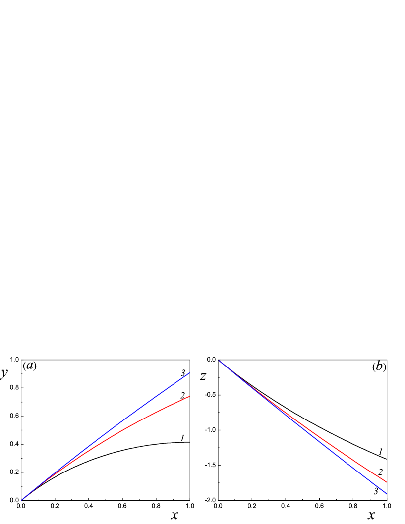
Figure 1: Dependencies of: (​a) the modulus of the pair anomalous correlation function $y=\overline{\tau}/n$ and (​b) the parameter $z$, determining the chemical potential $\mu=nU_{0}(z+2)$, on the relative density of the single-particle condensate $x=\overline{\eta}^{2}\big{/}n$ at: (1) $w=1$ , (2) $w=3$, (3) $w=10$.

We note also that in the presence of the Bose-Einstein condensate the dependence of macroscopic quantities, in particular energy, on the magnitude of interaction is, generally speaking, non-analytical. Therefore, the passage to the limit $U_{0}\rightarrow 0$ on the interaction constant in such systems is incorrect. This issue is discussed in more detail in work R35 .

V Spectrum of elementary excitations

Let us consider the propagation of small perturbations in a spatially homogeneous system. Assuming

$$\begin{array}[]{ccc}\displaystyle{\eta(r,t)=\overline{\eta}+\delta\eta(r,t),\qquad\tau(r,t)=\overline{\tau}+\delta\tau(r,t),\qquad g(r,t)=g+\delta g(r,t),}\end{array}$$ (41)

and denoting for convenience $\delta\varphi(r,t)\equiv\overline{\eta}\delta\eta(r,t)$, with an appropriate choice of phases of the complex functions in the equilibrium state from (23) – (25) we can obtain a system of linearized equations for the fluctuations $\delta\varphi(r,t),\,\delta\tau(r,t),\,\delta g(r,t)$. It is more convenient, however, to pass from the complex quantities $\delta\varphi(r,t),\,\delta\tau(r,t)$ to real variables:

$$\begin{array}[]{ccc}\displaystyle{\delta\Psi(r,t)=\delta\varphi(r,t)+\delta\varphi^{*}(r,t),\qquad\delta\Phi(r,t)=i\big{[}\delta\varphi(r,t)-\delta\varphi^{*}(r,t)\big{]},\vspace{2mm}}\\ \displaystyle{\delta\Theta(r,t)=\delta\tau(r,t)+\delta\tau^{*}(r,t),\qquad\delta\Lambda(r,t)=i\big{[}\delta\tau(r,t)-\delta\tau^{*}(r,t)\big{]}.}\end{array}$$ (42)

Fluctuations of the particle number density in the single-particle condensate $\delta n_{Q}$ and the total particle number density $\delta n$ are given by the expressions:

$$\begin{array}[]{ccc}\displaystyle{\delta n_{Q}(r,t)=\delta\Psi(r,t),\qquad\delta n(r,t)=\delta\Psi(r,t)+\delta g(r,t).}\end{array}$$ (43)

In the real variables (42) the system of linearized equations takes the form

$$\begin{array}[]{ccc}\displaystyle{\hbar\,\delta\dot{\Psi}(r)=\frac{\hbar^{2}}{2m}\Delta\delta\Phi(r)-U_{0}(\overline{\tau}-g)\delta\Phi(r)-(g+\overline{\tau})\int\!dr^{\prime\prime}U\big{(}|r-r^{\prime\prime}|\big{)}\delta\Phi(r^{\prime\prime})-\vspace{2mm}}\\ \displaystyle{-\,\overline{\eta}^{2}\int\!dr^{\prime\prime}U\big{(}|r-r^{\prime\prime}|\big{)}\delta\Lambda\Big{(}\frac{r+r^{\prime\prime}}{2}\Big{)},}\end{array}$$ (44)

$$\begin{array}[]{ccc}\displaystyle{\hbar\,\delta\dot{\Phi}(r)=-\frac{\hbar^{2}}{2m}\Delta\delta\Psi(r)+U_{0}(\overline{\tau}-g)\delta\Psi(r)\,+\vspace{2mm}}\\ \displaystyle{+\big{(}2\overline{\eta}^{2}+g-\overline{\tau})\int\!dr^{\prime\prime}U\big{(}|r-r^{\prime\prime}|\big{)}\delta\Psi(r^{\prime\prime})+\,\overline{\eta}^{2}\int\!dr^{\prime\prime}U\big{(}|r-r^{\prime\prime}|\big{)}\delta\Theta\Big{(}\frac{r+r^{\prime\prime}}{2}\Big{)}\,+\vspace{2mm}}\\ \displaystyle{+\,2\overline{\eta}^{2}\int\!dr^{\prime\prime}U\big{(}|r-r^{\prime\prime}|\big{)}\delta g\Big{(}\frac{r+r^{\prime\prime}}{2}\Big{)}+2\overline{\eta}^{2}\int\!dr^{\prime\prime}U\big{(}|r-r^{\prime\prime}|\big{)}\delta g\big{(}r^{\prime\prime}\big{)},}\end{array}$$ (45)

$$\begin{array}[]{ccc}\displaystyle{\hbar\,\delta\dot{g}(r)=\int\!dr^{\prime\prime}U\big{(}|r-r^{\prime\prime}|\big{)}\bigg{\{}g\big{[}\delta\Phi(r^{\prime\prime})-\delta\Phi(r)\big{]}+\overline{\eta}^{2}\delta\Lambda\Big{(}\frac{r+r^{\prime\prime}}{2}\Big{)}+\overline{\tau}\delta\Phi(r)+\overline{\tau}\delta\Phi(r^{\prime\prime})\bigg{\}},}\end{array}$$ (46)

$$\begin{array}[]{ccc}\displaystyle{\hbar\,\delta\dot{\Lambda}(r)=-\frac{\hbar^{2}}{4m}\Delta\delta\Theta(r)\,+\vspace{2mm}}\\ \displaystyle{+\big{[}U(0)+2U_{0}(\overline{\tau}-g)\big{]}\delta\Theta(r)+2\big{(}\overline{\eta}^{2}+2g\big{)}\int\!dr^{\prime\prime}U\big{(}|r-r^{\prime\prime}|\big{)}\delta\Theta\Big{(}\frac{r+r^{\prime\prime}}{2}\Big{)}\,+\vspace{2mm}}\\ \displaystyle{+2\big{[}U(0)+U_{0}(-\overline{\tau}+g)\big{]}\delta\Psi(r)+2\big{(}-3\overline{\tau}+g\big{)}\int\!dr^{\prime\prime}U\big{(}|r-r^{\prime\prime}|\big{)}\delta\Psi\big{(}r^{\prime\prime}\big{)}\,-\vspace{2mm}}\\ \displaystyle{-4\tau\int\!dr^{\prime\prime}U\big{(}|r-r^{\prime\prime}|\big{)}\delta g\big{(}r^{\prime\prime}\big{)}+4\big{(}\overline{\eta}^{2}-2\overline{\tau}\big{)}\int\!dr^{\prime\prime}U\big{(}|r-r^{\prime\prime}|\big{)}\delta g\Big{(}\frac{r+r^{\prime\prime}}{2}\Big{)},}\end{array}$$ (47)

$$\begin{array}[]{ccc}\displaystyle{\hbar\,\delta\dot{\Theta}(r)=\frac{\hbar^{2}}{4m}\Delta\delta\Lambda(r)-2\big{[}U(0)+U_{0}(-\overline{\tau}+g)\big{]}\delta\Phi(r)\,-\vspace{2mm}}\\ \displaystyle{-2\big{(}-\overline{\tau}+g)\int\!dr^{\prime\prime}U\big{(}|r-r^{\prime\prime}|\big{)}\delta\Phi(r^{\prime\prime})-4\overline{\tau}\int\!dr^{\prime\prime}U\big{(}|r-r^{\prime\prime}|\big{)}\delta\Phi(r^{\prime\prime})\,-\vspace{2mm}}\\ \displaystyle{-\big{[}U(0)+2U_{0}(\overline{\tau}-g)\big{]}\delta\Lambda(r)-2\big{(}\overline{\eta}^{2}+2g\big{)}\int\!dr^{\prime\prime}U\big{(}|r-r^{\prime\prime}|\big{)}\delta\Lambda\Big{(}\frac{r+r^{\prime\prime}}{2}\Big{)}.}\end{array}$$ (48)

We assume that the dependences of fluctuations on coordinates and time have the form $\sim\exp\!\!\big{[}i({\bf k}{\bf r}-\omega t)\big{]}$ and represent the Fourier component of the interaction potential $U_{k}=\!\int d{\bf r}U(|{\bf r}|)e^{i{\bf k}{\bf r}}$ in the form $U_{k}=U_{0}+\Delta U_{k}$, separating the part $\Delta U_{k}\equiv\!\int d{\bf r}U(|{\bf r}|)\big{(}e^{i{\bf k}{\bf r}}-1\big{)}$ that depends on the wave vector. Then, taking into account the notations (35), (36), we arrive at a system of homogeneous linear algebraic equations:

$$\begin{array}[]{ccc}\displaystyle{i\hbar\,\omega\delta\Phi=-\big{[}\varepsilon_{k}+n\Delta U_{k}(1+z+2x)+2xnU_{0}\big{]}\delta\Psi\,-\vspace{3mm}}\\ \displaystyle{-\,xn(U_{0}+\Delta U_{k/2})\delta\Theta-2xn\big{[}2U_{0}+(\Delta U_{k}+\Delta U_{k/2})\big{]}\delta g,}\end{array}$$ (49)

$$\begin{array}[]{ccc}\displaystyle{i\hbar\,\omega\delta\Lambda=-\bigg{[}\frac{\varepsilon_{k}}{2}+2n\Delta U_{k/2}(2-x)+2nU_{0}(2w-z-x)\bigg{]}\delta\Theta\,-\vspace{3mm}}\\ \displaystyle{-2\big{[}2nU_{0}(2w+2z+x)+n\Delta U_{k}(2x+3z+1)\big{]}\delta\Psi\,-\vspace{3mm}}\\ \displaystyle{-4\big{[}nU_{0}(4x+3z)+n\Delta U_{k}(x+z)+n\Delta U_{k/2}(3x+2z)\big{]}\delta g,}\end{array}$$ (50)

$$\begin{array}[]{ccc}\displaystyle{i\hbar\,\omega\delta\Psi=\big{[}\varepsilon_{k}+n\Delta U_{k}(1-z-2x)-2nU_{0}(z+x)\big{]}\delta\Phi+xn\big{(}U_{0}+\Delta U_{k/2}\big{)}\delta\Lambda,}\end{array}$$ (51)

$$\begin{array}[]{ccc}\displaystyle{i\hbar\,\omega\delta\Theta=\bigg{[}\frac{\varepsilon_{k}}{2}+2n\Delta U_{k/2}(2-x)+2nU_{0}(2w-z-x)\bigg{]}\delta\Lambda\,+\vspace{3mm}}\\ \displaystyle{+2\big{[}2nU_{0}(2w-x)+n\Delta U_{k}(1-2x-z)\big{]}\delta\Phi,}\end{array}$$ (52)

$$\begin{array}[]{ccc}\displaystyle{i\hbar\,\omega\delta g=\big{[}2nU_{0}(x+z)-n\Delta U_{k}(1-2x-z)\big{]}\delta\Phi-xn\big{(}U_{0}+\Delta U_{k/2}\big{)}\delta\Lambda.}\end{array}$$ (53)

Here $\varepsilon_{k}=\hbar^{2}k^{2}\big{/}2m$ is the energy of a free particle. The fluctuations $\delta\Psi,\,\delta\Theta,\,\delta g$ in (51) – (53) can be expressed in terms of the fluctuations of quantities $\delta\Phi$ and $\delta\Lambda$, for which we obtain a system of linear equations

$$\begin{array}[]{ccc}\displaystyle{(\hbar\omega)^{2}\delta\Phi=A_{k}\delta\Phi+B_{k}\delta\Lambda,\vspace{3mm}}\\ \displaystyle{(\hbar\omega)^{2}\delta\Lambda=C_{k}\delta\Lambda+D_{k}\delta\Phi.}\end{array}$$ (54)

The coefficients $A_{k},\,B_{k},\,C_{k},\,D_{k}$ entering here have a rather cumbersome form, and they are given in Appendix A. From the system of linear equations (54) there follows the dispersion equation

$$\begin{array}[]{ccc}\displaystyle{(\hbar\omega)^{4}-L_{k}(\hbar\omega)^{2}+N_{k}=0,}\end{array}$$ (55)

where $L_{k}\equiv A_{k}+C_{k}$ and $N_{k}\equiv A_{k}C_{k}-B_{k}D_{k}$. From (55) we find that there are two branches of elementary excitations

$$\begin{array}[]{ccc}\displaystyle{\hbar\omega_{k}^{(\pm)}=\sqrt{\frac{1}{2}\left(L_{k}\pm\sqrt{L_{k}^{2}-4N_{k}}\right)}.}\end{array}$$ (56)

Since, as the calculation shows, $N_{0}=0$, the solution $\omega_{k}^{(-)}$ describes sound excitations, whose energy tends linearly in $k$ to zero in the long wavelength limit. The solution $\omega_{k}^{(+)}$ describes optical excitations, whose energy $\hbar\omega_{0}^{(+)}=\sqrt{L_{0}}$ is finite at $k=0$. Note that the propagation of excitations of both types is accompanied by the density fluctuations, so that they can be detected, as it actually takes place in reality, in neutron scattering experiments R13 ; R14 ; R15 ; R16 ; R17 ; R18 ; R19 ; R20 .

In order for the excitations to be undamped, the obvious condition must hold $L_{k}^{2}-4N_{k}\geq 0$. If also $L_{k}>0$, then the excitations of the optical branch are undamped for all $k$, and the excitations of the sound branch remain undamped when the condition $N_{k}\geq 0$ holds. In what follows, we will consider only the case $L_{k}>0$, as it takes place in the system under consideration.

VI Dispersion curves for the modified Sutherland potential

Let us analyze the form of dispersion curves in case of interaction of particles with the potential (26). In this case

$$\begin{array}[]{ccc}\displaystyle{U_{0}=\upsilon_{a}I(1-J),\vspace{3mm}}\\ \displaystyle{\Delta U_{k}\equiv U_{k}-U_{0}\equiv 3\upsilon_{a}If(\kappa),}\end{array}$$ (57)

where the function

$$\begin{array}[]{ccc}\displaystyle{f(\kappa)\equiv g(\kappa)-\frac{J}{4}\,q(\kappa)}\end{array}$$ (58)

is expressed through the functions

$$\begin{array}[]{ccc}\displaystyle{g(\kappa)\equiv\frac{(\sin\kappa-\kappa\cos\kappa)}{\kappa^{3}}-\frac{1}{3},\vspace{3mm}}\\ \displaystyle{q(\kappa)\equiv\frac{\sin\kappa}{\kappa}+\frac{1}{3}\cos\kappa-\frac{\kappa}{6}\sin\kappa-\frac{\kappa^{2}}{6}\cos\kappa+\frac{\kappa^{3}}{6}\bigg{(}\frac{\pi}{2}-\int_{0}^{\kappa}\frac{\sin y}{y}\,dy\bigg{)}-\frac{4}{3}.}\end{array}$$ (59)

Here the notation $\kappa\equiv kr_{0}$ is introduced. The function $q(\kappa)$ describes the influence of the attractive part of the potential on the shape of dispersion curves. At $\kappa=0$ the functions (58), (59) turn to zero, and at small wave numbers $\kappa\ll 1$:

$$\begin{array}[]{ccc}\displaystyle{g(\kappa)\approx-\frac{\kappa^{2}}{30},\qquad q(\kappa)\approx-\frac{2}{3}\,\kappa^{2},\qquad f(\kappa)\approx\frac{1}{6}\left(J-\frac{1}{5}\right)\!\kappa^{2}.}\end{array}$$ (60)

As we can see, there is a critical value of the parameter $J_{*}=1/5$  at which the function $f(\kappa)$ changes sign at small values of $\kappa$. In the opposite case $\kappa\gg 1$:

$$\begin{array}[]{ccc}\displaystyle{g(\kappa)=-\frac{1}{3},\qquad q(\kappa)=-\frac{4}{3},\qquad f(\kappa)=-\frac{1}{3}(1-J)\equiv-\frac{1}{3b}.}\end{array}$$ (61)

In this limit the optical branch goes over to the dispersion law of a free particle, and the sound branch to the dispersion law of a particle with a doubled mass:

$$\begin{array}[]{ccc}\displaystyle{\hbar\omega_{k}^{(+)}=\frac{\hbar^{2}k^{2}}{2m},\qquad\hbar\omega_{k}^{(-)}=\frac{\hbar^{2}k^{2}}{4m}.}\end{array}$$ (62)

In numerical calculations it is more convenient to use the dimensionless form of coefficients of the dispersion equation:

$$\begin{array}[]{ccc}\displaystyle{\tilde{A}_{k}\equiv A_{k}\big{/}(nU_{0})^{2},\quad\tilde{B}_{k}\equiv B_{k}\big{/}(nU_{0})^{2},\quad\tilde{C}_{k}\equiv C_{k}\big{/}(nU_{0})^{2},\quad\tilde{D}_{k}\equiv D_{k}\big{/}(nU_{0})^{2},\vspace{3mm}}\\ \displaystyle{\tilde{L}_{k}\equiv L_{k}\big{/}(nU_{0})^{2}=\tilde{A}_{k}+\tilde{C}_{k},\quad\tilde{N}_{k}\equiv N_{k}\big{/}(nU_{0})^{4}=\tilde{A}_{k}\tilde{C}_{k}-\tilde{B}_{k}\tilde{D}_{k}.}\end{array}$$ (63)

Explicit expressions of the coefficients of the dispersion equation (55) for the potential (26) are given in Appendix B. In terms of dimensionless quantities the dispersion laws (56) can be written as

$$\begin{array}[]{ccc}\displaystyle{\varepsilon_{k}^{(\pm)}\equiv\frac{\hbar\omega_{k}^{(\pm)}}{nU_{0}}=\sqrt{\frac{1}{2}\left(\tilde{L}_{k}\pm\sqrt{\tilde{L}_{k}^{2}-4\tilde{N}_{k}}\right)}.}\end{array}$$ (64)

In the long wavelength limit $\kappa\ll 1$, the expansions are valid: $\tilde{A}_{k}\approx\tilde{A}_{0}+\tilde{A}_{2}\kappa^{2}$,  $\tilde{B}_{k}\approx\tilde{B}_{0}+\tilde{B}_{2}\kappa^{2}$,  $\tilde{C}_{k}\approx\tilde{C}_{0}+\tilde{C}_{2}\kappa^{2}$,  $\tilde{D}_{k}\approx\tilde{D}_{0}+\tilde{D}_{2}\kappa^{2}$. The coefficients of these expansions are given in Appendix C. In this limit the dispersion laws for the sound and optical branches take the form

$$\begin{array}[]{ccc}\displaystyle{\omega_{k}^{(-)}=ck,\qquad\omega_{k}^{(+)}=\omega_{0}+\alpha k^{2},\vspace{-2mm}}\end{array}$$ (65)

or

$$\begin{array}[]{ccc}\displaystyle{\varepsilon_{k}^{(-)}=\tilde{c}\kappa,\qquad\varepsilon_{k}^{(+)}=\varepsilon_{0}+\tilde{\alpha}\kappa^{2},}\end{array}$$ (66)

where $c$ is the speed of sound, $\omega_{0}$ is the gap in the optical branch. The corresponding dimensionless parameters in (66) are:

$$\begin{array}[]{ccc}\displaystyle{\tilde{c}\equiv\frac{\hbar}{nU_{0}r_{0}}\,c,\qquad\varepsilon_{0}\equiv\frac{\hbar\omega_{0}}{nU_{0}},\qquad\tilde{\alpha}\equiv\frac{\hbar}{nU_{0}r_{0}^{2}}\,\alpha.}\end{array}$$ (67)

With allowance for introduced notations of dimensionless quantities, the speed of sound, the frequency of homogeneous oscillations and the coefficient in the optical branch are determined by the formulas:

$$\begin{array}[]{ccc}\displaystyle{\tilde{c}=\sqrt{\frac{\tilde{A}_{0}\tilde{C}_{2}+\tilde{C}_{0}\tilde{A}_{2}-\tilde{B}_{0}\tilde{D}_{2}-\tilde{D}_{0}\tilde{B}_{2}}{\tilde{A}_{0}+\tilde{C}_{0}}},\qquad\varepsilon_{0}=\sqrt{\tilde{A}_{0}+\tilde{C}_{0}},\vspace{3mm}}\\ \displaystyle{\tilde{\alpha}=\frac{\big{(}\tilde{A}_{0}\tilde{A}_{2}+\tilde{C}_{0}\tilde{C}_{2}+\tilde{B}_{0}\tilde{D}_{2}+\tilde{D}_{0}\tilde{B}_{2}\big{)}}{2\big{(}\tilde{A}_{0}+\tilde{C}_{0}\big{)}^{3/2}}.}\end{array}$$ (68)

In numerical calculations we will fix the parameters of the potential: the radius of the repulsive core $r_{0}$, the parameters $J$ or $b=1/(1-J)$, and the parameter $\theta\equiv I/\varepsilon_{a}$ determining the intensity of particle repulsion at small distances. The system density $n$ is assumed to be known. Then $\displaystyle{nU_{0}=\varepsilon_{a}\frac{\chi\theta}{b}}$, where recall that $\displaystyle{\varepsilon_{a}\equiv\frac{\hbar^{2}}{2mr_{0}^{2}}}$  and $\chi\equiv n\upsilon_{a}$.

Dense system. Consider first a dense system with parameters close to those of liquid helium-4: $m=6.65\cdot\!10^{-24}$ g,  $n=2.2\cdot\!10^{22}$ cm^-3. We take the radius of the core $r_{0}=2.24\cdot\!10^{-8}$ cm, so that in this case $\chi\approx 1$ and $\varepsilon_{a}=1.67\cdot\!10^{-16}$ erg$\,\,\approx 1.2$ K. Other parameters of the potential (26) are set as follows: $\theta=100$  and $J=0.1$. In accordance with the experimental data on neutron scattering R20 ; R34 , we consider $x\approx 0.1$. With the chosen fitting parameters, we obtain the following numerical values of the sound speed, the frequency of homogeneous oscillations and the coefficient in the optical branch:

$$\begin{array}[]{ccc}\displaystyle{c=4.3\cdot\!10^{4}\,{\rm cm}\!\cdot{\rm s}^{-1},\qquad\frac{\omega_{0}}{2\pi}=7.8\cdot\!10^{12}\,{\rm s}^{-1},\qquad\alpha=-3.7\cdot\!10^{-4}\,{\rm cm}^{2}\!\cdot{\rm s}^{-1}.}\end{array}$$

The used set of parameters leads to the velocity of phonons that somewhat exceeds the velocity of the low-frequency hydrodynamic first sound in superfluid helium $c_{1}=2.3\cdot\!10^{4}\,{\rm cm}\!\cdot{\rm s}^{-1}$. The numerically calculated dispersion curves in a superfluid liquid are shown in Fig. 2.

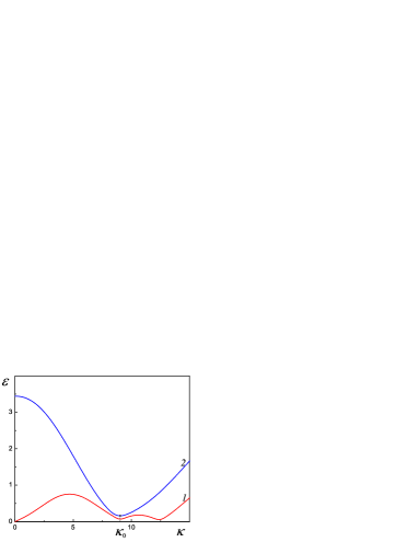
Figure 2: Phonon (​1) $\varepsilon=\big{(}\hbar\omega^{(-)}\!\big{/}nU_{0}\big{)}$ and optical (​2) $\varepsilon=\big{(}\hbar\omega^{(+)}\!\big{/}nU_{0}\big{)}$ branches in the dense system with $n=2.2\cdot\!10^{22}$ cm^-3 and parameters: $m=6.65\cdot\!10^{-24}$ g,  $r_{0}=2.24\cdot\!10^{-8}$ cm,  $x=0.1$,  $\chi=1$,  $\theta=100$,  $J=0.1$.

The lower curve describes the sound excitations in the long wavelength limit and it has the roton-like minimum at a certain value of the wave number. Within the framework of the nonlocal Gross-Pitaevskii equation, in the case when pair correlations are not taken into account, a similar nonmonotonic curve was obtained in R36 . The appearance of the upper curve with a gap in the limit $k\rightarrow 0$  is a consequence of taking into account pair correlations, and it also has the roton-like minimum at $\kappa_{0}$ close to the minimum on the sound branch.

Rarefied system. With a decrease in the density and, consequently, with an increase in the average distance between particles, the effect of taking into account the finite radius of the interaction potential on the shape of the excitation spectrum is weakened. At a certain density $\chi_{0}$ the parameter $\alpha$ in the optical branch of the spectrum (65) changes sign, becoming positive at $\chi<\chi_{0}$. The value of $\chi_{0}$ is determined from the condition that the numerator in the formula for $\tilde{\alpha}$ (68) turns to zero. For the chosen above values of the potential parameters and $x=1$ it is equal to $\chi_{0}\approx 0.1695$, which corresponds to the density $n_{0}=3.6\cdot\!10^{21}$ cm^-3. For $x=0.1$ these values are equal to $\chi_{0}\approx 0.1004$, and $n_{0}=2.1\cdot\!10^{21}$ cm^-3. The dispersion curves for the density $n=10^{15}$ cm^-3 close to that achieved in atomic gases and the same parameters and the mass of particles as above are shown in Fig. 3.

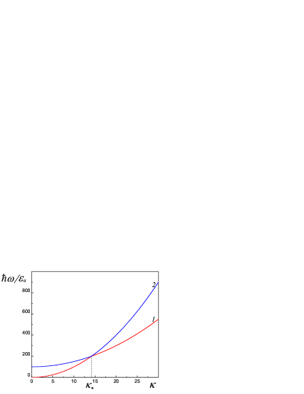
Figure 3: Phonon (​1) $\varepsilon=\hbar\omega^{(-)}\!\big{/}\varepsilon_{a}$ and optical (​2) $\varepsilon=\hbar\omega^{(+)}\!\big{/}\varepsilon_{a}$ branches in the rarefied system with $n=10^{15}$ cm^-3 and parameters: $m=6.65\cdot\!10^{-24}$ g,  $r_{0}=2.24\cdot\!10^{-8}$ cm,  $x=1$,  $\chi=4.7\cdot\!10^{-8}$,  $\theta=100$,  $J=0.1$.

The shape of this spectrum is close to that previously obtained in R11 for the local interaction. At low densities the energy on both branches increases monotonically and at $\kappa_{*}\approx 14.142$ the branches approach each other so strongly that, apparently, the transformation of phonon excitations into optical ones and vice versa becomes possible here. This question is of independent interest, but is beyond the scope of this work.

VII Dispersion of sound

In the limit $k\rightarrow 0$ for the phonon branch, the energy depends linearly on the wave number $\varepsilon_{k}^{(-)}\!=\tilde{c}\kappa$. With increasing $k$ this dependence deviates from linearity. If the deviation is towards lower energies then one speaks of a normal dispersion, and if it is towards higher energies – of an anomalous dispersion. At very low frequencies the speed of sound is equal to the speed of the hydrodynamic first sound. At higher frequencies $\omega\gg\nu$, where $\nu$ is the collision frequency, there is a transition to the zero-sound mode. The phase velocity of the zero sound in quantum liquids turns out to be greater than the phase velocity of the first sound R37 . It should also be noted that the sound part of the spectrum is practically insensitive to the superfluid transition.

Accounting for the deviation of the sound dispersion law from a linear dependence is important, in particular, for studying kinetic processes in superfluid ⁴He. In early works on the kinetics of helium it was assumed that the deviation from a linear dependence occurs in direction of decreasing energy (the normal dispersion) R12 . Subsequently, precision measurements of the initial part of the dispersion curve revealed the deviation of the phase velocity of excitations towards larger values (an anomalous dispersion) R19 ; R38 . The calculation carried out in this work also leads to an anomalous dispersion. The phonon branch and its comparison with the sound linear dependence are shown in Fig. 4.

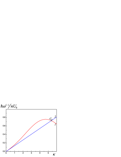
Figure 4: Dispersion of phonons. Coordinates of the point of intersection of the phonon branch with the linear dependence $C_{*}(5.36,\,0.724)$.

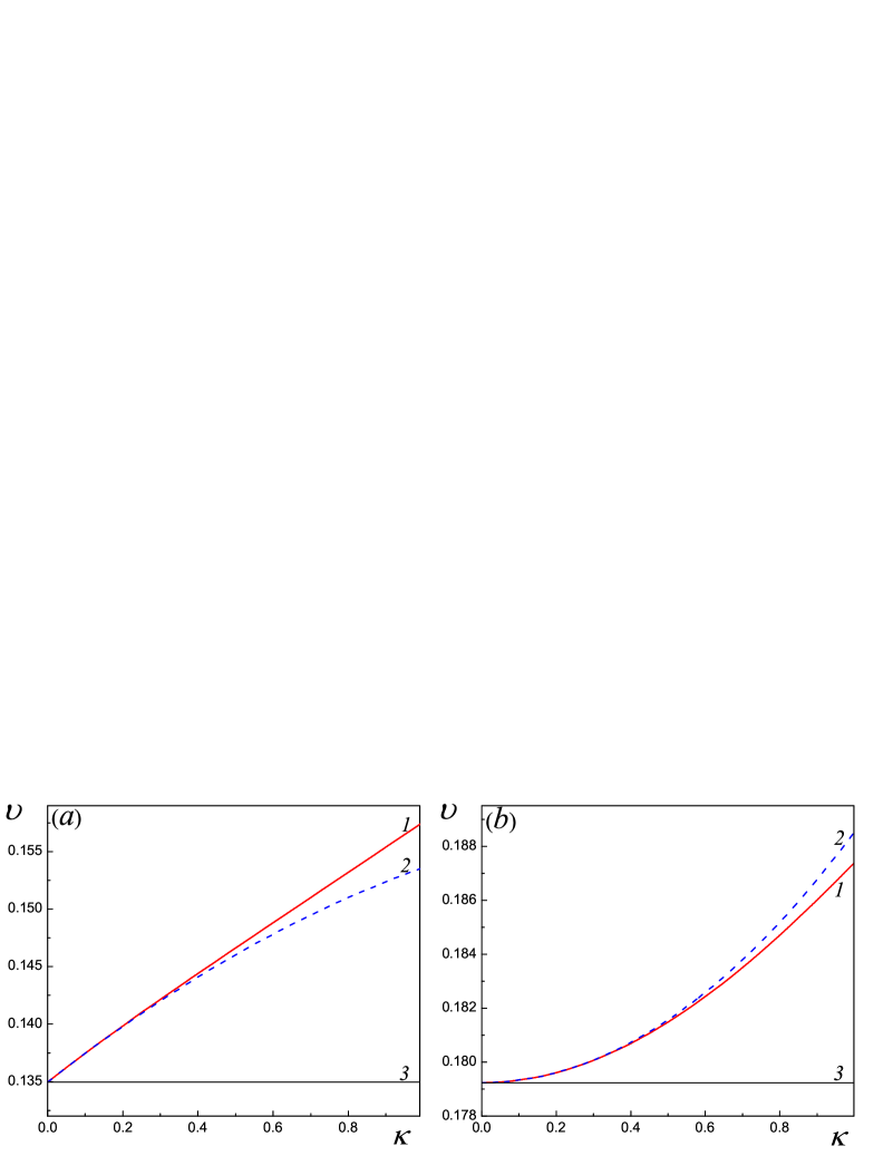
Figure 5: (​1) The exact phase velocity $\upsilon_{ph}(\kappa)$; (​2) the phase velocity $\upsilon_{ph}^{(2)}(\kappa)$ according to formula (69); (​3) the phase velocity without account of dispersion $\upsilon_{ph}^{(0)}$. (​a) Calculation with parameters $\theta=100,\,J=0.1,\,x=0.1,\,\chi=1;\,\upsilon_{ph}^{(0)}=0.135$. (​b) Calculation with parameters $\theta=100,\,J=0.0,\,x=0.1,\,\chi=1;\,\upsilon_{ph}^{(0)}=0.179$.

As we can see, the phonon branch deviates from the linear dependence towards higher energies and crosses the linear dependence at point $C_{*}$. Using the expansions of coefficients given in Appendix C, for the phase velocity to within a quadratic correction we obtain the following formula:

$$\begin{array}[]{ccc}\displaystyle{\upsilon_{ph}(\kappa)\equiv\frac{\hbar}{nU_{0}r_{0}}\frac{\omega^{(-)}}{k}=\sqrt{\frac{\tilde{N}_{2}}{\tilde{L}_{0}}}\,+\frac{\tilde{N}_{3}}{2\sqrt{\tilde{L}_{0}\tilde{N}_{2}}}\,\kappa\,\,+\frac{\big{(}4\tilde{L}_{0}^{2}\tilde{N}_{2}\tilde{N}_{4}-4\tilde{L}_{0}\tilde{L}_{2}\tilde{N}_{2}^{2}+4\tilde{N}_{2}^{3}-\tilde{L}_{0}^{2}\tilde{N}_{3}^{2}\big{)}}{8\tilde{L}_{0}^{5/2}\tilde{N}_{2}^{3/2}}\,\kappa^{2}.}\end{array}$$ (69)

Dependences of the phase velocity on the wave number are shown in Fig. 5. Here curve 1 corresponds to the exact phase velocity $\upsilon_{ph}(\kappa)$, curve 2 corresponds to the phase velocity calculated by formula (69), and line 3 – to the phase velocity in the absence of dispersion.

It draws attention that the linear contribution in the expression for the phase velocity (69) exists only when the attraction in the interparticle potential is taken into account (Fig. 5a). In the model of “semi-transparent sphere”, when there is no attraction $(J=0)$, the linear term in (69) vanishes (Fig. 5b).

VIII Discussion. Conclusions

In his first work on the theory of superfluid helium R39 , Landau suggested that there are two types of elementary excitations in it – the sound excitations and those that have a gap at zero momentum. However, it turned out that the excitations with a gap make an insufficient contribution for a correct description of thermodynamic quantities. In this connection Landau proposed in R40 his famous unified nonmonotonic dispersion curve. For such law of dispersion the main contribution to thermodynamic quantities comes from the gapless excitations at small momenta (phonons) and the excitations with a large momentum near the minimum of the dispersion curve (rotons).

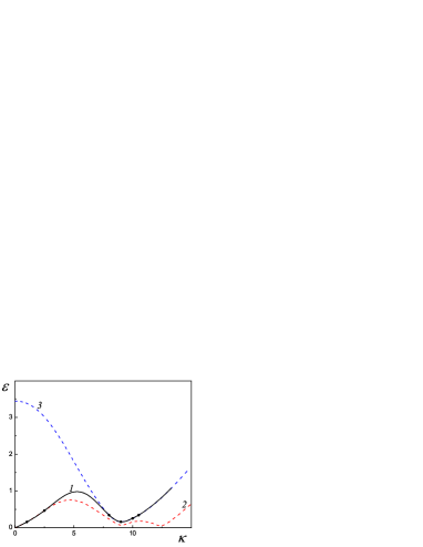
Figure 6: Formation of the unified spectrum $\varepsilon_{a}(\kappa)$ (curve ​1) from (​2) the phonon $\varepsilon_{ph}(\kappa)=\big{(}\hbar\omega^{(-)}\!\big{/}nU_{0}\big{)}$ and (​3) the optical-roton $\varepsilon_{o\!p}(\kappa)=\big{(}\hbar\omega^{(+)}\!\big{/}nU_{0}\big{)}$ branches. Calculation parameters: $n=2.2\cdot\!10^{22}$ cm^-3, $m=6.65\cdot\!10^{-24}$ g, $r_{0}=2.24\cdot\!10^{-8}$ cm,  $x=0.1,\,\chi=1,\,\theta=100,\,J=0.1$.

The shape of the curve in helium was experimentally studied and analyzed in experiments on neutron scattering R13 ; R14 ; R15 ; R16 ; R17 ; R18 ; R19 ; R20 . These experiments point to the complex structure of the spectrum. The scattering peaks observed in experiments can be characterized by their total intensity $Z(q)$ and width at half maximum $W(q)$. These characteristics behave differently in different regions of change of the transmitted wave number $q$. A sharp peak is observed in the region $0<q<0.65\,\textrm{{\AA}}^{-1}$, corresponding to the weakly damped sound excitations. Upon transition to the maxon-roton region $q>0.65\,\textrm{{\AA}}^{-1}$ the behavior of the characteristics $Z(q)$ and $W(q)$ changes significantly, which indicates the probable different nature of the sound and maxon-roton regions of the dispersion curve.

The scattering peak has the most complex structure in the transition region R17 ; R18 ; R19 ; R20 . Here the sound component gradually becomes strongly damped, but a narrow component appears, associated with the maxon-roton excitations. In addition, apparently, there is also a broad component. When processing the experimental data of experiments R17 ; R18 ; R19 ; R20 , it was possible to distinguish two components in the neutron scattering peak in the maxon-roton region – narrow and wide. At low temperature the narrow peak lies somewhat higher than the broad peak R17 .

The calculations of dispersion curves performed in this work and the results of experiments on neutron scattering R13 ; R14 ; R15 ; R16 ; R17 ; R18 ; R19 ; R20 give grounds to assume that the Landau curve consists of two parts that belong to two different excitation branches. The initial region of the spectrum is determined by the long-lived phonon excitations, which become strongly damped at large wave numbers. Well-defined long-lived excitations in the maxon-roton region of the spectrum are a part of the optical excitation branch. Since in the theoretical model considered in this work there were made a number of significant approximations, which were mentioned above, then the constructed dispersion curves are not accurate. Nevertheless, the obtained results allow to propose a qualitative picture of formation of the unified spectrum from two different excitation branches, which is shown in Fig. 6.

The interpolation curve in Fig. 6 is given by the formula

$$\begin{array}[]{ccc}\displaystyle{\varepsilon_{a}(\kappa)=\tilde{c}\kappa+\kappa\,\psi(\kappa),}\end{array}$$ (70)

where $\psi(\kappa)$ is a polynomial constructed using the Lagrange interpolation formula on the basis of several points on the phonon and optical branches shown in Fig. 6. It should be noted that excitations on the optical branch at small momenta are difficult to detect experimentally, since they make a negligibly small contribution to thermodynamic quantities, and it is technically difficult to measure excitations with small momenta in neutron scattering experiments.

The main results of the work are the following: (a) The system of equations for the single-particle condensate and pair correlations is obtained with taking into account the finite radius of the interaction potential between particles. (b) The spectrum of elementary excitations is studied and it is shown that it has two branches – phonon and optical. At high densities the dispersion curves are nonmonotonic and have the roton-like minima. (c) It is shown that the phonon spectrum has an anomalous dispersion. (d) On the basis of the performed calculations and analysis of experiments on inelastic neutron scattering, an assumption is made about the complex nature of the Landau spectrum in superfluid ⁴He.

Appendix A General form of coefficients in the dispersion equation (55)

$$\begin{array}[]{ccc}\displaystyle{L_{k}\equiv A_{k}+C_{k},\qquad N_{k}\equiv A_{k}C_{k}-B_{k}D_{k},}\end{array}$$

$$\begin{array}[]{ccc}\displaystyle{A_{k}=\Big{[}\varepsilon_{k}^{(1)}+2xnU_{0}\Big{]}\!\Big{[}\varepsilon_{k}^{(2)}-2nU_{0}(x+z)\Big{]}+\vspace{2mm}}\\ \displaystyle{\hskip 28.45274pt+\,2xn\big{(}U_{0}+\Delta U_{k/2}\big{)}\big{[}2nU_{0}(2w-x)+\alpha_{k}\big{]}+\vspace{2mm}}\\ \displaystyle{\hskip 62.59605pt+\,2xn\big{[}2U_{0}+\big{(}\Delta U_{k}+\Delta U_{k/2}\big{)}\big{]}\!\big{[}2nU_{0}(x+z)-\alpha_{k}\big{]},}\end{array}$$ (71)

$$\begin{array}[]{ccc}\displaystyle{B_{k}=xn\big{(}U_{0}+\Delta U_{k/2}\big{)}\Big{[}\varepsilon_{k}^{(1)}+\,\varepsilon_{k}^{(3)}+2nU_{0}(2w-z-2x)-2xn\big{(}\Delta U_{k}+\Delta U_{k/2}\big{)}\Big{]},}\end{array}$$ (72)

$$\begin{array}[]{ccc}\displaystyle{C_{k}=\Big{[}\varepsilon_{k}^{(3)}+2nU_{0}(2w-z-x)\Big{]}^{\!2}+2xn\big{(}U_{0}+\Delta U_{k/2}\big{)}\big{[}2nU_{0}(2w-z-3x)+\gamma_{k}-2\delta_{k}\big{]},}\end{array}$$ (73)

$$\begin{array}[]{ccc}\displaystyle{D_{k}=2\Big{[}\varepsilon_{k}^{(3)}+2nU_{0}(2w-z-x)\Big{]}\!\big{[}2nU_{0}(2w-x)+\alpha_{k}\big{]}\,+\vspace{2mm}}\\ \displaystyle{\hskip 14.22636pt+2\Big{[}\varepsilon_{k}^{(2)}-2nU_{0}(x+z)\Big{]}\!\big{[}2nU_{0}(2w+2z+x)+\gamma_{k}\big{]}\,+\vspace{2mm}}\\ \displaystyle{+\,4\big{[}nU_{0}(4x+3z)+\delta_{k}\big{]}\!\big{[}2nU_{0}(x+z)-\alpha_{k}\big{]}.}\end{array}$$ (74)

In formulas (A1) – (A4) the notation is used:

$$\begin{array}[]{ccc}\displaystyle{\alpha_{k}\equiv n\Delta U_{k}(1-2x-z),\quad\beta_{k}\equiv n\Delta U_{k}(1+2x+z),\quad\gamma_{k}\equiv n\Delta U_{k}(1+2x+3z),\vspace{3mm}}\\ \displaystyle{\hskip 14.22636pt\delta_{k}\equiv n\Delta U_{k}(x+z)+n\Delta U_{k/2}(3x+2z),\vspace{3mm}}\\ \displaystyle{\varepsilon_{k}^{(1)}\equiv\varepsilon_{k}+\beta_{k},\quad\varepsilon_{k}^{(2)}\equiv\varepsilon_{k}+\alpha_{k},\quad\varepsilon_{k}^{(3)}\equiv\frac{\varepsilon_{k}}{2}+2n\Delta U_{k/2}(2-x).}\end{array}$$ (75)

Appendix B Coefficients of the dispersion equation (55) for the potential (26)

$$\begin{array}[]{ccc}\displaystyle{\frac{A_{k}}{n^{2}U_{0}^{2}}\equiv\tilde{A}_{k}=4x(z+2w)+2b\Big{[}-\zeta z\kappa^{2}-3(x+z)(1+z)f(\kappa)+6x(z+2w)f\Big{(}\frac{\kappa}{2}\Big{)}\Big{]}\,+\vspace{2mm}}\\ \displaystyle{+\,b^{2}\Big{[}\zeta^{2}\kappa^{4}+6\zeta\kappa^{2}f(\kappa)+9(1+z)(1-2x-z)f^{2}(\kappa)\Big{]},}\end{array}$$ (76)

$$\begin{array}[]{ccc}\displaystyle{\frac{B_{k}}{n^{2}U_{0}^{2}}\equiv\tilde{B}_{k}=2x(2w-2x-z)+3bx\!\left[\frac{1}{2}\zeta\kappa^{2}+(1+z)f(\kappa)+2(2+2w-4x-z)f\Big{(}\frac{\kappa}{2}\Big{)}\right]\,+\vspace{2mm}}\\ \displaystyle{+\,9b^{2}f\Big{(}\frac{\kappa}{2}\Big{)}x\!\left[\frac{1}{2}\zeta\kappa^{2}+(1+z)f(\kappa)+4(1-x)f\Big{(}\frac{\kappa}{2}\Big{)}\right],}\end{array}$$ (77)

$$\begin{array}[]{ccc}\displaystyle{\frac{C_{k}}{n^{2}U_{0}^{2}}\equiv\tilde{C}_{k}=4\big{(}4w^{2}+2xw-4x^{2}-2wz-xz\big{)}\,+\vspace{2mm}}\\ \displaystyle{+\,2b\!\left[(2w-x-z)\zeta\kappa^{2}+3x(1+z)f(\kappa)+6\big{(}8w-4x-2xw-4x^{2}-4z-xz\big{)}f\Big{(}\frac{\kappa}{2}\Big{)}\right]\vspace{2mm}}\\ \displaystyle{+\,b^{2}\left[\frac{\zeta^{2}}{4}\kappa^{4}+6(2-x)\zeta\kappa^{2}f\Big{(}\frac{\kappa}{2}\Big{)}+72\big{(}2-2x-x^{2}-xz\big{)}f^{2}\Big{(}\frac{\kappa}{2}\Big{)}+18x(1+z)f(\kappa)f\Big{(}\frac{\kappa}{2}\Big{)}\right],}\end{array}$$ (78)

$$\begin{array}[]{ccc}\displaystyle{\frac{D_{k}}{n^{2}U_{0}^{2}}\equiv\tilde{D}_{k}=8\big{(}4w^{2}+2x^{2}-2xw-2wz+3xz\big{)}\,+\vspace{2mm}}\\ \displaystyle{+\,4b\Big{[}\Big{(}3w+2z+\frac{x}{2}\Big{)}\zeta\kappa^{2}+3\big{(}4w+6x^{2}+5xz-4xw-2wz-5x-3z\big{)}f(\kappa)\,+\vspace{2mm}}\\ \displaystyle{+\,6\big{(}4w-2x+6xw+4wz+xz\big{)}f\Big{(}\frac{\kappa}{2}\Big{)}\Big{]}+\vspace{2mm}}\\ \displaystyle{+\,3b^{2}\!\left[(3+2x+5z)\zeta\kappa^{2}f(\kappa)+6(1+z)(1-2x-z)f^{2}(\kappa)+24(1-2x-z)^{2}f(\kappa)f\Big{(}\frac{\kappa}{2}\Big{)}\right],}\end{array}$$ (79)

$$\begin{array}[]{ccc}\displaystyle{L_{k}=A_{k}+C_{k}=(nU_{0})^{2}\tilde{L}_{k},\qquad\tilde{L}_{k}=\tilde{A}_{k}+\tilde{C}_{k},\vspace{2mm}}\\ \displaystyle{N_{k}=A_{k}C_{k}-B_{k}D_{k}=(nU_{0})^{4}\tilde{N}_{k},\qquad\tilde{N}_{k}=\tilde{A}_{k}\tilde{C}_{k}-\tilde{B}_{k}\tilde{D}_{k}.}\end{array}$$ (80)

The notation is used:

$$\begin{array}[]{ccc}\displaystyle{\zeta\equiv\frac{\varepsilon_{a}}{\chi I}=\frac{1}{\theta\chi},\qquad b=\frac{1}{1-J},\qquad\kappa\equiv r_{0}k.}\end{array}$$ (81)

The function $f(\kappa)$ is defined by formulas (58), (59).

Appendix C Coefficients of the dispersion equation (55) for the potential (26)
in the long-wavelength limit $\kappa\ll 1$

$$\begin{array}[]{ccc}\displaystyle{\tilde{A}_{k}\approx\tilde{A}_{0}+\tilde{A}_{2}\kappa^{2}+\tilde{A}_{3}\kappa^{3}+\tilde{A}_{4}\kappa^{4},\qquad\tilde{B}_{k}\approx\tilde{B}_{0}+\tilde{B}_{2}\kappa^{2}+\tilde{B}_{3}\kappa^{3}+\tilde{B}_{4}\kappa^{4},\vspace{2mm}}\\ \displaystyle{\tilde{C}_{k}\approx\tilde{C}_{0}+\tilde{C}_{2}\kappa^{2}+\tilde{C}_{3}\kappa^{3}+\tilde{C}_{4}\kappa^{4},\qquad\tilde{D}_{k}\approx\tilde{D}_{0}+\tilde{D}_{2}\kappa^{2}+\tilde{D}_{3}\kappa^{3}+\tilde{D}_{4}\kappa^{4},\vspace{2mm}}\\ \displaystyle{\tilde{L}_{k}\approx\tilde{L}_{0}+\tilde{L}_{2}\kappa^{2}+\tilde{L}_{3}\kappa^{3}+\tilde{L}_{4}\kappa^{4},\vspace{2mm}}\\ \displaystyle{\tilde{L}_{0}\equiv\tilde{A}_{0}+\tilde{C}_{0},\quad\tilde{L}_{2}\equiv\tilde{A}_{2}+\tilde{C}_{2},\quad\tilde{L}_{3}\equiv\tilde{A}_{3}+\tilde{C}_{3},\quad\tilde{L}_{4}\equiv\tilde{A}_{4}+\tilde{C}_{4},\vspace{2mm}}\\ \displaystyle{\tilde{N}_{k}\approx\tilde{N}_{2}\kappa^{2}+\tilde{N}_{3}\kappa^{3}+\tilde{N}_{4}\kappa^{4},\vspace{2mm}}\\ \displaystyle{\tilde{N}_{2}\equiv\tilde{A}_{0}\tilde{C}_{2}+\tilde{C}_{0}\tilde{A}_{2}-\tilde{B}_{0}\tilde{D}_{2}-\tilde{D}_{0}\tilde{B}_{2},\vspace{2mm}}\\ \displaystyle{\tilde{N}_{3}\equiv\tilde{A}_{0}\tilde{C}_{3}+\tilde{C}_{0}\tilde{A}_{3}-\tilde{B}_{0}\tilde{D}_{3}-\tilde{D}_{0}\tilde{B}_{3},\vspace{2mm}}\\ \displaystyle{\tilde{N}_{4}\equiv\tilde{A}_{0}\tilde{C}_{4}+\tilde{C}_{0}\tilde{A}_{4}+\tilde{A}_{2}\tilde{C}_{2}-\tilde{B}_{0}\tilde{D}_{4}-\tilde{D}_{0}\tilde{B}_{4}-\tilde{B}_{2}\tilde{D}_{2}.\vspace{0mm}}\end{array}$$ (82)

Here

$$\begin{array}[]{ccc}\displaystyle{\tilde{A}_{0}=4x(2w+z),\qquad\tilde{B}_{0}=2x(2w-z-2x),\vspace{2mm}}\\ \displaystyle{\tilde{C}_{0}=4\big{(}\!-4x^{2}+4w^{2}+2xw-2wz-xz\big{)},\vspace{2mm}}\\ \displaystyle{\tilde{D}_{0}=8\big{(}\!2x^{2}+4w^{2}-2xw-2wz+3xz\big{)},}\end{array}$$ (83)

$$\begin{array}[]{ccc}\displaystyle{\tilde{A}_{2}=-2zb\zeta+u\big{(}2z^{2}+xz-2xw+2x+2z\big{)},\vspace{2mm}}\\ \displaystyle{\tilde{B}_{2}=\frac{x}{2}\big{[}3b\zeta-u(4+z+2w-4x)\big{]},\vspace{2mm}}\\ \displaystyle{\tilde{C}_{2}=2(2w-x-z)b\zeta+u\big{(}2x-8w+4z+2xw-xz+4x^{2}\big{)},\vspace{2mm}}\\ \displaystyle{\tilde{D}_{2}=4\!\left(3w+2z+\frac{x}{2}\right)\!b\zeta+4u\Big{(}6x-6w+3z+xw-6x^{2}-\frac{11}{2}xz\Big{)},}\end{array}$$ (84)

$$\begin{array}[]{ccc}\displaystyle{\tilde{A}_{3}=\frac{\pi}{32}(b-1)\big{(}4x+4z+3xz-2xw+4z^{2}\big{)},\vspace{2mm}}\\ \displaystyle{\tilde{B}_{3}=-\frac{\pi}{64}(b-1)\,x(6+3z+2w-4x),\vspace{2mm}}\\ \displaystyle{\tilde{C}_{3}=-\frac{\pi}{32}(b-1)\big{(}8w-4z+3xz-2xw-4x^{2}\big{)},\vspace{2mm}}\\ \displaystyle{\tilde{D}_{3}=-\frac{\pi}{16}(b-1)\big{(}24x^{2}-10xw+21xz-4wz-22x+20w-12z\big{)},}\end{array}$$ (85)

$$\begin{array}[]{ccc}\displaystyle{\tilde{A}_{4}=-6bb_{4}\Big{(}x+z+z^{2}+\frac{7}{8}xz-\frac{1}{4}xw\Big{)}+b^{2}\zeta^{2}-2b\zeta u+u^{2}\big{(}1-2x-2xz-z^{2}\big{)},\vspace{2mm}}\\ \displaystyle{\tilde{B}_{4}=\frac{3}{8}bb_{4}x(10+7z-4x+2w)-\frac{3}{8}ub\zeta x+\frac{u^{2}}{4}x(2+z-x),\vspace{2mm}}\\ \displaystyle{\tilde{C}_{4}=\frac{1}{4}\Big{(}b^{2}\zeta^{2}-2u(2-x)b\zeta+2u^{2}\big{(}2-x-x^{2}\big{)}+\frac{3}{4}bb_{4}\big{(}4x+8w-4z+7xz-2xw-4x^{2}\big{)},\vspace{2mm}}\\ \displaystyle{\tilde{D}_{4}=\frac{3}{2}bb_{4}\big{(}48x^{2}+41xz-26xw-12wz-42x+36w-24z\big{)}+\vspace{2mm}}\\ \displaystyle{+\,4u^{2}\big{(}1-3x-z+2x^{2}+xz\big{)}-ub\zeta(3+2x+5z).}\end{array}$$ (86)

The notation is used:

$$\begin{array}[]{ccc}\displaystyle{u\equiv\frac{(1/5-J)}{2(1-J)}=\frac{1}{2}\!\left(\!1-\frac{4}{5}\,b\right),\qquad b_{4}\equiv\frac{1}{120}\!\left(\frac{1}{7}+J\right).}\end{array}$$ (87)

References

• (1) E.P. Gross, Structure of a quantized vortex in boson systems, Nuovo Cimento 20, 454 (1961). doi:10.1007/BF02731494
• (2) L.P. Pitaevskii, Vortex lines in an imperfect Bose gas, JETP 40, 646 (1961) [Sov. Phys. JETP 13, 451 (1961)].
• (3) L. Pitaevskii, S. Stringari, Bose-Einstein condensation, Oxford University Press, 492 p. (2003).
• (4) C.H. Pethick, H. Smith, Bose-Einstein condensation in dilute gases, Cambridge University Press, 402 p. (2001).
• (5) Yu.M. Poluektov, The polarization properties of an atomic gas in a coherent state, Low Temp. Phys. 37, 986 (2011). doi:10.1063/1.3674269
• (6) N.N. Bogolyubov, Problems of dynamic theory in statistical physics, In the book: N.N. Bogolyubov, Selected works in three volumes, Vol. 2, Naukova dumka, Kiev, 522 p. (1970).
• (7) M. Girardeau, R. Arnowitt, Theory of many-boson systems: pair theory, Phys. Rev. 113, 755 (1959).
doi:10.1103/PhysRev.113.755
• (8) M. Luban, Statistical mechanics of a nonideal boson gas: pair Hamiltonian model, Phys. Rev. 128, 965 (1962).
doi:10.1103/PhysRev.128.965
• (9) Yu.M. Poluektov, Self-consistent field model for spatially inhomogeneous Bose systems, Low Temp. Phys. 28, 429 (2002). doi:10.1063/1.1491184
• (10) A.S. Peletminskii, S.V. Peletminskii, Yu.M. Poluektov, Role of single-particle and pair condensates in Bose systems with arbitrary intensity of interaction, Condensed Matter Physics 16, 13603 (2013). doi:10.5488/CMP.16.13603; arXiv:1303.5539
• (11) Yu.M. Poluektov, Spectrum of elementary excitations of the Bose system with allowance for pair correlations, Low Temp. Phys. 44, 1040 (2018). doi:10.1063/1.5055845
• (12) I.M. Khalatnikov, Theory of superfluidity, Nauka, Moscow, 320 p. (1971).
• (13) D. Henshaw, A. Woods, Modes of atomic motions in liquid helium by inelastic scattering of neutrons, Phys. Rev. 121, 1266 (1961). doi:10.1103/PhysRev.121.1266
• (14) W.G. Stirling, H.R. Glyde, Temperature dependence of the phonon and roton excitations in liquid 4He, Phys. Rev. B 41, 4224 (1990). doi:10.1103/PhysRevB.41.4224
• (15) H.R. Glyde, A. Griffin, Zero sound and atomiclike exitation: the nature of phonons and rotons in liquid 4He, Phys. Rev. Lett. 65, 1454 (1990). doi:10.1103/PhysRevLett.65.1454
• (16) H.R. Glyde, Density and quasiparticle excitations in liquid 4He, Phys. Rev. B 45, 7321 (1992).
doi:10.1103/PhysRevB.45.7321
• (17) N.M. Blagoveshchenskii, I.V. Bogoyavlenskii, L.V. Karnatsevich, Zh.A. Kozlov, V.G. Kolobrodov, A.V. Puchkov, A.N. Skomorokhov, Two-branch structure of the spectrum of elementary excitations of superfluid helium-4, JETP Letters 57, 414 (1993).
• (18) N.M. Blagoveshchenskii, I.V. Bogoyavlenskii, L.V. Karnatsevich, Zh.A. Kozlov, V.G. Kolobrodov, V.B. Priezzhev, A.V. Puchkov, A.N. Skomorokhov, V.S. Yarunin, Structure of the excitation spectrum of liquid 4He, Phys. Rev. B 50, 16550 (1994). doi:10.1103/PhysRevB.50.16550
• (19) I.V. Bogoyavlenskii, L.V. Karnatsevich, Zh.A. Kozlov, V.G. Kolobrodov, V.B. Priezzhev, A.V. Puchkov, A.N. Skomorokhov, Study of the excitation spectrum of liquid 4He by the method of inelastic scattering of neutrons, Fiz. Nizk. Temp. 20, 626 (1994).
• (20) Zh.A. Kozlov, The spectrum of excitation and Bose condensate in liquid 4He, Physics of Elementary Particles and Atomic Nuclei 27, 1705 (1996).
• (21) L.D. Landau, E.M. Lifshitz, Quantum Mechanics (Vol. 3), Butterworth-Heinemann, 689 p. (1981).
• (22) N.N. Bogolyubov, Quasi-averages in problems of statistical mechanics, In the book: N.N. Bogolyubov, Selected works in three volumes, Vol. 3, Naukova Dumka, Kiev, 488 p. (1971).
• (23) Yu.M. Poluektov, On self-consistent determination of the quasi-average in statistical physics, Low Temp. Phys. 23, 685 (1997). doi:10.1063/1.593364
• (24) N.N. Bogolyubov, Lectures on quantum statistics, In the book: N.N. Bogolyubov, Selected works in three volumes, Vol. 2, Naukova dumka, Kiev, 522 p. (1970).
• (25) N.N. Bogolyubov, N.N. Bogolyubov Jr., Introduction to quantum statistical mechanics, World Scientific, 440 p. (2009).
• (26) J.O. Hirschfelder, C.F. Curtiss, R.B. Bird, The molecular theory of gases and liquids, Wiley-Interscience, 1280 p. (1964).
• (27) J.H. Ferziger, H.G. Kaper, Mathematical theory of transport processes in gases, Elsevier Science, 579 p. (1972).
• (28) R.A. Aziz, M.J. Slaman, An examination of ab initio results for the helium potential energy curve, J. Chem. Phys. 94, 8047 (1991). doi:10.1063/1.460139
• (29) J.B. Anderson, C.A. Traynor, B.M. Boghosian, An exact quantum Monte Carlo calculation of the helium-helium intermolecular potential, J. Chem. Phys. 99, 345 (1993). doi:10.1063/1.465812
• (30) D.J. Thouless, The quantum mechanics of many-body systems, Academic press, NY, 242 p. (1972).
• (31) R. Jastrow, Many-body problem with strong forces, Phys. Rev. 98, 1479 (1955). doi:10.1103/PhysRev.98.1479
• (32) Yu.M. Poluektov, A.A. Soroka, The equation of state and the quasiparticle mass in the degenerate Fermi system with an effective interaction, East European Journal of Physics 2, №3, 40 (2015). arXiv:1511.07682
• (33) Yu.M. Poluektov, A.A. Soroka, S.N. Shulga, The self-consistent field model for Fermi systems with account of three-body interactions, Condensed Matter Physics 18, №4, 43005 (2015). doi:10.5488/CMP.18.43005; arXiv:1503.02428v2
• (34) I.V. Bogoyavlenskii, L.V. Karnatsevich, Zh.A. Kozlov, A.V. Puchkov, Bose condensation in liquid 4He, Fiz. Nizk. Temp. 16, 139 (1990).
• (35) Yu.M. Poluektov, A simple model of Bose-Einstein condensation of interacting particles, JLTP 186, 347 (2017). doi:10.1007/s10909-016-1715-5; arXiv:1602.02746
• (36) A.P. Ivashin, Yu.M. Poluektov, Short-wave excitations in non-local Gross-Pitaevskii model, Centr. Eur. J. Phys. 9, 857 (2011). doi:10.2478/s11534-010-0124-7; arXiv:1004.0442
• (37) D. Pines, P. Nozieres, The theory of quantum liquids, Vol. 1: Normal Fermi liquids, CRC Press, 380 p. (1989).
• (38) A.D.B. Woods, E.C. Svensson, P. Martel, The first-to-zero-sound transition in non-superfluid liquid 4He, Phys. Lett. A 57, 439 (1976). doi:10.1016/0375-9601(76)90118-3
• (39) L.D. Landau, The theory of superfluidity of helium II, JETP 11, 592 (1941); J. Phys. USSR 5, 71 (1941) [Collected works of L.D. Landau, Vol. 1, Nauka, Moscow, 1969, №44].
• (40) L.D. Landau, On the theory of superfluidity of helium II, J. Phys. USSR 11, 91 (1947) [Collected works of L.D. Landau, Vol. 2, Nauka, Moscow, 1969, №61].