Regulating Matching Markets with Constraints: Data-driven Taxation

Abstract.

This paper proposes a framework to regulate matching markets that face regional constraints, imposing lower and upper bounds on the number of matches in each region. Our motivation stems from the Japan Residency Matching Program, which aims to ensure that rural areas have an adequate number of doctors to meet minimum service standards. Our framework offers a policymaker the flexibility to balance supply and demand by taxing or subsidizing each region. However, selecting the best taxation policy can be challenging, given the many possibilities that satisfy regional constraints. To address this issue, we introduce a discrete choice model that estimates the utility functions of agents and predicts their behavior under different taxation policies. Additionally, our framework allows the policymaker to design a welfare-maximizing taxation policy that outperforms the current policy in practice. We illustrate the effectiveness of our approach through a numerical experiment.

1. Introduction

Matching with constraints, initiated by Kamada and Kojima (2015), has received considerable attention in various fields, including economics, computer science, and AI, due to its applicability in real-world scenarios such as school choice and labor markets (Abdulkadiroğlu and Sönmez, 2003; Biró et al., 2010; Ehlers et al., 2014; Fragiadakis et al., 2016; Kojima, 2012; Hafalir et al., 2013; Goto et al., 2016; Kurata et al., 2017; Kawase and Iwasaki, 2017, 2018; Aziz et al., 2022). Recent advances have focused on designing algorithms for finding desirable matching outcomes under constraints and analyzing associated complexity problems, e.g., (Aziz et al., 2019, 2020; Kawase and Iwasaki, 2020). However, no empirical or econometric framework has been considered.

Our paper fills this gap by developing an empirical framework to regulate matching markets with regional constraints. Regional constraints impose lower and upper bounds on the number of matches in each region  (Goto et al., 2016), and policymakers need to satisfy such constraints due to societal or ethical reasons. For example, the government may need to guarantee a minimum number of doctors working in each rural region to maintain standard service. However, it is often the case that regional constraints are not satisfied in the current matching market without regulation. Our framework allows policymakers to tax or subsidize each region to control demand and supply so that regional constraints are satisfied in the regulated matching market.

To estimate the utility functions of agents and predict their behavior under different counterfactual taxation policies, we build on the two-sided matching model initiated by Choo and Siow (2006), in which agents’ utilities are transferable (Shapley and Shubik, 1971; Becker, 1973; Kelso and Crawford, 1982). We utilize the method proposed by Galichon and Salanié (2021) to estimate utility functions that capture the different behaviors of agents with the same covariates. With these functions, our framework allows policymakers to predict matching patterns under different taxation policies and design the welfare-maximizing taxation policy that maximizes social surplus.

We define the efficient aggregate equilibrium (EAE) as the welfare-maximizing equilibrium under the constraints achievable by taxes and subsidies. We show that the solution to EAE is always unique and can be characterized as a solution to a convex optimization problem. This result enables us to design the welfare-maximizing taxation policy for arbitrary regional constraints.

Finally, we illustrate the effectiveness of our approach with a numerical experiment that emulates the Japan Residency Matching Program’s problem of mitigating the popularity gap between urban and rural hospitals. Our simulation demonstrates that our approach outperforms the cap-reduced AE policy currently used in practice in terms of social welfare. Furthermore, we show that even when policymakers need to balance the budget, we can achieve higher social welfare than the cap-reduced policy.

1.1. High-Level Description of Our Approach

$\mu_{xy}$	$y_{0}$	$y_{1}$	$y_{2}$	$y_{3}$
$x_{0}$	-	$0.05$	$0.00$	$0.05$
$x_{1}$	$0.07$	$0.27$	$0.06$	$0.10$
$x_{2}$	$0.03$	$0.08$	$0.34$	$0.05$

(a)

$\Phi_{xy}$	$y_{0}$	$y_{1}$	$y_{2}$	$y_{3}$
$x_{0}$	-	$0.00$	$0.00$	$0.00$
$x_{1}$	$0.00$	$3.00$	$2.00$	$1.00$
$x_{2}$	$0.00$	$1.00$	$6.00$	$0.00$

(b)

$\mu_{xy}$	$y_{0}$	$y_{1}$	$y_{2}$	$y_{3}$
$x_{0}$	-	$0.06$	$0.01$	$0.02$
$x_{1}$	$0.05$	$0.26$	$0.06$	$0.12$
$x_{2}$	$0.03$	$0.08$	$0.33$	$0.06$

(c)

$\mu_{xy}$	$y_{0}$	$y_{1}$	$y_{2}$	$y_{3}$
$x_{0}$	-	$0.12$	$0.07$	$0.02$
$x_{1}$	$0.19$	$0.14$	$0.05$	$0.12$
$x_{2}$	$0.12$	$0.04$	$0.28$	$0.06$

(d)

Table 1. (a) Observed matching pattern; (b) Estimated systematic joint surplus; (c) Counterfactual matching pattern with lower bound on rural region $z_{2}$; (d) Counterfactual matching pattern with the upper bound on urban region $z_{1}$. In Tables (a), (c), and (d), $(x_{l},y_{m})$-element denotes $\mu_{x_{l},y_{m}}$, the mass of matches between type $x_{l}$ doctors and type $y_{m}$ hospitals. $x_{0}$ and $y_{0}$ indicate outside options, e.g., $\mu_{x_{0},y_{m}}$ denotes the mass of type $y_{m}$ hospitals who do not match with any doctors.

Consider a large market model (Azevedo and Leshno, 2016; Galichon et al., 2019; Nöldeke and Samuelson, 2018) with two types of doctors $X=\{x_{1},x_{2}\}$ and three types of hospitals $Y=\{y_{1},y_{2},y_{3}\}$. Types are characteristics/covariates observed by a policymaker. Note that, with unobserved heterogeneity (latent variables), different agents sharing the same type may have different preferences. There are two regions $z_{1}$ and $z_{2}$: hospitals with type $y_{1}$ and $y_{2}$ belong to $z_{1}$; hospitals with type $y_{3}$ belong to $z_{2}$. There are continuum mass $n_{x}$ of type $x$ doctors; type $y$ hospital has continuum mass $m_{y}$ of job slots. Let $n_{x_{1}}=n_{x_{2}}=0.5$, $m_{y_{1}}=m_{y_{2}}=0.4$, and $m_{y_{3}}=0.2$. Suppose that we observe an aggregated matching pattern $(\mu_{xy})_{x\in X,y\in Y}$, where $\mu_{xy}$ is the number of matches between type-$x$ doctors and type-$y$ hospitals, as in Table 1 in the current matching market without regional tax and subsidies. Region $z_{1}$ and $z_{2}$ is filled with the mass $0.75$ and $0.15$ of doctors respectively, which violates the regional constraints that the policymaker wants to satisfy.

Using the data about matching patterns, i.e., $(\mu_{xy})$ in Table 1a, we can estimate systematic joint surplus $(\Phi_{xy})_{x\in X,y\in Y}$, which is the average joint surplus generated by the matches between type $x$ doctor and type $y$ hospital. Table 1 describes the estimate of $(\Phi_{xy})$.

Suppose that the policymaker wants to increase the mass of matches in region $z_{2}$ from $0.15$ to $0.18$. A direct way to achieve this goal is to set a minimum quota $\underline{o}_{z_{2}}\coloneqq 0.18$ for region $z_{2}$. Our method tells us that, by subsidizing $16.7$ for each pair matched in $z_{2}$, the counterfactual matching pattern in Table 1 is realized. The mass of matches in $z_{2}$ increases from $0.15$ to $0.18$. Instead, the social surplus decreases from $4.94$ to $4.92$. Our method guarantees that the social surplus achieved here is the best among all possible taxation policies under which the minimum quota is respected.

To achieve the same goal, the policymaker may set a maximum quota $\bar{o}_{z_{1}}=0.5$ for region $z_{1}$, hoping that this will lead to an increase in matches in region $z_{2}$. Note that such indirect methods are often used in practice (e.g., JRMP.) Our method tells us that, by imposing a tax $3.89$ on each pair matched in region $z_{1}$, the counterfactual matching pattern in Table 1 is realized. Although the total match in $z_{2}$ increases to $0.18$, the social surplus is $4.41$; the amount of loss in social surplus is greater than the taxation policy in the previous paragraph.

Let us summarize the contributions of this paper as follows.

• We have developed a data-driven framework for matching with constraints. Previous work such as (Galichon and Salanié, 2021) analyzes what is happening in the marriage market and labor market, while our framework aims to design incentives toward desired objectives.

• To this end, we have extended the work by Galichon and Salanié (2021) (Section 3) and have proposed a novel equilibrium concept (EAE) for matchings with constraints and provided its characterization as a solution to a convex programming problem (Section 4). This allows us to design a new taxation policy and estimate the effect along with the manner of discrete choice problems.

2. Equilibrium in Matching Market

In this section, we set up the model of transferable utility matching market with regional constraints and define a basic equilibrium concept, called individual equilibrium.

We consider the two-sided matching market with regional constraints. There are two groups of agents: let $I$ be the set of doctors and let $J$ be the set of job slots in hospitals. We assume that $I$ and $J$ are finite for the moment, but note that we will make a large market approximation in Section 3. Each doctor $i\in I$ can be matched with at most one slot $j\in J$. We say $i$ is matched with an outside option $j_{0}$ if $i$ is unmatched. Docter $i$ obtains payoff $u_{ij}\in\mathbb{R}$ when $i$ is matched with $j\in J_{0}\coloneqq J\cup\{j_{0}\}$. Similarly, slot $j\in J$ can be assigned to doctor $i\in I$ or an outside option $i_{0}$. Hospital owning slot $j$ obtains payoff $v_{ij}\in\mathbb{R}$ when $j$ is matched with $i\in I_{0}\coloneqq I\cup\{i_{0}\}$.

Let $Z$ be a set of finite regions, $Z\coloneqq\{z_{1},z_{2},\ldots,z_{L}\}$ for some $L\in\mathbb{N}$. Each slot $j\in J$ belongs to a region $z(j)\in Z$. For convenience, we assume that an outside option for doctors, say $j_{0}$, is in region $z_{0}$. With a slight abuse of notation, we write $j\in z$ if $z(j)=z$. Each region $z\in Z$ has a maximum quota $\bar{o}_{z}\in\mathbb{R}_{+}$ and a minimum quota $\underline{o}_{z}\in\mathbb{R}_{+}$ ($\bar{o}_{z}\geq\underline{o}_{z}\geq 0$ and $\bar{o}_{z}\neq 0$). The number of doctors in region $z$ must be at least $\underline{o}_{z}$ and at most $\bar{o}_{z}$. If region $z$ has no maximum quota, we set $\bar{o}_{z}=+\infty$. Similarly, if $z$ has no minimum quota, we set $\underline{o}_{z}=0$. We assume that there is no restriction on the outside options: $\bar{o}_{z_{0}}=+\infty$ and $\underline{o}_{z_{0}}=0$.

A matching represents who is matched with whom and is defined as $0$-$1$ vector $d=(d_{ij})_{ij}$ such that $d_{ij}=1$ if and only if ($i$, $j$) are matched. Matching $d$ is feasible if it satisfies a population constraint: each doctor $i\in I$ satisfies $\sum_{j\in J_{0}}d_{ij}=1$, and each slot $j\in J$ satisfies $\sum_{i\in I_{0}}d_{ij}=1$. We say that feasible matching $d$ satisfies regional constraints if each region $z\in Z$ satisfies $\sum_{i\in I}\sum_{j\in z}d_{ij}\in[\underline{o}_{z},\bar{o}_{z}]$.

To satisfy regional constraints, a policymaker (PM) may tax pairs in excessively popular regions while it subsidizes pairs in unpopular regions. The tax on region $z$ is denoted by $w_{z}\in\mathbb{R}$ and all pairs in region $z$ pay $w_{z}$ to the PM (NB: a negative tax can be interpreted as a subsidy). We assume $w_{z_{0}}=0$.

The payoffs are transferable between the matched doctor and hospital in the following sense: If $i\in I$ and $j\in z$ are matched, they first generates the joint surplus $\Phi_{ij}\in\mathbb{R}$ measured by money, say dollars. Regional tax is then subtracted from the joint surplus, and $i$ and $j$ divide net joint surplus $\tilde{\Phi}_{ij}\coloneqq\Phi_{ij}-w_{z}$. For some $t\in[0,\tilde{\Phi}_{ij}]$, $j$’s payoff is $\tilde{\Phi}_{ij}-t$ and $i$’s payoff is $t$. We assume that all agents in the market know $(\Phi_{ij})_{i\in I_{0},j\in J_{0}}$ and $(w_{z})_{z\in Z}$.

We now define an individual equilibrium, or stable outcome (Shapley and Shubik, 1971). Below $u_{i}$ and $v_{j}$ are interpreted as $i$’s and $j$’s payoffs in the equilibrium, respectively.

Definition 0 (Individual Equilibrium (IE)).

Let $\Phi=(\Phi_{i,j})_{i\in I_{0},j\in J_{0}}$ be given. A profile $(d,(u,v),w)$ of matching $d=(d_{ij})_{i,j}$, equilibrium payoffs $(u,v)=((u_{i})_{i},(v_{j})_{j})\in\mathbb{R}^{|I|}\times\mathbb{R}^{|J|}$, and taxes $w=(w_{z})_{z}\in\mathbb{R}^{|Z|}$ form individual equilibrium, or is a stable outcome if $d$ satisfies the population constraint, and

1. Individual rationality: For all $i\in I$, $u_{i}\geq\tilde{\Phi}_{ij_{0}}$, with equality if $i$ is unmatched in $d$; for all $j\in J$, $v_{j}\geq\tilde{\Phi}_{i_{0}j}$, with equality if $j$ is unmatched in $d$.

2. No blocking pairs: For all $i$ and $j$, $u_{i}+v_{j}\geq\tilde{\Phi}_{ij}$, with equality if $i$ and $j$ are matched in $d$.

There are two well-known scenarios of agents’ reaching IE: via frictionless decentralized job markets and via centralized mechanisms with descending salary-adjustment mechanism. First, stable outcome $(d,(u,v),w)$ is realized in the frictionless decentralized job market. Individual rationality should clearly holds. As for the no blocking pairs condition, suppose, to the contraty, that there are $i$ and $j$ who are not matched in equilibrium matching $d$ and $u_{i}+v_{j}<\tilde{\Phi}_{ij}$. If they deviate from the current match and form a pair, they will produce the net joint surplus $\tilde{\Phi}_{ij}$ and they can divide it so that both can be strictly better off. Therefore, $u_{i}+v_{j}<\tilde{\Phi}_{ij}$ cannot occur in the equilibrium. It is also known that a stable outcome can also be achieved by a centralized salary-adjustment mechanism (Kelso and Crawford (1982)) and the mechanism is known to be strategy-proof for proposers (Jagadeesan et al. (2018); Demange (1982).) Throughout the paper, we assume that IE is realized in matching markets.

In general, regional constraints may be violated in IE. The following lemma states that there exists a taxation policy under which IE respects regional constraints.

Lemma 0.

For any $\Phi=(\Phi_{ij})_{i\in I_{0},j\in J_{0}}$, there exists taxation policy $w=(w_{z})_{z\in Z}$ such that matching $d$ in an IE satisfies regional constraints.

Proof.

See Appendix A.1. ∎

Lemma 2 states that PM could set tax $w$ so that regional constraints are respected in IE if she perfectly knew agent’s preference $(\Phi_{ij})$. However, in practice, the PM does not know the exact individual preferences. Instead, she often has access to information such as population characteristics. In the subsequent sections, we introduce a concept of aggregate equilibrium, based on IE, to handle such a situation, develop a method to estimate agents’ preferences from observable matching pattern, and compute the optimal taxation policy.

3. Aggregate Equilibrium with Unobserved Heterogeneity

In this section, we show that, under proper assumptions, IE can be seen as a result of each agent solving a discrete choice problem. This enables us to utilize the estimation techniques of discrete choice literature to estimate agents’ preferences and evaluate counterfactual policies.

3.1. Unobserved Heterogeneity and Separability

Let $X\coloneqq\{x_{1},x_{2},\ldots,x_{N}\}$ be the finite set of observable doctor types. Each doctor $i\in I$ has a type $x(i)\in X$. Similarly, let $Y\coloneqq\{y_{1},y_{2},\ldots,y_{M}\}$ be the finite set of observable job slot types. Each slot $j\in J$ has a type $y(j)\in Y$. With slight abuse of notation, $x(i)=x$ (resp. $y(j)=y$) is denoted by $i\in x$ (resp. $j\in y$). We define $x_{0}$ and $y_{0}$ as “null types” that are the types of outside options $i_{0}$ and $j_{0}$. Finally, let $X_{0}\coloneqq X\cup\{x_{0}\}$ and $Y_{0}\coloneqq Y\cup\{y_{0}\}$ be the sets of all doctor and slot types including the null types, and define $T\coloneqq X_{0}\times Y_{0}\setminus\{(x_{0},y_{0})\}$ as the set of all type pairs.

PM can observe these types only; they cannot distinguish the same type agents or slots. There is unobserved heterogeneity in the sense that even when two agents $i$ and $i^{\prime}$ have the same type $x$, their preferences can be different.

Type $y\in Y$ and region $z\in Z$ can be interpreted in various ways. One may think of a type as a hospital and a region as a unit of districts. It is also possible that a type is a minor subcategory of occupation (e.g., registered/licensed practical nurse, physician assistant, medical doctor), and a region is a larger category of occupation (e.g., medical jobs). Throughout this paper, we interpret a type as a hospital, and a region as a unit of districts for simplicity. We also assume that each type $y\in Y$ can belong to only one region. Denote the region to which the type $y$ belongs by $z(y)\in Z$.

Hereafter, we introduce four assumptions, which are commonly adopted in the discrete choice literature.

Assumption 1 (Large Market Approximation).

Each type $x$ has mass $n_{x}$ of continuum of agents. Similarly, we assume that there is mass $m_{y}$ of type $y$ job slots.

Under Assumption 1, a matching is defined as a measure of matches for each pair of type $(x,y)$; let $\mu=(\mu_{xy})_{x,y}\in\mathbb{R}_{+}^{|T|}$. Assumption 1 implies that this is not a finite agent model (Gale and Shapley, 1962; Shapley and Shubik, 1971), but a large economy model (Azevedo and Leshno, 2016; Galichon et al., 2019; Nöldeke and Samuelson, 2018). As mentioned in (Greinecker and Kah, 2021), large economy models usually eliminate the existence of individuals and consider matching outcomes defined as pairs of observable types as in the current paper. This originally was to diminish the influence of the individual to compute a stable matching under some externality. Galichon and Salanié (2021); Galichon et al. (2019) recently take the advantage of this model to identify matching models, that is, to express parameters of interest as a function of a distribution of observed data. We follow this strategy to obtain identification results from an econometric point of view.

To conduct an estimation using only data on matching patterns, we make the following assumptions. Regarding the joint surplus ${\Phi}_{ij}$, we impose two structures on it. First, for some i.i.d. random variable $\xi_{ij}$, ${\Phi}_{ij}-\xi_{ij}$ does not depend on the pair of individuals $(i,j)$, but only depends on their types $x(i)$ and $y(j)$. Second, for each $i$ and $j$ such that $x(i)=x$ and $y(j)=y$, $\xi_{ij}$ can be represented as a sum of two i.i.d. random variables $\epsilon_{iy}$ and $\eta_{xj}$. We call these properties of the joint surplus independence and additive separability:

Assumption 2 (Independence).

For each $x$ and $i\in x$, error term $(\epsilon_{iy})_{y\in Y_{0}}$ is drawn from the distribution $P_{x}\in\Delta(\mathbb{R}^{|Y|+1})$. Similarly, for each $y$ and $j\in y$, error term $(\eta_{xj})_{x\in X_{0}}$ is drawn from distribution $Q_{y}\in\Delta(\mathbb{R}^{|X|+1})$. The error terms are independent across all $i$’s and $j$’s.

Assumption 3 (Additive Separability).

For each $x\in X$ and $y\in Y$, $\Phi_{ij}-\epsilon_{iy}-\eta_{xj}$ is constant over the individuals $i\in x$ and $j\in y$, and is denoted by $\Phi_{xy}$. For each $x\in X$ and $i\in x$, $\Phi_{i0}=\epsilon_{i0}$ and $\Phi_{x,y_{0}}=0$. For each $y\in Y$ and $j\in y$, $\Phi_{0j}=\epsilon_{0j}$ and $\Phi_{x_{0},y}=0$.

It is rare to drop Assumption 2 in the discrete choice literature because the model becomes highly intractable otherwise, although it may be relaxed (Aguirregabiria and Mira, 2010). Assumption 3 is also common in the econometrics literature (Aguirregabiria and Mira, 2010; Bonhomme, 2020) and allows us to characterize stable matchings as market equilibria of discrete choice problems from both the doctor and the hospital side over observable types of the other side.

Finally, we impose a technical assumption on the error terms $\epsilon_{iy}$’s and $\eta_{xj}$’s:

Assumption 4 (Smooth Distribution with Full-Support).

For each $x,y$, CDF’s $P_{x}$ and $Q_{y}$ are continuously differentiable. Moreover, $\mathrm{supp}(P_{x})=\mathbb{R}^{N+1}$ and $\mathrm{supp}(Q_{y})=\mathbb{R}^{M+1}$.

Assumption 4 ensures that we observe at least one match between any two observable types. This is essential for our identification result. Suppose, to the contrary, that we do not observe any match between a pair of $(x,y)$. There are two possible cases for this to happen: (1) $\Phi_{xy}=-\infty$, or (2) just a realization error. The full support assumption eliminates the second case. Moreover, in our setup, $\sup_{x,y}|\Phi_{xy}|<\infty$ since $\Phi_{xy}\in\mathbb{R}$ for each $x$ and $y$ and the type spaces are finite. Thus, the first case also never happens.

Example 0 (label=exa:cont).

Consider a matching market between two types of doctors and three types of jobs divided into two regions: $X\coloneqq\{x_{1},x_{2}\}$, $Y\coloneqq\{y_{1},y_{2},y_{3}\}$, and $Z\coloneqq\{z_{1},z_{2}\}$. Let $\Phi_{xy}$ be

$$\Phi=\begin{bmatrix}\Phi_{x_{1}y_{1}}&\Phi_{x_{1}y_{2}}&\Phi_{x_{1}y_{3}}\\ \Phi_{x_{2}y_{1}}&\Phi_{x_{2}y_{2}}&\Phi_{x_{2}y_{3}}\end{bmatrix}=\begin{bmatrix}2&1.5&1\\ 1.5&2&1\end{bmatrix}$$

and generate $\Phi_{ij}=\Phi_{xy}+\epsilon_{iy}+\eta_{xj}$ where $\epsilon_{iy}$ and $\eta_{xj}$ follow Gumbel distribution whose location parameter is $0$ and the scale parameter is $1$. An example of the other variables are; $n=(n_{x_{1}},n_{x_{2}})=(0.5,0.5),\ m=(m_{y_{1}},m_{y_{2}},m_{y_{3}})=(0.3,0.3,0.4),\ z(y_{1})=z(y_{2})=z_{1},z(y_{3})=z_{2},\ \overline{o}_{z_{1}}=0.5,\ \overline{o}_{z_{2}}=0.4,\ \underline{o}_{z_{1}}=0.1,\ \underline{o}_{z_{2}}=0.05$.

3.2. Discrete Choice Representation and Aggregate Equilibrium

Under Assumptions 2-4, PM can relate the observed matching data to the error distribution. We first introduce the concept of systematic utilities $U_{xy}$ and $V_{xy}$, defined as

(1) $$U_{xy}\coloneqq\min_{i\colon x(i)=x}\{u_{i}-\epsilon_{iy}\},\ V_{xy}\coloneqq\min_{j\colon y(j)=y}\{v_{j}-\eta_{jx}\}$$

and $U_{xy_{0}}=V_{x_{0}y}\coloneqq 0$ for each $x\in X$ and $y\in Y$.

The following Lemma 2 states that the matching observed in IE is observationally equivalent to the result of the discrete choice of the agents.

Lemma 0.

Let $(u,v)$ be a payoff profile in IE. Under Assumption 3, for any doctor $i\in I$ and any slot $j\in J$, we have

(2) $$u_{i}=\max_{y\in Y_{0}}\left\{U_{x(i),y}+\epsilon_{iy}\right\},\ \text{and}\ v_{j}=\max_{x\in X_{0}}\left\{V_{x,y(j)}+\eta_{xj}\right\}.$$

Proof.

See Appendix A.2. ∎

Lemma 2 also implies that $U_{xy}$’s and $V_{xy}$’s can be interpreted as the part of equilibrium payoffs that depend merely on the types. Let $U=(U_{xy})_{x\in X,y\in Y},V=(V_{xy})_{x\in X,y\in Y}$, Then, under large market approximation, the welfares of side $X$ and $Y$ are defined as follows:

(3) $$G(U) =\sum_{x\in X}n_{x}\ \mathop{\mathbb{E}}_{\epsilon_{i}\sim P_{x}}\left[\max_{y\in Y_{0}}\left\{U_{xy}+\epsilon_{iy}\right\}\right],$$

(4) $$H(V) =\sum_{y\in Y}m_{y}\ \mathop{\mathbb{E}}_{\eta_{j}\sim Q_{y}}\left[\max_{x\in X_{0}}\left\{V_{xy}+\eta_{xj}\right\}\right].$$

By Daly-Zachary-Williams theorem (McFadden, 1980), we have

(5) $$\frac{\partial}{\partial U_{xy}}\mathop{\mathbb{E}}_{\epsilon_{i}\sim P_{x}}\left[\max_{y\in Y_{0}}\left\{U_{xy}+\epsilon_{iy}\right\}\right]=\Pr(\text{$i$ with $x$ chooses $y$}).$$

Under large market approximation, this value coincides with the fraction $\mu_{xy}$ of type $x$ agents choosing type $y$. Thus, $(\partial G(U))/(\partial U_{xy})$ is the demand of $x$ for $y$; similarly, $(\partial H(V))/(\partial V_{xy})$ is the demand of $y$ for $x$. In equilibrium, these two should be equal and coincide with the number of matches between $x$ and $y$. Since $G$ and $H$ are determined by the distributions of error terms, this fact relates the observed matching pattern to unobserved heterogeneity.

We define aggregate equilibrium with regional constraints. Galichon and Salanié (2021) provide a method to estimate $(\Phi_{xy})$ using matching pattern data $(\mu_{xy})$, which we review in Section 5. Suppose for the moment that data on matching pattern $(\mu_{xy})$ is available to PM and $(\Phi_{xy})$ is given (already estimated.)

Definition 0.

Given $(\Phi_{xy})_{x,y}$, profile $(\mu,(U,V,w))$ is an aggregate equilibrium (AE), if it satisfies the following three conditions:

1. Population constraint: For any $x\in X$, $\sum_{y\in Y_{0}}\mu_{xy}=n_{x}$; for any $y\in Y$, $\sum_{x\in X_{0}}\mu_{xy}=m_{y}$.

2. No-blocking pairs: For any $(x,y)\in T$,

   $$U_{xy}+V_{xy}\geq\Phi_{xy}-w_{z(y)}.$$

3. Market clearing: For any $(x,y)\in T$,

   $$\mu_{xy}=\nabla_{xy}G(U)=\nabla_{xy}H(V),$$

   where $\nabla_{xy}G(U)\coloneqq(\partial G(U))/(\partial U_{xy})$ and $\nabla_{xy}H(V)\coloneqq(\partial H(V))/(\partial V_{xy})$.

An AE is said to be an AE with regional constraints if it additionally satisfies the following regional constaints:

1. Regional constraints: For any $z\in Z$,

   $$\sum_{y\in z}\sum_{x\in X}\mu_{xy}\in[\underline{o}_{z},\bar{o}_{z}].$$

The additive separability and Lemma 2 together imply that condition 2 is equivalent to $u_{i}+v_{j}\geq\tilde{\Phi}_{ij}$, the no-blocking pairs condition in the individual equilibrium. Thus an aggregate equilibrium does coincide with an individual equilibrium in the market with unobserved heterogeneity.

4. Efficient Aggregate Equilibrium

Aggregate equilibria with regional constraint need not be unique because there are different taxation policies that balance demand and supply in different ways (see Example 3 below). Hence, we define efficient aggregate equilibrium (EAE) as a refinement. EAE is an aggregate equilibrium with regional constraints that does not impose any tax or subsidy on the regions whose constraints are not binding (complementary slackness).

Definition 0 (Efficient Aggregate Equilibrium).

$(\mu,(U,V,w))$ is an efficient aggregate equilibrium (EAE), if it is an aggregate equilibrium with regional constraints and satisfies the following additional condition:

1. Complementary slackness;  for any $z\in Z$,

   $$\Bigl{[}w_{z}>0\implies\sum_{y\in z}\sum_{x\in X}\mu_{xy}=\bar{o}_{z}\Bigr{]}\quad\text{and}\quad\Bigl{[}w_{z}<0\implies\sum_{y\in z}\sum_{x\in X}\mu_{xy}=\underline{o}_{z}\Bigr{]}.$$

Our main result is that EAE always uniquely exists and is efficient in the sense that it maximizes social welfare among aggregate equilibria with regional constraints. This result is derived as the corollary of Theorem 1, which characterizes EAE as a solution to a convex optimization problem. Furthermore, this enables us to compute EAE by solving the optimization problem. Proofs of Theorem 2 and Corollary 1 will be provided in the following subsection.

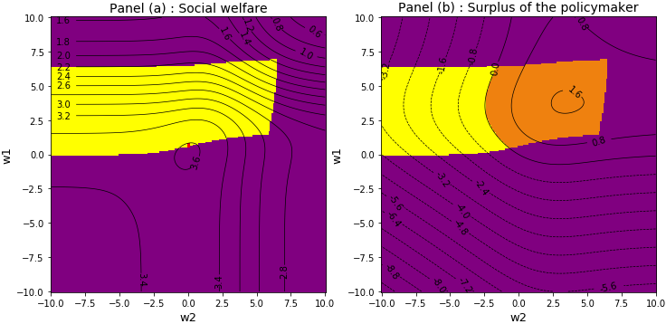
Figure 1. Panel (a) illustrates social welfare and Panel (b) shows PM’s surplus in the AE given ($w_{1}$, $w_{2}$). The vertical (horizontal) axis indicates the tax (or subsidy if negative) on region $z_{1}$ ($z_{2}$). The yellow + orange regions are the set of AE with regional constraints. The red point in (a) is the unique EAE. In (b), the orange region indicates BB-AE (AE with regional constraints in which the PM’s surplus is nonnegative) defined in Section 6.

Theorem 2.

Fix any $\Phi\in\mathbb{R}^{(|X|+1)\times(|Y|+1)}$. If $(\mu,(U,V,w))$ is an EAE, then $(U,V,\bar{w},\underline{w})$ is a solution to the optimization problem $($Theorem 2.$)$ and $\mu$ satisfies the market clearing condition, where $\bar{w}_{z}\coloneqq\max\{0,w_{z}\},\underline{w}_{z}\coloneqq-\min\{0,w_{z}\}$. Conversely, if $(U,V,\bar{w},\underline{w})$ is a solution to the optimization problem $($Theorem 2.$)$ and $\mu$ satisfies the market clearing condition, then $(\mu,(U,V,w))$ is an EAE.

$($D$)$ $\left|\hfill\@mathmargin\begin{minipage}{372.91345pt}\vspace{-0.25\baselineskip} \@@amsalign\underset{U,V,\bar{w}_{z},\underline{w}_{z}}{\text{minimize}}\quad&G(U)+H(V)+\sum_{z\in Z}\bar{o}_{z}\bar{w}_{z}-\sum_{z\in Z}\underline{o}_{z}\underline{w}_{z}\ \\ \text{subject to}\quad&U_{xy}+V_{xy}\geq\Phi_{xy}-\bar{w}_{z(y)}+\underline{w}_{z(y)}&\forall(x,y)\in T,\\ &U_{xy}\in\mathbb{R}\ \text{and}\ V_{xy}\in\mathbb{R}&\forall(x,y)\in T,\\ &\bar{w}_{z}\geq 0,\ \underline{w}_{z}\geq 0&\forall z\in Z. \vspace{-1.0\baselineskip}\end{minipage}\right.$

Corollary 1.

EAE always exists and is unique.

The dual problem $($Efficient Aggregate Equilibrium$)$ of $($Theorem 2.$)$ is

$($P$)$ $\left|\hfill\@mathmargin\begin{minipage}{372.91345pt}\vspace{-0.25\baselineskip} \@@amsalign&\underset{\mu}{\text{maximize}}&\quad&\sum_{(x,y)\in T}\mu_{xy}\Phi_{xy}+\mathcal{E}(\mu)&\\ &\text{subject to}&\quad&\sum_{y\in Y_{0}}\mu_{xy}=n_{x}&\forall x\in X,\\ &&\quad&\sum_{x\in X_{0}}\mu_{xy}=m_{y}&\forall y\in Y,\\ &&\quad&\underline{o}_{z}\leq\sum_{y\in z}\sum_{x\in X}\mu_{xy}\leq\bar{o}_{z}&\forall z\in Z,\\ &&\quad&\mu_{xy}\geq 0&\forall(x,y)\in T, \vspace{-1.0\baselineskip}\end{minipage}\right.$

where $\mathcal{E}(\mu)\coloneqq-G^{*}(\mu)-H^{*}(\mu)$, and $G^{*}$, $H^{*}$ are the Legendre-Fenchel transform of $G$, $H$:

(6) $$G^{*}(\mu) \coloneqq\begin{cases}\displaystyle{\sup_{U}\ \Bigl{\{}\sum_{x\in X}\sum_{y\in Y_{0}}\mu_{xy}U_{xy}-G(U)\Bigr{\}}}&\left(\forall x\in X,\sum_{y\in Y_{0}}\mu_{xy}\leq n_{x}\right)\\ \infty&\text{otherwise}\end{cases},$$

(7) $$H^{*}(\mu) \coloneqq\begin{cases}\displaystyle{\sup_{V}\ \Bigl{\{}\sum_{y\in Y}\sum_{x\in X_{0}}\mu_{xy}V_{xy}-H(V)\Bigr{\}}}&\left(\forall y\in Y,\ \sum_{x\in X_{0}}\mu_{xy}\leq m_{y}\right)\\ \infty&\text{otherwise}\end{cases}.$$

We can show that $($Efficient Aggregate Equilibrium$)$ corresponds to the social welfare maximization problem under the population and the regional constraints (See Appendix A.3 for more details). The optimal value of $($Efficient Aggregate Equilibrium$)$ coincides with that of $($Theorem 2.$)$ by strong duality. Thus, the taxation policy $(w_{z})_{z}$ obtained as a solution to these optimization problems maximizes social welfare. It is also worth mentioning that, while we potentially allow taxes to differ among different type pairs in the social welfare maximization problem $($Efficient Aggregate Equilibrium$)$, all pairs in the same region $z$ incur the same amount of tax $w_{z}$ under the welfare-maximizing taxation policy. The following corollary summarizes these observations.

Corollary 2.

EAE maximizes social welfare under regional constraints, whose taxation policy is not conditioned on the types of pairs but is dependent only on the region.

Proof.

See Appendix A.3. ∎

We give one possible scenario in which Theorem 2 and related results are useful to obtain the optimal taxation policy. Suppose that the data on the existing matching in the market without taxation policy is available. As mentioned in Section 3, then we can estimate $\Phi_{xy}$’s, assuming specific error term distributions, such as Gumbel distribution as in Example 1. The distributional assumption also determines the form of $G$ and $H$. Given $\Phi$, $G$, and $H$, we solve (D) to obtain taxation policy $w$, which is backed up from $\bar{w}$ and $\underline{w}$.

Example 0 (continues=exa:cont).

For each $w^{\prime}=(w^{\prime}_{1},w^{\prime}_{2})$ in Figure 1, there exists an AE $(\mu,(U,V,w’))$. The yellow area in Figure 1 represents the set of aggregate equilibria with regional constraint. We draw the contours of social welfare in Panel (a), and PM’s surplus (or deficit if negative and dotted lines) in Panel (b). As we see in Corollary 2, the red point $(w_{1},w_{2})=(0.583,0)$ in Panel (a) that tangents to the contour is the unique EAE. In Section 5, we will discuss budget balanced AE located in the orange area in Panel (b).

4.1. Proofs of Theorem 2 and Corollary 1

4.1.1. Proof of Theorem 1

First, we show two lemmas used in the main proof.

Lemma 0.

$G$ and $H$ are strictly increasing and strictly convex.

Proof.

$G$ is strictly increasing. Take any $U^{1},U^{2}\in\mathbb{R}^{N\times M}$ such that $U^{1}\geq U^{2}$ and $U^{1}\neq U^{2}$. Then $G(U^{1})\geq G(U^{2})$ by definition. In addition, note that $U^{1}_{xy}>U^{2}_{xy}$ holds for some $x\in X$ and $y\in Y$. Since $P_{x}$ has full support, we have

$$\text{Pr}_{\epsilon_{i}}(u_{i}=U^{1}_{xy}+\epsilon_{iy})\geq\text{Pr}_{\epsilon_{i}}(u_{i}=U^{2}_{xy}+\epsilon_{iy})>0.$$

Because $\mathbb{E}_{\epsilon_{i}}\left[u_{i}\mid u_{i}=U_{xy}+\epsilon_{iy}\right]$ is strictly increasing in $U_{xy}$, we have

$$\mathbb{E}_{\epsilon_{i}}\left[u_{i}\mid u_{i}=U^{1}_{xy}+\epsilon_{iy}\right] \cdot\text{Pr}_{\epsilon_{i}}(u_{i}=U^{1}_{xy}+\epsilon_{iy})$$

$$>\mathbb{E}_{\epsilon_{i}}\left[u_{i}\mid u_{i}=U^{2}_{xy}+\epsilon_{iy}\right]\cdot\text{Pr}_{\eta_{j}}(u_{i}=U^{2}_{xy}+\epsilon_{iy}),$$

and thus $G(U^{1})>G(U^{2})$ holds.

$G$ is strictly convex. Take any $U^{1},U^{2}\in\mathbb{R}^{N\times M}$ and $s\in[0,1]$. Since

$$sG(U^{1})+(1-s)G(U^{2}) =\sum_{x}n_{x}\mathbb{E}\left[\Bigl{(}\max_{y}\ s(U^{1}_{xy}+\epsilon_{iy})\Bigr{)}+\Bigl{(}\max_{y}\ (1-s)(U^{2}_{xy}+\epsilon_{iy})\Bigr{)}\right]$$

$$\geq\sum_{x}n_{x}\mathbb{E}\left[\max_{y}\ sU^{1}_{xy}+(1-s)U^{2}_{xy}+\epsilon_{iy}\right]$$

$$=G\Bigl{(}sU^{1}+(1-s)U^{2}\Bigr{)}$$

holds, $G$ is a convex function.

Now suppose $U^{1}\neq U^{2}$. Then $U^{1}_{xy}\neq U^{2}_{xy}$ holds for some $x\in X$, $y\in Y$. Without loss of generality, assume $U^{1}_{xy}>U^{2}_{xy}$. Since $P_{x}$ is full support,

$$\text{Pr}\Biggl{(}\Bigl{\{}\epsilon_{i}\mid U^{1}_{xy}+\epsilon_{iy}>\max_{y^{\prime}\neq y}U^{1}_{xy^{\prime}}+\epsilon_{iy^{\prime}}\hskip 10.00002pt\land\hskip 10.00002pt\max_{y^{\prime}\neq y}U^{2}_{xy^{\prime}}+\epsilon_{iy^{\prime}}>U^{2}_{xy}+\epsilon_{iy}\Bigr{\}}\Biggr{)}>0$$

holds. Therefore for any $s\in(0,1)$, we have

$$sG(U^{1})+(1-s)G(U^{2})>G\Bigl{(}sU^{1}+(1-s)U^{2}\Bigr{)},$$

which implies $G$ is strictly convex. Similarly, we can show $H$ is also strictly increasing and strictly convex. ∎

Lemma 0.

For each $x$ and $y$, if $\mu_{xy}>0$, then $U_{xy}+V_{xy}=\Phi_{xy}-w_{z(y)}$.

Proof.

Fix any $x$ and $y$. Suppose that $\mu_{xy}>0$. Then there exists $i$ and $j$ such that $x(i)=x$, $y(j)=y$, and $d_{ij}=1$. Suppose toward contradiction that $U_{xy}+V_{xy}>\Phi_{xy}-w_{z(y)}$. By the definition of $U_{xy}$ and $V_{xy}$, we have

$$u_{i}-\epsilon_{iy}+v_{j}-\eta_{xj}>\Phi_{xy}-w_{z(y)},$$

which implies that $u_{i}+v_{j}>\tilde{\Phi}_{ij}-w_{ij}$. A contradiction. ∎

Proof of Theorem 1.

Proof.

Let’s consider the necessary and sufficient conditions of the solution to $($Theorem 2.$)$. Let $(\lambda_{xy})_{x\in X,y\in Y}$, $(\bar{\lambda}_{z},\underline{\lambda}_{z})_{z\in Z}$ be lagrange multipliers, then the Lagrangean denoted by $\mathcal{L}$ is computed as follows;

$$\mathcal{L}=\ G(U)+H(V)+\sum_{z\in Z}\bar{o}_{z}\bar{w}_{z}-\sum_{z\in Z}\underline{o}_{z}\underline{w}_{z}$$

(8) $$+\sum_{x\in X,y\in Y}\lambda_{xy}\left(U_{xy}+V_{xy}-\Phi_{xy}+\bar{w}_{z(y)}-\underline{w}_{z(y)}\right)+\sum_{z\in Z}\bar{\lambda}_{z}\bar{w}_{z}+\sum_{z\in Z}\underline{\lambda}_{z}\underline{w}_{z}.$$

The KKT conditions are,

(9) $$\frac{\partial\mathcal{L}}{\partial U_{xy}}=\nabla_{xy}G(U)+\lambda_{xy}=0\quad\forall x\in X,y\in Y,$$

(10) $$\frac{\partial\mathcal{L}}{\partial V_{xy}}=\nabla_{xy}H(V)+\lambda_{xy}=0\quad\forall x\in X,y\in Y,$$

(11) $$\frac{\partial\mathcal{L}}{\partial\bar{w}_{z}}=\bar{o}_{z}+\sum_{y\in z}\sum_{x\in X}\lambda_{xy}+\bar{\lambda}_{z}=0\quad\forall z\in Z,$$

(12) $$\frac{\partial\mathcal{L}}{\partial\underline{w}_{z}}=-\underline{o}_{z}-\sum_{y\in z}\sum_{x\in X}\lambda_{xy}+\underline{\lambda}_{z}=0\quad\forall z\in Z,$$

(13) $$U_{xy}+V_{xy}-\Phi_{xy}+\bar{w}_{z(y)}-\underline{w}_{z(y)}\geq 0\quad\forall x\in X,y\in Y$$

(14) $$\lambda_{xy}\leq 0,\quad\lambda_{xy}\left(U_{xy}+V_{xy}-\Phi_{xy}+\bar{w}_{z(y)}-\underline{w}_{z(y)}\right)=0\quad\forall x\in X,y\in Y$$

(15) $$\bar{w}_{z}\geq 0,\ \bar{\lambda}_{z}\leq 0,\ \bar{\lambda}_{z}\bar{w}_{z}=0\quad\forall z\in Z$$

(16) $$\underline{w}_{z}\geq 0,\ \underline{\lambda}_{z}\leq 0,\ \underline{\lambda}_{z}\underline{w}_{z}=0\quad\forall z\in Z.$$

This satisfies the linearly independent constraint qualification, which implies these are the necessary conditions for the optimality.

From Lemma 4, the objective function of $($Theorem 2.$)$ is convex with respect to $(U,V,\bar{w},\underline{w})$. Because the constraints are linear in the parameters, KKT conditions are also sufficient conditions for the optimality.

EAE $\implies$ solution of $($Theorem 2.$)$$\colon$ Take any EAE $(\mu,(U,V,w))$ and define $\bar{w}_{z}=\max\{0,w_{z}\}$ and $\underline{w}_{z}=-\min\{0,w_{z}\}$ for all $z\in Z$.

Define $\lambda_{xy}=-\mu_{xy}$ for all $x\in X,y\in Y$. Then from condition 3 of EAE, the following holds;

$$-\lambda_{xy}=\mu_{xy}=\nabla_{xy}G(U)=\nabla_{xy}H(V),\quad\forall x\in X,y\in Y.$$

This implies that (9) and (10) are satisfied. Now $\mu_{xy}\geq 0$ implies $\lambda_{xy}\leq 0$. From condition 2 of EAE,

$$U_{xy}+V_{xy}-\Phi_{xy}+\bar{w}_{z(y)}-\underline{w}_{z(y)}=0.$$

This implies that (13)) and (14) are satisfied.

Next, when we define

$$\bar{\lambda}_{z} =\sum_{y\in z}\sum_{x\in X}\mu_{xy}-\bar{o}_{z}$$

$$\underline{\lambda}_{z} =\sum_{y\in z}\sum_{x\in X}-\mu_{xy}+\underline{o}_{z},$$

(11) and (12) are directly implied. Furthermore, by definition, $\bar{w}_{z},\underline{w}_{z}\geq 0$ for every $z\in Z$. And condition 4 of EAE implies that $\bar{\lambda}_{z}\leq 0$, $\underline{\lambda}_{z}\leq 0$. From condition 5 of EAE gives;

$$\bar{w}_{z}>0\implies w_{z}>0\implies\sum_{y\in z}\sum_{x\in X}\mu_{xy}=\bar{o}_{z}$$

$$\underline{w}_{z}>0\implies w_{z}<0\implies\sum_{y\in z}\sum_{x\in X}\mu_{xy}=\underline{o}_{z},$$

which implies that (15) and (16). So we are done with this part.

A solution of $($Theorem 2.$)$ $\implies$ EAE$\colon$ Take any $(U,V,\bar{w},\underline{w},\lambda)$ satisfying KKT conditions and define $\mu_{xy}=-\lambda_{xy}$ then (9) and (10) implies that $\mu_{xy}=\nabla_{xy}G(U)=\nabla_{xy}H(V)$ and so condition 3 is satisfied.

(11) and (15) implies;

$$\bar{\lambda}_{z}=-\sum_{y\in z}\sum_{x\in X}\lambda_{xy}-\bar{o}_{z}\leq 0\iff\sum_{y\in z}\sum_{x\in X}\mu_{xy}\leq\bar{o}_{z}.$$

Similarly, (12) and (16) implies;

$$\underline{\lambda}_{z}=\sum_{y\in z}\sum_{x\in X}\lambda_{xy}+\underline{o}_{z}\leq 0\iff\sum_{y\in z}\sum_{x\in X}\mu_{xy}\geq\underline{o}_{z}.$$

These says that condition 4 is satisfied.

Define $w_{z}=\bar{w}_{z}-\underline{w}_{z}$, then from (15) we get

$$w_{z}>0\implies\bar{w}_{z}>0\implies\bar{\lambda}_{z}=\sum_{y\in z}\sum_{x\in X}\mu_{xy}-\bar{o}_{z}=0.$$

Now from (16),

$$w_{z}<0\implies\underline{w}_{z}>0\implies\underline{\lambda}_{z}=-\sum_{y\in z}\sum_{x\in X}\mu_{xy}+\underline{o}_{z}=0.$$

Thus, we obtain condition 5 of EAE.

Next, from $\mu_{xy}=\nabla_{xy}G(U)=\nabla_{xy}H(V)$, we get

$$\sum_{y\in Y_{0}}\mu_{xy} =\sum_{y\in Y_{0}}\nabla_{xy}G(U)=n_{x}\sum_{y\in Y_{0}}\text{Pr}\Bigl{(}\{\epsilon_{iy}\mid u_{i}=U_{xy}+\epsilon_{iy}\}\Bigr{)}=n_{x},\quad\forall x\in X$$

$$\sum_{x\in X_{0}}\mu_{xy} =\sum_{x\in X_{0}}\nabla_{xy}H(V)=m_{y}\sum_{x\in X_{0}}\text{Pr}\Bigl{(}\{\eta_{xj}\mid v_{j}=V_{xy}+\eta_{xj}\}\Bigr{)}=m_{y},\quad\forall y\in Y.$$

This is equivalent to condition 1 of EAE.

Lastly, Assumption 4 assures us the following; for any $x\in X$, $y\in Y$,

$$-\lambda_{xy} =\nabla_{xy}G(U)=\text{Pr}\Bigl{(}\{\epsilon_{iy}\mid u_{i}=U_{xy}+\epsilon_{iy}\}\Bigr{)}>0$$

$$-\lambda_{xy} =\nabla_{xy}H(V)=\text{Pr}\Bigl{(}\{\eta_{xj}\mid v_{j}=V_{xy}+\eta_{xj}\}\Bigr{)}>0.$$

(14) implies

$$U_{xy}+V_{xy}=\Phi_{xy}-w_{z}(y),\quad\forall x\in X,y\in Y.$$

Hence, condition 2 of EAE is satisfied.

∎

4.1.2. Proof of Corollary 1

Existence$\colon$ First, observe that the feasible set of $($Theorem 2.$)$ is nonempty and convex. Then by the theorem of convex duality, $($Theorem 2.$)$ has a solution.

Uniqueness$\colon$ Fix any EAEs $(\mu,(U,V,w))$ and $(\mu^{\prime},(U^{\prime},V^{\prime},w^{\prime}))$. We want to show that $(\mu,(U,V,w))=(\mu^{\prime},(U^{\prime},V^{\prime},w^{\prime}))$.

Let $I(w)\coloneqq\sum_{z\in Z}\bar{o}_{z}\max\{0,w_{z}\}-\sum_{z\in Z}\underline{o}_{z}(-\min\{0,w_{z}\})$. Then, the objective function of $($Theorem 2.$)$ can be rewritten as

$$g(U,V,w)\coloneqq G(U)+H(V)+I(w).$$

Note that $I$ is convex, and hence $g$ is also convex.

Consider

$$(\mu^{\prime\prime},(U^{\prime\prime},V^{\prime\prime},w^{\prime\prime}))\coloneqq\frac{1}{2}(\mu,(U,V,w))+\frac{1}{2}(\mu^{\prime},(U^{\prime},V^{\prime},w^{\prime})).$$

Note that $(\mu^{\prime\prime},(U^{\prime\prime},V^{\prime\prime},w^{\prime\prime}))$ is feasible in $($Theorem 2.$)$. Since $G$ and $H$ are strictly convex and any EAE should be a solution to $($Theorem 2.$)$, we have $U=U^{\prime}=U^{\prime\prime}$ and $V=V^{\prime}=V^{\prime\prime}$; otherwise $g(U^{\prime\prime},V^{\prime\prime},w^{\prime\prime})<g(U,V,w)$ and this contradicts the optimality of $(U,V,w)$.

Suppose toward contradiction that $w\neq w^{\prime}$, or there exists $z_{0}$ such that $w_{z_{0}}\neq w^{\prime}_{z_{0}}$. First, note that since $U=U^{\prime}$ and $V=V^{\prime}$, we have $\mu=\mu^{\prime}$ by the market clearing condition.

Case (i): $\sum_{y\in{z_{0}}}\sum_{x}\mu_{xy}\in(\bar{o}_{z_{0}},\underline{o}_{z_{0}})$.

By the complementary slackness condition, we have $w_{z_{0}}=w^{\prime}_{z_{0}}$. A contradiction.

Case (ii): $\sum_{y\in{z_{0}}}\sum_{x}\mu_{xy}=\bar{o}_{z_{0}}$ ($>0$).

By the complementary slackness condition, we have $w_{z_{0}}\geq 0$ and $w^{\prime}_{z_{0}}\geq 0$. Since $w_{z_{0}}\neq w^{\prime}_{z_{0}}$, assume without loss of generality that $w_{z_{0}}>w^{\prime}_{z_{0}}\geq 0$. Let $\tilde{w}\coloneqq(w^{\prime\prime}_{z_{0}},w_{-z_{0}})$. Observe that $(U,V,\tilde{w})$ is feasible in $($Theorem 2.$)$.

Then, we have

(17) $$g(U,V,\tilde{w})-g(U,V,w) =\bar{o}_{z_{0}}(w^{\prime\prime}_{z_{0}}-w_{z_{0}})$$

(18) $$<0\quad(\because\ w^{\prime\prime}_{z_{0}}<w_{z_{0}}),$$

which contradicts the optimality of $(U,V,w)$.

Case (iii): $\sum_{y\in z}\sum_{x}\mu_{xy}=\underline{o}_{z_{0}}$.

If $\underline{o}_{z_{0}}>0$, we can show $w_{z_{0}}=w^{\prime}_{z_{0}}$ in a similar manner to case (ii).

Suppose that $\underline{o}_{z_{0}}=0$. Assume without loss of generality that $w_{z_{0}}>w^{\prime}_{z_{0}}\geq 0$. Let $\tilde{w}\coloneqq(0,w_{-z_{0}})$, and $\tilde{U}\coloneqq(U_{xy}-w_{z_{0}},U_{-(xy)})$. Observe that $(\tilde{U},V,\tilde{w})$ is feasible in $($Theorem 2.$)$. Since function $G$ is strictly increasing in $U_{xy}$ by Lemma 4, we have

$$g(\tilde{U},V,\tilde{w})<g(U,V,w),$$

which contradicts the optimality of $(U,V,w)$.

∎

5. Estimation of the Joint Surplus

So far, we have see how to compute the welfare-maximizing matching $\mu_{xy}$ given the known (already estimated) joint surplus $\Phi_{xy}$. This section, conversely, briefly explains how to estimate the joint surplus $\Phi_{xy}$ given matching patterns $\tilde{\mu}_{xy}$. We take the set of agent types $X$ and $Y$, their population $(n_{x})$ and $(m_{y})$. and regions $z(y)$ as given. Now suppose we have the data of

1. observed matching patterns $\tilde{\mu}=(\tilde{\mu}_{xy})_{x,y}$,

2. current tax levels $(w_{z})_{z}$, and

3. type-pair specific covariates $c=(c_{xy})_{x,y}$ (here $c_{xy}\in\mathbb{R}^{S}$ for some $S$).

The candidates of $c_{xy}$ are, for example, physical distances between the living area of type $x$ doctors and the office area of type $y$ hospitals, compatibility between doctors’ skills and job description, or characteristics that depend only on type $x$ or $y$ (such as doctor’s age or the average wage level around its office). It can simply be the vector of indicator functions of type pairs.

To estimate $\Phi_{xy}$, we first choose a parametric function $F_{\beta}$ that maps covariates $c_{xy}$ to joint surplus $\Phi_{xy}$, e.g. $F_{\beta}(c_{xy})=\beta^{\top}c_{xy}$ (linear regression). Then, we estimate $\beta$ by solving the nested optimization problem: we initialize $\beta=\beta^{0}$ and update $\beta$ in step $k$ as

1. Compute $\Phi_{xy}^{k}=F_{\beta^{k}}(c_{xy})$ for given $\beta^{k}$

2. Solve $($Estimation of the Joint Surplus$)$ and obtain the simulated matching $\mu^{k}$ using $\nabla_{xy}G=\nabla_{xy}H=\mu^{k}_{xy}$

3. Compute the error (distance) between the simulated matching $\mu^{k}$ and the observed matching $\tilde{\mu}$, $d(\mu^{k},\tilde{\mu})$

4. If $d(\mu^{k},\tilde{\mu})$ is small enough, finish the estimation. Them, the current $\Phi^{k}_{xy}=F_{\beta^{k}}(c_{xy})$ is the point estimate. Otherwise, update $\beta^{k}\to\beta^{k+1}$ so that $d$ becomes smaller and go back to Step 1.

$($D’$)$ $\left|\hfill\@mathmargin\begin{minipage}{372.91345pt}\vspace{-0.25\baselineskip} \@@amsalign\text{minimize}_{U,V}\ &G(U)+H(V)\\ \text{s.t.}\quad&U_{xy}+V_{xy}\geq\Phi_{xy}-w_{z(y)}\quad&\forall x\in X,y\in Y,\\ &U_{xy}\in{\mathbb{R}}\ \text{and}\ V_{xy}\in{\mathbb{R}}\quad&\forall x\in X,y\in Y. \vspace{-1.0\baselineskip}\end{minipage}\right.$

Note that $($Estimation of the Joint Surplus$)$ is a convex programming problem and the existence and the uniqueness of the solution are guaranteed like Corollary 1. Both the inner optimization problem (w.r.t. $\mu^{k}$) and the outer optimization problem (w.r.t. $\beta^{k}$) are solved by the standard optimization algorithm, e.g., Newton method.

The choice of the function $F_{\beta}$ and the distance $d$ is arbitrary. See (Galichon and Salanié, 2021) for the details. Here, we explain the maximum likelihood estimation (MLE). Let us adopt the Kullback-Leibler divergence of the multinomial distribution over the type pairs as $d$,

$$d(\tilde{\mu},\mu)\equiv\sum_{(x,y)\in T}(\tilde{\mu}_{xy}/|\tilde{\mu}|)\log\frac{(\tilde{\mu}_{xy}/|\tilde{\mu}|)}{(\mu_{xy}/|\mu|)},$$

where $|\mu|\equiv\sum_{(x,y)\in T}\mu_{xy}$. Given the matching data $\tilde{\mu}$, minimizing the KL-divergence is equivalent to maximizing the log-likelihood function

$$\log L(\beta)\propto\sum_{(x,y)\in T}\tilde{\mu}_{xy}\log\frac{\mu_{xy}}{|\mu|}.$$

Note that $\beta$ affects $\mu_{xy}$ through $\Phi_{xy}=F_{\beta}(c_{xy})$ and $($Estimation of the Joint Surplus$)$. By minimizing $d$ for the parameter $\beta$, we get the estimate of $\Phi_{xy}$ using the MLE.

6. Illustrative Experiment

This section compares EAE with other equilibrium concepts. To get intuition, we simulate a small tractable matching market of residencies with one urban region ($z_{1}$) and two rural regions ($z_{2},z_{3}$) in which all doctors prefer urban hospitals to rural hospitals on average. The policy challenge is to satisfy the minimum standards in the rural regions. We also conduct simulations with a larger number of types and regions in Appendix B.1 that describes the details of this section.

We assume there are 10 types of doctors and 6 types of hospitals, $\left|X\right|=10$ and $\left|Y\right|=6$. The population of each type is identical, $n_{x}=0.1$ for all $x\in X$ and $m_{y}=0.25$ for all $y\in Y$. There are three regions $z_{1}=z(y_{1})=z(y_{2})$, $z_{2}=z(y_{3})=z(y_{4})$, and $z_{3}=z(y_{5})=z(y_{6})$. Region $z_{1}$ is attractive for doctors (an urban area) while $z_{2}$ and $z_{3}$ are not (rural areas). All doctors are identical for each hospital on average. Specifically we set

$$\Phi_{xy}\coloneqq\begin{cases}2.0+\xi_{xy}&(x\in X,y\in z_{1})\\ 0.5+\xi_{xy}&(x\in X,y\in\{z_{2},z_{3}\})\end{cases},$$

where $\xi_{xy}$ are independent noise drawn from $N(0,1)$.

We assume there are lower bounds on rural areas, and no other constraints are imposed. We take the same lower bound $\underline{o}_{z}$ for the rural areas $z_{2}$ and $z_{3}$ ($\{\underline{o}_{z}\in\mathbb{R}\mid 0.1\leq\underline{o}_{z}\leq 0.4\}$) and set no lower bound on the urban area $\underline{o}_{z_{1}}=0$. We take an average of 30 simulations in Figure 2.

Let us compare EAE with three different aggregate equilibria (plus AE with no regional constraints (Unconstrained AE, U-AE) as a baseline). First, Upper-Bounded EAE (UB-EAE), instead of directly putting the lower bounds on rural regions, imposes the “loosest” upper bound on the urban ones so that a sufficient proportion of doctors moves to the urban regions under EAE. For example, if PM would like to fulfill the lower bounds $\underline{o}_{z_{1}}=\underline{o}_{z_{2}}=0.4$, UB-EAE instead sets an upper-bound with the smallest $\bar{o}_{z_{1}}$ satisfying $\sum_{x}\sum_{y\in z_{2}}\mu^{\text{UB-EAE}}_{xy}\geq 0.4$ and $\sum_{x}\sum_{y\in z_{3}}\mu^{\text{UB-EAE}}_{xy}\geq 0.4$. This technique is frequently used in non-transferable utility settings since feasible matchings need not exist with lower bounds (Fragiadakis et al., 2016; Kamada and Kojima, 2015). It is also illustrated by the second example in Section 1

Second, the Cap-Reduced AE (CR-AE) limits the maximum number of doctors matched in the urban area, instead of directly imposing the lower bounds on the rural areas, like UB-EAE. The difference is that PM artificially reduces the capacities of each hospital type in the urban area, instead of imposing an upper bound on the urban region. For example, instead of imposing the regional upper-bound $\bar{o}_{z_{1}}=0.4$ in UB-EAE, PM sets the artificial capacities $m_{y_{1}}=m_{y_{2}}=0.2$ of the urban hospital slots and computes AE without tax and subsidy. Although this policy inevitably causes inefficient matchings, it is easy to implement and a similar policy is frequently practiced, e.g., JRMP (Kamada and Kojima, 2015).

Finally, Budget-Balanced AE (BB-AE) requires PM to attain the budget-balanced, i.e.,
$\sum_{x,y}\mu_{xy}w_{z(y)}\geq 0$. BB-AE may not be unique as in Panel (b) of Figure 1. We concentrate on BB-AE which maximizes social welfare.

Interestingly, these equilibrium concepts are in an order w.r.t. social welfare for any problem instance.

Proposition 1.

For any instance, the levels of social welfare are in the following order:

$$\text{EAE}\geq\text{BB-AE}\geq\text{UB-EAE}\geq\text{CR-AE}.$$

The first inequality comes from the fact that EAE is welfare-maximizing as Corollary 2 states, the second one holds because UB-EAE imposes only taxes on urban areas so PM always makes a positive surplus, and the third one again follows from the same reason as the first one (under the alternative upper-bound constraints).

We show how we compute each equilibrium listed above in Appendix B.2.

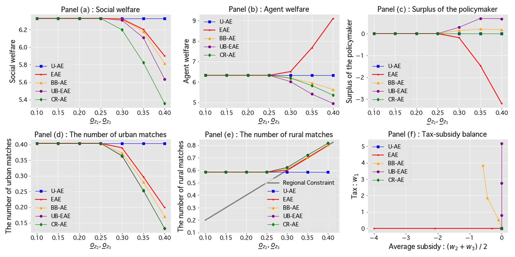
Figure 2. Panel (a)-(e): the horizontal axis is the lower bound constraints of rural regions ($\underline{o}_{z_{2}}=\underline{o}_{z_{3}}$), and the vertical axes indicate (a) the levels of the social welfare, (b) the agent welfare (the doctor welfare + the hospital welfare), (c) the PM surplus, (d) the number of matched doctors in the urban region $z_{1}$, and (e) in the rural regions $z_{2},z_{3}$ of each algorithm. The gray line in Panel (e) indicates the sum of the lower bounds of $z_{2},z_{3}$. Panel (f): the locus of the equilibrium tax and average subsidy of each method when $\underline{o}_{z_{2}}$ and $\underline{o}_{z_{3}}$ change. Note that U-AE and CR-EAE use neither tax nor subsidy, the blue, and the green lines stick to the origin.

Figure 2 summarizes how each equilibrium concept performs. Panel (a) illustrates how much social welfare each equilibrium achieves at each lower bound level to confirm Proposition 1. Panels (b) and (c) represent the agents’ (the doctors’ and the job slots’) welfare and the PM’s surplus, which reveals that in EAE, the social efficiency is achieved by relocating the surplus from the PM to the agents. Panels (d) and (e) show the number of doctors matched in the urban and the rural areas. We can see that EAE successfully keeps the number of doctors in $z_{1}$ as much as possible while tightly satisfying the rural lower bounds. Finally, Panel (f) depicts the locus of the tax and the average subsidy levels when $\underline{o}_{z}$ changes. It shows that EAE and UB-EAE are the complete opposites; EAE uses subsidies on the rural regions only while UB-EAE uses a tax on the urban regions only. Here BB-AE, balances a tax and subsidies so that it maximizes the social welfare in the range that the PM surplus remains nonnegative. When PM cannot make a deficit, the BB-AE is the second-best choice that is more desirable than UB-EAE or CR-EAE.

7. Summary and Discussion

This paper develops a framework to regulate matching markets with constraints. Extending the framework of (Galichon and Salanié, 2021), we propose a method to (1) estimate the utility functions of agents from currently available data on matching patterns, (2) predict outcomes under counterfactual taxation policies, and (3) design the welfare-maximizing taxation policy. Our results suggest that there may be a better way to satisfy regional constraints than current policies in practice.

Furthermore, our framework is valuable for policymakers who need to balance the tradeoff between the tightness of constraints and welfare loss. Although constraints are exogenously given in most papers in the literature on matching with constraints, our framework allows policymakers to estimate the cost of meeting different levels of regional quotas and make informed decisions.

We conclude our paper by pointing to a few possible future directions. First, our framework relies on a large market approximation, assuming that each type has sufficiently many agents. However, when PM has detailed individual data, she may use it to design a better policy without pooling agents with different types. It is worth considering how we can utilize such fine-grained data. Second, although our framework assumes transferable utilities, there is another thick strand of research on matching that assumes nontransferable utilities. Galichon et al. (2019) establish a general framework that includes both transferable and nontransferable utility matching as special cases. An extension of our framework to their setting is also promising. Lastly, it is worth evaluating the cost of large market assumption comparing its performance with exact methods.

Appendix A Omitted proofs

A.1. Proof of Lemma 2

Definition 0 (Total unimodularity).

Let $A$ be an integer matrix. $A$ is totally unimodular if any minor principal is either -1, 0, or 1.

Consider the following pair of linear programming problems:

(19) $$(\mathrm{P}^{\prime\prime})\left[\begin{matrix}\displaystyle{\max_{x\geq 0}}&\displaystyle{\sum_{i,j}\Phi_{ij}x_{ij}}\\[12.0pt] \mathrm{s.t.}&\sum_{j}x_{ij}\leq 1&(i\in I)\\ &\sum_{i}x_{ij}\leq 1&(j\in J)\\ &\sum_{j\in z}\sum_{i}x_{ij}\leq\bar{o}_{z}&(z\in Z)\\ &\sum_{j\in z}\sum_{i}x_{ij}\geq\underline{o}_{z}&(z\in Z)\end{matrix}\right.$$

(20) $$(\mathrm{D}^{\prime\prime})\left[\begin{matrix}\displaystyle{\max_{u,v,\bar{w},\underline{w}\geq 0}}&\displaystyle{\sum_{i}u_{i}+\sum_{j}v_{j}+\sum_{z\in Z}\bar{o}_{z}\bar{w}_{z}-\sum_{z\in Z_{L}}\underline{o}_{z}\underline{w}_{z}}\\[12.0pt] \mathrm{s.t.}&u_{i}+v_{j}\geq\Phi_{ij}-\bar{w}_{z(j)}+\underline{w}_{z(j)}&(i\in I,j\in J)\end{matrix}\right.$$

$(\mathrm{P}^{\prime\prime})$ is social welfare maximization problem with regional constraints, and $(\mathrm{D}^{\prime\prime})$ is its dual problem. First, we want to show the following lemma:

Lemma 0.

The matrix corresponds to the set of constraints of TU matching without regional constraints $(\mathrm{P}^{\prime\prime})$ is totally unimodular.

Our proof of Lemma 2 relies on the following fact about the total unimodularity.

Lemma 0 ((Ghouila-Houri, 1962)).

An $m\times n$ integer matrix $A$ is totally unimodular iff for each subset of rows $R\subseteq[m]$, there exists a partition $R_{1}$ and $R_{2}$ of $R$ such that

$$\forall k\in[n],\quad\sum_{i\in R_{1}}a_{ik}-\sum_{i\in R_{2}}a_{ik}\in\{-1,0,1\}$$

Proof of Proposition 2.

First, observe that the feasibility constraints (i.e., all the constraints except $x\geq 0$) of an instance of TU matching with regional constraints can be represented by $(|I|+|J|+2|Z|)\times(|I|\times|J|)$ matrix $A$ (See also Example 5) such that [itemize] @ Each row corresponds to either (1) agent $i\in I$, (2) agent $j\in J$, (3) an upper bound $\bar{o}_{z}$ for region $z\in Z$, or (4) a lower bound $\underline{o}_{z}$ for region $z\in Z$. @ Each column corresponds to an $(i,j)\in I\times J$ pair. @ The component of row $i\in I$ is 1 for column $(i,j^{\prime})$ for any $j^{\prime}\in J$; the component is 0 otherwise. @ The component of row $j\in J$ is 1 for column $(i^{\prime},j)$ for any $i^{\prime}\in I$; the component is 0 otherwise. @ Each region $z$ has two corresponding rows: one is for upper bound $\bar{z}$ and another one is for lower bound $\underline{z}$. @@ The component of row $\bar{z}$ is 1 for column $(i,j)$ such that $z(j)=z$; the component is 0 otherwise. @@ The component of row $\underline{z}$ is $-1$ for column $(i,j)$ such that $z(j)=z$; the component is 0 otherwise. We apply Lemma 3 to prove that $A$ is totally unimodular. Fix any subsets of rows $R$. Let $I_{R}\subseteq I$ be the rows corresponding to $i\in I$ contained in $R$. $J_{R}$, $\bar{Z}_{R}$, and $\underline{Z}_{R}$ are defined analogously.

We classify the rows in $R$ by a following algorithm:

1. Let $R_{1}\coloneqq\bar{Z}_{R}$ and $R_{2}\coloneqq\emptyset$.

2. For each $z\in\underline{Z}_{R}$, if $z\in\bar{Z}_{R}$, then $R_{1}\leftarrow R_{1}\cup\{z\}$; otherwise, $R_{2}\leftarrow R_{2}\cup\{z\}$.

3. Define a row vector $r(0)$ as

   $$r(0)\coloneqq\left(\sum_{i\in R_{1}}a_{ik}-\sum_{i\in R_{2}}a_{ik}\right)_{k}.$$

4. Let $J_{R}\coloneqq\{j(1),\dots,j(T_{J})\}$, $R_{1}(0)\coloneqq R_{1}$, and $R_{2}(0)\coloneqq R_{2}$. For each $t\in[T_{J}]$,

   1. If $r(0)_{i,j(t)}=1$ for some $i$, then $R_{1}(t)\coloneqq R_{1}(t-1)$ and $R_{2}(t)\coloneqq R_{2}(t-1)\cup\{j(t)\}$.

   2. Otherwise, $R_{1}(t)\coloneqq R_{1}(t-1)\cup\{j(t)\}$ and $R_{2}(t)\coloneqq R_{2}(t-1)$.

5. Let $R_{1}\coloneqq R_{1}(T_{J})$ and $R_{2}\coloneqq R_{2}(T_{J})\cup I_{R}$. Return $R_{1}$ and $R_{2}$.

We will show that why the algorithm above works. First, under the hierarchical regional constraints, each component of $r(0)$ is either 0 or 1. Next, let

$$r\coloneqq\left(\sum_{i\in R_{1}(T_{J})}a_{ik}-\sum_{i\in R_{2}(T_{J})}a_{ik}\right)_{k}.$$

Note that, under the regional constraints, if $z(j_{0})=z_{0}$ and $a_{j_{0},k}=1$, then $a_{\bar{z}_{0},k}=1$ and $a_{\underline{z}_{0},k}=-1$. Thus, by construction of Step 4, all the components of $r$ are either $0$ or $1$. Lastly, by construction, for any column $k$, $\sum_{i\in I_{R}}a_{ik}\in\{0,1\}$. Therefore, we have

$$\forall k\in[n],\quad\sum_{i\in R_{1}}a_{ik}-\sum_{i\in R_{2}}a_{ik}\in\{-1,0,1\}.$$

By Lemma 3, this implies that $A$ is totally unimodular. ∎

By the following well-known result, $(\mathrm{P}^{\prime\prime})$ has an integer optimal solution.

Lemma 0 ((Hoffman and Kruskal, 2010)).

$A$ is totally unimodular iff, for any $b\in\mathbb{Z}^{m}$, $P\coloneqq\{x\in\mathbb{R}^{n}\colon Ax\leq b,x\geq 0\}$ is an integral polyhedra, i.e., all the faces includes an integer vector. If $P$ is bounded, this is equivalent to that the components of all vertices of $P$ are integers.

Let $x$ be an integer optimal solution to $(\mathrm{P}^{\prime\prime})$ and let $(u,v,\bar{w},\underline{w})$ be a solution to (D”). By a similar argument as in the standatd TU matching model that characterizes an stable outcome as a solution to the social welfare maximization problem and its dual problem, we can show that $(x,(u,v),w)$ is an IE given $\Phi$, where $w_{z}\coloneqq\bar{w}_{z}\textbf{1}\{\bar{w}_{z}>0\}-\underline{w}_{z}\textbf{1}\{\underline{w}_{z}>0\}$. Note that $\bar{w}_{z}>0$ and $\underline{w}_{z}>0$ cannot happen simultaneously due to the complementary slackness condition.

Example 0 (TU matching with regional constraints).

Let $I\coloneqq\{i_{1},i_{2}\}$, $J\coloneqq\{j_{1},j_{2},j_{3}\}$, $Z\coloneqq\{z_{1},z_{2}\}$, $z(j_{1})=z(j_{2})=z_{1}$, and $z(j_{3})=z_{2}$. The set of constraints can be written as $A_{0}x\leq b$ by defining $A_{0}$, $x$, and $b$ as follows:

(22) $$A_{0} \coloneqq\hbox{}\vbox{\kern 0.86108pt\hbox{$\kern 0.0pt\kern 2.5pt\kern-5.0pt\left[\kern 0.0pt\kern-2.5pt\kern-5.55557pt\vbox{\kern-0.86108pt\vbox{\vbox{ \halign{\kern\arraycolsep\hfil\@arstrut$\kbcolstyle#$\hfil\kern\arraycolsep& \kern\arraycolsep\hfil$\@kbrowstyle#$\ifkbalignright\relax\else\hfil\fi\kern\arraycolsep&& \kern\arraycolsep\hfil$\@kbrowstyle#$\ifkbalignright\relax\else\hfil\fi\kern\arraycolsep\cr 5.0pt\hfil\@arstrut$\scriptstyle$\hfil\kern 5.0pt&5.0pt\hfil$\scriptstyle(i_{1},j_{1})$\hfil\kern 5.0pt&5.0pt\hfil$\scriptstyle(i_{1},j_{2})$\hfil\kern 5.0pt&5.0pt\hfil$\scriptstyle(i_{1},j_{3})$\hfil\kern 5.0pt&5.0pt\hfil$\scriptstyle(i_{2},j_{1})$\hfil\kern 5.0pt&5.0pt\hfil$\scriptstyle(i_{2},j_{2})$\hfil\kern 5.0pt&5.0pt\hfil$\scriptstyle(i_{2},j_{3})\\i_{1}$\hfil\kern 5.0pt&5.0pt\hfil$\scriptstyle 1$\hfil\kern 5.0pt&5.0pt\hfil$\scriptstyle 1$\hfil\kern 5.0pt&5.0pt\hfil$\scriptstyle 1$\hfil\kern 5.0pt&5.0pt\hfil$\scriptstyle 0$\hfil\kern 5.0pt&5.0pt\hfil$\scriptstyle 0$\hfil\kern 5.0pt&5.0pt\hfil$\scriptstyle 0\\i_{2}$\hfil\kern 5.0pt&5.0pt\hfil$\scriptstyle 0$\hfil\kern 5.0pt&5.0pt\hfil$\scriptstyle 0$\hfil\kern 5.0pt&5.0pt\hfil$\scriptstyle 0$\hfil\kern 5.0pt&5.0pt\hfil$\scriptstyle 1$\hfil\kern 5.0pt&5.0pt\hfil$\scriptstyle 1$\hfil\kern 5.0pt&5.0pt\hfil$\scriptstyle 1\\j_{1}$\hfil\kern 5.0pt&5.0pt\hfil$\scriptstyle 1$\hfil\kern 5.0pt&5.0pt\hfil$\scriptstyle 0$\hfil\kern 5.0pt&5.0pt\hfil$\scriptstyle 0$\hfil\kern 5.0pt&5.0pt\hfil$\scriptstyle 1$\hfil\kern 5.0pt&5.0pt\hfil$\scriptstyle 0$\hfil\kern 5.0pt&5.0pt\hfil$\scriptstyle 0\\j_{2}$\hfil\kern 5.0pt&5.0pt\hfil$\scriptstyle 0$\hfil\kern 5.0pt&5.0pt\hfil$\scriptstyle 1$\hfil\kern 5.0pt&5.0pt\hfil$\scriptstyle 0$\hfil\kern 5.0pt&5.0pt\hfil$\scriptstyle 0$\hfil\kern 5.0pt&5.0pt\hfil$\scriptstyle 1$\hfil\kern 5.0pt&5.0pt\hfil$\scriptstyle 0\\j_{3}$\hfil\kern 5.0pt&5.0pt\hfil$\scriptstyle 0$\hfil\kern 5.0pt&5.0pt\hfil$\scriptstyle 0$\hfil\kern 5.0pt&5.0pt\hfil$\scriptstyle 1$\hfil\kern 5.0pt&5.0pt\hfil$\scriptstyle 0$\hfil\kern 5.0pt&5.0pt\hfil$\scriptstyle 0$\hfil\kern 5.0pt&5.0pt\hfil$\scriptstyle 1\\\bar{z}_{1}$\hfil\kern 5.0pt&5.0pt\hfil$\scriptstyle 1$\hfil\kern 5.0pt&5.0pt\hfil$\scriptstyle 1$\hfil\kern 5.0pt&5.0pt\hfil$\scriptstyle 0$\hfil\kern 5.0pt&5.0pt\hfil$\scriptstyle 1$\hfil\kern 5.0pt&5.0pt\hfil$\scriptstyle 1$\hfil\kern 5.0pt&5.0pt\hfil$\scriptstyle 0\\\bar{z}_{2}$\hfil\kern 5.0pt&5.0pt\hfil$\scriptstyle 0$\hfil\kern 5.0pt&5.0pt\hfil$\scriptstyle 0$\hfil\kern 5.0pt&5.0pt\hfil$\scriptstyle 1$\hfil\kern 5.0pt&5.0pt\hfil$\scriptstyle 0$\hfil\kern 5.0pt&5.0pt\hfil$\scriptstyle 0$\hfil\kern 5.0pt&5.0pt\hfil$\scriptstyle 1\\\underline{z}_{1}$\hfil\kern 5.0pt&5.0pt\hfil$\scriptstyle-1$\hfil\kern 5.0pt&5.0pt\hfil$\scriptstyle-1$\hfil\kern 5.0pt&5.0pt\hfil$\scriptstyle 0$\hfil\kern 5.0pt&5.0pt\hfil$\scriptstyle-1$\hfil\kern 5.0pt&5.0pt\hfil$\scriptstyle 1$\hfil\kern 5.0pt&5.0pt\hfil$\scriptstyle 0\\\underline{z}_{2}$\hfil\kern 5.0pt&5.0pt\hfil$\scriptstyle 0$\hfil\kern 5.0pt&5.0pt\hfil$\scriptstyle 0$\hfil\kern 5.0pt&5.0pt\hfil$\scriptstyle-1$\hfil\kern 5.0pt&5.0pt\hfil$\scriptstyle 0$\hfil\kern 5.0pt&5.0pt\hfil$\scriptstyle 0$\hfil\kern 5.0pt&5.0pt\hfil$\scriptstyle-1\\(i_{1},j_{1})$\hfil\kern 5.0pt&5.0pt\hfil$\scriptstyle-1$\hfil\kern 5.0pt&5.0pt\hfil$\scriptstyle\\(i_{1},j_{2})$\hfil\kern 5.0pt&5.0pt\hfil$\scriptstyle$\hfil\kern 5.0pt&5.0pt\hfil$\scriptstyle-1\\(i_{1},j_{3})$\hfil\kern 5.0pt&5.0pt\hfil$\scriptstyle$\hfil\kern 5.0pt&5.0pt\hfil$\scriptstyle$\hfil\kern 5.0pt&5.0pt\hfil$\scriptstyle-1\\(i_{2},j_{1})$\hfil\kern 5.0pt&5.0pt\hfil$\scriptstyle$\hfil\kern 5.0pt&5.0pt\hfil$\scriptstyle$\hfil\kern 5.0pt&5.0pt\hfil$\scriptstyle$\hfil\kern 5.0pt&5.0pt\hfil$\scriptstyle-1\\(i_{2},j_{2})$\hfil\kern 5.0pt&5.0pt\hfil$\scriptstyle$\hfil\kern 5.0pt&5.0pt\hfil$\scriptstyle$\hfil\kern 5.0pt&5.0pt\hfil$\scriptstyle$\hfil\kern 5.0pt&5.0pt\hfil$\scriptstyle$\hfil\kern 5.0pt&5.0pt\hfil$\scriptstyle-1\\(i_{2},j_{3})$\hfil\kern 5.0pt&5.0pt\hfil$\scriptstyle$\hfil\kern 5.0pt&5.0pt\hfil$\scriptstyle$\hfil\kern 5.0pt&5.0pt\hfil$\scriptstyle$\hfil\kern 5.0pt&5.0pt\hfil$\scriptstyle$\hfil\kern 5.0pt&5.0pt\hfil$\scriptstyle$\hfil\kern 5.0pt&5.0pt\hfil$\scriptstyle-1$\hfil\kern 5.0pt\crcr}}}}\right]$}}\\x \coloneqq(x_{i_{1}j_{1}},x_{i_{1}j_{2}},x_{i_{1}j_{3}};x_{i_{2}j_{1}},x_{i_{2}j_{2}},x_{i_{2}j_{3}})^{\top}\\b \coloneqq(1,1,1,1,1,o_{z_{1}},o_{z_{2}},0,0,0,0,0,0)^{\top}$$

The last $|I|\times|J|$ rows corresponds to non-negativity constraints $x_{ij}\geq 0$. Note that $[B\ I]$ is totally unimodular if $B$ is totally unimodular. Thus, to show $A_{0}$ is totally unimodular, it suffices to show that

$$A\coloneqq\hbox{}\vbox{\kern 0.86108pt\hbox{$\kern 0.0pt\kern 2.5pt\kern-5.0pt\left[\kern 0.0pt\kern-2.5pt\kern-5.55557pt\vbox{\kern-0.86108pt\vbox{\vbox{ \halign{\kern\arraycolsep\hfil\@arstrut$\kbcolstyle#$\hfil\kern\arraycolsep& \kern\arraycolsep\hfil$\@kbrowstyle#$\ifkbalignright\relax\else\hfil\fi\kern\arraycolsep&& \kern\arraycolsep\hfil$\@kbrowstyle#$\ifkbalignright\relax\else\hfil\fi\kern\arraycolsep\cr 5.0pt\hfil\@arstrut$\scriptstyle$\hfil\kern 5.0pt&5.0pt\hfil$\scriptstyle(i_{1},j_{1})$\hfil\kern 5.0pt&5.0pt\hfil$\scriptstyle(i_{1},j_{2})$\hfil\kern 5.0pt&5.0pt\hfil$\scriptstyle(i_{1},j_{3})$\hfil\kern 5.0pt&5.0pt\hfil$\scriptstyle(i_{2},j_{1})$\hfil\kern 5.0pt&5.0pt\hfil$\scriptstyle(i_{2},j_{2})$\hfil\kern 5.0pt&5.0pt\hfil$\scriptstyle(i_{2},j_{3})\\i_{1}$\hfil\kern 5.0pt&5.0pt\hfil$\scriptstyle 1$\hfil\kern 5.0pt&5.0pt\hfil$\scriptstyle 1$\hfil\kern 5.0pt&5.0pt\hfil$\scriptstyle 1$\hfil\kern 5.0pt&5.0pt\hfil$\scriptstyle 0$\hfil\kern 5.0pt&5.0pt\hfil$\scriptstyle 0$\hfil\kern 5.0pt&5.0pt\hfil$\scriptstyle 0\\i_{2}$\hfil\kern 5.0pt&5.0pt\hfil$\scriptstyle 0$\hfil\kern 5.0pt&5.0pt\hfil$\scriptstyle 0$\hfil\kern 5.0pt&5.0pt\hfil$\scriptstyle 0$\hfil\kern 5.0pt&5.0pt\hfil$\scriptstyle 1$\hfil\kern 5.0pt&5.0pt\hfil$\scriptstyle 1$\hfil\kern 5.0pt&5.0pt\hfil$\scriptstyle 1\\j_{1}$\hfil\kern 5.0pt&5.0pt\hfil$\scriptstyle 1$\hfil\kern 5.0pt&5.0pt\hfil$\scriptstyle 0$\hfil\kern 5.0pt&5.0pt\hfil$\scriptstyle 0$\hfil\kern 5.0pt&5.0pt\hfil$\scriptstyle 1$\hfil\kern 5.0pt&5.0pt\hfil$\scriptstyle 0$\hfil\kern 5.0pt&5.0pt\hfil$\scriptstyle 0\\j_{2}$\hfil\kern 5.0pt&5.0pt\hfil$\scriptstyle 0$\hfil\kern 5.0pt&5.0pt\hfil$\scriptstyle 1$\hfil\kern 5.0pt&5.0pt\hfil$\scriptstyle 0$\hfil\kern 5.0pt&5.0pt\hfil$\scriptstyle 0$\hfil\kern 5.0pt&5.0pt\hfil$\scriptstyle 1$\hfil\kern 5.0pt&5.0pt\hfil$\scriptstyle 0\\j_{3}$\hfil\kern 5.0pt&5.0pt\hfil$\scriptstyle 0$\hfil\kern 5.0pt&5.0pt\hfil$\scriptstyle 0$\hfil\kern 5.0pt&5.0pt\hfil$\scriptstyle 1$\hfil\kern 5.0pt&5.0pt\hfil$\scriptstyle 0$\hfil\kern 5.0pt&5.0pt\hfil$\scriptstyle 0$\hfil\kern 5.0pt&5.0pt\hfil$\scriptstyle 1\\\bar{z}_{1}$\hfil\kern 5.0pt&5.0pt\hfil$\scriptstyle 1$\hfil\kern 5.0pt&5.0pt\hfil$\scriptstyle 1$\hfil\kern 5.0pt&5.0pt\hfil$\scriptstyle 0$\hfil\kern 5.0pt&5.0pt\hfil$\scriptstyle 1$\hfil\kern 5.0pt&5.0pt\hfil$\scriptstyle 1$\hfil\kern 5.0pt&5.0pt\hfil$\scriptstyle 0\\\bar{z}_{2}$\hfil\kern 5.0pt&5.0pt\hfil$\scriptstyle 0$\hfil\kern 5.0pt&5.0pt\hfil$\scriptstyle 0$\hfil\kern 5.0pt&5.0pt\hfil$\scriptstyle 1$\hfil\kern 5.0pt&5.0pt\hfil$\scriptstyle 0$\hfil\kern 5.0pt&5.0pt\hfil$\scriptstyle 0$\hfil\kern 5.0pt&5.0pt\hfil$\scriptstyle 1\\\underline{z}_{1}$\hfil\kern 5.0pt&5.0pt\hfil$\scriptstyle-1$\hfil\kern 5.0pt&5.0pt\hfil$\scriptstyle-1$\hfil\kern 5.0pt&5.0pt\hfil$\scriptstyle 0$\hfil\kern 5.0pt&5.0pt\hfil$\scriptstyle-1$\hfil\kern 5.0pt&5.0pt\hfil$\scriptstyle 1$\hfil\kern 5.0pt&5.0pt\hfil$\scriptstyle 0\\\underline{z}_{2}$\hfil\kern 5.0pt&5.0pt\hfil$\scriptstyle 0$\hfil\kern 5.0pt&5.0pt\hfil$\scriptstyle 0$\hfil\kern 5.0pt&5.0pt\hfil$\scriptstyle-1$\hfil\kern 5.0pt&5.0pt\hfil$\scriptstyle 0$\hfil\kern 5.0pt&5.0pt\hfil$\scriptstyle 0$\hfil\kern 5.0pt&5.0pt\hfil$\scriptstyle-1$\hfil\kern 5.0pt\crcr}}}}\right]$}}$$

is totally unimodular.

A.2. Proof of Lemma 2

First, we show the following lemma:

Lemma 0.

For any $(x,y)\in X\times Y$, we have $\Phi_{xy}-w_{z(y)}\leq U_{xy}+V_{xy}$.

Proof.

First, suppose that $i\in x$ is matched with hospital $j\in y$. We have

(23) $$u_{i} =\max_{j\in J}\{\tilde{\Phi}_{ij}-v_{j}\}$$

(24) $$=\max_{y\in Y}\max_{j\in Y}\{\Phi_{ij}-w_{z(y)}-v_{j}\}$$

(25) $$=\max_{y\in Y}\max_{j\in Y}\{\Phi_{xy}-w_{z(y)}+\epsilon_{iy}+\eta_{xj}-w_{z(y)}-v_{j}\}$$

(26) $$=\max_{y\in Y}\{\Phi_{xy}-w_{z(y)}+\epsilon_{iy}+\max_{j\in y}\{\eta_{xj}-v_{j}\}\}$$

(27) $$=\max_{y\in Y}\{\Phi_{xy}-w_{z(y)}+\epsilon_{iy}-V_{xy}\}$$

Thus, for any $i\in x$, we have

(28) $$u_{i} =\max\left\{\max_{y\in Y}\{\Phi_{xy}-w_{z(y)}+\epsilon_{iy}-V_{xy}\},\epsilon_{i,y_{0}}\right\}$$

(29) $$=\max_{y\in Y_{0}}\{\Phi_{xy}-w_{z(y)}+\epsilon_{iy}-V_{xy}\}.$$

Hence,

$$\Phi_{xy}-w_{z(y)}\leq u_{i}-\epsilon_{iy}+V_{xy}.$$

By taking the infimum over $i\in x$, we have

$$\Phi_{xy}-w_{z(y)}\leq U_{xy}+V_{xy},$$

for each $x\in X$ and $y\in Y$. ∎

Proof of Lemma 2.

For any type $x\in X$ doctor $i\in I$ with type $x$. By definition of $U_{xy}$, we have

(30) $$U_{xy} \leq u_{i}-\epsilon_{iy},\ \forall y\in Y_{0}$$

(31) $$\iff u_{i} \geq U_{xy}+\epsilon_{iy},\ \forall y\in Y_{0}$$

(32) $$\iff u_{i} \geq\max_{y\in Y_{0}}\{U_{xy}+\epsilon_{iy}\}.$$

Similarly, for any type $y\in Y$ and doctor $j\in J$ with type $y$, we have $v_{j}\geq\max_{x\in X_{0}}\{V_{xy}+\eta_{xj}\}$.

We want to claim that $u_{i}\leq\max_{y\in Y_{0}}\{U_{xy}+\epsilon_{iy}\}$. Suppose toward contradiction that there exists type $x\in X$ and doctor $i\in I$ with type $x$ such that

$$u_{i}>\max_{y\in Y_{0}}\{U_{xy}+\epsilon_{iy}\}.$$

First, consider the case where $i$ is matched with some hospital $j\in y$. Then

(33) $$\Phi_{ij}-w_{z(y)} =u_{i}+v_{j}$$

(34) $$>\Bigl{(}\max_{y^{\prime}\in Y_{0}}\ U_{xy^{\prime}}+\epsilon_{iy^{\prime}}\Bigr{)}+\Bigl{(}\max_{x^{\prime}\in X_{0}}\ V_{x^{\prime}y}+\eta_{x^{\prime}j}\Bigr{)}$$

(35) $$\geq U_{xy(j)}+\epsilon_{iy(j)}+V_{xy(j)}+\eta_{xj}$$

(36) $$\geq\Phi_{xy}-w_{z(y)}+\epsilon_{iy(j)}+\eta_{xj}\quad(\because\ \text{Lemma~{}\ref{lem:ineq_systematic_surplus}})$$

(37) $$=\Phi_{ij}-w_{z(y)}.$$

A contradiction. Next, consider the case where $i$ is unmatched. Then

(38) $$u_{i}=\Phi_{i,y_{0}}=\epsilon_{i,y_{0}}>\max_{y\in Y_{0}}\{U_{xy}+\epsilon_{iy}\}\geq\epsilon_{i,y_{0}}.$$

A contradiction. Therefore, we have $u_{i}\leq\max_{y\in Y_{0}}\{U_{xy}+\epsilon_{iy}\}$ and hence $u_{i}=\max_{y\in Y_{0}}\{U_{xy}+\epsilon_{iy}\}$.

$v_{j}=\max_{x\in X_{0}}\{V_{xy}+\eta_{xj}\}$ can be shown in a similar manner. It is worth noting that the proof of Lemma 2 does not use Assumptions 1, 2, and 4. ∎

A.3. Proof of Corollary 2

We will show that for any matching $\mu$ that satisfies the market clearing condition, the objective function of $($Efficient Aggregate Equilibrium$)$ represents the social welfare. First, we will show the following lemma:

Lemma 0.

For each $i$ and $j$, let

$$Y_{i}^{*}(U)\in\mathop{\rm arg~{}max}\limits_{y\in Y_{0}}\left\{U_{x(i),y}+\epsilon_{iy}\right\},\quad X_{j}^{*}(V)\in\mathop{\rm arg~{}max}\limits_{x\in X_{0}}\left\{V_{x,y(j)}+\eta_{xj}\right\}.$$

Given any feasible matching $\mu$ that satisfies the market clearing condition, the systematic utilities $U$ and $V$ are uniquely determined by

(39) $$\mu_{xy}=\nabla_{xy}G(U)=\nabla_{xy}H(V),\hskip 15.00002pt\forall(x,y)\in T$$

since $G$ and $H$ are strictly convex. Let us denote them by $U(\mu)$ and $V(\mu)$. Then, we have

$$\mathcal{E}(\mu)=\sum_{x\in X}n_{x}\mathop{\mathbb{E}}_{\epsilon_{i}\sim P_{x}}\left[\epsilon_{i,Y_{i}^{*}(U(\mu))}\right]+\sum_{y\in Y}m_{y}\mathop{\mathbb{E}}_{\eta_{j}\sim Q_{y}}\left[\eta_{X_{j}^{*}(V(\mu)),j}\right].$$

That is, $\mathcal{E}(\mu)$ is equal to the agents’ welfare that comes from the unobserved error terms.

Proof of Lemma 7.

First, we note that $U(\mu)$ and $V(\mu)$ attain the supremum on the RHS of (6) and (7) because (39) gives the first order conditions.

Let $\bar{\mu}_{xy}\coloneqq\mu_{xy}/n_{x}$, which is the proportion of type-$x$ agents matched with type-$y$ agents. For any $x\in X$ and any $U_{x}\coloneqq(U_{xy})_{y\in Y_{0}}$, define

(40) $$G_{x}(U_{x}) \coloneqq\mathop{\mathbb{E}}_{\epsilon_{i}\sim P_{x}}\left[\max_{y\in Y_{0}}\{U_{xy}+\epsilon_{iy}\}\right]$$

(41) $$=\sum_{y\in Y_{0}}U_{xy}\cdot\underbrace{\text{Pr}\left(y\in\mathop{\rm arg~{}max}\limits_{y^{\prime}\in Y_{0}}\{U_{x,y^{\prime}}+\epsilon_{iy^{\prime}}\}\right)}_{\text{choice probability of $y$}}+\mathop{\mathbb{E}}_{\epsilon_{i}\sim P_{x}}\left[\epsilon_{i,Y_{i}^{*}(U)}\right]$$

(42) $$=\sum_{y\in Y}\bar{\mu}_{xy}U_{xy}+\mathop{\mathbb{E}}_{\epsilon_{i}\sim P_{x}}\left[\epsilon_{i,Y_{i}^{*}(U)}\right].$$

Note that $U_{xy_{0}}=0$. By definition, we have $G(U)=\sum_{x\in X}n_{x}G_{x}(U_{x})$.

Let us consider the Legendre-Fenchel transform of $G_{x}$. That is

(43) $$G^{*}_{x}(\bar{\mu}_{x})\coloneqq\begin{cases}\displaystyle{\sup_{U_{x}}\left\{\sum_{y\in Y_{0}}\bar{\mu}_{xy}U_{xy}-G_{x}(U_{x})\right\}}&\left(\sum_{y\in Y}\bar{\mu}_{xy}\leq 1\right)\\[8.0pt] +\infty&(\text{otherwise})\end{cases},$$

and it follows that $G^{*}(\mu)=\sum_{x\in X}n_{x}G^{*}_{x}(\bar{\mu}_{x})$.

Then, we have

(44) $$-G^{*}(\mu) =\sum_{x\in X}n_{x}\left(-G^{*}_{x}(\bar{\mu}_{x})\right)$$

(45) $$=\sum_{x\in X}n_{x}\left[G_{x}(U_{x}(\mu))-\sum_{y}\bar{\mu}_{xy}U_{xy}(\mu)\right]$$

(46) $$=\sum_{x\in X}n_{x}\mathop{\mathbb{E}}_{\epsilon_{i}\sim P_{x}}\left[\epsilon_{i,Y_{i}^{*}(U(\mu))}\right].$$

The second equality follows from (43) and the definition of $U(\mu)$. The last equality follows from (42).

By a similar argument, we can show that

$$-H^{*}(\mu)=\sum_{y\in Y}m_{y}\mathop{\mathbb{E}}_{\eta_{j}\sim Q_{y}}\left[\eta_{X_{j}^{*}(V(\mu)),j}\right].$$

∎

Lemma 7 states that $\mathcal{E}(\mu)$ captures the social surplus unobserved by the policy maker, which is the summation of the error terms that contribute to the social surplus. Hence, the objective function of $($Efficient Aggregate Equilibrium$)$ indeed represents the social welfare in this economy. Because the objective function is concave and the constraints are linear, the optimal value of $($Efficient Aggregate Equilibrium$)$ coincides with that of $($Theorem 2.$)$. Therefore the EAE maximizes the social welfare under the regional constraints. Furthermore, the optimal tax scheme is obtained as the Lagrange multipliers for the regional constraints, they only depend on the binding region $z$. ∎

Appendix B Simulation Details

B.1. Simulate EAE in a Larger Market

Although EAE is relatively easy to compute by the convex programming $($Theorem 2.$)$, we measured how long it takes to compute. We use CVXPY solver on our M1 Max Macbook Pro (32GB memory, 2021 model). We simulate the markets with $|X|=10,20$ doctor types and $|Z|=5,10,\ldots,100$ regions. We assume each region has 10 types of hospitals.

The actual JRMP problem has 47 regions (all prefectures in Japan) and approximately 10000 residents in total each year. Here the market with 10 doctor types and 50 regions (500 hospital types) has 5000 doctor-hospital type pairs (two residents for each pair on average), which is enough large to imitate the actual market.

For each $|X|,|Y|,$ and $|Z|$, we define the populations as $n_{x}=1.0/|X|$ for $x\in X$ and $m_{y}=1.5/|Y|$ for $y\in Y$. We set the lower bounds for all regions; $\underline{o}_{z}=0.3/|Z|$. We do not impose upper bounds on the regions. We set

$$\Phi_{xy}\coloneqq 2.0+\xi_{xy}$$

for all $x\in X,y\in Y$, where $\xi_{xy}$ are independent noise drawn from $N(0,1)$. We measure the time to compute EAE 10 times for each $|X|$ and $|Z|$, and take the average of them. The result is illustrated in Figure 3. It is clear that EAE is fast enough to be used for estimation and counterfactual simulation.

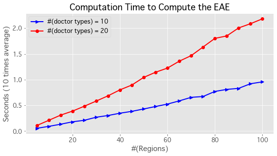
Figure 3. Average computation time (seconds) to compute EAE (an average of 10 trials). The number of doctor types are $|X|=10,20$ and the number of regions are $|Z|=5,10,15,\ldots,100$. Each region has 10 hospital types.

B.2. How to Compute Alternative Equilibria

B.2.1. Upper-bounded EAE (UB-EAE)

Given a lower bound for $\underline{o}_{z}=\underline{o}_{z_{2}}=\underline{o}_{z_{3}}$, we compute UB-EAE as follows; we set the 41 candidates of the upper bound for $z_{1}$ as $B=\{0.10,0.11,0.12,\ldots,0.50\}$, and

1. We take an upper bound for $z_{1}$, $\bar{o}_{z_{1}}$, from $B$ from the smallest.

2. Compute EAE under the regional constraint $\bar{o}_{z_{1}}$ (we do not impose other constraints; we set $\bar{o}_{z_{2}}=\bar{o}_{z_{3}}=\infty$ and $\underline{o}_{z}=0$ for all $z$). Let the EAE matching be $\mu$.

3. Check if the lower bounds for $z_{2}$ and $z_{3}$ are satisfied in EAE; check whether both $\sum_{x\in X}\sum_{y\in z_{2}}\mu_{xy}\geq\underline{o}_{z}$ and $\sum_{x\in X}\sum_{y\in z_{3}}\mu_{xy}\geq\underline{o}_{z}$ are satisfied.

   • If they are satisfied, then the current EAE is UB-EAE.

   • Otherwise, we take another candidate of the upper bound for $z_{1}$ from $B$ which is one step larger.

4. Repeat the above process until we find an UB-EAE.

In the current setting, we successfully find an UB-EAE for every lower bound.

B.2.2. Cap-reduced AE (CR-AE)

Given a lower bound for $\underline{o}_{z}=\underline{o}_{z_{2}}=\underline{o}_{z_{3}}$, we compute the unconstrained AE (U-AE) as follows; we set the 41 candidates of the artificial capacities of the urban hospitals $y_{1},y_{2}$ as $\hat{m}=\hat{m}_{y_{1}}=\hat{m}_{y_{2}}\in B=\{0.050,0.055,0.060,\ldots,0.25\}$, and

1. We take an artificial capacity $\hat{m}$ from $B$ from the smallest.

2. Compute U-AE under the artificial capacities $\hat{m}_{y_{1}}=\hat{m}_{y_{2}}=\hat{m}$ by $($Estimation of the Joint Surplus$)$ setting $w_{z}=0$ for all $z\in Z$ (note that we do not impose any regional constraints). Let the AE matching be $\mu$.

3. Check if the lower bounds for $z_{2}$ and $z_{3}$ are satisfied in AE; check whether both $\sum_{x\in X}\sum_{y\in z_{2}}\mu_{xy}\geq\underline{o}_{z}$ and $\sum_{x\in X}\sum_{y\in z_{3}}\mu_{xy}\geq\underline{o}_{z}$ are satisfied.

   • If they are satisfied, then the current AE is CR-AE.

   • Otherwise, we take another candidate of $\hat{m}$ from $B$ which is one step larger.

4. Repeat the above process until we find CR-AE.

In the current setting, we successfully find CR-AE for every lower bound.

B.2.3. Budget-balanced AE (BB-AE)

To compute BB-AE, we run the grid search; we set the candidates (grids) of taxes as

$$W=\Bigl{\{}(w_{1},w_{2},w_{3})\in\mathbb{R}^{3}\mid w_{1}\in\{0,0.5,1.0,\ldots,10.0\}\text{ and }w_{2},w_{3}\in\{-0.2,-0.19,-0.18,\ldots,0.00\}\Bigr{\}}.$$

For each $(w_{z_{1}},w_{z_{2}},w_{z_{3}})\in W$, we compute U-AE by $($Estimation of the Joint Surplus$)$ setting $(w_{z_{1}},w_{z_{2}},w_{z_{3}})$. Then for each lower bound for $\underline{o}_{z}=\underline{o}_{z_{2}}=\underline{o}_{z_{3}}$, we select the equilibrium that maximizes the social welfare among all BB-AE; it is computed as the solution to

$$\max_{\mu\in\hat{M}}\sum_{x\in X}\sum_{y\in Y}\mu_{xy}\left(\Phi_{xy}-w_{z(y)}\right)$$

where $\hat{M}$ is the set of all $\mu$ (U-AE for some $w\in W$) that satisfies

$$\sum_{x\in X}\sum_{y\in Y}\mu_{xy}w_{z(y)}\geq 0\quad\text{and}\quad\sum_{x\in X}\sum_{y\in z}\mu_{xy}\geq\underline{o}_{z}\text{ for each $z=z_{2},z_{3}$}.$$

References

• (1)
• Abdulkadiroğlu and Sönmez (2003) Atila Abdulkadiroğlu and Tayfun Sönmez. 2003. School Choice: A Mechanism Design Approach. American Economic Review 93, 3 (2003), 729–747.
• Agarwal and Somaini (2018) Nikhil Agarwal and Paulo Somaini. 2018. Demand analysis using strategic reports: An application to a school choice mechanism. Econometrica 86, 2 (2018), 391–444.
• Aguirregabiria and Mira (2010) Victor Aguirregabiria and Pedro Mira. 2010. Dynamic discrete choice structural models: A survey. Journal of Econometrics 156, 1 (2010), 38–67. https://doi.org/10.1016/j.jeconom.2009.09.007 Structural Models of Optimization Behavior in Labor, Aging, and Health.
• Azevedo and Leshno (2016) Eduardo M. Azevedo and Jacob D. Leshno. 2016. A Supply and Demand Framework for Two-Sided Matching Markets. Journal of Political Economy 124, 5 (2016), 1235–1268. https://doi.org/10.1086/687476 arXiv:https://doi.org/10.1086/687476
• Aziz et al. (2020) Haris Aziz, Anton Baychkov, and Péter Biró. 2020. Summer Internship Matching with Funding Constraints. In Proceedings of the 19th International Conference on Autonomous Agents and MultiAgent Systems. 97–104.
• Aziz et al. (2022) Haris Aziz, Péter Biró, and Makoto Yokoo. 2022. Matching Market Design with Constraints. In Proceedings of the AAAI Conference on Artificial Intelligence. 12308–12316.
• Aziz et al. (2019) Haris Aziz, Serge Gaspers, Zhaohong Sun, and Toby Walsh. 2019. From Matching with Diversity Constraints to Matching with Regional Quotas. In Proceedings of the 18th International Conference on Autonomous Agents and MultiAgent Systems. 377–385.
• Becker (1973) Gary S. Becker. 1973. A Theory of Marriage: Part I. Journal of Political Economy 81, 4 (1973), 813–846.
• Biró et al. (2010) Peter. Biró, Tamas. Fleiner, Robert.W. Irving, and David.F. Manlove. 2010. The College Admissions problem with lower and common quotas. Theoretical Computer Science 411, 34-36 (2010), 3136–3153.
• Bonhomme (2020) Stéphane Bonhomme. 2020. Econometric analysis of bipartite networks. Academic Press, 83–121. https://doi.org/10.1016/B978-0-12-811771-2.00011-0
• Choo and Siow (2006) Eugene Choo and Aloysius Siow. 2006. Estimating a marriage matching model with spillover effects. Demography 43, 3 (2006), 463–490. https://doi.org/10.1353/dem.2006.0023
• Demange (1982) Gabrielle Demange. 1982. Strategyproofness in the assignment market game. Laboratoire d’économétrie de l’École polytechnique.
• Ehlers et al. (2014) Lars Ehlers, Isa E. Hafalir, M. Bumin Yenmez, and Muhammed A. Yildirim. 2014. School Choice with Controlled Choice Constraints: Hard Bounds versus Soft Bounds. Journal of Economic Theory 153 (2014), 648–683.
• Fragiadakis et al. (2016) Daniel Fragiadakis, Atsushi Iwasaki, Peter Troyan, Suguru Ueda, and Makoto Yokoo. 2016. Strategyproof Matching with Minimum Quotas. ACM Transactions on Economics and Computation 4, Article 6 (2016). (an extended abstract appeared in AAMAS, pages 1327–1328, 2012).
• Gale and Shapley (1962) David Gale and Lloyd Stowell Shapley. 1962. College Admissions and the Stability of Marriage. The American Mathematical Monthly 69, 1 (1962), 9–15.
• Galichon et al. (2019) Alfred Galichon, Scott Duke Kominers, and Simon Weber. 2019. Costly Concessions: An Empirical Framework for Matching with Imperfectly Transferable Utility. Journal of Political Economy 127, 6 (2019), 2875–2925. https://doi.org/10.1086/702020 arXiv:https://doi.org/10.1086/702020
• Galichon and Salanié (2021) Alfred Galichon and Bernard Salanié. 2021. Cupid’s Invisible Hand: Social Surplus and Identification in Matching Models. Review of Economic Studies, forthcoming (2021).
• Ghouila-Houri (1962) Alain Ghouila-Houri. 1962. Caractérisation des matrices totalement unimodulaires. Comptes Redus Hebdomadaires des Séances de l’Académie des Sciences (Paris) 254 (1962), 1192–1194.
• Goto et al. (2016) Masahiro Goto, Atsushi Iwasaki, Yujiro Kawasaki, Ryoji Kurata, Yosuke Yasuda, and Makoto Yokoo. 2016. Strategyproof matching with regional minimum and maximum quotas. Artificial Intelligence 235 (2016), 40–57.
• Greinecker and Kah (2021) Michael Greinecker and Christopher Kah. 2021. Pairwise Stable Matching in Large Economies. Econometrica 89, 6 (2021), 2929–2974. https://doi.org/10.3982/ECTA16228 arXiv:https://onlinelibrary.wiley.com/doi/pdf/10.3982/ECTA16228
• Hafalir et al. (2013) Isa E. Hafalir, M. Bumin Yenmez, and Muhammed A. Yildirim. 2013. Effective affirmative action in school choice. Theoretical Economics 8, 2 (2013), 325–363.
• Hoffman and Kruskal (2010) Alan J Hoffman and Joseph B Kruskal. 2010. Integral boundary points of convex polyhedra. 50 Years of integer programming 1958–2008 (2010), 49.
• Jagadeesan et al. (2018) Ravi Jagadeesan, Scott Duke Kominers, and Ross Rheingans-Yoo. 2018. Strategy-proofness of worker-optimal matching with continuously transferable utility. Games and Economic Behavior 108 (2018), 287–294.
• Kamada and Kojima (2015) Yuichiro Kamada and Fuhito Kojima. 2015. Efficient Matching under Distributional Constraints: Theory and Applications. American Economic Review 105, 1 (2015), 67–99.
• Kawase and Iwasaki (2017) Yasushi Kawase and Atsushi Iwasaki. 2017. Near-Feasible Stable Matchings with Budget Constraints. In Proceedings of the 26th International Joint Conference on Artificial Intelligence. 242–248.
• Kawase and Iwasaki (2018) Yasushi Kawase and Atsushi Iwasaki. 2018. Approximately Stable Matchings with Budget Constraints. In Proceedings of the Thirty-Second AAAI Conference on Artificial Intelligence. Article 136, 1113–1120 pages.
• Kawase and Iwasaki (2020) Yasushi Kawase and Atsushi Iwasaki. 2020. Approximately Stable Matchings with General Constraints. In Proceedings of the 19th International Conference on Autonomous Agents and MultiAgent Systems. 602–610.
• Kelso and Crawford (1982) Alexander Kelso and Vincent Crawford. 1982. Job Matching, Coalition Formation, and Gross Substitutes. Econometrica 50, 6 (1982), 1483–1504.
• Kojima (2012) Fuhito Kojima. 2012. School choice: Impossibilities for affirmative action. Games and Economic Behavior 75, 2 (2012), 685–693.
• Kurata et al. (2017) Ryoji Kurata, Naoto Hamada, Atsushi Iwasaki, and Makoto Yokoo. 2017. Controlled School Choice with Soft Bounds and Overlapping Types. Journal of Artificial Intelligence Research 58 (2017), 153–184.
• McFadden (1980) Daniel McFadden. 1980. Econometric Models for Probabilistic Choice Among Products. The Journal of Business 53, 3 (1980), S13–S29.
• Nöldeke and Samuelson (2018) Georg Nöldeke and Larry Samuelson. 2018. The Implementation Duality. Econometrica 86, 4 (2018), 1283–1324. https://doi.org/10.3982/ECTA13307 arXiv:https://onlinelibrary.wiley.com/doi/pdf/10.3982/ECTA13307
• Roth and Sotomayor (1990) Alvin E. Roth and Marilda A. Oliveira Sotomayor. 1990. Two-Sided Matching: A Study in Game-Theoretic Modeling and Analysis (Econometric Society Monographs). Cambridge University Press.
• Shapley and Shubik (1971) Lloyd S Shapley and Martin Shubik. 1971. The assignment game I: The core. International Journal of game theory 1, 1 (1971), 111–130.