Study of Asymptotic Velocity in the Bondi-Hoyle Accretion Flows in the Domain of Kerr and 4-D Einstein-Gauss-Bonnet Gravities

Abstract

Understanding the physical structures of the accreated matter very close to the black hole in quasars and active galactic nucleus (AGNs) is an important milestone to constrain the activities occurring in their centers. In this paper, we numerically investigate the effects of the asymptotic velocities on the physical structures of the accretion disk around the Kerr and Einstein-Gauss-Bonnet (EGB) rapidly rotating black holes. The Bondi-Hoyle accretion is considered with a falling gas towards the black hole in upstream region of the computational domain. The shock cones are naturally produced in the downstream part of the flow around both black holes. It is found that the structure of the cones and the amount of the accreated matter depend on asymptotic velocity $V_{\infty}$ (Mach number) and the types of the gravities (Kerr or EGB). Increasing the Mach number of the inflowing matter in the supersonic region causes the shock opening angle and accretion rates getting smaller because of the rapidly falling gas towards the black hole. The EGB gravity leads to an increase in the shock opening angle of the shock cones while the mass accretion rates $\dot{M}$ are decreasing in EGB gravity with a Gauss-Bonnet (GB) coupling constant $\alpha$. It is also confirmed that accretion rates and drag forces are significantly altered in the EGB gravity. Our numerical simulation results could be used to identify the accreation mechanism and physical properties of the accretion disk and black hole in the observed $X-$ rays such as NGC $1313$ $X-1$ and $1313$ $X-2$ and MAXI $J1803-298$.

1 Introduction

The theory of the general relativity has already been confirmed by the large number of observational tests such as gravitational wave by LIGO (Abbott et al., 2016), the $M87*$ black hole shadow by Event Horizon Telescope (EHT) (Khodadi et al., 2020; Allahyari et al., 2020; Event Horizon Telescope Collaboration et al., 2019a, b, c), and the emitted electromagnetic spectrum from an accreation disk (Yuan & Narayan, 2014). In the strong gravitational region, the dynamics of the accretion disk close to the black hole uncovers the properties of the black hole and electromagnetic spectrum. It is certain that this region is influenced by the space-time curvature which depends on the black hole spin $a$ and GB coupling constant $\alpha$ in General Relativity (GR) and $4D$ Einstein-Gauss-Bonnet (EGB) gravity (Glavan & Lin, 2020).

The wind accretion onto the black hole potentially produces energetic outflows which can be used to define the black hole spin, mass and its shadow. The magnetically driven outflow onto the black hole is called Bondi-Hoyle-Lyttleton (BHL) accretion which is purely hydrodynamical (Hoyle & Lyttleton, 1939; Bondi & Hoyle, 1944; Edgar, 2004). The outflowing gas causes a formation of shock cone due to strong gravity in the vicinity of the black hole. For decades, BHL accretion was studied using the Newtonian and general relativistic hydrodynamics. Newtonian hydrodynamic was used to define the structure of the disk due to axisymmetric accretion flow for adiabatic gas (Hunt, 1971). $2D$ and $3D$ numerical simulations of the accretion disk had accomplished to reveal the dynamical structure of the disk, radiation mechanism, and properties of the compact objects (Foglizzo et al., 2005; Blondin, 2013; MacLeod & Ramirez-Ruiz, 2015; Ohsugi, 2018; Xu & Stone, 2019). Non-magnetized or magnetized relativistic BHL accretions around the non-rotating and rotating black holes have been simulated using either axial or spherical symmetries (Dönmez et al., 2011; Penner, 2011; Dönmez, 2012; Penner, 2012; Lora-Clavijo & Guzmán, 2013; Koyuncu & Dönmez, 2014; Lora-Clavijo et al., 2015; Gracia-Linares & Guzmán, 2015; Cruz-Osorio & Lora-Clavijo, 2016).

The modified theory of gravity received lots of attention when considering the solution of accretion disks. The accretion disk properties and their dynamical evolutions were studied in different modified gravity models such as the innermost circular orbits of spinning and massive particles (Zhang et al., 2020; Guo & Li, 2020), $f(R)$ gravity (Pun et al., 2008; Staykov et al., 2016), Einstein-Maxwell-dilation theory (Karimov et al., 2018; Heydari-Fard et al., 2020), scalar-tensor-vector gravity (Pérez et al., 2017), Einstein-scalar-Gauss-Bonnet gravity (Heydari-Fard & Sepangi, 2021), $4D$ $EGB$ gravity for non-rotating black hole (Liu et al., 2021), the observational constrain the $GB$ coupling constant $\alpha$ (Feng et al., 2020; Clifton et al., 2020), and for rotating black hole (Heydari-Fard et al., 2021). Heydari-Fard et al. (2021) had studied the thin accretion disk around rapidly rotating black hole. It is believed that the black hole would rotate with high rotation velocity due to the accreation effect.

The study of the dynamical evolution of the accretion disk around the non-rotating and the rotating black holes using different gravities would allow us to extract detailed information about the central objects, such as black hole shadow and physical properties as well as emission spectrum and temperature distribution of the accreation disk. The analytic solutions of the thin accreation disk around the $4D$ EGB gravity were studied in Gyulchev et al. (2021); Heydari-Fard et al. (2021); Guo et al. (2021); Liu et al. (2021); Malafarina et al. (2020) and referenced therein. They defined the electromagnetic properties of the disk and investigated the effects of GB coupling constant $\alpha$ and black hole rotation parameter $a$ on the properties of the accretion disk, the energy flux, and the electromagnetic spectrum. They also compared their results with the Kerr black hole solution. According to their results, the disk around the $4D$ EGB black hole for the positive value of $\alpha$ is more luminous and hotter than the one in General Relativity GR (Heydari-Fard et al., 2021). The numerical investigation of a BHL accretion in the $4D$ EGB extensively was studied in the vicinities of the non-rotating (Donmez, Orhan, 2021) and the rotating black holes (Donmez, 2022). They discussed the effect of GB coupling constant $\alpha$ on the shock cone structure created during the formation of the accretion disk.

The aim of this work is to model the accretion disk dynamics in the presence of the $4D$ EGB and Kerr strong gravities and to compare the shock cone properties from these two gravities. The matter will be accreated with a mechanism called a BHL accretion. The traveling black hole through a uniform medium causes the BHL accretion and the accreated matter towards the black hole from upstream side of computational domain forms a steady-state disk around the black hole. Since we are interested in the dynamics of the accretion disk, the shock cone, and accretion efficiency by using the different gravities, we explicitly study the effect of GB coupling constant $\alpha$ and the black hole rotation parameter $a$ on these dynamics.

In this paper, we model the non-magnetized BHL accretion onto the spinning black holes in $4D$ EGB and Kerr strong gravity regions to have a direct comparison between the two gravities. In section 2, brief descriptions of $4D$ EGB and Kerr rotating black hole space-time metric are presented along with the general relativistic hydrodynamical equations. The initial and boundary conditions used in numerical simulations are given in Section 3 in order to inject the gas from outer boundary of the computational domain. In Section 4, we present the results of our numerical simulations and discuss the consequences of two different gravities on the disk and shock cone dynamics. In Section 5, the astrophysical motivation of the numerical results is briefly discussed. The discussion and summary are presented in Section 6.

2 Rotating Black Hole Metric and General Relativistic Equations

The Bondi-Hoyle accretion of the perfect fluid in the case of rotating - Kerr and EGB black holes is studied by solving General Relativistic Hydrodynamical (GRH) equations in the curved background. The perfect fluid stress-energy-momentum tensor is

$$T^{ab}=\rho hu^{a}u^{b}+Pg^{ab},$$ (1)

$h$, $p$, $\rho$, $u^{a}$, and $g^{ab}$ are the specific enthalpy, the fluid pressure, the rest-mass density, the $4-$ velocity of the fluid, and the metric of the curved space-time, respectively. The indexes $a$, $b$ and $c$ go from $0$ to $3$. Two different coordinates are used to compare the dynamical evolution of the accretion disk around the rotating black hole. First, Kerr black hole in Boyer-Lindquist coordinate is (Dönmez et al., 2011)

$$ds^{2}=-\left(1-\frac{2Mr}{\sum^{2}}\right)dt^{2}-\frac{4Mra}{\sum^{2}}sin^{2}\theta dtd\phi+\frac{\sum^{2}}{\Delta_{1}}dr^{2}+\sum^{2}d\theta^{2}+\frac{A}{\sum^{2}}sin^{2}\theta d\phi^{2}$$ (2)

where $\Delta_{1}=r^{2}-2Mr+a^{2}$, and $A=(r^{2}+a^{2})^{2}-a^{2}\Delta sin^{2}\theta$. The lapse function and shift vector of the Kerr metric are $\tilde{\alpha}=(\sum^{2}\Delta_{1}/A)^{1/2}$ and $\beta^{i}=(0,0,-2Mar/A)$.

Second, the rotating black hole metric in $4D$ EGB gravity is (Donmez, 2022)

$$ds^{2} = -\frac{\Delta_{2}-a^{2}sin^{2}\theta}{\Sigma}dt^{2}+\frac{\Sigma}{\Delta_{2}}dr^{2}-2asin^{2}\theta\left(1-\frac{\Delta_{2}-a^{2}sin^{2}\theta}{\Sigma}\right)dtd\phi+\Sigma d\theta^{2}+$$ (3)

$$sin^{2}\theta\left[\Sigma+a^{2}sin^{2}\theta\left(2-\frac{\Delta_{2}-a^{2}sin^{2}\theta}{\Sigma}\right)\right]d\phi^{2},$$

where $\Sigma$ and $\Delta_{2}$ read as $\Sigma=r^{2}+a^{2}cos^{2}\theta$ and $\Delta_{2}=r^{2}+a^{2}+\frac{r^{4}}{2\alpha}\left(1-\sqrt{1+\frac{8\alpha M}{r^{3}}}\right)$. $a$, $\alpha$, and $M$ are spin parameter, Gauss-Bonnet coupling constant, and mass of the black hole, respectively. The horizons of the black holes were obtained by solving $\Delta_{1}=0$ and $\Delta_{2}=0$. The lapse function $\tilde{\alpha}$ and the shift vectors of the EGB metric are $\tilde{\alpha}=\sqrt{\frac{a^{2}(1-f(r))^{2}}{r^{2}+a^{2}(2-f(r))}+f(r)}$ and $\beta^{i}=(0,\frac{ar^{2}}{2\pi\alpha}\left(1-\sqrt{1+\frac{8\pi\alpha M}{r^{3}}}\right),0)$, respectively. $f(r)=1+\frac{r^{2}}{2\alpha}\left(1-\sqrt{1+\frac{8\alpha M}{r^{3}}}\right).$

In order to solve GRH equation numerically, we should write them in a conserved form (Dönmez, 2004):

$$\frac{\partial U}{\partial t}+\frac{\partial F^{r}}{\partial r}+\frac{\partial F^{\phi}}{\partial\phi}=S,$$ (4)

where $U$, $F^{r}$, $F^{\phi}$, and $S$ are the vectors of the conserved variables, of the fluxes along $r$ and $\phi$ directions, sources, respectively. The vectors of the conserved variables are written in terms of the primitive variables,

$$U=\begin{pmatrix}D\\ S_{j}\\ \tau\end{pmatrix}=\begin{pmatrix}\sqrt{\gamma}W\rho\\ \sqrt{\gamma}h\rho W^{2}v_{j}\\ \sqrt{\gamma}(h\rho W^{2}-P-W\rho)\end{pmatrix}$$ (5)

where $W=(1-\gamma_{a,b}v^{i}v^{j})^{1/2}$, $h=1+\epsilon+P/\rho$, $\epsilon$, and $v^{i}=u^{i}/W+\beta^{i}$ are the Lorentz factor, enthalpy, internal energy, and three-velocity of the fluid, respectively. The ideal gas equation of state is adopted to define the pressure of the fluid and three-metric $\gamma_{i,j}$ and its determinant $\gamma$ are computed using the four-metric of rotating black holes. Latin indices $i$ and $j$ go from $1$ to $3$. The flux and the source can be computed for any metric using the following equations,

$$\vec{F}^{i}=\begin{pmatrix}\tilde{\alpha}\left(v^{i}-\frac{1}{\tilde{\alpha}\beta^{i}}\right)D\\ \tilde{\alpha}\left(\left(v^{i}-\frac{1}{\tilde{\alpha}\beta^{i}}\right)S_{j}+\sqrt{\gamma}P\delta^{i}_{j}\right)\\ \tilde{\alpha}\left(\left(v^{i}-\frac{1}{\tilde{\alpha}\beta^{i}}\right)\tau+\sqrt{\gamma}Pv^{i}\right)\end{pmatrix}$$ (6)

and,

$$\vec{S}=\begin{pmatrix}0\\ \tilde{\alpha}\sqrt{\gamma}T^{ab}g_{bc}\Gamma^{c}_{aj}\\ \tilde{\alpha}\sqrt{\gamma}\left(T^{a0}\partial_{a}\tilde{\alpha}-\tilde{\alpha}T^{ab}\Gamma^{0}_{ab}\right)\end{pmatrix}$$ (7)

where $\Gamma^{c}_{ab}$ is the Christoffel symbol.

3 Initial and Boundary Conditions

To study the Bondi-Hoyle accretion onto the rotating Gauss-Bonnet black hole and compare it with the Kerr black hole, GRH equations are solved on the equatorial plane using the code explained in Dönmez (2004, 2012); Donmez (2006). The pressure of the accreated matter is handled by using the standard $\Gamma$ law equation of state for a perfect fluid, $P=(\Gamma-1)\rho\epsilon$ with $\Gamma=4/3$. We adjusted the initial density and pressure profiles to ensure that the speed of sound equals to $C_{\infty}=0.1$ at the upstream region of the computational domain. After setting the density to be a constant value $(i.e.\;\rho=1)$, the pressure is computed from the perfect fluid equation of state, then we perform the numerical simulation on the equatorial plane using different values of asymptotic velocities. The initial velocities of the falling matter are given in terms of an asymptotic velocity $V_{\infty}$ at the upstream region and they are defined by the following equations, (Dönmez et al., 2011; Dönmez, 2012; Donmez, Orhan, 2021)

$$v^{r} = \sqrt{\gamma^{rr}}V_{\infty}cos(\phi)$$

$$v^{\phi} = -\sqrt{\gamma^{\phi\phi}}V_{\infty}sin(\phi).$$ (8)

Using various values of $V_{\infty}$ allows us to investigate different regimes around the black hole and therefore consider subsonic and supersonic accretion. The matter injected in the upstream region falls into a region assumed empty with $V^{r}=0$, $V^{\phi}=0$, and $\rho=10^{-4}$ in the beginning of the simulation $(i.e.\;t=0)$. The description of the initial models around the rotating black holes, Kerr and Gauss-Bonnet, with a spin $a/M=0.97$ is reported in Table 1.

Table 1: Adopted initial model used in the numerical simulation for Kerr and Gauss-Bonnet black holes. $type$ is the black hole types used in numerical simulations. $\alpha$ is Gauss-Bonnet coupling constant, $V_{\infty}$ is the asymptotic velocity of the matter falling towards the black hole at infinity, $M_{\infty}=V_{\infty}/C_{\infty}$ is the asymptotic Mach number at infinity.

$type$	$\alpha(M^{2})$	$V_{\infty}$	$M_{\infty}$
	$-$	$0.1$	$1$
	$-$	$0.2$	$2$
$Kerr$	$-$	$0.3$	$3$
	$-$	$0.4$	$4$
	$-$	$0.5$	$5$
	$-$	$0.6$	$6$
	$0.0064$	$0.1$	$1$
	$0.0064$	$0.2$	$2$
$Gauss-Bonnet$	$0.0064$	$0.3$	$3$
	$0.0064$	$0.4$	$4$
	$0.0064$	$0.5$	$5$
	$0.0064$	$0.6$	$6$
	$-0.1088$	$0.1$	$1$
	$-0.1088$	$0.2$	$2$
$Gauss-Bonnet$	$-0.1088$	$0.3$	$3$
	$-0.1088$	$0.4$	$4$
	$-0.1088$	$0.5$	$5$
	$-0.1088$	$0.6$	$6$
	$-0.5912$	$0.01$	$0.1$
	$-0.5912$	$0.05$	$0.5$
	$-0.5912$	$0.1$	$1$
	$-0.5912$	$0.2$	$2$
$Gauss-Bonnet$	$-0.5912$	$0.3$	$3$
	$-0.5912$	$0.4$	$4$
	$-0.5912$	$0.5$	$5$
	$-0.5912$	$0.6$	$6$

The uniformly spaced zones are used in radial and angular directions $N_{r}=1024$ and $N_{\phi}=256$. The inner and outer boundaries of the computational domain in the radial direction are located at $r_{min}=2.3M$ and $r_{max}=100M$, respectively, and $\phi_{min}=0$ and $\phi_{max}=2\pi$ in the angular direction. It is confirmed that the qualitative results of the numerical solutions (i.e. appearance of QPOs and instabilities, the shock location, the behavior of the accretion rates) are not sensitive to the grid resolution.

The corrected treatment of the boundary is important to avoid unphysical solutions in the numerical simulations. At the inner radial boundary, we implement outflow boundary condition to let the gas falling into a black hole by a simple zeroth-order extrapolation. On the other hand, we have to distinguish the downstream $-\pi/2<\phi<\pi/2$ and the upstream region $\pi/2\leq\phi\leq 3\pi/2$. While we adopt the outflow boundary condition in the downstream region, the gas is injected continuously with the initial velocities given in Eq.8 in the upstream region. The periodic boundary is used along the $\phi$-direction.

4 The Numerical Simulation of the accretion onto 4D EGB Rotating and Kerr Black Holes

In order to reveal the effect of asymptotic Mach number $(M_{\infty})$ on the dynamics of BHL accreation, we need to describe the morphology of the disk using the initial model $\alpha=-0.5912$ for GB coupling constant in Table1. For an adjusted value of speed of sound $C_{\infty}=0.1$, there is a critical value of asymptotic Mach number which equals to unity, above and bellow which shock cones form in the downstream side of computational domain when the matter is accreated upstream side seen in Fig.1. We plot the logarithm of the rest-mass density and linearly spaced isocontours on the equatorial plane. The disk is initially filled with matter falling from upstream side of the region. It is indicated in Fig.1 that, for $M_{\infty}=1$, the shock opening angle is getting wider and the shock cone is forced to convert into a bow shock due to ram pressure, gas pressure and strong gravity. This model indicates that asymptotic Mach number plays a critical role in the creation of shock cone and its opening angle and it prevents the shock cone created in the upstream region of the computational domain. Due to the strong gravity, the shock cone becomes attached to the black hole which produces accretion rate higher in the strong gravitational region (Ruffert, 1994; Ruffert & Arnett, 1994). As clearly shown in Fig.1, higher the asymptotic Mach number creates a shock cone with a smaller shock opening angle. The cone with a standing shock converts kinetic energy into thermal energy by falling material toward the rapidly rotating black hole in $4D$ EGB gravity. In addition, the shape of a shock cone very close to the black hole strongly depends on the black hole spin. As seen in Fig.1, due to the rapidly rotating black hole $a=0.97$, induced frame dragging produces a warping in space-time as well as the shock cone connected to the black hole horizon.

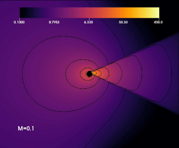
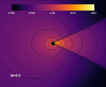
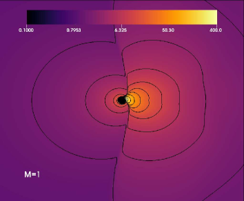
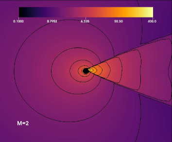
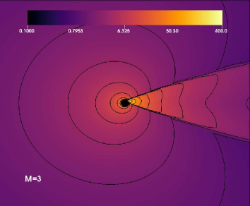
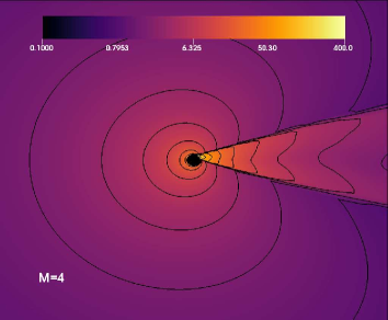
Figure 1: BHL accreation from the subsonic flow ($M_{\infty}<1$), sonic flow ($M_{\infty}=1$), and supersonic flow ($M_{\infty}>1$). The logarithm of the rest-mass density for asymptotic Mach number $(M_{\infty})$ given in left bottom corner of each plot for model $\alpha=-0.5912$ on the equatorial plane ($r-\phi$). The opening angle of the shock cones decreases with the increasing of $M_{\infty}$ in the supersonic flow.

In Fig.2, the behavior of the shock cone width with Kerr and $4D$ EGB gravities for different values of asymptotic velocities $V_{\infty}$ and the comparison of the results from these two gravities are given around the rapidly rotating black hole $a=0.97$. It is obvious that $4D$ EGB gravity has a big influence on the physical properties of the matter around the black hole and this is also confirmed by Liu et al. (2021). The effect of the asymptotic velocity on the cone width is clearly seen for the BHL accreation around the $4D$ EGB gravity as well as the Kerr gravity. Although the comparison of shock opening angle for different values of $V_{\infty}$ shows the same trend in all models, the shock opening angle is smaller around the Kerr black hole. It is seen that, for the $4D$ EGB gravity, the shock opening angle for any value of GB coupling constant $\alpha$ (positive or negative) is greater than the case in Kerr black hole and as the value of $\alpha$ in negative direction increases, the deviation from the Kerr geometry increases too. As it is observed in Fig.1, the shock cone opening angle decreases with increasing of asymptotic velocity or Mach number seen in Fig.2.

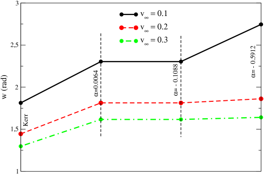
Figure 2: Cone width in terms of asymptotic velocity for Kerr and EGB black holes.

To reveal the dynamical properties of disk structure and the shock cone location, in Fig.3, we show the rest-mass density plot at a fixed radial distance $r=4.78M$ for asymptotic velocity $V_{\infty}=0.1$ at the final time of the evolution $t=30000M$. As seen in Fig.5, the shock cone under these conditions formed and reached the steady state around $t=13000M$. As mentioned earlier, the critical value of asymptotic velocity (Mach number) is $V_{\infty}=0.1$ $(M_{\infty}=1)$. The critical value of Mach number causes a creation of strongly oscillating accretion disk in our models. The effect of the GB coupling constant $\alpha$ on the shock cone density at final time is slightly varying as seen in Fig.3. Kerr black hole case is also plotted on the same figure to compare with the corresponding results and find that the rest-mass density is slightly higher in Kerr case. On the other hand, the angular position of the shock location is shifted for different values of $\alpha$. The inspection of different curves displayed in Fig.3 shows slight differences in the flow morphology.

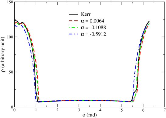
Figure 3: The densities of shock cones to showing the location of discontinuities are plotted as a function of angular distance at fixed $r=4.78M$ for asymptotic velocity $V_{\infty}=0.1$.

To complete the overall picture of shock cone structure and morphology of the accretion disk, Fig.4 shows the one-dimensional profile of the rest-mass density at the final time of simulation at different locations along the radial shells for asymptotic velocity $V_{\infty}=0.1$ and GB coupling constant $\alpha=-0.5912$. Clearly, the strong shock waves are created at the border of the shock cone. The angular location of the shock cone is slightly changed and shifted with the radial distance $r$. As it is expected, the rest-mass density gradually decreases with increasing $r$. The created shock cone would contribute to the radiation properties of the disk-black hole system. The shock cone is a very important physical mechanism which converts gravitational energy to the radiation energy and tapes and excites the oscillation modes. The shock cone could also be used to explain the erratic spin behavior variety found in different $X-$ray observations (Gergely & Biermann, 2009; Mould, 2021).

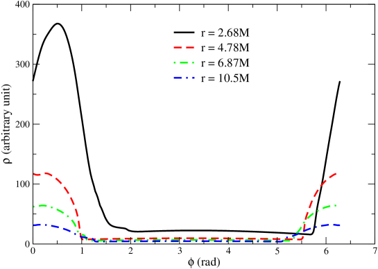
Figure 4: The shock cone locations as a function of angular distance for asymptotic velocity $V_{\infty}=0.1M$ and Gauss-Bonnet coupling constant $\alpha=-0.5912$ at different $r$.

As seen in the above discussion, the shock cone is the one of the consequences of the BHL accretion around the black bole in different gravities. The steady-state shock cone forms due to the effect of gravitation and pressure forces on the equatorial plane. Computing the mass accretion rate gives us more completed picture about the dynamics and instability of the shock cone around the rotating black hole. In Fig.5, the time evolution of the mass accretion rate for all the models for asymptotic velocity $V_{\infty}=0.1$ is shown. The different colors and line styles are used to separate the different models. The accretion rate is calculated using the following expression

$$\frac{dM}{dt}=-\int_{0}^{2\pi}\tilde{\alpha}\sqrt{\gamma}\rho u^{r}d\phi.$$ (9)

Although the accretion would lead to an increase in the mass of the black hole during the evolution, it is assumed that the black hole mass is constant during the whole simulation. As seen in Fig.5, the shock cone reaches steady-state around $t=13000M$ in all models and the accreation rate is the highest in Kerr gravity than EGB gravity for any value of GB coupling constant. After the cone reaches steady-state, it oscillates around a certain value. The oscillation amplitude is slightly diminished in the case of $\alpha=-0.5912$ for a fixed value of the black hole rotation parameter $a=0.97$. The greater the oscillation amplitude inside the shock cone would lead to a varying $X-$ ray in observed astrophysical phenomena.

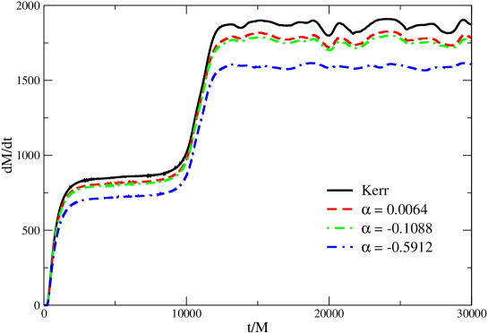
Figure 5: Mass accretion rate for asymptotic velocity $V_{\infty}=0.1$.

In order to extract more information about the possibility of the oscillation of the shock cone depending on asymptotic velocity and GB coupling constant we plot Fig.6. Once the shock cone reaches the steady state, we do not observe any oscillation for all values of $V_{\infty}$ except $V_{\infty}=0.1$. It is also noted that the quantitative value of accretion rate has the highest value in Kerr gravity. The accretion rate is getting smaller with increasing the negative value of GB coupling constant. Another trend, which is clearly seen in Fig.6, is that the steady state is fully developed around $t=2500M$ for any value of $V_{\infty}$ except $V_{\infty}=0.1$. The stability is first developed around $t=2500M$ for $V_{\infty}=0.1$ and later the shock cone goes into another unstable region around $t=10000M$. Finally, the steady state is attained around $t=12500M$. In the steady state, the shock cone formed in vicinity of the black hole on the equatorial plane is supposed to be in thermodynamical equilibrium. On the other hand, it is found that the accretion efficiency depends on GB coupling constant $\alpha$. The black hole with negative $\alpha$ can provide less efficient accreation mechanism which causes the transformation of the gravitational energy into the electromagnetic energy (Liu et al., 2021).

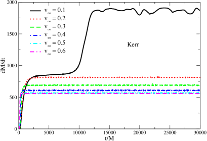
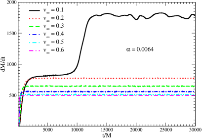
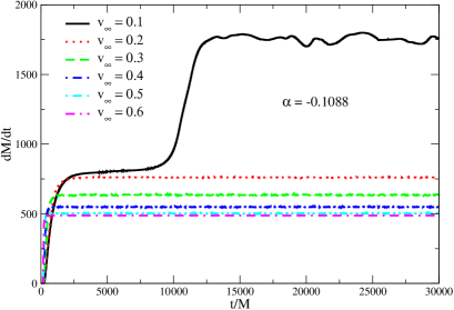
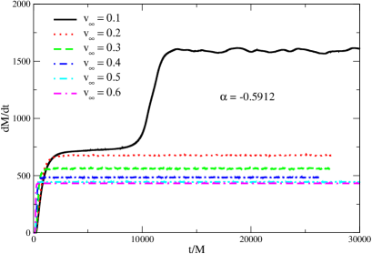
Figure 6: Mass accretion rates versus times for Kerr and EGB black holes.

Prediction of the accretion rates from the numerical simulation around the rotating black holes could be used to define the properties of the black hole as well as $X-$ ray mechanism. In Fig.7, we plot the behavior of the accretion rate with an asymptotic velocity at different locations along the radial distance on the disk. As seen in the Fig.7, the accretion rates exponentially decrease around the sonic point which occurs at $V_{\infty}=0.1$ . The reason of this decrease is due to the gravitational force and the pressure forces that they cannot balance each other and it causes a sudden change in the flow morphology when the velocity goes in the direction of subsonic or supersonic region. The gravitational force is dominant in the subsonic region while the gas pressure is dominant in the supersonic region, especially far away from the strong gravitational region.

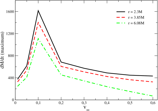
Figure 7: The maximum mass accretion rate shown as a function of $V_{\infty}$ at different radial shells for model $\alpha=-0.5912$.

The radial velocity profile is an important indicator to extract the violent features of the accreation mechanism and shock cone created around the black hole in different gravities. The kinetic energy of the violent motion depicts the thermal efficiency of the system. The color and counter plots of the radial velocity profile of the shock cone in strong gravitational region are shown in Fig.8 for Kerr and EGB gravities. The shock cone structure and radial velocity can be seen in the figure. While the matter is falling toward the black hole in one side of the shock cone location (positive velocity) it moves away from the other location (negative velocity). But the matter inside the shock cone oscillates in steady state. The dynamically stable flow seen in Fig.8 produces a continuum mechanism for creation of $X-$ ray around the rapidly rotating black holes. It is also shown that the behavior of the counter lines inside the shock cone around the Kerr black hole is slightly different than the ones in EGB gravity. In addition, there is no noticeable effect observed for the different values of GB coupling constant $\alpha$ in the strong gravitational region.

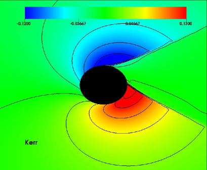
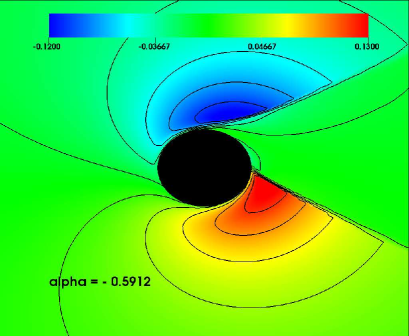
Figure 8: The radial velocity profiles for Kerr and EGB black holes with $V_{\infty}=0.2$ on the equatorial plane ($r-\phi$) a long time later after the disk reached to the steady state.

The shock cone instabilities can be calculated by performing a power mode analysis on the steady state shock cone around the black hole in Kerr and EGB gravities. This can be done by defining the azimuthal wavenumber and finding the saturation points in the oscillating system (Dönmez, 2014). The growth of the instability modes for the azimuthal wavenumber $m=1$ in case of the BHL accretion in Kerr and EGB gravities is given in Figs.9 and 10. As expected, the mode rapidly increases due to BHL accretion onto the black hole. The mode and saturation point are developed for all the values of asymptotic velocity about $t=250M$ except $V_{\infty}=0.1$ as seen in Fig.9. The power mode for asymptotic velocity $V_{\infty}=0.1$ keeps growing until $t=13000M$ and it reaches saturation. The shock cone and the disk do not show any remarkable oscillation after the system reaches a saturation in all simulations. As seen in Fig.10, the power mode analysis of the shock cone in EGB gravity shows slightly different behavior than Kerr gravity. The instability is developed at a later time in the EGB gravity and it saturates slightly later than the Kerr gravity (cf. the inset of Fig.10). In addition, we did not observed any substantial difference in the behavior of the power mode analysis for different $\alpha$. Fig.10 also shows that the instability is developed at a slightly later time than the other ones for $\alpha=-0.5912$.

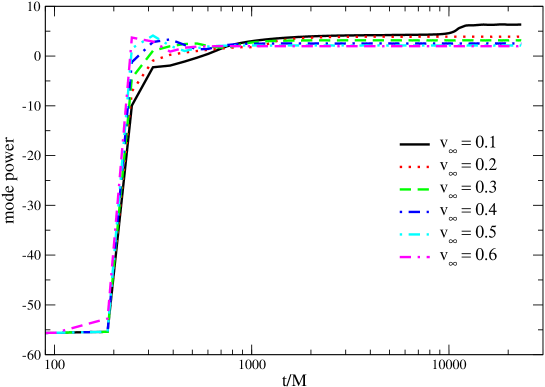
Figure 9: The evolution of $m=1$ mode power for EGB black hole with $\alpha=-0.5912$.

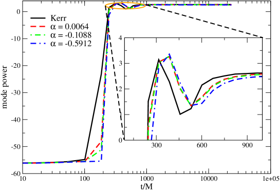
Figure 10: The evolution of $m=1$ mode power for Kerr and EGB black holes with $V_{\infty}=0.4$.

5 Astrophysical Motivation

There are possible candidates in which our numerical simulation results could be used to identify properties of disk structure and radiation properties. Firstly, the variable $X-$ ray sources are observed in nearby galaxies (Walton et al., 2011). They are ultra-luminous $X-$ ray sources and contain either intermediate black holes ($M_{BH}\sim 10^{2}-10^{5}M_{\odot}$) or massive stellar black holes ($M_{BH}\sim 30-100M_{\odot}$). NGC $1313$ $X-1$ could be a quite massive ($M_{BH}\sim 70-100M_{\odot}$), accreating close to the Eddington limit and contains a hot inner disk (Bachetti et al., 2013). The rotation parameter of NGC $1313$ $X-1$ is extreme and defined as $0.93\leq a\leq 0.96$ (Heydari-Fard & Sepangi, 2021). Secondly, MAXI $J1803-298$ is a newly discovered rapidly rotating black hole candidate with a spin parameter of $0.991$ (Feng et al., 2021). Lastly, many of the super-massive black holes examined seem to be rapidly rotating ones (Reynolds, 2019). The black hole spin parameter used in our numerical simulation for Kerr and 4D EGB black holes is $0.97$ which falls in the above observed values. The spin is an important parameter constraining the model properties and gives a new insight about accreation dynamics. Our numerical solution is also interesting to use the exploring the features of electromagnetic radiation and to constrain the black hole parameters depending on GB coupling constant $\alpha$. For example, it is possible to measure the deviation of the angular momentum of the massive stellar Kerr black hole using the continuum fitting (Bambi & Barausse, 2011). The observational constrain of EGB gravity was mainly discussed in Feng et al. (2020); Clifton et al. (2020) for various physical systems.

6 Discussion and Conclusion

In this paper, we investigate and compare BHL accreation onto the Kerr and EGB rotation black holes with the rotation parameter $a=0.97$ in a strong gravitational region using the non-axisymmetric hydrodynamical simulation. We use the perfect fluid equation of state with adiabatic index $\Gamma=4/3$. We study the effect of different values of GB coupling constants in subsonic, sonic, and supersonic flow regions to reveal the accretion disk dynamics and shock cone structure around the rapidly rotating black holes.

To reveal the shock cone structure, physical properties, and the radiation properties we have studied the mass accretion rate, the behavior of the rest-mass density, the shock opening angle, radial velocity of the flow, and power mode for different values of GB coupling constants and asymptotic velocities with a fixed value of the rotation parameter. The effect of the GB coupling constant $\alpha$ on the shock cone properties is discussed and compared with the Kerr black hole in general relativity. It is found that the shock opening angle is greater in EGB gravity for any value of $\alpha$ when we compare it with Kerr gravity. Besides, the shock opening angle decreases with increasing asymptotic velocity of Mach number in both Kerr and EGB gravities. On the other hand the accretion rates are nearly constant in all models after the steady state is reached and the amount of the rate is getting less for the greater value of $\alpha$ in negative direction. The accreation rate is the higher around the Kerr black hole than EGB black hole for any value of GB coupling constant. After the shock cone reaches to steady-state, it oscillates around a certain value. The oscillation amplitude is slightly diminished for $\alpha=-0.5912$. The high the oscillation amplitude in shock cone could be a good candidate to observe a time varying $X-$ rays in astrophysical phenomena.

The shock location of the cone which is attached to the black hole horizon is a natural physical system which transports the angular momentum of the accreating gas emerging close to the black hole. Therefore the transportation is responsible for the mass accreation onto the black hole. We find the efficiency of the accretion rate to be a strong function of the asymptotic velocity (Mach number). Even though the accretion rate exponentially decreases in the subsonic and supersonic regions, it reaches maximum value at sonic location which occurs at $V_{\infty}=0.1$. The gravitational force has a big influence in the subsonic region while the gas pressure is dominant in the supersonic region, especially far away from the strong gravitational region.

Finally, it is shown in our numerical simulations that the axisymmetric accretion disk with the shock cone around the rotating black hole in Kerr and EGB gravities generates more violent phenomena and it gets hotter at small value of $\alpha$ than the value of $\alpha=-0.5912$. The more violent model could be a good candidate to explore the physical features of the electromagnetic radiation of NGC $1313$ $X-1$ and $X-2$. The black hole spin parameter used in our numerical simulation for Kerr and 4D EGB black holes is $0.97$ which falls in the observed value of NGC $1313$ $X-1$ and $X-2$ and MAXI $J1803-298$.

References

- Abbott et al. (2016) Abbott, B. P., Abbott, R., Abbott, T. D., et al. 2016, Phys. Rev. Lett., 116, 061102, doi: 10.1103/PhysRevLett.116.061102
- Allahyari et al. (2020) Allahyari, A., Khodadi, M., Vagnozzi, S., & Mota, D. F. 2020, J. Cosmology Astropart. Phys, 2020, 003, doi: 10.1088/1475-7516/2020/02/003
- Bachetti et al. (2013) Bachetti, M., Rana, V., Walton, D. J., et al. 2013, ApJ, 778, 163, doi: 10.1088/0004-637X/778/2/163
- Bambi & Barausse (2011) Bambi, C., & Barausse, E. 2011, ApJ, 731, 121, doi: 10.1088/0004-637X/731/2/121
- Blondin (2013) Blondin, J. M. 2013, The Astrophysical Journal, 767, 135, doi: 10.1088/0004-637x/767/2/135
- Bondi & Hoyle (1944) Bondi, H., & Hoyle, F. 1944, MNRAS, 104, 273, doi: 10.1093/mnras/104.5.273
- Clifton et al. (2020) Clifton, T., Carrilho, P., Fernandes, P. G. S., & Mulryne, D. J. 2020, Phys. Rev. D, 102, 084005, doi: 10.1103/PhysRevD.102.084005
- Cruz-Osorio & Lora-Clavijo (2016) Cruz-Osorio, A., & Lora-Clavijo, F. D. 2016, MNRAS, 460, 3193, doi: 10.1093/mnras/stw1149
- Dönmez (2004) Dönmez, O. 2004, Ap&SS, 293, 323, doi: 10.1023/B:ASTR.0000044610.53714.95
- Donmez (2006) Donmez, O. 2006, AM&C, 181, 256, doi: 10.1016/j.amc.2006.01.031
- Dönmez (2012) Dönmez, O. 2012, MNRAS, 426, 1533, doi: 10.1111/j.1365-2966.2012.21616.x
- Dönmez (2014) —. 2014, MNRAS, 438, 846, doi: 10.1093/mnras/stt2255
- Donmez (2022) Donmez, O. 2022, Physics Letters B, 827, 136997, doi: 10.1016/j.physletb.2022.136997
- Dönmez et al. (2011) Dönmez, O., Zanotti, O., & Rezzolla, L. 2011, MNRAS, 412, 1659, doi: 10.1111/j.1365-2966.2010.18003.x
- Donmez, Orhan (2021) Donmez, Orhan. 2021, Eur. Phys. J. C, 81, 113, doi: 10.1140/epjc/s10052-021-08923-1
- Edgar (2004) Edgar, R. 2004, New A Rev., 48, 843, doi: 10.1016/j.newar.2004.06.001
- Event Horizon Telescope Collaboration et al. (2019a) Event Horizon Telescope Collaboration, Akiyama, K., Alberdi, A., et al. 2019a, ApJ, 875, L1, doi: 10.3847/2041-8213/ab0ec7
- Event Horizon Telescope Collaboration et al. (2019b) —. 2019b, ApJ, 875, L2, doi: 10.3847/2041-8213/ab0c96
- Event Horizon Telescope Collaboration et al. (2019c) —. 2019c, ApJ, 875, L3, doi: 10.3847/2041-8213/ab0c57
- Feng et al. (2020) Feng, J.-X., Gu, B.-M., & Shu, F.-W. 2020, arXiv e-prints, arXiv:2006.16751. https://arxiv.org/abs/2006.16751
- Feng et al. (2021) Feng, Y., Zhao, X., Li, Y., et al. 2021, arXiv e-prints, arXiv:2112.02794. https://arxiv.org/abs/2112.02794
- Foglizzo et al. (2005) Foglizzo, T., Galletti, P., & Ruffert, M. 2005, A&A, 435, 397, doi: 10.1051/0004-6361:20042201
- Gergely & Biermann (2009) Gergely, L. Á., & Biermann, P. L. 2009, ApJ, 697, 1621, doi: 10.1088/0004-637X/697/2/1621
- Glavan & Lin (2020) Glavan, D., & Lin, C. 2020, Phys. Rev. Lett., 124, 081301, doi: 10.1103/PhysRevLett.124.081301
- Gracia-Linares & Guzmán (2015) Gracia-Linares, M., & Guzmán, F. S. 2015, ApJ, 812, 23, doi: 10.1088/0004-637X/812/1/23
- Guo & Li (2020) Guo, M., & Li, P.-C. 2020, European Physical Journal C, 80, 588, doi: 10.1140/epjc/s10052-020-8164-7
- Guo et al. (2021) Guo, S., He, K.-J., Li, G.-R., & Li, G.-P. 2021, Classical and Quantum Gravity, 38, 165013, doi: 10.1088/1361-6382/ac12e4
- Gyulchev et al. (2021) Gyulchev, G., Nedkova, P., Vetsov, T., & Yazadjiev, S. 2021, European Physical Journal C, 81, 885, doi: 10.1140/epjc/s10052-021-09624-5
- Heydari-Fard et al. (2020) Heydari-Fard, M., Heydari-Fard, M., & Sepangi, H. R. 2020, European Physical Journal C, 80, 351, doi: 10.1140/epjc/s10052-020-7911-0
- Heydari-Fard et al. (2021) —. 2021, European Physical Journal C, 81, 473, doi: 10.1140/epjc/s10052-021-09266-7
- Heydari-Fard & Sepangi (2021) Heydari-Fard, M., & Sepangi, H. R. 2021, Physics Letters B, 816, 136276, doi: 10.1016/j.physletb.2021.136276
- Hoyle & Lyttleton (1939) Hoyle, F., & Lyttleton, R. A. 1939, Proceedings of the Cambridge Philosophical Society, 35, 405, doi: 10.1017/S0305004100021150
- Hunt (1971) Hunt, R. 1971, Monthly Notices of the Royal Astronomical Society, 154, 141, doi: 10.1093/mnras/154.2.141
- Karimov et al. (2018) Karimov, R. K., Izmailov, R. N., Bhattacharya, A., & Nandi, K. K. 2018, European Physical Journal C, 78, 788, doi: 10.1140/epjc/s10052-018-6270-6
- Khodadi et al. (2020) Khodadi, M., Allahyari, A., Vagnozzi, S., & Mota, D. F. 2020, J. Cosmology Astropart. Phys, 2020, 026, doi: 10.1088/1475-7516/2020/09/026
- Koyuncu & Dönmez (2014) Koyuncu, F., & Dönmez, O. 2014, Modern Physics Letters A, 29, 1450115, doi: 10.1142/S0217732314501156
- Liu et al. (2021) Liu, C., Zhu, T., & Wu, Q. 2021, Chinese Physics C, 45, 015105, doi: 10.1088/1674-1137/abc16c
- Lora-Clavijo et al. (2015) Lora-Clavijo, F. D., Cruz-Osorio, A., & Moreno Méndez, E. 2015, ApJS, 219, 30, doi: 10.1088/0067-0049/219/2/30
- Lora-Clavijo & Guzmán (2013) Lora-Clavijo, F. D., & Guzmán, F. S. 2013, MNRAS, 429, 3144, doi: 10.1093/mnras/sts573
- MacLeod & Ramirez-Ruiz (2015) MacLeod, M., & Ramirez-Ruiz, E. 2015, The Astrophysical Journal, 803, 41, doi: 10.1088/0004-637x/803/1/41
- Malafarina et al. (2020) Malafarina, D., Toshmatov, B., & Dadhich, N. 2020, Physics of the Dark Universe, 30, 100598, doi: 10.1016/j.dark.2020.100598
- Mould (2021) Mould, M. 2021, arXiv e-prints, arXiv:2104.15011. https://arxiv.org/abs/2104.15011
- Ohsugi (2018) Ohsugi, Y. 2018, Astronomy and Computing, 25, 44, doi: https://doi.org/10.1016/j.ascom.2018.08.005
- Penner (2011) Penner, A. J. 2011, Monthly Notices of the Royal Astronomical Society, 414, 1467, doi: 10.1111/j.1365-2966.2011.18480.x
- Penner (2012) —. 2012, Monthly Notices of the Royal Astronomical Society, 428, 2171, doi: 10.1093/mnras/sts176
- Pérez et al. (2017) Pérez, D., Armengol, F. G. L., & Romero, G. E. 2017, Phys. Rev. D, 95, 104047, doi: 10.1103/PhysRevD.95.104047
- Pun et al. (2008) Pun, C. S. J., Kovács, Z., & Harko, T. 2008, Phys. Rev. D, 78, 084015, doi: 10.1103/PhysRevD.78.084015
- Reynolds (2019) Reynolds, C. S. 2019, Nature Astronomy, 3, 41, doi: 10.1038/s41550-018-0665-z
- Ruffert (1994) Ruffert, M. 1994, ApJ, 427, 342, doi: 10.1086/174144
- Ruffert & Arnett (1994) Ruffert, M., & Arnett, D. 1994, ApJ, 427, 351, doi: 10.1086/174145
- Staykov et al. (2016) Staykov, K. V., Doneva, D. D., & Yazadjiev, S. S. 2016, J. Cosmology Astropart. Phys, 2016, 061, doi: 10.1088/1475-7516/2016/08/061
- Walton et al. (2011) Walton, D. J., Roberts, T. P., Mateos, S., & Heard, V. 2011, MNRAS, 416, 1844, doi: 10.1111/j.1365-2966.2011.19154.x
- Xu & Stone (2019) Xu, W., & Stone, J. M. 2019, MNRAS, 488, 5162, doi: 10.1093/mnras/stz2002
- Yuan & Narayan (2014) Yuan, F., & Narayan, R. 2014, ARA&A, 52, 529, doi: 10.1146/annurev-astro-082812-141003
- Zhang et al. (2020) Zhang, Y.-P., Wei, S.-W., & Liu, Y.-X. 2020, Universe, 6, 103, doi: 10.3390/universe6080103