Travelling Salesman Problem:
Parallel Implementations & Analysis

Abstract

The Traveling Salesman Problem (often called TSP) is a classic algorithmic problem in the field of computer science and operations research. It is an NP-Hard problem focused on optimization. TSP has several applications even in its purest formulation, such as planning, logistics, and the manufacture of microchips; and can be slightly modified to appear as a sub-problem in many areas, such as DNA sequencing. In this paper, a study on parallelization of the Brute Force approach (under several paradigms) of the Travelling Salesman Problem is presented. Detailed timing studies for the serial and various parallel implementations of the Travelling Salesman Problem have also been illustrated.

I Introduction

The Travelling Salesman Problem (TSP) is the challenge of finding the shortest yet most efficient route for a person to take given a list of specific destinations along with the cost of travelling between each pair of destinations.

Stated formally, given a set of $N$ cities and distances between every pair of cities, the problem is to find the shortest possible route that visits every city exactly once and returns to the starting point. The problem is an NP-Hard problem that is, no polynomial-time solution exists for this problem. The brute force solution for the problem is to consider $city_{1}$ as a starting city and then generate all the permutations of the remaining $N-1$ cities and return the permutation with the minimum cost. The time complexity for this solution is $O(N!)$. Another solution using the Dynamic programming paradigm exists with the time complexity $O(N^{2}2^{N})$ which is much less than $O(N!)$ but it has exponential space complexity so impractical to implement.

The goal of this study is to parallelize the Brute Force algorithm for solving TSP using a variety of paradigms (using OpenMP, MPI & CUDA), and to critically compare and analyse the differences in their performance.

II Serial Implementation of Brute Force TSP

Representing a TSP tour is rather simple. It is just a permutation of the cities, with the added restriction that the first city must always be $city_{1}$. Once we realize that each of the tours is a permutation, then a brute-force algorithm that is guaranteed to always solve the TSP becomes evident: Examine all possible permutations of cities, and keep the one that is shortest. The pseudo-code for this approach has been outlined in Algorithm 1.

The number of permutations made using $city_{1},city_{2},...,city_{N}$ is given by $N!$ Since we only want those permutations with $city_{1}$ as the first destination, we are left with $(N-1)!$ permutations to explore. Hence, iterating through the permutations takes $O((N-1)!)$ time.

Algorithm 1 Brute Force Serial TSP

  Input: $city\_list$, $cost\_matrix$

  $optimal\_cost\leftarrow\infty$

  $optimal\_path\leftarrow null$

  $city\_list\leftarrow list\ of\ cities\ excluding\ city_{1}$

  while $next\_permutation(city\_list)$ do

     $temp\_cost\leftarrow get\_path\_cost(city\_list,cost\_matrix)$ {Cost of travelling cities in order of cities in $city\_list$}

     if $temp\_cost<optimal\_cost$ then

        $optimal\_cost\leftarrow temp\_cost\$

        $optimal\_path\leftarrow$$city\_list$ {with $city_{1}$ appended at start & end}

     end if

  end while

  Output: $optimal\_path$, $optimal\_cost$

Now, calculating the cost for $N$ cities in the path for each permutation requires traversal of an array of length $N$, which takes $O(N)$ time. Hence, this brute force algorithm takes $O((N-1)!\times N)=O(N!)$ time.

Algorithm 1 shows the use of the $next\_permutation(...)$ function that takes in a list of destinations, i.e., $city\_list$ & checks if there exists a next lexicographic permutation for the given permutation of destinations. If it does exist, modify $city\_list$ to store this next permutation, so that it may be used to calculate the path cost. The $get\_path\_cost(...)$ function calculates the cost of travelling through the cities based on the order mentioned in $city\_list$, & finding the individual trip costs from the $cost\_matrix$. At the end, we would have exhausted all possible $(N-1)!$ permutations & arrive at the optimal path with the least path cost.

This serial implementation of Brute Force TSP can be found in tsp.cpp file.

III Motivation to Parallelize Brute Force TSP

We notice that all the major computations required for finding the optimal path in this brute force approach need to be done for every permutation. Clearly, parallelizing the iteration over these permutation of destinations makes this problem almost embarrassingly parallelizable under brute force search.

Thus, our project involves the implementation of this brute force TSP algorithm under different paradigms using:

• OpenMP (Shared Memory Processing)

• MPI (Message Passing Interface)

• CUDA (for NVIDIA GPUs)

Further, our analysis focuses on the comparison between the time taken for the serial algorithm & its various parallel counterparts, while also trying to explain the parallelizability of the algorithm.

IV System Specifications for Experiments

All the code execution & timing studies have been performed on Param Sanganak. Tables I & II summarize the specifications of the execution environment.

Architecture	x86_64
CPU op-mode(s)	32-bit, 64-bit
Byte Order	Little Endian
CPU(s)	40
Thread(s) per core	1
Core(s) per socket	20
Socket(s)	2
Model Name	Intel(R) Xeon(R) Gold
	6248 CPU @ 2.50GHz
CPU MHz	999.908
GPU Model	Tesla V100-SXM2-16GB
GPU Bus Type	PCIe
GPU DMA Size	47 bits

TABLE I: Hardware Specifications on Param Sanganak

Operating System	CentOS 7.6
g++ Version	4.8.5
OpenMP Version	3.1
MPI Version	4.0.2rc3
CUDA Version	11.1

TABLE II: Software Specifications on Param Sanganak

V OpenMP (Shared Memory Processing)

V-A Approach for Parallelization

For parallelizing the brute force approach for TSP using OpenMP, all the different permutations of cities are consider and are divided equally (in case number of threads divide number of permutations exactly) among different sections based on threads, however if number of threads does not exactly divide number of permutations, the first r (remainder on division) threads are given one extra permutation to compute. Now, to maintain continuity between two consecutive threads, the initial arrangements of cities are given to each section based on thread IDs and then consequent arrangements are computed within the thread itself. Each thread now calculates its respective optimal cost and path, by looping between the starting and ending permutation (for each thread) and then comparing the optimal values and path of all the threads. This implementation can be found in tsp_omp.cpp file.

V-B Timing Analysis

Figures 1 & 2 illustrate the time taken for execution and speedup achieved for the OpenMP parallelization approach for different number of threads and number of cities (N).

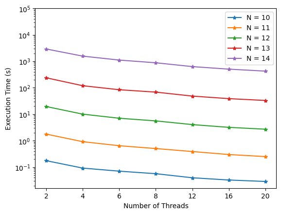
Figure 1: Variation of execution times with number of OpenMP threads for different problem sizes ($N=$ Number of cities)

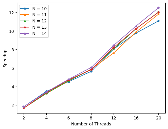
Figure 2: Variation of speedup achieved with number of OpenMP threads for different problem sizes ($N=$ Number of cities)

• Execution time decreases with increase in # of threads.

• The difference between the execution time for two consecutive cities is large because it depends on $N!$.

• Speedup increases with increase in the number of threads, while the trend remains similar across all $N^{\prime}s$.

VI MPI (Message Passing Interface)

VI-A Approach for Parallelization

For parallelizing the brute force approach for TSP using MPI (Message Passing Interface), the permutations of cities are equally divided among available Parallel Environments (PEs), while taking care of the case where equal distribution is not possible. The data of edge weights is distributed across all PEs, followed by synchronization. Each PE is given a starting permutation index and an ending permutation index. Calculation of these permutation indices are done so as to take care of the cases when equal distribution of permutations is not possible, and therefore, remainder work is further divided across PEs. Each PE now calculates its respective optimal cost and path, by looping through the starting to ending permutation, following the same procedure as in serial algorithm. For each PE, we have their individual respective variables to calculate optimal path and optimal value from among the permutations assigned to them. Now, all PEs are synchronized and optimal costs and paths of all PEs are compared in the Master PE. This implementation can be found in tsp_mpi.cpp file.

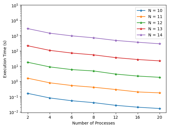
Figure 3: Variation of execution times with number of MPI processes for different problem sizes ($N=$ Number of cities)

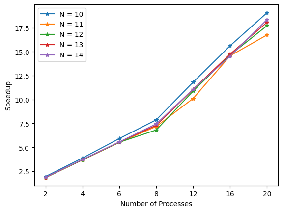
Figure 4: Variation of speedup achieved with number of MPI processes for different problem sizes ($N=$ Number of cities)

VI-B Timing Analysis

Figures 3 & 4 illustrate the time taken for execution and speedup achieved for the MPI parallelization approach for different number of Parallel Environments (PEs) and number of cities ($N$).

• Execution time decreases with increase in # of PEs.

• The difference between the execution time for two consecutive cities is large because it depends on $N!$.

• Speedup increases with increase in the number of PEs, while the trend remains similar across all $N^{\prime}s$.

VII Comparative Study of OpenMP & MPI

Based on the Timing Analysis of the OpenMP & MPI implementations, we conclude that the speedups achieved through Message Passing (i.e., MPI) are greater than those achieved through Shared Memory (i.e., OpenMP). This is apparent from the fact that using 20 PEs (in MPI) results in speedups of $\sim 18$, while using 20 threads (in OpenMP) results in speedups of merely $\sim 12$.

		No. of Threads (p)
		2	4	8	16	20
N	10	0.907	0.865	0.704	0.610	0.554
	11	0.834	0.808	0.734	0.618	0.590
	12	0.834	0.810	0.729	0.639	0.601
	13	0.834	0.831	0.726	0.640	0.600
	14	0.909	0.848	0.750	0.658	0.618

TABLE III: Efficiency ($\eta$) of the OpenMP implementation for various $N$ (problem size) & $p$ (no. of OpenMP threads)

		No. of PEs (p)
		2	4	8	16	20
N	10	0.975	0.970	0.984	0.976	0.953
	11	0.922	0.920	0.898	0.910	0.838
	12	0.918	0.922	0.851	0.916	0.886
	13	0.927	0.929	0.913	0.921	0.904
	14	0.934	0.931	0.931	0.908	0.918

TABLE IV: Efficiency ($\eta$) of the MPI implementation for various $N$ (problem size) & $p$ (no. of MPI Processes)

This is also evident by comparing the efficiencies of OpenMP & MPI implementations shown in Tables III & IV. Clearly, the efficiency for MPI code is always greater than its OpenMP counterpart. This is potentially due to extra overheads of spawning & maintaining OpenMP threads compared to the inter-process communications in MPI.

We also calculate the Karp-Flatt Metric, or experimentally determined serial fraction $e(N,p)$ of parallel computation for both these implementations. Given the speedup $\Psi(N,p)$ using $p$ processors, $e(N,p)$ is determined as follows:

$$e(N,p)=\frac{\frac{1}{\Psi}-\frac{1}{p}}{1-\frac{1}{p}}$$

		No. of Threads (p)
		2	4	8	16	20
N	10	0.103	0.052	0.060	0.043	0.042
	11	0.199	0.079	0.052	0.041	0.037
	12	0.199	0.078	0.053	0.038	0.035
	13	0.198	0.068	0.054	0.037	0.035
	14	0.100	0.060	0.048	0.035	0.033

TABLE V: $e(N,p)$ of the OpenMP implementation for various $N$ (problem size) & $p$ (no. of OpenMP threads)

		No. of PEs (p)
		2	4	8	16	20
N	10	0.025	0.010	0.002	0.002	0.003
	11	0.085	0.029	0.016	0.007	0.010
	12	0.089	0.028	0.025	0.006	0.007
	13	0.078	0.026	0.014	0.006	0.006
	14	0.070	0.025	0.011	0.007	0.005

TABLE VI: $e(N,p)$ of the MPI implementation for various $N$ (problem size) & $p$ (no. of MPI Processes)

Tables V & VI show $e(N,p)$ for OpenMP & MPI respectively. The following inferences can be made:

• For a given $N$, $e(N,p)$ usually decreases or remains constant with increase in $p$, indicating that the brute force TSP algorithm is rather embarrassingly parallel.

• Comparing the corresponding $e(N,p)$ values for OpenMP & MPI, highlights that OpenMP code contains higher fraction of serial component, leading to lower speedups.

VIII Hybrid Approach (Combining MPI & OpenMP)

VIII-A Approach for Parallelization

After comparing the MPI & OpenMP approaches, we implemented a hybrid approach by combining the two & analysed its performance. This involved the spawning of multiple OpenMP threads ($num\_threads$) in each of the multiple MPI processes ($num\_PEs$) such that the permutations were divided equally among the $num\_PEs\times num\_threads$ parallel elements (while addressing the cases of unequal division). The code for this approach has been implemented in tsp_hybrid.cpp.

VIII-B Timing Analysis

Keeping the total number of parallel elements same, increasing the number of MPI processes & decreasing the number of OpenMP threads reduces the execution time. This can be explained by the larger overheads of maintaining OpenMP threads compared to the MPI communication overhead. A glimpse of this trend can be seen in Table VII.

However, using lesser number of PEs (with same total parallel elements) proves to be worse even compared to OpenMP, perhaps due to the higher costs of maintaining threads & their synchronization across only a small number of PEs. Once the number of PEs becomes large enough, thread maintenance costs are overcome by MPI communication.

Parallelization Paradigm		Execution Time (s)
OpenMP (20 threads)		32.934
MPI (20 PEs)		21.866
Hybrid	2 PEs $\times$ 10 threads	124.736
	4 PEs $\times$ 5 threads	62.219
	5 PEs $\times$ 4 threads	50.492
	10 PEs $\times$ 2 threads	25.822

TABLE VII: Comparison of hybrid code execution times against OpenMP & MPI codes with same number of parallel elements ($20$) for $N=13$

IX CUDA (NVIDIA GPUs)

IX-A Approach for Parallelization

For parallelizing the brute force approach for TSP using CUDA, we leverage both: blocks & threads. For our analysis, we use 50 blocks, each with 1024 threads. We divide the permutations of cities among the threads in all the blocks. Each thread in a block calculates the minimum cost path from the assigned permutations. After synchronizing the threads in each separate block, one thread (with Thread ID = 0) computes the optimal cost & path for the block, and stores it in a shared global data structure that can be accessed by both GPU and CPU. Once the GPU finishes execution, the host calculates the optimal path by iterating over the minimum cost path of each block stored in the previously mentioned data structure. This implementation can be found in tsp_cuda.cu file.

IX-B Timing Analysis

Table VIII summarizes the time taken for execution and speedup achieved by leveraging the power of NVIDIA GPU.

N	Time (s)		Speedup
	Serial Code	CUDA Code
8	0.004	0.017	0.264x
9	0.065	0.042	1.537x
10	0.316	0.020	15.725x
11	2.9416	0.057	51.278x
12	32.440	0.048	673.260x
13	395.165	0.086	4557.187x
14	5289.317	0.822	6427.022x
15	74060 ($\sim$ 20 hr)	9.753	7590x
16	1110900 ($\sim$ 308 hr)	151.387	7340x
17	$\sim$ 4936 hr	1867.08	9520x

TABLE VIII: Execution times & speedups achieved using CUDA for various values of $N$

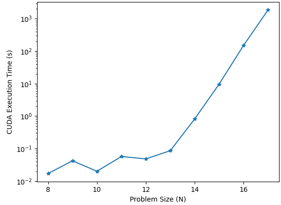
Figure 5: Plot of CUDA execution time w.r.t problem size ($N$)

Figure 5 also shows the variation of CUDA execution time with increase in problem size $N$. We were restricted by the maximum capacity of C++ primitive datatypes (for storing the factorial values) to keep our analysis only upto $N=17$.

Some observations made from the above study include:

• As $N$ increases, it is evident that the GPU provides immense benefits through parallelization, as we obtain speedups of great magnitudes.

• For large $N$ ($\geq 15$), it was infeasible to run the serial code due to the estimated total time based on the $O(N!)$ nature of the algorithm.

• For $N\geq 13$, even though the speedups are huge, the actual CUDA execution time increases exponentially because $N!$ becomes overwhelmingly large to be parallelized across $50\times 1024$ threads.

• Following the trend, if $N=18$, the serial execution could take around $83900$ hrs. Now, even if we extrapolate the speedups to $\sim 10000$x, the CUDA code will still require $8+$ hrs to execute, which is unacceptably large.

• This analysis clearly illustrates the imperative need to choose an efficient algorithm to solve a problem instead of trying to parallelize an inefficient algorithm.

X Conclusions & Future Work

In this project, we explore the Travelling Salesman Problem & implement several approaches to parallelize the Brute Force TSP algorithm, including OpenMP, MPI & CUDA programming. We perform detailed timing analysis for all the approaches & also critically compare the performance of OpenMP & MPI codes through their efficiency & Karp-Flatt metric. We also develop and analyse a hybrid parallel algorithm leveraging both OpenMP & MPI.

This project can be extended to parallelize & compare other algorithms to solve the TSP such as Branch-&-Bound, Genetic Algorithms, etc. This would provide a better idea about the relative importance of selecting a good algorithm & parallelizing an algorithm.

References

1. Understanding The Travelling Salesman Problem (TSP)

2. Burkhovetskiy, V. & Steinberg, B.; Parallelizing an exact algorithm for the traveling salesman problem; Procedia Computer Science, Volume 119, Pg 97-102 - 2017

3. Izzatdin, Abdul & Haron, Nazleeni & Mehat, Mazlina & Low, Tang & Nabilah, Aisyah. (2008). Solving traveling salesman problem on high performance computing using message passing interface.

4. Sharing global and local variables using Unified Memory in CUDA

5. Karp-Flatt Metric