Differentiable Point-Based Radiance Fields
for Efficient View Synthesis

Abstract.

We propose a differentiable rendering algorithm for efficient novel view synthesis. By departing from volume-based representations in favor of a learned point representation, we improve on existing methods more than an order of magnitude in memory and runtime, both in training and inference. The method begins with a uniformly-sampled random point cloud and learns per-point position and view-dependent appearance, using a differentiable splat-based renderer to train the model to reproduce a set of input training images with the given pose. Our method is up to 300 $\times$ faster than NeRF in both training and inference, with only a marginal sacrifice in quality, while using less than 10 MB of memory for a static scene. For dynamic scenes, our method trains two orders of magnitude faster than STNeRF and renders at a near interactive rate, while maintaining high image quality and temporal coherence even without imposing any temporal-coherency regularizers.

1. Introduction

Neural rendering has emerged as an effective tool to model real-world scenes [Mildenhall et al., 2020], synthesize novel views [Lombardi et al., 2019], and advance single-shot learning [Yu et al., 2021c]. Specifically, existing work has made it possible to generate photorealistic novel views at unseen viewpoints from unorganized multi-view training images. Synthesizing novel views could not only enable after-shot visual effects in consumer photography and virtual reality but also implicitly/explicitly entails the geometric understanding of a scene. Utilizing an efficient view-synthesis network in an analysis-by-synthesis framework may further allow these techniques to become the missing link for inverse-rendering applications in diverse application domains.

Neural radiance fields (NeRF) [Mildenhall et al., 2020] have spearheaded neural rendering by modeling a 5D radiance field in a memory-efficient manner with an implicit scene representation in the form of a multi-layer perceptron (MLP). A large body of work has built on this method using implicit scene representations for view synthesis, investigating generalizability [Yu et al., 2021c] and rendering quality [Wizadwongsa et al., 2021]. However, a drawback of modern neural rendering methods is their computational efficiency. As NeRF relies on volumetric rendering, training and inference of a model requires many evaluations and memory accesses of the radiance fields: typically more than 100 evaluations for each ray. As a result, for medium-sized static scenes, NeRF takes over ten hours of training and 30 seconds of inference for each scene on a single GPU. The limited computational efficiency of NeRF-based methods prevents the direct applicability to video applications, where fast training and inference at a low memory footprint are mandated. Recent methods have attempted to tackle this problem by pretraining a multi-view stereo model on a large-scale dataset and fine-tuning it for test inputs [Chen et al., 2021b], or using an explicit radiance volume [Yu et al., 2021b]. While these methods outperform NeRF in efficiency, they are not capable of accelerating both training and inference speed and require a large pretraining dataset as well as significant storage.

In this work we explore an alternative approach for retaining the highly-desirable end-to-end differentiability of NeRF, while utilizing an alternate radiance field representation. Our insight is that, even though the MLP used by NeRF is compact and relatively efficient to evaluate once, using it for image synthesis is fundamentally a “backward mapping” operation that requires multiple evaluations of radiance along a ray. Shifting to a representation that allows “forward mapping,” i.e., creating an image via a single forward pass over the representation of the radiance field, enables modest gains in storage but, more importantly, efficiency gains of multiple orders of magnitude at both training and rendering time.

Specifically, we use a representation for radiance based on RGB spherical harmonic coefficients stored at points in 3D. Image synthesis is then accomplished via a differentiable splat-based rasterizer that operates as a single forward pass. The rendering pipeline from point primitives and spherical harmonic coefficients to images is end-to-end differentiable, allowing for optimizing the position and appearance attributes with a coarse-to-fine first-order optimization method.

Our strategy yields several benefits: smaller storage, faster training, and more efficient rendering that avoids volumetric ray marching. The cost is reduced flexibility in radiance representation, but this is not always a drawback. Indeed, with few input views, the regularization provided by our method leads to higher reconstruction quality. However, when many input views are provided, our method results in slightly lower quality (for a fixed spherical harmonic degree). Our approach learns point clouds with position and appearance without a neural network or separate geometry estimation (e.g., via COLMAP) step. As such, it allows for efficient inference and training.

Specifically, we make the following contributions in this work:

• We introduce a point-based radiance representation that, together with differentiable splatting, is 300 $\times$ faster than neural volumetric methods for view synthesis in both training and inference.

• We analyze the proposed point-cloud representation in terms of memory, inference and training run-time, and show that it outperforms state-of-the-art neural rendering algorithms [Yu et al., 2021a] in compute while being two orders of magnitude smaller in memory.

• We demonstrate that our method is efficient enough in memory, training time, and rendering time to enable novel-view synthesis for video, even without establishing explicit frame-to-frame connections. We validate that the proposed method outperforms existing methods in quality, run time, and memory footprint.

We have released all code and data required to reproduce the findings from this work. Here is the link.

Limitations

The proposed method requires an object mask to generate the initial point cloud, and thus can only render the foreground scene components. This limitation may be potentially lifted by replacing the hard multi-view consistency function with a soft one: setting a threshold to filter based on projected pixel variance. As popular existing multi-view and video datasets contain masks, we leave such a potential extension for future work. The proposed representation which relies on splatting can also not handle semi-transparent objects, e.g., objects with fur.

2. Related Work

Neural Rendering

A rapidly growing body of work investigates introducing differentiable modules into rendering approaches, turning conventional rendering methods into powerful inverse tools for capturing, reconstructing, and synthesizing real-world scenes. Among many rendering principles, volumetric rendering has been actively studied in conjunction with neural networks [Mildenhall et al., 2020] thanks to its learning-friendly structure. In this context, various network architectures have been proposed to model scene radiance, including convolutional neural network (CNN) in Neural Volumes [Lombardi et al., 2019] and multi-layer perceptron (MLP) in NeRF [Mildenhall et al., 2020]. While the synthesized images from these methods achieve unprecedented fidelity, one of the drawbacks is their generalization ability. To tackle this challenge, image features can be explicitly exploited either from a single image [Yu et al., 2021c] or multiple images [Wang et al., 2021; Chen et al., 2021b; Liu et al., 2021]. Another line of neural-rendering methods utilizes a multi-plane image (MPI) as a scene representation for high-quality view synthesis [Zhou et al., 2018; Wizadwongsa et al., 2021]. Lastly, using point clouds has been studied for neural rendering with iterative filtering [Rosenthal and Linsen, 2008] and multi-scale approaches [Marroquim et al., 2007; Meshry et al., 2019; Rückert et al., 2021]. Among the many successful approaches, NeRF-based volumetric methods in particular have achieved remarkable success.

However, volumetric methods are not without limitations, and one major problem is their computational efficiency. While occupying only a small memory footprint, NeRF-based models typically require hours of training in a modern GPU, and inference takes minutes. This low computational efficiency prevents NeRF methods from being used in applications that require fast training and inference. Recently, researchers devised methods to accelerate inference, at the cost of additional memory incurred: Garbin et al. [2021] cache explicit volumes, Yu et al. [2021b] propose an octree structure, and Reiser et al. [2021] replace a large MLP with multiple small-size MLPs. Although these methods can speed up the rendering process, the training is still volumetric, making existing approaches slow. Recently, Lombardi et al. [2021] proposed a hybrid scene representation with primitive-based and volumetric components. As such, this method inherits some of the drawbacks of volumetric methods, including training time: this work requires 5 days of training time for a single scene, orders of magnitude more than the proposed method. Hedman et al. [2021] propose a post-training approach for fast rendering with NeRFs and Neff et al. [2021] introduce the use of depth oracle to speed up the model training speed. Yu et al. [2021a] use explicit volumes instead of an MLP and directly optimizes the volume parameters. However, this results in gigabytes of memory consumption for each scene, hence an inevitable explosion with terabytes of memory for multi-frame video. In this work, we propose a computationally-efficient rendering method that accelerates both training and inference, achieving 2 $\times$ faster inference, 3 $\times$ faster training, and 100 $\times$ lower memory footprint than Yu et al. [2021a].

Figure 2. Learning Point-Based Radiance Fields. The proposed method learns a point cloud augmented with RGB spherical harmonic coefficients per point. Image synthesis is accomplished via a differentiable splat-based rasterizer that operates as a single forward pass, without the need for ray-marching and hundreds of evaluations of coordinate-based networks as implicit neural scene representation methods. Specifically, the point rasterizer computes an alpha value from the ray-point distance with a Gaussian radial basis function weight. The learnable radiance and the alpha values are rasterized via alpha blending to render the image. The entire rendering pipeline is differentiable and we optimize for the point position and spherical harmonic coefficients end-to-end. We use a hybrid coarse-to-fine strategy (bottom) to train the entire model and successively refine the geometry represented by the learned point cloud.

Multi-view Geometry Reconstruction

Our work falls into the category of multi-view geometry reconstruction methods studied for decades in computer graphics and vision. This direction traces back to popular multi-view stereo methods using local photometric consistency and global visibility constraints [Furukawa and Ponce, 2009] and geometric priors [Schönberger et al., 2016]. Recently, neural networks have accelerated multi-view geometry acquisition [Yao et al., 2018; Im et al., 2019; Han et al., 2020]. Notably, Han et al. [2020] use multi-view projection and exploit silhouette images to estimate shape, demonstrating state-of-the-art performance. Recently, Wiles et al. [2020] (SynSin) and Thonat et al. [2021] propose single-shot video prediction and mesh-based multi-view video methods with technical approaches orthogonal to ours. Specifically, none of these existing methods can model the geometry and radiance simultaneously. In addition, they typically require a separate dataset to pretrain the model for a geometry prior. The proposed method optimizes a learned point cloud directly for each scene that does not require additional learned or explicit priors. Recent work [Kondo et al., 2021] explores how knowledge of the visual hull can help accelerate the neural rendering process, and this method cannot improve inference time.

View-dependent Modeling and Rendering

Modeling and rendering view-dependent scene radiance has been studied extensively in graphics and vision. Surface light fields [Wood et al., 2000] is based on a view-dependent level-of-detail rendering for meshes with subdivision connectivity. Using spherical harmonics in this context has been proposed as an effective way to represent a view-dependent function, with broad adoption in rendering and modeling [Cabral et al., 1987; Sillion et al., 1991; Ramamoorthi and Hanrahan, 2001a, b; Basri and Jacobs, 2003; Sloan et al., 2003, 2002]. Recent works apply view-dependent models to reflectance [Chen et al., 2021a; Sztrajman et al., 2021] via implicit BRDF modeling and use spherical harmonics to describe view-dependent radiance distribution [Yu et al., 2021b; Wizadwongsa et al., 2021]. The proposed method also uses spherical harmonics to model view-dependence while maintaining a lightweight and efficient model.

Point-based Rendering

Point-based rendering via splatting has been explored for decades, offering computational efficiency as an elegant scene representation [Pfister et al., 2000; Zwicker et al., 2001; Zwicker et al., 2004; Zwicker et al., 2002]. Recent works explore combining deep learning with surface splatting, e.g., Yifan et al. [2019] propose a differentiable algorithm for point-based surface and normal processing and does not have an appearance model and does not produce radiance outputs. In contrast, the proposed method optimizes for point positions and spherical harmonic coefficients in an end-to-end fashion, and it focuses on high-quality image-based rendering and novel view synthesis. Aliev et al. [2020] propose a point-based rendering method that requires a given point cloud aggregated from RGB-D captures, while the proposed method optimizes for point clouds from RGB-only inputs. In contrast to our network-free method, this method also uses a rendering network that requires a day of training time. Lassner et al. [2021] generate features by rasterization of spheres in a deferred neural rendering approach using an image-to-image rendering network (Pix2PixHD). The proposed method synthesizes an RGB image directly by splatting a point cloud with a per-point appearance model. We report in this manuscript that this results in an order of magnitude faster training time while providing better results. Kopanas et al. [2021] use rasterized encoded point clouds with features provided by conventional structure-from-motion methods, i.e., using COLMAP to build a dense point cloud, and SIBR for the depth and normal maps. A neural network then translates features into images for novel views. The feature encoding and decoding are learned, leading to long training times. Moreover, their inference stage selects image features from the training set and thus needs to store all these training features, resulting in storage requirements of multiple gigabytes in contrast to less than ten megabytes for the proposed method. Similarly, Rückert et al. [2021] assume known point clouds, recovered by COLMAP. Given a point cloud, their method employs a deferred neural rendering approach similar to Lassner et al. [2021] but with a multi-scale feature-to-image transfer network. In contrast to the proposed method that requires a few minutes of training time, Rückert et al. train for 12 hours. Very recently, Point-NeRF [Xu et al., 2022] proposes a point-based rendering method, which, in contrast to the proposed method, is not network-free and relies on relatively slow volume-rendering. As such, the rendering time of Point-NeRF is comparable to NeRF, about 400x slower than the proposed method.

3. Differentiable Point Radiance Fields

In this section, we describe the proposed differentiable point-based rendering method, which is illustrated in Fig. 2. We assume a set of images $I_{j}$, $j=1\ldots N$ as input, with known camera intrinsics and extrinsics. We learn a model of the scene as a point cloud with a per-point radiance model based on spherical harmonics. Learning minimizes the difference between the rendered scene and the original images, by updating the position and appearance of each point. The use of a differentiable splat-based rasterizer allows for gradient-based updates, while being orders of magnitude more efficient than an implicit volume-based renderer. The point cloud, the proposed method is operating on, is optimized end-to-end in a coarse-to-fine iterative fashion, starting from a rejection-sampled initial point cloud. We describe the components of the proposed method in the following.

Figure 3. Synthetic View Synthesis for Static Scenes. We represent two synthetic scenes [Mildenhall et al., 2020] with the proposed point-based radiance model. Trained only in a few minutes on multi-view images, the proposed method achieves rendering quality comparable to state-of-the-art volumetric rendering approaches such as Plenoxels [Yu et al., 2021b], while being more than 3 $\times$ faster in training, 2 $\times$ faster in inference and 100 $\times$ less memory-hungry.

3.1. Point-Based Scene Radiance

We model the scene as a set of points $P_{i}=(x_{i},y_{i},z_{i})^{\intercal}$, $i=1,\ldots,n$, with the parameters $H_{i}$ of a view-dependent radiance model per point. These 3D positions and radiance model parameters serve as the unknowns that will be updated by the optimization method to reconstruct the scene.

Geometric Model

Each 3D point $P_{i}$ projects to a 2D position $p_{i}^{j}$ in each image $I_{j}$. To model the projection operation, we assume that we know the extrinsic rigid-body transform $(R_{j},t_{j})$ and intrinsic matrix $M_{j}$ for each camera, and then compute

(1) $$p_{i}^{j}=\left(M_{j}(R_{j}P_{i}+t_{j})\right)^{\downarrow},$$

where $\left(x,y,z\right)^{\downarrow}=(x/z,y/z)$ denotes the perspective divide. Here $P_{i}$ are represented as the learnable neural parameters. Note that visibility is resolved by the rendering stage (see Section 3.2) via depth sorting and alpha blending.

Photometric Model

We model the view-dependent radiance of each point with spherical harmonics [Cabral et al., 1987] up to a maximum degree $l_{\textrm{max}}$:

(2) $$H_{i}=\{h_{i,lm}\;|\;0\leq l\leq l_{\textrm{max}},\;-l\leq m\leq l\}.$$

Note that $h_{i,lm}$ here are learnable. If we then denote the view direction of point $i$ in image $j$ as

(3) $$v_{i}^{j}=\frac{R_{j}P_{i}+t_{j}}{\|R_{j}P_{i}+t_{j}\|},$$

we can represent the color of the point in that image as

(4) $$c_{i}^{j}=\sum_{l=0}^{l_{\textrm{max}}}\sum_{m=-l}^{l}h_{i,lm}\,Y_{l}^{m}(v_{i}^{j}).$$

Point Cloud Initialization

We initialize points randomly within the visual hull defined by the image-space masks. Specifically, we use a rejection sampling method in which we uniformly sample random 3D points, project them into each image, and keep them only if they fall within all the masks. We initialize the point appearance by sampling the spherical harmonics parameter from the normal distribution with zero mean and standard deviation of one.

Our method is thus dependent on the availability and quality of the initial masks. However, we found that the optimization still produces good results if the masks are inaccurate or there are concavities not modeled by the visual hull. Further details on initialization are provided in the Appendix.

3.2. Differentiable Splat Rendering

Given a point cloud model, we render an image via point splatting, see Zwicker et al. [2001] for background on splatting methods. Specifically, we use an image-space radial basis function (RBF) kernel to represent the contribution of each point $p_{i}^{j}$ to each pixel $u$ in image $j$. We employ a Gaussian kernel of radius $r$, computing the opacity as

(5) $$\alpha_{i}^{j}(u)=\frac{1}{\sqrt{2\pi r^{2}}}\,e^{-\frac{\|p_{i}^{j}-u\|^{2}}{2r^{2}}}.$$

After obtaining the $\alpha$ map, we sort the points by $z$-distance and compute the final rendered image $\hat{I}_{j}$ via alpha blending from front to back. That is, we compute

(6) $$\hat{I}_{j}(u)=\sum_{i=1}^{n}A_{i}^{j}(u)\,c_{i}^{j},$$

where $A_{i}^{j}(u)$ represents the net contribution of the $i$-th point:

(7) $$A_{i}^{j}(u)=\alpha_{i}^{j}(u)\,\prod\limits_{k=1}^{i-1}\left(1-\alpha_{k}^{j}(u)\right),$$

where the points are taken as sorted front-to-back and $c_{i}^{j}$ is the per-point color computed via Eq. 4. Note that, as an optimization, we only consider points within a certain maximum distance of $u$ with non-negligible opacity.

3.3. Point Cloud Training

To train a point cloud model that predicts the image $I_{j}$, we employ a loss function consisting of an MSE and total variation loss, that is

(8) $$\mathcal{L}=\sum_{j=1}^{N}||I_{j}-\hat{I}_{j}||_{2}^{2}+\lambda TV(\hat{I}_{j}).$$

The total variation term represents the conventional anisotropic total variation penalty $TV(\cdot)=|\nabla_{x}\cdot|_{1}+|\nabla_{y}\cdot|_{1}$, that is the $\ell_{1}$-norm of the predicted image gradients. Since the loss function, splatting rasterizer, and point cloud geometric and photometric models are all fully differentiable, we are able to learn the point positions and their parameters end-to-end using stochastic gradient descent optimization.

To train the method we propose a non-synchronous learning strategy for optimizing the point position and harmonics parameters. Specifically, the initial learning rate for the spherical harmonics radiance model and the point positions are $3e-3$ and $8e-4$, respectively. Both of them are exponentially decayed for every epoch (20 epochs in total) with a factor of $0.93$. The TV weight $\lambda$ is set to $0.01$. The splatting radius $r$ and the rasterization $n$ are set as $0.008$ and $15$ respectively. We use $l_{\textrm{max}}=2$ for all of the results in the paper, since in our experiments using a higher degree resulted in a minimal quality gain for significant extra storage and training time. Section 4.3 contains an ablation study comparing spherical harmonics to just a single color, which effectively corresponds to $l_{\textrm{max}}=0$.

Hybrid Coarse-to-Fine Updates

To learn an accurate point cloud representation, we repeat the following several stages of a coarse-to-fine scheme twice, also illustrated in Fig. 2:

1. Voxel-based Point Cloud Reduction: We assume a voxel discretization (without actually voxelizing the scene), and, for each voxel, we aggregate all the points inside that voxel into one single point by averaging the position and the spherical harmonics of these points. The motivation behind this step is to avoid the formation of dense point clusters and improve the representation efficiency.

2. Outlier Removal: For each point, we compute the distance to its neighbors and the standard deviation of these distances. We then filter out the outliers whose standard deviation is beyond a threshold, hence removing outlier points.

3. Point Generation: In this stage, we insert new points into the point cloud by generating a single new point for each point in the point cloud. We set all parameters (including position) to the average of the point’s nearest $K$ neighbors.

We refer to Alg. 1 for this coarse-to-fine update in the Appendix. As a final step, we fine-tune the model with half of the original learning rate in a refinement step.

Table 1. Static Novel View Synthesis Evaluation on the Synthetic Blender Dataset. We evaluate the proposed method and comparable baseline approaches for novel view synthesis on the static Blender scenes from [Mildenhall et al., 2020]. The proposed model does not require an extra dataset for pretraining and improves on existing methods in training, inference speed and model size, at cost of only a small reduction in quality. Specifically, although the concurrent Plenoxels [2021a] achieves better quality, our model is two magnitudes smaller than theirs. We also compare here to the Plenoxels_s model from [Yu et al., 2021a] (Plenoxels with smaller volume resolution), which achieves worse rendering quality with a larger model size.

Synthetic Dataset	Pretraining	Training	Inference	Model Size	Rendering Quality
					PSNR$\uparrow$	SSIM$\uparrow$	LPIPS$\downarrow$
NeRF [Mildenhall et al., 2020]	None	20 h	1/12 fps	14 MB	31.0 dB	0.947	0.081
IBRNet [Wang et al., 2021]	1 day	30 min	1/25 fps	15 MB	28.1 dB	0.942	0.072
MVSNeRF [Chen et al., 2021b]	20 h	15 min	1/14 fps	14 MB	27.0 dB	0.931	0.168
Plenoxels [Yu et al., 2021a]	None	11 min	15 fps	1.1 GB	31.7 dB	0.958	0.050
Plenoxels_s [Yu et al., 2021a]	None	8.5 min	18 fps	234 MB	28.5 dB	0.926	0.100
Pulsar [Lassner and Zollhofer, 2021]	None	95 min	4 fps	228 MB	26.9 dB	0.923	0.184
PBNR [Kopanas et al., 2021]	None	3 h	4 fps	2.96 GB	27.4 dB	0.932	0.164
Ours	None	3 min	32 fps	9 MB	30.3 dB	0.945	0.078

Figure 4. Novel Video View Synthesis. We synthesize novel views for video timestamps of the STNeRF [2021] dataset (Frame 58 and Frame70). Compared to STNeRF [2021] and the NeRF-t model proposed in the same work, the differential point cloud radiance field approach produces substantially cleaner object boundaries, finer object detail and fewer reconstruction artifacts, especially in the presence of significant object motion, as illustrated in the insets.

3.4. Video Synthesis

When extending our method from novel image synthesis to novel video synthesis, we train a model per frame. This means that the training time grows as the frame number grows. However, in dynamic video scenes, nearby frames are temporally correlated. As such, we use the model learned in a given frame to initialize the next frame, thereby reducing the training time needed til convergence. For a given frame $1$, the proposed method obtains an accurate point cloud $S_{1}$ with learned spherical harmonics parameters. Next, we compute an initial point cloud $S_{2}$ for the next frame $2$, using the same scheme as discussed in Sec. 3.3. We then compute the Chamfer distance $\mathcal{CD}(S_{1},S_{2})$ between these two point clouds, that is

(9) $$\mathcal{CD}(S_{1},S_{2})=\frac{1}{S_{1}}\sum_{x\in S_{1}}\min_{y\in S_{2}}{||x-y||_{2}^{2}}+\frac{1}{S_{2}}\sum_{y\in S_{2}}\min_{x\in S_{1}}{||x-y||_{2}^{2}}.$$

By minimizing the Chamfer distance via gradient descent (the Adam optimizer) applied to the point positions in $S_{2}$, we can obtain a more accurate initial point cloud for this next frame $2$, in terms of geometry. After refining the positions $p_{i}$ in $S_{2}$, we can compute the top-k closest points in $S_{1}$ and choose the average of their corresponding spherical harmonics parameters as the initial radiance field parameter of $p_{i}$. This strategy allows us to achieve a 4$\times$ improvement in training runtime.

4. Assessment

We evaluate the proposed point-based radiance representation for the novel view synthesis tasks in two scenarios: static scenes and dynamic video scenes. In both scenarios, we assume that measurements from multiple views are available as input, either as multi-view images or as videos from multiple views. In this section, we validate that the proposed method outperforms existing methods in computational efficiency while allowing for rendering high-fidelity images and videos from novel views. In addition, we provide extensive ablations that validate architecture choices we made for the proposed method. We implemented the proposed method in PyTorch, see Supplementary Code. We use a single NVIDIA 2080Ti GPU for training in all experiments.

4.1. Novel View Synthesis for Static Scenes

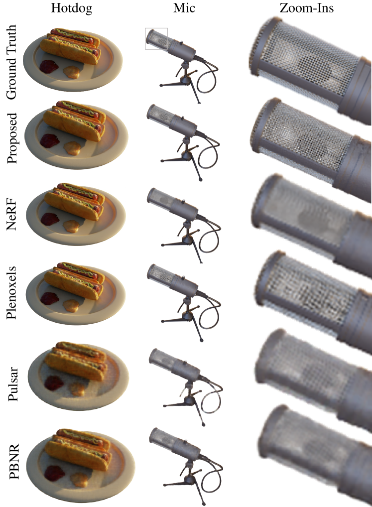
We test the proposed method on the rendered multi-view images from the Blender dataset used in NeRF [Mildenhall et al., 2020]. Note that this dataset provides background masks that are automatically extracted from the Z-buffer during rendering. We compare our method against state-of-the-art methods for novel-view synthesis: IBRNet [Wang et al., 2021], MVSNeRF [Chen et al., 2021b], Plenoxels [Yu et al., 2021a], Pulsar [Lassner and Zollhofer, 2021], and PBNR [Kopanas et al., 2021]. We note that PBNR requires pre-processed geometry information such as point clouds and point features retrieved from conventional SfM. In contrast, the proposed method is network-free and learns both point cloud positions and appearance, without the need for separate input geometry. Quantitatively, although the full version of Plenoxel (model size of 1.1GB) performs better in terms of reconstruction quality than ours, its smaller version Plenoxel_s (model size of 234MB) is 1.8dB worse than ours in PSNR, while our model size is only 9MB. Table 1 shows that the proposed method outperforms existing methods in training speed, inference speed, and model size while maintaining comparable image quality. Figure 3 provides visualizations of the rendered images which validate that the synthesized images are on par with state-of-the-art methods.

4.2. Video View Synthesis

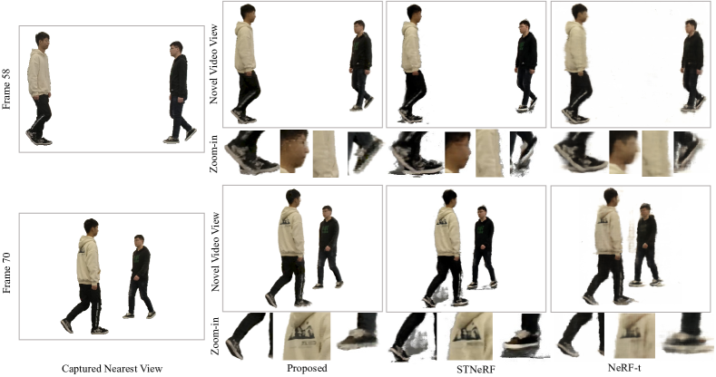
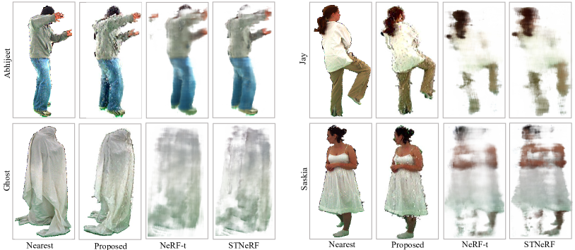
The computational efficiency and low memory footprint of the proposed point-based representation, allow it to explicitly represent challenging dynamic scenes better than implicit methods that rely on networks to produce time-conditional outputs as ST-NeRF and NeRF-T. Note that such NeRF-based per-frame modeling of videos results in a heavy computational load: for example, a 1000-frame video corresponding to a 40-seconds clip at 25FPS requires more than 20K GPU hours (per frame training) to train for a vanilla NeRF model and more than 1 terabyte storage (when trained per frame) for a Plenoxels [Yu et al., 2021a] model. Recently, Zhang et al. [2021] proposed NeRF-T and STNeRF as variants of NeRF that allow reducing the computational requirements of modeling videos for view synthesis by conditioning the radiance MLP of NeRF on the time $t$. While effective in reducing memory requirements, this comes at the cost of rendering quality compared to frame-by-frame modeling. The proposed method is light-weight and it allows for frame-by-frame learning with respect to both training time and storage. We evaluate the method on the video view synthesis datasets from STNeRF [Zhang et al., 2021] and the human motion dataset DSC [Vlasic et al., 2009]. Both of these two datasets contain background masks that are generated by a segmentation network and color thresholding, respectively. We note that the authors of STNeRF released only a portion of their entire dataset, which we use to perform our experiments. The dataset features 16 camera views distributed uniformly on a semicircle, from which we use 13 views for training and 3 views for testing. Table 2 and Figure 4 validate that our method outperforms the existing methods quantitatively and qualitatively. For experiments on DSC, please refer to the Appendix.

Table 2. Quantitative Evaluation on the STNeRF Dataset. Compared to STNeRF and the NeRF variants suggested in [Zhang et al., 2021], the training speed and inference speed of the proposed method is two orders of magnitude higher.

STNeRF	Train	Render	Model	Rendering Quality
				PSNR$\uparrow$	SSIM$\uparrow$	LPIPS$\downarrow$
NeRF	40 h	1/25 fps	14 MB	23.7 dB	0.853	0.304
NeRF-t	100 h	1/26 fps	16 MB	28.9 dB	0.913	0.259
STNeRF	50 h	1/30 fps	12 MB	32.1 dB	0.918	0.224
Ours	30 min	25 fps	110 MB	34.6 dB	0.927	0.207

4.3. Ablation Experiments

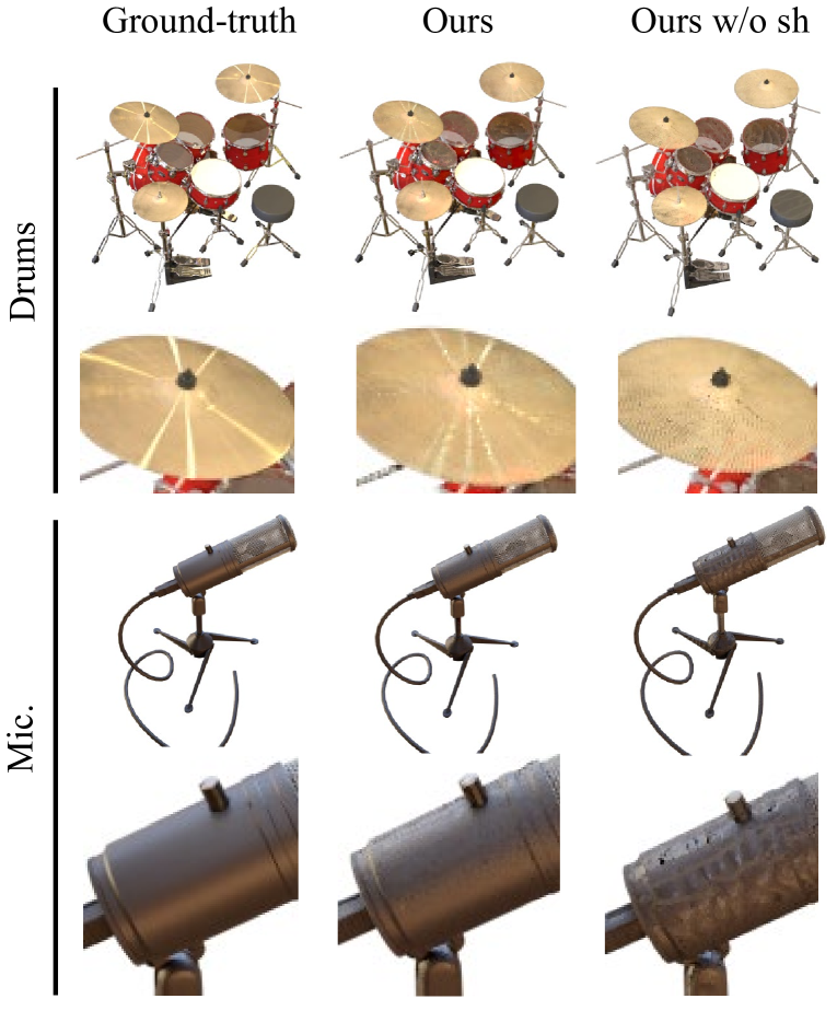
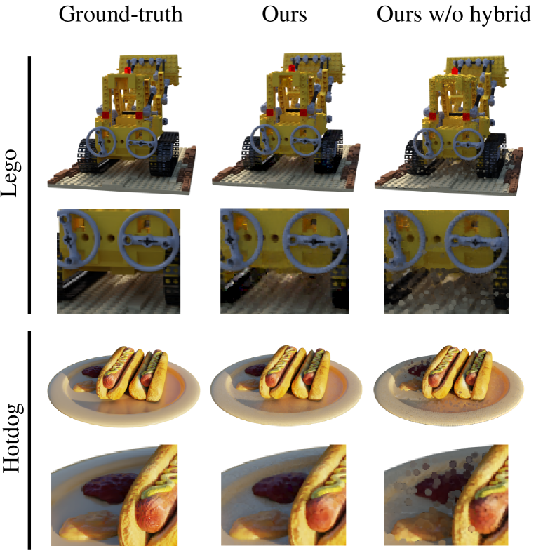
We evaluate each component of our method and validate their effectiveness. First, we replace the spherical harmonics with learnable directionally invariant RGB values denoted as “w/o sh”. Second, we remove the hybrid coarse-to-fine strategy and only train the point cloud in a single stage denoted as “w/o hybrid”. Third, we remove the consistency filter function (refer to the Appendix for additional details on initialization) for every epoch during training time, noted as ”w/o filter”. Table 3 shows that using spherical harmonics, the coarse-to-fine strategy, and the consistency filter function jointly achieves the best view synthesis performance. Please refer to the Appendix for corresponding qualitative results and additional ablation experiments.

Table 3. Model Ablation Experiments. We evaluate the rendering quality of our method on the Blender dataset [2020] when gradually removing components from the rendering pipeline. Specifically, we ablate the spherical harmonics model per point, the coarse-to-fine strategy, and the filtering function for the training. The experimental results validate that all components contribute to the rendering quality.

Module	Rendering Quality
	PSNR$\uparrow$	SSIM$\uparrow$	LPIPS$\downarrow$
w/o sh	27.1 dB	0.932	0.155
w/o hybrid	26.6 dB	0.925	0.163
w/o filter	29.1 dB	0.941	0.103
Ours	30.3 dB	0.945	0.078

5. Conclusion

Departing from volumetric representations of scene radiance, extensively explored in recent neural rendering work, we investigate an alternate radiance field representation that is based on points without giving up end-to-end differentiability. In contrast to coordinate-network representations that require ray-marching with hundreds of network evaluations per ray, the proposed representation allows us to render a novel view via differentiable splat-based rasterization. As a result, the proposed method is two orders of magnitude faster in training and inference time than volumetric methods, such as NeRF, while being on par in quality. The method does not require any pre-training and the representation is highly compact, occupying only 10 Mb per static scene. Future directions that may build on the approach introduced in this work could include hybrid point/surface models, or combine the proposed rendering method with point-based physical simulation methods.

Appendix

Additional Evaluations on the Synthetic Dataset

Tab.4 reports PSNR for every object for the static novel view synthesis experiment. Our method achieves quantitative results comparable to Plenoxels [Yu et al., 2021a] and NeRF [Mildenhall et al., 2020] while being resource-efficient in terms of memory and train/test runtime.

Table 4. Additional Static View Synthesis Evaluation. The proposed method achieves comparable performance to existing state-of-the-art view synthesis methods for static scenes while being more efficient in training/inference speed and memory usage.

	Chair	Drums	Ficus	Hotdog	Lego	Materials	Mic	Ship	Avg.
NeRF	33.00	25.01	30.13	36.18	32.54	29.62	32.91	28.65	31.01
Plenoxels	33.98	25.35	31.83	36.43	34.10	29.14	33.26	29.62	31.71
Ours	32.98	25.53	29.01	34.56	31.33	28.01	33.82	27.01	30.28

Discussion on the Usage of Background Masks

One limitation of our method is that it requires background masks to produce the initial point cloud. Although the improvements in training and testing time are not results of this initialization but the point cloud representation itself, it is an important step of the proposed approach. In our experiments, we consider datasets that provide the masks for single-object scenes, either generated by a separate segmentation network or extracted from the Z-Buffer for synthetic scenes. For more complex scenes which are more challenging to segment future work could extend the proposed method by relaxing the consistency check function to a soft check. Next, we discuss the usage of masks in the competing methods from Tab.4 above. Using masks in NeRF is investigated in VaxNeRF [2021]. In reconstruction quality, the proposed method fares on average 0.1 dB above the results of VaxNeRF. During inference, the proposed method (32 fps) is two orders of magnitude faster than VaxNeRF (0.1 fps). As such, the proposed model not only benefits from masks, but also from the representation and optimization method. To train a Plenoxel model, Yu et al. [2021a] require masks to determine the bounding volume to optimize for a Plenoxel model. Finally, we note that methods like Pulsar [2021] require more than just masks. Pulsar uses conventional SfM (COLMAP) to build a dense point cloud, which it then passes to SIBR to get a depth map and a normal map. We note that for single objects, a rich body of work has explored background extraction methods using such depth maps.

Figure 5. Ablating View Dependence. We visualize the ablations of the learnable spherical harmonics. For the mic object, we observe noticeable artifacts on the object surface if we remove the view-dependence module. This is due to the optimization with color inconsistency from different views.

Additional Visualization on the Blender Dataset

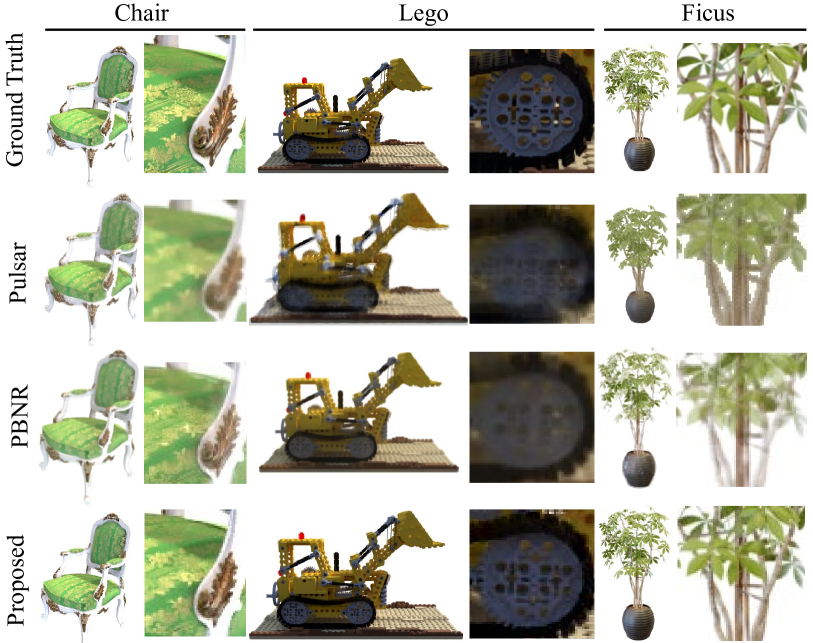
Fig.6 provides further visualizations for results on Blender dataset from [Mildenhall et al., 2020]. The proposed approach achieves substantially better rendering quality than the two recent point-based rendering baselines: Pulsar and PBNR.

Figure 6. Additional Comparison to Point-based Methods. We visualize novel views rendered for the Chair, Lego and Ficus objects from the Blender dataset from [Mildenhall et al., 2020], validating that our method outperforms existing point-based view synthesis methods.

Figure 7. View Ablations. We evaluate the quality of the proposed point-based method and the volumetric NeRF [2020] on the ’Ficus’ scene [2020] with a gradually reduced number of training views. The proposed sparse representation allows for reconstructions with reasonable quality even with as few as 20 views, where NeRF drops by more than 10 dB in PSNR.

Figure 8. Analysis of Coarse-to-Fine Optimization. We analyze rendering quality with and without the hybrid coarse-to-fine training strategy. We observe noticeable outlier points if we train the model without the coarse-to-fine training strategy, validating the proposed approach.

Figure 9. Novel View Synthesis on the DSC Dataset. We synthesize novel views for videos from the DSC dataset[2009] (frame 50 for every scene). We show the nearest captured frame on the left. We retrained STNeRF [2021] and the NeRF-t variant suggested by the authors on the same data. In contrast to the proposed method, these existing approaches fail in highly dynamic scenes (right).

Additional Ablation Studies

We evaluate the impact of the number of points on the final rendering quality to assess the trade-off between reconstruction accuracy and computational efficiency, reported Table 6. While a large number of points can better represent a scene radiance field, at the cost of higher computing and memory, diminishing returns can be observed at circa 50k points for the given static scenes we evaluate the method on.

We also assess the proposed method with and without modeling view dependence with spherical harmonics in Fig.5. Modeling view dependence is essential for the proposed model to represent specular highlights, as apparent on the brass symbols and the plastic surface on the microphone object. These experiments further validate the proposed model that relies on learnable spherical harmonics.

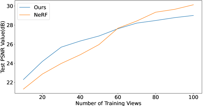
In Figure 7, we also provide an ablation study for sparse training views on the “Ficus” object from the Synthetic Blender dataset. Although our method performs slightly worse than the NeRF baseline when training on the whole 100 views, the method gradually improves on NeRF when the training images become sparser.

Additional Evaluations on the DSC Dataset

In the DSC dataset, 8 cameras are distributed in a 360^∘ setup and we use all of them to train the model (due to the overall low number of camera views). We argue that view synthesis on DSC is very challenging since there are only 8 training views available, covering 360 degrees, and with slight pose miscalibration. We report quantitative results in Table 5 and qualitative results in Figure 9 that further corroborate the findings we made for the STNeRF dataset. In all cases, the proposed method achieves high-quality view synthesis results with orders of magnitude decreased training time and improved inference speed.

Figure 10. Point Cloud Visualizations Evolving Throughout Training. As training progresses, the learned point cloud approximates the object geometry more accurately, illustrating the effectiveness of the positional updates of the proposed optimization method.

Table 5. Quantitative Evaluation on the DSC Dataset. We report the training time, rendering speed and the model size required to represent scenes from the DSC[Vlasic et al., 2009] dataset with the proposed method. Note that we train a radiance point cloud for each frame here and we report the total memory consumption.

STNeRF	Train	Render	Model
NeRF	50 h	1/15 fps	14 MB
NeRF-t	75 h	1/15 fps	16 MB
STNeRF	86 h	1/18 fps	12 MB
Ours	1 h	28 fps	240 MB

Table 6. Point Cloud Size Ablations. The rendering quality of the proposed method grows with the density of the point cloud (for a given volume), at the cost of training time, inference speed and model size. We trade off these dimensions and choose 45k points for our experiments.

. Point Scale Train Render Model PSNR$\uparrow$ 15 k 16 min 35 fps 37 MB 32.2 dB 30 k 20 min 32 fps 73 MB 33.6 dB 45 k 30 min 25 fps 110 MB 34.6 dB 60 k 41 min 16 fps 146 MB 34.8 dB 100 k 76 min 10 fps 244 MB 34.2 dB

Additional Initialization Details

Next, we provide further details on the point cloud initialization from initial image masks. We first uniformly sample points from scene volume. For each 3D point $P^{j}$, we compute the projected 2D point $p_{i}^{j}$ on a camera $i$ using Eq.1. After each projection, we check whether the corresponding pixel is a background pixel, in which case we discard the point. Specifically, we define the following consistency check function

$$\mathcal{CC}(p^{j})=\mathbb{I}(\sum_{i=1}^{N}\mathbb{I}(M_{i}(p_{i}^{j})>0)=N),$$

where $M_{i}(\cdot)$ is the foreground mask and $\mathbb{I}(\cdot)$ is the indicator function. We compute the value of this consistency function for every sample point and only keep the point if the value is true. We also use this consistency function during the training time by filtering out points that become inconsistent after every training epoch.

Algorithm 1 Hybrid Coarse-to-Fine Update Strategy

0:  Coarse point cloud $S=\{P_{i}|P_{i}=(x_{i},y_{i},z_{i},f_{i})\}$,

0:  Hyper-parameters $N,K,\epsilon$

0:  New point cloud $S^{{}^{\prime}}=\{P_{i}|P_{i}=(x_{i},y_{i},z_{i},f_{i})\}$

1:  $S^{{}^{\prime}}=\emptyset$,  Partition the space into $N\times N\times N$ voxels.

2:  for each voxel do

3:     Fetch all the points $\{P_{1},P_{2},...,P_{M}\}$ inside this voxel.

4:     Compute the average: $P_{a}=\frac{1}{M}\sum\limits_{i=1}^{M}$.

5:     Add $P_{a}$ to $S^{{}^{\prime}}$.

6:  end for

7:  for $P_{i}\in S^{{}^{\prime}}$ do

8:     Fetch neighbor $K$ points $\{P_{1},P_{2},...,P_{K}\}$ for $P_{i}$.

9:     Compute distances between neighbors and $P_{i}$ to get $\{d_{1},d_{2},...,d_{K}\}$

10:     Compute standard deviation $\delta$ for set $\{d_{1},d_{2},...,d_{K}\}$

11:     if $\delta>\epsilon$ then

12:        Remove $P_{i}$ from $S^{{}^{\prime}}$

13:     end if

14:  end for

15:  for $P_{i}\in S^{{}^{\prime}}$ do

16:     Fetch neighbor $K$ points $\{P_{1},P_{2},...,P_{K}\}$ for $P_{i}$.

17:     Compute the average: $P_{a}=\frac{1}{K}\sum\limits_{i=1}^{K}P_{i}$.

18:     Add $P_{a}$ to $S^{{}^{\prime}}$.

19:  end for

20:  return  $S^{{}^{\prime}}$

Additional Algorithm Details

To supplement the description in the main text, Algorithm 1 contains pseudo-code of our coarse-to-fine update method. We further note that all code, models and data required to reproduce the findings in this work have been published.

Point Cloud Evolution During Training

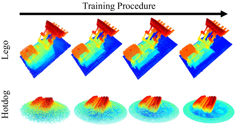
We visualize the evolution of the learned point clouds during training in Fig.10. As the training progresses, we can observe three trends: the point cloud approximates the target geometry more accurately with more training, the outliers are eliminated with additional training stages, and the concave regions are progressively improved with additional training iterations. These additional visualization qualitatively validate the proposed training scheme.

References

- [1]
- Aliev et al. [2020] Kara-Ali Aliev, Artem Sevastopolsky, Maria Kolos, Dmitry Ulyanov, and Victor Lempitsky. 2020. Neural point-based graphics. In European Conference on Computer Vision. Springer, 696–712.
- Basri and Jacobs [2003] Ronen Basri and David W. Jacobs. 2003. Lambertian Reflectance and Linear Subspaces. IEEE Trans. PAMI 25, 2 (2003), 218–233.
- Cabral et al. [1987] Brian Cabral, Nelson Max, and Rebecca Springmeyer. 1987. Bidirectional Reflection Functions from Surface Bump Maps. Computer Graphics (Proc. SIGGRAPH) 21, 4 (1987), 273–281.
- Chen et al. [2021b] Anpei Chen, Zexiang Xu, Fuqiang Zhao, Xiaoshuai Zhang, Fanbo Xiang, Jingyi Yu, and Hao Su. 2021b. MVSNeRF: Fast Generalizable Radiance Field Reconstruction from Multi-View Stereo. In Proc. ICCV.
- Chen et al. [2021a] Zhe Chen, Shohei Nobuhara, and Ko Nishino. 2021a. Invertible Neural BRDF for Object Inverse Rendering. IEEE Trans. PAMI (2021).
- Furukawa and Ponce [2009] Yasutaka Furukawa and Jean Ponce. 2009. Accurate, Dense, and Robust Multiview Stereopsis. IEEE Trans. PAMI 32, 8 (2009), 1362–1376.
- Garbin et al. [2021] Stephan J Garbin, Marek Kowalski, Matthew Johnson, Jamie Shotton, and Julien Valentin. 2021. FastNeRF: High-Fidelity Neural Rendering at 200FPS. In Proc. ICCV.
- Han et al. [2020] Zhizhong Han, Chao Chen, Yu-Shen Liu, and Matthias Zwicker. 2020. DRWR: A Differentiable Renderer without Rendering for Unsupervised 3D Structure Learning from Silhouette Images. In Proc. ICML.
- Hedman et al. [2021] Peter Hedman, Pratul P Srinivasan, Ben Mildenhall, Jonathan T Barron, and Paul Debevec. 2021. Baking neural radiance fields for real-time view synthesis. In Proceedings of the IEEE/CVF International Conference on Computer Vision. 5875–5884.
- Im et al. [2019] Sunghoon Im, Hae-Gon Jeon, Stephen Lin, and In So Kweon. 2019. DPSNet: End-to-end Deep Plane Sweep Stereo. In Proc. ICLR.
- Kondo et al. [2021] Naruya Kondo, Yuya Ikeda, Andrea Tagliasacchi, Yutaka Matsuo, Yoichi Ochiai, and Shixiang Shane Gu. 2021. Vaxnerf: Revisiting the classic for voxel-accelerated neural radiance field. arXiv preprint arXiv:2111.13112 (2021).
- Kopanas et al. [2021] Georgios Kopanas, Julien Philip, Thomas Leimkühler, and George Drettakis. 2021. Point-Based Neural Rendering with Per-View Optimization. In Computer Graphics Forum, Vol. 40. Wiley Online Library, 29–43.
- Lassner and Zollhofer [2021] Christoph Lassner and Michael Zollhofer. 2021. Pulsar: Efficient sphere-based neural rendering. In Proceedings of the IEEE/CVF Conference on Computer Vision and Pattern Recognition. 1440–1449.
- Liu et al. [2021] Yuan Liu, Sida Peng, Lingjie Liu, Qianqian Wang, Peng Wang, Christian Theobalt, Xiaowei Zhou, and Wenping Wang. 2021. Neural Rays for Occlusion-aware Image-based Rendering. arXiv:2107.13421.
- Lombardi et al. [2019] Stephen Lombardi, Tomas Simon, Jason Saragih, Gabriel Schwartz, Andreas Lehrmann, and Yaser Sheikh. 2019. Neural Volumes: Learning Dynamic Renderable Volumes from Images. ACM Trans. Graphics 38, 4, Article 65 (July 2019).
- Lombardi et al. [2021] Stephen Lombardi, Tomas Simon, Gabriel Schwartz, Michael Zollhoefer, Yaser Sheikh, and Jason Saragih. 2021. Mixture of volumetric primitives for efficient neural rendering. ACM Transactions on Graphics (TOG) 40, 4 (2021), 1–13.
- Marroquim et al. [2007] Ricardo Marroquim, Martin Kraus, and Paulo Roma Cavalcanti. 2007. Efficient Point-Based Rendering Using Image Reconstruction. In Proc. PBG. 101–108.
- Meshry et al. [2019] Moustafa Meshry, Dan B Goldman, Sameh Khamis, Hugues Hoppe, Rohit Pandey, Noah Snavely, and Ricardo Martin-Brualla. 2019. Neural Rerendering in the Wild. In Proc. CVPR. 6878–6887.
- Mildenhall et al. [2020] Ben Mildenhall, Pratul P Srinivasan, Matthew Tancik, Jonathan T Barron, Ravi Ramamoorthi, and Ren Ng. 2020. NeRF: Representing Scenes as Neural Radiance Fields for View Synthesis. In Proc. ECCV. Springer, 405–421.
- Neff et al. [2021] Thomas Neff, Pascal Stadlbauer, Mathias Parger, Andreas Kurz, Joerg H Mueller, Chakravarty R Alla Chaitanya, Anton Kaplanyan, and Markus Steinberger. 2021. DONeRF: Towards Real-Time Rendering of Compact Neural Radiance Fields using Depth Oracle Networks. In Computer Graphics Forum, Vol. 40. Wiley Online Library, 45–59.
- Pfister et al. [2000] Hanspeter Pfister, Matthias Zwicker, Jeroen Van Baar, and Markus Gross. 2000. Surfels: Surface Elements as Rendering Primitives. In Computer Graphics (Proc. SIGGRAPH). 335–342.
- Ramamoorthi and Hanrahan [2001a] Ravi Ramamoorthi and Pat Hanrahan. 2001a. An Efficient Representation for Irradiance Environment Maps. In Computer Graphics (Proc. SIGGRAPH). 497–500.
- Ramamoorthi and Hanrahan [2001b] Ravi Ramamoorthi and Pat Hanrahan. 2001b. On the Relationship Between Radiance and Irradiance: Determining the Illumination from Images of a Convex Lambertian Object. JOSA A 18, 10 (2001), 2448–2459.
- Reiser et al. [2021] Christian Reiser, Songyou Peng, Yiyi Liao, and Andreas Geiger. 2021. KiloNeRF: Speeding up Neural Radiance Fields with Thousands of Tiny MLPs. arXiv:2103.13744.
- Rosenthal and Linsen [2008] Paul Rosenthal and Lars Linsen. 2008. Image-space Point Cloud Rendering. In Proc. CGI. 136–143.
- Rückert et al. [2021] Darius Rückert, Linus Franke, and Marc Stamminger. 2021. ADOP: Approximate Differentiable One-Pixel Point Rendering. arXiv:2110.06635.
- Schönberger et al. [2016] Johannes L Schönberger, Enliang Zheng, Jan-Michael Frahm, and Marc Pollefeys. 2016. Pixelwise View Selection for Unstructured Multi-View Stereo. In Proc. ECCV. Springer, 501–518.
- Sillion et al. [1991] Françis X Sillion, James R Arvo, Stephen H Westin, and Donald P Greenberg. 1991. A Global Illumination Solution for General Reflectance Distributions. In Computer Graphics (Proc. SIGGRAPH). 187–196.
- Sloan et al. [2003] Peter-Pike Sloan, Jesse Hall, John Hart, and John Snyder. 2003. Clustered Principal Components for Precomputed Radiance Transfer. ACM Trans. Graphics 22, 3 (2003), 382–391.
- Sloan et al. [2002] Peter-Pike Sloan, Jan Kautz, and John Snyder. 2002. Precomputed Radiance Transfer for Real-Time Rendering in Dynamic, Low-Frequency Lighting Environments. In Computer Graphics (Proc. SIGGRAPH). 527–536.
- Sztrajman et al. [2021] Alejandro Sztrajman, Gilles Rainer, Tobias Ritschel, and Tim Weyrich. 2021. Neural BRDF Representation and Importance Sampling. Computer Graphics Forum 40, 6 (2021), 332–346.
- Thonat et al. [2021] Théo Thonat, Yagiz Aksoy, Miika Aittala, Sylvain Paris, Frédo Durand, and George Drettakis. 2021. Video-Based Rendering of Dynamic Stationary Environments from Unsynchronized Inputs. In Computer Graphics Forum, Vol. 40. Wiley Online Library, 73–86.
- Vlasic et al. [2009] Daniel Vlasic, Pieter Peers, Ilya Baran, Paul Debevec, Jovan Popović, Szymon Rusinkiewicz, and Wojciech Matusik. 2009. Dynamic Shape Capture using Multi-View Photometric Stereo. ACM Trans. Graphics 28, 5 (Dec. 2009).
- Wang et al. [2021] Qianqian Wang, Zhicheng Wang, Kyle Genova, Pratul Srinivasan, Howard Zhou, Jonathan T. Barron, Ricardo Martin-Brualla, Noah Snavely, and Thomas Funkhouser. 2021. IBRNet: Learning Multi-View Image-Based Rendering. In Proc. CVPR.
- Wiles et al. [2020] Olivia Wiles, Georgia Gkioxari, Richard Szeliski, and Justin Johnson. 2020. Synsin: End-to-end view synthesis from a single image. In Proceedings of the IEEE/CVF Conference on Computer Vision and Pattern Recognition. 7467–7477.
- Wizadwongsa et al. [2021] Suttisak Wizadwongsa, Pakkapon Phongthawee, Jiraphon Yenphraphai, and Supasorn Suwajanakorn. 2021. NeX: Real-time View Synthesis with Neural Basis Expansion. In Proc. CVPR.
- Wood et al. [2000] Daniel N Wood, Daniel I Azuma, Ken Aldinger, Brian Curless, Tom Duchamp, David H Salesin, and Werner Stuetzle. 2000. Surface Light Fields for 3D Photography. In Computer Graphics (Proc. SIGGRAPH). 287–296.
- Xu et al. [2022] Qiangeng Xu, Zexiang Xu, Julien Philip, Sai Bi, Zhixin Shu, Kalyan Sunkavalli, and Ulrich Neumann. 2022. Point-nerf: Point-based neural radiance fields. In Proceedings of the IEEE/CVF Conference on Computer Vision and Pattern Recognition. 5438–5448.
- Yao et al. [2018] Yao Yao, Zixin Luo, Shiwei Li, Tian Fang, and Long Quan. 2018. MVSNet: Depth Inference for Unstructured Multi-view Stereo. In Proc. ECCV. 767–783.
- Yifan et al. [2019] Wang Yifan, Felice Serena, Shihao Wu, Cengiz Öztireli, and Olga Sorkine-Hornung. 2019. Differentiable Surface Splatting for Point-based Geometry Processing. ACM Trans. Graphics 38, 6 (2019), 1–14.
- Yu et al. [2021a] Alex Yu, Sara Fridovich-Keil, Matthew Tancik, Qinhong Chen, Benjamin Recht, and Angjoo Kanazawa. 2021a. Plenoxels: Radiance Fields without Neural Networks. arXiv:2112.05131.
- Yu et al. [2021b] Alex Yu, Ruilong Li, Matthew Tancik, Hao Li, Ren Ng, and Angjoo Kanazawa. 2021b. PlenOctrees for Real-time Rendering of Neural Radiance Fields. In Proc. ICCV.
- Yu et al. [2021c] Alex Yu, Vickie Ye, Matthew Tancik, and Angjoo Kanazawa. 2021c. pixelNeRF: Neural Radiance Fields from One or Few Images. In Proc. CVPR. 4578–4587.
- Zhang et al. [2021] Jiakai Zhang, Xinhang Liu, Xinyi Ye, Fuqiang Zhao, Yanshun Zhang, Minye Wu, Yingliang Zhang, Lan Xu, and Jingyi Yu. 2021. Editable Free-Viewpoint Video using a Layered Neural Representation. ACM Trans. Graphics 40, 4 (2021), 1–18.
- Zhou et al. [2018] Tinghui Zhou, Richard Tucker, John Flynn, Graham Fyffe, and Noah Snavely. 2018. Stereo Magnification: Learning View Synthesis using Multiplane Images. ACM Trans. Graphics 37, 4, Article 65 (Aug. 2018).
- Zwicker et al. [2002] Matthias Zwicker, Mark Pauly, Oliver Knoll, and Markus Gross. 2002. Pointshop 3D: An Interactive System for Point-Based Surface Editing. ACM Trans. Graphics 21, 3 (2002), 322–329.
- Zwicker et al. [2001] Matthias Zwicker, Hanspeter Pfister, Jeroen Van Baar, and Markus Gross. 2001. Surface Splatting. In Computer Graphics (Proc. SIGGRAPH). 371–378.
- Zwicker et al. [2004] Matthias Zwicker, Jussi Räsänen, Mario Botsch, Carsten Dachsbacher, and Mark Pauly. 2004. Perspective Accurate Splatting. In Proc. Graphics Interface. 247–254.