Triple-Band Scheduling with Millimeter Wave and Terahertz Bands for Wireless Backhaul

Abstract

With the explosive growth of mobile traffic demand, densely deployed small cells underlying macrocells have great potential for 5G and beyond wireless networks. In this paper, we consider the problem of supporting traffic flows with diverse QoS requirements by exploiting three high frequency bands, i.e., the 28GHz band, the E-band, and the Terahertz (THz) band. The cooperation of the three bands is helpful for maximizing the number of flows with their QoS requirements satisfied. To solve the formulated nonlinear integer programming problem, we propose a triple-band scheduling scheme which can select the optimum scheduling band for each flow among three different frequency bands. The proposed scheme also efficiently utilizes the resource to schedule flow transmissions in time slots. Extensive simulations demonstrate the superior performance of the proposed scheme over three baseline schemes with respect to the number of completed flows and the system throughput.

I Introduction

Over the last few years, the explosive growth of mobile data demand has always been the focus of attention. Edholm’s law reveals that wireless data rates have doubled every 18 months. Moreover, the world monthly mobile traffic will be about 49 exabytes by the year 2021 [1]. It is apparent that the existing communication technologies and the available spectrum resources cannot fully support such huge data demand. Therefore, many solutions have been proposed to deal with the problem of excessive data demand. Among the many potential solutions, densely deployed small cells underlying macrocells are shown effective on achieving higher network capacity [2, 3]. Traffic offloading with small cells can effectively ease the burden on macrocells [4]. The short transmission range in small cells enhances the transmission quality and leads to higher transmission rates. Although various technologies (such as modulation, multiplexing, multiple antennas, etc.) have been used to deal with the massive traffic demands, the communications in higher frequency bands (i.e., spectrum expansion) seems to be the most effective means to deal with the ever-increasing rate demands [5]. To this end, millimeter-wave (mmWave) communications have been proposed as a key component of 5G wireless networks [6]. However, substantial studies have shown the limits of the current wireless networks that rely on the mmWave frequency bands. In order to obtain greater transmission bandwidth, Terahertz (THz) band should be utilized to even further increase the achievable rates of the 5G beyond wireless networks. For wireless communications in the THz band, apart from issues of electronics (such as the design of high power compact transceivers [7]), the very high free-space attenuation by spreading loss is also a big challenge.

In fact, behind the explosive growth of data demand is a large number of existing and emerging applications. The transmission rate requirements of different applications are highly diverse. For example, web browsing usually only requires a multi-Mbps transmission rate, but streaming an uncompressed high-definition TV (HDTV) requires a multi-Gbps rate [8, 9, 10]. Although the single high frequency band with enough bandwidth may be used for the scheduling of a large number of different flows, the advantages would be obvious if multiple bands can be utilized to schedule the diverse traffic flows. According to the transmission characteristics of different frequency bands, choosing the appropriate band for different flow transmissions is conducive to improving the system performance.

In this paper, we consider the backhaul network with densely deployed small cells underlying a macrocell. There are a set of flows to be scheduled with their minimum throughput requirements (i.e., the lowest transmission rate requirements), which are also referred to as the quality of service (QoS) requirements in this paper. QoS requirements of different flows are highly diverse. We propose to exploit two mmWave bands (including one lower frequency mmWave band and the E-band) and one THz band to carry these flows. The proposed band selection algorithm determines the transmission band of each flow based on its QoS requirement and transmission range. Moreover, we propose a triple-band scheduling algorithm to schedule transmissions of the flows in different bands and time slots. The contributions of this paper can be summarized as follows.

• To fully exploit the available spectrum resources, we propose the cooperation of three bands (i.e., two mmWave bands and one THz band) to schedule a large number of flows with diverse QoS requirements. In order to avoid the pressure putting all flows in the highest frequency band, we disperse flows with relatively lower QoS requirements to the lower frequency band for transmission. This approach allows more resources for other flows with more stringent QoS requirements.

• We formulate the problem of optimal triple-band scheduling as a nonlinear integer programming problem. Moreover, we propose a heuristic triple-band scheduling algorithm to maximize the number of flows with their QoS requirements satisfied within a fixed time. The algorithm determines whether flows conflict with each other based on their mutual interference.

• We evaluate the proposed triple-band scheduling scheme for the backhaul network in the 28GHz, 73GHz, and 340GHz bands with extensive simulations. The simulation results demonstrate that our proposed scheme outperforms three baseline schemes on both the number of completed flows and the system throughput.

The remainder of this paper is organized as follows. Section II reviews the related work. Section III introduces the system model. In Section IV, we formulate the optimal triple-band scheduling problem as a nonlinear integer programming problem. In Section V, we propose the triple-band scheduling scheme with the transmission band selection algorithm. In Section VI, we evaluate the proposed scheme with simulations. Section VII concludes this paper.

II Related Work

There are many studies on flow scheduling in mmWave networks with a single frequency band. In [11], a scheduling scheme based on time division multiple access (TDMA) is proposed to support the communications from one point to multiple points in mmWave backhaul networks. In [12], the authors design a scheduling algorithm for backhaul networks by exploiting mmWave macro base stations as relay nodes. In [13], an efficient polynomial-time scheduling method and an approximation algorithm parallel data stream scheduling method are proposed for no interference network model. In [14], the authors optimize the scheduling of access and backhaul links to maximize the achievable minimum throughput of the access links. In [15], an algorithm is proposed to find high throughput paths with relays for links by minimizing interference within and between paths. In [16], a relay selection algorithm and a transmission scheduling algorithm are proposed to relay the blocked flows and maximize the number of completed flows. In this paper, we consider the transmissions in the THz band in addition to the mmWave band, and aim to maximize the number of scheduling flows.

In addition, there are also some related works on communications in the THz band. In [17], the authors propose an approach to enhance the performance of cellular networks with THz links. In [18], the authors propose an algorithm of QoS-aware bandwidth allocation and concurrent scheduling. In [19], a sub-channel allocation method and power allocation scheme based on improved Whale Optimization Algorithm is proposed. Furthermore, multi-band cooperation has also been applied in a few areas. In [1], a control-data separation architecture for dual-band mmWave networks is proposed. In [20], a wireless local area network (WLAN) architecture utilizing the new multi-beam transmissions in sub-6GHz and mmWave dual-band cooperation mechanisms is proposed to improve the throughput and reliability of the network. This paper variously seeks a mode of cooperation in mmWave and THz band, instead of only focusing on mmWave communication or THz communication as the works listed above.

However, these existing related works have not considered the case of a triple-band cooperation involving both mmWave and THz communications. To the best of our knowledge, there is no research on a scheduling problem that incorporates multi-band transmissions. This is mainly due to the complexity of THz transmission itself and the high cost of transmission equipment. In this paper, through the integration of multi-band cooperation into the scheduling problem, we will show that the performance with respect to the number of completed flows and the system throughput could be greatly improved.

III System Overview

TABLE I: Summary of Notation and Description

Notation	Description
$M$, $\Delta t$, $t_{0}$	number of TSs, time duration of the TS, time duration of the scheduling phase
${P_{r}^{mmWave}}(i,i)$, ${P_{r}^{THz}}(i^{\prime},i^{\prime})$	received power of flow $i$ in mmWave band (28GHz band or E-band), received power of flow $i^{\prime}$ in THz band
$P_{t}^{mmWave}$, $P_{t}^{THz}$	transmit power of mmWave transmission (28GHz transmission or E-band transmission), transmit power of THz transmission
$G^{t}_{s_{i}}$, $G^{r}_{r_{i}}$	directional antenna gain at transmitter $s_{i}$, directional antenna gain at receiver $r_{i}$
$d_{s_{i}r_{i}}$	distance between $t_{i}$ and $r_{i}$
$f^{THz}$	carrier frequency of THz band
$\lambda^{mmWave}$, $\lambda^{THz}$	wavelength of mmWave band (28GHz band or E-band), wavelength of THz band
$k_{0}^{mmWave}$	free space path loss of mmWave transmission
${I_{ji}^{mmWave}}$, ${I_{{j^{\prime}}{i^{\prime}}}^{THz}}$	interference at $r_{i}$ from $s_{j}$ in mmWave band, interference at $r^{\prime}_{i}$ from $s^{\prime}_{j}$ in THz band
${l^{THz}}(i^{\prime},i^{\prime})$	path loss of the flow $i^{\prime}$ in THz band
$R_{i}^{mmWave}$, $W_{i}^{mmWave}$	transmission rate of flow $i$ in mmWave band (28GHz band or E-band), bandwidth of mmWave band (28GHz band or E-band)
$W^{mm}$, $W^{me}$, $W^{THz}$	bandwidth of 28GHz band, bandwidth of E-band, bandwidth of THz band
$N_{0}^{THz}(i^{\prime})$	total noise at the receiver of flow $i^{\prime}$ in THz band
$R_{i}^{mm}$, $R_{i}^{me}$, $R_{i}^{THz}$	transmission rate of flow $i$ in 28GHz band, transmission rate of flow $i$ in E-band, transmission rate of flow $i$ in THz band
$\theta^{t}_{ml}$, $\theta^{r}_{ml}$	beamwidth of the main lobe of transmitter antenna, beamwidth of the main lobe of receiver antenna
$q_{i}$, $T_{i}$	QoS requirement of flow $i$, actual throughput of flow $i$
$D_{ref}^{THz}$	reference distance of THz communication
$\delta$	type of bands ($\delta=mm$ is 28GHz band, $\delta=me$ is E-band or $\delta=THz$ is THz band)
$Q_{i}$	binary variable of flow state ($Q_{i}=0$ indicates flow $i$ is uncompleted or $Q_{i}=1$ indicates flow $i$ is completed)
$a_{i_{mm}}^{t}$, $a_{i_{me}}^{t}$, $a_{i_{T}}^{t}$	binary variable of flow state in 28GHz band in TS $t$ ($a_{i_{mm}}^{t}=0$ indicates flow $i$ isn’t scheduled in 28GHz band in TS $t$ or $a_{i_{mm}}^{t}=1$ indicates flow $i$ is scheduled in 28GHz band in TS $t$ ), binary variable of flow state in E-band in TS $t$, binary variable of flow state in THz band in TS $t$

In this paper, we consider a backhaul network supporting densely deployed small cells, as shown in Fig. 1. The backhaul network controller (BNC) resides on one of the gateways to synchronize the network, receive the QoS requirements of different flows, and obtain the BS locations. Each BS is equipped with an electronically steerable directional antenna which can transmit in narrow beams towards other BSs, and operate in the half duplex (HD) mode. If there is a certain amount of traffic demand between any two BSs, a flow is requested between the pair of BSs. Each flow has its minimum throughput requirement, which is the QoS requirement of the flow considered in this paper. To serve a large amount of traffic demand with a wide range of QoS requirements, we adopt a triple-band transmission approach that utilizing the 28GHz band, the E-band, and the THz band. Compared with the mmWave band, the THz band has much more bandwidth available, but its higher propagation loss results in shorter transmission ranges. It is an interesting problem to investigate how to schedule the flows over the multiple bands to maximizing the throughput of the network.

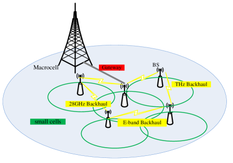
Figure 1: The backhaul network in the small cells densely deployed scenario.

III-A System Model

Since non-line-of-sight (NLOS) transmissions suffer from much higher attenuation than line-of-sight (LOS) transmissions in both mmWave and THz bands [21], we assume there is a directional LOS link between any pair of BSs by appropriate adjusting the locations of the BSs. In the heterogeneous network, there are $N$ BSs and $F$ flows which need to be transmitted among the $N$ BSs. The flows can transmit in either one of the mmWave bands or the THz band in this paper. Therefore, we need to consider the transmission models of a flow in different bands.

In the system, time is divided into a series of non-overlapping superframes, and each superframe consists of a scheduling phase and a transmission phase. The scheduling phase is the time duration to collect flow requests and their QoS requirements. The transmission phase consists of $M$ equal time slots (TSs). For clarity of illustration, we use TSs to measure the transmission time. For reliable transmission, the control signaling and BS requests can be collected by the BSs using 4G transmissions, when the BNC receives the source/destination BSs information and QoS requirements for each flow [22] (assuming the BS locations are already known, since they are fixed). The proposed scheduler is to allow multiple flows be transmitted concurrently using the spatial-time division multiple access (STDMA) in this paper [23].

III-A1 mmWave Transmission Model

For a flow $i$ that is transmitted from transmitter $s_{i}$ in the 28GHz band or E-band, the received power at its receiver $r_{i}$ can be calculated as

$${P_{r}^{mmWave}}(i,i)={k_{0}^{mmWave}}G^{t}_{s_{i}}G^{r}_{r_{i}}d_{s_{i}r_{i}}^{-n}{P_{t}^{mmWave}},$$ (1)

where $k_{0}^{mmWave}$ is the free space path loss of mmWave transmission at the reference distance 1m, which is proportional to $\left(\frac{\lambda^{mmWave}}{{4\pi}}\right)^{2}$, where $\lambda^{mmWave}$ is the wavelength and $P_{t}^{mmWave}$ is the transmit power of the mmWave transmission [24]; $G^{t}_{s_{i}}$ and $G^{r}_{r_{i}}$ are the directional antenna gain at $s_{i}$ and $r_{i}$, respectively; $d_{s_{i}r_{i}}$ denotes the distance between $t_{i}$ and $r_{i}$; and $n$ is the path loss exponent. Since the BSs operate in the HD mode, adjacent co-band flows that involve the same BS cannot be scheduled to transmit concurrently. For co-band flows $i$ and $j$ that do not involve the same BS, the interference at $r_{i}$ from $s_{j}$ can be calculated as

$${I_{ji}^{mmWave}}=\rho{k_{0}^{mmWave}}G^{t}_{s_{j}}G^{r}_{r_{i}}d_{s_{j}r_{i}}^{-n}{P_{t}^{mmWave}},$$ (2)

where $\rho$ is the factor of multi-user interference (MUI) that is related to the cross correlation of signals from different flows [25].

The transmission rate of flow $i$ can be obtained according to Shannon’s channel capacity, given by

$$R_{i}^{mmWave}=$$ (3)

$$\eta W_{i}^{mmWave}{\rm{log}}_{2}\left(1+\frac{{P_{r}^{mmWave}}(i,i)}{N_{0}W_{i}^{mmWave}+\sum\limits_{j}I_{ji}^{mmWave}}\right),$$

where $\eta$ is in the range of $(0,1)$ and describes the efficiency of the transceiver design. $W_{i}^{mmWave}$ is the transmission bandwidth of the flow $i$, and $N_{0}$ is the onesided power spectra density of white Gaussian noise [26].

III-A2 THz Transmission Model

In the case that flow $i^{\prime}$ is transmitted in the THz band, the path loss is given by

$${l^{THz}}(i^{\prime},i^{\prime})=92.4+20lg(f^{THz})+20lg(d_{s_{i^{\prime}}r_{i^{\prime}}}),$$ (4)

the path loss model is proposed in Ref. [27], and is related to the frequency and distance of the transmission [28, 29]. The unit of $f^{THz}$ is $GHz$, and the unit of $d_{s_{i^{\prime}}r_{i^{\prime}}}$ is $km$. For the main molecule of the atmosphere, i.e., water-based absorption, the attenuation of some high THz bands can be as high as hundreds dB/km, and the attenuation of some lower spectrum THz bands is only few dB/km.

For flow $i^{\prime}$, the received power at its receiver $r_{i^{\prime}}$ from its transmitter $t_{i^{\prime}}$ can be calculated as

$${P_{r}^{THz}}(i^{\prime},i^{\prime})={l^{THz}}(i^{\prime},i^{\prime})G^{t}_{s_{i^{\prime}}}G^{r}_{r_{i^{\prime}}}{P_{t}^{THz}},$$ (5)

where $P_{t}^{THz}$ is the transmit power of the THz transmissions.

Similar to the mmWave case, we also consider the interference between co-band concurrent flows that do not involve the same BS (i.e., non-adjacent) in the THz band. For flows $i^{\prime}$ and $j^{\prime}$ in THz band, which are non-adjacent, the interference at $r_{i^{\prime}}$ from $s_{j^{\prime}}$ can be calculated as

$${I_{{j^{\prime}}{i^{\prime}}}^{THz}}=\rho^{\prime}{l^{THz}}(j^{\prime},i^{\prime})G^{t}_{s_{j^{\prime}}}G^{r}_{r_{i^{\prime}}}{P_{t}^{THz}},$$ (6)

where $\rho^{\prime}$ is the factor of multi-user interference (MUI), as the $\rho$ in (2). ${l^{THz}}(j^{\prime},i^{\prime})$ is the path loss of the flow from $s_{j^{\prime}}$ to $r_{i^{\prime}}$ in the THz band, which is calculated as (4).

Hence, according to Shannon’s channel capacity, the transmission rate of flow $i^{\prime}$ can be calculated as

$$R_{i^{\prime}}^{THz}=\eta W^{THz}{\rm{log}}_{2}\left(1+\frac{{P_{r}^{THz}}(i^{\prime},i^{\prime})}{N_{0}W^{THz}+\sum\limits_{j^{\prime}}I_{j^{\prime}i^{\prime}}^{THz}}\right),$$ (7)

where $W^{THz}$ is the bandwidth of the THz band.

There is a tradeoff in the choice of the carrier-frequency of the THz transmission, $f^{THz}$, which affects both the bandwidth and the path loss of the THz transmission. The higher the bandwidth that can be utilized, the higher the molecular absorption [28]. In this paper, we choose $f_{THz}=340$ GHz. Experiments show that the group velocity dispersion of the channel in this frequency band is very small, and the signal is not easy to be broadened. The maximum transmission rate of this frequency band can achieve more than 10 Gbps [27].

The output power of the THz amplifier is closely related to the electronic-circuit design and is limited by the current hardware technology. For instance, the carrier frequency of 340GHz is adopted in this paper, and the amplified power can achieve around 20mW with the current electronic technology [28]. Therefore, compared with the transmit power of mmWave transmissions, the transmit power of THz transmission is relatively low, i.e., $P_{t}^{THz}<P_{t}^{mmWave}$.

III-A3 Antenna Model

Since the wavelength of the 28GHz band, E-band, and THz band transmissions are all short, we adopt directional beamforming by utilizing the large antenna arrays in the small cell BSs. With the directional beamforming technique, the transmitter and the receiver of each flow are able to direct beams towards each other for the directional communication [30].

For the 28GHz band and E-band, the gain of the directional antenna is given by a sectored radiation pattern as [31]

$$G^{d}(\theta)=\left\{\begin{array}[]{ll}G^{d}_{max},&\mid\theta^{d}\mid\leq\theta^{d}_{ml}\\ G^{d}_{min},&\mid\theta^{d}\mid>\theta^{d}_{ml},\end{array}\right.$$ (8)

where $d\in\{t,r\}$, $\theta^{d}$ is the angle of antenna boresight direction, $\theta^{d}\in[-\pi,\pi)$, and $\theta^{d}_{ml}$ is the beamwidth of the main lobe, $G^{d}_{max}$ is the maximum antenna gain of the desired link with the perfect beam alignment, and $G^{d}_{min}$ is the minimum antenna gain. We assume that the antennas of the transmitter and receiver point towards each other before transmission with the maximum directivity gain $G^{t}_{max}G^{r}_{max}$. The beams of other interfering flows are assumed to be uniformly distributed in $[-\pi,\pi)$, and then there are four possible value of the directivity gain between an interferer and the receiver of interest. The four specific gain values and their respective probabilities are given in Table II, where $\frac{\theta_{t}}{2\pi}$ and $\frac{\theta_{r}}{2\pi}$ are the probabilities that the antenna gains for the alignment directions of an interfering transmitter and the receiver of interest are equal to $G^{t}_{max}$ and $G^{r}_{max}$, respectively.

TABLE II: Directivity gains of the interfering flows and probabilities of occurrence

Gain value	Probability
$G^{t}_{max}G^{r}_{max}$	$(\frac{\theta_{t}}{2\pi})(\frac{\theta_{r}}{2\pi})$
$G^{t}_{max}G^{r}_{min}$	$(\frac{\theta_{t}}{2\pi})(1-\frac{\theta_{r}}{2\pi})$
$G^{t}_{min}G^{r}_{max}$	$(1-\frac{\theta_{t}}{2\pi})(\frac{\theta_{r}}{2\pi})$
$G^{t}_{min}G^{r}_{min}$	$(1-\frac{\theta_{t}}{2\pi})(1-\frac{\theta_{r}}{2\pi})$

For the THz band, the narrow beam antenna model of F. 699-7 recommended by ITU-R is adopted [32]. The gain relative to the isotropic antenna $G(\varphi)$ is given by:

$$G(\varphi)=\left\{\begin{array}[]{ll}G_{max}-2.5\times 10^{-3(\frac{D}{\lambda^{THz}}\varphi)^{2}},&0^{\circ}<\varphi<\varphi_{m}\\ G_{1},&\varphi_{m}\leq\varphi<\varphi_{r}\\ 32-25log\varphi,&\varphi_{r}\leq\varphi<48^{\circ}\\ -13,&48^{\circ}\leq\varphi<180^{\circ},\end{array}\right.$$ (9)

where $\varphi$ is the off-axis angle; $G_{max}$ is the maximum antenna gain, which is the antenna gain of the main lobe; $D$ is the antenna diameter; $\lambda^{THz}$ is the wavelength of THz band; $G_{1}=2+15log(\frac{D}{\lambda^{THz}})$ is the gain of the second side lobe; $\varphi_{m}=\frac{20\lambda^{THz}}{D}\sqrt{G_{max}-G_{1}}$; and $\varphi_{r}=15.85(\frac{D}{\lambda^{THz}})^{(-0.6)}$. When $G_{max}=47$dBi and $\frac{D}{\lambda^{THz}}=152$, the antenna is the directional antenna, which is called the cassegreen antenna. The unit of the gains in this model is dBi. This antenna model is suitable for communication systems in the relatively low THz band.

IV Problem Formulation

We present the problem formulation in this section. For the above network and triple-band transmission model, the goal of the scheduling scheme is to accommodate as many flows as possible in the limited time slots. A binary variable $Q_{i}$ is defined to indicate whether a flow $i$ achieves its QoS requirement under the current transmission schedule. We have $Q_{i}=1$ if that is the case, and $Q_{i}=0$ otherwise. Then the objective function of the scheduling algorithm can be formulated as

$$\text{max}\sum_{i=1}^{F}Q_{i}.$$ (10)

For flow $i$, we define three binary variables $a_{i_{mm}}^{t}$, $a_{i_{me}}^{t}$, and $a_{i_{THz}}^{t}$ to indicate whether flow $i$ is scheduled in the 28GHz band, E-band, and THz band in slot $t$, respectively. If flow $i$ is scheduled in 28GHz band in time slot $t$, we have $a_{i_{mm}}^{t}=1$; otherwise, $a_{i_{mm}}^{t}=0$. $a_{i_{me}}^{t}$ and $a_{i_{THz}}^{t}$ are defined similarly.

Due to the HD transmission mode, the flows that share the same node as their transmitters or receivers are conflicting with each other, and they cannot be scheduled concurrently in any transmission band. If there are conflicts between flows $i$ and $j$, they are considered as adjacent flows in a conflict graph model (where each vertex represents a flow and an edge indicates conflict between the two flows). We denote conflicting flows $i$ and $j$ as [33]

$$i\propto j,\;\text{if there is a conflict between flows $i$ and $j$}.$$ (11)

For adjacent flows $i$ and $j$, we can obtain the following constraint.

$$a_{i_{\alpha}}^{t}+a_{j_{\beta}}^{t}\leq 1,\alpha,\beta\in\{\text{mm, me, THz}\}.$$ (12)

Each flow $i$ can only be scheduled in one transmission band, leading to the following constraint.

$$a_{i_{mm}}^{t}+a_{i_{me}}^{t}+a_{i_{THz}}^{t}\leq 1.$$ (13)

In the real heterogenenous network scenario, different service flows usually have different QoS requirements. We assume the minimum QoS requirement of flow $i$ is denoted by $q_{i}$. Moreover, the actual transmission rate of flow $i$, changes over time, because the concurrent transmission flows of flow $i$ in the same band may be different in different TSs. The transmission rate of flow $i$ at TS $t$ is denoted by $R_{i}^{t}$. According to the transmit band of flow $i$, $R_{i}^{t}$ can be calculated by (3) or (7). For flow $i$, the actual throughput $T_{i}$ of a frame is

$$T_{i}=\frac{\sum_{t=1}^{M}R_{i}^{t}\cdot\Delta t}{t_{0}+M\cdot\Delta t},$$ (14)

where $\Delta t$ is the time duration of one TS, and $t_{0}$ is the time duration of the scheduling phase. And then the constraint of $Q_{i}$ can be formulated as

$$Q_{i}=\left\{\begin{array}[]{ll}1,&\text{if}\ T_{i}\geq q_{i}\\ 0,&\text{otherwise}.\end{array}\right.$$ (15)

In summary, the problem of optimal scheduling can be formulated as follows.

$$\begin{split}\text{max}&\;\;\sum_{i=1}^{F}Q_{i}\\ \text{s.t.}&\;\;(\ref{con1})-(\ref{con4}).\end{split}$$

This optimal scheduling problem is a nonlinear integer programming problem, and is NP-hard [16]. Consequently, a heuristic algorithm which has low complexity is needed to solve this NP-hard problem in practice.

V Triple-band QoS-based Scheduling Algorithm

In this section, we propose the QoS-aware scheduling algorithm for the three transmission bands, i.e.,the 28GHz band, the E-band, and the THz band. For the proposed algorithm, we first choose the appropriate transmission band for each flow, and then schedule flows to maximize the number of flows with their QoS requirements satisfied.

V-A The Transmission Band Selection Algorithm

Input: the location of each BS, the set of flows $S_{all}$ and the QoS requirement of each flow, set $S_{mm}=\emptyset$, $S_{me}=\emptyset$, $S_{THz}=\emptyset$

Output: $S_{mm}$, $S_{me}$, $S_{THz}$

1 Calculate $Mq^{mm}_{i}$, $Mq^{me}_{i}$ and $Mq^{THz}_{i}$ for each flow Remove $\mathbb{D}=\{i|d_{s_{i}r_{i}}>D_{ref}^{THz}\&q_{i}>Mq^{me}_{i}\}$ from $S_{all}$; if $|S_{all}|\neq 0$ then

2       for flow $i$ ($1\leq i\leq|S_{all}|$) do

3             if $d_{s_{i}r_{i}}>D_{ref}^{THz}$ then

4                   if $q_{i}>Mq^{mm}_{i}$ then

5                         $S_{me}=S_{me}\cup i$;

6                  else

7                         if $C_{me}(i)>C_{mm}(i)$ then

8                               $S_{mm}=S_{mm}\cup i$;

9                        else

10                               $S_{me}=S_{me}\cup i$;

11                        

12                  

13            else

14                   if $q_{i}>Mq^{me}_{i}$ then

15                         $S_{THz}=S_{THz}\cup i$;

16                  else

17                         if $q_{i}>Mq^{mm}_{i}$ then

18                               if $C_{me}(i)\geq C_{THz}(i)$ then

19                                     $S_{THz}=S_{THz}\cup i$;

20                              else

21                                     $S_{me}=S_{me}\cup i$;

22                              

23                        else

24                               $CM=\text{min}\{C_{mm}(i),C_{me}(i),C_{THz}(i)\}$;

25                               if $C_{\omega}(i)=CM$, $(\omega\in\{\text{mm,me,THz}\})$ then

26                                     $S_{\omega}=S_{\omega}\cup i,(\omega\in\{\text{mm,me,THz}\})$;

27                              

28                        

29                  

30            

31      

Algorithm 1 Transmission Band Selection Algorithm

The transmission band selection is based on the QoS requirements and the distances between the transmitters and receivers of the flows. We first determine the flows that need to be scheduled in each band based on the transmitter-receiver ranges and the flows QoS requirements. We then schedule the flows in each time slot for transmission.

THz band communications can provide the rates up to multi-Gbps, but its propagation loss is much higher than mmWave communications. Therefore, the THz band is used for only short-distances. We assume each BS is able to transmit at 28GHz band, E-band, and THz band, and it can switch among three bands for different flows. The intelligent switching first considers the distance between the transmitter and receiver of each flow. Thus, a reference distance $D_{ref}^{THz}$ is set, which indicate the maximum communication range of THz communications. For the reference distance of mmWave communications, there is no limit. The communication distances in this paper can satisfy the distance requirement of mmWave communications. For flow $i$, the choice between mmWave and THz bands can be decided as follows.

$$switch(i)=\left\{\begin{aligned} &\text{THz}&&\text{if }0<d_{s_{i}r_{i}}\leq D_{ref}^{THz}\\ &\text{mmWave}&&\text{if }d_{s_{i}r_{i}}>D_{ref}^{THz}.\end{aligned}\right.$$ (16)

In addition to the distance, the QoS requirement is also an important basis for each flow’s choice of transmission band. Thus, we explore the transmission capability of each band for further flow scheduling. According to (3) and (7), we calculate the transmission rates of flows in different bands, i.e., $R_{i}^{mm}$ (28GHz mmWave band), $R_{i}^{me}$ (E-band) and $R_{i}^{THz}$. In this process, different rates are obtained based on the maximum bandwidth of different bands, and we do not consider the interference from other flows in this calculation. Then the maximum throughput allowed for each band can be expressed as

$$Mq^{\delta}_{i}=\frac{M\cdot\Delta t\cdot R_{i}^{\delta}}{t_{0}+M\cdot\Delta t},\;\delta\in\{\text{mm, me, THz}\}.$$ (17)

Therefore, we can draw conclusions as follows:

1. If $q_{i}<Mq^{mm}_{i}$, $i$ can be scheduled in any band.

2. If $Mq^{mm}_{i}<q_{i}<Mq^{me}_{i}$, $i$ can be scheduled in E-band or THz band.

3. If $Mq^{me}_{i}<q_{i}<Mq^{THz}_{i}$, $i$ can only be scheduled in THz band.

4. If $Mq^{THz}_{i}<q_{i}$, $i$ is abandoned, and is not considered in the later scheduling process.

Note that $Mq^{\delta}_{i}$ is larger than the actual maximum QoS requirement allowed for each band, because the interference from other flows is ignored during the rate calculation.

According to the transmission distances and QoS requirements, one flow may have multiple bands which can meet its transmission conditions. In this case, the flow needs to further select among multiple bands. We indicate the sets of the flows in 28GHz band, E-band and THz band as $S_{mm}$, $S_{me}$ and $S_{THz}$, respectively. Then we define a parameter to compare the adaptability of each band with respect to flow transmissions. In order to schedule more flows in one frame, it is important to minimize the number of conflicting flows in each band. Hence, we define this comparison parameter of a band as the sum of the number of slots required by conflicting flows in this band. For flow $i$, the comparison parameter of the $\omega$ ($\omega\in\{\mbox{mm, me, THz}\}$) band can be defined as

$$C_{\omega}(i)=\sum_{\{i^{\prime}|i^{\prime}\in S_{\omega},i\propto i^{\prime}\}}{\frac{q_{i^{\prime}}}{R_{i^{\prime}}^{\omega}}},\omega\in\{\text{mm, me, THz}\},$$ (18)

The backhaul scheduling algorithm is summarized in Algorithm 1. It works as follows. First, remove flows which do not satisfy the transmission conditions of these three bands in Line 1. In addition to the flows in set $\mathbb{D}$, other flows are divided into two categories based on whether their transmission distances are shorter than the maximum transmission range of the THz band in Lines 4-31. In Lines 5-6, some flows satisfying $d_{s_{i}r_{i}}>D_{ref}^{THz}$ will be put in the E-band since their QoS requirements are larger than the maximum throughput allowed in the 28GHz band. In Lines 8-11, other flows that satisfy $d_{s_{i}r_{i}}>D_{ref}^{THz}$ and $q_{i}<Mq^{mm}_{i}$ will be put in either the 28GHz band or the E-band according to the comparison parameter defined in (18). In Lines 15-30, flows that satisfy $d_{s_{i}r_{i}}\leq D_{ref}^{THz}$ can be divided into three categories according to their QoS requirements, i.e., flows that can only be transmitted in the THz band, flows that can be transmitted in both THz band and E-band, and flows that can be transmitted in all the three bands. Flows are put into the THz band and E-band according to the comparison parameter (18) in Lines 18-23. Finally, flows that can be transmitted in all the three bands will be scheduled in one of the bands according to the comparison parameter in Lines 25-27.

For the complexity of the selection algorithm, the number of the iterations of the outer for loop in Line 3 is $|S_{all}|$, where $|S_{all}|$ in the worst case is $\mathcal{O}(F)$. So the computational complexity of this algorithm is $\mathcal{O}(F)$.

V-B The Backhaul Scheduling Algorithm

Input: $S_{mm}$, $S_{me}$, $S_{THz}$, the location of each BS and the QoS requirement of each flow, the scheduled flow set $Sch=\emptyset$, the $F\ast M$ scheduling matrix $\mathbf{A=0}$, the number of completed flows $N_{com}=0$

Output: $\mathbf{A}$, $N_{com}$

1 Calculate the degrees and the priority values of the flows in each band;

2 for slot $t$ $(1\leq t\leq M)$ do

3       $S=S_{mm}\cup S_{me}\cup S_{THz}$;

4       Consider the degree first and rearrange the flows in $S$ by increasing degree, then sort the flows with the same degree in descending order by priority value;

5       if $|S|\neq 0$ then

6             for each flow $i\in S$ do

7                   Find the set $S_{\gamma}$ that $i\in S_{\gamma}$ $(\gamma\in\{\text{mm, me, THz}\})$;

8                   if $i$ has no contention with the flow(s) in $Sch$  then

9                         $Sch=Sch\cup i$;

10                         $S=S-i$;

11                         $S_{\gamma}=S_{\gamma}-i$ $(\gamma\in\{\text{mm, me, THz}\})$;

12                  

13            for each flow $j\in Sch$ do

14                   $\mathbf{A}(j,t)=1$;

15                   Calculate the rate $R_{j}^{\delta}$ $(\delta\in\{\text{mm, me, THz}\})$ in the current time slot;

16                   Calculate the remaining throughput demand of Flow $j$;

17                   $q_{j}=q_{j}\ast(t_{0}+M\cdot\Delta t)-R_{j}^{\delta}\ast\Delta t$;

18                   if $q_{j}\leq 0$ then

19                         $Sch=Sch-j$;

20                         $Q_{j}=1$;

21                         $N_{com}=N_{com}+1$;

22                  

23            

24      else

25            break

26      

Algorithm 2 Triple-Band Backhaul Scheduling Algorithm

In this section, we propose the QoS-based scheduling algorithm which can schedule as many flows as possible in each band. Actually, the scheduling algorithm based on the flow QoS requirements is similar to the time division multiplexing algorithm (TDMA). We divide time into multiple TSs and schedule the appropriate flows in each TS. Because of the multi-band transmission, more flows can be scheduled simultaneously while achieving their throughput requirements. To clearly present the algorithm, we first introduce the conflict limit between flows and the priority of flow scheduling.

Regarding the contention among flows within each band, we consider two cases. First, the flows share the same BS as their transmitter or receiver cannot transmit data at the same time, because of the HD mode. Second, the interference on the flow from another flow is so severe, such that these two flows cannot be scheduled concurrently. For the second case, we define a parameter to represent the relative interference between flows as follows.

$$RI^{\delta}(j,i)=\frac{I^{\delta}_{ji}}{P_{r}^{\delta}(i,i)},\;\delta\in\{\text{mm, me, THz}\},$$ (19)

where $I^{mm}_{ji}$ and $I^{me}_{ji}$ are defined by (2), and $I^{THz}_{ji}$ is defined by (6). $P_{r}^{mm}(i,i)$ and $P_{r}^{me}(i,i)$ are defined by (1), and $P_{r}^{THz}(i,i)$ is defined by (5). For the mutual interference among the flows that are transmitted concurrently, thresholds $\sigma^{mm}$, $\sigma^{mm}$, $\sigma^{THz}$ are given for 28GHz band, E-band and THz band, respectively. Hence, we draw the following conclusion

$$\begin{split}a_{i_{\delta}}^{t}+a_{j_{\delta}}^{t}\leq 1,\text{if}\,RI^{\delta}(j,i)>\sigma^{\delta},\delta\in\{\text{mm, me, THz}\},\end{split}$$ (20)

In addition to conditions for concurrent transmissions, the order of the flow scheduling also needs to be determined. We define the number of flows which share the same BSs with flow $i$ as the degree of flow $i$, and schedule flows with a smaller degree preferentially. This way, more flows can be scheduled to be transmitted simultaneously. If the degrees of multiple flows are the same, we define another parameter to prioritize the scheduling order of the flows, which is the inverse of a flow’s required number of TSs in a frame to satisfy its QoS requirement. Flows that can reach QoS requirements quickly can complete their transmissions soon and leave time resources to other flows. Therefore, prioritizing flows that require less time slots can transmit more flows in the fixed time. For flow $i$, the priority value can be expressed as

$$pri(i)=\frac{R_{i}^{\delta}\cdot\Delta t}{q_{i}\ast(t_{0}+M\cdot\Delta t)},\;\delta\in\{\text{mm, me, THz}\}.$$ (21)

In (21), the transmission rate $R_{i}^{\delta}$ is not the actual rate; it is the estimate value without considering the interference from other flows. For each band, we calculate the priority value of each flow in the corresponding set according to (21), and schedule the corresponding flows in the descending order in the subsequent process.

For the QoS-based backhaul scheduling, flows that need to be scheduled in each frequency band are obtained first, and then we record the flows of three frequency bands as three non-overlapping sets, i.e., $S_{mm}$, $S_{me}$, and $S_{THz}$ for the flows in the 28GHz band, E-band and THz band, respectively, and $|S_{mm}|+|S_{me}|+|S_{THz}|\leq F$. We denote the scheduling scheme by an $F\ast M$ binary matrix $\mathbf{A}$, where $\mathbf{A}(i,t)=1$ means flow $i$ is scheduled in slot $t$. We also propose a parameter $N_{com}$ to indicate the number of completed flows.

When scheduling flows, the scheduling algorithm selects flows that can transmit simultaneously from each set by their priority. Selecting the flows having no contention is based on the two principles mentioned earlier: (i) concurrent flows cannot share the same BS to be their transmitter or receiver; (ii) the mutual interference between concurrent flows in the same band cannot exceeded the threshold. If flows that wait for being scheduled follow the above two principles, they can be concurrently transmitted with flows being transferred. If a flow is scheduled with its QoS requirement satisfied, it will no longer be assigned any time slot and another new flow will be selected for concurrent transmission with other current transmitting flows. This way can prevent the waste of time slots and serve more flows.

The backhaul scheduling algorithm is summarized in Algorithm 2. After the initialization steps, we rearrange flows by increasing degree and decreasing priority value in Lines 2-3. In Lines 4-13, we find new flows that can be concurrently transmitted with the existing, scheduled flows. In Lines 14-23, we calculate the rate and remaining throughput demand of each scheduled flow, and set the scheduling matrix. In the end we obtain the flow transmission schedule and the number of completed flows.

For the complexity of the scheduling algorithm, we can see that the outer for loop has $\mathcal{O}(M)$ iterations. The for loop in Line 5 has $|S|$ iterations, and $|S|$ in the worst case is $\mathcal{O}(F)$. Besides, the loop of contention verification in Line 7 has $|Sch|$ iterations, and $|Sch|$ in the worst case is $\mathcal{O}(F-1)$. Therefore, the complexity of the triple-band backhaul scheduling algorithm is $\mathcal{O}(MF(F-1))$. The low complexity of the scheduling algorithm reflects its value for practical implementations.

VI Performance Evaluation

In this section, we evaluate the performance of the triple-band transmission backhaul scheduling algorithm. The algorithm involves three bands for flow transmissions: the 28GHz band, the 73GHz band (i.e., the E-band), and the 340GHz (i.e., the THz band). We also compare the performance of the proposed algorithm with several baseline schemes.

VI-A Simulation Setup

We consider a backhaul network deployed within a $100m\times 100m$ square area. There are 20 BSs which are randomly distributed in this area and at most 350 flows need to be scheduled. Each flow is generated with randomly selecting its source and destination among all BSs. The QoS requirement of each flow is uniformly distributed between 1Mbps and 10Gbps. Other parameters are shown in Table III.

The transmission powers of mmWave communication and THz communication are about two orders of magnitude different in this paper, so we set the mutual interference thresholds $\sigma^{THz}=10^{-2}$ and $\sigma^{mm}=\sigma^{me}=10^{-4}$.

According to the current research, the distance coverage of THz communications can reach about 50m. So we assume the reference distance of THz communications with $D^{THz}_{ref}=50m$. The transmission range of THz communications can be extended with a larger transmitter gain [18]. However, we do not consider such cases in the simulations.

TABLE III: Simulation Parameters

Parameter	Symbol	Value
mmWave transmission power	$P_{t}^{mmWave}$	1W
THz transmission power	$P_{t}^{THz}$	20mW
MUI factor	$\rho$, $\rho^{\prime}$	1
transceiver efficiency factor	$\eta$	0.5
path loss exponent	$n$	2
28GHz bandwidth	$W^{mm}$	800 MHz
E-band bandwidth	$W^{me}$	1.2 GHz
THz bandwidth	$W^{THz}$	10 GHz
background noise	$N_{0}$	-134dBm/MHz
minimum antenna gain	$G^{min}$	0 dB
maximum antenna gain	$G^{max}$	20 dB
beamwidth of the main lobe	$\theta_{ml}$	$\pi/6$
slot time	$\Delta t$	$18\mu s$
beacon period	$t_{0}$	$850\mu s$
number of slots	$M$	$2000$

For comparison purpose, we implement the common single-band scheme and the dual-band scheme and the state-of-the-art Maximum QoS-aware Independent Set (MQIS) based scheduling algorithm [25] as baseline schemes.

• Single-band Scheme: this is essentially the same as the proposed triple-band scheduling scheme, but it only operates in one band. Considering the distance limitation of the THz band and the bandwidth limitation of the lower-frequency mmWave band, E-band is selected for this single-band scheme.

• Dual-band Scheme: this scheme operates in 2.4GHz (with 20MHz bandwidth) and 60GHz (with 2.16GHz bandwidth) [20], and the scheduling is similar to the proposed scheduling scheme. Currently, the dual-band cooperation of sub-6GHz and mmWave has been extensively studied.

• MQIS: this is the concurrent scheduling algorithm based on the maximum QoS-aware independent set proposed in [25]. We apply triple-band cooperation to the MQIS algorithm. Flows are divided into multiple independent sets. When all flows in one set are scheduled and completed, flows in another set can start to be scheduled.

For the evaluation study, we consider the following performance metrics:

• Number of completed flows: the number of scheduled flows with their QoS requirements being satisfied. Those flows that have been scheduled but their QoS requirements cannot be met are not counted as a completed flow.

• System throughput: the total throughput that the network system can achieve. This metric is the sum of the average throughputs of all flows carried in the network.

VI-B Comparison with Existing Schemes

In Fig. 2 and Fig. 3, the number of time slots is set to 2000. The abscissas of these two figures are both the number of requested flows, which is varied from 50 to 350. As the number of requested flows is increased, Fig. 2 and Fig. 3 plot the simulation results of the number of completed flows and system throughput, respectively.

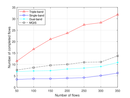
Figure 2: Number of completed flows versus different numbers of requested flows.

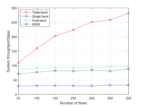
Figure 3: System throughput versus different numbers of requested flows.

From Fig. 2, we can see that the trend of the proposed triple-band scheme curve is rising with the increased number of flows. The more flows that need to be scheduled, the more flows can be scheduled simultaneously and the more spatial reuse comes into play. Because of the system capacity limitation, the growth of the number of completed flows of the triple-band scheduling scheme gets slowed down with the further increasing of the number of offered flows. Compared with our proposed scheme, although there is also a trend of growth in the number of completed flows of MQIS, the increase is much slower than that of the proposed scheme. The ability of MQIS to schedule flows is inferior to the proposed triple-band scheme, because MQIS cannot schedule flows without interruption, which wastes a certain amount of the time resource. For the dual-band scheme and the single-band scheme, there are also slower growths in the number of completed flows along the x-axis direction. This is because the single-band scheme does not exploit the THz band, and its ability to schedule the flows is thus limited. Besides, the completed flows of the dual-band scheme and the single-band scheme are both relatively few. Some flows with large QoS requirements cannot be scheduled without the THz band. When the number of flows is 350, the proposed triple-band scheduling scheme improves the number of completed flows by 56.3% compared with the MQIS scheme, by 64.1% compared with the dual-band scheme, and by 79.7% compared with the single-band scheme.

From Fig. 3, we can observe that the trend of the throughput curves is similar to the trend of the number of completed flows. There is a certain gap between the completed-flow numbers of the four schemes. and the gaps of throughput curves are similar as that in Fig. 2 except for the dual-band scheme. For the dual-band scheme, we set a very large bandwidth for one of its frequency bands (even larger than $W^{me}$), so its performance on the system throughput can be better than MQIS. Specifically, when the number of flows is 350, the proposed triple-band scheduling scheme improves the system throughput by 67.9% compared with the dual-band scheme, by 64.3% compared with MQIS, and by 87.5% compared with the single-band scheme.

In Fig. 4 and Fig. 5, the number of flows is fixed at 350. The number of time slots is increased from 500 to 4500. With the number of TSs is increased, Fig. 4 and Fig. 5 plot simulation results of the number of completed flows and system throughput.

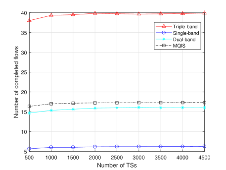
Figure 4: Number of completed flows versus different numbers of time slots.

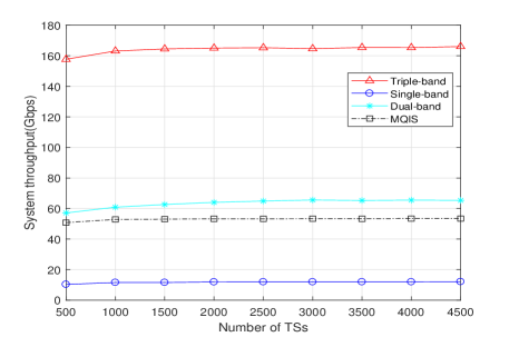
Figure 5: System throughput versus different numbers of time slots.

From Fig. 4 and Fig. 5, we can see that the number of completed flows and system throughput have the same trend with increased number of TSs. These schemes also exhibit similar trends. When the number of time slots starts to increase, both the number of completed flows and system throughput increase. When the number of time slots is increased over a certain value ( i.e., to 2000 in Fig. 4 and Fig. 5), the number of completed flows and system throughput become saturated and do not increase significantly anymore. This shows that properly extending the duration of each frame is conducive to improving the transmission performances, but the improvement is limited. In this case, the numbers of completed flows of the proposed triple-band scheduling scheme, MQIS, the dual-band scheme and the single-band scheme can be up to 40, 18, 16 and 7, respectively. Furthermore, it is not necessary to set a very large value for the number of TSs.

In Fig. 6 and Fig. 7, the number of flows is set to 350 and the number of time slots is set to 2000. We evaluate the impact of the reference distance of THz communications, i.e., $D_{ref}^{THz}$, which is set to 30m, 40m, and 50m. With increased number of flows, Fig. 6 and Fig. 7 plot the number of completed flows and system throughput under different $D_{ref}^{THz}$ values.

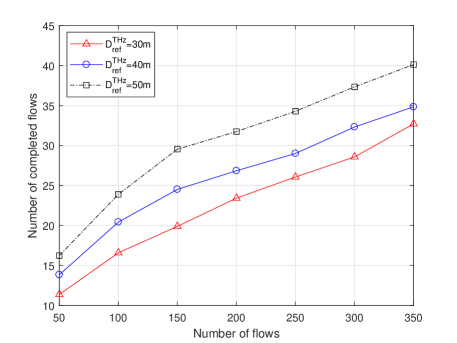
Figure 6: Number of completed flows versus different reference distances of THz communications.

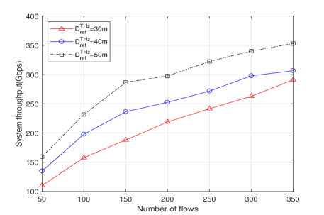
Figure 7: System throughput versus different reference distances of THz communications.

From Fig. 6 and Fig. 7, we can see that the number of completed flows and system throughput exhibit similar results as $D_{ref}^{THz}$ is increased. The larger the $D_{ref}^{THz}$, the more flows can be scheduled simultaneously and the larger the system throughput. If the reference distance $D_{ref}^{THz}$ is large, there will be more flows that can be scheduled in the THz band, leading to more completed flows and larger throughput. We can also observe that the gap between the curves of $D_{ref}^{THz}=40$m and $D_{ref}^{THz}=30$m is bigger than the gap between the curves of $D_{ref}^{THz}=50$m and $D_{ref}^{THz}=40$m. The performance improvement decreases with further increased $D_{ref}^{THz}$, which shows that the performance improvement caused by $D_{ref}^{THz}$ is also limited. However, we need to consider the actual transmission characteristics of the THz band, while $D_{ref}^{THz}$ cannot be too large. If the distance of the THz communications is too large, the higher propagation loss will cause more flow transmission to fail.

In Fig. 8 and Fig. 9, the number of flows is set to 350 and the number of time slots is set to 2000. Abscissas of these two figures are $-\lg(\sigma^{THz})$, which is varied from 0 to 6. $-\lg(\sigma^{mm})$ and $-\lg(\sigma^{me})$ are about two orders of magnitude lower than $-\lg(\sigma^{THz})$, so they are varied from 2 to 8 with $-\lg(\sigma^{THz})$ is varied from 0 to 6. With decreased threshold, Fig. 8 and Fig. 9 plot the number of completed flows and system throughput achieved by the four schemes.

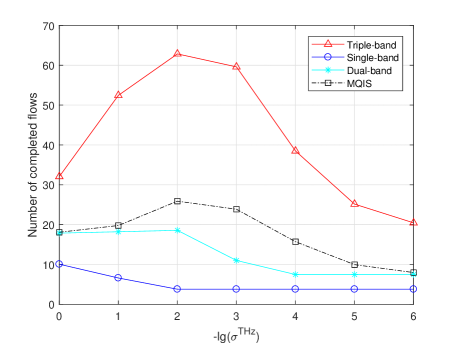
Figure 8: Number of completed flows versus different thresholds.

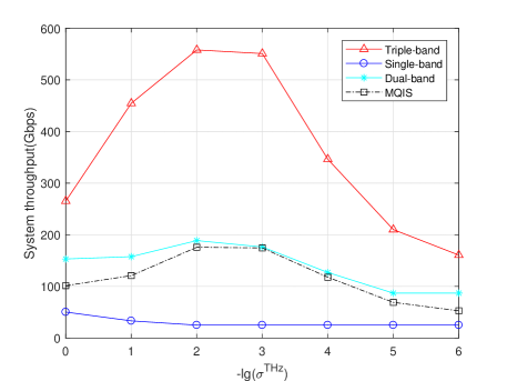
Figure 9: System throughput versus different thresholds.

From Fig. 8 and Fig. 9, we can see that trends of the number of completed flows and system throughput are similar with the decrease of interference threshold. For the triple-band scheme, when thresholds start to decrease, both the number of completed flows and system throughput increase. Properly decreasings of thresholds can avoid simultaneous scheduling of some flows that have serious interference between themselves. And then their transmission rates can be increased, which will lead to more flows to be completed more quickly. When $\sigma^{THz}$, $\sigma^{me}$ and $\sigma^{mm}$ are decreased to a certain order of magnitude ( i.e., $\sigma^{THz}=10^{-2}$, $\sigma^{me}=\sigma^{mm}=10^{-4}$ in Fig. 4 and Fig. 5), the number of completed flows and system throughput start to decrease significantly. A too small threshold will weaken the advantages of spatial reuse and reduce flows that can be scheduled simultaneously. Therefore, the appropriate actual interference threshold is important for the transmission performance. In the case of our simulation study, actual interference thresholds $\sigma^{THz}$ of $10^{-2}$ order, $\sigma^{me}$ and $\sigma^{mm}$ of $10^{-4}$ order seem to be suitable. For the single-band scheme, their scheduling capabilities have been limited by their specific designs when the number of flows is 350. Hence, the number of completed flows and system throughput of this scheme decrease with decreased threshold.

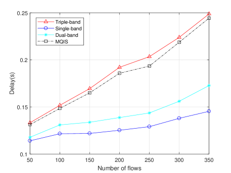
Figure 10: Delay versus different numbers of requested flows.

In Fig. 10, the number of time slots is set to 2000. The abscissas of the figure is the number of requested flows, which is varied from 50 to 350. As the number of requested flows is increased, Fig. 10 plots the simulation results of the delay of different schemes.

From Fig. 10, we can see that the trends of all the schemes curve are rising with the increased number of flows. Compared with our proposed scheme, other schemes have different advantages in terms of delay. However, combined with the advantage of the proposed triple-band scheme shown in Fig. 2, the advantages of other schemes in terms of delay are of little significance. It is obvious that the more scheduled flows, the greater the delay of the scheme. When the number of flows is 350, the delay of the proposed triple-band scheduling scheme is 0.25s, and it is the delay size that allows communications between BSs.

VII Conclusions

In this paper, we considered the problem of scheduling a large number of flows with diverse QoS requirements over three frequency bands (i.e., the 28GHz band, E-band, and THz band). To maximize the number of flows while satisfying their QoS requirements, we proposed the triple-band scheduling scheme, which can schedule flows to be concurrently transmitted and reduce the waste of resource, while considering the QoS requirements and transmission ranges of the flows. Extensive simulations showed that our proposed scheme outperformed three baseline schemes on the number of completed flows and system throughput. However, the complexity of THz transmission itself and the high cost of transmission equipment limit the communication, and we require further research and follow-up. In the future work, we will consider a more realistic scene and transmission model. Besides, we will do the performance verification of our algorithm on the actual system platform to further demonstrate the practicality of our scheme.

References

- [1] R. Ansari, H. Pervaiz, C. Chrysostomou, S. Hassan, A. Mahmood, and M. Gidlund, “Control-Data separation architecture for dual-band mmWave networks: A new dimension to spectrum management,” IEEE Access, vol. 7, pp. 34925–34937, 2019.
- [2] R. Baldemair, T. Irnich, K. Balachandran, E. Dahlman, G. Mildh, Y. Seln, S. Parkvall, M. Meyer, and A. Osseiran, “Ultra-dense networks in millimeter-wave frequencies,” IEEE Commun. Mag., vol. 53, no. 1, pp. 202–208, Jan. 2015.
- [3] H. Zhou, S. Mao, and P. Agrawal, “Approximation algorithms for cell association and scheduling in femtocell networks,” IEEE Trans. Emerging Topics Comput., vol.3, no.3, pp.432–443, Sept. 2015.
- [4] Z. Yan, W. Zhou, S. Chen, and H. Liu, “Modeling and analysis of two-tier HetNets with cognitive small cells,” IEEE Access, vol. 5, pp. 2904–2912, 2017.
- [5] M. R. Akdeniz, Y. Liu, M. K. Samimi, S. Sun, S. Rangan, T. S. Rappaport and E. Erkip, “Millimeter wave channel modeling and cellular capacity evaluation,” IEEE J. Sel. Areas Commun., vol. 32, no. 6, pp. 1164–1179, June 2014.
- [6] Z. Xiao, T. He, P. Xia, and X. -G. Xia, “Hierarchical codebook design for beamforming training in millimeter-wave communication,” IEEE Trans. Wireless Commun., vol. 15, no. 5, pp. 3380–3392, May 2016.
- [7] I. F. Akyildiz, J. M. Jornet, and C. Han, “Teranets: Ultra-broadband communication networks in the Terahertz band,” IEEE Trans. Wireless Commun., vol. 21, no. 4, pp. 130–135, Aug. 2014.
- [8] S. Singh, R. Mudumbai, and U. Madhow, “Distributed coordination with deaf neighbors: Efficient medium access for 60 GHz mesh networks,” in Proc. IEEE INFOCOM’10, San Diego, CA, Mar. 2010, pp. 1–9.
- [9] C. Sum, Z. Lan, R. Funada, J. Wang, T. Baykas, M. A. Rahman, and H. Harada, “Virtual time-slot allocation scheme for throughput enhancement in a millimeter-wave multi-Gbps WPAN system,” IEEE J. Sel. Areas Commun., vol. 27, no. 8, pp. 1379–1389, Oct. 2009.
- [10] Z. He and S. Mao “Adaptive multiple description coding and transmission of uncompressed video over 60GHz networks,” ACM Mobile Computing and Communications Review (MC2R), vol.18, no.1, pp.14–24, Jan. 2014.
- [11] R. Taori, and A. Sridharan, “Point-to-multipoint in-band mmwave backhaul for 5G networks,” IEEE Commun. Mag., vol. 53, no. 1, pp. 195–201, Jan. 2015.
- [12] E. Arribas, A. Anta, D. Kowalski, V. Mancuso, and et al., “Optimizing mmWave wireless backhaul scheduling,” IEEE Transactions on Mobile Computing, vol. 19, no. 10, pp. 2409–2428, Oct. 2020.
- [13] D. Yuan, H. Lin, J. Widmer, and M. Hollick, “Optimal and approximation algorithms for joint routing and scheduling in millimeter-Wave cellular networks,” IEEE/ACM Transactions on Networking , vol. 28, no. 5, pp. 2188–2202, Oct. 2020.
- [14] C. Fang, C. Madapatha, B. Makki, and T. Svensson, “Joint scheduling and throughput maximization in self-backhauled millimeter wave cellular networks” in Proc. IEEE ISWCS’17, Berlin, Germany, Sept. 2021, pp. 1–3.
- [15] Q. Hu, and D. M. Blough, “On the feasibility of high throughput mmWave backhaul networks in urban areas” IEEE Trans. Wireless Commun., in Proc. IEEE ICNC’10, Big Island, HI, USA, Feb. 2020, pp. 1–3.
- [16] Y. Niu, W. Ding, H. Wu, Y. Li, X. Chen, B. Ai, and Z. Zhong, “Relay-assisted and QoS aware scheduling to overcome blockage in mmWave backhaul networks,” IEEE Trans. Veh. Technol., vol. 68, no. 2, pp. 1733–1744, Feb. 2019.
- [17] K. Ntontin, and C. Verikoukis, “Toward the performance enhancement of microwave cellular networks through THz links,” IEEE Trans. Veh. Technol., vol. 66, no. 7, pp. 5635–5646, July 2017.
- [18] H. Jiang, Y. Niu, B. Ai, Z. Zhong, and S. Mao, “QoS-Aware bandwidth allocation and concurrent scheduling for terahertz wireless backhaul networks,” IEEE Access, vol. 8, pp. 125814–125825, July 2020.
- [19] Z. Zhang, H. Zhang, K. Long, and G. K. Karagiannidis, “Improved Whale Optimization Algorithm based Resource Scheduling in NOMA THz Networks,” in Proc. IEEE GLOBECOM’64, Madrid, Spain, Dec. 2021, pp. 1–6.
- [20] P. Zhou, X. Fang, X,Wang, and Li Yan, “Multi-beam transmission and dual-band cooperation for control/data plane decoupled WLANs,” IEEE Trans. Veh. Technol., vol. 68, no. 10, pp. 9806–9819, Oct. 2019.
- [21] S. Y. Geng, J. Kivinen, X. W. Zhao, and P. Vainikainen, “Millimeter wave propagation channel characterization for short-range wireless communications,” IEEE Trans. Veh. Technol., vol. 58, no. 1, pp. 3–13, Jan. 2009.
- [22] J. Qiao, X. S. Shen, J. W. Mark, Q. Shen, Y. He, and L. Lei, “Enabling device-to-device communications in millimeter-wave 5G cellular networks,” IEEE Commun. Mag., vol. 53, no. 1, pp. 209–215, Jan. 2015.
- [23] J. Qiao, L. X Cai, X. Shen, and J. Mark, “STDMA-based scheduling algorithm for concurrent transmissions in directional millimeter wave networks,” in Proc. IEEE ICC’12, Ottawa, Canada, June 2012, pp. 5221–5225.
- [24] Y. Niu, Y. Liu, Y. Li, X. Chen, Z. Zhong and Z. Han, “Device-to-Device communications enabled energy efficient multicast scheduling in mmWave small cells,” IEEE Trans. Commun., vol. 66, no. 3, pp. 1093–1109, Mar. 2018.
- [25] Y. Zhu, Y. Niu, J. Li, D. O. Wu, Y. Li, and D. Jin, “QoS-aware scheduling for small cell millimeter wave mesh backhaul,” in Proc. IEEE ICC’16, Kuala Lumpur, Malaysia, May 2016, pp. 1–6.
- [26] Y. Niu, C. Gao, Y. Li, L. Su, D. Jin, and A. V. Vasilakos, “Exploiting device-to-Device communications in joint scheduling of access and backhaul for mmWave small cells,” IEEE J. Sel. Areas Commun., vol. 33, no. 10, pp. 2052–2069, Oct. 2015.
- [27] Y. Wang, Atmospheric propagation characteristics and capacity analysis of terahertz wave. Doctor, Chinese academy of engineering physics, Beijing China, 2017.
- [28] R. Piesiewicz, T. Kleine Ostmann, and T. Kurner, “Short range ultra broadband terahertz communications: Concepts and perspectives,” IEEE Antennas Propag. Mag., vol. 49, no. 6, pp. 24–39, Dec. 2007.
- [29] J. M. Jornet, and I. F. Akyildiz, “Channel modeling and capacity analysis for electromagnetic wireless nanonetworks in the terahertz band,” IEEE Trans. Wireless Commun., vol. 10, no. 10, pp. 3211–3221, Oct. 2011.
- [30] J. Wang, Z. Lan, C. Pyo, T. Baykas, C. Sum, M. Rahman, J. Gao, R. Funada, F. Kojima, and S. Kato, “Beam codebook based beamforming protocol for multi-Gbps millimeter-wave WPAN systems,” IEEE J. Sel. Areas Commun., vol. 27, no. 8, pp. 1390–1399, Oct. 2009.
- [31] M. D. Renzo, “Stochastic geometry modeling and analysis of multitier millimeter wave cellular networks,” IEEE Trans. Wireless Commun., vol. 14, no. 9, pp. 5038–5057, Sept. 2015.
- [32] B. K. Jung, N. Dreyer, and et al., “Simulation and automatic planning of 300 GHz backhaul links,” in Proc. 44th Int. Conf. Infr., Millim., THz. Waves (IRMMW-THz), Paris, France, 2019, pp. 1-3, doi: 10.1109/IRMMW-THz.2019.8873734.
- [33] W. Ding, Y. Niu, H. Wu, Y. Li, and Z. Zhong, “QoS-Aware full-Duplex concurrent scheduling for millimeter wave wireless backhaul networks,” IEEE Access, vol. 6, pp. 25313–25322, Apr. 2018.