So3krates: Equivariant attention for interactions on arbitrary length-scales in molecular systems

Abstract

The application of machine learning methods in quantum chemistry has enabled the study of numerous chemical phenomena, which are computationally intractable with traditional ab-initio methods. However, some quantum mechanical properties of molecules and materials depend on non-local electronic effects, which are often neglected due to the difficulty of modeling them efficiently. This work proposes a modified attention mechanism adapted to the underlying physics, which allows to recover the relevant non-local effects. Namely, we introduce spherical harmonic coordinates (SPHCs) to reflect higher-order geometric information for each atom in a molecule, enabling a non-local formulation of attention in the SPHC space. Our proposed model So3krates – a self-attention based message passing neural network – uncouples geometric information from atomic features, making them independently amenable to attention mechanisms. Thereby we construct spherical filters, which extend the concept of continuous filters in Euclidean space to SPHC space and serve as foundation for a spherical self-attention mechanism. We show that in contrast to other published methods, So3krates is able to describe non-local quantum mechanical effects over arbitrary length scales. Further, we find evidence that the inclusion of higher-order geometric correlations increases data efficiency and improves generalization. So3krates matches or exceeds state-of-the-art performance on popular benchmarks, notably, requiring a significantly lower number of parameters (0.25–0.4x) while at the same time giving a substantial speedup (6–14x for training and 2–11x for inference) compared to other models.

1 Introduction

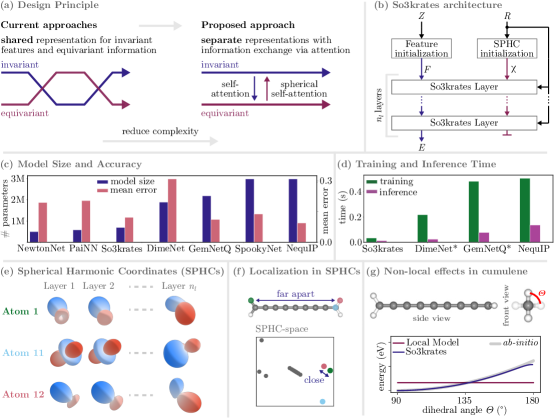
Figure 1: (a) Design principle of our proposed message-passing scheme, where invariant features $\mathbf{f}$ and equivariant information - represented by spherical harmonic coordinates (SPHCs) $\bm{\chi}$ - are separate and exchange information via (spherical) self-attention. (b) Overview of the So3krates architecture. (c) Comparison of prediction accuracy and model size of different architectures. (d) Comparison of training and inference times of different architectures. (e) Illustration of learned SPHCs at different layers of the So3krates architecture. (f) Low-dimensional projection of atomic SPHCs, showing that atoms far apart in Euclidean space can be mapped close together in SPHC space. (g) In contrast to local models, So3krates is able to learn the long-range correlations between hydrogen rotors in cumulene and reproduces the ab-initio ground truth faithfully.

Atomistic simulations use long time-scale molecular dynamics (MD) trajectories to predict macroscopic properties that arise from interactions on the microscopic scale [1, 2, 3]. Their predictive reliability is determined by the accuracy of the underlying force field (FF), which needs to be queried at every time step. This quickly becomes a computational bottleneck if the forces are determined from first principles, which may be required for accurate results. To that end, machine learning FFs (MLFFs) offer a computationally more efficient, yet accurate empirical alternative to expensive ab-initio methods [4, 5, 6, 7, 8, 9, 10, 11, 12, 13, 14, 15, 16, 17, 18, 19, 20, 21, 22, 23, 2, 24].

In recent years, Geometric Deep Learning has become a popular design paradigm, which exploits relevant symmetry groups of the underlying learning problem by incorporating a geometric prior [12, 25, 26]. This effectively restricts the learnable functions of the model to a subspace with a meaningful inductive bias. Prominent examples for such models are e.g. convolutional neural networks (CNNs) [27], which are equivariant w. r. t. the group of translations, or graph neural networks (GNNs) [28], which are invariant w. r. t. node permutation.

For molecular property prediction, it has been shown that equivariance w. r. t. the 3D rotation group $\mathrm{SO}(3)$ greatly improves data efficiency and accuracy of the learned FFs [29, 30, 31, 32]. To achieve equivariance, architectures either rely on feature expansions in terms of spherical harmonics (SH) [33] or explicitly include (dihedral) angles [29, 34]. While the latter scales quadratically (cubically) in the number of neighboring atoms and has been shown to be geometrically incomplete [35], the calculation of spherical harmonics scales only linear in the number of neighboring atoms, which makes them a fast and accurate alternative [32, 30, 36].

However, current higher-order geometric representations based on SHs usually result in expensive transformations, since an individual feature channel per SH degree (and order) is required. As a result, going to higher degrees is computationally expensive and comes at the price of increasing complexity, resulting in state-of-the-art (SOTA) models with millions of parameters [32, 30, 34]. However, in order to be applicable to large molecular structures, models are required to be both efficient and accurate on all length scales.

Non-local electronic effects have been outlined as one of the major challenges for a new generation of MLFFs [21]. They result in non-local, higher-order geometric relations between atoms. Most current architectures implicitly assume locality of interactions (expressed through a local neighborhood), which prohibits an efficient description of all relevant atomic interactions at larger scales. Simply increasing the cutoff radius used to determine local neighborhoods is not an adequate solution, since it only shifts the problem to larger length scales [30].

In this work, we propose spherical harmonic coordinates (SPHCs), which encode higher-order geometric information for each node in a molecular graph (Fig. 1e). This is in stark contrast to current approaches, which consider molecules as three-dimensional point clouds with learned features and fixed atomic coordinates: we propose to make the SPHCs themselves a learned quantity. Through localization in the space of SPHCs (Fig. 1f), models are able to efficiently describe electronic effects that are non-local in three-dimensional Euclidean space (Fig. 1g).

We then present So3krates (Fig. 1b), a self-attention based message-passing neural network (MPNN), which decouples atomic features and SPHCs and updates them individually (Fig. 1a). This resembles ideas from equivariant graph neural networks [25], but allows to go to arbitrarily high geometric orders. The separation of higher-order geometric and feature information allows to overcome the parametric and computational complexity usually encountered in models with higher-order geometric representations, since we only require a single feature channel (instead of one per SH degree and order). Thus, So3krates resembles some early architectures like SchNet [10] or PhysNet [19] in parametric simplicity. We further show that So3krates outperforms the popular sGDML [38] kernel model by a large margin in the low-data regime, a domain which has so far been considered to be dominated by kernel machines [21]. Numerical evidence suggests that the data efficiency of So3krates is directly related to the maximal degree of geometric information encoded in the SPHCs. We then apply So3krates to the well-established MD17 benchmark and show that our model achieves SOTA results, despite is light-weight structure and having only 0.25–0.4x the number of parameters of competitive architectures (Fig. 1c), while achieving speedups of 6–14x and 2–11x for training and inference, respectively (Fig. 1d).

Although we focus on quantum chemistry applications in this work, the developed methods are also applicable to other fields where long-ranged correlations in three-dimensional data are relevant. For example, models based on SPHCs may also be applicable to tasks like 3D shape classification or computer vision.

2 Preliminaries and Related Work

In the following, we review the most important concepts our method is based upon and relate it to prior work.

Message Passing Neural Networks

MPNNs [14] carry over many of the benefits of convolutions to unstructured domains and have thus become one of the most promising approaches for the description of molecular properties. Their general working principle relies on the repeated iteration of message passing (MP) steps, which can be phrased as follows [25, 14]

$$\mathbf{m}_{ij} =m(\mathbf{f}_{i},\mathbf{f}_{j},\bm{r}_{ij})$$ (1)

$$\mathbf{m}_{i} =\sum_{j\in\mathcal{N}(i)}\mathbf{m}_{ij}$$ (2)

$$\mathbf{f}_{i}^{\prime} =u(\mathbf{f}_{i},\mathbf{m}_{i})\,.$$ (3)

Here, $\mathbf{m}_{ij}$ is the message between atoms $i$ and $j$ computed with the message function $m(\cdot)$, $\mathbf{m}_{i}$ is the aggregation of all messages in the neighborhood $\mathcal{N}(i)$ of atom $i$, and $u(\cdot)$ is an update function returning updated features $\mathbf{f}_{i}^{\prime}$ based on the current features $\mathbf{f}_{i}$ and message $\mathbf{m}_{i}$. The neighborhood $\mathcal{N}(i)$ consists of all atoms which lie within a given cutoff radius around the atomic position $\bm{r}_{i}$, which ensures linear scaling in the number of atoms $n$. While earlier variants parametrized messages only in terms of inter-atomic distances [13, 19], more recent approaches also take higher-order geometric information into account [39, 29, 25, 31, 32, 40].

Molecules as Point Clouds

A molecule can be considered as a point cloud of $n$ atoms $\mathcal{P}_{3D}(\mathcal{R},\mathcal{F})$, where $\mathcal{R}=(\bm{r}_{1},...\bm{r}_{n})$ denotes the set of atomic positions $\bm{r}_{i}\in\mathbb{R}^{3}$ and $\mathcal{F}=(\mathbf{f}_{1},\dots,\mathbf{f}_{n})$ is the set of rotationally invariant atomic descriptors, or features, $\mathbf{f}_{i}\in\mathbb{R}^{F}$. We write the distance vector pointing from the position of atom $i$ to the position of atom $j$ as $\bm{r}_{ij}=\bm{r}_{j}-\bm{r}_{i}$, the distance as $r_{ij}=\lVert\bm{r}_{ij}\rVert_{2}$ and the normalized distance vector as $\hat{\bm{r}}_{ij}=\bm{r}_{ij}/r_{ij}$. Given the point cloud, a density over Euclidean space assigning a vector value to each point $\bm{r}$ can be constructed as

$$\bm{\rho}(\bm{r})=\sum_{i=1}^{n}\delta(\lVert\bm{r}_{i}-\bm{r}\rVert_{2})\cdot\mathbf{f}_{i}\,,$$ (4)

where $\delta$ is the Dirac delta function. It can be shown that applying a convolutional filter on $\bm{\rho}(\bm{r})$ resembles the update steps used in MPNNs [41].

Equivariance

Given a set of transformations that act on a vector space $\mathbb{A}$ as $S_{g}:\mathbb{A}\mapsto\mathbb{A}$ to which we associate an abstract group $G$, a function $f:\mathbb{A}\mapsto\mathbb{B}$ is said to be equivariant w. r. t. $G$ if

$$f(S_{g}x)=T_{g}f(x)\,,$$ (5)

where $T_{g}:\mathbb{B}\mapsto\mathbb{B}$ is an equivalent transformation on the output space [25]. Thus, in order to say that $f$ is equivariant, it must hold that under transformation of the input, the output transforms “in the same way”. While equivariance has been a popular concept in signal processing for decades (cf. e.g. [42] or wavelet neural networks [43]), recent years have seen efforts to design group equivariant NNs and kernel methods, since respecting relevant symmetries builds an important inductive bias [44, 45, 12]. Examples are CNNs [27] which are equivariant w. r. t. translation, GNNs [28, 14] which are invariant ($T_{g}=\mathbb{I}$) w. r. t. permutation, or architectures which are equivariant w. r. t. the $\mathrm{SO}(3)$ group [33, 46, 36, 31, 25]. In this work, we consider the $\mathrm{SO}(3)$ group of rotations, such that $\mathbb{A}$ is the Euclidean space $\mathbb{R}^{3}$, where the corresponding group actions are given by rotation matrices $R_{\theta}\in\mathbb{R}^{3\times 3}$.

Spherical Harmonics

The spherical harmonics are special functions defined on the surface of the sphere $S^{2}=\{\hat{\bm{r}}\in\mathbb{R}^{3}:\lVert\hat{\bm{r}}\rVert_{2}=1\}$ and form an orthonormal basis for the irreducible representations (irreps) of $\mathrm{SO}(3)$. In the context of tensor field networks [33], they have been introduced as elementary building blocks for $\mathrm{SO}(3)$-equivariant neural networks. The spherical harmonics are commonly denoted as $Y_{l}^{m}(\hat{\bm{r}}):S^{2}\mapsto\mathbb{R}$, where the degree $l$ determines all possible values of the order $m\in\{-l,\dots,+l\}$. They transform under rotation as

$$Y_{l}^{m}(R_{\theta}\,\hat{\bm{r}})=\sum_{m^{\prime}}D_{mm^{\prime}}^{l}(R_{\theta})\,Y_{l}^{m^{\prime}}(\hat{\bm{r}})\,,$$ (6)

where $D_{mm^{\prime}}^{l}(R_{\theta})$ are the entries of the Wigner-D matrix $\mathbf{D}^{l}(R_{\theta})\in\mathbb{R}^{(2l+1)\times(2l+1)}$ [47]. Based on the spherical harmonics, we define a vector-valued function $\bm{Y}^{(l)}:S^{2}\mapsto\mathbb{R}^{2l+1}$ for each degree $l$, with entries $Y_{l}^{m}$ for all valid orders $m$ of a given degree $l$. Since $\bm{Y}^{(l)}(R_{\theta}\,\hat{\bm{r}})=\mathbf{D}^{l}(R_{\theta})\bm{Y}^{(l)}(\hat{\bm{r}})$ (cf. eq. (6)), $\bm{Y}^{(l)}$ is equivariant w. r. t. $\mathrm{SO}(3)$.

Tensor Product Contractions

The irreps $\bm{Y}^{(l_{1})}$ and $\bm{Y}^{(l_{2})}$ can be coupled by computing their tensor product $\bm{Y}^{(l_{1})}\otimes\bm{Y}^{(l_{2})}$, which can equivalently be expressed as a direct sum [33, 48]

$$\bm{Y}^{(l_{1})}\otimes\bm{Y}^{(l_{2})}=\bigoplus_{l_{3}=\lvert l_{1}-l_{2}\rvert}^{l_{1}+l_{2}}\overbrace{\bm{\tilde{Y}}^{(l_{3})}}^{\coloneqq\left(\bm{Y}^{(l_{1})}\otimes_{l_{3}}\bm{Y}^{(l_{2})}\right)}\,,$$ (7)

where the entry of order $m_{3}$ for the coupled irreps $\bm{\tilde{Y}}^{(l_{3})}$ is given by

$$\tilde{Y}_{m_{3}}^{l_{3}}=\sum_{m_{1}=-l_{1}}^{l_{1}}\sum_{m_{2}=-l_{2}}^{l_{2}}C_{m_{1},m_{2},m_{3}}^{l_{1},l_{2},l_{3}}Y_{m_{1}}^{l_{1}}Y_{m_{2}}^{l_{2}}\,,$$ (8)

and $C_{m_{1},m_{2},m_{3}}^{l_{1},l_{2},l_{3}}$ are the so-called Clebsch-Gordon coefficients. In the following, we will denote the tensor product of degrees $l_{1}$ and $l_{2}$ followed by “contraction” to $l_{3}$ (meaning the irreps of degree $l_{3}$ in the direct sum representation of their tensor product) as $\left(\bm{Y}^{(l_{1})}\otimes_{l_{3}}\bm{Y}^{(l_{2})}\right)$, which is a mapping of the form $\mathbb{R}^{(2l_{1}+1)\times(2l_{2}+1)}\mapsto\mathbb{R}^{2l_{3}+1}$, since $m_{3}\in\{-l_{3},\dots l_{3}\}$.

3 Methods

In the following, we describe the main methodological contributions of this work. We introduce the concept of an adapted point cloud $\mathcal{P}_{3D}(\mathcal{R},\mathcal{X},\mathcal{F})$, which incorporates the set of spherical harmonics coordinates (SPHCs) $\mathcal{X}=(\bm{\chi}_{1},\dots,\bm{\chi}_{n})$ (see below) in addition to features $\mathcal{F}$ and Euclidean coordinates $\mathcal{R}$. However, contrary to $\mathcal{R}$, SPHCs $\mathcal{X}$ are refined during the message passing updates. Having SPHCs as part of the molecular point cloud extends the idea of current MPNNs, which learn message functions on $\mathcal{R}$, only. Instead, we learn a message function $m$ (cf. eq. (1)) on both, the (fixed) atomic coordinates $\mathcal{R}$ as well as on the SPHCs $\mathcal{X}$. This adapted message-passing scheme allows to learn non-local geometric corrections. Based on these design principles, we propose the So3krates architecture.

Initialization

Feature vectors are initialized from the atomic numbers $z_{i}\in\mathbb{N}$ (denoting which chemical element an atom belongs to) by an embedding map

$$\mathbf{f}_{i}=f_{\mathrm{emb}}(z_{i}),$$ (9)

where $f_{\mathrm{emb}}:\mathbb{N}\mapsto\mathbb{R}^{F}$. We define SPHCs $\bm{\chi}$ as the concatenation of degrees $\mathcal{L}\coloneqq\{l_{\mathrm{min}},\dots,l_{\mathrm{max}}\}$

$$\bm{\chi}=[\underbrace{\bm{\chi}{{}^{(l_{\mathrm{min}})}}}_{\in\mathbb{R}^{2l_{\mathrm{min}}+1}},\dots,\underbrace{\bm{\chi}{{}^{(l_{\mathrm{max}}})}}_{\in\mathbb{R}^{2l_{\mathrm{max}}+1}}]\in\mathbb{R}^{(l_{\mathrm{max}}-l_{\mathrm{min}}+1)^{2}},$$ (10)

such that their transformation under rotation can be expressed in terms of concatenated Wigner-D matrices (see appendix A.1). The short-hand $\bm{\chi}^{(l)}\in\mathbb{R}^{2l+1}$ refers to the subset of SPHCs with degree $l$. They are initialized as

$$\bm{\chi}_{i}^{(l)}=\frac{1}{\mathcal{C}_{i}}\sum_{j\in\mathcal{N}(i)}\phi_{r_{\mathrm{cut}}}(r_{ij})\cdot\bm{Y}^{(l)}(\hat{\bm{r}}_{ij}),$$ (11)

where $\mathcal{C}_{i}=\sum_{j\in\mathcal{N}(i)}\phi_{r_{\mathrm{cut}}}(r_{ij})$, $\phi_{r_{\mathrm{cut}}}:\mathbb{R}\mapsto\mathbb{R}$ is the cosine cutoff function [6], and the sum runs over the neighborhood $\mathcal{N}(i)$ of atom $i$.

Message Passing Update

Two branches of attention-weighted MP steps are defined for the feature vectors $\mathbf{f}$ and SPHCs $\bm{\chi}$ (see Fig. 1a). After initialization (eqs. (9) and (11)), the features are updated as

$$\mathbf{f}_{i}^{\prime}=\mathbf{f}_{i}+\sum_{j\in\mathcal{N}(i)}\phi_{r_{\mathrm{cut}}}(r_{ij})\cdot\alpha_{ij}\cdot\mathbf{f}_{j}\,,$$ (12)

where $\alpha_{ij}\in\mathbb{R}$ are self-attention [49, 50] coefficients (see below). In analogy to the feature vectors, it is possible to define an MP update for the SPHCs as

$$\bm{\chi}_{i}^{\prime\,(l)}=\bm{\chi}_{i}^{(l)}+\sum_{j\in\mathcal{N}(i)}\phi_{r_{\mathrm{cut}}}(r_{ij})\cdot\alpha^{(l)}_{ij}\cdot\bm{Y}^{(l)}(\hat{\bm{r}}_{ij})\,,$$ (13)

where individual attention coefficients $\alpha_{ij}^{(l)}\in\mathbb{R}$ for each degree of the SPHCs are computed using multi-head attention [49]. However, with this definition, both MP updates are limited to local neighborhoods $\mathcal{N}(i)$. To be able to model non-local effects, we introduce the SPHC distance matrix $\mathbf{X}\in\mathbb{R}^{n\times n}$ with entries $\chi_{ij}=\lVert\bm{\chi}_{i}-\bm{\chi}_{j}\rVert_{2}$, i.e. distances between two atoms $i$ and $j$ in SPHC space for all possible pair-wise combinations of $n$ atoms. To have uniform scales, we further apply the $\mathrm{softmax}$ along each row of $\mathbf{X}$ to generate a rescaled matrix $\tilde{\mathbf{X}}=\mathrm{softmax}(\mathbf{X})$ with entries $\tilde{\chi}_{ij}$. A polynomial cutoff function $\phi_{\tilde{\chi}_{\rm cut}}$ [29] is then applied to $\tilde{\mathbf{X}}$ to define spherical neighborhoods $\mathcal{N}_{\bm{\chi}}(i)$ (see A.2), which may include atoms that are far away in Euclidean space (see Fig. 1f). The spherical cutoff distance is chosen as $\tilde{\chi}_{\rm cut}=1/n$ to ensure that spherical neighborhoods remain small, even when going to larger molecules. We then incorporate non-local geometric corrections into the MP update of the SPHCs as

$${\bm{\chi}}_{i}^{\prime\,(l)}=\bm{\chi}_{i}^{(l)}+\underbrace{\sum_{j\in\mathcal{N}(i)}\phi_{r_{\mathrm{cut}}}(r_{ij})\cdot\alpha_{ij}^{(l)}\cdot\bm{Y}^{(l)}(\hat{\bm{r}}_{ij})}_{\text{local in $\mathbb{R}^{3}$}}+\underbrace{\sum_{j\in\mathcal{N}_{\bm{\chi}}(i)}\phi_{\tilde{\chi}_{\rm cut}}(\tilde{\chi}_{ij})\cdot\alpha_{ij}^{(l)}\cdot\bm{Y}^{(l)}(\hat{\bm{r}}_{ij})}_{\text{local in ${\bm{\chi}}$, but non-local in $\mathbb{R}^{3}$}}\,.$$ (14)

We will show in the first part of the experiments, how geometric corrections from SPHC space allow for modelling non-local quantum effects, inaccessible to current architectures. In the second part, we use a So3krates model without geometric corrections, which makes it a traditional MPNN in the sense of only localizing in $\mathbb{R}^{3}$. We find this architecture to be highly parameter, data and time efficient while capable of reaching SOTA results.

Spherical Filter and Self-Attention

The self-attention coefficients in eqs. (12)–(14) are calculated as

$$\alpha_{ij}=\mathbf{f}_{i}^{T}(\mathbf{w}_{ij}\odot\mathbf{f}_{j})/{\sqrt{F}}\,,$$ (15)

where $\mathbf{w}_{ij}\in\mathbb{R}^{F}$ is the output of a filter generating function and ‘$\odot$’ denotes the element-wise product. The filter maps the Euclidean distance $r_{ij}$ and per-degree SPHC distances $\chi^{(l)}_{ij}=\lVert\bm{\chi}^{(l)}_{j}-\bm{\chi}^{(l)}_{i}\rVert_{2}$ between the current SPHCs of atoms $i$ and $j$ into the feature space $\mathbb{R}^{F}$ (as a short-hand, we write the vector containing all per-degree SPHC distances as $[\chi^{(l)}_{ij}]_{l\in\mathcal{L}}$). It is built as the linear combination of two filter-generating functions

$$\mathbf{w}_{ij}=\underbrace{\phi_{r}(r_{ij})}_{\text{radial filter}}+\underbrace{\phi_{s}\left([\chi^{(l)}_{ij}]_{l\in\mathcal{L}}\right)}_{\text{spherical filter}},$$ (16)

which separately act on the Euclidean and SPHC distances. We call $\phi_{r}:\mathbb{R}\mapsto\mathbb{R}^{F}$ the radial filter function and $\phi_{s}:\mathbb{R}^{\lvert\mathcal{L}\rvert}\mapsto\mathbb{R}^{F}$ the spherical filter function (an ablation study for $\phi_{s}$ can be found in appendix A.4). Since per-atom features $\mathbf{f}_{i}$, interatomic distances $r_{ij}$, and per-degree distances $\chi^{(l)}_{ij}$ are invariant under rotations (proof in appendix A.1), so are the self-attention coefficients $\alpha_{ij}$.

While we choose to pass the per-degree norms directly into the filter generating function $\phi_{s}$, future work might explore the possibilities of alternative metrics (instead of the L2 norm) or an expansion in terms of basis functions as it is common practice for inter-atomic distances (see appendix A.3 eq. (30)).

Atomwise Interaction

After each MP update, features and SPHCs are coupled with each other according to

$$\mathbf{f}_{i}^{\prime} =\mathbf{f}_{i}+\phi_{1}\left(\mathbf{f}_{i},[\chi_{i}^{(l)}]_{l\in\mathcal{L}},[\tilde{\chi}_{i}^{(l)}]_{l\in\mathcal{L}}\right)\,,$$ (17)

$$\bm{\chi}_{i}^{\prime\,(l)} =\bm{\chi}_{i}^{(l)}+\phi_{2}^{(l)}\left(\mathbf{f}_{i},[\chi_{i}^{(l)}]_{l\in\mathcal{L}},[\tilde{\chi}_{i}^{(l)}]_{l\in\mathcal{L}}\right)\bm{\chi}_{i}^{(l)}+\phi_{3}^{(l)}\left([\tilde{\chi}_{i}^{(l)}]_{l\in\mathcal{L}}\right)\tilde{\bm{\chi}}_{i}^{(l)}\,,$$ (18)

where $\phi_{1}:\mathbb{R}^{F+2\lvert\mathcal{L}\rvert}\mapsto\mathbb{R}^{F}$, $\phi^{(l)}_{2}:\mathbb{R}^{F+2\lvert\mathcal{L}\rvert}\mapsto\mathbb{R}$, and $\phi^{(l)}_{3}:\mathbb{R}^{\lvert\mathcal{L}\rvert}\mapsto\mathbb{R}$. In the inputs to $\phi_{1,2,3}$, degree-wise scalars $\chi^{(l)}=\lVert\bm{\chi}^{(l)}\rVert_{2}$ are used to preserve equivariance. The coupling step additionally includes cross-degree coupled SPHCs $\tilde{\bm{\chi}}_{i}^{(l)}$ for each degree $l$. Following [48] they are constructed as

$$\tilde{\bm{\chi}}_{i}^{(l)}=\sum_{l_{1}=l_{\mathrm{min}}}^{l_{\mathrm{max}}}\sum_{l_{2}=l_{1}+1}^{l_{\mathrm{max}}}k_{l_{1},l_{2},l}\,\left(\bm{\chi}_{i}^{(l_{1})}\otimes_{l}\bm{\chi}_{i}^{(l_{2})}\right),$$ (19)

where $k_{l_{1},l_{2},l}\in\mathbb{R}$ are learnable coefficients for all valid combinations of $l_{1},l_{2}$ given $l$ and the term in brackets is the contraction of degrees $l_{1}$ and $l_{2}$ into degree $l$ (eq. (8)).

So3krates architecture

Using the design paradigm above, we build the transformer network So3krates, which consists of a self-attention block on $\mathcal{F}$ and $\mathcal{X}$ (eqs.  (12) and (13)), respectively, as well as an interaction block (eqs.  (17) and (18)) per layer. After initialization of the features and the SPHCs according to eqs. (9) and (11), they are updated iteratively by passing through $n_{l}$ layers. Atomic energy contributions $E_{i}\in\mathbb{R}$ are predicted from the features of the final layer using a two-layered output block. The individual contributions are summed to the total energy prediction $E=\sum_{i}^{n}E_{i}$. See Fig. 1b for an overview. More details on the implementation, training details and network hyperparameters are given in appendix A.3 and A.13.

4 Experiments

In the first subsection, we show how non-local quantum effects can be incorporated by using non-local corrections from the space of SPHCs. In the second part of the experiments, we remove the non-local part which yields a traditional, $\mathbb{R}^{3}$-local MPNN which reaches SOTA results on established benchmarks while requiring much less computational time and parameters than competitive models. A scaling analysis as well as an accuracy comparison for both model variants can be found in appendix A.8 and A.5.

Non-Local Geometric Interactions

For efficiency reasons, MPNNs only consider interactions between atoms in local neighborhoods, i.e. within a cutoff radius $r_{\mathrm{cut}}$. Thus, information can only be propagated over a distance of $r_{\mathrm{cut}}$ within a single MP step. Although multiple MP updates increase the effective cutoff distance, because information can “hop” between different neighborhoods as long as they share at least one atom, each MP step is accompanied by an undesirable loss of information, which limits the accuracy that can be obtained. Consequently, MPNNs are unable to describe non-local effects on length-scales that exceed the effective cutoff distance. To illustrate this problem, we consider the challenging open task [21] of learning the potential energy of cumulene molecules with different sizes (see Fig. 2a). Here, the relative orientation of the hydrogen rotors at the far ends of the molecule strongly influences its energy due to non-local electronic effects [21]. In order to be able to successfully learn the energy profile with a local model, the effective cutoff has to be large enough to allow information to propagate from one hydrogen rotor to the other.

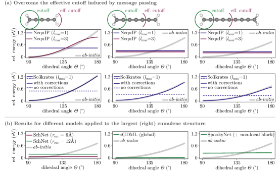
Figure 2: (a) Energy predictions for different cumulene structures with NequIP ($l_{\mathrm{max}}=1$ and $l_{\mathrm{max}}=3$) and So3krates ($l_{\mathrm{max}}=1$) models with and without geometric corrections (eqs. (13) and (14)). Cutoff radius and number of layers are kept constant at $r_{\mathrm{cut}}=2.5\,$\mathrm{\SIUnitSymbolAngstrom}$$ and $n_{l}=4$, respectively. (b) We additionally test other SOTA models on the largest cumulene structure (9 carbons). We find, that even for a very large cutoff, SchNet fails to describe the dihedral angle profile. The same holds true for an inherently global sGDML model and even for a SpookyNet model that explicitly includes non-local corrections.

As a representative example for MPNNs, we consider the recently proposed NequIP model [32], which achieves SOTA performance on several benchmarks. We find that even when the effective cutoff radius is large enough in principle, an MPNN with $n_{l}=4$, $r_{\mathrm{cut}}=2.5\,$\mathrm{\SIUnitSymbolAngstrom}$$, and $l_{\mathrm{max}}\leq 1$ fails to learn the correct energy profile. This is due to the fact that the relevant geometric information “cancels out” (similar to addition of vectors oriented in opposite directions) within each neighborhood, underlining the limited expressiveness of mean-field interactions in MPNNs. Only by including higher-order geometric correlations, e.g. going to $l_{\mathrm{max}}=3$, the correct energy profile can be recovered (at the cost of computational efficiency). When going to even larger cumulene structures, however, the effective cutoff becomes too small and it is necessary to increase the number of MP layers to solve the task (again, at the cost of lower computational efficiency), which is illustrated in appendix A.11. Neither increasing the maximum degree of interactions $l_{\mathrm{max}}$, nor the number of layers $n_{l}$, is a satisfactory workaround: Instead of offering a general solution to describe non-local interactions, both options decrease computational efficiency, while only shifting the problem to larger length-scales or higher-order geometric correlations.

We further apply three additional models to the cumulene structure with nine carbon atoms. To that end, we use an invariant SchNet model with varying cutoff distances (6 $\mathrm{\SIUnitSymbolAngstrom}$ and 12 $\mathrm{\SIUnitSymbolAngstrom}$), an inherently global but invariant sGDML model and the SpookyNet architecture which explicitly includes global effects using a non-local block. We find that none of the three is capable of describing the rotor energy profile of cumulene.

In contrast, our proposed So3krates architecture is able to reproduce the energy profile for cumulene molecules of all sizes independent of the effective cutoff radius. Crucially, even with $l_{\mathrm{max}}=1$, the predicted energy matches the ab-initio reference faithfully. We find that geometric corrections in the MP update of the SPHCs (cf. eq. (14)) are responsible for the increased capability of describing higher-order geometric correlations, as a So3krates model with a naive MP update (cf. eq. (13)) fails to solve this task with $l_{\mathrm{max}}=1$ (see Fig. 2a). We further confirm that the model picks up on the physically relevant interaction between the hydrogen rotors by analysing the attention values after training (see Fig. 8 appendix A.7). To illustrate how So3krates is able to describe non-local effects, we show a low-dimensional projection of the atomic SPHCs before and after training for the largest of the cumulene molecules (Fig. 3). After training, the SPHCs for hydrogen atoms at opposite ends of the molecule are embedded close together in SPHC space, allowing So3krates to efficiently model the non-local geometric dependence between the hydrogen rotors.

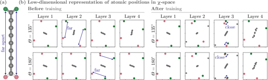
Figure 3: (a) Cumulene structure in Euclidean space. (b) Low-dimensional projections of the SPHCs ($l_{\mathrm{max}}=1$) in So3krates before and after training. Carbon atoms are grey and hydrogen atoms on different ends of the molecule are green and red, respectively. During training, the model maps hydrogen atoms at opposite ends close together in SPHC space (which is not the case at initialization).

Generalization to structures, larger than those in the training data are usually associated with the re-usability of the learned, local representations. For that reason, it is unclear if this property still holds when non-local corrections are used. As we show in appendix A.5 a So3krates model with non-local corrections still generalizes well to completely unknown and larger structures.

Benchmarks, Data Efficiency and Generalization

As pointed out in [31] and [32], equivariant features not only increase performance, but also improve data efficiency. The latter is particularly important, as ab-initio methods for reference data generation can become exceedingly expensive when high accuracy is required. Here, we use a subset of the recently introduced QM7-X data set [51], which we call QM7-X250. It contains 250 different molecular structures, each with 80 data points for training, 10 data points for validation and 11-3748 data points for testing (for details, see appendix A.9). The small number of training/validation samples per molecule makes it particularly suited for evaluating model behavior in the low data regime. In the following, we train (1) one model per structure in QM7-X250 and (2) one model for all structures in QM7-X250 ($250\times 80=20$k training points), which we refer to as individual and joint models, respectively.

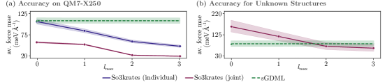
Figure 4: (a) Average force MAE as a function of $l_{\mathrm{max}}$ on 250 structures from QM7-X [51]. The blue solid line corresponds to So3krates models trained on each of the 250 structures (à 80 training points), individually. The jointly trained So3krates model (red solid line) is a single model trained on all $250\times 80$ training points. (b) Accuracy of force predictions for unknown structures as function of $l_{\mathrm{max}}$. Generalization is only investigated for the jointly trained model. Due to the way the molecular descriptor is designed, sGDML [38] models can only be trained on individual structures.

We start by investigating the performance as a function of the maximal degree $l_{\mathrm{max}}$ and find that the error strongly decreases with higher $l_{\mathrm{max}}$ (Fig. 4a). As kernel methods are known to perform well in the low-data regime [21], we compare our results to sGDML [38] kernel models, which only use distances as a molecular descriptor (corresponding to $l_{\mathrm{max}}=0$). For $l_{\mathrm{max}}=0$, we find sGDML gives competitive results, whereas for $l_{\mathrm{max}}=1$, So3krates starts to outperform sGDML. As soon as $l_{\mathrm{max}}\geq 2$, however, the prediction accuracy of So3krates is greater than that of sGDML by a large margin. Thus, increasing the order of geometric information in the SPHCs leads to strong improvements in the low-data regime. For jointly trained models, we find that So3krates outperforms sGDML even for $l_{\mathrm{max}}=0$, with continuous improvement for increasing $l_{\mathrm{max}}$. In appendix A.10 we report energy and force errors across degrees and further experimental details.

The generalization capability of So3krates is tested, by applying a jointly trained model to 25 completely unknown molecules from the QM7-X data set (see, Fig. 4b, details in appendix A.10). Again, we find that force MAEs decrease with increasing $l_{\mathrm{max}}$. For reference, we compare So3krates to individually trained sGDML models and find that So3krates performs on par, or even slightly better, for $l_{\mathrm{max}}\geq 2$. Going beyond $l_{\mathrm{max}}=2$ is found to only marginally improve generalization. In addition, we report results for a model trained on the full QM7-X data set in appendix A.5, following [30].

For completeness, we also apply So3krates to the popular MD17 benchmark (see Table 1). We find, that So3krates outperforms networks that have the same parameter complexity by a large margin (PaiNN and NewtonNet). Notably, it requires significantly less parameters than other SH based architectures (NequIP and SpookyNet), while performing only slightly worse or even on par with them. Furthermore, So3krates outperforms DimeNet, its closest competitor in timing (cf. Fig. 1.d), consistently by a large margin. Compared to current SH based approaches, GemNetQ needs less parameters (still $\sim 2.5$x more than So3krates) to achieve competitive results. However, it requires the explicit calculation of dihedral angles which scales cubically in the number of neighboring atoms. Due to its linear scaling (see A.8) and lightweight structure, So3krates can significantly reduce the time for training and inference (see Fig. 1d and A.6).

		NequIP [32] 3M | $\mathcal{O}(m)$	SpookyNet [30] 3M | $\mathcal{O}(m)$	GemNetQ [34] 2.2M | $\mathcal{O}(m^{3})$	DimeNet [29] 1.9M | $\mathcal{O}(m^{2})$	PaiNN [31] 600k | $\mathcal{O}(m)$	NewtonNet [52] 500k | $\mathcal{O}(m)$	So3krates 700k | $\mathcal{O}(m)$
Aspirin	energy forces	0.13 0.19	0.151 0.258	– 0.217	0.204 0.499	0.159 0.371	0.168 0.348	0.139 0.236
Ethanol	energy forces	0.05 0.09	0.052 0.094	– 0.088	0.064 0.230	0.063 0.230	0.061 0.211	0.052 0.096
Malondialdehyde	energy forces	0.08 0.13	0.079 0.167	– 0.159	0.104 0.383	0.091 0.319	0.096 0.323	0.077 0.147
Naphthalene	energy forces	0.11 0.04	0.116 0.089	– 0.051	0.122 0.215	0.117 0.083	0.118 0.084	0.115 0.074
Salicyclic Acid	energy forces	0.11 0.09	0.114 0.180	– 0.124	0.134 0.374	0.114 0.209	0.115 0.197	0.106 0.145
Toluene	energy forces	0.09 0.05	0.094 0.087	– 0.060	0.102 0.216	0.097 0.102	0.094 0.088	0.095 0.073
Uracil	energy forces	0.10 0.08	0.105 0.119	– 0.104	0.115 0.301	0.104 0.140	0.107 0.149	0.103 0.111

Table 1: MAE for energy (in kcal mol^-1) and forces (in kcal mol${}^{-1}\,$\mathrm{\SIUnitSymbolAngstrom}$^{-1}$) of current state-of-the-art machine learning models on the MD17 benchmark for 1k training points. For each model, the number of paramaeters, as well as the scaling in the number of neighbors $m$ is shown.

5 Discussion and Conclusion

Due to the locality assumption used in most MPNNs, they are unable to model non-local electronic effects, which result in global geometric dependencies between different parts of a molecule. The length-scales of such interactions often greatly exceed the cutoff radius used in the MP step, and even though stacking multiple MP layers increases the effective cutoff, ultimately, MPNNs are not capable of efficiently modeling geometric dependencies on arbitrary length scales.

In this work, we contribute conceptually by proposing an efficient and scalable solution to this problem. We suggest a set of refinable, equivariant coordinates for point clouds in Euclidean space, called spherical harmonic coordinates (SPHCs). Non-local geometric effects can then be efficiently modeled by including geometric corrections, which are localized in the space of SPHCs, but non-local in Euclidean space. Further, we show that introducing spherical filter functions acting on the SPHCs increases geometric resolution and predictive accuracy.

We then propose the So3krates architecture, a self-attention based MPNN, which decouples atomic features from higher-order geometric information. This allows to drastically decrease the parametric complexity while still achieving SOTA prediction accuracy. We show evidence that increasing the geometric order of SPHCs greatly improves model performance in the low-data regime, as well as generalization to unknown molecules.

A limitation of the current implementation of So3krates is that spherical neighborhoods $\mathcal{N}_{\bm{\chi}}$ in eq. (14) are computed from all pairwise distances in SPHC space. An alternative implementation could use a space partitioning scheme to find neighborhoods more efficiently. In a broader context, our work falls into the category of approaches that can help to reduce the vast computational complexity of molecular and material simulations. This can accelerate novel drug and material designs, which holds the promise of tackling societal challenges, such as climate change and sustainable energy supply [53]. Of course, our method could also be used for nefarious applications, e.g. design of chemical warfare, but this is true for all quantum chemistry methods.

Future research will focus on applications of So3krates to materials and bio-molecules, which are typical examples of chemical systems where the accurate description of non-local effects is necessary to produce novel insights. Efficient treatment of non-local effects in point cloud data goes beyond the domain of quantum chemistry. One way of representing non-local dependencies are non-local neural networks [54]. In comparison to the presented approach they compute a relation in feature rather than in Euclidean space, making it incapable of capturing direct geometric relations in Euclidean space. However, this might be necessary if the relative orientation of objects far apart from each other plays a role for identifying different objects.

6 Acknowledgements

All authors acknowledge support by the Federal Ministry of Education and Research (BMBF) for BIFOLD (01IS18037A). KRM was partly supported by the Institute of Information & Communications Technology Planning & Evaluation (IITP) grants funded by the Korea government(MSIT) (No. 2019-0-00079, Artificial Intelligence Graduate School Program, Korea University and No. 2022-0-00984, Development of Artificial Intelligence Technology for Personalized Plug-and-Play Explanation and Verification of Explanation), and was partly supported by the German Ministry for Education and Research (BMBF) under Grants 01IS14013A-E, AIMM, 01GQ1115, 01GQ0850, 01IS18025A and 01IS18037A; the German Research Foundation (DFG). We thank Stefan Chmiela, Mihail Bogojeski and Nicklas Schmitz for helpful discussions and feedback on the manuscript.

1. For all authors…

   1. Do the main claims made in the abstract and introduction accurately reflect the paper’s contributions and scope? [Yes]

   2. Did you describe the limitations of your work? [Yes]

   3. Did you discuss any potential negative societal impacts of your work? [Yes]

   4. Have you read the ethics review guidelines and ensured that your paper conforms to them? [Yes]

2. If you are including theoretical results…

   1. Did you state the full set of assumptions of all theoretical results? [N/A] We did not include theoretical results.

   2. Did you include complete proofs of all theoretical results? [N/A] Even though we proof equivariance, this is not a theoretical result of the presented work, as equivariance w. r. t. $\mathrm{SO(3)}$ is well understood.

3. If you ran experiments…

   1. Did you include the code, data, and instructions needed to reproduce the main experimental results (either in the supplemental material or as a URL)? [Yes]

   2. Did you specify all the training details (e.g., data splits, hyperparameters, how they were chosen)? [Yes]

   3. Did you report error bars (e.g., with respect to the random seed after running experiments multiple times)? [Yes] See Fig. 4 or Fig. 6.

   4. Did you include the total amount of compute and the type of resources used (e.g., type of GPUs, internal cluster, or cloud provider)? [Yes]

4. If you are using existing assets (e.g., code, data, models) or curating/releasing new assets…

   1. If your work uses existing assets, did you cite the creators? [Yes]

   2. Did you mention the license of the assets? [Yes]

   3. Did you include any new assets either in the supplemental material or as a URL? [Yes]

   4. Did you discuss whether and how consent was obtained from people whose data you’re using/curating? [N/A] No such data is used.

   5. Did you discuss whether the data you are using/curating contains personally identifiable information or offensive content? [N/A] No such data is used.

5. If you used crowdsourcing or conducted research with human subjects…

   1. Did you include the full text of instructions given to participants and screenshots, if applicable? [N/A] Neither crowdsourcing nor research on human subjects was conducted.

   2. Did you describe any potential participant risks, with links to Institutional Review Board (IRB) approvals, if applicable? [N/A] Neither crowdsourcing nor research on human subjects was conducted.

   3. Did you include the estimated hourly wage paid to participants and the total amount spent on participant compensation? [N/A] Neither crowdsourcing nor research on human subjects was conducted.

Appendix A Appendix

A.1 Proof of Equivariance

SPHC Initialization

Here we give proof that certain quantities from the main text are invariant or equivariant, respectively. Let us start with the spherical harmonic coordinates (SPHC) which are initialized as

$$\bm{\chi}_{i}^{(l)}(R)=\frac{1}{\mathcal{C}_{i}}\sum_{j\in\mathcal{N}(i)}\phi_{r_{\mathrm{cut}}}(r_{ij})\cdot\bm{Y}^{(l)}(\hat{\bm{r}}_{ij})\,,$$ (20)

where $\bm{Y}^{(l)}:S^{2}\mapsto\mathbb{R}^{2l+1}$. In contrast to the main text, we make the dependence of the right hand side of eq. (20) on the atomic positions $\mathcal{R}=\{\bm{r}_{1},\dots,\bm{r}_{n}\}$ explicit. Each degree-wise entry in the initialized SPHCs (eq. (20)) transforms under rotation as

$$\begin{split}\bm{\chi}_{i}^{(l)}(R_{\theta}\,\mathcal{R})&\sim\sum_{j\in\mathcal{N}(i)}\phi_{r_{\mathrm{cut}}}(r_{ij})\cdot\bm{Y}^{(l)}(R_{\theta}\hat{\bm{r}}_{ij})\\ &=\sum_{j\in\mathcal{N}(i)}\phi_{r_{\mathrm{cut}}}(r_{ij})\cdot\bm{D}^{l}(R_{\theta})\,\bm{Y}^{(l)}(\hat{\bm{r}}_{ij})\\ &=\bm{D}^{l}(R_{\theta})\,\sum_{j\in\mathcal{N}(i)}\phi_{r_{\mathrm{cut}}}(r_{ij})\cdot\bm{Y}^{(l)}(\hat{\bm{r}}_{ij})\\ &=\bm{D}^{l}(R_{\theta})\,\bm{\chi}_{i}^{(l)}(\mathcal{R})\,,\end{split}$$ (21)

where $\bm{D}(R_{\theta})^{l}\in\mathbb{R}^{(2l+1)\times(2l+1)}$ is the Wigner-D matrix for degree $l$ given rotation $R_{\theta}$ and $R_{\theta}\mathcal{R}=\{R_{\theta}\bm{r}_{1},\dots,R_{\theta}\bm{r}_{n}\}$. Since the cutoff function $\phi_{r_{\mathrm{cut}}}$ takes the inter-atomic distance $r_{ij}=\lVert\bm{r}_{j}-\bm{r}_{i}\rVert_{2}$ as its input argument it is always invariant under rotation. Thus, each degree-wise entry $\bm{\chi}^{(l)}$ is equivariant after the initialization.

SPHC Message Passing Update

After initialization, each per-degree entry in $\bm{\chi}$ is updated as

$$\bm{\chi}_{i}^{\prime\,(l)}(\mathcal{R})=\bm{\chi}_{i}^{(l)}(\mathcal{R})+\sum_{j\in\mathcal{N}(i)}\phi_{r_{\mathrm{cut}}}(r_{ij})\cdot\alpha^{(l)}_{ij}\cdot\bm{Y}^{(l)}(\hat{\bm{r}}_{ij})\,,$$ (22)

where $\alpha^{(l)}_{ij}$ are rotationally invariant, per-degree self-attention coefficients. In the first layer, the first part in eq. (22) corresponds to the initialized SPHC entries, which have been already shown to be equivariant (see above). The second part of the equation has the same structural form as the initialization, with the additional self-attention value, which is a rotationally invariant scalar. Thus we can write

$$\begin{split}\bm{\chi}_{i}^{\prime\,(l)}(R_{\theta}\,\mathcal{R})&=\bm{D}^{l}(R_{\theta})\,\bm{\chi}^{(l)}(\mathcal{R})+\sum_{j\in\mathcal{N}(i)}\phi_{r_{\mathrm{cut}}}(r_{ij})\cdot\alpha^{(l)}_{ij}\cdot\bm{Y}^{(l)}(R_{\theta}\hat{\bm{r}}_{ij})\\ &=\bm{D}^{l}(R_{\theta})\,\bm{\chi}^{(l)}(\mathcal{R})+\bm{D}^{l}(R_{\theta})\,\sum_{j\in\mathcal{N}(i)}\phi_{r_{\mathrm{cut}}}(r_{ij})\cdot\alpha^{(l)}_{ij}\cdot\bm{Y}^{(l)}(\hat{\bm{r}}_{ij})\\ &=\bm{D}^{l}(R_{\theta})\,\bigg{(}\bm{\chi}_{i}^{(l)}(\mathcal{R})+\sum_{j\in\mathcal{N}(i)}\phi_{r_{\mathrm{cut}}}(r_{ij})\cdot\alpha^{(l)}_{ij}\cdot\bm{Y}^{(l)}(\hat{\bm{r}}_{ij})\bigg{)}\\ &=\bm{D}^{l}(R_{\theta})\,\bm{\chi}_{i}^{\prime\,(l)}(\mathcal{R})\,,\end{split}$$ (23)

which shows that the updated $\bm{\chi}^{\prime\,(l)}$ is also equivariant. The proof of equivariance for later layers follows analogously.

Transformation of the SPHCs

After having shown that each per-degree entry of $\bm{\chi}$ transforms under rotation according to the corresponding Wigner-D matrix $\mathbf{D}^{l}(R_{\theta})\in\mathbb{R}^{(2l+1)\times(2l+1)}$, one can write the direct sum of all Wigner-D matrices as concatenation of matrices along the diagonal

$$\bm{D}(R_{\theta})=\bigoplus_{l\in\mathcal{L}}\bm{D}^{l}(R_{\theta})\,,$$ (24)

such that $\bm{D}(R_{\theta})\in\mathbb{R}^{(l_{\mathrm{max}}-l_{\mathrm{min}}+1)\times(l_{\mathrm{max}}-l_{\mathrm{min}}+1)}$ has a block diagonal structure. The, full SPHC vectors transform under rotation as

$$\bm{D}(R_{\theta})\,\bm{\chi}(\mathcal{R})=[\bm{D}^{l_{\mathrm{min}}}(R_{\theta})\bm{\chi}^{(l_{\mathrm{min}})}(\mathcal{R}),\dots,\bm{D}^{l_{\mathrm{max}}}(R_{\theta})\bm{\chi}^{(l_{\mathrm{max}})}(\mathcal{R})]\,.$$ (25)

As each of the blocks along the diagonal of $\bm{D}(R_{\theta})$ is an orthogonal Wigner-D matrix, $\bm{D}(R_{\theta})$ itself is also orthogonal.

A.1.1 Invariance of the (per-degree) Norm

The per degree norm is used as input to the spherical filter function $\phi_{s}$. As shown above, each of the per-degree entries in $\bm{\chi}$ transforms under rotation as

$$\bm{\chi}^{(l)}(R_{\theta}\,\mathcal{R})=\bm{D}^{l}(R_{\theta})\bm{\chi}^{(l)}(\mathcal{R})\,.$$ (26)

The squared norm can be expressed in terms of an inner product

$$\begin{split}\lVert\bm{\chi}^{(l)}(R_{\theta}\mathcal{R})\rVert_{2}^{2}&=\big{(}\bm{\chi}^{(l)}(R_{\theta}\,\mathcal{R})\big{)}^{T}\,\bm{\chi}^{(l)}(R_{\theta}\,\mathcal{R})\\ &=(\bm{D}^{l}(R_{\theta})\,\bm{\chi}^{(l)}(\mathcal{R}))^{T}\,(\bm{D}^{l}(R_{\theta})\,\bm{\chi}^{(l)}(\mathcal{R}))\\ &=\big{(}\bm{\chi}^{(l)}(\mathcal{R})\big{)}^{T}\underbrace{\big{(}\bm{D}^{l}(R_{\theta})\big{)}^{T}\,\bm{D}^{l}(R_{\theta})}_{=\mathbb{I}}\,\bm{\chi}^{(l)}(\mathcal{R})\\ &=\lVert\bm{\chi}^{(l)}(\mathcal{R})\rVert_{2}^{2},\end{split}$$ (27)

where we use the orthogonality of Wigner-D matrices to show that the inner product is rotationally invariant. If $\lVert\cdot\rVert_{2}^{2}$ is invariant, so is $\lVert\cdot\rVert_{2}$, which completes the proof of equivariance for the degree-wise norm.

The squared norm of the full SPHC vector $\bm{\chi}$ transforms under rotation as

$$\begin{split}\lVert\bm{\chi}(R_{\theta}\,\mathcal{R})\rVert_{2}^{2}&=\big{(}\bm{\chi}(R_{\theta}\,\mathcal{R})\big{)}^{T}\bm{\chi}(R_{\theta}\,\mathcal{R})\\ &=\big{(}\bm{D}(R_{\theta})\bm{\chi}(\mathcal{R})\big{)}^{T}\big{(}\bm{D}(R_{\theta})\bm{\chi}(\mathcal{R})\big{)}\\ &=\big{(}\bm{\chi}(\mathcal{R})\big{)}^{T}\underbrace{\big{(}\bm{D}(R_{\theta})\big{)}^{T}\,\bm{D}(R_{\theta})}_{=\mathbb{I}}\,\bm{\chi}(\mathcal{R})\\ &=\lVert\bm{\chi}(\mathcal{R})\rVert_{2}^{2}\,,\end{split}$$ (28)

where we used that the orthogonality of $\bm{D}^{l}$ results in orthogonality of $\bm{D}$ (as argued above).

A.2 Spherical Neighborhood

Starting point for the construction of the spherical neighborhood are the SPHCs $\mathcal{X}$ in a given layer of So3krates. Consequently, the distance matrix in SPHC for all atomic pairs is given as an $n\times n$ matrix $\bm{X}$ with entries $\chi_{ij}=\lVert\bm{\chi}_{i}-\bm{\chi}_{j}\rVert_{2}$. The idea of a spherical neighborhood is to only consider atoms that lie within a certain distance w. r. t. each other in SPHC space, meaning only those for which $\chi_{ij}\leq\chi_{\text{cut}}$ holds. However, compared to the inter-atomic distances in Euclidean space, for which specific knowledge e.g. about bond lengths or interaction length scales exits, this is not the case for the rather abstract space of SPHCs. Thus, we apply a softmax function along each row (neighborhood) of $\bm{X}$, which gives a rescaled version of the spherical distance matrix $\tilde{\bm{X}}$ with rescaled entries $\tilde{\chi}_{ij}\in(0,1)$. Neighborhoods for each atom are then selected based on a polynomial cutoff function [29]

$$\phi_{\chi_{\text{cut}}}(x)=1-\frac{(p+1)(p+2)}{2}x^{p}+p(p+2)x^{p+1}-\frac{p(p+1)}{2}x^{p+2},$$ (29)

where the input is given as $x=\tilde{\chi}_{ij}/\chi_{\text{cut}}$. Here we chose $\chi_{\text{cut}}=\kappa/n$, where $n$ is the number of atoms in the system and $\kappa$ allows to increase or decrease the size of the cutoff radius. By scaling with the inverse of the number of atoms in the system, we ensure that the relative number of neighboring atoms remains approximately constant, even when going to larger molecules. The parameter $\kappa$ allows to fine tune the relative number of atoms and can depended on the size and type of the molecule under investigation. For our cumulene experiments we chose $\kappa=1$ and $p=6$, which reduces the number of considered interactions by $\sim 40\%$ compared to a global model.

A.3 Network Architecture

The So3krates model is available at https://github.com/thorben-frank/mlff. It makes extensive use of the libraries Flax [55] for building the networks, Optax [56] for training and Numpy [57] and Jax [58] for additional processing steps. All code and data that is necessary to produce the results step by step presented in the main body of the paper can be downloaded from https://zenodo.org/record/6584855 (newest version).

Detailed Network Design

We now describe the specific implementation of the building blocks that we have formally introduced in the main text. The computational flow of the architecture is shown in Fig. 5.

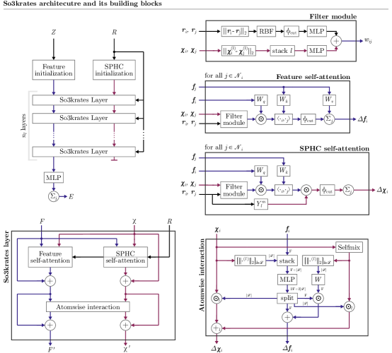
Figure 5: Figure shows the architecture of So3krates and its individual building blocks. More details about the different modules can be found in the corresponding sections in A.3. Here $[\lVert\cdot_{l}\rVert_{2}]_{l\in\mathcal{L}}$ denotes per-degree norm followed by concatenation. The subscript $l$ at the pointwise product and the addition (in the atomwise interaction module) illustrates that each degree is multiplied with one entry of the $|\mathcal{L}|$-sized output vector.

Radial Filter

For the radial filter function $\phi_{r}:\mathbb{R}\mapsto\mathbb{R}^{F}$ (first summand in eq. (16)) the interatomic distances are expanded in terms of $K$ radial basis functions as proposed in PhysNet [19], which are given as

$$\theta^{k}(r_{ij})=\phi_{r_{\mathrm{cut}}}(r_{ij})\,\cdot\,\exp{\big{(}-\gamma(\exp{(-r_{ij}})-\mu_{k})^{2}\big{)}},$$ (30)

where $\mu_{k}$ is the center of the $k$-th basis function ($k=1\dots K$). The cutoff function

$$\phi_{r_{\mathrm{cut}}}(r_{ij})=\frac{1}{2}\left(\cos\left(\frac{\pi r_{ij}}{r_{\mathrm{cut}}}\right)+1\right)$$ (31)

guarantees that $\theta^{k}(r_{ij})=0$ smoothly goes to zero when interatomic distances exceed the cutoff radius $r_{\mathrm{cut}}$. Here we chose $K=32$ basis functions in total. The expanded distance is passed in a two-layered MLP with silu non-linearity in-between and $128$ hidden and $F$ output neurons, respectively.

Spherical Filter

The spherical filter function $\phi_{s}\left([\chi^{(l)}_{ij}]_{l\in\mathcal{L}}\right):\mathbb{R}^{|\mathcal{L}|}\mapsto\mathbb{R}^{F}$ (second summand in eq. (16)) is also modelled as a two-layered MLP with the same non-linearity. Its input is given as the stacked per-degree distances $\chi_{ij}^{(l)}$, such that the input to the MLP is of low dimension (number of spherical degrees $l$). For that reason, we only use 32 neurons in the first and again $F$ neurons in the second layer.

Self-Attention

The self-attention matrix (cf. eq. (15)) is calculated from the filter vector $w_{ij}$ as well as from a pair of feature vectors $\bm{f}_{i}\in\mathbb{R}^{F}$ and $\bm{f}_{j}\in\mathbb{R}^{F}$. Before being passed to the inner product, each of the feature vectors is refined using a linear layer which we denote as $W_{q}$ and $W_{k}$ in the fashion of the key and query matrices usually appearing in the calculation of self-attention coefficients [49]. Thus, the self-attention coefficients are calculated as

$$\alpha_{ij}=\frac{1}{\sqrt{F}}\,\bm{q}_{i}^{T}(\bm{w}_{ij}\odot\bm{k}_{j}),$$ (32)

where $\bm{q}_{i}=W_{q}{f}_{i}\in\mathbb{R}^{F}$, $\bm{k}_{j}=W_{k}\bm{f}_{j}\in\mathbb{R}^{F}$ and $\bm{w}_{ij}\in\mathbb{R}^{F}$ comes from the filter module. The features $\bm{f}_{j}$ of the neighboring atoms are also passed through an additional linear layer $W_{v}$. The updated features are then given as

$$\bm{f}_{i}^{\prime}=\bm{f}_{i}+\sum_{j\in\mathcal{N}(i)}\phi_{r_{\mathrm{cut}}}(r_{ij})\cdot\alpha_{ij}\cdot(W_{v}\bm{f}_{j})$$ (33)

and the updates to the SPHCs as

$$\bm{\chi}_{i}^{\prime\,(l)}=\bm{\chi}_{i}^{(l)}+\sum_{j\in\mathcal{N}(i)}\phi_{r_{\mathrm{cut}}}(r_{ij})\cdot\alpha_{ij}^{(l)}\cdot\bm{Y}^{(l)}(\bm{r}_{ij})\,.$$ (34)

Different parameters are used for the feature and SPHC updates, respectively. For the feature update, we use a predefined number of heads whereas the number of heads in the SPHC update equals the number of degrees in the SPHC vector. In order to ensure permutation invariance, all parameters of the linear layers are shared across atoms.

Atomwise Interaction

After the update MP step, we update the features as well as the SPHCs per atom. In this step, we do not only include cross-degree coupling in $\bm{\chi}$ but also allow for information exchange between the feature and the SPHC branch. The functions $\phi_{1}\left(\mathbf{f}_{i},[\chi_{i}^{(l)}]_{l\in\mathcal{L}},[\tilde{\chi}_{i}^{(l)}]_{l\in\mathcal{L}}\right)$ and $\phi_{2}^{(l)}\left(\mathbf{f}_{i},[\chi_{i}^{(l)}]_{l\in\mathcal{L}},[\tilde{\chi}_{i}^{(l)}]_{l\in\mathcal{L}}\right)$ are implemented by a shared MLP. The function $\phi_{3}^{(l)}\left([\tilde{\chi}_{i}^{(l)}]_{l\in\mathcal{L}}\right)$ is implemented by a single linear layer, without bias term. The full computational flow is shown in Fig. 5.

A.4 Ablation Study Spherical Filter

To illustrate the importance of the spherical filter, we examine its effect in an ablation study on the MD17 benchmark for varying maximal degree $l_{\mathrm{max}}$. As can be seen in Fig. 6, using spherical filters (see eq. (16)) improves performance compared to a So3krates model without them (solid vs. dotted lines), where the difference becomes even more pronounced for force predictions.

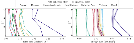
Figure 6: Ablation study on MD17 for using spherical filters. The model is evaluated on five different splits (a 1k points) of the data, where the transparent envelope is the $2\sigma$ confidence interval.

Further, the effect of spherical filters becomes stronger for smaller $l_{\mathrm{max}}$. Since many equivariant MPNNs carry features including additional channels for higher order geometric information, spherical filters can be straight forwardly integrated into current architectures, offering the potential of increased accuracy.

A.5 QM7-X Experiments

As an additional benchmark, we train So3krates on the full QM7-X data set and compare our results to the reported errors for known and unknown molecules in table 2. The known molecules correspond to the test samples that have not been seen during training. Following [30], we use the keys (idmol in the QM7-X data base) [1771, 1805, 1824, 2020, 2085, 2117, 3019, 3108, 3190, 3217, 3257, 3329, 3531, 4010, 4181, 4319, 4713, 5174, 5370, 5580, 5891, 6315, 6583, 6809, 7020] for testing the generalization of our model to unknown structures, which have been excluded from the data set prior to generating train, test and validation splits.

		SchNet [13]	PaiNN [31]	SpookyNet [30]	So3krates $F=132$	So3krates $F=264$	So3krates + non local
known molecules / unknown conformations	Energy Forces	50.847 53.695	15.691 20.301	10.620 14.851	16.815 20.422	15.228 18.446	16.176 19.879
unknown molecules / unknown conformations	Energy Forces	51.275 62.770	17.594 24.161	13.151 17.326	21.733 25.211	21.750 23.169	20.071 24.236

Table 2: Energy and force MAEs in meV and meV $$\mathrm{\SIUnitSymbolAngstrom}$^{-1}$ for different models trained on the full QM7-X data set.

Accuracy Comparison Local vs. Non-Local Model

By comparing the results reported in table 2 we find, that the non-local model shows the same accuracy as the local model for both known and unknown molecules. This underlines the applicability of the presented, non-local corrections to a large variety of molecular structures including transfer learning to unknown molecules.

Accuracy Improvement by Up-Scaling

Despite the parametric leightweight structure of So3krates, it is important that results can be imrproved by upscaling the model. Here we take one of the most straight forward paths and upscale the model by simply increasing the feature dimension from $F=132$ to $F=164$. As it can be seen in table 2, this already allows to increase the accuracy on the QM7-X dataset compared to the base line model. It should be noted, however, that one could follow additional/other directions, such as increasing the maximal degree $l_{\mathrm{max}}$.

Generalization to Larger Molecules with a Non-Local Model

As seen in table 2, a model with non-local correction is capable of generalizing to structures not seen during training. However, the re-usability of local information is one of the key assumptions for building models that can be trained on small molecules and afterwards be applied to larger, completely unknown structures [30]. Thus, testing the non-local model on unknwon structures from the QM7-X data set is an insufficient test to investigate this property of transfer learning. We therefore use the non-local model for geometry optimization of molecules that range from 47 (riboflavin) up to 109 atoms (Ala10) in size (see 7).

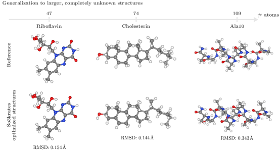
Figure 7: The upper row shows the optimized reference geometry obtained with PBE0-MBD calculation (taken from  [30]). The bottom row shows geometry optimized structures obtained with a So3krates model with non-local corrections from SPHC space as well as the root mean squared deviation from the reference structure. The model has been trained on the QM7-X data set for which the largest contained structure has 23 atoms. Thus, So3krates can generalize to larger, unknown structures without relying on the assumption of locality.

We find that the non-local model is robust for geometry optimization when being applied to much larger, unknown molecules. The largest molecule in the QM7-X data set has $23$ atoms.

A.6 Time Analysis

In order to determine the training and inference times, we follow [34] and evaluate our model on the toluene molecule from the MD17 benchmark with a batch size of 4. We trained a NequIP model with the same hyperparameters as reported in [32] as well as a So3krates model on a Tesla P100 with 12GB. The reported training time corresponds to the wall time it took each model to evaluate a single gradient update (without time for validation). We compare these runtimes to the runtimes that have been reported for DimeNet [29] and GemNetQ [34] in [34]. However, these reported times have been measured on a GeForce GTX 1080Ti (a GPU we did not have access to). In [37] it has been found that a Tesla P100 gives a speedup factor of $\sim 1.3$, such that we downscale the reported runtimes accordingly. The resulting times are shown in table 3, which are the values plotted in 1d. It should be noted, that our implementation did not focus on the runtime, such that it is likely to be possible to further reduce the computational cost that is required for training and inference.

	So3krates		NequIP [32]		DimeNet [29]		GemNetQ [34]
	training	inference	training	inference	training	inference	training	inference
time (ms)	34	12	507	136	218	24	483	76

Table 3: Training and inference times for different models for the toluene molecule from the MD17 benchmark and a batch size of 4. Hyperparemters for So3krates are the ones that have been used to produce the reported results on the MD17 benchmark (cf. Tab. 1). Times for DimeNet and GemNetQ have been measured on a different GPU, such that we decrease their runtimes by the factor reported here [37]. Inference times are for energy and force predictions.

A.7 Analysis of Attention Coefficients

In figure 8 we plot the attention coefficients from the MP update of the SPHCs (cf. eq. (14)) after training for different dihedral angles between the rotors. Attention values are calculated as the average over all attention values obtained for a given atomic pair throughout all SPHC update steps. As it can be verified visually, the model picks up physically important interactions. Care should be taken, however, since it has been pointed out in [59] that looking at the bare attention values only has limited expressiveness.

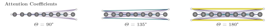
Figure 8: Visualization of the attention coefficients from the MP update of the SPHCs (cf. eq. (14)) for different dihedral angles between the rotors.

A.8 Scaling Analysis

We further compare the scaling of three different versions of the So3krates model. Namely, we compare a local So3krates model, which only localizes in $\mathbb{R}^{3}$ (used in 4.1), a non-local So3krates model with non-local corrections from SPHC space (used in 4.2) and a fully global model for which the cutoff radius is chosen such that all atoms are in each others neighborhood. The inference times for energy predictions for molecules ranging from 9 up to 370 atoms are shown in Fig. 9. As expected, we find linear scaling for the local So3krates version with a remarkable inference time of only $\sim 196$ ms for 370 atoms (batch size is 25). For the fully global mode, we see quadratic scaling in the number of atoms. The model with non-local corrections can be found somewhere in-between the local and the global model. To that end, we want to stretch the fact that we did not focus on an efficient implementation for the non-local corrections. The experiments were run on a Tesla P100 with 12 Gb and a batch size of 25.

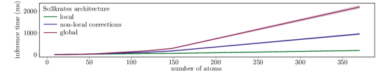
Figure 9: Scaling comparison between a local So3krates (as used in the first part of the experiment section 4.1), an architecture with non-local corrections (as used in the second part of the experiment section 4.2) and a global So3krates model (only used for the sake of comparison). As expected, the local model shows linear scaling in the number of atoms and only takes $\sim 196$ ms for a system with 370 atoms. We also find the model with non-local correction to balance between the quadratically scaling global model and the linear local model. Due to memory issues for the fully global model for larger structures, we only report inference times for energy predictions.

A.9 QM7-X250

As starting point for the recently introduced QM7-X dataset [51] serve $\sim 7$k molecular graphs with a maximum of 7 non-hydrogen atoms (C, N, O, S, Cl). By sampling and optimizing structural and constitutional isomers for each graph, $\sim 42$k equilibrium structures are generated. Using normal mode sampling at 1500 K, 100 out-of-equilibrium points are generated for each structure resulting in 101 data points per structure and $\sim 4.2$M geometries in total.

In order to make the data set well suited for both, kernel and neural network models, we group the geometries by structural isomers which gives $\sim 13$k individual data sets, each consisting of #stereo-isomers $\times 101$ geometries. For each of the data sets we choose 80 points for training, 10 points for validation and the remaining points for testing after the training. Afterwards, we randomly sample 250 data sets out of the 13k data sets. The comparison of the probabilities of drawing a molecule with a given number of atoms, number of symmetries and number of stereo-isomers from the original QM7-X and the QM7-X250 data sets are shown in Fig. 10. Since we ensure that each of the structural subsets present in the original data set is also present in the 250 drawn samples at least once, it can be seen that these structures are over represented in the QM7-X250 data set, even though they only make up a single structure. Apart from these special structures, we see that the sampled dataset correctly reproduces the distribution of the original data set.

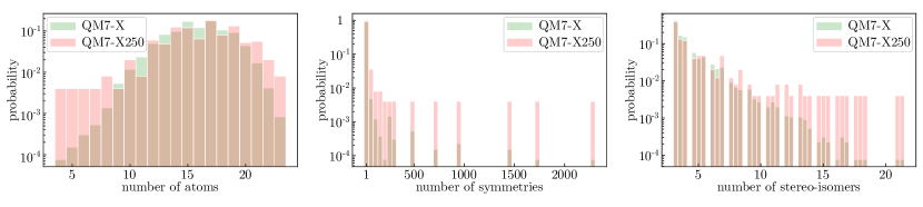
Figure 10: The figure shows the probability of occurrence for structures with a certain property value in the original QM7-X and the sub-sampled QM7-X250 dataset. As it can be seen, QM7-X follows the distribution of the original dataset. As for each property value at least once structure is present in QM7-X250 (per design), values with a low count in the original data set have higher relative importance, which can be seen e.g. for structures with only a few atoms, or with high symmetry.

From the 250 sampled structures, we build 250 per structure data sets with 80 training, 10 validation and 10–3748 (depending on the number of stereo-isomers) test points, which we referred to as individual dataset in the main text. We can further build a joint dataset, by merging all individual structures into a single data set, which gives 20 000 ($250\times 80$) training, 2 500 ($250\times 10$) validation, and 108 800 testing points.

A.10 QM7-X250 Experiments

In the main text we show the force MAE as a function of maximal order $l_{\mathrm{max}}$ in Fig. 4a. In table 4, we further show the exact errors for energy and forces as a function of maximal order $l_{\mathrm{max}}$, as well as the number of parameters per So3krates model. For all models with $l_{\mathrm{max}}\geq 1$, we do not include $l_{\mathrm{max}}=0$ within the SPHCs, since the zeroth degree evaluates to a constant one and thus does not contain any additional geometric information.

		sGDML [38]		So3krates $l_{\mathrm{max}}=0$		So3krates $l_{\mathrm{max}}=1$		So3krates $l_{\mathrm{max}}=2$		So3krates $l_{\mathrm{max}}=3$
		individual	joint	individual	joint	individual	joint	individual	joint	individual	joint
QM7-X250	energy forces	67.78 107.66	– –	78.40 105.80	46.87 57.57	66.43 84.54	44.64 52.58	47.02 59.33	19.10 27.77	38.40 48.46	17.09 25.37
# parameters		–		846k		846k		746k		716k

Table 4: Comparison of the averaged per structure MAE for energy (in meV) and forces (in meV $$\mathrm{\SIUnitSymbolAngstrom}$^{-1}$) for sGDML and So3krates models with varying $l_{\mathrm{max}}$. Best results are in bold. Note that for small $l_{\mathrm{max}}$ the total number of parameters decreases, since in the SPHC update step, as many heads are used as there are degrees (one degree for $l_{\mathrm{max}}=0$ and $l_{\mathrm{max}}=1$). As a consequence, the size of the matrices $Q$ and $K$, that are applied to the feature vectors that make up the inner product, become smaller in size. The feature dimension $F=132$ is the same for all models. This leads to a decrease of the total number of network parameters, which is larger than the increase in network parameters, due to the additional degrees. Note that it is important to take the average over per structure MAEs, since the different structures have differently many test samples (see section A.9).

The generalization to unknown molecules is tested on the same structure keys as in the SpookyNet paper [30] and in the QM7-X experiment from above A.5. As we only trained on forces and generalize to completely unknown molecules, we can not fit the energy integration constant (as we assume to have no reference data for the unknown molecules). For that reason we only report force errors (see 5).

		sGDML [38]	So3krates $l_{\mathrm{max}}=0$	So3krates $l_{\mathrm{max}}=1$	So3krates $l_{\mathrm{max}}=2$	So3krates $l_{\mathrm{max}}=3$
Generalization	forces	86.84	159.42	117.91	76.05	$\bm{68.29}$

Table 5: Comparison of the averaged per structure MAE for forces (in meV $$\mathrm{\SIUnitSymbolAngstrom}$^{-1}$) for sGDML and So3krates models with varying $l_{\mathrm{max}}$ when applied to completely unknown structures. Best results are in bold. Due to the way the molecular descriptor is designed, sGDML [38] models can only be trained on individual structures. Thus the reported results for sGDML are not generalization results but rather serve as a benchmark for the generalization MAE of So3krates. The number of parameters are the same as reported in Tab. 4. Note that it is important to take the average over per structure MAEs, since the different structures have differently many test samples (see section A.9).

However, one could train a So3krates model on both, energy and forces to obtain meaningful predictions for both. In that case, atomization energies would need to be included to obtain equal energy scales across different molecules as done for the full QM7-X data set.

A.11 Additional Experiments for Non-Local Effects

Here we demonstrate, that increasing the number of local MP steps in NequIP allows to model the non-local effects in cumulene, as an increase of the number of steps increases the effective cutoff of the model (see Fig. 11). However, this just shifts the problem to larger distances; increasing the length of the cumulene molecule again leads to a scenario where the local model fails.

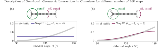
Figure 11: (a) Description of the energy profile in cumulene using $n_{l}=4$ in the NequIP model, such that the effective cutoff radius is smaller then the length scale on which the electronic effects take place. (b) By increasing the number of layers to $n_{l}=6$, the effective cutoff becomes large enough to transfer information about the rotor orientation along the molecular graph. However, the problem is only shifted to larger length scales.

A.12 Benchmarks for Non-Local Effects

We further apply So3krates to the benchmark presented in [60], which explicitly introduces structures which exhibit non-local effects. We find, that for the carbon chain with non-local charge transfer, So3krates with non-local corrections improves by a factor $\sim 2$ compared to a local model. For the remaining structures no such difference can be found. Notably, the non-local effects from the presented benchmark do not result in global geometric relations but rather change the overall behavior by adding or removing certain atoms (called doping). Thus, a combination of the So3krates mechanism (for geometric relations) and the mechanism presented in SpookyNet might be a valuable direction for future work. Full results are reported in table 6. Note that So3krates could be easily extended to predict partial charges as well following e.g. [30].

		2G-BPNN	3G-BPNN	4G-BPNN	SpookyNet	So3krates	So3krates + non local
C10H2 / C10H${}_{2}^{+}$	Energy Forces Charges	1.619 129.5 –	2.045 231.0 20.08	1.194 78.0 6.577	0.364 5.802 0.117	0.113 13.198 –	0.122 7.844 –
Na8/9Cl${}_{8}^{+}$	Energy Forces Charges	1.692 57.39 –	2.042 76.67 20.80	32.78 15.82 1.323	1.052 1.052 0.111	0.455 3.126 –	0.474 3.316 –
Au2-MgO	Energy Forces Charges	2.287 153.1 –	– – –	0.219 66.0 5.698	0.107 5.337 1.013	0.062 8.130 –	0.064 9.472 –

Table 6: RSME errors for energy and forces in meV / atom and meV / $\mathrm{\SIUnitSymbolAngstrom}$ for various generations of Behler-Parinello networks [60], SpookyNet [30] and a local and non-local So3krates model.

A.13 Training Details

We train So3krates by minimizing a combined loss of energy and forces

$$\text{Loss}=(1-\beta)\cdot(E-\tilde{E})^{2}+\frac{\beta}{3N}\sum_{k=1}^{n}\sum_{i\in(x,y,z)}(F_{k}^{i}-\tilde{F}_{k}^{i})^{2},$$ (35)

where $\tilde{E}$ and $\tilde{F}$ are the ground truth and $E$ and $F$ are the predictions of the model. The loss is evaluated on mini batches with a batch size given in table Tab. 7. The parameter $\beta$ is used to control the trade-off between energy and forces and additionally accounts for different energy and force scales. We train our models with the ADAM optimizer [61] and an initial learning rate of $\mu=1\times 10^{-3}$. We use exponential learning rate decay where the learning rate is decreased by a factor of $0.5$ every 1k epochs for the MD17 benchmark and the joint QM7-X250 dataset and every 300 epochs for individual models on the QM7-X250 dataset. For training on the full QM7-X data set we reduced the leraning rate every 250 epochs by a factor of 0.7. We further applied gradient clipping to a maximal norm of 1.

Additional hyperparameters that have been used to produce the tables and figures in this work are given Tab. 7. Whenever $\beta=1$ is reported, no energy contribution did enter the loss function. In that case, we calculated the integration constant for energy according to section A.14.

Ref.	$F$	$n_{\mathrm{layers}}$	$r_{\mathrm{cut}}$ ($\mathrm{\SIUnitSymbolAngstrom}$)	$l_{\mathrm{max}}$	geom. corr.	spherical filter	$\beta$	epochs	$B_{s}$	$N_{\mathrm{train}}$	$N_{\mathrm{valid}}$
Fig. 2	128	4	2.5	1	True/False	True	1	4k	8	1k	1k
Fig. 3	128	4	2.5	1	True/False	True	1	4k	8	1k	1k
Fig. 4a	132	6	5	[0,1,2,3]	False	True	1	1.5k	1	80	10
Fig. 4b	132	6	5	[0,1,2,3]	False	True	1	6k	100	20k	2.5k
Tab. 1	132	6	5	3	False	True	0.99	4k	8	1k	1k
Fig. 6	[128, 128, 132, 128]	6	5	[1,2,3,4]	False	True / False	0.99	4k	8	1k	1k
Fig. 7	132	6	5	3	True	True	0.99	1k	100	3.6M	360k
Tab. 2	132	6	5	3	True/False	True	0.99	1k	100	3.6M	360k
Tab. 2	264	6	5	3	False	True	0.99	1k	100	3.6M	360k
Tab. 6	132	6	5	3	True/False	True	0.99	1k	100	*	*

Table 7: Training hyperparameters: Table summarizes the training hyperparameters, used for the different models and experiments. Experiments are identified via their figure/table number in the main text. For the results reported in Tab. 6, the same sizes of data splits as reported in [60] have been used (indicated by an asterix).

A.14 Energy Integration Constant

When only training on forces, the resulting energy predictions are likely to be shifted w. r. t. the correct energy values, due to vanishing constants when taking the derivative. Since force fields are conservative vector fields, one can define the following loss for the constant $c$ as

$$\begin{split}\mathcal{L}(c)&=\sum_{i=1}^{M}\left(\int\mathbf{f}_{\mathrm{F}}(R_{i})\,\mathrm{d}R_{i}-E_{i}\right)^{2}\\ &=\sum_{i=1}^{N_{\mathrm{data}}}\left(f_{\mathrm{E}}(R_{i})+c-E_{i}\right)^{2}\end{split}$$ (36)

where index $i$ runs over the $M$ data points, $R_{i}\in\mathbb{R}^{n\times 3}$ are the atomic coordinates and $E_{i}$ is the reference value of the PES. The functions $\mathbf{f}_{\mathrm{F}}:\mathbb{R}^{n\times 3}\mapsto\mathbb{R}^{n\times 3}$ and $f_{\mathrm{E}}:\mathbb{R}^{n\times 3}\mapsto\mathbb{R}$ are the force and energy function, respectively. Minimization w. r. t. to $c$ then gives

$$\partial_{c}\,\mathcal{L}(c) \overset{!}{=}0$$ (37)

$$\iff 2\sum_{i=1}^{M}c-\big{(}E_{i}+f_{\mathrm{E}}(R_{i})\big{)} =0$$ (38)

$$\iff \frac{1}{M}\sum_{i=1}^{M}E_{i}+f_{\mathrm{E}}(R_{i}) =c\,.$$ (39)

Thus, the shifted energy function is given as $\tilde{f}_{\mathrm{E}}(R_{i})=c+f_{\mathrm{E}}(R_{i})$.