A New Semi-Structured Algebraic Multigrid Method

Abstract

Multigrid methods are well suited to large massively parallel computer architectures because they are mathematically optimal and display excellent parallelization properties. Since current architecture trends are favoring regular compute patterns to achieve high performance, the ability to express structure has become much more important. The hypre software library provides high-performance multigrid preconditioners and solvers through conceptual interfaces, including a semi-structured interface that describes matrices primarily in terms of stencils and logically structured grids. This paper presents a new semi-structured algebraic multigrid (SSAMG) method built on this interface. The numerical convergence and performance of a CPU implementation of this method are evaluated for a set of semi-structured problems. SSAMG achieves significantly better setup times than hypre’s unstructured AMG solvers and comparable convergence. In addition, the new method is capable of solving more complex problems than hypre’s structured solvers.

65F08, 65F10, 65N55

1 Introduction

The solution of partial differential equations (PDEs) often involves solving linear systems of equations

(1) $$A\mathbf{x}=\mathbf{b},$$

where $A\in\mathbb{R}^{N\times N}$ is a sparse matrix; $\mathbf{b}\in\mathbb{R}^{N}$ is the right-hand side vector, and $\mathbf{x}\in\mathbb{R}^{N}$ is the solution vector. In modern simulations of physical problems, the number of unknowns $N$ can be huge, e.g., on the order of a few billion. Thus, fast solution methods must be used for Equation (1).

Multigrid methods acting as preconditioners to Krylov-based iterative solvers are among the most common choices for fast linear solvers. In these methods, a multilevel hierarchy of decreasingly smaller linear problems is used to target the reduction of error components with distinct frequencies and solve (1) with $O(N)$ computations in a scalable fashion. There are two basic types of multigrid methods [7]. Geometric multigrid employs rediscretization on coarse grids, which needs to be defined explicitly by the user. A less invasive and less problem-dependent approach is algebraic multigrid (AMG) [27], which uses information coming from the assembled fine level matrix $A$ to compute a multilevel hierarchy. The hypre software library [21, 15] provides high-performance preconditioners and solvers for the solution of large sparse linear systems on massively parallel computers with a focus on AMG methods. It features three different interfaces, a structured, a semi-structured, and a linear-algebraic interface. Its most used AMG method, BoomerAMG [19], is a fully unstructured method, built on compressed sparse row matrices (CSR). The lack of structure presents serious challenges to achieve high performance on GPU architectures. The most efficient solver in hypre is PFMG [2], which is available through the structured interface. It is well suited for implementation on accelerators, since its data structure is built on grids and stencils, and achieves significantly better performance than BoomerAMG when solving the same problems [4, 14]; however, it is applicable to only a subset of the problems that BoomerAMG can solve. This work presents a new semi-structured algebraic multigrid (SSAMG) preconditioner, built on the semi-structured interface, consisting of mostly structured parts and a small unstructured component. It has the potential to achieve similar performance as PFMG with the ability to solve more complex problems.

There have been other efforts to develop semi-structured multigrid methods. For example, multigrid solvers for hierarchical hybrid grids (HHG) have shown to be highly efficient [6, 5, 17, 18, 22]. These grids are created by regularly refining an initial, potentially unstructured grid. Geometric multigrid methods for semi-structured triangular grids that use a similar approach have also been proposed [25]. More recently, the HHG approach has been generalized to a semi-structured multigrid method [24]. Regarding applications, there are many examples employing semi-structured meshes which can benefit from new semi-structured algorithms, e.g., petroleum reservoir simulation [16], marine ice sheets modeling [9], next-generation weather and climate models [1], and solid mechanics simulators [26], to name a few. In addition, software frameworks that support the development of block-structured AMR applications such as AMReX [29, 30] and SAMRAI [20] can benefit from the development of solvers for semi-structured problems.

This paper is organized as follows. Section 2 reviews the semi-structured conceptual interface of hypre, which enables the description of matrices and vectors that incorporate information about the problem’s structure. Section 3 describes the new semi-structured algorithm in detail. In section 4, we evaluate SSAMG’s performance and robustness for a set of test cases featuring distinct characteristics and make comparisons to other solver options available in hypre. Finally, in section 5, we list conclusions and future work.

2 Semi-structured interface in hypre

The hypre library provides three conceptual interfaces by which the user can define and solve a linear system of equations: a structured (Struct), a semi-structured (SStruct) and a linear algebraic (IJ) interface. They range from highly specialized descriptions using structured grids and stencils in the case of Struct to the most generic case where sparse matrices are stored in a parallel compressed row storage format (ParCSR) [12, 13]. In this paper, we focus on the SStruct interface [12, 13], which combines features of the Struct and the IJ interfaces and targets applications with meshes composed of a set of structured subgrids, e.g, block-structured, overset, and structured adaptive mesh refinement grids. The SStruct interface also supports multi-variable PDEs with degrees of freedom lying in the center, corners, edges or faces of cells composing logically rectangular boxes. From a computational perspective, these variable types are associated with boxes that are shifted by different offset values. Thus, we consider only cell-centered problems here for ease of exposition. The current CPU implementation of SSAMG cannot deal with problems involving multiple variable types yet; however, the mathematical algorithm of SSAMG expands to such general cases.

There are five fundamental components required to define a linear system in the SStruct interface: a grid, stencils, a graph, a matrix, and a vector. The grid is composed of $n_{p}$ structured parts with independent index spaces and grid spacing. Each part is formed topologically by a group of boxes, which are a collection of cell-centered indices, described by their “lower” and “upper” corners. Figure 1 shows an example of a problem geometry that can be represented by this interface.

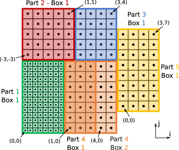
Figure 1: A semi-structured grid composed of five parts. Part 4 (orange) consists of two boxes, while the others consist of just a single box. Furthermore, Part 1 (green) has a refinement factor of two with respect to the other parts. The pairs $(x,y)$ denote cell coordinates in the $i$ and $j$ topological directions, respectively. Note that the indices of lower-left cells for each part are independent, since the grid parts live in different index spaces.

Stencils are used to define connections between neighboring grid cells of the same part, e.g., a typical five-point stencil would connect a generic grid cell to itself and its immediate neighbors to the west, east, south, and north. The graph describes how individual parts are connected, see Figure 3 for an example. We have now the components to define a semi-structured matrix $A=S+U$, which consists of structured and unstructured components, respectively. $S$ contains coefficients that are associated with stencil entries. These can be variable coefficients for each stencil entry in each cell within a part or can be set to just a single value if the stencil entry is constant across the part. $U$ is stored in ParCSR format and contains the connections between parts. Lastly, a semi-structured vector describes an array of values associated with the cells of a semi-structured grid.

3 Semi-structured algebraic multigrid (SSAMG)

In the hypre package, there is currently a single native preconditioner for solving problems with multiple parts through the SStruct interface, which is a block Jacobi method named Split. It uses one V-cycle of a structured multigrid solver as an approximation to the inverse of the structured part of $A$. This method has limited robustness since it considers only structured intra-grid couplings in a part to build an approximation of $A^{-1}$. In this paper, we present a new solver option for the SStruct interface that computes a multigrid hierarchy taking into account inter-part couplings. This method is called SSAMG (Semi-Structured Algebraic MultiGrid). It is currently available in the recmat branch of hypre. This section defines coarsening, interpolation, and relaxation for SSAMG (subsections 3.1, 3.2, and 3.4, respectively). It also describes how coarse level operators are constructed (subsection 3.3) and discusses a strategy for improving the method’s efficiency at coarse levels (subsection 3.5).

3.1 Coarsening

As in PFMG [2], we employ semi-coarsening in SSAMG. The coarsening directions are determined independently for each part of the SStructGrid to allow better treatment of problems with different anisotropies among the parts. The idea of semi-coarsening is to coarsen in a single direction of strong coupling such that every other perpendicular line/plane (2D/3D) forms the new coarse level. For an illustration, see Figure 3, where coarse points are depicted as solid circles.

In the original PFMG algorithm, the coarsening direction was chosen to be the dimension with smallest grid spacing. This option is still available in hypre by allowing users to provide an initial $n_{d}$-dimensional array of “representative grid spacings” that are only used for coarsening. However, both PFMG and SSAMG can also compute such an array directly from the matrix coefficients. In SSAMG, this is done separately for each part, leading to a matrix $W\in\mathbb{R}^{n_{p}\times n_{d}}$, where $n_{p}$ and $n_{d}$ denote the number of parts and problem dimensions. Here, element $W_{pd}$ is heuristically thought of as a grid spacing for dimension $d$ of part $p$, and hence a small value indicates strong coupling.

To describe the computation of $W$ in part $p$, consider the two-dimensional nine-point stencil in Figure 2c and assume that $A_{C}>0$ (simple sign adjustments can be made if $A_{C}<0$). The algorithm extends naturally to three dimensions. Note also that both PFMG and SSAMG are currently restricted to stencils that are contained within this nine-point stencil (27-point in 3D). The algorithm proceeds by first reducing the nine-point matrix to a single five-point stencil through an averaging process, then computing the (negative) sum of the resulting off-diagonal coefficients in each dimension. That is, for the $i$-direction ($d=1$), we compute

(2) $$c_{1}=\sum_{(i,j)}-(A_{SW}+A_{W}+A_{NW})-(A_{SE}+A_{E}+A_{NE}),$$

where the stencil coefficients are understood to vary at each point $(i,j)$ in the grid. Here the left and right parenthetical sums contribute to the “west” and “east” coefficients of the five-point stencil. The computation is analogous for the $j$-direction. From this, we define

(3) $$W_{pd}=\sqrt{\dfrac{\max\limits_{\begin{subarray}{c}0\leq i<n_{d}\end{subarray}}c_{i}}{c_{d}}},$$

based on the heuristic that the five-point stencil coefficients are inversely proportional to the square of the grid spacing.

With $W$ in hand, the semi-coarsening directions for each level and part are computed as described in Algorithm 1. The algorithm starts by computing a bounding box around the grid in each part, then loops through the grid levels from finest (level $0$) to coarsest (level $n_{l}$). For a given grid level $l$ and part $p$, the coarsening direction $d^{\star}$ is set to be the one with minimum value in $W_{p}$ (line 8). Then, the bounding box for part $p$ is coarsened by a factor of two in direction $d^{\star}$ (line 9) and $W_{p,d^{\star}}$ is updated to reflect the coarser “grid spacing” on the next grid level (line 10). If the bounding box is too small, no coarsening is done (line 7) and that part becomes inactive. The coarsest grid level $n_{l}$ is the first level with total semi-structured grid size less than a given maximum size $s_{max}$, unless this exceeds the specified maximum number of levels $l_{max}$.

Algorithm 1 SSAMG coarsening

1:procedure SSAMGCoarsen($W$)

2:     for $p=1,n_{p}$ do

3:         Compute part bounding boxes $bbox_{p}$

4:     end for

5:     for $l=1,n_{l}$ do

6:         for $p=1,n_{p}$ do

7:              if $\operatorname*{volume}{bbox_{p}}>1$ then

8:                  $d^{\star}=\operatorname*{arg\,min_{d}}{W_{pd}}$

9:                  Coarsen $bbox_{p}$ in direction $d^{\star}$ by a factor of 2

10:                  $W_{pd^{\star}}=2*W_{pd^{\star}}$

11:              end if

12:         end for

13:     end for

14:end procedure

3.2 Interpolation

A key ingredient in multigrid methods is the interpolation (or prolongation) operator $P$, the matrix that transfers information from a coarse level in the grid hierarchy to the next finer grid. The restriction operator $R$ moves information from a given level to the next coarser grid. For a numerically scalable method, error modes that are not efficiently reduced by relaxation should be captured in the range of $P$, so they can be reduced on coarser levels [7].

In SSAMG, we employ a structured operator-based method for constructing prolongation similar to the method used in [2]. It is “structured” because $P$ is composed of only a structured component; interpolation is only done within a part, not between them. It is “operator-based” because the coefficients are algebraically computed from $S$ and are able to capture heterogeneity and anisotropy. In hypre, $P$ is a rectangular matrix defined by two grids (domain and range), a stencil, and corresponding stencil coefficients. In the case of $P$, the domain grid is the coarse grid and the range grid is the fine grid. Since SSAMG uses semi-coarsening, the stencil for interpolation consists of three coefficients that are computed by collapsing the stencil of $A$, a common procedure for defining interpolation in algebraic multigrid methods.

To exemplify how $P$ is computed, consider the solution of the Poisson equation on a cell-centered grid (Figure 2a) formed by a single part and box. Dirichlet boundary conditions are used and discretization is performed via the finite difference method with a nine-point stencil (Figure 2c).

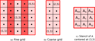
Figure 2: (a) and (b) show one example of fine and coarse grids, respectively, also known as range and domain grids for the purpose of prolongation. Coarsening is done in the $i$-direction, as depicted by the darker cells in the fine grid. (c) shows the stencil coefficients of $A$ relative to the grid point $(3,3)$ from the fine grid. Stencil coefficients for a given grid point can be viewed as the nonzero coefficients of its respective row in a sparse matrix.

Assume that coarsening is in the $i$-direction by selecting fine grid cells with even $i$-coordinate index (depicted in darker red) and renumbering them on the coarse grid as shown in Figure 2b. The prolongation operator connects fine grid cells to their neighboring coarse grid cells with the following stencil (see [11] for more discussion of stencil notation)

$$P\sim\big{[}P_{W}\quad 1\quad P_{E}\big{]}_{c}=\begin{bmatrix}P_{W}&*&P_{E}\end{bmatrix}^{r_{1}}_{c}\leavevmode\nobreak\ \oplus\leavevmode\nobreak\ \begin{bmatrix}*&1&*\end{bmatrix}^{r_{2}}_{c},$$

where

(4) $$P_{W}=\dfrac{A_{SW}+A_{W}+A_{NW}}{A_{S}+A_{C}+A_{N}},\;\text{and}\quad P_{E}=\dfrac{A_{SE}+A_{E}+A_{NE}}{A_{S}+A_{C}+A_{N}}.$$

Here, $r_{1}$ denotes the range subgrid given by the light-colored cells in Figure 2a, and $r_{2}$ denotes the subgrid given by the dark-colored cells. For a fine-grid cell such as $(3,3)$ in Figure 2, interpolation applies the weights $P_{W}$ and $P_{E}$ to the coarse-grid unknowns associated with cells $(2,3)$ and $(4,3)$ in the fine-grid indexing, or $(1,3)$ and $(2,3)$ in the coarse-grid indexing. For a fine-grid cell such as $(2,3)$, interpolation applies weight 1 to the corresponding coarse-grid unknown.

When one of the stencil entries crosses a part boundary that is not a physical boundary, we set the coefficient associated with it to zero and update the coefficient for the opposite stencil entry so that the vector of ones is contained in the range of the prolongation operator. Although this gives a lower order interpolation along part boundaries, it limits stencil growth and makes the computation of coarse level matrices cheaper, see section 3.3. It also assures that the near kernel of $A$ is well interpolated between subsequent levels.

Another component needed in a multigrid method is the restriction operator, which maps information from fine to coarse levels. SSAMG follows the Galerkin approach, where restriction is defined as the transpose of prolongation $(R=P^{T})$.

3.3 Coarse level operator

The coarse level operator $A_{c}$ in SSAMG is computed via the Galerkin product $P^{T}AP$. Since the prolongation matrix consists only of the structured component, the triple-matrix product can be rewritten as

(5) $$A_{c}=P^{T}SP+P^{T}UP,$$

where the first term on the right-hand side is the structured component of $A_{c}$, and the second its unstructured component. Note that the last term involves the multiplication of matrices of different types, which we resolve by converting one matrix type to the other. Since it is generally not possible to represent a ParCSR matrix in structured format, we convert the structured matrix $P$ to the ParCSR format. However, we consider only the entries of $P$ that are actually involved in the triple-matrix multiplication $P^{T}UP$ to decrease the computational cost of the conversion process.

If we examine the new stencil size for $A_{c}$, we note that the use of the two-point interpolation operator limits stencil growth. For example, in the case of a 2D five-point stencil at the finest level, the maximum stencil size on coarse levels is nine, and for a 3D seven-point stencil at the finest level, the maximum stencil size on coarse levels is 27.

We prove here that under certain conditions, the unstructured portion of the coarse grid operator stays restricted to the part boundaries and does not grow into the interior of the parts. Note that we define a part boundary $\delta\Omega_{i}$ here as the set of points in a part $\Omega_{i}$ that are connected to neighboring parts in the graph of the matrix $U$. For an illustration, see the black-rimmed points in Figure 3. Figure 3 shows the graph of $P$ for the semi-structured grid in Figure 1 and an example of a graph for the unstructured matrix $U$.

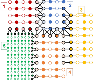
Figure 3: Example of a graph of the matrix $U$ and graph of matrix $P$ derived from the semi-structured grid shown in Figure 1. The graph of $U$ is depicted by black-solid edges. The graph of $P$ consists of five unconnected subgraphs illustrated by the dotted multicolored lines. Lastly, the boundary points are depicted by black-rimmed circles.

Theorem 3.1.

We make the following assumptions:

• The grid $\Omega$ consists of $k$ parts: $\Omega=\Omega_{1}\cup...\cup\Omega_{k}$, where $\Omega_{i}\cap\Omega_{j}=\emptyset$.

• The grid has been coarsened using semi-coarsening.

• The interpolation $P$ interpolates fine points using at most two adjacent coarse points aligned with the fine points and maps coarse points onto themselves.

• The graph of the unstructured matrix $U$ contains only connections between boundary points, i.e., $u_{i,j}=0$ if $i\in\Omega_{m}\setminus\delta\Omega_{m},m=1,...,k$, or $j\in\Omega_{n}\setminus\delta\Omega_{n},n=1,...,k$, and there are no connections within a part, i.e., $u_{i,j}=0$ for $i,j\in\Omega_{m},m=1,...,k.$

Then the graph of the unstructured part $U_{c}=P^{T}UP$ also contains only connections between boundary points, i.e., $u^{c}_{i,j}=0$ if $i\in\Omega^{c}_{m}\setminus\delta\Omega^{c}_{m},m=1,...,k$, or $j\in\Omega^{c}_{n}\setminus\delta\Omega^{c}_{n},n=1,...,k$, and there are no connections within a part, i.e., $u^{c}_{i,j}=0$ for $i,j\in\Omega^{c}_{m},m=1,...,k.$.

Proof 3.2.

Since we want to examine how boundary parts are handled, we reorder the interpolation matrix $P$ and the unstructured part $U$, so that all interior points are first followed by all boundary points. The matrices $P$ and $U$ are then defined as follows:

(6) $$P=\left(\begin{array}[]{cc}P^{I}&P^{IB}\\ P^{BI}&P^{B}\\ \end{array}\right),\leavevmode\nobreak\ \leavevmode\nobreak\ \leavevmode\nobreak\ \leavevmode\nobreak\ U=\left(\begin{array}[]{cc}0&0\\ 0&U^{B}\\ \end{array}\right).$$

Note that while $U^{B}$ maps $\delta\Omega$ onto $\delta\Omega$, $P^{B}$ maps $\delta\Omega_{c}$ onto $\delta\Omega$. Thus, in the extreme case that all boundary points are fine points, $P^{IB}$ and $P^{B}$ do not exist. Then, the coarse unstructured part is given as follows:

(7) $$U_{c}=P^{T}UP=\left(\begin{array}[]{cc}(P^{BI})^{T}U^{B}P^{BI}&(P^{BI})^{T}U^{B}P^{B}\\ (P^{B})^{T}U^{B}P^{BI}&(P^{B})^{T}U^{B}P^{B}\\ \end{array}\right).$$

It is clear already that there is no longer a connection to $P^{I}$ and $P^{IB}$, eliminating many potential connections to interior points; however, we still need to investigate further the influence of $P^{BI}$ and $P^{B}$.

Since $P^{BI}$, $P^{B}$, and $U^{B}$ are still very complex due to their dependence on $k$ parts, we further define them as follows using the fact that $P$ is defined only on the structured parts and $U$ only connects boundary points of neighboring parts.

(8) $$P^{x}=\left(\begin{array}[]{cccc}P^{x}_{1}&&&\\ &P^{x}_{2}&&\\ &&\ddots&\\ &&&P^{x}_{k}\\ \end{array}\right),\leavevmode\nobreak\ \leavevmode\nobreak\ \leavevmode\nobreak\ \leavevmode\nobreak\ U^{B}=\left(\begin{array}[]{cccc}0&U^{B}_{1,2}&...&U^{B}_{1,k}\\ U^{B}_{2,1}&0&\ddots&\vdots\\ \vdots&\ddots&\ddots&U^{B}_{k-1,k}\\ U^{B}_{k,1}&...&U^{B}_{k,k-1}&0\\ \end{array}\right).$$

Note that while $U_{ij}^{B}$ maps $\delta\Omega_{i}$ to $\delta\Omega_{j}$, only the coefficients corresponding to edges in the graph of $U$ that connect points in $\delta\Omega_{i}$ to $\delta\Omega_{j}$ are nonzero, all other coefficients are zero. Then, $(P^{x})^{T}U^{B}P^{y}$, where “$x$” and “$y$” can stand for “$BI$” as well as “$B$”, is given by

(9) $$\left(\begin{array}[]{cccc}0&(P^{x}_{1})^{T}U^{B}_{1,2}P^{y}_{2}&...&(P^{x}_{1})^{T}U^{B}_{1,k}P^{y}_{k}\\ (P^{x}_{2})^{T}U^{B}_{2,1}P^{y}_{1}&0&\ddots&\vdots\\ \vdots&\ddots&\ddots&(P^{x}_{k-1})^{T}U^{B}_{k-1,k}P^{y}_{k}\\ (P^{x}_{k})^{T}U^{B}_{k,1}P^{y}_{1}&...&(P^{x}_{k})^{T}U^{B}_{k,k-1}P^{y}_{k-1}&0\\ \end{array}\right).$$

This allows us to just focus on the submatrices $(P^{x}_{i})^{T}U^{B}_{ij}P^{y}_{j}$. There are three potential scenarios that can occur at the boundary between two parts due to our use of semi-coarsening and a simple two-point interpolation (Figure 3):

• all boundary points are coarse points as shown at the right boundary of part 2 and the left boundary of part 3;

• all boundary points are fine points as at the right boundary of part 1 and 4;

• the boundary points are alternating coarse and fine points as illustrated at the right boundary of part 5.

Let us define $P_{i}^{x}|_{\delta\Omega_{ij}}$ as the matrix that consists of the rows of $P_{i}^{x}$ that correspond to all boundary points in $\delta\Omega_{i}$ that are connected to boundary points in $\delta\Omega_{j}$. If all points are coarse points, $P_{i}^{B}|_{\delta\Omega_{ij}}=I$ and $P_{i}^{BI}|_{\delta\Omega_{ij}}=0$, since there are no connections from the boundary to the interior for $P_{i}^{BI}|_{\delta\Omega_{ij}}$. If all points are fine points, $P_{i}^{B}|_{\delta\Omega_{ij}}$ does not exist, and $P_{i}^{BI}|_{\delta\Omega_{ij}}$ is a matrix with at most one nonzero element per row. Since coarse points in $\Omega_{i}$ adjacent to the fine boundary points in $\delta\Omega_{i}$ become boundary points of $\Omega_{i}^{c}$, e.g., see right boundary of part 1 or left and right boundaries of part 4, all nonzero elements in $P_{i}^{BI}|_{\delta\Omega_{ij}}$ are associated with a column belonging to $\delta\Omega_{i}$. In the case of alternating fine and coarse points, $P_{i}^{BI}|_{\delta\Omega_{ij}}=0$, since there are no connections from the boundary to the interior, and $P_{i}^{B}|_{\delta\Omega_{ij}}$ is a matrix with at most two nonzeros in the $j$-th and $k$-th columns, where $j$ and $k$ are elements of $\delta\Omega_{i}^{c}$. Recall that all columns in $U_{ij}$ belonging to points outside of $\delta\Omega_{j}$ and all rows belonging to points outside of $\delta\Omega_{i}$ are zero. Based on this and the previous observations it is clear that if all points are coarse or we are dealing with alternating fine and coarse points, the submatrices in 9 that involve $P_{i}^{BI}$ will be 0, since $P_{i}^{BI}|_{\delta\Omega_{ij}}=0$ and $P_{j}^{BI}|_{\delta\Omega_{ji}}=0$. Any additional nonzero coefficients in $P_{i}^{BI}$ or $P_{j}^{BI}$ due to boundary points next to other parts will be canceled out in the matrix product. It is also clear, since the columns of $P_{i}^{B}$ pertain only to points in $\delta\Omega_{i}^{c}$, that the graph of the product $(P_{i}^{B})^{T}U_{ij}P_{j}^{B}$ only contains connections of points of $\delta\Omega_{i}^{c}$ to points of $\delta\Omega_{j}^{c}$ and none to the interior or to itself.

Let us further investigate the case where all boundary points are fine points. We first consider $(P_{i}^{BI})^{T}U_{ij}P_{j}^{BI}$. Since we have already shown that $P_{i}^{BI}|_{\delta\Omega_{ij}}=0$ for boundaries with coarse or alternating points leading to zero triple products in 9, we can ignore these scenarios and assume that for both $P_{i}^{BI}$ and $P_{j}^{BI}$ the boundary points adjacent to each other are fine points. Each row of $P_{i}^{BI}|_{\delta\Omega_{ij}}$ has at most one nonzero element in the column corresponding to the interior coarse point connected to the fine boundary point. This interior point is also an element in $\delta\Omega_{i}^{c}$. Therefore the graph of the product $(P_{i}^{BI})^{T}U_{ij}P_{j}^{BI}$ only contains connections of points of $\delta\Omega_{i}^{c}$ to points of $\delta\Omega_{j}^{c}$ and none to the interior or to itself. Finally, this statement also holds for the triple products $(P_{i}^{B})^{T}U_{ij}P_{j}^{BI}$ and $(P_{i}^{BI})^{T}U_{ij}P_{j}^{B}$ using the same arguments as above.

Note that the number of nonzero coefficients in $U_{c}$ can still be larger than those in $U$, however the growth only occurs along part boundaries.

3.4 Relaxation

Relaxation, or smoothing, is an important element of multigrid whose task is to eliminate high frequency error components from the solution vector $\mathbf{x}$. The relaxation process at step $k>0$ can be described via the generic formula:

(10) $$\mathbf{x}_{k}=\mathbf{x}_{k-1}+\omega M^{-1}\left(\mathbf{b}-A\mathbf{x}_{k-1}\right),$$

where $M^{-1}$ is the smoother operator and $\omega$ is the relaxation weight. In SSAMG, we provide two pointwise relaxation schemes. The first one is weighted Jacobi, in which $M^{-1}=D^{-1}$, with $D$ being the diagonal of $A$. Moreover, $\omega$ varies for each multigrid level and semi-structured part as a function of the grid-spacing metric $W$:

(11) $$\omega_{p}=\dfrac{2}{3-\beta_{p}/\alpha_{p}},$$

where

(12) $$\alpha_{p}=\sum^{n_{d}}_{d=0}\dfrac{1}{W^{2}_{pd}}\quad\text{and}\quad\beta_{p}=\sum^{n_{d}}_{\mathclap{\begin{subarray}{c}d\,=\,0,\\ d\neq d^{\star}\end{subarray}}}\dfrac{1}{W^{2}_{pd}}.$$

The ratio $\beta_{p}/\alpha_{p}$ adjusts the relaxation weight to more closely approximate the optimal weight for isotropic problems in different dimensions. To see how this works, consider as an example a highly-anisotropic 3D problem that is nearly decoupled in the $k$-direction and isotropic in $i$ and $j$. Because of the severe anisotropy, the problem is effectively 2D, so the optimal relaxation weight is $4/5$. Since our coarsening algorithm will only coarsen in either directions $i$ or $j$, we get $\beta_{p}/\alpha_{p}=1/2$, and $\omega_{p}=4/5$ as desired.

The second relaxation method supported by SSAMG is L1-Jacobi. This method is similar to the previous one, in the sense that a diagonal matrix is used to construct the smoother operator; however, here, the $i$-th diagonal element of $M$ equals the L1-norm of the $i$-th row of $A$:

$$M_{ii}=\sum\limits^{N}_{j=0}\left|A_{ij}\right|.$$

This form leads to guaranteed convergence when $A$ is positive definite, i.e., the error propagation operator $E=I-M^{-1}A$ has a spectral radius smaller than one. We refer to [3] for more details. This option tends to give slower convergence than weighted Jacobi; however, a user-defined relaxation factor in the range $(1,{2}/{\lambda_{max}(M^{-1}A)})$ ($\lambda_{max}$ is the maximum eigenvalue) can be used to improve convergence.

To reduce the computational cost of a multigrid cycle within SSAMG, we also provide an option to turn off relaxation on certain multigrid levels in isotropic (or partially isotropic) scenarios. We call this option “skip”, and it has the action of mimicking full-coarsening. For a given part, SSAMG’s algorithm checks if the coarsening directions for levels “$l$” and “$l-n_{d}$” match $\left(d^{\star}_{l}=d^{\star}_{l-n_{d}}\right)$. If yes, then relaxation is turned off (skipped) at level $l$.

3.5 Hybrid approach

Since SSAMG uses semi-coarsening, the coarsening ratio between the number of variables on subsequent grids is 2. In classical algebraic multigrid, this value tends to be larger, especially when aggressive coarsening strategies are applied. This leads to the creation of more levels in the multigrid hierarchy of SSAMG when compared to BoomerAMG. Since the performance benefits of exploiting structure decreases on coarser grid levels, we provide an option to transition to an unstructured multigrid hierarchy at a certain level or coarse problem size chosen by the user. This is done by converting the matrix type from SStructMatrix to ParCSRMatrix at the transition level. The rest of the multigrid hierarchy is set up using BoomerAMG configured with the default options used in hypre. With a properly chosen transition level, this hybrid approach can improve performance. In the non-hybrid case, SSAMG employs one sweep of the same relaxation method used in previous levels.

4 Numerical results

In this section, we investigate convergence and performance of SSAMG when used as a preconditioner for the conjugate gradient method (PCG). We also compare it to three other multigrid schemes in hypre, namely PFMG, Split, and BoomerAMG. The first is the flagship multigrid method for structured problems in hypre based on semi-coarsening [2, 8], the second, a block-Jacobi method built on top of the SStruct interface [21], in which blocks are mapped to semi-structured parts, and the last scheme is hypre’s unstructured algebraic multigrid method [19]. Each of these preconditioners has multiple setup parameters that affect its performance. For the comparison made here, we select those leading to the best solution times on CPU architectures. In addition, we consider four variants of SSAMG in an incremental setting to demonstrate the effects of different setup options described in the paper. A complete list of the methods considered here is given below:

• PFMG: weighted Jacobi smoother and “skip” option turned on.

• Split: block-Jacobi method with one V-cycle of PFMG as the inner solver for parts.

• BoomerAMG: Forward/Backward L1-Gauss-Seidel relaxation [3]; coarsening via HMIS [10] with a strength threshold value of $0.25$; modularized option for computing the Galerkin product $RAP$; one level (first) of aggressive coarsening with multi-pass interpolation [28] and, in the following levels, matrix-based extended+i interpolation [23] truncated to a maximum of four nonzero coefficients per row.

• SSAMG-base: baseline configuration of SSAMG employing weighted L1-Jacobi smoother with relaxation factor equal to $3/2$.

• SSAMG-skip: above configuration plus the “skip” option.

• SSAMG-hybrid: above configuration plus the “hybrid” option for switching to BoomerAMG as the coarse solver at the $10^{\text{th}}$ level, which corresponds to three steps of full grid refinement in 3D, i.e., $512$ times reduction on the number of degrees of freedom (DOFs).

• SSAMG-opt: refers to the best SSAMG configuration and employs the same parameters as SSAMG-hybrid except for switching to BoomerAMG at the $7^{\text{th}}$ level. This results in six pure SSAMG coarsening levels and reduction factor of $64$ on the number of DOFs.

Every multigrid preconditioner listed above is applied to the residual vector via a single V(1,1)-cycle. The coarsest grid size is at most 8 in all cases where BoomerAMG is used, it equals the number of parts for SSAMG-base and SSAMG-skip, and one for PFMG. The number of levels in the various multigrid hierarchies changes for different problem sizes and solvers.

We consider four test cases featuring three-dimensional semi-structured grids, different part distributions, and anisotropy directions. Each semi-structured part is formed by a box containing $m\times m\times m$ cells. Similarly, in a distributed parallel setting, each semi-structured part is owned by $p\times p\times p$ unique MPI tasks, meaning that the global semi-structured grid is formed by replicating the local $m^{3}$-sized boxes belonging to each part by $p$ times in each topological direction. This leads to a total of $n_{p}p^{3}$ MPI tasks for $n_{p}$ parts. We are particularly interested in evaluating weak scalability of the proposed method for a few tasks up to a range of thousands of MPI tasks. Thus, we vary the value of $p$ from one to eight with increments of one.

For the results, we report the number of iterations needed for convergence, setup time of the preconditioner, and solve time of the iterative solver. All experiments were performed on Lassen, a cluster at LLNL equipped with two IBM POWER9 processors (totaling $44$ physical cores) per node. However, we note that up to $32$ cores per node were used in the numerical experiments to reduce the effect of limited memory bandwidth. Convergence of the iterative solver is achieved when the L2-norm of the residual vector is less than $10^{-6}||\mathbf{b}||_{2}$. The linear systems were formed via discretization of the Poisson equation through the finite difference method, and zero Dirichlet boundary conditions are used everywhere except for the $k=0$ boundary, which assumes a value of one. The initial solution guess passed to PCG is the vector of zeros. The discretization scheme we used leads to the following seven-point stencil:

(13) $$A\sim\begin{bmatrix}-\gamma\end{bmatrix}\begin{bmatrix}&-\beta&\\ -\alpha&2(\alpha+\beta+\gamma)&-\alpha\\ &-\beta&\end{bmatrix}\begin{bmatrix}-\gamma\end{bmatrix}$$

where $\alpha$, $\beta$, and $\gamma$ denote the coefficients in the $i$, $j$, and $k$ topological directions. For the isotropic problems, $\alpha=\beta=\gamma=1$, for the anisotropic cases we define their values in section 4.2.

4.1 Test case 1 - cubes side-by-side

The first test case is made of an isotropic and block-structured three-dimensional domain composed of four cubes, where each contains the same number of cells and refers to a different semi-structured part. Figure 4 shows a plane view of one particular case with cubes formed by four cells in each direction. Regarding the solver choices, since PFMG works only for single-part problems, we translated parts into different boxes in an equivalent structured grid. Note that such a transformation is only possible due to the simplicity of the current problem geometry and is unattainable in more general cases such as those described later in sections 4.3 and 4.4.

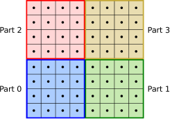
Figure 4: $ij$-plane cut of the three-dimensional base grid used for test case 4.1. There are no adjacent parts in the $k$-direction. Colors denote different parts, and the experiments showed in this section are produced by equally refining the base grid in all directions.

For the numerical experiments, we consider $m=128$, which gives a local problem size per part of $2,097,152$ DOFs and a global problem size of $8,388,608$ DOFs for 4 MPI tasks ($p=1$). The largest problem we consider here, obtained when $p=8$, has a global size of about $4.3$B DOFs.

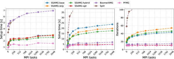
Figure 5: Weak scalability results for test case 1. Three metrics are shown in the figure, i.e., setup phase times in seconds (left); solve phase times in seconds (middle), and number of iterations (right). All curves are plotted with respect to the number of MPI tasks, $N_{\text{procs}}$, which varies from $4$ ($p=1$) up to $2048$ ($p=8$).

Figure 5 shows weak scalability results for this test case. Analyzing the iteration counts, Split is the only method that does not converge in less than a maximum iteration count of $100$ for runs larger than $500$M DOFs ($p=4$). This lack of numerical scalability was already expected since couplings among parts are not captured in Split’s multigrid hierarchy. The best iteration counts are reached by PFMG, which is natural since this method can take full advantage of the problem’s geometry. Noticeably, the iteration counts of SSAMG-opt follow PFMG closely, since part boundaries are no longer considered after switching to BoomerAMG on the coarser levels and the switch is done earlier here than in SSAMG-hybrid; the other SSAMG variants need a higher number of iterations for achieving convergence, since the interpolation is of lower quality along part boundaries. Lastly, the BoomerAMG preconditioner shows a modest increase in iteration counts for increasing problem sizes, and this is common in the context of algebraic multigrid.

Solve times are directly related to iteration counts. Since Split has a similar iteration cost to the other methods but takes the largest number of iterations to converge, it is the slowest option in solution time. For the same reason, the three SSAMG variants except for SSAMG-opt are slower than the remaining preconditioners. Still, SSAMG-skip is faster than SSAMG-base despite showing more iterations because the “skip”option reduces its iteration cost. The optimal variant SSAMG-opt is able to beat BoomerAMG by a factor of $1.6$x for $p=1$ and $2.3$x for $p=8$. Moreover, SSAMG-opt shows little performance degradation with respect to the fastest preconditioner (PFMG).

BoomerAMG is the slowest option when analyzing setup times. This is a result of multiple reasons, the three most significant ones being:

• BoomerAMG employs more elaborate formulas for computing interpolation, which require more computation time than the simple two-point scheme used by PFMG and SSAMG;

• the triple-matrix product algorithm for computing coarse operators implemented for CSR matrices is less efficient than the specialized algorithm employed by Struct and SStruct matrices;

• BoomerAMG’s coarsening algorithm involves choosing fine/coarse nodes on the matrix graph besides computing a strength of connection matrix. Those steps are not necessary for PFMG or SSAMG.

This is followed by Split, which should have setup times close to PFMG, but due to a limitation of its parallel implementation, the method does not scale well with an increasing number of parts. On the other hand, all the SSAMG variants show comparable setup times, up to $2.8$x faster than BoomerAMG. The first two SSAMG variants share the same setup algorithm, and their lines are superposed. SSAMG-opt has a slightly slower setup for $p\leq 5$ than SSAMG-base, but for $p>5$ the setup times of these two methods match. The fastest SSAMG variant by a factor of $1.2$x with respect to the others is SSAMG-hybrid, and that holds because it generates a multigrid hierarchy with fewer levels than the non-hybrid SSAMG variants leading to less communication overhead associated with collective MPI calls. The same argument is true for SSAMG-opt; however, the benefits of having fewer levels is outweighed by the cost of converting the SStructMatrix to a ParCSRMatrix in the switching level. Still, SSAMG-opt is $2.3$x and $3$x faster than BoomerAMG for $p=1$ and $p=8$, respectively. Finally, PFMG yields the best setup times with a speedup of nearly $4.6$x with respect to BoomerAMG and up to $1.9$x with respect to SSAMG.

We note that PFMG is naturally a better preconditioner for this problem than SSAMG since it interpolates across part boundaries. However, this test case was significant to show how close the performance of SSAMG can be to PFMG, and we demonstrated that SSAMG-opt is not much behind PFMG, besides yielding faster solve and setup times than BoomerAMG.

4.2 Test case 2 - anisotropic cubes

This test case has the same problem geometry and sizes ($m=128$) as the previous test case; however, it employs different stencil coefficients ($\alpha$, $\beta$, and $\gamma$) for each part of the grid with the aim of evaluating how anisotropy affects solver performance. Particularly, we consider three different scenarios (Figure 6) where the coefficients relative to stencil entries belonging to the direction of strongest anisotropy for a given part are $100$ times larger than the remaining ones. The directions of prevailing anisotropy for each scenario are listed below:

1. “$i$” (horizontal) for all semi-structured parts.

2. “$i$” for parts zero and two; “$j$” (vertical) for parts one and three.

3. “$i$” for part zero, “$j$” for part three, and “$k$” (depth) for parts one and two.

Regarding the usage of PFMG for this problem, the same transformation mentioned in section 4.1 apply here as well.

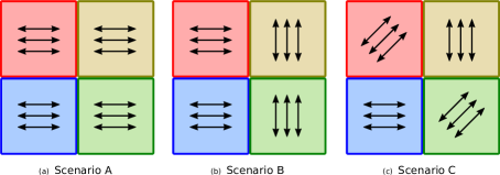
Figure 6: $XY$-plane cut of the three-dimensional grids used in test case 4.2. We consider three anisotropy scenarios. Arrows indicate the direction of prevailing anisotropy in each part of the grid, e.g., $i$-direction in scenario A. Diagonal arrows in the rightmost case indicate the $k$-direction.

Figure 7 shows the results referent to scenario A. The numerical scalabilities of the different methods look better than in the previous test case. This is valid especially for the SSAMG variants, because the two-point interpolation strategy is naturally a good choice for the first few coarsening levels when anisotropy is present in the matrix coefficients. Such observation also applies to the less scalable Split method, explaining the better behavior seen here with respect to Figure 5. Again, PFMG uses the least number of iterations followed closely by SSAMG-opt and BoomerAMG.

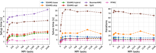
Figure 7: Weak scalability results for scenario A of test case 2. Three metrics are shown in the figure, i.e., setup phase times in seconds (left); solve phase times in seconds (middle), and number of iterations (right). All curves are plotted with respect to the number of MPI tasks, $N_{\text{procs}}$, which varies from $4$ ($p=1$) up to $2048$ ($p=8$).

Regarding solve times, SSAMG-opt is about $1.3$x faster than BoomerAMG for $p\leq 2$, while for $p>2$ these methods show similar times. The “skip” option of SSAMG is not beneficial for this case since the solve times of SSAMG-skip are higher than SSAMG-base. In fact, such an option does not play a significant role in reducing the solve time compared to isotropic test cases. This is because coarsening happens in the same direction for the first few levels in anisotropic test cases, and thus relaxation is skipped only in the later levels of the multigrid hierarchy where the cost per iteration associated with them is already low compared to the initial levels. Moreover, the omission of relaxation in coarser levels of the multigrid hierarchy can be detrimental for convergence in SSAMG, explaining why SSAMG-skip requires more iterations than SSAMG-base. Following the fact that PFMG is the method that needs fewer iterations for convergence, it is also the fastest in terms of solution times. For setup times, the four SSAMG variants show comparable results, and similar conclusions to test case 1 are valid here. Lastly, the speedups of SSAMG-opt over BoomerAMG are $3.3$x and $2.5$x for $p=1$ and $p=8$, respectively.

Results for scenario B are shown in Figure 8. The most significant difference here compared to scenario A are the results for PFMG. Particularly, the number of iterations is much higher than in the previous cases. This is caused by the fact that PFMG employs the same coarsening direction everywhere on the grid, and thus it cannot recognize the different regions of anisotropy as done by SSAMG. This is clearly sub-optimal since a good coarsening scheme should adapt to the direction of largest coupling of the matrix coefficients. The larger number of iterations is also reflected in the solve times of PFMG, which become less favorable than those by SSAMG and BoomerAMG. Setup times of PFMG continue to be the fastest ones; however, this advantage is not sufficient to maintain its position of fastest method overall. The comments regarding the speedups of SSAMG compared to BoomerAMG made for scenario A also apply here.

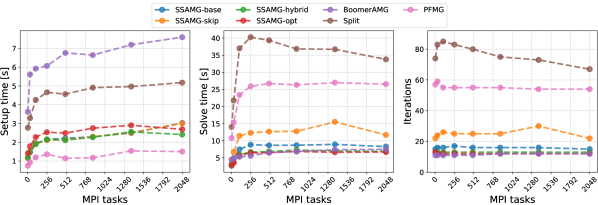
Figure 8: Weak scalability results for scenario B of test case 2. Three metrics are shown in the figure, i.e., setup phase times in seconds (left); solve phase times in seconds (middle), and number of iterations (right). All curves are plotted with respect to the number of MPI tasks, $N_{\text{procs}}$, which varies from $4$ ($p=1$) up to $2048$ ($p=8$).

We conclude this section by analyzing the results, given in Figure 9, for the last anisotropy scenario C. Since there is a mixed anisotropy configuration in this case as in scenario B, PFMG does not show a satisfactory convergence behavior. On the other hand, the SSAMG variants show good numerical and computational scalabilities, and, particularly, SSAMG-opt shows similar speedups compared to the BoomerAMG variants as discussed in the previous scenarios. When considering all three scenarios discussed in this section, we note that SSAMG shows good robustness with changes in anisotropy, and this an important advantage over PFMG.

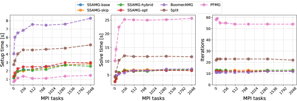
Figure 9: Weak scalability results for scenario C of test case 2. Three metrics are shown in the figure, i.e., setup phase times in seconds (left); solve phase times in seconds (middle), and number of iterations (right). All curves are plotted with respect to the number of MPI tasks, $N_{\text{procs}}$, which varies from $4$ ($p=1$) up to $2048$ ($p=8$).

4.3 Test case 3 - three-points intersection

In this test case, we consider a grid composed topologically of three semi-structured cubic parts that share a common intersection edge in the $k$-direction (Figure 10). Stencil coefficients are isotropic, but this test case is globally non-Cartesian. In particular, the coordinate system is different on either side of the boundary between parts 1 and 2. For example, an east stencil coefficient coupling Part 1 to Part 2 is symmetric to a north coefficient coupling Part 2 to Part 1.

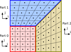
Figure 10: $ij$-plane view of the base geometry for test case 4.3. Equally refined instances of this problem in all directions are used for obtaining the results.

For the numerical experiments of this section, we use $m=160$, which gives a local problem size per part of $4,096,000$ DOFs, and a global problem size of $12,288,000$ DOFs, when $p=1$, i.e., three parts and MPI tasks. Figure 11 reports weak scalability results for the current test case. As noted in section 4.1, it is not possible to recast this problem into a single part; thus, we cannot show results for PFMG here.

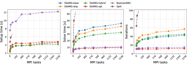
Figure 11: Weak scalability results for test case 3. Three metrics are shown in the figure, i.e., setup phase times in seconds (left); solve phase times in seconds (middle), and number of iterations (right). All curves are plotted with respect to the number of MPI tasks, $N_{\text{procs}}$, which varies from $3$ ($p=1$) up to $1536$ ($p=8$).

Examining the iteration counts reported in Figure 11, we see that SSAMG-opt is the fastest converging option with the number of iterations ranging from $11$, for $p=1$ ($3$ MPI tasks), to $14$, for $p=8$ ($1536$ MPI tasks). This is the best numerical scalability among the other methods, including BoomerAMG. On the other hand, the remaining SSAMG variants do not show such good scalability as in the previous test cases. Once again, this is related to how SSAMG computes interpolation weights of nodes close to part boundaries. In this context, we plan to investigate further how to improve SSAMG’s interpolation such that the non-hybrid SSAMG variants can have similar numerical scalability to SSAMG-opt. As in the previous test cases, the Split method is the least performing method and does not converge within 100 iterations for $p\geq 3$ ($N_{p}\geq 81$).

Regarding solve times, SSAMG-opt is the fastest method since it needs the minimum amount of iterations to reach convergence. Compared to BoomerAMG, its speedup is $1.3$x for $p=1$ and $1.1$x for $p=8$. SSAMG-skip shows solution times smaller than SSAMG-base, and, here, the “skip” option is beneficial to performance. Lastly, looking at setup times, all SSAMG variants show very similar timings and the optimal variant is up to $2.9$x faster than BoomerAMG, proving once again the benefits of exploiting problem structure.

4.4 Test case 4 - structured adaptive mesh refinement (SAMR)

In the last problem, we consider a three-dimensional SAMR grid consisting of one level of grid refinement, and thus composed of two semi-structured parts (Figure 12). The first one, in red, refers to the outer coarse grid, while the second, in blue, refers to the refined patch (by a factor of two) located in the center of the grid. Each part has the same number of cells. To construct the linear system matrix for this problem, we treat coarse grid points living inside of the refined part as ghost unknowns, i.e., the diagonal stencil entry for these points is set to one and the remaining off-diagonal stencil entries are set to zero. Inter-part couplings at fine-coarse interfaces are stored in the unstructured matrix ($U$), and the value for the coefficients connecting fine grid cells with its neighboring coarse grid cells (and vice-versa) is set to $2/3$. This value was determined by composing a piecewise constant interpolation formula with a finite volume discretization rule. We refer the reader to the SAMR section of hypre’s documentation [21] for more details.

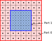
Figure 12: $XY$-plane cut of the three-dimensional semi-structured grid used in test case 4.4 when $m=8$. The semi-structured parts represent two levels of refinement and contain the same number of cells.

The numerical experiments performed in this section used $m=128$, leading to a local problem size per part of $2,097,152$ DOFs, and a global problem size of $4,194,304$ DOFs, for $p=1$ ($N_{\text{procs}}=2$). Figure 13 shows weak scalability results for this test case. This problem is not suitable for PFMG, thus we do not show results for PFMG.

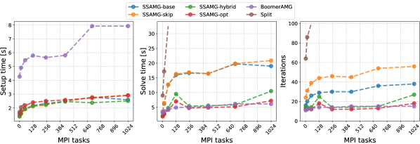
Figure 13: Weak scalability results for test case 4. Three metrics are shown in the figure, i.e., setup phase times in seconds (left); solve phase times in seconds (middle), and number of iterations (right). All curves are plotted with respect to the number of MPI tasks, $N_{\text{procs}}$, which varies from $2$ ($p=1$) up to $1024$ ($p=8$).

As in the previous test cases, Split does not reach convergence within 100 iterations when $p\geq 3$. Then, SSAMG-skip is the second least convergent option followed by SSAMG-base. The best option is again SSAMG-opt with the number of iterations ranging from $15$ ($p=1$) to $20$ ($p=8$). Furthermore, its iteration counts are practically constant for the several parallel runs, except for slight jumps located at $p=4$ ($N_{\text{procs}}=128$) and $p=8$ ($N_{\text{procs}}=1024$), which are present in SSAMG-hybrid as well.

As noted before, solve times reflect the methods’ convergence performance. In particular, the cheaper iterations of SSAMG-skip are not able to offset the higher number of iterations for convergence over SSAMG-base. That explains why these two methods show very similar solve times. Split is the least performing option due to its lack of robustness. SSAMG-opt and BoomerAMG have similar performance, with SSAMG-opt slightly better for various cases, but BoomerAMG showing more consistent performance here.

Setup times of the SSAMG variants are very similar. Listing them in decreasing order of times, SSAMG-base and SSAMG-skip show nearly the same values, followed by SSAMG-opt, and SSAMG-hybrid is the fastest option. The results for Split are better here than in the previous test cases, and this is due to the small number of semi-structured parts involved in this SAMR problem. Still, SSAMG leads to the fastest options. The slowest method for setup is again BoomerAMG and SSAMG-opt speedups with respect to it are $4$x for $p=1$ and $2.7$x for $p=8$.

5 Conclusions

In this paper, we presented a novel algebraic multigrid method, built on the semi-structured interface in hypre, capable of exploiting knowledge about the problem’s structure and having the potential of being faster than an unstructured algebraic multigrid method such as BoomerAMG on CPUs and accelerators. Moreover, SSAMG features a multigrid hierarchy with controlled stencil sizes and significantly improved setup times.

We developed a distributed parallel implementation of SSAMG for CPU architectures in hypre. Furthermore, we tested its performance, when used as a preconditioner to PCG, for a set of semi-structured problems featuring distinct characteristics in terms of grid, stencil coefficients, and anisotropy. SSAMG proves to be numerically scalable for problems having up to a few billion degrees of freedom and its current implementation achieves setup phase speedups up to a factor of four and solve phase speedups up to $1.4$x with respect to BoomerAMG.

For future work, we plan to improve different aspects of SSAMG and its implementation. We will further investigate SSAMG convergence for more complex problems than have been considered so far. We want to explore adding an unstructured component to the prolongation matrix to improve interpolation across part boundaries and evaluate how this benefits convergence and time to solution. We also plan to add a non-Galerkin option for computing coarse operators targeting isotropic problems since this approach applied in PFMG has shown excellent runtime improvements on both CPU and GPU. Finally, we will develop a GPU implementation for SSAMG.

References

- [1] S. Adams, R. Ford, M. Hambley, J. Hobson, I. Kavčič, C. Maynard, T. Melvin, E. Müller, S. Mullerworth, A. Porter, M. Rezny, B. Shipway, and R. Wong, LFRic: Meeting the challenges of scalability and performance portability in weather and climate models, Journal of Parallel and Distributed Computing, 132 (2019), pp. 383–396, https://doi.org/10.1016/j.jpdc.2019.02.007.
- [2] S. F. Ashby and R. D. Falgout, A parallel multigrid preconditioned conjugate gradient algorithm for groundwater flow simulations, Nuclear Science and Engineering, 124 (1996), pp. 145 – 159, https://doi.org/10.13182/nse96-a24230.
- [3] A. H. Baker, R. D. Falgout, T. V. Kolev, and U. M. Yang, Multigrid smoothers for ultraparallel computing, SIAM Journal on Scientific Computing, 33 (2011), pp. 2864–2887, https://doi.org/10.1137/100798806.
- [4] A. H. Baker, R. D. Falgout, T. V. Kolev, and U. M. Yang, Scaling Hypre’s Multigrid Solvers to 100,000 Cores, Springer London, London, 2012, pp. 261–279, https://doi.org/10.1007/978-1-4471-2437-5_13.
- [5] B. Bergen, G. Wellein, F. Hülsemann, and U. Rüde, Hierarchical hybrid grids: achieving TERAFLOP performance on large scale finite element simulations, International Journal of Parallel, Emergent and Distributed Systems, 22 (2007), pp. 311–329, https://doi.org/10.1080/17445760701442218.
- [6] B. K. Bergen and F. Hülsemann, Hierarchical hybrid grids: data structures and core algorithms for multigrid, Numerical Linear Algebra with Applications, 11 (2004), pp. 279–291, https://doi.org/10.1002/nla.382.
- [7] W. L. Briggs, V. E. Henson, and S. F. McCormick, A Multigrid Tutorial, Second Edition, Society for Industrial and Applied Mathematics, second ed., 2000, https://doi.org/10.1137/1.9780898719505.
- [8] P. N. Brown, R. D. Falgout, and J. E. Jones, Semicoarsening multigrid on distributed memory machines, SIAM Journal on Scientific Computing, 21 (2000), pp. 1823–1834, https://doi.org/10.1137/S1064827598339141.
- [9] S. L. Cornford, D. F. Martin, D. T. Graves, D. F. Ranken, A. M. Le Brocq, R. M. Gladstone, A. J. Payne, E. G. Ng, and W. H. Lipscomb, Adaptive mesh, finite volume modeling of marine ice sheets, Journal of Computational Physics, 232 (2013), pp. 529–549, https://doi.org/10.1016/j.jcp.2012.08.037.
- [10] H. De Sterck, U. M. Yang, and J. J. Heys, Reducing complexity in parallel algebraic multigrid preconditioners, SIAM Journal on Matrix Analysis and Applications, 27 (2006), pp. 1019–1039, https://doi.org/10.1137/040615729.
- [11] C. Engwer, R. D. Falgout, and U. M. Yang, Stencil computations for PDE-based applications with examples from DUNE and hypre, Concurrency and Computation: Practice and Experience, 29 (2017), p. e4097, https://doi.org/10.1002/cpe.4097.
- [12] R. D. Falgout, J. E. Jones, and U. M. Yang, Conceptual interfaces in hypre, Future Generation Computer Systems, 22 (2006), pp. 239–251, https://doi.org/10.1016/j.future.2003.09.006.
- [13] R. D. Falgout, J. E. Jones, and U. M. Yang, The design and implementation of hypre, a library of parallel high performance preconditioners, in Numerical Solution of Partial Differential Equations on Parallel Computers, A. M. Bruaset and A. Tveito, eds., Berlin, Heidelberg, 2006, Springer Berlin Heidelberg, pp. 267–294, https://doi.org/10.1007/3-540-31619-1_8.
- [14] R. D. Falgout, R. Li, B. Sjögreen, L. Wang, and U. M. Yang, Porting hypre to heterogeneous computer architectures: Strategies and experiences, Parallel Computing, 108 (2021), p. 102840, https://doi.org/10.1016/j.parco.2021.102840.
- [15] R. D. Falgout and U. M. Yang, hypre: A library of high performance preconditioners, in Computational Science — ICCS 2002, P. M. A. Sloot, A. G. Hoekstra, C. J. K. Tan, and J. J. Dongarra, eds., Berlin, Heidelberg, 2002, Springer Berlin Heidelberg, pp. 632–641, https://doi.org/10.1007/3-540-47789-6_66.
- [16] B. Ganis, G. Pencheva, and M. F. Wheeler, Adaptive mesh refinement with an enhanced velocity mixed finite element method on semi-structured grids using a fully coupled solver, Computational Geosciences, 23 (2019), pp. 1573–1499, https://doi.org/10.1007/s10596-018-9789-6.
- [17] B. Gmeiner and U. Rüde, Peta-scale hierarchical hybrid multigrid using hybrid parallelization, in Large-Scale Scientific Computing, I. Lirkov, S. Margenov, and J. Waśniewski, eds., Berlin, Heidelberg, 2014, Springer Berlin Heidelberg, pp. 439–447, https://doi.org/10.1007/978-3-662-43880-0_50.
- [18] B. Gmeiner, U. Rüde, H. Stengel, C. Waluga, and B. Wohlmuth, Towards textbook efficiency for parallel multigrid, Numerical Mathematics: Theory, Methods and Applications, 8 (2015), p. 22–46, https://doi.org/10.4208/nmtma.2015.w10si.
- [19] V. E. Henson and U. M. Yang, BoomerAMG: A parallel algebraic multigrid solver and preconditioner, Applied Numerical Mathematics, 41 (2002), pp. 155–177, https://doi.org/10.1016/S0168-9274(01)00115-5. Developments and Trends in Iterative Methods for Large Systems of Equations - in memorium Rudiger Weiss.
- [20] R. D. Hornung and S. R. Kohn, Managing application complexity in the SAMRAI object-oriented framework, Concurrency and Computation: Practice and Experience, 14 (2002), pp. 347–368, https://doi.org/10.1002/cpe.652.
- [21] hypre: High performance preconditioners. http://www.llnl.gov/CASC/hypre/, https://github.com/hypre-space/hypre.
- [22] N. Kohl and U. Rüde, Textbook efficiency: massively parallel matrix-free multigrid for the stokes system, (2020), https://doi.org/10.48550/arXiv.2010.13513.
- [23] R. Li, B. Sjögreen, and U. M. Yang, A new class of AMG interpolation methods based on matrix-matrix multiplications, SIAM Journal on Scientific Computing, 43 (2021), pp. S540–S564, https://doi.org/10.1137/20M134931X.
- [24] M. Mayr, L. Berger-Vergiat, P. Ohm, and R. S. Tuminaro, Non-invasive multigrid for semi-structured grids, 2021, https://doi.org/10.48550/arXiv.2103.11962.
- [25] C. Rodrigo, F. J. Gaspar, and F. J. Lisbona, Multigrid methods on semi-structured grids, Archives of Computational Methods in Engineering, 19 (2012), pp. 499–538, https://doi.org/10.1007/s11831-012-9078-9.
- [26] B. Runnels, V. Agrawal, W. Zhang, and A. Almgren, Massively parallel finite difference elasticity using block-structured adaptive mesh refinement with a geometric multigrid solver, Journal of Computational Physics, 427 (2021), p. 110065, https://doi.org/10.1016/j.jcp.2020.110065.
- [27] K. Stüben, A review of algebraic multigrid, Journal of Computational and Applied Mathematics, 128 (2001), pp. 281–309, https://doi.org/10.1016/S0377-0427(00)00516-1. Numerical Analysis 2000. Vol. VII: Partial Differential Equations.
- [28] U. M. Yang, On long-range interpolation operators for aggressive coarsening, Numerical Linear Algebra with Applications, 17 (2010), pp. 453–472, https://doi.org/10.1002/nla.689.
- [29] W. Zhang, A. Almgren, V. Beckner, J. Bell, J. Blaschke, C. Chan, M. Day, B. Friesen, K. Gott, D. Graves, et al., AMReX: a framework for block-structured adaptive mesh refinement, Journal of Open Source Software, 4 (2019), pp. 1370–1370, https://doi.org/10.21105/joss.01370.
- [30] W. Zhang, A. Myers, K. Gott, A. Almgren, and J. Bell, AMReX: Block-structured adaptive mesh refinement for multiphysics applications, The International Journal of High Performance Computing Applications, 35 (2021), pp. 508–526, https://doi.org/10.1177/10943420211022811.