Temporal graph patterns by timed automata

Abstract

Temporal graphs represent graph evolution over time, and have been receiving considerable research attention. Work on expressing temporal graph patterns or discovering temporal motifs typically assumes relatively simple temporal constraints, such as journeys or, more generally, existential constraints, possibly with finite delays. In this paper we propose to use timed automata to express temporal constraints, leading to a general and powerful notion of temporal basic graph pattern (BGP).

The new difficulty is the evaluation of the temporal constraint on a large set of matchings. An important benefit of timed automata is that they support an iterative state assignment, which can be useful for early detection of matches and pruning of non-matches. We introduce algorithms to retrieve all instances of a temporal BGP match in a graph, and present results of an extensive experimental evaluation, demonstrating interesting performance trade-offs. We show that an on-demand algorithm that processes total matchings incrementally over time is preferable when dealing with cyclic patterns on sparse graphs. On acyclic patterns or dense graphs, and when connectivity of partial matchings can be guaranteed, the best performance is achieved by maintaining partial matchings over time and allowing automaton evaluation to be fully incremental. The code and datasets are available at http://github.com/amirpouya/TABGP.

1 Introduction

Graph pattern matching, the problem of finding instances of one graph in a larger graph, has been extensively studied since the 1970s, and numerous algorithms have been proposed cheng2008fast ; conte2004thirty ; fan2010graph ; lai2019distributed ; reza2020approximate ; ullmann1976algorithm . Initially, work in this area focused on static graphs, in which information about changes in the graph is not recorded. Finding patterns in static graphs can be helpful for many important tasks, such as finding mutual interests among users in a social network. However, understanding how interests of social network users evolve over time, support for contact tracing, and many other research questions and applications require access to information about how a graph changes over time. Consequently, the focus of research has shifted to pattern matching in temporal graphs for tasks such as finding temporal motifs, temporal journeys, and temporal shortest paths DBLP:conf/sigmod/GurukarRR15 ; DBLP:journals/corr/abs-1107-5646 ; DBLP:conf/wsdm/ParanjapeBL17 ; rost2022distributed ; semertzidis2016durable ; xu2017time ; zfy-temporal-clique ; DBLP:conf/edbt/ZufleREF18 .

Figure 1: Example of a temporal graph. Each edge is associated with the set of timepoints during which it is active.

Figure 1 gives our running example, showing an interaction graph, where each node represents an employee (node label emp), a customer (cst), or an office (ofc), and each edge represents either an email message (msg) or a visit (visit) from a source node to a target node. Each edge is associated with the set of timepoints when an interaction occurred. Such graphs with static nodes but dynamic edges that are active at multiple timepoints are commonly used to represent interaction networks DBLP:conf/wsdm/ParanjapeBL17 ; zhao2010Comm .

Example 1

Assume our temporal graph holds information about a publicly traded company. Suppose that employee $v_{1}$ shared confidential information with their colleagues $v_{2}$ and $v_{3}$, and that one of them subsequently shared this information with customer $v_{4}$, potentially constituting insider trading. Assuming that we have no access to the content of the messages, only to when they were sent, can we identify employees who may have leaked confidential information to $v_{4}$?

Based on graph topology alone, both $v_{2}$ and $v_{3}$ could have been the source of the information leak to $v_{4}$. However, by considering the timepoints on the edges, we observe that there is no path from $v_{1}$ to $v_{4}$ that goes through $v_{3}$ and visits the nodes in temporal order. We will represent this scenario with the following basic graph pattern (BGP), augmented with a temporal constraint:

$$\mathsf{v_{1}}\xrightarrow{y_{1}}x\xrightarrow{y_{2}}\mathsf{v_{4}}:\exists t_{1}\in y_{1}.T,\,\exists t_{2}\in y_{2}.T:t_{1}\leqslant t_{2}$$

Here, $\mathsf{v_{1}}$ and $\mathsf{v_{4}}$ are node constants, $x$ is a node variable, $y_{1}$ and $y_{2}$ are edge variables, and $y_{1}.T$ and $y_{2}.T$ refer to the sets of timepoints associated with edges $y_{1}$ and $y_{2}$. The temporal constraint states that there must exist a pair of timepoints $t_{1}$, associated with edge $y_{1}$, and $t_{2}$, associated with edge $y_{2}$, such that $t_{1}$ occurs before $t_{2}$. We refer to such combinations of BGPs and temporal constraints as temporal BGPs.

The temporal constraint in the above example is existential: it requires the existence of timepoints where the edges from a BGP matchings are active, so that these timepoints satisfy some condition (in the example, a simple inequality). Existential constraints are typical in the literature on temporal graph pattern matching DBLP:conf/sigmod/GurukarRR15 ; DBLP:conf/wsdm/ParanjapeBL17 ; semertzidis2016durable ; xu2017time ; zfy-temporal-clique ; DBLP:conf/edbt/ZufleREF18 . Various forms of conditions, beyond inequalities on the timepoints, have been considered. For example, one may require that the timepoints belong to a common interval with a given start- and end-time (“temporal clique” zfy-temporal-clique ) or with a given length (“$\delta$-motifs” DBLP:conf/wsdm/ParanjapeBL17 ), or one may specify lower and upper bounds on the gaps between the timepoints DBLP:conf/edbt/ZufleREF18 .

In this paper, our goal is to go beyond existential constraints. Indeed, many useful temporal constraints are not existential. We give two examples over temporal graphs such as the one in Figure 1.

Example 2

When monitoring communication patterns, we may want to look for extended interactions between customers and employees. Specifically, we are looking for matchings of the BGP shown in Figure 2a, where edge variables $y_{1}$ and $y_{2}$ represent email messages exchanged by customer $x_{1}$ and employee $x_{2}$. We impose the temporal constraint that $y_{1}$ and $y_{2}$ are active in an interleaved, alternating fashion: first $y_{1}$ was active, then $y_{2}$, then $y_{1}$ again, etc. This constraint is not existential. In Figure 1, it is satisfied in the communication between $v_{5}$ and $v_{1}$, but not between $v_{7}$ and $v_{1}$.

Example 3

In contact tracing, we may want to look for pairs of employees who have shared an office for a contiguous period of time with some minimal duration. We are looking for matchings of the BGP $x_{2}:{\tt{emp}}\xrightarrow{y_{1}:{\tt{visit}}}x_{1}:{\tt{ofc}}\xleftarrow{y_{2}:{\tt{visit}}}x_{3}:{\tt{emp}}$. As a temporal constraint, we impose that there exists a contiguous sequence of timepoints in the graph’s temporal domain, of duration at least, say, 3 time units, in which $y_{1}$ and $y_{2}$ were both active. This constraint is, again, not existential. In Figure 1, the only matching of the BGP (involving employees $v_{2}$ and $v_{4}$ and office $v_{8}$) does not satisfy the constraint; as a matter of fact, $v_{2}$ and $v_{4}$ were never active (i.e., at the office) at the same time! Indeed, “$y_{1}$ and $y_{2}$ are never active at the same time” would be another natural example of a temporal constraint that is not existential.

In order to express temporal constraints (existential or not), we need a language. When the goal is the expression of possibly complex constraints, an obvious approach would be to use SQL. Indeed, any temporal graph can be naturally represented by three relations $\mathit{Node}(\mathit{vid},\mathit{label})$, $\mathit{Edge}(\mathit{eid},\mathit{vid}_{1},\mathit{vid}_{2},\mathit{label})$, and $\mathit{Active}(\mathit{eid},\mathit{time})$, where $\mathit{vid}$ and $\mathit{eid}$ are node (vertex) and edge identifiers. The problem with this approach is that temporal constraints do not fit well in the SQL idiom. SQL is certainly expressive enough, but the resulting expressions tend to be complicated and hard to optimize. The alternating communication pattern from Example 2 would be expressed in SQL as follows:

⬇

QTA1: WITH matching AS

(SELECT E1.eid AS y1, E2.eid AS y2

FROM edge E1, edge AS E2

WHERE E1.dst = E2.src and E2.dst = E1.src),

Succ AS

(SELECT y1, y2, A1.eid AS e1, A2.eid AS e2

FROM matching, active A1, active A2

WHERE (A1.eid = y1 OR A1.eid = y2)

AND (A2.eid = y1 OR A2.eid = y2)

AND A1.time<A2.time AND NOT EXISTS

(SELECT * FROM active A3

WHERE (A3.eid = y1 or A3.eid = y2)

AND A1.time<A3.time

AND A3.time<A2.time))

SELECT * FROM matching M

WHERE NOT ( EXISTS (SELECT * FROM active WHERE eid = y2)

AND NOT EXISTS (SELECT * FROM active WHERE eid = y1) )

AND ( NOT EXISTS (SELECT * FROM active A1, active A2

WHERE A1.eid = y1 AND A2.eid = y2)

OR (SELECT MIN(time) FROM active WHERE eid = y1) <

(SELECT MIN(time) FROM active WHERE eid = y2) )

AND NOT EXISTS (SELECT * FROM Succ

WHERE M.y1 = y1 AND M.y2 = y2 AND e1 = e2)

Likewise, for the contiguous-duration office sharing pattern from Example 3:

⬇

QTA7: WITH matching AS

(SELECT E1.eid AS y1, E2.eid AS y2

FROM edge E1, edge AS E2 WHERE E1.dst = E2.dst)

SELECT DISTINCT y1, y2

FROM matching, active A1, active A2, active B1, active B2

WHERE A1.eid = y1 AND A2.eid = y2 AND A1.time = A2.time

AND B1.eid = y1 AND B2.eid = y2 AND B1.time = B2.time

AND B1.time - A1.time > 3

AND NOT EXISTS

(SELECT * FROM active C

WHERE A1.time < C.time AND C.time < B1.time

AND NOT EXISTS (SELECT * FROM active C1, active C2

WHERE C1.time = C.time AND C2.time = C.time

AND C1.eid = y1 AND C2.eid = y2))

The hypothesis put forward in this paper is that specification formalisms used in fields such as complex event recognition stijn-cer or verification of real-time systems timed-automata-survey may be much more suitable for the expression of complex temporal constraints. In this paper, we specifically investigate the use of timed automata timed-automata ; timed-automata-survey .

Example 4

Figure 2 shows various examples of timed automata that can be applied to matchings of a BGP with two edge variables $y_{1}$ and $y_{2}$, such as the BGPs considered in Examples 2 and 3. One can think of the automaton as running over the snapshots of the temporal graph. A matching is accepted if there is a run such that, after seeing the last snapshot, the automaton is in an accepting state. The edge variables serve as Boolean conditions on the transitions of the automaton. When the edge matched to $y_{1}$ ($y_{2}$) is active in the current snapshot, the Boolean variable $y_{1}$ ($y_{2}$), is true. We use $\emptyset$ as an abbreviation for $\neg y_{1}\land\neg y_{2}$, and $\{y_{1}\}$ for $y_{1}\land\neg y_{2}$ (and similarly $\{y_{2}\}$).

The alternation constraint of Example 2 is expressed by $\mathit{TA}_{1}$. $\mathit{TA}_{2}$ is similar but additionally requires that each message gets a reply within $3$ time units (a clock $c$ is used for this purpose). The contiguous-duration constraint of Example 3 is expressed by $\mathit{TA}_{7}$, also using a clock. The constraint “$y_{1}$ and $y_{2}$ are never active together” is expressed by $\mathit{TA}_{6}$; the opposite constraint “$y_{1}$ and $y_{2}$ are always active together” by $\mathit{TA}_{5}$. Likewise, $\mathit{TA}_{8}$ expresses that $y_{2}$ is active whenever $y_{1}$ is (in SQL, this constraint would correspond to a set containment join mamoulis-set-containment-revisited ). Finally, $\mathit{TA}_{3}$ expresses that $y_{1}$ has been active strictly before the first time $y_{2}$ becomes active. Also, existential constraints such as the one from Example 1 are readily expressible by timed automata (see Section 3).

Timed automata offer not only a good balance between expressivity and simplicity. A temporal constraint expressed by a timed automaton can also be processed efficiently, as the iterative state assignment mechanism allows early acceptance and early rejection of matchings. In this paper, we will introduce three algorithms for the evaluation of temporal BGPs with timed automata as temporal constraints. The first is a baseline algorithm intended for offline processing when the complete history of graph evolution is available at the time of execution. The second is an on-demand algorithm that supports online query processing when the temporal graph arrives as a stream. The third is a partial-match algorithm that speeds up processing by sharing computation between multiple matches.

We will present an implementation of these algorithms in a dataflow framework, and will analyze performance trade-offs induced by the properties of the temporal BGP and of the underlying temporal graph. We will also compare performance with main-memory SQL systems, and will observe that temporal BGPs with temporal constraints that are not existential can be impractical when expressed and processed as SQL queries.

(a) BGP Cycle2

(b) timed automaton $\mathit{TA}_{1}$

(c) timed automaton $\mathit{TA}_{2}$

(d) timed automaton $\mathit{TA}_{3}$

(e) timed automaton $\mathit{TA}_{5}$

(f) timed automaton $\mathit{TA}_{6}$

(g) timed automaton $\mathit{TA}_{7}$

(h) timed automaton $\mathit{TA}_{8}$

Figure 2: Example of a temporal BGP and example timed automata explained in Example 4.

2 Temporal graphs and temporal graph patterns

We begin by recalling the standard notions of graph and graph pattern used in graph databases DBLP:journals/csur/AnglesABHRV17 ; wood_survey . Assume some vocabulary $L$ of labels. We define:

Definition 1 (Graph)

A graph is a tuple $(N,E,\rho,\lambda)$, where:

• $N$ and $E$ are disjoint sets of nodes and edges, respectively;

• $\rho:E\to(N\times N)$ indicates, for each edge, its source and destination nodes; and

• $\lambda:N\cup E\to L$ assigns a label to every node and edge.

Figure 1 gives an example of a graph, with $N=\{v_{1},\ldots,v_{7}\}$, $E=\{e_{1},\ldots,e_{9}\}$, $\lambda(v_{1})=\lambda(v_{2})=\lambda(v_{3})={\tt{emp}}$, $\lambda(v_{4})=\ldots=\lambda(v_{7})={\tt{cst}}$, and $\lambda(e_{1})=\ldots=\lambda(e_{9})={\tt{msg}}$. In this graph, $\rho(e_{5})=(v_{5},v_{1})$.

Next, recall the conventional notion of basic graph pattern (BGP).

Definition 2 (Basic graph pattern (BGP))

A BGP is a tuple $(C,X,Y,\rho,\lambda$), where:

• $C$, $X$ and $Y$ are pairwise disjoint finite sets of node constants, node variables, and edge variables, respectively;

• $\rho:Y\to(C\cup X)\times(C\cup X)$ indicates, for each edge variable, its source and destination, which can be a node constant or a node variable; and

• $\lambda:X\cup Y\to L$ is a partial function, assigning a label from $L$ to some of the variables.

The fundamental task related to BGPs is to find all matchings in a graph, defined as follows:

Definition 3 (Matching)

A partial matching of a BGP $(C,X,Y,\allowbreak\rho_{P},\allowbreak\lambda_{P})$ in a graph $G=(N,E,\rho,\lambda)$ is a function $\mu:Z\to N\cup E$ satisfying the following conditions:

• $Z$, the domain of $\mu$, is a subset of $X\cup Y$.

• $\mu(Z\cap X)\subseteq N$ and $\mu(Z\cap Y)\subseteq E$.

• Let $y$ be an edge variable in $Z$ and let $\rho_{P}(y)=(x_{1},x_{2})$. Then, for $i=1,2$, if $x_{i}$ is a node variable, then $x_{i}\in Z$. Moreover, $\rho(\mu(y))=(\mu(x_{1}),\mu(x_{2}))$, where we agree that $\mu(c)=c$ for any node constant $c$.

• For every $z\in Z$ for which $\lambda_{P}(z)$ is defined, we have $\lambda(\mu(z))=\lambda_{P}(z)$.

If $Z$ equals $X\cup Y$ then $\mu$ is called a (total) matching.

Consider the BGP in Figure 2a. Evaluating it over the graph in Figure 1 yields 7 partial matchings: $v_{1}\xrightarrow{e_{6}}v_{5}$, $v_{1}\xrightarrow{e_{9}}v_{7}$, $v_{2}\xrightarrow{e_{3}}v_{4}$, $v_{3}\xrightarrow{e_{4}}v_{4}$, $v_{5}\xrightarrow{e_{5}}v_{1}$, $v_{6}\xrightarrow{e_{7}}v_{1}$, $v_{7}\xrightarrow{e_{8}}v_{1}$, and 2 total matchings: $v_{5}\xrightarrow{e_{5}}v_{1}$ $\xrightarrow{e_{6}}v_{5}$ and $v_{7}\xrightarrow{e_{8}}v_{1}$ $\xrightarrow{e_{9}}v_{7}$ as total matchings.

We now present the notion of a temporal graph in which edges are associated with sets of timepoints, while nodes persist over time. Extending our work to temporal property graphs in which both nodes and edges are associated with temporal information, and where the properties of nodes and edges can change over time DBLP:conf/dbpl/MoffittS17 , is an interesting direction for further research. We assume that timepoints are strictly positive real numbers and define:

Definition 4 (Temporal graph)

A temporal graph is a pair $(G,\xi)$, where $G$ is a graph and $\xi$ assigns a finite set of timepoints to each edge of $G$. When $e$ is an edge and $t\in\xi(e)$, we say that $e$ is active at time $t$.

In the temporal graph in Figure 1, $\rho(e_{5})=(v_{5},v_{1})$ and $\xi(e_{5})=\{1,3,5\}$, indicating that $v_{5}$ messaged $v_{1}$ at the listed timepoints.

To extend the notion of matching to temporal graphs, we enrich BGPs with temporal constraints, defined as follows.

Definition 5 (Temporal variables, assignments, and constraints)

Let $V$ be a set of temporal variables. A temporal assignment $\alpha$ on $V$ is a function that assigns a finite set of timepoints to every variable in $V$. A temporal constraint over $V$ is a set of temporal assignments on $V$. This set is typically infinite. When a temporal assignment $\alpha$ belongs to a temporal constraint $\Gamma$, we also say that $\alpha$ satisfies $\Gamma$.

For the moment, this is a purely semantic definition of temporal constraints; in Section 3 we will present how such constraints may be specified using timed automata.

If we have a matching $\mu$ from a BGP in a graph $G$, and we consider a temporal graph $(G,\xi)$ based on $G$, we automatically obtain a temporal assignment on the edge variables of the BGP. Indeed, each edge variable is matched to an edge in $G$, and we take the set of timepoints of that edge. Thus, edge variables serve as temporal variables, and we arrive at the following definition:

Definition 6 (Temporal BGP, matching)

A temporal BGP is a pair $(P,\Gamma)$ where $P$ is a BGP and $\Gamma$ is a temporal constraint over $Y$ (the edge variables of $P$).

Let $(G,\xi)$ be a temporal graph. Given a matching $\mu$ of $P$ in $G$, we can consider the temporal assignment $\alpha_{\mu}$ on $Y$ defined by

$$\alpha_{\mu}(y):=\xi(\mu(y))\qquad\text{for $y\in Y$.}$$

Now a matching of the temporal BGP $(P,\Gamma)$ in the temporal graph $(G,\xi)$ is any matching $\mu$ of $P$ in $G$ such that $\alpha_{\mu}$ satisfies $\Gamma$.

In the next section, we describe how timed automata such as that in Figure 2b can be used to represent and enforce such constraints.

3 Expressing Temporal Constraints

Our conception of a temporal BGP, as a standard BGP $P$ equipped with a temporal constraint $\Gamma$ on the edge variables of $P$, leaves open how $\Gamma$ is specified. We pursue the idea to use timed automata, an established formalism for expressing temporal constraints in the area of verification timed-automata ; timed-automata-survey . Timed automata are often interpreted over infinite words, but here we will use them on finite words.

Timed automata

A timed automaton over a finite set $Y$ of variables is an extension of the standard notion of non-deterministic finite automata (NFA), over the alphabet $\Sigma=2^{Y}$ (the set of subsets of $Y$). Recall that an NFA specifies a finite set of states: an initial state, a set of final states, and a set of transitions of the form $(s_{1},\theta,s_{2})$, where $s_{1}$ and $s_{2}$ are states and $\theta$ is a Boolean formula over $Y$. The automaton reads a word over $\Sigma$, starting in the initial state. Whenever the automaton is in a current state $s_{1}$, the next letter to be read is $a$, and there exists a transition $(s_{1},\theta,s_{2})$ such that $a$ satisfies $\theta$, the automaton can change state to $s_{2}$ and move to the next letter. If, after reading the last letter, the automaton is in a final state, the run accepts. If there is no suitable transition at some point, or if the last state is not final, then the run fails. A word is accepted if there exists an accepting run.

The extra feature added by timed automata to the standard NFA apparatus is a finite set $C$ of clocks, which can be used to measure time gaps between successive letters in a timed word (to be defined momentarily). Transitions are of the extended form

$$(s_{1},\theta,\delta,R,s_{2}),$$

where $s_{1}$, $\theta$ and $s_{2}$ are as in NFAs; $\delta$ is a Boolean combination of clock conditions; and $R$ is a subset of $C$. Here, by a clock condition, we mean a condition of the form $\mathtt{c}\leqslant g$ or $\mathtt{c}\geq g$, where $\mathtt{c}$ is a clock and $g$ is a real number constant representing a time gap.

As just mentioned, a timed automaton works over timed words. A timed word over an alphabet $\Sigma$ is a sequence of the form

$$(t_{1},a_{1})\dots(t_{n},a_{n}),$$

where each $a_{i}\in\Sigma$, and $t_{1}<\cdots<t_{n}$ are timepoints. When the automaton is started on the timed word, all clocks are initially set to $t_{0}:=0$. For $i=1,\dots,n$ the automaton runs as follows. Upon reading position $(t_{i},a_{i})$, every clock has increased by $t_{i}-t_{i+1}$. Now the automaton can take a transition $(*)$ as above on condition that the current state is $s_{1}$ and $a_{i}$ satisfies $\theta$, as before; and, moreover, the current valuation of the clocks satisfies $\delta$. If this is so, the automaton can change state to $s_{2}$, move to the next position in the timed word, and must reset to zero all clocks in $R$. As with NFAs, a run is accepting if it ends in a final state, and a timed word is accepted if there exists an accepting run.

Using timed automata to express temporal BGP constraints

A timed automaton defines the set of timed words that it accepts. But how does it define, as announced, a temporal constraint over $Y$, which is not a set of timed words, but a set of temporal assignments? This is simple once we realize that a temporal assignment over $Y$, in the context of a temporal graph $H=(G,\xi)$, is nothing but a timed word over $\Sigma=2^{Y}$. We can see this as follows. Let $T=\bigcup\{\xi(e)\mid e\in E\}$ be the set of all distinct timepoints used in $H$; we also refer to $T$ as the temporal domain of $H$. Let $T=\{t_{1},\dots,t_{n}\}$, ordered as $t_{1}<\cdots<t_{n}$. We can then view any temporal assignment $\alpha:Y\to T$ as the timed word $(t_{1},a_{1})\dots(t_{n},a_{n})$, where $a_{i}=\{y\in Y\mid t_{i}\in\alpha(y)\}$.

NFAs are a special case of timed automata without any clocks, and this special case is already useful for expressing temporal constraints. For example, consider the NFA in Figure 3 which expresses the existential constraint $\exists t_{1}\in y_{1}\exists t_{2}\in y_{2}:t_{1}<t_{2}$ from Example 1. Suppose we instead want to express the existential constraint $\exists t_{1}\in y_{1}\exists t_{2}\in y_{2}:t_{1}<t_{2}-7$. We can do this by introducing a clock $\mathtt{c}$. When we see $y_{1}$, we reset the clock ($\mathtt{c}:=0$). Then, when we see $y_{2}$, we check that the clock has progressed beyond the desired $7$ time units ($\mathtt{c}>7$).

Figure 3: $\mathit{TA}_{e}$: an existential constraint

Of course, as already argued in the Introduction, timed automata are much more powerful than mere existential constraints. In what follows, we will discuss several algorithms for processing temporal BGPs with temporal constraints given as timed automata.

4 Algorithms for timed-automaton temporal graph pattern matching

4.1 Temporal graph representation

Assume that we are given a temporal graph $H=(G,\xi)$ where $G=(N,E,\rho_{G},\lambda_{G})$. We are also given a temporal BGP $Q=(P,\Gamma)$ where $P=(X,Y,\rho_{P},\lambda_{P})$ as defined in Section 2. Our goal is to compute all matchings $\mu$ of $Q$ in $H$; recall that this means that $\mu$ must be a matching of $P$ in $G$, and, moreover, the temporal assignment $\alpha_{\mu}$ must satisfy $\Gamma$ (Definition 5). We assume that $\Gamma$ is specified as a timed automaton over the alphabet $\Sigma=2^{Y}$.

We can naturally represent $H$ by the following relations: $\mathit{Node}(\mathit{vid},\mathit{label})$, $\mathit{Edge}(\mathit{eid},\mathit{vid}_{1},\mathit{vid}_{2},\mathit{label})$, and $\mathit{Active}(\mathit{eid},\mathit{time})$.

We recall the natural notion of snapshot from temporal databases:

Definition 7 (Snapshot)

For any timepoint $t_{i}$ in the temporal domain of $H$, the snapshot of $H$ at time $t_{i}$ is the subgraph of $G$ induced by all edges that are active at time $t_{i}$. We denote this subgraph by $H_{t_{i}}$.

The snapshot can be represented by the relevant slices of the tables $Node$, $Edge$ and $Active$.

We next present three algorithms for finding the matchings of a temporal BGP in a temporal graph, when the temporal constraint is given by a timed automaton. We start by presenting our baseline algorithm that operates in two stages. First, it generates all matchings of the BGP; next, it filters out those matchings that violate the temporal constraint. Our second on-demand algorithm works incrementally. It considers the graph in temporal order, snapshot by snapshot. As time progresses, more edges of the graph are seen so that more and more BGP matchings are found. Also, at each timestep, the possible transitions of the automaton are evaluated to keep track of the possible states for each matching. For newly found matchings, however, the automaton has to catch up from the beginning. This catching up is avoided in our third partial-match algorithm, which incrementally maintains all partial matches of the BGP, refining them as time progresses.

4.2 Baseline algorithm

Assume a temporal BGP $Q=(P,\Gamma)$, where $\Gamma$ is specified as a timed automaton. Given a temporal graph $H=(G,\xi)$, we want to find all the matchings of $Q$ in $H$. We do this in two stages:

Find the BGP matchings:

Find all matchings of $P$ in $G$ using any of the available algorithms for this task DBLP:journals/sigmod/NgoRR13 ; amsj_subgraph .

Run the automaton:

For each obtained matching $\mu$:

1. Convert the assignment $\alpha_{\mu}$ into a timed word over the temporal domain of $H$, as described in Section 3. We denote this timed word by $w_{\mu}$.

2. Check if $w_{\mu}$ is accepted by automaton $\Gamma$.

We next describe how the automaton stages (a) and (b) can be done synchronously, for all matchings $\mu$ in parallel. We use a table $\mathit{States}$ that holds triples $(\mu,s,\nu)$, where $\mu$ is a matching; $s$ is a state of the automaton; and $\nu$ is an assignment of timepoints to the clocks of $\Gamma$. Since $\Gamma$ is nondeterministic, the same $\mu$ may be paired with different $s$ and $\nu$. Naturally, in the initial content of $\mathit{States}$, each $\mu$ is paired with state $s_{0}$ and $\nu_{0}$ that maps every clock to 0.

Let $T=\{t_{1},\dots,t_{n}\}$ with $t_{1}<\cdots<t_{n}$ be the temporal domain of $H$ as described in Section 3, and let $t_{0}:=0$. Recall that the active timepoints for each edge are stored in the table $\mathit{Active}(\mathit{eid},\mathit{time})$. We obtain $T$ by first sorting $\mathit{Active}$ on time and then scanning through it. Now during this scan, for $i=1,\dots,n$, we do the following:

1. Update each $(\mu,s,\nu)$ in $\mathit{States}$ by increasing every clock value by $t_{i}-t_{i-1}$.

2. Let $Y$, the set of edge variables of $P$, be $\{y_{1},\dots,y_{k}\}$. Extend each $(\mu,s,\nu)$ in $\mathit{States}$ with Boolean values $b_{1},\dots,b_{k}$ defined as follows: $b_{j}$ is true if edge $\mu(y_{j})$ is active at the current time $t_{i}$, and false otherwise. Observe that the bit vector $b_{1}\dots b_{k}$ represents the $i$-th letter of the timed word $w_{\mu}$.

3. Join all records $(\mu,s,\nu,b_{1}\dots b_{k})$ from $\mathit{States}$ with all transitions $(s_{1},\theta,\delta,R,s_{2})$ from $\Gamma$, where the following conditions are satisfied: $s=s_{1}$; $b_{1}\dots b_{k}$ satisfies $\theta$; and $\nu$ satisfies $\delta$.

4. Project every joined tuple on $(\mu,s_{2},\nu^{\prime})$, where $\nu^{\prime}$ is $\nu$ but with every clock from $R$ reset to 0. The resulting projection is the new content of $\mathit{States}$.

Complexity

Each of the above steps can be accomplished by relational-algebra-like dataflow operations over the $\mathit{States}$ table. In particular, step 2 is done by successive left outer joins. For $j=1,\dots,k$, let $A_{j}$ be the $\mathit{Active}$ table, filtered on $\mathit{time}=t_{i}$, and renaming $\mathit{eid}$ to $b_{j}$. We left-outer join $\mathit{States}$ with $A_{j}$ on condition $y_{j}=b_{j}$. If, in the result, $b_{j}$ is null, it is replaced by false; otherwise it is replaced by true. The entire second stage, for a fixed timed automaton, can be implemented in time $O(A+nM)$, where $A$ is the size of the $\it Active$ table, $n$ is the size of the temporal domain, and $M$ is the number of matchings returned from the first stage.

Early acceptance or rejection

After the iteration for $i=n$, the matchings that are accepted by the automaton $\Gamma$ are those that are paired in $\mathit{States}$ with an accepting state. We may also be able to accept results early: when, during the iteration, a matching $\mu$ is paired with an accepting state $s$, and all states reachable from $s$ in the automaton are also accepting, then $\mu$ can already be output. On the other hand, when all states reachable from $s$ are not accepting, we can reject $\mu$ early.

Example 5

Consider again the temporal graph in Figure 1, and suppose that we want to find all cycles of length 2 shown in Figure 2a, under the temporal constraint $TA_{2}$ shown in Figure 2c.

The first stage of the baseline algorithm identified two matchings, $\mu=(e_{5},e_{6})$ and $\mu=(e_{8},e_{9})$. These are considered by the timed automaton in the second stage.

Figure 4 shows the $\mathit{States}$ relation with the timed words $w_{\mu}$ at times between 0 to 3. At $t=0$, both matchings are at $s=s_{0}$, no clocks have been set, and, since neither of the matchings has any edges, $b_{1}=0$ and $b_{2}=0$. At time $t=1$, $e_{5}$ is active, hence the bit $b_{1}$ for the matching $(e_{5},e_{6})$ is set to 1, and, since there is a rule in the timed automaton, state is updated to $s_{1}$ and clock $x$ is set to $1$. Matching $(e_{8},e_{9})$ does not exist at time $1$, and so no change is made in that row of the $State$ table. At times $t=1.1$ and $t=1.9$, neither of the matchings’ edges are active, hence the only change is that the clock is updated for $(e_{5},e_{6})$. At time $t=2$, for matching $(e_{5},e_{6})$, the edge $e_{6}$ is active and the clock $x$ is less than $2$, hence we move back to state $s_{0}$. For the matching $(e_{8},e_{9})$, $e_{8}$ is active so we move to $s_{1}$ and set the clock. At time $t=3$, $(e_{5},e_{6})$ continues to alternate, but for $(e_{8},e_{9})$ we see that $e_{8}$ is active, hence, we set $b_{1}=1$ and $b_{2}=0$, and, seeing that the timed automaton does not have a transition, we drop this matching (shown as grayed out in Figure 4). Between times 3–6, the matching $(e_{5},e_{6})$ continues alternating between $s_{0}$ and $s_{1}$. From time 7–9, we observe neither of $e_{5}$ or $e_{6}$, and hence no change happens to the state of this matching. The final output of this algorithm is that matching $(e_{5},e_{6})$ is accepted at state $s_{0}$.

t	$\mu$	$s$	$v$	$b_{1}b_{2}$	t	$\mu$	$s$	$v$	$b_{1}b_{2}$
0	$e_{5},e_{6}$	$s_{0}$	[]	00	1.9	$e_{5},e_{6}$	$s_{1}$	[x=.9]	00
	$e_{8},e_{9}$	$s_{0}$	[]	00		$e_{8},e_{9}$	$s_{0}$	[]	00
1	$e_{5},e_{6}$	$s_{1}$	[x=0]	10	2	$e_{5},e_{6}$	$s_{0}$	[x=1]	01
	$e_{8},e_{9}$	$s_{0}$	[]	00		$e_{8},e_{9}$	$s_{1}$	[x=0]	10
1.1	$e_{5},e_{6}$	$s_{1}$	[x=.1]	00	3	$e_{5},e_{6}$	$s_{1}$	[x=0]	10
	$e_{8},e_{9}$	$s_{0}$	[]	00		$e_{8},e_{9}$			10

Figure 4: Content of the $States$ relation at $t=0,\ldots,3$, illustrating the execution of the timed automaton in Figure 2c by the baseline algorithm of Section 4.2.

4.3 On-demand algorithm

A clear disadvantage of the baseline algorithm is that we must first complete the first stage (BGP matching on the whole underlying graph $G$) before we can move to the automaton stage. This delay may be undesirable and prohibits returning results early in situations where the temporal graph is streamed over time. We next describe our second algorithm, which works incrementally by processing snapshots in chronological order.

Recall Definition 7 of snapshots. We also define:

Definition 8 (History)

The history of $H$ until time $t_{i}$, denoted $H_{\leqslant t_{i}}$, is the union of all snapshots $H_{t_{j}}$ for $j=1,\dots,i$. For $t_{0}:=0$, we define $H_{\leqslant t_{0}}$ to be the empty graph.

The baseline algorithm is now modified as follows. We no longer have a first stage. Snapshots arrive chronologically at timepoints $t_{1},\dots,t_{n}$; it is not necessary for the algorithm to know the entire temporal domain $\{t_{1},\dots,t_{n}\}$ in advance. For $i=1,\dots,n$:

1. We receive as input the next snapshot $H_{t_{i}}$. In previous iterations we have already computed all matchings of $P$ in the preceding history $H_{\leqslant t_{i-1}}$. Using this information and the next snapshot, we compute the new matchings, i.e., the matchings of $P$ in the current history $H_{\leqslant t_{i}}$ that were not yet matchings of $P$ in the preceding history. Incremental BGP matching is a well-researched topic, and any of the available algorithms can be used here DBLP:journals/vldb/YangW03 ; gupta1993maintaining ; fan2013incremental ; DBLP:conf/sigmod/KimSHLHCSJ18 .

2. We use the table $\mathit{States}$ as in the baseline algorithm. For each newly discovered matching $\mu$, we must catch up and run the automaton from the initial state on the prefix of $w_{\mu}$ of length $i-1$. We add to $\mathit{States}$ all triples $(\mu,s,\nu)$, such that the configuration $(s,\nu)$ is a possible configuration of the automaton after reading the prefix.

3. All matchings we already had remain valid; indeed, if $\mu$ is a matching of $P$ in $H_{\leqslant t_{i-1}}$ then $\mu$ is also a matching of $P$ in $H_{\leqslant t_{i}}$. $\mathit{States}$ is now updated for the $i$-th letter of the timed words of all matchings, new and old, as in the baseline algorithm.

We call this the “on-demand” algorithm because the automaton is run from the beginning, on demand, each time new matchings are found, in order to catch up with table $\mathit{States}$ holding the possible automaton configurations.

Example 6

Figure 5 shows the $State$ relation for the on-demand algorithm, for the same BGP and temporal constraint as in Example 5. The first time a cycle of length 2 exists in the graph in Figure 1 is $t=2$, hence there will be no matching in any iteration before $t=2$ and no temporal automaton would run. At time $t=2$ the incremental matching algorithm finds the matching $(e_{5},e_{6})$ and passes it to the timed automaton that runs it for $t=0$, $t=1$, $t=1.1$ and $t=1.9$ as was described in Example 5. At time $t=9$, edge $e_{9}$ is received and gives rise to a new matching $(e_{8},e_{9})$. At that point, the timed automaton is invoked for all $t<9$. The process is similar to what we described in Example 5, and the on-demand automaton will eliminate this matching at $t=3$ because no rule in the automaton can be satisfied. The final output is the same as for the baseline algorithm: matching $(e_{5},e_{6})$ accepted at state $s_{0}$. Note that using on-demand algorithm, we can process the graph that arrives as a stream.

	$\mu$	$s$	$v$	$b_{1}b_{2}$
t =2	$(e_{5},e_{6})$	$s_{0}$	[x=1]	01
t =3	$(e_{5},e_{6})$	$s_{1}$	[x=0]	10
$\dots$
t=9	$(e_{5},e_{6})$	$s_{0}$	[x=0]	00
	$(e_{8},e_{9})$			01

Figure 5: Content of the $States$ relation at $t=0,\ldots,3$, illustrating the execution of the timed automaton in Figure 2c by the on-demand algorithm of Section 4.3.

4.4 Partial-match algorithm

A disadvantage of the on-demand algorithm is the catching-up of the automaton on newly found matchings. Interestingly, we can avoid any catching-up and obtain a fully incremental algorithm, provided we keep not only the total matchings of $P$ in the current history, but also all partial matchings.

Specifically, we will work with maximal partial matchings: these are partial matchings that cannot be extended to a strictly larger partial matching on the same graph. Now, for any partial matching $\mu$ of $P$ in $G$, we can define a timed word $w_{\mu}$, in the same way as for total matchings. Formally, $w_{\mu}=(t_{1},a_{1})\dots(t_{n},a_{n})$, where now $a_{i}=\{y\in Y\mid\mu$ is defined on $y$ and $t_{i}\in\xi(\mu(y))\}$. The following property now formalizes how a fully incremental approach is possible: (proof in supplementary materials)

Proposition 1

Let $\mu$ be a maximal partial matching of $P$ in $H_{\leqslant t_{i-1}}$, and let $\mu^{\prime}$ be a partial matching of $P$ in $H_{\leqslant t_{i}}$, such that $\mu\subseteq\mu^{\prime}$. Then the timed words $w_{\mu}$ and $w_{\mu^{\prime}}$ have the same prefix of length $i-1$.

Proof

Let $w_{\mu}=(t_{1},a_{1}),(t_{2},a_{2})\dots(t_{n},a_{n})$ and $w_{\mu^{\prime}}=(t_{1},b_{1}),(t_{2},b_{2})\dots(t_{n},b_{n})$. We must show that $a_{j}=b_{j}$ for $j=1,\dots,i-1$. The containment from left to right is straightforwardly verified. Indeed, take $y\in a_{j}$. Then $\mu(y)$ is defined and $t_{j}\in\xi(\mu(y))$. Since $\mu\subseteq\mu^{\prime}$, also $\mu^{\prime}(y)=\mu(y)$ is defined and we see that $y\in b_{j}$ as desired.

For the containment from right to left, take $y\in b_{j}$. Then $\mu^{\prime}(y)$ is defined and $t_{j}\in\xi(\mu^{\prime}(y))$. For the sake of contradiction, suppose $\mu(y)$ would not be defined. Let $\rho_{P}(y)=(x_{1},x_{2})$, and strictly extend $\mu$ to $\mu^{\prime\prime}$ by mapping $y$ to $\mu^{\prime}(y)$; $x_{1}$ to $\mu^{\prime}(x_{1})$; and $x_{2}$ to $\mu^{\prime}(x_{2})$. Since $\mu^{\prime}$ is a partial matching of $P$ in $G$, we know that $\mu^{\prime}(y)$ is an edge in $G$ from node $\mu^{\prime}(x_{1})$ to node $\mu^{\prime}(x_{2})$. Moreover, since $t_{j}\in\xi(\mu^{\prime}(y))$, the edge $\mu^{\prime}(y)$ is present in $H_{\leqslant t_{j}}$, so certainly also in $H_{\leqslant t_{i-1}}$ since $j\leqslant i-1$. Thus, $\mu^{\prime\prime}$ is a partial matching of $P$ in $H_{\leqslant t_{i-1}}$, contradicting the maximality of $\mu$. We conclude that $\mu(y)$ is defined, and $y\in a_{j}$.

Concretely, the partial-match algorithm incrementally maintains, for $i=1,\dots,n$, all maximal partial matchings $\mu$ of $H_{\leqslant t_{i}}$, along with the possible configurations $(s,\nu)$ of the automaton after reading the $i$-th prefix the timed word $w_{\mu}$. The triples $(\mu,s,\nu)$ are kept in the table $\mathit{States}$ as before. Initially, $\mathit{States}$ contains just the single triple $(\emptyset,s_{0},\nu_{0})$, where $\emptyset$ is the empty partial matching, and $s_{0}$ (initial automaton state) and $\nu_{0}$ (every clock set to 0) are as in the initialization of the baseline algorithm. For $i=1,\dots,n$, we receive the next snapshot $H_{t_{i}}$ and do the following:

1. From previous iterations, $\mathit{States}$ contains all tuples $(\mu,s,\nu)$, where $\mu$ is a maximal partial matching of $P$ in $H_{\leqslant t_{i-1}}$ and $(s,\nu)$ is a possible configuration of the automaton on the $i-1$-th prefix of $w_{\mu}$. Now, using an incremental query processing algorithm, compute $\mathit{Extend}$: the set of all pairs $(\mu,\mu^{\prime})$ such that $\mu$ appears in $\mathit{States}$, $\mu^{\prime}$ extends $\mu$, and $\mu^{\prime}$ is a maximal partial matching of $P$ in $H_{\leqslant t_{i}}$.

2. With $\mathit{Extend}$ computed in the previous iteration, update

   $$\mathit{States}:=\{(\mu^{\prime},s,\nu)\mid(\mu,s,\nu)\in\mathit{States}\ \&\ \\ (\mu,\mu^{\prime})\in\mathit{Extend}\}$$

   by a project–join query. By Proposition 1, $\mathit{States}$ now contains all tuples $(\mu,s,\nu)$, where $\mu$ is a maximal partial matching of $P$ in $H_{\leqslant t_{i}}$ (as opposed to $H_{\leqslant t_{i-1}}$) and $(s,\nu)$ is a possible configuration of the automaton on the $i-1$-th prefix of $w_{\mu}$.

3. Exactly as in the baseline and on-demand algorithms, $\mathit{States}$ is now updated for the $i$-th letter of the timed words of all partial matchings.

Note that in step 1 above, it is possible that $\mu^{\prime}=\mu$, which happens when the new snapshot does not contain any edges useful for extending $\mu$, or when $\mu$ is already a total matching. On the other hand, when $\mu$ can be extended, there may be many different possible extensions $\mu^{\prime}$, and table $\mathit{States}$ will grow in size.

Example 7

We now illustrate the partial matching algorithm for the same BGP and temporal constraint as in Examples 5 and 6. Figure 6 shows the $\mathit{States}$ relation with the timed words at $t=0,\ldots,3$. (To streamline presentation, we omit edges that are not part of any cycle of length 2, but note that there are 16 such partial matchings in this relation). At $t=0$, we only have one partial matching, denoted by $\emptyset$. At time $t=1$, $e_{5}$ is active for the first time, and we create two partial matchings $(e_{5},-)$ and $(-,e_{5})$. For $(e_{5},-)$, $b_{1}=1$ and, since the second edge is not set yet, $b_{2}=0$. Based on this, the automaton will update this matching state to $s_{1}$ and set the clock to 0. For $(-,e_{5})$, we have $b_{1}=0$ and $b_{2}=1$, and, as there is no transition in the automaton for this situation, this partial matching is dropped early. At $t=2$, two new edges $e_{6}$ and $e_{8}$ are observed, and $(e_{6},-),(-,e_{6}),(e_{8},-),(-,e_{8})$ partial matching are added to $\mathit{Extend}$. Additionally, $e_{6}$ can extend $(e_{5},-)$, creating the full matching $(e_{5},e_{6})$. In this timepoint, as there is no transition for $(-,e_{6})$ and $(-,e_{8})$, they are rejected. At $t=3$, $e_{8}$ is active and the partial matching $(e_{8},-)$ is rejected. Another observation is that, at $t=3$ we see $e_{5}$ again, and so we have $b_{1}=1,b_{2}=0$. We thus drop the partial matching $(e_{5},-)$, since no edge can extend this matching. An early rejection such as this can reduce the computation time for the partial matching algorithm. For matching $(e_{5},e_{6})$, the algorithm continues as in Example 5, producing the same result.

	$\mu$	$s$	$v$	$b_{1}b_{2}$
t=0	$\emptyset$	$s_{0}$	[]	00
t=1	$\emptyset$	$s_{0}$	[]	00
	$(e_{5},-)$	$s_{1}$	[x=1]	10
	$(-,e_{5})$		[]	01
$\dots$
t=2	$\emptyset$	$s_{0}$	[]	00
	$(e_{5},-)$	$s_{1}$	[x=1]	00
	$(e_{6},-)$	$s_{1}$	[x=0]	10
	$(-,e_{6})$		[]	01
	$(e_{8},-)$	$s_{1}$	[x=0]	10
	$(-,e_{8})$		[]	01
	$(e_{5},e_{6})$	$s_{0}$	[x=0]	01
t=3	$\emptyset$	$s_{0}$	[]	00
	$(e_{5},-)$		[x=2]	10
	$(e_{6},-)$	$s_{1}$	[x=1]	00
	$(e_{8},-)$		[x=1]	10
	$(e_{5},e_{6})$	$s_{1}$	[x=1]	10

Figure 6: Content of the $States$ relation at $t=0,\ldots,3$, illustrating the execution of the timed automaton in Figure 2c by the partial matching algorithm of Section 4.4.

4.5 Avoiding quadratic blowup

A well-known problem with partial BGP matching, in the non-temporal setting, is that the number of partial matchings may be prohibitively large.

For a simple example, consider matching a path of length 3, $x_{1}\xrightarrow{y_{1}}x_{2}\xrightarrow{y_{2}}x_{3}\xrightarrow{y_{3}}x_{4}$, in some graph $G$. Note that any edge in $G$ gives rise to a partial matching for $y_{1}$, $y_{2}$, and $y_{3}$. What is worse, however, is that any pair of edges gives rise to a partial matching for $y_{1}$ and $y_{3}$ together. We thus immediately get a quadratic number of partial matchings, irrespective of the actual topology of the graph $G$. For example, $G$ may have no 3-paths at all, or even no 2-paths. Such a quadratic blowup may not occur for $y_{1}$ and $y_{2}$ together. Indeed, since $y_{1}$ and $y_{2}$ form a connected subpattern, only pairs of adjacent edges give rise to a partial matching.

Of course, in the above example, $G$ may still have many 2-paths but very few 3-paths, so connectivity is not a panacea. Still, we may expect connected subpatterns to have a number of partial matchings that is more in line with the topology of the graph. At the very least, working only with connected subpatterns avoids generating the Cartesian product of sets of partial matchings of two or more disconnected subpatterns.

Interestingly, in the temporal setting, the very presence of a temporal constraint (timed automaton) may avoid disconnected partial matchings. This happens when the temporal constraint enforces that only partial matchings of connected subpatterns can ever satisfy the constraint, allowing early rejection of when partial matchings of disconnected subpatterns. We can formalize the above hypothesis as follows.

Consider a temporal BGP $Q=(P,\Gamma)$. As usual, let $Y$ be the set of edge variables of $P$. Consider a total ordering $<$ on $Y$. We say that:

$<$ is connected with respect to $P$

if, for every $y\in Y$, the subgraph of $P$ induced by all edge variables $z\leqslant y$ is connected.

$<$ is compatible with $\Gamma$

if, for any $y_{1}<y_{2}$ in $Y$, and any timed word $w$ satisfying $\Gamma$ in which both $y_{1}$ and $y_{2}$ appear, the first position in $w$ where $y_{1}$ appears does not come after the first position where $y_{2}$ appears.

Now, when a connected, compatible ordering is available, we can modify the partial-match algorithm in the obvious manner so as to focus only on partial matchings based on the subsets of variables $\{y_{1},\dots,y_{j}\}$, for $1\leqslant j\leqslant n$. By the connectedness property, we avoid Cartesian products. Moreover, by the compatibility property, we do not lose any outputs.

As a simple example, consider the path of length 3 BGP and the timed automaton $\Gamma$ from Figure 8. The ordering $y_{1}<y_{2}<y_{3}$ is connected with respect to $P$, and is compatible with $\Gamma$. So our theory would predict the partial matching algorithm to work well for this temporal BGP $(P,\Gamma)$. We will show effectiveness of the partial matching algorithm in Section 6.3.

Whether or not an ordering of the edge variables is connected with respect to $P$ is straightforward to check, by a number of graph connectivity tests. Moreover, when $\Gamma$ is given by a timed automaton, it also possible to effectively check whether an ordering is compatible with $\Gamma$.

Verifying compatibility

We offer the following algorithm for verifying that an ordering $y_{1}<\cdots<y_{m}$ is compatible with a temporal constraint $\Gamma$, specified by a timed automaton.

1. Compute an automaton defining the intersection of $\Gamma$ with all regular languages of the form

   $$(\neg y_{j}\land\neg y_{i})^{*}\cdot(y_{j}\land\neg y_{i})\cdot\mathit{true}^{*}\cdot y_{i}\cdot\mathit{true}^{*},$$

   for $1\leqslant i<j\leqslant n$. These languages contain the words where both $y_{i}$ and $y_{j}$ appear, but $y_{j}$ appears first, which we do not want when $i<j$.

2. The resulting timed automaton should represent the empty language, i.e., should not accept any timed word.

Effective algorithms for computing the intersection of timed automaton and for emptiness checking are known timed-automata . Note that it actually suffices here to intersect a timed automaton ($\Gamma$) with an NFA (the union of the regular languages from step 1). An interesting question for further research is to determine the precise complexity of the following problem:

• Compatible and connected ordering

• A temporal BGP $(P,\Gamma)$

• An ordering of the edge variables that is connected w.r.t. $P$ and compatible with $\Gamma$, or ‘NO’ if no such ordering exists.

5 Implementation

The algorithms described in Section 4 have been implemented using Rust and the Itertools library rust-itertools as a single-threaded application. Our algorithms are easy to implement using any system supporting the dataflow model such as Apache Spark DBLP:journals/cacm/ZahariaXWDADMRV16 , Apache Flink carbone2015apache , Timely Dataflow murray2013naiad , or Differential Dataflow mcsherry2013differential .

A temporal graph is stored on disk as relational data in CSV files $\it Node$, $\it Edge$, and $\it Active$. In the initial stage of the program, we load all data into memory, loading edges into two hash-tables with vid1 and vid2 as keys. We added a “first” meta-property field to the $Edge$ relation and use it for lazy evaluation of matchings in the baseline and on-demand algorithms.

BGP matching

We implement BGP matching as a select-project-join query. For cyclic BGPs such as triangles and rectangles, we use worst-case optimal join amsj_subgraph , meaning that instead of the traditional pairwise join over the edges, we use a vertex-growing plan. We use a state-of-the art method in our implementation but note that (nontemporal) BGP matching in itself is not the focus of this paper, and so any other BGP matching algorithm can be used in conjunction with the timed automata-based methods we describe.

On-demand and partial matching algorithms are both designed to work in online mode, computing new matchings at each iteration. To implement online matching for the on-demand algorithm, we build on join processing in streams xie2007survey . We can use information from the temporal constraint to avoid useless joins in the incremental computation of matchings. For example, consider two edge variables $y$ and $z$ coming from the BGP. With $E$ the current history of active edges and $\Delta E$ the edges from the new snapshot, we must in principle update the join of $\rho_{y}(E)$ with $\rho_{z}(E)$ by three additional joins $\rho_{y}(E)\Join\rho_{z}(\Delta E)$; $\rho_{y}(\Delta E)\Join\rho_{z}(E)$; and $\rho_{y}(\Delta E)\Join\rho_{z}(\Delta E)$. When the temporal constraint implies, for example, that $y$ is never active before $z$, the first of these three additional joins can be omitted. Such order information can be inferred from a timed automaton using similar techniques already described in the paragraph on verifying compatibility in Section 4.5.

Timed automata

We represent a timed automaton as a relation $\mathit{Automaton}(s_{c},\theta,\delta,R,\allowbreak s_{n})$, in which each tuple corresponds to a transition from the current state $s_{c}$ to the next state $s_{n}$. For example, the timed automaton of Figure 2c is represented as follows:

$s_{c}$	$\theta$	$\delta$	$R$	$s_{n}$
$0$	$00$	$true$	[]	$0$
$0$	$10$	$c.0<3$	[0]	$1$
$1$	$01$	$c.0<3$	[0]	$0$
$1$	$00$	$true$	[]	$1$

The specification of the timed automaton is loaded into memory as a hash table, with ($s_{c}$, $\theta$) as the key. The timed word $\theta$ (see Section 3), is encoded as a bitset. For example, in the timed automaton in Figure 2c, we encode $y_{1}\land\neg y_{2}$ as $10$, where the first bit corresponds to $y_{1}$ and the second to $y_{2}$. If the transition condition is $true$ then, for a matching with two variables, we add 4 rows to $\it Automaton$, one for each $00$, $01$, $10$, and $11$. Using bitsets makes automaton transitions efficient, as we will show in Section 6.4. Table $\it Automaton$ also stores the clock acceptance condition $\delta$, and a nested field $R$ with an array of clocks to be reset during the transition to the next state. To update the state of a matching, we execute a hash-join followed by a projection between $\it Automaton$ and $\it States$.

Updating the clock for each matching will be computationally expensive. Instead, during the automaton transition, for each matching, we store the current time (of last snapshot visited) value for that clock instead of setting it to zero. This way, instead of updating all clocks in every iteration, we can just get the correct value of the clock when needed and compute the current value of the clock by subtracting the value of the clock from the current time.

In many temporal graphs, due to the nature of their evolution, most edges appear for the first time during the last few snapshots. To optimize performance we implemented a simple but effective optimization for our baseline and on-demand algorithms: when the initial state of the timed automaton self-loops on the empty letter, we will not run on a matching until at least one of its edges is seen. This can be determined using the “first” meta-property of the $\it Edge$ relation. This optimization is not necessary for the partial matching algorithm, where it is essentially already built-in.

We also implement the early acceptance and early rejection optimizations.

Figure 7: $\mathit{TA}_{0}$ generalizes $\mathit{TA}_{1}$, specifying that edges should appear repeatedly in the given temporal order.

Figure 8: $\mathit{TA}_{4}$: Each of $y_{1}$, $y_{2}$ and $y_{3}$ is active at some point, with first time $y_{1}$ $\leqslant$ first time $y_{2}$ $\leqslant$ first time $y_{3}$.

6 Experiments

We now describe an extensive experimental evaluation with several real datasets and temporal BGPs, and demonstrate that using timed automata is practical. We investigate the relative performance of our methods, and compare them against two state-of-the-art in-memory relational systems, DuckDB DBLP:conf/sigmod/RaasveldtM19 and HyPer DBLP:conf/sigmod/0001MK15 ; DBLP:journals/pvldb/Neumann11 .

In summary, we observe that the on-demand and partial-match algorithms are effective at reducing the running time compared to the baseline. Interestingly, while no single algorithm performs best in all cases, the trade-off in performance can be explained by the properties of the dataset, of the BGP, and of the temporal constraint. Our results indicate that partial-match is most efficient for acylic BGPs such as paths of bounded length, while on-demand performs best for cyclic BGPs such as triangles, particularly when evaluated over sparse graphs. Interestingly, the performance gap between on-demand and partial-match is reduced with increasing graph density or BGP size, and partial-match outperforms on-demand in some cases. We also show that algorithm performance is independent of timed automaton size and of the number of clocks.

We show that our methods substantially outperform state-of-the-art relational implementations in most cases. We also demonstrate that temporal BGPs are more concise than the corresponding relational queries, pointing to better usability of our approach.

Experimental setup

Our algorithms were executed as single-thread Rust programs, running on a single cluster node with an Intel Xeon Platinum 8268 CPU, using the Slurm scheduler yoo2003slurm . We used DuckDB v.0.3.1 and the HyPer API 0.0.14109 provided by Tableau. All systems were run with 32GB of memory on a single CPU. Execution time of DuckDB and HyPer includes parsing, optimizing and executing the SQL query, and does not include the time to create database tables and load them into memory. Similarly, execution time of our algorithms includes loading the timed automaton and executing the corresponding algorithm. All execution times are averages of 3 runs; the coefficient of variation of the running times was under 10% in most cases, and at most 12%.

Remark 1

Since we are dealing with graph data and BGPs, one may ask why we implemented our algorithms in a dataflow environment, and compare to relational systems. Why not work on top of a graph database system, and compare to graph databases? The reason is that a BGP is, in essence, a multiway join query, for which the best performance is realized with the help of worst-case optimal join algorithms, or relational query processors with very good optimization. It is exactly with respect to these two environments that we conduct our experiments. On the other hand, the main advantage of graph database systems is their support of reachability queries or regular path queries, which are not part of our basic notion of BGP. Rather, our contributions lie in expressive temporal filtering of the matchings of a BGP, for which our experimental set-up provides a suitable empirical evaluation.

Datasets.

Experiments were conducted on 4 real datasets, summarized in Table 1, where we list the number of distinct nodes and edges, temporal domain size (“snaps”), the number of active edges across snapshots (“active”), structural density (“struct”, number of edges in the graph, divided by number of edges that would be present in a clique over the same number of nodes), and temporal density (“temp”, number of timepoints during which an edge is active, divided by temporal domain size, on average).

					density
	nodes	edges	active	snaps	struct	temp
EPL	50	1500	35K	25	0.6	0.93
Contact	541	3349	21K	48	0.16	0.13
Email	776	65K	1.9M	800	0.1	0.03
FB-Wall	46K	264K	856K	850	0.0001	0.003

Table 1: Description of the experimental datasets.

EPL, based on the English soccer dataset curley2016engsoccerdata , represents 34,800 matches between 50 teams over a 25-year period. We represent this data as a temporal graph with 1-year temporal resolution, where each node corresponds to a team and a directed edge connects a pair of teams that played at least one match during that year. The direction of the edge is from a team with the higher number of goals to the team with the lower number of goals in the matches they played against each other that year; edges are added in both directions in the case of a tied result. This is the smallest dataset in our evaluation, but it is very dense both structurally and temporally.

Contact is based on trajectory data of individuals at the University of Calgary over a timespan of 4 hours ojagh2021person . We created a bipartite graph with 500 person nodes and 41 location nodes, where the existence of an edge from a person to a location indicates that the person has visited the location. The original dataset records time up to a second. To make this data more realistic for a contact tracing application, we made the temporal resolution coarser, mapping timestamps to 5-min windows, and associated individuals with locations where they spent at least 2.5 min.

Email, based on a dataset of email communications within a large European research institution DBLP:journals/tkdd/LeskovecKF07 , represents about 1.9M email messages exchanged by 776 users over an 800-day period, with about 65K distinct pairs of users exchanging messages. This dataset has high structural density (10% of all possible pairs of users are connected at some point during the graph’s history), and intermediate temporal density (3%).

FB-Wall, derived from the Facebook New Orleans user network dataset viswanath-2009-activity , represents wall posts of about 46K users over a 850-day period, with 264K unique pairs of users (author / recipient of post). This graph has the largest temporal domain in our experiments, and it is sparse, both structurally and temporally.

We also use synthetic datasets to study the impact of data characteristics on performance, and describe them in the relevant sections.

6.1 Relative performance of the algorithms

In our first set of experiments, we evaluate the relative performance of the baseline (Section 4.2), on-demand (Section 4.3), and partial-match (Section 4.4) algorithms. Note that the baseline algorithm can only be used when a graph’s evolution history is fully available (rather than arriving as a stream), and that partial-match is only used when the matching is guaranteed to be connected (Section 4.5).

We use the BGP that looks for paths of length 2, with timed automata $\mathit{TA}_{1}$, $\mathit{TA}_{2}$ and $\mathit{TA}_{3}$ from Figure 2. Automaton $\mathit{TA}_{3}$ is interesting for showing the impact of early acceptance and rejection on performance.

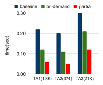
(a) EPL, 47K BGP matches

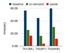
(b) Email, 862K BGP matches

Figure 9: Running time for path of length 2 with timed automata $\mathit{TA}_{1},\mathit{TA}_{2},\mathit{TA}_{3}$.

Table 2: Relative performance of baseline, on-demand and partial-match, for different BGPs and automaton $\mathit{TA}_{0}$.

EPL	# of matches		time (sec)
pattern	BGP	BGP+TA	match	baseline	on-demand	partial
path2	47K	1.8K	0.01	0.22	0.12	0.06
path3	1.5M	4.6K	0.21	5.11	3.66	0.32
cycle2	1.1K	35	0.01	0.03	0.01	0.02
cycle3	35K	66	0.02	0.12	0.09	0.36
cycle4	1.1M	106	0.22	3.31	2.92	0.53
Email	# of matches		time (sec)
pattern	BGP	BGP+TA	match	baseline	on-demand	partial
path2	862K	36K	0.25	56.27	25.56	16.35
path3	42M	126K	41	1475.20	766.33	74.77
cycle2	18K	843	0.12	0.92	0.54	2.41
cycle3	205K	309	0.19	5.13	3.49	14.34
cycle4	8.4M	1352	4.38	196.50	125.85	92.40
Contact	# of matches		time (sec)
pattern	BGP	BGP+TA	match	baseline	on-demand	partial
I-Star2	10.1K	0	0.01	0.03	0.03	0.01
O-Star2	207K	0	0.03	0.84	0.79	0.67
I-Star3	21.4K	0	0.01	0.07	0.06	0.03
O-Star3	10.7M	0	2.86	36.24	35.26	1.73
FB-wall	# of matches		time (sec)
pattern	BGP	BGP+TA	match	baseline	on-demand	partial
path2	4.4M	681K	1.08	839.30	387.31	318.14
path3	91M	235K	13.44	9477.47	5093.05	998.54
cycle2	160K	16K	0.94	12.34	8.32	66.76
cycle3	272K	4.1K	0.84	17.69	10.94	341.39

Figure  9 shows the execution time of the baseline, on-demand and partial-match algorithms for EPL and Email, also noting the number of temporal matches. The BGP, which is in common for all executions in this experiment, returns 47K matches on EPL and 862K matches on Email. When the temporal constraint is applied, the number of matches is reduced, and is presented on the $x$-axis. For example, $\mathit{TA}_{1}$ returns 1.8K matches on EPL and 36K on Email.

We observe that partial-match is the most efficient algorithm for all queries and both datasets, returning in under 0.12 sec for EPL, and in under 17 sec for Email in all cases. The on-demand algorithm outperforms the baseline in all cases, but is slower than partial-match. The performance difference between the baseline and on-demand is due to a join between two large relations in baseline, compared to multiple joins over smaller relations in on-demand.

We also observe that the relative performance of the algorithms depends on the number of matches, and explore this relationship further in the next experiment. To compare algorithm performance across different BGPs and datasets, we use the timed automaton $\mathit{TA}_{0}$ of Figure 8, which generalizes $\mathit{TA}_{1}$ from $2$ to $m$ edges. $\mathit{TA}_{0}$ specifies that edges in a matching should appear repeatedly in a strict temporal order. We use $\mathit{TA}_{0}$ (with $m=2$, 3, or 4 as appropriate) as the temporal constraint for paths of length 2 and 3, and for cycles of length 2, 3, 4, for three of the datasets. Because the Contact dataset is a bipartite graph, we used it for in-star ($x_{2}\xrightarrow{y_{1}}x_{1}\xleftarrow{y_{2}}x_{3}$) and out-star($x_{2}\xleftarrow{y_{1}}x_{1}\xrightarrow{y_{2}}x_{3}$) BGPs of size 2 and 3.

Table 2 summarizes the results. It shows number of BGP matchings (“BGP”), number of matchings accepted by $\mathit{TA}_{0}$ (“BGP+TA”), and running times of computing the BGP match only (“match”), and of computing both BGP and temporal matches using to the baseline, on-demand, and partial-match algorithms.

We observe that, for acylic patterns (e.g., paths, i-star, o-star), partial-match is significantly faster than on-demand and baseline. For such patterns, partial matchings are shared by many total matchings and by larger partial matchings, benefiting the running time. Interestingly, for cycles of size 2 and 3, on-demand is fastest, followed by baseline. However, for cycles of size 4 partial-match is once again the fastest algorithm. The reason for this is that there are far fewer cycles than possible partial matchings, and in smaller cycles this causes partial-match to run slower. As cycle size increases, performance of partial-match becomes comparable to, or better, than of the other two algorithms. Another graph characteristic that can affect partial-match performance is graph density, which we discuss in the next section. (Our machine’s RAM could not fit cycle4 for FB-Wall, so we did not conduct that experiment.)

6.2 Comparison to in-memory databases

In this set of experiments, we compare the running time of temporal BGP matching with equivalent relational queries. We used three datasets (EPL, Contact and Email) and queried them with cyclic and acyclic BGPs of size 2, with temporal constraints specified by 9 timed automata: $TA_{e}$ specifies an existential constraint (Figure 3), while $TA_{1}\ldots TA_{8}$ express constraints that are not existential.

We showed SQL queries QTA1 and QTA7 in the introduction. In the Supplementary Materials we give a complete listing of the SQL queries, with Path2, Cycl2 and Star2 expressing the BGPs used in our experiments, and QTAE, QTA1–QTA8 implementing the temporal constraints. Most of these queries are quite complicated compared to their equivalent timed automata.

For DuckDB and HyPer, we loaded the relations Node, Edge and Active into memory. To improve performance of DuckDB, we defined indexes on Edge(src), Edge(dst), and Active(eid,time). To the best of our knowledge, HyPer does not support indexes.

Table 3 shows the execution time for each query, comparing the running time of the best method based on timed automata (on-demand or partial-match, column “TAA”) with DuckDB and HyPer. Observe that our algorithms are significantly faster for $\mathit{TA}_{1}$, $\mathit{TA}_{2}$, $\mathit{TA}_{5}$ and $\mathit{TA}_{7}$ for all 3 datasets, and have comparable performance to the best-performing relational system for $\mathit{TA}_{3}$ and $\mathit{TA}_{4}$. Relational systems outperform our algorithms on $\mathit{TA}_{e}$ and $\mathit{TA}_{6}$. For $\mathit{TA}_{e}$, relational databases compute all possible matchings at all the time points in one shot, and then filter out those that fail the temporal constraint, which can be faster than an iterative process. Similarly, for $\mathit{TA}_{6}$, the XOR operator can be implemented as a join-antijoin. Interestingly, for $\mathit{TA}_{8}$ (set containment join, see Introduction) DuckDB is most efficient, followed by our algorithms, and then by HyPer. For the majority of other cases, DuckDB either ran out of memory (OM in Table 3) or was the slowest system. Results for EPL are in supplementary materials.Note that our system was able to handle all queries within the allocated memory, with DuckDB and HyPer both ran out of memory in some cases.

6.3 Impact of graph properties on performance

Table 3: Best-performing timed-automaton algorithm (TAA) compared to DuckDB and HyPer, for SQL queries in Figure 3.

		time (sec)
EPL Path2	TA	# matches	TAA	DuckDB	HyPer
	$\mathit{TA}_{e}$	35866	1.09	1.11	1.44
	$\mathit{TA}_{1}$	1801	0.06	60.14	17.84
	$\mathit{TA}_{2}$	374	0.05	69.89	11.36
	$\mathit{TA}_{3}$	21035	0.04	0.07	0.13
	$\mathit{TA}_{4}$	29726	0.06	0.07	0.13
	$\mathit{TA}_{5}$	1714	0.07	18.57	0.39
	$\mathit{TA}_{6}$	19578	0.54	0.12	0.09
	$\mathit{TA}_{7}$	257	1.3	8.22	5.56
	$\mathit{TA}_{8}$	5377	0.23	0.17	0.21
EPL Cycle2	$\mathit{TA}_{e}$	933	0.04	0.597	0.01
	$\mathit{TA}_{1}$	35	0.01	2.67	0.41
	$\mathit{TA}_{2}$	22	0.01	3.33	0.26
	$\mathit{TA}_{3}$	418	0.01	0.1	0.01
	$\mathit{TA}_{4}$	740	0.01	0.1	0.01
	$\mathit{TA}_{5}$	90	0.02	0.53	1.19
	$\mathit{TA}_{6}$	312	0.07	0.07	0.01
	$\mathit{TA}_{7}$	0	0.05	1.18	5.15
	$\mathit{TA}_{8}$	188	0.02	0.01	0.09
Contact O-Star2	$\mathit{TA}_{e}$	169410	8.87	22.43	19.29
	$\mathit{TA}_{1}$	0	0.67	OM	316.5
	$\mathit{TA}_{2}$	0	0.72	OM	205.95
	$\mathit{TA}_{3}$	101268	0.59	0.95	0.69
	$\mathit{TA}_{4}$	107650	0.68	0.91	0.68
	$\mathit{TA}_{5}$	4154	0.72	OM	2.035
	$\mathit{TA}_{6}$	10832	4.68	0.99	0.54
	$\mathit{TA}_{7}$	76	15.12	OM	102.89
	$\mathit{TA}_{8}$	4646	1.3	1.1	1.16
Email Path2	$\mathit{TA}_{e}$	719609	501.07	649.69	239.82
	$\mathit{TA}_{1}$	35594	22.35	OM	OM
	$\mathit{TA}_{2}$	801	3.73	OM	1748.85
	$\mathit{TA}_{3}$	443431	7.78	17.84	8.59
	$\mathit{TA}_{4}$	455977	7.82	17.78	8.26
	$\mathit{TA}_{5}$	2474	1.27	OM	48.87
	$\mathit{TA}_{6}$	693956	320.04	8.98	5.61
	$\mathit{TA}_{7}$	390	327.33	OM	OM
	$\mathit{TA}_{8}$	12919	19.32	8.02	21.58
Email Cycle2	$\mathit{TA}_{e}$	14188	4.71	254.7	15.3
	$\mathit{TA}_{1}$	843	0.83	OM	1788.87
	$\mathit{TA}_{2}$	240	0.64	OM	1733.05
	$\mathit{TA}_{3}$	6333	0.46	0.38	0.68
	$\mathit{TA}_{4}$	11396	0.44	0.38	0.68
	$\mathit{TA}_{5}$	1800	0.97	206.26	1.19
	$\mathit{TA}_{6}$	4230	24.09	8.63	5.48
	$\mathit{TA}_{7}$	134	7.1	OM	OM
	$\mathit{TA}_{8}$	3441	1.79	0.219	49.79

In this set of experiments, we explore the effect of structural density and temporal domain size. We synthetically generated a complete graph with 50 nodes and 2450 edges (the same size as the EPL dataset) and temporal density of $0.5$. We then sampled edges to create a graph with different structural densities. We use 4 representative BGPs: paths of length 3, and cycles of length 3. As temporal constraint we use $\mathit{TA}_{4}$ from Figure 8, as it has low early rejection rate, thus serving as a worst case.

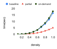
(a) path 3

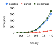
(b) path 4

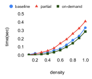
(c) cycle 3

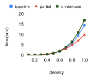
(d) cycle 4

Figure 10: Running time as a function of structural density for 4 common BGPs, with timed automaton $\mathit{TA}_{4}$ in Figure 8.

Figure 10 shows the execution time of each algorithm as a function of graph density, varying from 0.1 to 1.0, where density 1.0 corresponds to a complete graph. Observe that partial-match outperforms on-demand for paths, particularly as graph density increases. For the cycle of size 3, baseline and on-demand have better performance than partial-match, but the performance gap decreases with increasing graph density. Our experiments for BGPs: path of length 4 and cycle of length 4 show similar trend. Notably, performance of on-demand is very close to the baseline.

Next, we consider the impact of temporal domain size on performance. In general, we expect execution times to increase with increasing temporal domain size. To measure this effect without changing the structure or the size of the graph, we synthetically changed the temporal resolution of the Email dataset, creating graphs with between 25 and 800 snapshots, and thus keeping the number of BGP matchings fixed.

Figure 11a shows the result of executing temporal BGP with path of length 2 and time automaton $\mathit{TA}_{1}$ (Figure 2b). Observe that the execution time of all algorithms increases linearly, with partial-match scaling best with increasing number of snapshots.

Finally, we study the relationship between result set size of a temporal BGP and algorithm performance. For this, we executed the path of length 2 BGP on the Email dataset, with timed automaton $\mathit{TA}_{2}$ in Figure 2c, and manipulated selectivity by varying the clock condition from $c<0$ to $c<1024$ on the logarithmic scale. With these settings, the temporal BGP accepts between 0 and 36K matchings. Figure 11b presents the result of this experiment, showing the running time (in sec) on the $x$-axis and the number of temporal BGP matchings (in thousands) on the $y$-axis. Observe that the running time increases linearly with increasing number of accepted matchings for all algorithms, and the slope of increase is small.

6.4 Impact of the number of clocks and automaton size on performance

In our final set of experiments, we investigate the impact of automaton size and of the number of clocks on performance, while keeping all other parameters fixed to the extent possible. To do this, we fix the BGP and vary the size of the automaton, as follows. We fix the BGP to cycle4 and take $\mathit{TA}_{0}$ (Figure 8) with $m=4$ as a starting point. We can unfold the cycle of states, thus doubling the number of states but resulting in an equivalent automaton. We do this doubling seven times, until we obtain 256 states.

Figure 12a shows the execution times on the EPL dataset. Observing that the execution times remain constant, we conclude that automaton size does not significantly impact performance.

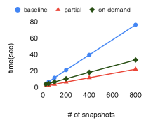
(a) path2 with $\mathit{TA}_{1}$ on Email

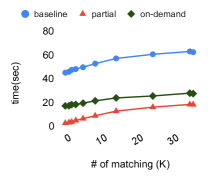
(b) path2 with $\mathit{TA}_{2}$ on Email

Figure 11: (a) running time vs. temporal domain size; (b) relationship between running time and result set size.

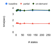
(a) # states

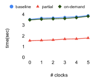
(b) # clocks

Figure 12: Running time as a function of automaton size for cycle of size 4 with $\mathit{TA}_{0}$ (Figure 8) on EPL.

Finally, to investigate the impact of the number of clocks on performance, we added multiple clocks to the automaton in Figure 8 and we reset all clocks at every state transition. To ensure that any possible difference is not due to the change of output size, the condition of each clock is set to $\mathit{true}$. Figure 12b shows the result of this experiment, with the number of clocks on the $x$-axis and the execution time in seconds on the $y$-axis. Observe that the running time of all algorithms increases very slightly with increasing number of clocks. We thus conclude that the computational overhead of storing and updating clocks is low.

7 Related Work

During the past several decades, researchers considered different aspects of graph pattern matching, see Conte et al. conte2004thirty for a survey. The majority of temporal graph models use either time points DBLP:conf/sigmod/GurukarRR15 ; DBLP:journals/corr/abs-1107-5646 ; DBLP:conf/wsdm/ParanjapeBL17 or intervals DBPL2017 ; xu2017time ; DBLP:conf/edbt/ZufleREF18 ; rost2022distributed to enrich graphs with temporal information. In our work, we associate each edge in a graph with a set of time points, which is an appropriate representation when events — such as messages between users or citations — are instantaneous and so do not have a duration. It is an interesting topic for further research to investigate when and how an interval-based approach can be encoded by a point-based approach. This depends also on the considered graph model, and the considered class of queries and temporal constraints.

A prominent line of work where the point-based approach is adopted is that of mining frequent temporal subgraphs, called temporal motifs DBLP:conf/sigmod/GurukarRR15 ; DBLP:journals/corr/abs-1107-5646 ; DBLP:conf/wsdm/ParanjapeBL17 . There, the focus is typically on existential temporal constrains, aiming to identify graph patterns with a specific temporal order among the edges, such as in our Example 1. Timed automata can easily specify such constrains. An important type of a motif is a $\delta$ temporal motif DBLP:conf/wsdm/ParanjapeBL17 , where all the edges occur inside the period of $\delta$ time units. Timed automata can use one or multiple clocks to enforce such constrains.

Züfle et al. DBLP:conf/edbt/ZufleREF18 consider a particular class of temporal constraints where the time points within a query range are specified exactly up to the translation of the query range into the temporal range of the graph. Such constraints are more general than existential constraints, in that they can represent gaps. An interesting aspect of this work is that the history of each subgraph is represented as a string, and the temporal constraint is checked using substring search. While this method of expressing constraints can work over a set of time points, it is limited to ordered temporal constraints and does not support reoccurring edges.

There are various lines of research on querying temporal graphs that are complementary to our focus in this paper. For example, durable matchings semertzidis2016durable ; li2022durable count the number of snapshots in which a matching exists. Much attention has also been paid to tracing unbounded paths in temporal graphs, under various semantics, e.g., fastest, earliest arrival, latest departure, time-forward, time travel, or continuous DBLP:journals/tkde/ByunWK20 ; Debrouvier21 ; DBLP:conf/sigmod/JohnsonKLS16 ; DBLP:journals/pvldb/WuCHKLX14 ; DBLP:journals/tkde/WuCKHHW16 ; DBLP:conf/icde/WuHCLK16 . A focus on unbounded paths is complementary to our work on patterns without path variables, but with powerful temporal constraints. Extending our framework with path variables is an interesting direction for further research.

An important aspect of pattern matching in graphs is efficiently extracting the matchings. Early work started with the back-tracking algorithm by Ullmann ullmann1976algorithm , with later improvements vcibej2015improvements ; ulman2011 . Pruning strategies for brute-force algorithms have been investigated as well DBLP:journals/pami/CarlettiFSV18 ; cordella1999performance ; cordella2004sub . Approaches suitable for large graphs typically build up the set of matchings in a relational table lai2019distributed by a series of natural joins over the edge relation; the aim is then to find an optimal join order. Until recently, the best-performing approaches were based on edge-growing pairwise join plans DBLP:journals/pvldb/LaiQLC15 ; selinger1989access ; DBLP:journals/pvldb/SunWWSL12 , but a new family of vertex-growing plans, known as worst-case optimal joins, have emerged arroyuelo2021worst ; DBLP:journals/sigmod/NgoRR13 ; DBLP:journals/corr/abs-1210-0481 , with better performance for cyclic patterns such as triangles. While we use the latter approach and implement our algorithms using relational operators, any method capable of finding matchings on a static graph can be combined with our timed automaton-based algorithms.

Another relevant direction is incremental graph pattern matching amsj_subgraph ; DBLP:conf/eurosys/BindschaedlerML21 ; DBLP:journals/tkde/ChenW10 ; fan2013incremental ; DBLP:conf/sigmod/HanLL13 ; imran2022fast ; DBLP:conf/sigmod/KimSHLHCSJ18 ; DBLP:conf/sigmod/KoLHLSSH21 , where the goal is to find and maintain patterns in an updating graph.

8 Conclusions and Future Work

In this paper, we proposed to use timed automata as a simple but powerful formalism for specifying temporal constraints in temporal graph pattern matching. We introduced algorithms that retrieve all temporal BGP matchings in a large graph, and presented results of an experimental evaluation, showing that this approach is practical, and identifying interesting performance trade-offs. Our code and data are available at http://github.com/amirpouya/TABGP.

An interesting open problem is how timed automata exactly compare to SQL in expressing temporal constraints (pinpointing the expressive power of SQL on ordered data is notoriously hard libkin_sql ). It is also interesting to investigate the decidability and complexity of the containment problem for temporal BGPs based on timed automata. Another natural direction for further research is to adapt our framework to a temporal graph setting where edges are active at durations (intervals), rather than at separate timepoints. Our hypothesis is that we can encode any set of non-overlapping intervals by the set of border-points. We conjecture that timed automata under such an encoding can express common constraints on intervals, such as Allen’s relations allen1983maintaining .

Appendix A Supplementary materials for Section 6

Figure 13: Version of $\mathit{TA}_{4}$ for two edge variables.

We present the SQL queries for the temporal BGPs with timed automata used in the experiments. For this experiment, we used BGPs with two edge variables. Thus, $\mathit{TA}_{4}$, originally shown in Figure 8, is adapted here to two edge variables, as shown in Figure 13.

⬇

Path2: SELECT E1.eid AS y1, E2.eid AS y2 FROM edge E1, edge AS E2 WHERE E1.dst = E2.src

Cycl2: SELECT E1.eid AS y1, E2.eid AS y2 FROM edge E1, edge AS E2 WHERE E1.dst = E2.src and E2.dst = E1.src

Star2: SELECT E1.eid AS y1, E2.eid AS y2 FROM edge E1, edge AS E2 WHERE E1.dst = E2.dst

⬇

QTAE: SELECT M.y1, M.y2 FROM matching M, active A1,active A2

WHERE M.y1 = A1.eid AND M.y2 = A2.eidand A1.time < A2.time

⬇

QTA1: WITH matching(y1,y2) as (...),

Succ AS

(SELECT y1, y2, A1.eid AS e1, A2.eid AS e2

FROM matching, active A1, active A2

WHERE (A1.eid = y1 OR A1.eid = y2) AND (A2.eid = y1 OR A2.eid = y2)

AND A1.time<A2.time AND NOT EXISTS

(SELECT * FROM active A3

WHERE (A3.eid = y1 or A3.eid = y2)

AND A1.time<A3.time AND A3.time<A2.time))

SELECT * FROM matching M

WHERE NOT ( EXISTS (SELECT * FROM active WHERE eid = y2)

AND NOT EXISTS (SELECT * FROM active WHERE eid = y1) )

AND ( NOT EXISTS (SELECT * FROM active A1, active A2

WHERE A1.eid = y1 AND A2.eid = y2)

OR (SELECT MIN(time) FROM active WHERE eid = y1) <

(SELECT MIN(time) FROM active WHERE eid = y2) )

AND NOT EXISTS (SELECT * FROM Succ

WHERE M.y1 = y1 AND M.y2 = y2 AND e1 = e2);

⬇

QT2: WITH matching(y1, y2) AS (...),

Succ AS

(SELECT y1, y2, A1.eid as e1, A2.eid as e2, A1.time as t1, A2.time as t2

FROM matching, active A1, active A2

WHERE (A1.eid = y1 OR A1.eid = y2) AND (A2.eid = y1 OR A2.eid = y2)

AND A1.time<A2.time AND NOT EXISTS

(SELECT * FROM active A3

WHERE (A3.eid = y1 or A3.eid = y2)

AND A1.time<A3.time AND A3.time<A2.time))

SELECT * FROM matching M

WHERE NOT ( EXISTS (SELECT * FROM active WHERE eid = y2)

AND NOT EXISTS (SELECT * FROM active WHERE eid = y1) )

AND ( NOT EXISTS (SELECT * FROM active A1, active A2

WHERE A1.eid = y1 AND A2.eid = y2)

OR (SELECT MIN(time) FROM active WHERE eid = y1) <

(SELECT MIN(time) FROM active WHERE eid = y2) )

AND NOT EXISTS (SELECT * FROM Succ

WHERE M.y1 = y1 AND (e1 = e2 OR t2 - t1 >= 3)

⬇

QTA3: WITH matching(y1, y2) AS (...)

SELECT M.y1, M.y2 FROM Matching M, active A1, active A2

WHERE M.y1 = A1.eid AND M.y2 = A2.eid

GROUP BY M.y1, M.y2 HAVING MIN(A1.time) < MIN(A2.time)

⬇

QTA4: WITH matching(y1, y2) AS (...)

SELECT M.y1, M.y2 FROM Matching M, active A1, active A2

WHERE M.y1 = A1.eid AND M.y2 = A2.eid

GROUP BY M.y1, M.y2 HAVING MIN(A1.time) <= MIN(A2.time)

⬇

QTA5: WITH matching(y1, y2) AS (...)

SELECT * FROM Matching WHERE NOT EXISTS

(SELECT * FROM active WHERE

(time IN (SELECT time FROM active WHERE eid = y1)

OR time IN (SELECT time FROM active WHERE eid = y2))

AND (time NOT IN (SELECT time FROM active WHERE eid = y1)

OR time NOT IN (SELECT time FROM active WHERE eid = y2)))

⬇

QTA6: WITH matching(y1, y2) AS (...)

SELECT * FROM matching WHERE NOT EXISTS

(SELECT * FROM active A1, active A2

WHERE A1.eid = y1 AND A2.eid = y2 AND A1.time = A2.time)

⬇

QTA7: WITH matching AS (...)

SELECT DISTINCT y1, y2

FROM matching, active A1, active A2, active B1, active B2

WHERE A1.eid = y1 AND A2.eid = y2 AND A1.time = A2.time

AND B1.eid = y1 AND B2.eid = y2 AND B1.time = B2.time

AND B1.time - A1.time > 3

AND NOT EXISTS

(SELECT * FROM active C

WHERE A1.time < C.time AND C.time < B1.time

AND NOT EXISTS (SELECT * FROM active C1, active C2

WHERE C1.time = C.time AND C2.time = C.time

AND C1.eid = y1 AND C2.eid = y2));

⬇

QTA8: WITH matching(y1, y2) AS (...)

SELECT * FROM Matching WHERE NOT EXISTS

(SELECT * FROM active WHERE eid = y1 AND time NOT IN

(SELECT time FROM active WHERE eid = y2))

References

- (1) Allen, J.F.: Maintaining knowledge about temporal intervals. Communications of the ACM 26(11), 832–843 (1983)
- (2) Alur, R., Dill, D.: A theory of timed automata. Theoretical Computer Science 126, 183–235 (1994)
- (3) Ammar, K., McSherry, F., Salihoglu, S., Joglekar, M.: Distributed evaluation of subgraph queries using worst-case optimal low-memory dataflows. PVLDB 11(6), 691–704 (2018)
- (4) Angles, R., Arenas, M., Barceló, P., Hogan, A., Reutter, J.L., Vrgoc, D.: Foundations of modern query languages for graph databases. ACM Comput. Surv. 50(5), 68:1–68:40 (2017). DOI 10.1145/3104031. URL http://doi.acm.org/10.1145/3104031
- (5) Arroyuelo, D., Hogan, A., Navarro, G., Reutter, J.L., Rojas-Ledesma, J., Soto, A.: Worst-case optimal graph joins in almost no space. In: SIGMOD (2021)
- (6) Bindschaedler, L., Malicevic, J., Lepers, B., Goel, A., Zwaenepoel, W.: Tesseract: distributed, general graph pattern mining on evolving graphs. In: A. Barbalace, P. Bhatotia, L. Alvisi, C. Cadar (eds.) EuroSys ’21: Sixteenth European Conference on Computer Systems, Online Event, United Kingdom, April 26-28, 2021, pp. 458–473. ACM (2021). DOI 10.1145/3447786.3456253. URL https://doi.org/10.1145/3447786.3456253
- (7) Bouros, P., Mamoulis, N., et al.: Set containment join revisited. Knowledge and Information Systems 49, 375–402 (2016)
- (8) Bouyer, P., Fahrenberg, U., K., G.L., Markey, N., Ouaknine, J., Worell, J.: Model checking real-time systems. In: E. Clarke, T. Henzinger, H. Veith, et al. (eds.) Handbook of Model Checking, pp. 1001–1046. Springer (2018)
- (9) Byun, J., Woo, S., Kim, D.: Chronograph: Enabling temporal graph traversals for efficient information diffusion analysis over time. IEEE Trans. Knowl. Data Eng. 32(3), 424–437 (2020). DOI 10.1109/TKDE.2019.2891565. URL https://doi.org/10.1109/TKDE.2019.2891565
- (10) Carbone, P., Katsifodimos, A., Ewen, S., Markl, V., Haridi, S., Tzoumas, K.: Apache flink: Stream and batch processing in a single engine. Bulletin of the IEEE Computer Society Technical Committee on Data Engineering 36(4) (2015)
- (11) Carletti, V., Foggia, P., Saggese, A., Vento, M.: Challenging the time complexity of exact subgraph isomorphism for huge and dense graphs with VF3. IEEE Trans. Pattern Anal. Mach. Intell. 40(4), 804–818 (2018). DOI 10.1109/TPAMI.2017.2696940. URL https://doi.org/10.1109/TPAMI.2017.2696940
- (12) Chen, L., Wang, C.: Continuous subgraph pattern search over certain and uncertain graph streams. IEEE Trans. Knowl. Data Eng. 22(8), 1093–1109 (2010). DOI 10.1109/TKDE.2010.67. URL https://doi.org/10.1109/TKDE.2010.67
- (13) Cheng, J., Yu, J.X., Ding, B., Philip, S.Y., Wang, H.: Fast graph pattern matching. In: 2008 IEEE 24th International Conference on Data Engineering, pp. 913–922. IEEE (2008)
- (14) Čibej, U., Mihelič, J.: Improvements to ullmann’s algorithm for the subgraph isomorphism problem. International Journal of Pattern Recognition and Artificial Intelligence 29(07), 1550,025 (2015)
- (15) Conte, D., Foggia, P., Sansone, C., Vento, M.: Thirty years of graph matching in pattern recognition. International journal of pattern recognition and artificial intelligence 18(03), 265–298 (2004)
- (16) Cordella, L.P., Foggia, P., Sansone, C., Vento, M.: Performance evaluation of the vf graph matching algorithm. In: Proceedings 10th International Conference on Image Analysis and Processing, pp. 1172–1177. IEEE (1999)
- (17) Cordella, L.P., Foggia, P., Sansone, C., Vento, M.: A (sub) graph isomorphism algorithm for matching large graphs. IEEE transactions on pattern analysis and machine intelligence 26(10), 1367–1372 (2004)
- (18) Curley, J.: Engsoccerdata: English soccer data 1871-2106. R Package Version 0.1 5 (2016)
- (19) Debrouvier, A., Parodi, E., Perazzo, M., Soliani, V., Vaisman, A.: A model and query language for temporal graph databases. VLDB Journal 30(5) (2021). DOI https://doi.org/10.1007/s00778-021-00675-4
- (20) Fan, W., Li, J., Ma, S., Tang, N., Wu, Y., Wu, Y.: Graph pattern matching: from intractable to polynomial time. Proceedings of the VLDB Endowment 3(1-2), 264–275 (2010)
- (21) Fan, W., Wang, X., Wu, Y.: Incremental graph pattern matching. ACM Transactions on Database Systems (TODS) 38(3), 1–47 (2013)
- (22) Grez, A., Riveros, C., Ugarte, M., Vansummeren, S.: A formal framework for complex event recognition. TODS 46(4) (2021)
- (23) Gupta, A., Mumick, I.S., Subrahmanian, V.S.: Maintaining views incrementally. ACM SIGMOD Record 22(2), 157–166 (1993)
- (24) Gurukar, S., Ranu, S., Ravindran, B.: COMMIT: A scalable approach to mining communication motifs from dynamic networks. In: T.K. Sellis, S.B. Davidson, Z.G. Ives (eds.) Proceedings of the 2015 ACM SIGMOD International Conference on Management of Data, Melbourne, Victoria, Australia, May 31 - June 4, 2015, pp. 475–489. ACM (2015). DOI 10.1145/2723372.2737791. URL https://doi.org/10.1145/2723372.2737791
- (25) Han, W., Lee, J., Lee, J.: Turbo: towards ultrafast and robust subgraph isomorphism search in large graph databases. In: K.A. Ross, D. Srivastava, D. Papadias (eds.) Proceedings of the ACM SIGMOD International Conference on Management of Data, SIGMOD 2013, New York, NY, USA, June 22-27, 2013, pp. 337–348. ACM (2013). DOI 10.1145/2463676.2465300. URL https://doi.org/10.1145/2463676.2465300
- (26) Imran, M., Gévay, G.E., Quiané-Ruiz, J.A., Markl, V.: Fast datalog evaluation for batch and stream graph processing. World Wide Web (2022)
- (27) Johnson, T., Kanza, Y., Lakshmanan, L.V.S., Shkapenyuk, V.: Nepal: a path query language for communication networks. In: A. Arora, S. Roy, S. Mehta (eds.) Proceedings of the 1st ACM SIGMOD Workshop on Network Data Analytics, NDA@SIGMOD 2016, San Francisco, California, USA, July 1, 2016, pp. 6:1–6:8. ACM (2016). DOI 10.1145/2980523.2980530. URL https://doi.org/10.1145/2980523.2980530
- (28) Kim, K., Seo, I., Han, W., Lee, J., Hong, S., Chafi, H., Shin, H., Jeong, G.: Turboflux: A fast continuous subgraph matching system for streaming graph data. In: G. Das, C.M. Jermaine, P.A. Bernstein (eds.) Proceedings of the 2018 International Conference on Management of Data, SIGMOD Conference 2018, Houston, TX, USA, June 10-15, 2018, pp. 411–426. ACM (2018). DOI 10.1145/3183713.3196917. URL https://doi.org/10.1145/3183713.3196917
- (29) Ko, S., Lee, T., Hong, K., Lee, W., Seo, I., Seo, J., Han, W.: iturbograph: Scaling and automating incremental graph analytics. In: G. Li, Z. Li, S. Idreos, D. Srivastava (eds.) SIGMOD ’21: International Conference on Management of Data, Virtual Event, China, June 20-25, 2021, pp. 977–990. ACM (2021). DOI 10.1145/3448016.3457243. URL https://doi.org/10.1145/3448016.3457243
- (30) Kovanen, L., Karsai, M., Kaski, K., Kertész, J., Saramäki, J.: Temporal motifs in time-dependent networks. CoRR abs/1107.5646 (2011). URL http://arxiv.org/abs/1107.5646
- (31) Lai, L., Qin, L., Lin, X., Chang, L.: Scalable subgraph enumeration in mapreduce. Proc. VLDB Endow. 8(10), 974–985 (2015). DOI 10.14778/2794367.2794368. URL http://www.vldb.org/pvldb/vol8/p974-lai.pdf
- (32) Lai, L., Qing, Z., Yang, Z., Jin, X., Lai, Z., Wang, R., Hao, K., Lin, X., Qin, L., Zhang, W., et al.: Distributed subgraph matching on timely dataflow. Proceedings of the VLDB Endowment 12(10), 1099–1112 (2019)
- (33) Leskovec, J., Kleinberg, J.M., Faloutsos, C.: Graph evolution: Densification and shrinking diameters. TKDD 1(1), 2 (2007). DOI 10.1145/1217299.1217301. URL http://doi.acm.org/10.1145/1217299.1217301
- (34) Li, F., Zou, Z., Li, J.: Durable subgraph matching on temporal graphs. IEEE Transactions on Knowledge and Data Engineering (2022)
- (35) Libkin, L.: Expressive power of SQL. Theoretical Computer Science 296, 379–404 (2003)
- (36) McSherry, F., Murray, D.G., Isaacs, R., Isard, M.: Differential dataflow. In: CIDR (2013)
- (37) Moffitt, V.Z., Stoyanovich, J.: Temporal graph algebra. In: Proceedings of The 16th International Symposium on Database Programming Languages, DBPL 2017, Munich, Germany, September 1, 2017, pp. 10:1–10:12 (2017). DOI 10.1145/3122831.3122838. URL http://doi.acm.org/10.1145/3122831.3122838
- (38) Moffitt, V.Z., Stoyanovich, J.: Temporal graph algebra. In: Proceedings of The 16th International Symposium on Database Programming Languages, DBPL 2017, Munich, Germany, September 1, 2017, pp. 10:1–10:12 (2017). DOI 10.1145/3122831.3122838. URL http://doi.acm.org/10.1145/3122831.3122838
- (39) Murray, D.G., McSherry, F., Isaacs, R., Isard, M., Barham, P., Abadi, M.: Naiad: a timely dataflow system. In: Proceedings of the Twenty-Fourth ACM Symposium on Operating Systems Principles, pp. 439–455 (2013)
- (40) Neumann, T.: Efficiently compiling efficient query plans for modern hardware. Proc. VLDB Endow. 4(9), 539–550 (2011). DOI 10.14778/2002938.2002940. URL http://www.vldb.org/pvldb/vol4/p539-neumann.pdf
- (41) Neumann, T., Mühlbauer, T., Kemper, A.: Fast serializable multi-version concurrency control for main-memory database systems. In: T.K. Sellis, S.B. Davidson, Z.G. Ives (eds.) Proceedings of the 2015 ACM SIGMOD International Conference on Management of Data, Melbourne, Victoria, Australia, May 31 - June 4, 2015, pp. 677–689. ACM (2015). DOI 10.1145/2723372.2749436. URL https://doi.org/10.1145/2723372.2749436
- (42) Ngo, H.Q., Ré, C., Rudra, A.: Skew strikes back: new developments in the theory of join algorithms. SIGMOD Rec. 42(4), 5–16 (2013). DOI 10.1145/2590989.2590991. URL https://doi.org/10.1145/2590989.2590991
- (43) Ojagh, S., Saeedi, S., Liang, S.H.: A person-to-person and person-to-place covid-19 contact tracing system based on ogc indoorgml. ISPRS International Journal of Geo-Information 10(1), 2 (2021)
- (44) Paranjape, A., Benson, A.R., Leskovec, J.: Motifs in temporal networks. In: M. de Rijke, M. Shokouhi, A. Tomkins, M. Zhang (eds.) Proceedings of the Tenth ACM International Conference on Web Search and Data Mining, WSDM 2017, Cambridge, United Kingdom, February 6-10, 2017, pp. 601–610. ACM (2017). DOI 10.1145/3018661.3018731. URL https://doi.org/10.1145/3018661.3018731
- (45) Raasveldt, M., Mühleisen, H.: Duckdb: an embeddable analytical database. In: P.A. Boncz, S. Manegold, A. Ailamaki, A. Deshpande, T. Kraska (eds.) Proceedings of the 2019 International Conference on Management of Data, SIGMOD Conference 2019, Amsterdam, The Netherlands, June 30 - July 5, 2019, pp. 1981–1984. ACM (2019). DOI 10.1145/3299869.3320212. URL https://doi.org/10.1145/3299869.3320212
- (46) Reza, T., Ripeanu, M., Sanders, G., Pearce, R.: Approximate pattern matching in massive graphs with precision and recall guarantees. In: Proceedings of the 2020 ACM SIGMOD International Conference on Management of Data, pp. 1115–1131 (2020)
- (47) Rost, C., Gomez, K., Täschner, M., Fritzsche, P., Schons, L., Christ, L., Adameit, T., Junghanns, M., Rahm, E.: Distributed temporal graph analytics with gradoop. The VLDB Journal 31(2), 375–401 (2022)
- (48) Rust-Itertools: rust-itertools/itertools. URL https://github.com/rust-itertools/itertools
- (49) Selinger, P.G., Astrahan, M.M., Chamberlin, D.D., Lorie, R.A., Price, T.G.: Access path selection in a relational database management system. In: Readings in Artificial Intelligence and Databases, pp. 511–522. Elsevier (1989)
- (50) Semertzidis, K., Pitoura, E.: Durable graph pattern queries on historical graphs. In: 2016 IEEE 32nd International Conference on Data Engineering (ICDE), pp. 541–552. IEEE (2016)
- (51) Sun, Z., Wang, H., Wang, H., Shao, B., Li, J.: Efficient subgraph matching on billion node graphs. Proc. VLDB Endow. 5(9), 788–799 (2012). DOI 10.14778/2311906.2311907. URL http://vldb.org/pvldb/vol5/p788_zhaosun_vldb2012.pdf
- (52) Ullmann, J.R.: An algorithm for subgraph isomorphism. Journal of the ACM (JACM) 23(1), 31–42 (1976)
- (53) Ullmann, J.R.: Bit-vector algorithms for binary constraint satisfaction and subgraph isomorphism. Journal of Experimental Algorithmics 15, 1.6:1–1.6:64 (2011). DOI 10.1145/1671970.1921702
- (54) Veldhuizen, T.L.: Leapfrog triejoin: a worst-case optimal join algorithm. In: Proceedings 17th International Conference on Database Theory, pp. 96–106 (2014)
- (55) Viswanath, B., Mislove, A., Cha, M., Gummadi, K.P.: On the evolution of user interaction in facebook. In: Proceedings of the 2nd ACM SIGCOMM Workshop on Social Networks (WOSN’09) (2009)
- (56) Wood, P.: Query languages for graph databases. SIGMOD Record 41(1), 50–60 (2012)
- (57) Wu, H., Cheng, J., Huang, S., Ke, Y., Lu, Y., Xu, Y.: Path problems in temporal graphs. Proc. VLDB Endow. 7(9), 721–732 (2014). DOI 10.14778/2732939.2732945. URL http://www.vldb.org/pvldb/vol7/p721-wu.pdf
- (58) Wu, H., Cheng, J., Ke, Y., Huang, S., Huang, Y., Wu, H.: Efficient algorithms for temporal path computation. IEEE Trans. Knowl. Data Eng. 28(11), 2927–2942 (2016). DOI 10.1109/TKDE.2016.2594065. URL https://doi.org/10.1109/TKDE.2016.2594065
- (59) Wu, H., Huang, Y., Cheng, J., Li, J., Ke, Y.: Reachability and time-based path queries in temporal graphs. In: 32nd IEEE International Conference on Data Engineering, ICDE 2016, Helsinki, Finland, May 16-20, 2016, pp. 145–156. IEEE Computer Society (2016). DOI 10.1109/ICDE.2016.7498236. URL https://doi.org/10.1109/ICDE.2016.7498236
- (60) Xie, J., Yang, J.: A survey of join processing in data streams. In: Data Streams, pp. 209–236. Springer (2007)
- (61) Xu, Y., Huang, J., Liu, A., Li, Z., Yin, H., Zhao, L.: Time-constrained graph pattern matching in a large temporal graph. In: L. Chen, C.S. Jensen, C. Shahabi, X. Yang, X. Lian (eds.) Web and Big Data, pp. 100–115. Springer International Publishing, Cham (2017)
- (62) Yang, J., Widom, J.: Incremental computation and maintenance of temporal aggregates. VLDB J. 12(3), 262–283 (2003). DOI 10.1007/s00778-003-0107-z. URL https://doi.org/10.1007/s00778-003-0107-z
- (63) Yoo, A.B., Jette, M.A., Grondona, M.: Slurm: Simple linux utility for resource management. In: Workshop on job scheduling strategies for parallel processing, pp. 44–60. Springer (2003)
- (64) Zaharia, M., Xin, R.S., Wendell, P., Das, T., Armbrust, M., Dave, A., Meng, X., Rosen, J., Venkataraman, S., Franklin, M.J., Ghodsi, A., Gonzalez, J., Shenker, S., Stoica, I.: Apache spark: a unified engine for big data processing. Commun. ACM 59(11), 56–65 (2016). DOI 10.1145/2934664. URL http://doi.acm.org/10.1145/2934664
- (65) Zhao, Q., Tian, Y., He, Q., Oliver, N., Jin, R., Lee, W.C.: Communication motifs: A tool to characterize social communications. In: Proceedings of the 19th ACM International Conference on Information and Knowledge Management, CIKM ’10, p. 1645–1648. Association for Computing Machinery, New York, NY, USA (2010). DOI 10.1145/1871437.1871694. URL https://doi.org/10.1145/1871437.1871694
- (66) Zhu, K., Fletcher, G., Yakovets, N.: Leveraging temporal and topological selectivities in temporal-clique subgraph query processing. In: ICDE (2021)
- (67) Züfle, A., Renz, M., Emrich, T., Franzke, M.: Pattern search in temporal social networks. In: M.H. Böhlen, R. Pichler, N. May, E. Rahm, S. Wu, K. Hose (eds.) Proceedings of the 21st International Conference on Extending Database Technology, EDBT 2018, Vienna, Austria, March 26-29, 2018, pp. 289–300. OpenProceedings.org (2018). DOI 10.5441/002/edbt.2018.26. URL https://doi.org/10.5441/002/edbt.2018.26