Optimal Multi-robot Formations for Relative Pose Estimation Using Range Measurements

Abstract

In multi-robot missions, relative position and attitude information between agents is valuable for a variety of tasks such as mapping, planning, and formation control. In this paper, the problem of estimating relative poses from a set of inter-agent range measurements is investigated. Specifically, it is shown that the estimation accuracy is highly dependent on the true relative poses themselves, which prompts the desire to find multi-agent formations that provide the best estimation performance. By direct maximization of Fischer information, it is shown in simulation and experiment that large improvements in estimation accuracy can be obtained by optimizing the formation geometry of a team of robots.

I Introduction

The ability for a robot, or agent, to determine the relative position and attitude, collectively called pose, of another robot is an important prerequisite in multi-robot team applications. Tasks such as collaborative mapping and planning, as well as formation control, usually require relative position or pose information between the robots. This functionality has been achieved using various sensors, such as cameras with object detection [1], or with infrared emitters/receivers [2].

Ultra-wideband (UWB) is a type of radio signal that can be timestamped with sub-nanosecond-level accuracy at both transmission and reception [3]. As such, UWB is commonly used to obtain about 10-cm-accurate range (distance) measurements between a pair of UWB transceivers called tags. The transceivers’ small size, weight, and cost make them an attractive sensor for many robotics applications, including relative position estimation in multi-robot scenarios. By placing one or more tags on each robotic agent, a completely self-contained relative positioning solution is possible [4, 5], which does not depend on any external infrastructure such as static UWB tags, called anchors, or a motion capture system.

In this theme of infrastructure-free relative position estimation, a wide variety of approaches exist in the literature. For example, visual odometry or optical flow have been used along with a single UWB tag on each agent [6, 7, 8, 9, 10]. However, these single-tag-per-agent approaches typically have a persistency of excitation (POE) requirement. That is, agents must be under persistent relative motion for relative states to be observable [11, 12]. This can be energy intensive and impractical, as a static or slowly-moving team of agents will have drifting position estimates. One way to eliminate the POE requirement is to use visual detection of other agents, as in [13], which also uses visual odometry and UWB ranging. Although their solution is accurate, deep-learning-based object detection can be computationally expensive, and the agents must periodically enter each other’s camera field-of-view.

Another class of approaches that do not require computer vision or POE is to have multiple tags on some or all of the agents [4, 14]. We have recently proposed installing two UWB tags on each agent [15], where we show that relative positions are observable from the range measurements alone. When combined with an inertial measurement unit (IMU) and a magnetometer, the agents’ individual attitudes can be estimated relative to a world frame, allowing relative positions to be resolved in the world frame. However, magnetometer sensor measurements are substantially disturbed in the presence of metallic structures indoors [16, 17], which degrades estimation accuracy. Another challenge is that there are certain formation geometries that cause the relative positions to be unobservable, such as when all the UWB tags lie on the same line [15]. This is closely tied to the well-known general dependence of positioning accuracy on the geometry of the tags, and arises even in the presence of static UWB anchors [18].

To avoid divergence of the state estimator, multi-robot missions relying on inter-robot range measurements for relative position estimation must avoid these aforementioned unobservable formation geometries. This imposes a constraint on planning algorithms. A planning solution to avoid unobservable positions is proposed in [19], where a cost function based on the Cramér-Rao bound quantifies the estimation accuracy as a function of robot positions. A similar approach is presented in [20] for multi-tag robots. Limitations of these approaches include the requirement of the presence of anchors, as well as the lack of explicit consideration of agent attitudes.

This paper presents a method for computing optimal formations for relative pose estimation, and is the first to do so in the absence of anchors. Furthermore, it is shown that with two-tag agents, both the relative position and relative heading of the agents are locally observable from range measurements alone. The problem setup is deliberately formulated in the agents’ body frames, thus being completely invariant to any arbitrary world frame, eliminating the need for a magnetometer. This paper further differs from [20] by using $SE(n)$ pose transformation matrices to represent the relative poses, avoiding the complications associated with angle parameterizations of attitude. This leads to the use of an on-manifold gradient descent procedure to determine optimal formations. Simulations and experiments show that the variance of estimation error does indeed decrease as the agents approach their optimal formations.

The proposed cost function is general to 2D or 3D translations, arbitrary measurement graphs, and any number of arbitrarily-located tags. Moreover, the proposed cost function goes to infinity when the agents approach unobservable configurations, meaning that its use naturally avoids such unobservable formation geometries. For these reasons, the cost function is amenable to a variety of future planning applications, such as to impose an inequality constraint on an indoor exploration planning problem.

The paper is outlined as follows. The problem setup, notation, and other preliminaries are described in Section II. The optimization setup and results are described in Section III. The optimal formations are evaluated experimentally in Section IV.

II Problem Setup, Notation, and Preliminaries

Consider $N$ agents along with $M$ ranging tags distributed amongst them. Let $\tau_{1},\tau_{2},\ldots,\tau_{M}$ consist of unique physical points collocated with the ranging tags. Let $a_{1},\ldots,a_{N}$ represent reference points on the agents themselves. The inter-tag range measurements are represented by a measurement graph $\mathcal{G}=(\mathcal{V},\mathcal{E})$ where $\mathcal{V}=\{1,\ldots,M\}$ is the set of nodes, which is equivalent to the set of tag IDs, and $\mathcal{E}$ is the set of edges corresponding to the range measurements. Defining the set of agent IDs as $\mathcal{A}=\{1,\ldots,N\}$, it is convenient to define a simple “lookup function” $\ell:\mathcal{V}\to\mathcal{A}$ that returns the agent ID on which any particular tag is located. For example, if $\tau_{i}$ is physically on agent $\alpha$, then $\ell(i)=\alpha$. An example scenario with three agents using this notation is shown in Figure 1. A bolded $\mbf{1}$ and $\mbf{0}$ indicates an appropriately-sized identity and zero matrix, respectively.

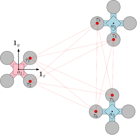
Figure 1: Problem setup and notation used. Each agent possesses a reference point $a_{\alpha}$ where $\alpha$ is the agent ID, as well as two tags $\tau_{i},\tau_{j}$, where $i,j$ are the tag IDs. $\mbf{1}_{x}$ and $\mbf{1}_{y}$ are vectors which represent the $x$ and $y$ axis of Agent 1’s body frame. Throughout this paper, the red agent is the arbitrary reference agent, and it will always be Agent 1 without loss of generality.

II-A State Definition and Range Measurement Model

Since the agents are rigid bodies, an orthonormal reference frame attached to their bodies can be defined. A position vector representing the position of point $z$, relative to point $w$, resolved in the body frame of agent $\alpha$ is denoted $\mbf{r}^{zw}_{\alpha}\in\mathbb{R}^{n}$. The attitude of the body frame on agent $\alpha$ relative to the body frame on agent $\beta$ is represented with a rotation matrix $\mbf{C}_{\alpha\beta}\in SO(n)$ such that $\mbf{r}^{zw}_{\alpha}=\mbf{C}_{\alpha\beta}\mbf{r}^{zw}_{\beta}$. The relative position and attitude between agents $\alpha$ and $\beta$, $(\mbf{r}^{a_{\beta}a_{\alpha}}_{\alpha},\mbf{C}_{\alpha\beta})$ define the relative pose between them, and can be packaged together in a pose transformation matrix

$$\mbf{T}_{\alpha\beta}=\left[\begin{array}[]{ cc}\mbf{C}_{\alpha\beta}&\mbf{r}^{a_{\beta}a_{\alpha}}_{\alpha}\\ \mbf{0}&1\end{array}\right]\in SE(n).$$ (1)

The exponential and logarithmic maps of the special Euclidean group $SE(n)$ are denoted $\exp:\mathfrak{se}(n)\to SE(n)$ and $\ln:SE(n)\to\mathfrak{se}(n)$, respectively, where $\mathfrak{se}(n)$ is the Lie algebra of $SE(n)$. The common “wedge” operator $(\cdot)^{\wedge}:\mathbb{R}^{m}\to\mathfrak{se}(n)$ and “vee” operator $(\cdot)^{\vee}:\mathfrak{se}(n)\to\mathbb{R}^{m}$ are also used in this paper. For a more thorough background on matrix Lie groups, including expressions for the aforementionned operators, see [21, 22].

Throughout this paper, Agent 1 will be the arbitary reference agent, such that the poses of all the other agents are expressed relative to Agent 1

$$\mbf{x}=(\mbf{T}_{12},\ldots,\mbf{T}_{1N}).$$ (2)

A single generic range measurement between tag $i$ and tag $j$ is modelled as a function of the state $\mbf{x}=(\mbf{T}_{12},\ldots,\mbf{T}_{1N})$ with

$$y_{ij}(\mbf{x}) =||\mbf{C}_{1\alpha}\mbf{r}^{\tau_{i}a_{\alpha}}_{\alpha}+\mbf{r}^{a_{\alpha}a_{1}}_{1}-(\mbf{C}_{1\beta}\mbf{r}^{\tau_{j}a_{\beta}}_{\beta}+\mbf{r}^{a_{\beta}a_{1}}_{1})||+v_{ij},$$ (3)

where $\alpha=\ell(i),$ $\beta=\ell(j)$, and $v_{ij}\sim\mathcal{N}(0,\sigma^{2}_{ij})$. This can be written compactly with the pose transformation matrices,

$$y_{ij}(\mbf{x}) =\left\|\mbf{D}\mbf{T}_{1\alpha}\left[\begin{array}[]{ c}\mbf{r}^{\tau_{i}a_{\alpha}}_{\alpha}\\ 1\end{array}\right]-\mbf{D}\mbf{T}_{1\beta}\left[\begin{array}[]{ c}\mbf{r}^{\tau_{j}a_{\beta}}_{\beta}\\ 1\end{array}\right]\right\|+v_{ij}$$ (8)

$$\triangleq\left\|\mbf{D}\mbf{T}_{1\alpha}\mbf{p}_{i}-\mbf{D}\mbf{T}_{1\beta}\mbf{p}_{j}\right\|+v_{ij},$$ (9)

where $\mbf{D}=[\mbf{1}\;\mbf{0}]$. In fact, the state $\mbf{x}=(\mbf{T}_{12},\ldots,\mbf{T}_{1N})$, written here as a tuple of pose matrices, is an element of a Lie group of its own,

$$\mbf{x}\in SE(n)\times\ldots\times SE(n)\triangleq SE(n)^{N-1}.$$

The group operation for $SE(n)^{N-1}$ is the elementwise matrix multiplication of the pose matrices in two arbitrary tuples, and the group inverse is the elementwise matrix inversion of the elements of the tuple $\mbf{x}$. The $\oplus$ operator is defined here as

$$\mbf{x}\oplus\delta\mbf{x}=\left(\mbf{T}_{12}\exp(\delta{\boldsymbol{\xi}}_{2}^{\wedge}),\;\ldots\;,\mbf{T}_{1N}\exp(\delta{\boldsymbol{\xi}}_{N}^{\wedge})\right),$$ (10)

where $\delta{\boldsymbol{\xi}}_{i}\in\mathbb{R}^{m}$, $\delta\mbf{x}=[\delta{\boldsymbol{\xi}}_{2}^{\mathsf{T}}\;\ldots\;\delta{\boldsymbol{\xi}}_{N}^{\mathsf{T}}]^{\mathsf{T}}\in\mathbb{R}^{m(N-1)}$, and will be used throughout the paper.

III Optimization

The goal is to find the relative agent poses that, with respect to some metric, provide the best relative pose estimation results if the estimation were to be done exclusively using the range measurements. The metric chosen in this paper is based on Fischer information and the Cramér-Rao bound, which will be recalled here.

Definition 1 (Fischer information matrix [23])

Let $\mbf{y}\in\mathbb{R}^{q}$ be a continuous random variable that is conditioned on a nonrandom variable $\mbf{x}\in\mathbb{R}^{n}$. The Fischer information matrix (FIM) is defined as

$$\mbf{I}(\mbf{x})=\mathbb{E}\left[\left(\frac{\partial\ln p(\mbf{y}|\mbf{x})}{\partial\mbf{x}}\right)^{\mathsf{T}}\left(\frac{\partial\ln p(\mbf{y}|\mbf{x})}{\partial\mbf{x}}\right)\right]\in\mathbb{R}^{n\times n},$$ (11)

where $\mathbb{E}[\cdot]$ is the expectation operator and $p(\cdot)$ denotes a probability density function.

Theorem 1 (Cramér-Rao Bound [23])

Let $\mbf{y}\in\mathbb{R}^{q}$ be a continuous random variable that is conditioned on $\mbf{x}\in\mathbb{R}^{n}$. Let ${\hat{\mbf{x}}}(\mbf{y})$ be an unbiased estimator of $\mbf{x}$, i.e., $\mathbb{E}[\mbf{e}(\mbf{x})]=\mathbb{E}[{\hat{\mbf{x}}}(\mbf{y})-\mbf{x}]=\mbf{0}$. The Cramér-Rao lower bound states that

$$\mathbb{E}\left[\mbf{e}(\mbf{x})\mbf{e}(\mbf{x})^{\mathsf{T}}\right]\geq\mbf{I}^{-1}(\mbf{x}).$$ (12)

Theorem 2 (FIM for a Gaussian PDF)

Consider the nonlinear measurement model with additive Gaussian noise,

$$\mbf{y}=\mbf{g}(\mbf{x})+\mbf{v},\qquad\mbf{v}\sim\mathcal{N}(\mbf{0},\mbf{R}).$$ (13)

The Fischer information matrix is given by

$$\mbf{I}(\mbf{x})=\mbf{H}(\mbf{x})^{\mathsf{T}}\mbf{R}^{-1}\mbf{H}(\mbf{x}),$$ (14)

where $\mbf{H}(\mbf{x})=\partial\mbf{g}(\mbf{x})/\partial\mbf{x}$.

The Cramér-Rao bound represents the minimum variance achievable by any unbiased estimator. Hence, motivated by Theorem 12, an estimation cost function $J_{\mathrm{est}}$ is defined

$$J_{\mathrm{est}}(\mbf{x})=-\ln\det\mbf{I}(\mbf{x}),$$ (15)

which will be minimized with the agent relative poses $\mbf{x}$ as the optimization variables. The logarithm of the determinant of $\mbf{I}(\mbf{x})$ is one option amongst many choices of matrix norms, such as the trace or Frobenius norm. We have found the chosen cost function to behave well in terms of numerical optimization and, most importantly, goes to infinity when the FIM becomes non-invertible. The state $\mbf{x}$ is locally observable from measurements $\mbf{y}$ if the measurement Jacobian $\mbf{H}(\mbf{x})$ is full column rank, which also makes the FIM full rank. As will be seen in Section III-B, non-invertibility of the FIM also corresponds to formations that result in unobservable relative poses, which should be avoided.

To create a measurement model in the form of (13), the range measurements are all concatenated into a single vector

$$\mbf{y}(\mbf{x})=\underbrace{[\ldots\\ y_{ij}(\mbf{x})\\ \ldots]^{\mathsf{T}}}_{\triangleq\mbf{g}(\mbf{x})}+\mbf{v},\quad\forall(i,j)\in\mathcal{E},\;\mbf{v}\sim\mathcal{N}(\mbf{0},\mbf{R}),$$

where $\mbf{R}=\mathrm{diag}(\ldots,\sigma^{2}_{ij},\ldots)$. It would be possible to directly descend the cost in (15) with an optimization algorithm such as gradient descent, if not for the fact that the state $\mbf{x}$ does not belong to Euclidean space $\mathbb{R}^{n}$ but rather $SE(n)^{N-1}$. As such, the expression $\partial\mbf{g}(\mbf{x})/\partial\mbf{x}$ is meaningless unless properly defined.

III-A On-manifold Cost and Gradient Descent

The modification employed in this paper is to reparameterize the measurement model by defining $\mbf{x}={\bar{\mbf{x}}}\oplus\delta\mbf{x}$, leading to

$$\mbf{y}=\mbf{g}({\bar{\mbf{x}}}\oplus\delta\mbf{x})+\mbf{v}\triangleq{\bar{\mbf{g}}}(\delta\mbf{x}).$$ (16)

The state ${\bar{\mbf{x}}}$ will represent the current optimization iterate, which will be updated using $\delta\mbf{x}$.

Since the argument of the new measurement model ${\bar{\mbf{g}}}(\delta\mbf{x})$ now belongs to Euclidean space $\mathbb{R}^{m(N-1)}$, it is possible to compute the “local” approximation to the FIM [24] at $\mbf{x}={\bar{\mbf{x}}}$ with $\mbf{I}({\bar{\mbf{x}}})=\mbf{H}({\bar{\mbf{x}}})^{\mathsf{T}}\mbf{R}^{-1}\mbf{H}({\bar{\mbf{x}}})$ where

$$\mbf{H}({\bar{\mbf{x}}})=\left.\frac{\partial\mbf{g}({\bar{\mbf{x}}}\oplus\delta\mbf{x})}{\partial\delta\mbf{x}}\right|_{\delta\mbf{x}=\mbf{0}},$$

and evaluate the cost function $J_{\mathrm{est}}({\bar{\mbf{x}}})=-\ln\det\mbf{I}({\bar{\mbf{x}}})$. Finally, an on-manifold gradient descent step can be taken with

$${\bar{\mbf{x}}}\leftarrow{\bar{\mbf{x}}}\oplus\left(-\gamma\left.\frac{\partial J_{\mathrm{est}}({\bar{\mbf{x}}}\oplus\delta\mbf{x})}{\partial\delta\mbf{x}}\right|_{\delta\mbf{x}=\mbf{0}}\right)^{\mathsf{T}},$$ (17)

where $\gamma$ is a step size.

The proposed gradient descent procedure is actually a standard approach to optimization on matrix manifolds [25]. From a differential-geometric point of view, an approximation to the FIM is computed in the tangent space of the current optimization iterate ${\bar{\mbf{x}}}$, which is a familiar Euclidean vector space. A gradient descent step is computed in the tangent space, and the result is retracted back to the manifold $SE(n)^{N-1}$ using the retraction $\mathcal{R}_{{\bar{\mbf{x}}}}(\delta\mbf{x})={\bar{\mbf{x}}}\oplus\delta\mbf{x}$.

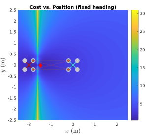
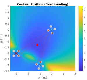
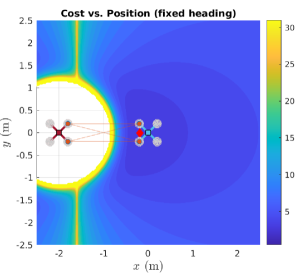
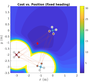
Figure 2: All four plots show the value of the cost with varying agent position (right agent for two-agent scenario, top agent for three-agent scenario), while maintaining fixed heading. The top row shows only the estmation cost $J_{\mathrm{est}}$, while the bottom row shows the total cost $J$ including the collision avoidance term.

III-B Cost function implementation

Creating an implementable expression for the cost function $J_{\mathrm{est}}({\bar{\mbf{x}}})=-\ln\det\left(\mbf{H}({\bar{\mbf{x}}})^{\mathsf{T}}\mbf{R}^{-1}\mbf{H}({\bar{\mbf{x}}})\right)$ eventually amounts to computing the Jacobian of the range measurement model (9) with respect to $\delta{\boldsymbol{\xi}}_{\alpha}$ and $\delta{\boldsymbol{\xi}}_{\beta}$. To see this,

$$\mbf{H}({\bar{\mbf{x}}})=\left[\begin{array}[]{ c}\vdots\\ \mbf{H}^{ij}({\bar{\mbf{x}}})\\ \vdots\end{array}\right],$$

$$\mbf{H}^{ij}({\bar{\mbf{x}}})=[\mbf{0}\ldots\mbf{H}^{ij}_{\alpha}({\bar{\mbf{x}}})\ldots\mbf{H}^{ij}_{\beta}({\bar{\mbf{x}}})\ldots\mbf{0}],$$

where

$$\mbf{H}^{ij}_{\alpha}({\bar{\mbf{x}}}) \triangleq\left.\frac{\partial y_{ij}({\bar{\mbf{x}}}\oplus\delta\mbf{x})}{\partial\delta{\boldsymbol{\xi}}_{\alpha}}\right|_{\delta\mbf{x}=\mbf{0}},$$

$$\mbf{H}^{ij}_{\beta}({\bar{\mbf{x}}}) \triangleq\left.\frac{\partial y_{ij}({\bar{\mbf{x}}}\oplus\delta\mbf{x})}{\partial\delta{\boldsymbol{\xi}}_{\beta}}\right|_{\delta\mbf{x}=\mbf{0}}.$$

The row matrix $\mbf{H}^{ij}({\bar{\mbf{x}}})\in\mathbb{R}^{1\times m(N-1)}$ represents the Jacobian of a single range measurement $y_{ij}$ with respect to the full state perturbation $\delta\mbf{x}$. This resulting matrix will be zero everywhere except for two blocks $\mbf{H}^{ij}_{\alpha}({\bar{\mbf{x}}})\in\mathbb{R}^{1\times m}$ and $\mbf{H}^{ij}_{\beta}({\bar{\mbf{x}}})\in\mathbb{R}^{1\times m}$, respectively located at the $\alpha^{\textrm{th}}$ and $\beta^{\textrm{th}}$ block columns, and have closed-form expressions derived in Appendix -A.

The cost function $J_{\mathrm{est}}$ is visualized for varying agent position in the top row of Figure 2, where the red dot shows the minimum found within that view. Looking at the top-left plot of Figure 2, there is a vertical line of high cost near the agent on the left, corresponding exactly to when all four tags line up, leading to an unobservable formation. Similarly, the three-agent scenario in the top-right plot of Figure 2 shows a high cost when the agents are nearly all on the same line, which is a situation of near-unobservability. However, as can be seen in the top-left plot, the minimum is unacceptably close to the left agent, which would cause them to collide. Indeed, we have observed that naively descending the cost $J_{\mathrm{est}}$ alone leads to all the agents collapsing into each other. An explanation for this behavior is that when agents are closer together, changes in attitude result in larger changes in the range measurements, which increases Fischer information. Nevertheless, in practice, collisions must be avoided, and this is done by augmenting the cost with an additional collision avoidance term $J_{\mathrm{col}}(\mbf{x})$, such that the total cost $J(\mbf{x})$ is

$$J(\mbf{x})=J_{\mathrm{est}}(\mbf{x})+J_{\mathrm{col}}(\mbf{x}),\qquad J_{\mathrm{col}}(\mbf{x})=\sum_{\begin{subarray}{c}\alpha,\beta\in\mathcal{A}\\ \alpha\neq\beta\end{subarray}}J_{\mathrm{col}}^{\alpha\beta}(\mbf{x}),$$

where a collision avoidance cost from [26] is used,

$$J_{\mathrm{col}}^{\alpha\beta}(\mbf{x})=\left(\min\left\{0,\frac{\left\|\mbf{r}^{a_{\alpha}a_{\beta}}_{1}\right\|^{2}-R^{2}}{\left\|\mbf{r}^{a_{\alpha}a_{\beta}}_{1}\right\|^{2}-d^{2}}\right\}\right)^{2}.$$ (18)

The term $R$ represents an “activation radius” and $d$ is the safety collision avoidance radius. In this paper, the agent relative position is expressed as a function of pose matrices with

$$\mbf{r}^{a_{\alpha}a_{\beta}}_{1}=\mbf{D}\mbf{T}_{1\alpha}\mbf{b}-\mbf{D}\mbf{T}_{1\beta}\mbf{b},$$

where $\mbf{D}=[\mbf{1}\;\mbf{0}],$ $\mbf{b}=[\mbf{0}\;1]^{\mathsf{T}}$. The new cost function $J$ is plotted on the bottom row of Figure 2, showing the effect of the collision avoidance term. Finally, one is now ready to descend the cost directly with

$${\bar{\mbf{x}}}\leftarrow{\bar{\mbf{x}}}\oplus\left(-\gamma\left.\frac{\partial J({\bar{\mbf{x}}}\oplus\delta\mbf{x})}{\partial\delta\mbf{x}}\right|_{\delta\mbf{x}=\mbf{0}}\right)^{\mathsf{T}}.$$ (19)

In this work, the Jacobian of $J_{\mathrm{est}}$ is computed numerically with finite difference [27], and the optimization is only done offline for the following reasons. The solution to the optimization problem is only a function of some physical properties, the measurement graph $\mathcal{G}$, and the number of robots $N$. For any experiments that use the same hardware, the physical properties such as the safety radius, tag locations, and measurement covariances, all remain constant. The measurement graph $\mathcal{G}$ can often also be assumed to be constant and fully connected. Even though full-connectedness is not necessary to find optimal formations using the proposed approach, technologies such as UWB often have a ranging limit that is well beyond the true ranges between all robots in the experiment. Hence, it is straightforward to precompute optimal formations for varying robot numbers $N$ with fully-connected measurement graphs, and to store the solutions in memory onboard each robot.

Nevertheless, a distributed, real-time implementation is required for varying measurement graphs, which is likely to arise in the presence of obstacles that block line-of-sight. Such a scenario requires simultaneously satisfying obstacle avoidance constraints and perhaps other planning objectives, which is beyond the scope of this paper.

III-C Optimization results

The gradient descent in (19) is performed with a step size of $\gamma=0.1$, an activation radius of $R=2~{}\mathrm{m}$, and a safety radius of $d=1~{}\mathrm{m}$. Each agent has two tags located at

$$\mbf{r}^{\tau_{i}a_{\alpha}}_{\alpha}=[0.2\;0.2]^{\mathsf{T}},\quad\text{and}\quad\mbf{r}^{\tau_{j}a_{\alpha}}_{\alpha}=[0.2\;-0.2]^{\mathsf{T}},$$

where $\alpha,i,j$ are arbitrary and the units are in meters. Figure 3 shows quadcopter formations at convergence for 3, 4, 5, and 10 agents, each with a fully-connected measurement graph $\mathcal{G}$, except for edges corresponding to two tags on the same agent. The results shown here are intuitive, with the three- and four-agent scenarios corresponding to an equilateral triangle and square, respectively. However, with increasing agent numbers, regular polygon formations are no longer optimal, as can be seen in the five- and ten-agent scenarios.

Since the treatment in this paper is general to an arbitary measurement graph $\mathcal{G}$, provided the FIM remains maximum rank, optimization is also performed for a non-fully-connected measurement graph. The results for this along with a 3D scenario are shown in Figure 4. In 3D, the robot relative poses are represented with elements of $SE(3)$. However, since the presented simulations contain only two-tag robots, relative roll and pitch between robots are unobservable, which would make the cost infinite, unless more sensors are used. Hence, roll and pitch are excluded from the optimization and their values are fixed to zero. This leaves the three translational components and heading as the four degrees of freedom available for optimization. This is easily implemented in practice with a redefinition of the “wedge” operator such that $(\cdot)^{\wedge}:\mathbb{R}^{4}\to\mathfrak{se}(3)$. Moreover, from an application standpoint, both ground vehicles and quadcopter-type aerial vehicles only have heading as a rotational degree of freedom available for planning.

III-D Validation on a least squares estimator

To validate the claim that descending the cost improves the estimation performance, a non-linear least-squares estimator is used. At regular iterates ${\bar{\mbf{x}}}$ of the optimization trajectory, a small 2000-trial Monte Carlo experiment is performed, where in each trial a set of range measurements are generated with $\mbf{y}=\mbf{g}({\bar{\mbf{x}}})+\mbf{v},$ $\mbf{v}=\mathcal{N}(\mbf{0},\mbf{R})$. Then, an on-manifold Gauss-Newton procedure [22] is used to solve

$${\hat{\mbf{x}}}=\arg\min_{\mbf{x}}\frac{1}{2}\sum_{\alpha=2}^{N}\left\|\ln(\mbf{C}_{1\alpha}^{\mathsf{T}}{\check{\mbf{C}}}_{1\alpha})^{\vee}\right\|^{2}_{{\check{\mbf{P}}}_{\alpha}}+\frac{1}{2}\left\|\mbf{y}-\mbf{g}(\mbf{x})\right\|^{2}_{\mbf{R}},$$ (20)

where $\left\|\mbf{e}\right\|{M}^{2}=\mbf{e}^{\mathsf{T}}\mbf{M}^{-1}\mbf{e}$ denotes a squared Mahalanobis distance, and an attitude prior with “mean” ${\check{\mbf{C}}}_{1\alpha}$ and covariance ${\check{\mbf{P}}}_{\alpha}$ is also included for each agent. It turns out that minimization of only the second term in (20) yields unacceptably poor estimation performance, as the solution often converges to local minimums depending on the initial guess. The inclusion of an attitude prior, which is practically obtained by dead-reckoning on-board gyroscope measurements, yields much lower overall estimation error.

Figure 6 shows the value of the cost throughout the optimization trajectory, as well as the mean squared estimation error over the $K=2000$ Monte Carlo trials per optimization step. The true agent poses are initialized in a near-straight line, as shown in Figure 5, and the covariances used are $\mbf{R}=0.1^{2}\mbf{1}~{}\mathrm{m}^{2}$, ${\check{\mbf{P}}}_{\alpha}=0.08^{2}~{}\mathrm{rad}^{2}$. The mean squared estimation error (MSE) is calculated with

$$\mathrm{MSE}=\frac{1}{K}\sum_{k=1}^{K}\delta{\boldsymbol{\xi}}^{\mathsf{T}}\delta{\boldsymbol{\xi}},\qquad\delta{\boldsymbol{\xi}}=\left[\begin{array}[]{ c}\ln({\bar{\mbf{T}}}_{12}^{-1}{\hat{\mbf{T}}}_{12})^{\vee}\\ \vdots\\ \ln({\bar{\mbf{T}}}_{1N}^{-1}{\hat{\mbf{T}}}_{1N})^{\vee}\end{array}\right],$$ (21)

and shows a clear correlation with the cost function. This provides evidence for the fact that descending the proposed cost function also reduces the estimation error.

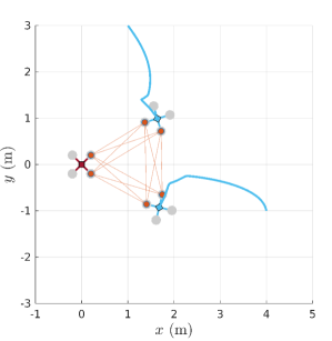
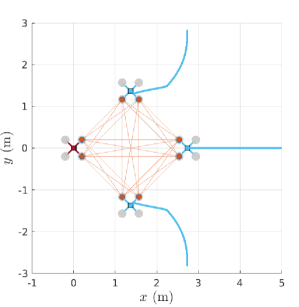
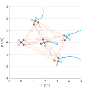
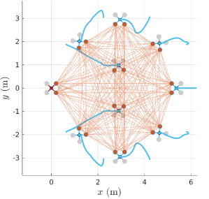
Figure 3: Final locally optimal formations for 3, 4, 5, and 10 agents.

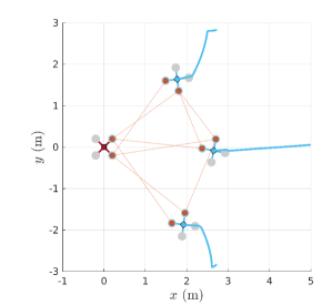
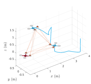
Figure 4: (left) Optimal formation with sparse measurement graph. (right) Optimal formation with 3D position and heading as design variables.

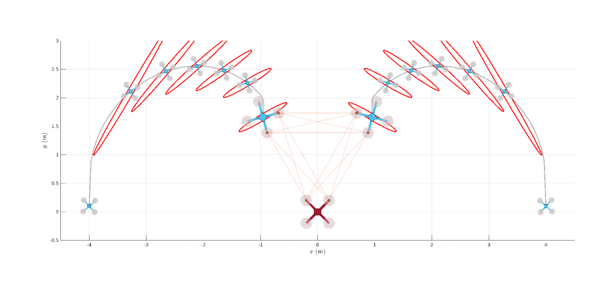
Figure 5: Trajectory taken during optimization with superimposed $1\sigma$ equal-probability contours corresponding to the Cramér-Rao bound. The ellipsoids for the starting positions are too large to fit in the figure.

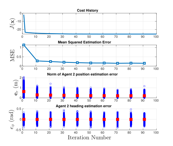
Figure 6: Cost function, along with various metrics of a least-squares estimator, obtained from 2000 Monte-Carlo trials at various points during the optimization. In the bottom two plots, the red squares denote the average norm of the respective estimation errors.

IV Experimental Evaluation

An estimator is also run with three PX4-based Uvify IFO-S quadcopters in order to experimentally validate the claim that descending the proposed cost function results in improved estimation performance. The quadcopters start by flying in a line formation and, after 30 seconds, proceed to a triangle formation computed using the proposed framework for another 30 seconds, as shown in Figure 8. Figure 7 shows the position estimation error using the least-squares estimator presented in Section III-D. Real gyroscope measurements are used to obtain an attitude prior at all times. Range measurements are synthesized with a standard deviation of 10 cm using ground truth vehicle poses obtained from a motion capture system. The UWB tags are simulated to be 17 cm apart, corresponding to extremities of the propeller arms. As can be seen in Figure 7, moving to the optimal triangle formation, from one of the worst starting formations results in a 68% reduction in estimation variance.

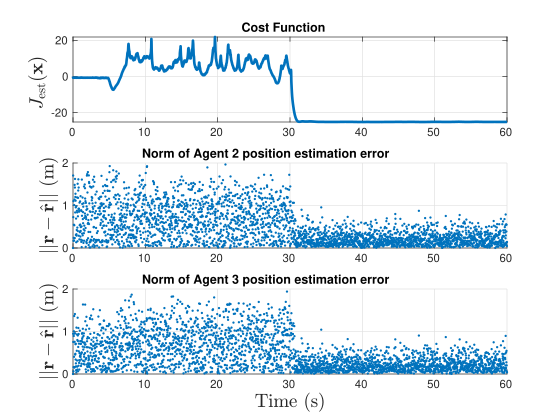
Figure 7: Experimental results using a least squares estimator. From 0 s to 30 s, the quadcopters are in a line formation and the average positioning error is 0.77 m. From 30 s to 60 s, the quadcopters are in an optimal formation and the average positioning error is 0.22 m, a 68% reduction.

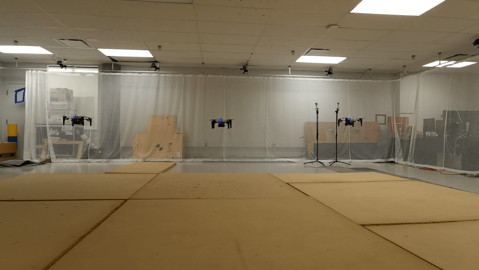
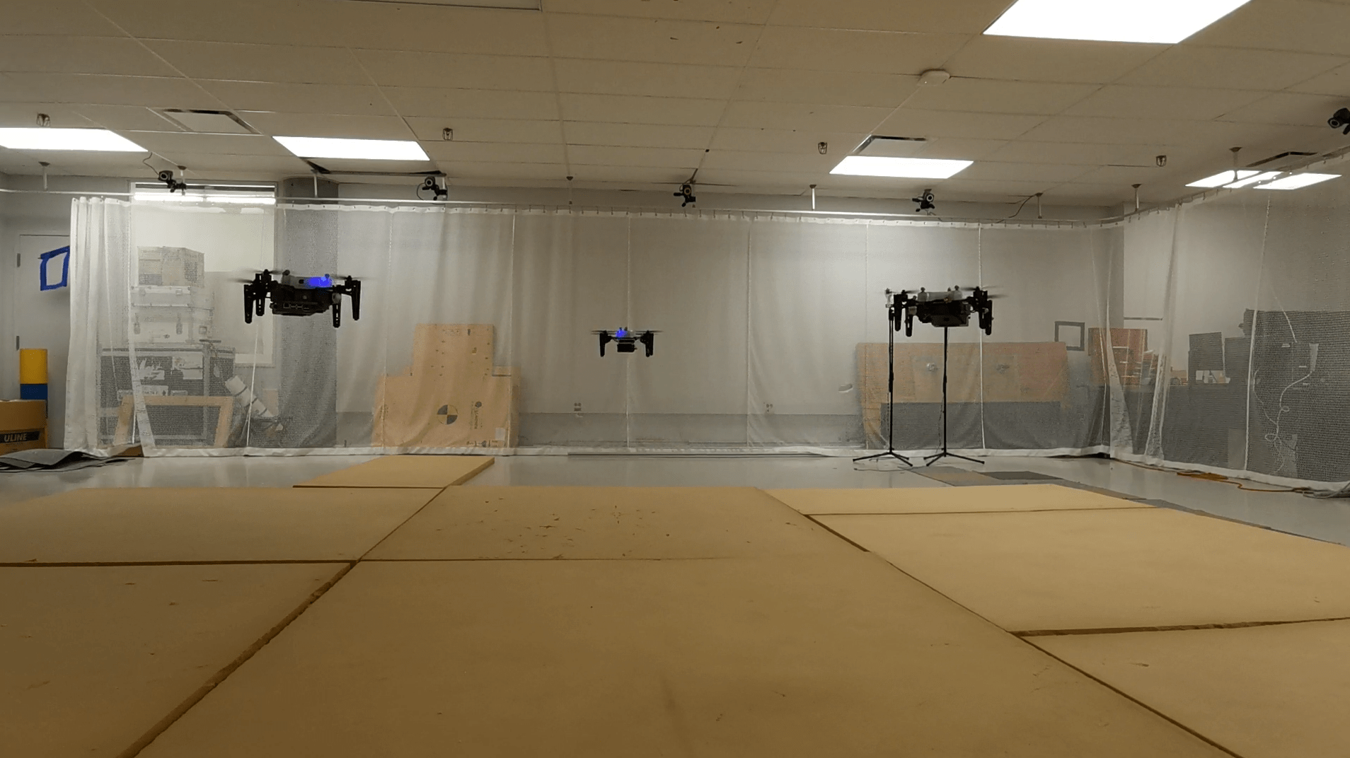
Figure 8: (top) Three quadcopters in an initial straight line formation. (bottom) Quadcopters in an optimal triangle formation.

V Conclusion

This paper shows, in both simulation and experiment, that range-based relative state estimation performance can be substantially improved by a proper choice of formation geometry. The largest improvements are obtained when the robots move away from unobservable formations.

The generalizability of the cost function makes it appropriate for use beyond direct minimization. For instance, consider using this function to impose an inequality constraint on an application-oriented planning problem, such as indoor exploration. Using an inequality constraint would allow robots the freedom to move within the feasible region in order to accomplish tasks such as infrastructure inspection, yet still avoid the “worst” formations with very high cost, which could cause problematically large state estimation errors. Future work may tackle a scenario similar to this, including developing a distributed computation scheme for the proposed cost function.

-A Measurement model Jacobian

Let $y_{ij}(\mbf{x})=y_{ij}({\bar{\mbf{x}}})+\delta y_{ij}\triangleq\bar{y}_{ij}+\delta y_{ij}$, $\mbf{T}_{1\alpha}={\bar{\mbf{T}}}_{1\alpha}\exp(\delta{\boldsymbol{\xi}}_{\alpha}^{\wedge})$, $\mbf{T}_{1\beta}={\bar{\mbf{T}}}_{1\beta}\exp(\delta{\boldsymbol{\xi}}_{\beta}^{\wedge})$, and $v_{ij}=0$. The terms $\delta y_{ij},\delta{\boldsymbol{\xi}}_{\alpha},\delta{\boldsymbol{\xi}}_{\beta}$ are assumed to be small quantities, which motivates, for example, the approximation $\exp(\delta{\boldsymbol{\xi}}_{\alpha}^{\wedge})\approx\mbf{1}+\delta{\boldsymbol{\xi}}_{\alpha}^{\wedge}$. Equation (9) becomes

$$(\bar{y}_{ij}+\delta y_{ij})^{2}=\left(\mbf{D}{\bar{\mbf{T}}}_{1\alpha}(\mbf{1}+\delta{\boldsymbol{\xi}}_{\alpha}^{\wedge})\mbf{p}_{i}-\mbf{D}{\bar{\mbf{T}}}_{1\beta}(\mbf{1}+\delta{\boldsymbol{\xi}}_{\beta}^{\wedge})\mbf{p}_{j}\right)^{\mathsf{T}}\\ \left(\mbf{D}{\bar{\mbf{T}}}_{1\alpha}(\mbf{1}+\delta{\boldsymbol{\xi}}_{\alpha}^{\wedge})\mbf{p}_{i}-\mbf{D}{\bar{\mbf{T}}}_{1\beta}(\mbf{1}+\delta{\boldsymbol{\xi}}_{\beta}^{\wedge})\mbf{p}_{j}\right),$$

which, after expanding and neglecting higher-order terms, leads to

$$2\bar{y}_{ij}\delta y_{ij}=2(\mbf{p}_{i}^{\mathsf{T}}{\bar{\mbf{T}}}_{1\alpha}^{\mathsf{T}}\mbf{D}^{\mathsf{T}}-\mbf{p}_{j}^{\mathsf{T}}{\bar{\mbf{T}}}_{1\beta}^{\mathsf{T}}\mbf{D}^{\mathsf{T}})\mbf{D}{\bar{\mbf{T}}}_{1\alpha}\delta{\boldsymbol{\xi}}^{\wedge}_{\alpha}\mbf{p}_{i}\\ +2(\mbf{p}_{j}^{\mathsf{T}}{\bar{\mbf{T}}}_{1\beta}^{\mathsf{T}}\mbf{D}^{\mathsf{T}}-\mbf{p}_{i}^{\mathsf{T}}{\bar{\mbf{T}}}_{1\alpha}^{\mathsf{T}}\mbf{D}^{\mathsf{T}})\mbf{D}{\bar{\mbf{T}}}_{1\beta}\delta{\boldsymbol{\xi}}^{\wedge}_{\beta}\mbf{p}_{i}.$$ (22)

Next, it is straightforward to define a simple operator $(\cdot)^{\odot}$, as per [22], such that ${\boldsymbol{\xi}}^{\wedge}\mbf{p}=\mbf{p}^{\odot}{\boldsymbol{\xi}}$. Rearranging (22) yields

$$\delta y_{ij}=\frac{(\mbf{p}_{i}^{\mathsf{T}}{\bar{\mbf{T}}}_{1\alpha}^{\mathsf{T}}\mbf{D}^{\mathsf{T}}-\mbf{p}_{j}^{\mathsf{T}}{\bar{\mbf{T}}}_{1\beta}^{\mathsf{T}}\mbf{D}^{\mathsf{T}})}{\bar{y}_{ij}}\mbf{D}{\bar{\mbf{T}}}_{1\alpha}\mbf{p}_{i}^{\odot}\delta{\boldsymbol{\xi}}_{\alpha}\\ -\underbrace{\frac{(\mbf{p}_{i}^{\mathsf{T}}{\bar{\mbf{T}}}_{1\alpha}^{\mathsf{T}}\mbf{D}^{\mathsf{T}}-\mbf{p}_{j}^{\mathsf{T}}{\bar{\mbf{T}}}_{1\beta}^{\mathsf{T}}\mbf{D}^{\mathsf{T}})}{\bar{y}_{ij}}}_{\triangleq{\boldsymbol{\rho}}_{ij}}\mbf{D}{\bar{\mbf{T}}}_{1\beta}\mbf{p}_{j}^{\odot}\delta{\boldsymbol{\xi}}_{\beta}.$$ (23)

The term ${\boldsymbol{\rho}}_{ij}$ is the physical unit direction vector between tags $i$ and $j$, resolved in Agent 1’s body frame. From (23) it then follows that

$$\frac{\partial y_{ij}}{\partial\delta{\boldsymbol{\xi}}_{\alpha}}={\boldsymbol{\rho}}_{ij}\mbf{D}{\bar{\mbf{T}}}_{1\alpha}\mbf{p}_{i}^{\odot},\qquad\frac{\partial y_{ij}}{\partial\delta{\boldsymbol{\xi}}_{\beta}}=-{\boldsymbol{\rho}}_{ij}\mbf{D}{\bar{\mbf{T}}}_{1\beta}\mbf{p}_{j}^{\odot}.$$

References

- [1] Shushuai Li, Christophe De Wagter and Guido C. H. E. Croon “Self-supervised Monocular Multi-robot Relative Localization with Efficient Deep Neural Networks”, 2021 arXiv: http://arxiv.org/abs/2105.12797
- [2] Ling Mao, Jiapin Chen, Zhenbo Li and Dawei Zhang “Relative Localization Method of Multiple Micro Robots Based on Simple Sensors” In Intl. J. of Adv. Robotic Sys. 10, 2013, pp. 1–9 DOI: 10.5772/55587
- [3] Zafer Sahinoglu, Sinan Gezici and Ismail Guvenc “Ultra-wideband Positioning Systems” New York, NY: Cambridge University Press, 2008
- [4] Samet Guler, Mohamed Abdelkader and Jeff S. Shamma “Infrastructure-free Localization of Aerial Robots with Ultrawideband Sensors” In American Control Conference, 2019, pp. 13–18 arXiv:1809.08218
- [5] Thien Minh Nguyen et al. “Robust Target-Relative Localization with Ultra-Wideband Ranging and Communication” In IEEE Intl. Conf. on Robotics and Automation, 2018, pp. 2312–2319 DOI: 10.1109/ICRA.2018.8460844
- [6] Kexin Guo, Xiuxian Li and Lihua Xie “Ultra-wideband and odometry-based cooperative relative localization with application to multi-UAV formation control” In IEEE Trans. on Cybernetics 50.6 IEEE, 2020, pp. 2590–2603 DOI: 10.1109/TCYB.2019.2905570
- [7] Thien Minh Nguyen et al. “Distance-Based Cooperative Relative Localization for Leader-Following Control of MAVs” In IEEE Robotics and Automation Letters 4.4 IEEE, 2019, pp. 3641–3648 DOI: 10.1109/LRA.2019.2926671
- [8] Thien Minh Nguyen et al. “Persistently Excited Adaptive Relative Localization and Time-Varying Formation of Robot Swarms” In IEEE Trans. on Robotics 36.2 IEEE, 2020, pp. 553–560 DOI: 10.1109/TRO.2019.2954677
- [9] Charles Champagne Cossette et al. “Relative Position Estimation between Two UWB Devices with IMUs” In IEEE Robotics and Automation Letters 6.3 Institute of ElectricalElectronics Engineers Inc., 2021, pp. 4313–4320 DOI: 10.1109/LRA.2021.3067640
- [10] Thien Hoang Nguyen and Lihua Xie “Relative Transformation Estimation Based on Fusion of Odometry and UWB Ranging Data”, 2022, pp. 1–15 arXiv: http://arxiv.org/abs/2202.00279
- [11] Pedro Batista, Carlos Silvestre and Paulo Oliveira “Single Range Aided Navigation and Source Localization: Observability and Filter design” In Systems and Control Letters 60.8 Elsevier B.V., 2011, pp. 665–673 DOI: 10.1016/j.sysconle.2011.05.004
- [12] Fujiang She et al. “Enhanced Relative Localization Based on Persistent Excitation for Multi-UAVs in GPS-Denied Environments” In IEEE Access 8, 2020, pp. 148136–148148 DOI: 10.1109/ACCESS.2020.3015593
- [13] Hao Xu et al. “Decentralized Visual-Inertial-UWB Fusion for Relative State Estimation of Aerial Swarm” In IEEE Intl. Conf. on Robotics and Automation, 2020, pp. 8776–8782 arXiv:2003.05138
- [14] Benjamin Hepp, Tobias Nägeli and Otmar Hilliges “Omni-directional Person Tracking on a Flying Robot using Occlusion-robust Ultra-wideband Signals” In IEEE Intl. Conf. on Intelligent Robots and Systems, 2016, pp. 189–194 DOI: 10.1109/IROS.2016.7759054
- [15] Mohammed Shalaby, Charles Champagne Cossette, James Richard Forbes and Jerome Le Ny “Relative Position Estimation in Multi-Agent Systems Using Attitude-Coupled Range Measurements” In IEEE Robotics and Automation Letters 6.3, 2021, pp. 4955–4961 DOI: 10.1109/LRA.2021.3067253
- [16] Manon Kok and Arno Solin “Scalable Magnetic Field SLAM in 3D Using Gaussian Process Maps” In Intl. Conf. on Information Fusion, 2018, pp. 1353–1360 DOI: 10.23919/ICIF.2018.8455789
- [17] Arno Solin et al. “Modeling and Interpolation of the Ambient Magnetic Field by Gaussian Processes” In IEEE Trans. on Robotics 34.4, 2018, pp. 1112–1127 DOI: 10.1109/TRO.2018.2830326
- [18] Wenda Zhao, Marijan Vukosavljev and Angela P. Schoellig “Optimal Geometry for Ultra-wideband Localization using Bayesian Optimization” In IFAC-PapersOnLine 53.2, 2020, pp. 15481–15488 DOI: 10.1016/j.ifacol.2020.12.2372
- [19] Jerome Le Ny and Simon Chauvière “Localizability-Constrained Deployment of Mobile Robotic Networks with Noisy Range Measurements” In American Control Conference, 2018, pp. 2788–2793
- [20] Justin Cano and Jerome Le Ny “Improving Ranging-Based Location Estimation with Rigidity-Constrained CRLB-Based Motion Planning” In Intl. Conf. on Robotics and Automation, 2021
- [21] Joan Solà, Jeremie Deray and Dinesh Atchuthan “A Micro Lie Theory for State Estimation in Robotics”, 2018, pp. 1–17 arXiv: http://arxiv.org/abs/1812.01537
- [22] Tim Barfoot “State Estimation for Robotics” Toronto, ON: Cambridge University Press, 2019
- [23] Yaakov Bar-Shalom, X.-Rong Li and Thiagalingam Kirubarajan “Estimation with Applications to Tracking and Navigation” New York: John Wiley & Sons, Inc., 2001
- [24] Silvère Bonnabel and Axel Barrau “An Intrinsic Cramér-Rao bound on Lie Groups” URL: https://arxiv.org/abs/1506.05662
- [25] P.A. Absil, R. Mahony and R. Sepulchre “Optimization Algorithms on Matrix Manifolds” Princeton Uni. Press, 2008
- [26] Yuanqing Xia, Xitai Na, Zhongqi Sun and Jing Chen “Formation Control and Collision Avoidance for Multi-Agent Systems Based on Position Estimation” In ISA Transactions 61.1, 2016, pp. 287–296
- [27] Charles Champagne Cossette, Alex Walsh and James Richard Forbes “The Complex-Step Derivative Approximation on Matrix Lie Groups” In IEEE Robotics and Automation Letters 5.2, 2020, pp. 906–913 DOI: 10.1109/LRA.2020.2965882