Dips at small sizes for topological obstruction sets

Abstract.

The Graph Minor Theorem of Robertson and Seymour implies a finite set of obstructions for any minor closed graph property. We observe that, for a wide range of topological properties, there is a dip in the obstruction set at small size. In particular, we show that there are only three obstructions to knotless embedding of size 23, which is far fewer than the 92 of size 22 and the hundreds known to exist at larger sizes. We also classify the 35 obstructions to knotless embedding of order 10.

1. Introduction

The Graph Minor Theorem of Robertson and Seymour [RS] implies that any minor closed graph property $\mathcal{P}$ is characterized by a finite set of obstructions. For example, planarity is determined by $K_{5}$ and $K_{3,3}$ [K, W] while linkless embeddability has seven obstructions, known as the Petersen family [RST]. However, Robertson and Seymour’s proof is highly non-constructive and it remains frustratingly difficult to identify the obstruction set, even for a simple property such as apex (see [JK]). Although we know that the obstruction set for a property $\mathcal{P}$ is finite, in practice it is often difficult to establish any useful bounds on its size.

In the absence of concrete bounds, information about the shape or distribution of an obstruction set would be welcome. Given that the number of obstructions is finite, one might anticipate a roughly normal distribution with a central maximum and numbers tailing off to either side. Indeed, many of the known obstruction sets do follow this pattern. In [MW, Table 2], the authors present a listing of more than 17 thousand obstructions for torus embeddings. Although, the list is likely incomplete, it does appear to follow a normal distribution both with respect to graph order and graph size, see Figure 1.

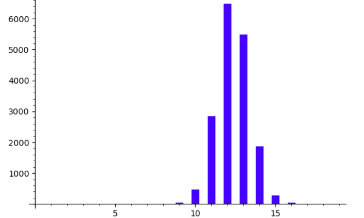
(a) By order

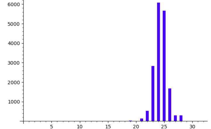
(b) By size

Figure 1. Distribution of torus embedding obstructions

Size	18	19	20	21	22	23	$\cdots$	28	29	30	31
Count	6	19	8	123	517	2821	$\cdots$	299	8	4	1

Table 1. Count of torus embedding obstructions by size.

However, closer inspection (see Table 1) shows that there is a dip, or local minimum, in the number of obstructions at size twenty. We will say that the dip occurs at small size meaning it is near the end of the left tail of the size distribution. Some properties in fact have a gap at small size, meaning there are sizes near the end of the left tail for which there are no obstructions at all. In the next section, we survey topological properties for which we know something about the obstruction set. Almost all exhibit a dip or gap at small size.

In Section 3, we prove the following.

Theorem 1.1.

There are exactly three obstructions to knotless embedding of size 23.

A knotless embedding of a graph is an embedding in $\mathbb{R}^{3}$ such that each cycle is a trivial knot. Since there are no obstructions of size 20 or less, 14 of size 21, 92 of size 22 and at least 156 of size 28 (see [FMMNN, GMN]), the theorem shows that the knotless embedding obstruction set also has a dip at small size, 23. In that section, we also pose a question: if $G$ has a vertex of degree less than three, is it true that no graph related to $G$ by a sequence of $\nabla\mathrm{Y}$ moves, nor any graph related to $G$ by a sequence of $\mathrm{Y}\nabla$ moves can be an obstruction for knotless embedding?

In Section 4, we prove the following.

Theorem 1.2.

There are exactly 35 obstructions to knotless embedding of order 10.

In contrast to graph size, distributions with respect to graph order generally do not have dips or gaps. In particular, Theorem 1.2 continues an increasing trend of no obstructions of order 6 or less, one obstruction of order 7 [CG], two of order 8 [CMOPRW, BBFFHL], and eight of order 9 [MMR].

2. Dips at small size

As mentioned in the introduction, it remains difficult to determine the obstruction set even for simple graph properties. In this section we survey the topological graph properties for which we know something about the obstruction set. Almost all demonstrate a gap or dip at small size. We will look at properties with a gap, a dip, and neither, in turn. Note that, as in Table 1, when we present data in a table, we begin with the extreme left end of the distribution. There are no obstructions of size smaller than that of the first column in our tables.

We begin with a listing of graph properties for which there is a gap at small size. The obstruction set for apex-outerplanar graphs was determined by Ding and Dziobiak [DD]. A graph is apex-outerplanar if it is outerplanar, or becomes outerplanar on deletion of a single vertex. The 57 obstructions are distributed by size as in Table 2. There are gaps at size 11, 16, and 17, and a dip at size 13. While this distribution has a gap at small size, 11, it is far from normal.

Size	9	10	11	12	13	14	15	16	17	18
Count	1	1	0	7	2	6	10	0	0	30

Table 2. Count of apex-outerplanar obstructions by size.

Various authors [JK, LMMPRTW, P] have investigated the set of apex obstructions. A graph is apex if it is planar, or becomes planar on deletion of a single vertex. As yet, we do not have a complete listing of the apex obstruction set, but Jobson and Kézdy [JK] report that there are at least 401 obstructions. Table 3 shows the classification of obstructions through size 21 obtained by Pierce [P] in his senior thesis. Note the gaps at size 16 and 17.

Size	15	16	17	18	19	20	21
Count	7	0	0	4	5	22	33

Table 3. Count of apex obstructions through size 21.

We say that a graph is 2-apex if it is apex, or becomes apex on deletion of a single vertex. Table 4 shows the little that we know about the obstruction set for this family [MP]. Aside from the counts for sizes 21 and 22 and the gap at size 23, we know only that there are obstructions for each size from 24 through 30.

Size	21	22	23
Count	20	60	0

Table 4. Count of 2-apex obstructions through size 23.

Most of the remaining topological properties whose obstruction set has been studied have a dip at small size. In the introduction, we mentioned the dip at size 20 for the torus obstructions. One of our main results, Theorem 1.1, demonstrates a dip at size 23 for knotless embedding. Table 5 shows the dip at size 17 for the 35 obstructions to embedding in the projective plane [A, GHW, MT].

Size	15	16	17	18	19	20
Count	4	8	7	12	2	2

Table 5. Count of projective planar obstructions by size.

A final example of a dip at small size is the 38 obstructions for outer-cylindrical graphs classified by Archdeacon et al. [ABDHS]. A graph is outer-cylindrical if it has a planar embedding so that all vertices fall on two faces. Table 6 illustrates the dip at size 11 for this obstruction set.

Size	9	10	11	12	13	14
Count	1	2	1	27	6	1

Table 6. Count of outer-cylindrical obstructions by size.

Some small obstruction sets have no gap or dip simply because they consist of only one or two sizes. There are two obstructions to planarity, one each of size 9 ($K_{3,3}$) and 10 ($K_{5}$). The two obstructions, $K_{4}$ and $K_{3,2}$, to outerplanarity both have size six and the seven obstructions to linkless embedding in the Petersen family [RST] are all of size 15. We know of only one example of a larger obstruction set for a topological property that exhibits no dip or gap. Archdeacon, Hartsfield, Little, and Mohar [AHLM] determined the 32 obstructions to outer-projective-planar embedding and Table 7 shows this set has no dips or gaps.

Size	10	11	12
Count	1	7	24

Table 7. Count of outer-projective-planar obstructions by size.

3. Knotless embedding obstructions of size 23

In this section we prove Theorem 1.1: there are exactly three obstructions to knotless embedding of size 23. In subsection 3.2 we ask a question that may be of independent interest. Question 3.7: If $\delta(G)<3$, is it true that $G$ has no MMIK descendants or ancestors? Definitions are given below.

We begin with some terminology. A graph that admits no knotless embedding is intrinsically knotted (IK). In contrast, we’ll call the graphs that admit a knotless embedding not intrinsically knotted (nIK). If $G$ is in the obstruction set for knotless embedding we’ll say $G$ is minor minimal intrinsically knotted (MMIK). This reflects that, while $G$ is IK, no proper minor of $G$ has that property. Similarly, we will call 2-apex obstructions minor minimal not 2-apex (MMN2A).

Our strategy for classifying MMIK graphs of size 23 is based on the following observation.

Lemma 3.1.

[BBFFHL, OT] If $G$ is 2-apex, then $G$ is not IK

Suppose $G$ is MMIK of size 23. By Lemma 3.1, $G$ is not 2-apex and, therefore, $G$ has an MMN2A minor. The MMN2A graphs through order 23 were classified in [MP]. All but eight of them are also MMIK and none are of size 23. It follows that a MMIK graph of size 23 has one of the eight exceptional MMN2A graphs as a minor. Our strategy is to construct all size 23 expansions of the eight exceptional graphs and determine which of those is in fact MMIK.

Before further describing our search, we remark that it does rely on computer support. Indeed, the initial classification of MMN2A graphs in [MP] is itself based on a computer search. We give a traditional proof that there are three size 23 MMIK graphs, which is stated as Theorem 3.2 below. We rely on computers only for the argument that there are no other size 23 MMIK graphs. We remark that even if we cannot provide a complete, traditional proof that there are no more than three size 23 MMIK graphs, our argument does strongly suggest that there are far fewer MMIK graphs of size 23 than the known 92 MMIK graphs of size 22 and at least 156 of size 28 [FMMNN, GMN]. In other words, even without computers, we have compelling evidence that there is a dip at size 23 for the obstructions to knotless embedding.

Below we give graph6 notation [Sg] and edge lists for the three MMIK graphs of size 23.

$G_{1}$ J@yaig[gv@?

$$[(0,4),(0,5),(0,9),(0,10),(1,4),(1,6),(1,7),(1,10),(2,3),(2,4),(2,5),(2,9),$$

$$(2,10),(3,6),(3,7),(3,8),(4,8),(5,6),(5,7),(5,8),(6,9),(7,9),(8,10)]$$

$G_{2}$ JObFF‘wN?{?

$$[(0,2),(0,4),(0,5),(0,6),(0,7),(1,5),(1,6),(1,7),(1,8),(2,6),(2,7),(2,8),$$

$$(2,9),(3,7),(3,8),(3,9),(3,10),(4,8),(4,9),(4,10),(5,9),(5,10),(6,10)]$$

$G_{3}$ K?bAF‘wN?{SO

$$[(0,4),(0,5),(0,7),(0,11),(1,5),(1,6),(1,7),(1,8),(2,7),(2,8),(2,9),(2,11),$$

$$(3,7),(3,8),(3,9),(3,10),(4,8),(4,9),(4,10),(5,9),(5,10),(6,10),(6,11)]$$

The graph $G_{1}$ was discovered by Hannah Schwartz [N1]. Graphs $G_{1}$ and $G_{2}$ have order 11 while $G_{3}$ has order 12. We prove the following in subsection 3.1 below.

Theorem 3.2.

The graphs $G_{1}$, $G_{2}$, and $G_{3}$ are MMIK of size 23

We next describe the computer search that shows there are no other size 23 MMIK graphs and completes the proof of Theorem 1.1. There are eight exceptional graphs of size at most 23 that are MMN2A and not MMIK. Six of them are in the Heawood family of size 21 graphs. The other two, $H_{1}$ and $H_{2}$, are 4-regular graphs on 11 vertices with size 22 described in [MP], listed in the appendix, and shown in Figure 2.

It is straightforward to verify that, while neither $H_{1}$ nor $H_{2}$ is $2$-apex, all their proper minors are. This shows these graphs are MMN2A. In Figure 2 we give knotless embeddings of these two graphs; these graphs are not IK, let alone MMIK. It turns out that the three graphs of Theorem 3.2 are expansions of $H_{1}$ and $H_{2}$. In subsection 3.3 below we argue that no other size 23 expansion of $H_{1}$ or $H_{2}$ is MMIK.

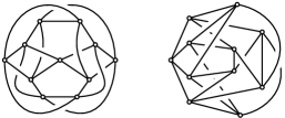
Figure 2. Knotless embeddings of graphs $H_{1}$ (left) and $H_{2}$ (right).

The Heawood family consists of twenty graphs of size 21 related to one another by $\nabla\mathrm{Y}$ and $\mathrm{Y}\nabla$ moves, see Figure 3. In [GMN, HNTY] two groups, working independently, verified that 14 of the graphs in the family are MMIK, and the remaining six are MMN2A and not MMIK. In subsection 3.2 below, we argue that no size 23 expansion of any of these six Heawood family graphs is MMIK.

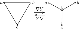
Figure 3. $\nabla\mathrm{Y}$ and $\mathrm{Y}\nabla$ moves.

Combining the arguments of the next three subsections give a proof of Theorem 1.1.

Before diving into the details, we state a few lemmas we’ll use throughout. The first is about the minimal degree $\delta(G)$, which is the least degree among the vertices of graph $G$.

Lemma 3.3.

If $G$ is MMIK, then $\delta(G)\geq 3$.

Proof.

Suppose $G$ is IK with $\delta(G)<3$. By either deleting, or contracting an edge on, a vertex of small degree, we find a proper minor that is also IK. ∎

Lemma 3.4.

The $\nabla\mathrm{Y}$ move preserves IK: If $G$ is IK and $H$ is obtained from $G$ by a $\nabla\mathrm{Y}$ move, then $H$ is also IK. Conversely, the $\mathrm{Y}\nabla$ move preserves nIK: if $H$ is nIK and $G$ is obtained from $H$ by a $\mathrm{Y}\nabla$ move, then $G$ is also nIK.

Proof.

Sachs [Sc] showed that $\mathrm{Y}\nabla$ preserves linkless embedding and essentially the same argument applies to knotless embeddings. ∎

Finally, we note that the MMIK property can move backwards along $\nabla\mathrm{Y}$ moves.

Lemma 3.5.

[BDLST, OT] Suppose $G$ is IK and $H$ is obtained from $G$ by a $\nabla\mathrm{Y}$ move. If $H$ is MMIK, then $G$ is also.

3.1. Proof of Theorem 3.2

In this subsection we prove Theorem 3.2: the three graphs $G_{1}$, $G_{2}$, and $G_{3}$ are MMIK.

3.1.1. $G_{1}$ is MMIK

To show that $G_{1}$ is MMIK, we first argue that no proper minor is IK. Up to isomorphism, there are 12 minors obtained by contracting or deleting a single edge. Each of these is 2-apex, except for the MMN2A graph $H_{1}$. By Lemma 3.1, a 2-apex graph is nIK and Figure 2 gives a knotless embedding of $H_{1}$. (Note that we use software to check that every cycle is a trivial knot in our knotless embeddings. A Mathematica version of the program is available at Ramin Naimi’s homepage [N2].) This shows that all proper minors of $G_{1}$ are nIK.

We next show that $G_{1}$ is IK. For this we use a lemma due, independently, to two groups [F, TY]. Let $\mathcal{D}_{4}$ denote the multigraph of Figure 4 and, for $i=1,2,3,4$, let $C_{i}$ be the cycle of edges $e_{2i-1},e_{2i}$. For any given embedding of $\mathcal{D}_{4}$, let $\sigma$ denote the mod 2 sum of the Arf invariants of the 16 Hamiltonian cycles in $\mathcal{D}_{4}$ and $\mbox{lk}(C,D)$ the mod 2 linking number of cycles $C$ and $D$. Since the Arf invariant of the unknot is zero, an embedding of $\mathcal{D}_{4}$ with $\sigma\neq 0$ must have a knotted cycle.

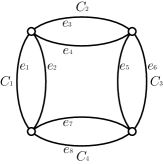
Figure 4. The $\mathcal{D}_{4}$ graph.

Lemma 3.6.

[F, TY] Given an embedding of $\mathcal{D}_{4}$, $\sigma\neq 0$ if and only if $\mbox{lk}(C_{1},C_{3})\neq 0$ and $\mbox{lk}(C_{2},C_{4})\neq 0$.

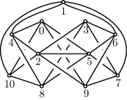
Figure 5. The graph $G_{1}$.

To use Lemma 3.6 we need pairs of linked cycles. We will find minors of $G_{1}$ that are members of the Petersen family of graphs as these are the obstructions to linkless embedding [RST]. For example, contracting edges $(3,6)$, $(5,7)$, and $(6,9)$ in Figure 5 yields a $K_{4,4}$ minor with $\{3,4,5,10\}$ and $\{0,1,2,8\}$ as the two parts. For convenience, we use the smallest vertex label to denote the new vertex obtained when contracting edges. Thus, we denote by 3 the vertex obtained by identifying 3, 6, and 9 of $G_{1}$. Further deleting the edge $(1,3)$ we identify the Petersen family graph $K_{4.4}^{-}$ as a minor of $G_{1}$.

There are nine pairs of disjoint cycles in $K_{4,4}^{-}$ and we will denote these pairs as $A_{1}$ through $A_{9}$. In Table 8, we first give the cycle pair in the $K_{4,4}^{-}$ and then the corresponding pair in $G_{1}$.

$A_{1}$	0,4,1,5 – 2,3,8,10	0,4,1,7,5 – 2,3,8,10
$A_{2}$	0,4,1,10 – 2,3,8,5	0,4,1,10 – 2,3,8,5
$A_{3}$	1,4,2,5 – 0,3,8,10	1,4,2,5,7 – 0,9,6,3,8,10
$A_{4}$	1,4,2,10 – 0,3,8,5	1,4,2,10 – 0,9,6,3,8,5
$A_{5}$	1,4,8,5 – 0,3,2,10	1,4,8,5,7 – 0,9,6,3,2,10
$A_{6}$	1,4,8,10 – 0,3,2,5	1,4,8,10 – 0,9,6,3,2,5
$A_{7}$	1,5,2,10 – 0,3,8,4	1,7,5,2,10 – 0,9,6,3,8,4
$A_{8}$	0,5,1,10 – 2,3,8,4	0,5,7,1,10 – 2,3,8,4
$A_{9}$	1,5,8,10 – 0,3,2,4	1,7,5,8,10 – 0,9,6,3,2,4

Table 8. Nine pairs of cycles in $G_{1}$ called $A_{1},\ldots,A_{9}$.

Similarly, we will describe a $K_{3,3,1}$ minor that gives pairs of cycles $B_{1}$ through $B_{9}$. Contract edges $(0,9)$, $(1,7)$, $(2,3)$, $(3,7)$, $(3,8)$, $(5,7)$, and $(7,9)$. Delete vertex $6$ and edge $(2,9)$. The result is a $K_{3,3,1}$ minor with parts $\{0,2,8\}$, $\{4,5,10\}$, and $\{1\}$. In Table 9 we give the nine pairs of cycles, first in $K_{3,3,1}$ and then in $G_{1}$.

$B_{1}$	0,1,4 – 2,5,8,10	0,4,1,7,9 – 2,5,8,10
$B_{2}$	0,1,5 – 2,4,8,10	0,5,7,9 – 2,4,8,10
$B_{3}$	0,1,10 – 2,4,8,5	0,9,7,1,10 – 2,4,8,5
$B_{4}$	1,2,4 – 0,5,8,10	1,4,2,3,7 – 0,5,8,10
$B_{5}$	1,2,5 – 0,4,8,10	2,3,7,5 – 0,4,8,10
$B_{6}$	1,2,10 – 0,4,8,5	2,3,7,1,10 – 0,4,8,5
$B_{7}$	1,4,8 – 0,5,2,10	1,4,8,3,7 – 0,5,2,10
$B_{8}$	1,5,8 – 0,4,2,10	3,7,5,8 – 0,4,2,10
$B_{9}$	1,8,10 – 0,4,2,5	1,7,3,8,10 – 0,4,2,5

Table 9. Nine pairs of cycles in $G_{1}$ called $B_{1},\ldots,B_{9}$.

Another $K_{4,4}^{-}$ minor of $G_{1}$ will give our last set of nine cycle pairs. Contract edges $(0,9)$, $(2,5)$, and $(3,8)$ to obtain a $K_{4,4}$ with parts $\{0,1,2,8\}$ and $\{4,6,7,10\}$. Then delete edge $(1,4)$ to make a $K_{4.4}^{-}$ minor. Table 10 lists the nine pairs of cycles, first in the $K_{4,4}^{-}$ minor and then in $G_{1}$.

$C_{1}$	0,6,1,7 – 2,4,8,10	9,6,1,7 – 2,4,8,10
$C_{2}$	0,6,1,10 – 2,4,8,7	0,9,6,1,10 – 2,4,8,3,7,5
$C_{3}$	1,6,2,7 – 0,4,8,10	1,6,5,7 – 0,4,8,10
$C_{4}$	1,6,2,10 – 0,4,8,7	1,6,5,2,10 – 0,4,8,3,7,9
$C_{5}$	1,6,8,7 – 0,4,2,10	1,6,,3,7 – 0,4,2,10
$C_{6}$	1,6,8,10 – 0,4,2,7	1,6,3,8,10 – 0,4,2,5,7,9
$C_{7}$	0,7,1,10 – 2,4,8,6	0,9,7,1,10 – 2,4,8,3,6,5
$C_{8}$	1,7,2,10 – 0,4,8,6	1,7,5,2,10 – 0,4,8,3,6,9
$C_{9}$	1,7,8,10 – 0,4,2,6	1,7,3,8,10 – 0,4,2,5,6,9

Table 10. Nine pairs of cycles in $G_{1}$ called $C_{1},\ldots,C_{9}$.

As shown by Sachs [Sc], in any embedding of $K_{4,4}^{-}$ or $K_{3,3,1}$, at least one pair of the nine disjoint cycles in each graph has odd linking number. We will simply say the cycles are linked if the linking number is odd. Fix an embedding of $G_{1}$. Our goal is to show that the embedding must have a knotted cycle.

We will argue by contradiction. For a contradiction, assume that there is no knotted cycle in the embedding of $G_{1}$. We leverage Lemma 3.6 to deduce that certain pairs of cycles are not linked. Eventually, we will conclude that none of $B_{1},\ldots,B_{9}$ are linked. This is a contradiction as these correspond to cycles in a $K_{3,3,1}$ and we know that every embedding of this Petersen family graph must have a pair of linked cycles [Sc]. The contradiction shows that there must in fact be a knotted cycle in the embedding of $G_{1}$. As the embedding is arbitrary, this shows that $G_{1}$ is IK.

We illustrate our strategy by first focusing on the pair $A_{2}=$ 0,4,1,10 – 2,3,8,5. Combine $A_{2}$ with each $B_{i}$. In each case we form a $\mathcal{D}_{4}$ graph as in Figure 4. Since the $B_{i}$ are pairs of cycles in $K_{3,3,1}$, a Petersen family graph, at least one pair is linked [Sc]. If $A_{2}$ is also linked, then Lemma 3.6 implies that the embedding of $G_{1}$ has a knotted cycle, in contradiction to our assumption. Therefore, we conclude that $A_{2}$ is not linked (i.e., does not have odd linking number).

$B_{1}$	$\{0,1,4\}$, $\{2,5,8\}$, $\{3,7\}$, $\{10\}$
$B_{2}$	$\{0\}$, $\{1,4,10\}$, $\{2,3,8\}$, $\{5\}$
$B_{3}$	$\{0,1,10\}$, $\{2,5,8\}$, $\{3,7\}$, $\{4\}$
$B_{4}$	$\{0,10\}$, $\{1,4\}$, $\{2,3\}$, $\{5,8\}$
$B_{5}$	$\{0,4,10\}$, $\{1\}$, $\{2,3,5\}$, $\{8\}$
$B_{6}$	$\{0,4\}$, $\{1,10\}$, $\{2,3\}$, $\{5,8\}$
$B_{7}$	$\{0,10\}$, $\{1,4\}$, $\{2,5\}$, $\{3,8\}$
$B_{8}$	$\{0,4,10\}$, $\{1,7\}$, $\{2\}$, $\{3,8,5\}$
$B_{9}$	$\{0,4\}$, $\{1,10\}$, $\{2,5\}$, $\{3,8\}$

Table 11. Pairing $A_{2}$ with $B_{1},\ldots,B_{9}$.

In Table 11, we list the vertices in $G_{1}$ that are identified to give each of the four vertices of $\mathcal{D}_{4}$. Let’s examine the pairing with $B_{2}$ as an example to see how this results in a $\mathcal{D}_{4}$. We identify $\{1,4,10\}$ as a single vertex by contracting edges $(1,4)$ and $(1,10)$. Similarly contract $(2,3)$ and $(3,8)$ to make a vertex of the $\mathcal{D}_{4}$ from vertices $\{2,3,8\}$ of $G_{1}$. In this way, the cycle 0,4,1,10 of $A_{2}$ in $G_{1}$ becomes cycle $C_{1}$ of the $\mathcal{D}_{4}$ (see Figure 4) between $\{1,4,10\}$ and $\{0\}$ and the cycle 2,3,8,5 becomes cycle $C_{3}$ between $\{2,3,8\}$ and $\{5\}$. Similarly 0,5,7,9 of $B_{2}$ becomes homeomorphic to the cycle $C_{2}$ between $\{0\}$ and $\{5\}$. For the final cycle of $B_{2}$, 2,4,8,10, we observe that, in homology, $\mbox{2,4,8,10 }=\mbox{ 1,4,2,10 }\cup\mbox{ 1,4,8,10}$. Assuming $\mbox{lk}((\mbox{0,5,7,9}),(\mbox{ 2,4,8,10}))\neq 0$, then one of $\mbox{lk}((\mbox{0,5,7,9}),(\mbox{1,4,2,10}))$ and $\mbox{lk}((\mbox{0,5,7,9}),(\mbox{1,4,8,10}))$ is also nonzero. Whichever it is, 1,4,2,10 or 1,4,8,10, that will be our $C_{4}$ cycle in the $\mathcal{D}_{4}$ of Figure 4.

To summarize, we’ve argued that $A_{2}$ forms a $\mathcal{D}_{4}$ with each pair $B_{1},\ldots,B_{9}$. Since at least one of the $B_{i}$’s is linked, then, assuming $A_{2}$ is linked, these two pairs make a $\mathcal{D}_{4}$ that has a knotted cycle. Therefore, by way of contradiction, going forward, we may assume $A_{2}$ is not linked.

We next argue that $A_{6}$ is not linked. Pairing with the $B_{i}$’s again, the vertices for each $\mathcal{D}_{4}$ are

$$B_{1} \{0,9\},\{1,4\},\{2,5\},\{8,9\} B_{2} \{0,5,9\},\{1,7\},\{2\},\{4,8,10\}$$

$$B_{3} \{0,9\},\{1,10\},\{2,5\},\{4,8\} B_{4} \{0,5\},\{1,4\},\{2,3\},\{8,10\}$$

$$B_{5} \{0\},\{1,7\},\{2,3,5\},\{4,8,10\} B_{6} \{0,5\},\{1,10\},\{2,3\},\{4,8\}$$

$$B_{7} \{0,2,5\},\{1,4,8\},\{3\},\{10\} B_{9} \{0,2,5\},\{1,8,10\},\{3\},\{4\}.$$

For $B_{8}=$ 3,7,5,8 – 0,4,2,10, we first split one of the $A_{6}$ cycles: $\mbox{0,5,2,3,6,9 }=\mbox{ 0,5,2,9 }\cup\mbox{ 2,3,6,9}$. One of the two summands must link with the other $A_{2}$ cycle $1,4,8,10$. If $\mbox{lk}((\mbox{0,5,2,9}),(\mbox{1,4,8,10}))\neq 0$, then, by a symmetry of $G_{1}$, $\mbox{lk}((\mbox{8,5,2,3}),(\mbox{1,4,0,10}))\neq 0$. But this last is the pair $A_{2}$, and we have already argued that $A_{2}$ is not linked.

Therefore, it must be that $\mbox{lk}((\mbox{2,3,6,9}),(\mbox{1,4,8,10}))\neq 0$. Next, we split a cycle of $B_{8}$: $\mbox{0,4,2,10 }=\mbox{ 1,4,2,10 }\cup\mbox{ 0,4,1,10}$. If $\mbox{lk}((\mbox{3,7,5,8}),(\mbox{1,4,2,10}))\neq 0$, form a $\mathcal{D}_{4}$ with vertices $\{1,4,10\}$, $\{2\}$, $\{3\}$, and $\{8\}$. On the other hand, If $\mbox{lk}((\mbox{3,7,5,8}),(\mbox{0,4,1,10}))\neq 0$, form a $\mathcal{D}_{4}$ with vertices $\{0,9\}$, $\{1,4,10\}$, $\{3\}$, and $\{8\}$.

For every choice of $B_{i}$ we can make a $\mathcal{D}_{4}$ with $A_{6}$. We know that at least one $B_{i}$ is a linked pair. If $A_{6}$ is also linked, then, by Lemma 3.6, this embedding of $G_{1}$ has a knotted cycle. Therefore, by way of contradiction, we may assume the pair of $A_{6}$ is not linked.

We next eliminate $B_{2}$ by pairing it with each $A_{i}$. As we’re assuming $A_{2}$ and $A_{6}$ are not linked, it must be some other $A_{i}$ pair that is linked. Here are the vertices of the $\mathcal{D}_{4}$’s in each case:

$$A_{1} \{0,5,7\},\{2,8,10\},\{3,6,9\},\{4\} A_{3} \{0,9\},\{2,4\},\{5,7\},\{8,10\}$$

$$A_{4} \{0,5,9\},\{1,7\},\{2,4,10\},\{8\} A_{5} \{0,9\},\{2,10\},\{4,8\},\{5,7\}$$

$$A_{7} \{0,9\},\{2,10\},\{4,8\},\{5,7\} A_{8} \{0,5,7\},\{2,4,8\},\{3,6,9\},\{10\}$$

$$A_{9} \{0,9\},\{2,4\},\{5,7\},\{8,10\}.$$

This shows $B_{2}$ is not linked. Since $B_{8}$ is the same as $B_{2}$ by a symmetry of $G_{1}$, $B_{8}$ is likewise not linked. Ultimately, we will show that no $B_{i}$ is linked. So far, we have this for $B_{2}$ and $B_{8}$.

Our next step is to argue $C_{1}$ is not linked by pairing it with the remaining $A_{i}$’s:

$$A_{1} \{1,7\},\{2,8,10\},\{3,6\},\{4\} A_{3} \{1,7\},\{2,4\},\{6,9\},\{8,10\}$$

$$A_{4} \{1\},\{2,4,10\},\{6,9\},\{8\} A_{5} \{1,7\},\{2,10\},\{4,8\},\{6,9\}$$

$$A_{7} \{0,4,8\},\{1,5,7\},\{6\},\{10\} A_{8} \{1,7\},\{2,4,8\},\{3,6\},\{10\}$$

$$A_{9} \{1,7\},\{2,4\},\{6,9\},\{8,10\}.$$

By a symmetry of $G_{1}$, $C_{5}$ is also not linked.

Now we argue that $C_{3}$ is not linked, again by pairing with $A_{i}$’s:

$$A_{1} \{0,4\},\{1,5,7\},\{3,6\},\{8,10\} A_{3} \{0,8,10\},\{1,5,7\},\{4\},\{6\}$$

$$A_{5} \{0,10\},\{1,5,7\},\{4,8\},\{6\} A_{7} \{0,4,8\},\{1,5,7\},\{6\},\{10\}$$

$$A_{8} \{0,10\},\{1,5,7\},\{4,8\},\{6\} A_{9} \{0,4\},\{1,5,7\},\{6\},\{8,10\}.$$

For $A_{4}$ we split the second cycle: $\mbox{0,9,6,3,8,5 }=\mbox{ 0,9,6,5 }\cup\mbox{ 6,3,8,5}$. Suppose that it’s 0,9,6,5 that is linked with 1,4,2,10. In this case we also split that cycle: $\mbox{1,4,2,10 }=\mbox{ 1,4,8,10 }\cup\mbox{ 2,4,8,10}$. To get a $\mathcal{D}_{4}$ when pairing 0,9,6,5 – 1,4,8,10 with $C_{3}$ we use vertices $\{0\}$, $\{1\}$, $\{4,8,10\}$, and $\{5,6\}$ and for 0,9,6,5 – 2,4,8,10 with $C_{3}$, $\{0\}$, $\{2,3,7\}$, $\{4,8,10\}$, and $\{5,6\}$.

On the other hand, if it’s 6,3,8,5 that’s linked with 1,4,2,10, we write $\mbox{1,4,2,10 }=\mbox{ 0,4,1,10 }\cup\mbox{ 0,4,2,10}$. Then when $C_{3}$ is paired with 6,3,8,5 — 0,4,1,10, we have a $\mathcal{D}_{4}$ using vertices $\{0,4,10\}$, $\{1\}$, $\{5,6\}$, and $\{8\}$ while if $C_{3}$ is paired with 6,3,8,5 – 0,4,2,10 the vertices are $\{0,4,10\}$, $\{2,7,9\}$, $\{5,6\}$, and $\{8\}$. This completes the argument that $C_{3}$ is not linked.

We will show that $A_{8}$ is not linked by pairing with the remaining $C_{i}$’s. For $C_{8}$, the vertices would be $\{0\}$, $\{1,5,7,10\}$, $\{2\}$, and $\{3,4,8\}$. The remaining cases involve splitting cycles.

For $C_{2}$ we write $\mbox{2,4,8,3,7,5 }=\mbox{ 3,7,5,8 }\cup\mbox{ 2,4,8,5}$. If it’s 3,7,5,8 – 0,9,6,1,10 that’s linked, we use vertices $\{0,1,10\}$, $\{2,9\}$, $\{3,8\}$, and $\{5,7\}$ and if, instead, 2,4,8,5 – 0,9,6,10 is linked, we have $\{0,1,10\}$, $\{2,4,8\}$, $\{3,6\}$, and $\{5\}$.

For $C_{4}$, it’s a cycle of $A_{8}$ that we rewrite: $\mbox{0,5,7,1,10 }=\mbox{ 0,9,7,1,10 }\cup\mbox{ 0,9,7,5}$. In either case, we use the same vertices: $\{0,7,9\}$, $\{1,5,6,10\}$, $\{2\}$, and $\{3,4,8\}$.

For $C_{6}$, $\mbox{0,4,2,5,7,9 }=\mbox{ 0,4,2,9 }\cup\mbox{ 2,5,7,9}$. When 0,4,2,9 is linked with 1,6,3,8,10 the vertices are $\{0,9\}$, $\{1,10\}$, $\{2,4\}$, and $\{3,8\}$ while if 2,5,7,9 links 1,6,3,8,10, we use $\{1,10\}$, $\{2\}$, $\{3,8\}$, and $\{5,7\}$.

Continuing with $C_{7}$, $\mbox{2,4,8,3,6,5 }=\mbox{ 3,6,5,8 }\cup\mbox{ 2,4,8,5}$. The vertices for 3,6,5,8 – 0,9,7,1,0 are $\{0,1,7,10\}$, $\{2,9\}$, $\{3,8\}$, and $\{5\}$ and for 2,4,8,5 – 0,9,7,1,10, use $\{0,1,7,10\}$, $\{2,4,8\}$, $\{3,6,9\}$, and $\{5\}$.

Finally, in the case of $C_{9}$, write $\mbox{0,4,2,5,6,9 }=\mbox{ 0,4,2,9 }\cup\mbox{ 2,5,6,9}$. When 0,4,2,9 – 1,7,3,8,10 is linked, the vertices are $\{0\}$, $\{1,7,10\}$, $\{2,4\}$, and $\{3,8\}$ and for 2,5,6,9 – 1,7,3,8,10 use $\{1,7,10\}$, $\{2\}$, $\{3,8\}$, and $\{5\}$. This completes the argument for $A_{8}$. By a symmetry of $G_{1}$, $A_{1}$ is also not linked. In other words, going forward, we will assume it is one of $A_{3}$, $A_{4}$, $A_{5}$, $A_{7}$, or $A_{9}$ that is linked.

Next, we’ll argue that $B_{1}$ is not linked by comparing with the remaining $A_{i}$’s:

$$A_{3} \{0,9\},\{1,4,7\},\{2,5\},\{8,10\} A_{4} \{0,9\},\{1,4\},\{2,10\},\{5,8\}$$

$$A_{5} \{0,9\},\{1,4,7\},\{2,10\},\{5,8\} A_{7} \{0,4,9\},\{1,7\},\{2,5,10\},\{8\}$$

$$A_{9} \{0,4,9\},\{1,7\},\{2\},\{5,8,10\}.$$

By a symmetry of $G_{1}$ we also assume $B_{3}$ is not linked.

Now, by pairing with the remaining $A_{i}$’s, we show $B_{5}$ is not linked:

$$A_{3} \{0,8,10\},\{2,5,7\},\{3\},\{4\} A_{5} \{0,10\},\{2,3\},\{4,8\},\{5,7\}$$

$$A_{7} \{0,4,8\},\{2,5,7\},\{3\},\{10\} A_{9} \{0,4\},\{2,3\},\{5,7\},\{8,10\}.$$

For $A_{4}$ we employ several splits. First, $\mbox{0,9,6,3,8,5 }=\mbox{ 0,9,6,5 }\cup\mbox{ 6,3,8,5}$. In the case that 0,9,6,5 – 1,4,2,10 is linked, write $\mbox{1,4,2,10 }=\mbox{ 2,4,8,10 }\cup\mbox{ 1,4,8,10}$. Pairing 0,9,6,5 – 2,4,8,10 with $B_{5}$, the vertices are $\{0\}$, $\{2\}$, $\{4,8,10\}$, and $\{5\}$. If instead it’s 0,9,6,5 – 1,4,8,10 that’s linked, we use $\{0\}$, $\{1,7\}$, $\{4,8,10\}$, and $\{5\}$.

So we assume that 6,3,8,5 – 1,4,2,10 is linked and rewrite a $B_{5}$ cycle: $\mbox{2,3,7,5 }=\mbox{ 2,3,6,5 }\cup\mbox{ 3,6,5,7}$. In case 2,3,6,5 – 0,4,8,10 is linked, we make a further split: $\mbox{1,4,2,10 }=\mbox{ 1,7,9,2,10 }\cup\mbox{ 1,4,9,2,10}$. Thus, assuming 2,3,6,5 – 0,4,8,10 and 1,7,9,2,10 – 6,3,8,5 are both linked, we have a $\mathcal{D}_{4}$ with vertices $\{2\}$, $\{3,5,6\}$, $\{8\}$, and $\{10\}$. If instead it’s 2,3,6,5 – 0,4,8,10 and 1,4,9,2,10 – 6,3,8,5 that are linked, use $\{2\}$, $\{3,5,6\}$, $\{4\}$, and $\{8\}$. This leaves the case where 3,6,5,7 – 0,4,8,10 is linked. We must split a final time: $\mbox{1,4,2,10 }=\mbox{ 0,4,1,10 }\cup\mbox{ 0,4,2,10}$. If 3,6,5,7 – 0,4,8,10 and 0,4,1,10 – 6,3,8,5 are both linked, the vertices are $\{0,4,10\}$, $\{1,7\}$, $\{3,5,6\}$, and $\{8\}$. On the other hand, when 3,6,5,7 – 0,4,8,10 and 0,4,2,10 – 6,3,8,5 are linked, use $\{0,4,10\}$, $\{2,7,9\}$, $\{3,5,6\}$, and $\{8\}$. This completes the argument for $B_{5}$, which we have shown is not linked.

Next we turn to $B_{9}$ which we compare with the remaining $A_{i}$’s:

$$A_{3} \{0\},\{1,7\},\{2,4,5\},\{3,8,10\} A_{4} \{0,5\},\{1,10\},\{2,4\},\{3,8\}$$

$$A_{7} \{0,4\},\{1,7,10\},\{2,5\},\{3,8\} A_{9} \{0,2,4\},\{1,7,8,10\},\{3\},\{5\}.$$

This leaves $A_{5}$ for which we rewrite: $\mbox{0,9,6,3,2,10 }=\mbox{ 0,9,2,10 }\cup\mbox{ 2,3,6,9}$. If 0,9,2,10 – 1,4,8,5,7 is linked, then observe that, by a symmetry of $G_{1}$, this is the same as $A_{8}$, which is not linked. Thus, we can assume 2,3,6,9 – 1,4,8,5,7 is linked and rewrite: $\mbox{1,4,8,5,7 }=\mbox{ 1,4,0,5,7 }\cup\mbox{ 0,4,8,5}$. Pairing 2,3,6,9 - 1,4,0,5,7 with $B_{9}$ gives a $\mathcal{D}_{4}$ on vertices $\{0,4,5\}$, $\{1,7\}$, $\{2\}$, and $\{3\}$. If it’s 2,3,6,9 – 0,4,8,5 that’s linked, then, pairing with $B_{9}$, use $\{0,4,5\}$, $\{2\}$, $\{3\}$, and $\{8\}$. This completes the argument for $B_{9}$ and, by a symmetry of $G_{1}$, also for $B_{7}$.

Recall that our goal is to argue, for a contradiction, that no $B_{i}$ is linked. At this stage we are left only with $B_{4}$ and $B_{6}$ as pairs that could be linked.

Before providing the argument for the remaining two $B_{i}$’s, we first eliminate a few more $A_{i}$’s, starting with $A_{4}$, which we compare with the two remaining $B_{i}$’s:

$$B_{4} \{0,5,8\},\{1,2,4\},\{3\},\{10\} B_{6} \{0,5,8\},\{1,2,10\},\{3\},\{4\}.$$

Next $A_{5}$, again by pairing with $B_{4}$ and $B_{6}$:

$$B_{4} \{0,10\},\{1,4,7\},\{2,3\},\{5,8\} B_{6} \{0\},\{1,7\},\{2,3,10\},\{4,8,5\}.$$

Since $A_{9}$ agrees with $A_{5}$ under a symmetry of $G_{1}$, this leaves only $A_{3}$ and $A_{7}$ as pairs that may yet be linked among the $A_{i}$’s.

As a penultimate step, we show that $C_{6}$ is not linked by comparing with these two remaining $A_{i}$’s:

$$A_{3} \{0,9\},\{1\},\{2,4,5,7\},\{3,6,8,10\} A_{7} \{0,4,9\},\{1,10\},\{2,5,7\},\{3,6,8\}.$$

By a symmetry of $G_{1}$, we can also assume that $C_{9}$ is not linked. This leaves only four $C_{i}$’s that may be linked: $C_{2}$, $C_{4}$, $C_{7}$, and $C_{8}$.

Finally, compare $B_{6}$ with the remaining $C_{i}$’s:

$$C_{4} \{0,4,8\},\{1,2,10\},\{3,7\},\{5\} C_{8} \{0,4,8\},\{1,2,7,10\},\{3\},\{5\}.$$

For $C_{2}$ we rewrite: $\mbox{2,4,8,3,7,5 }=\mbox{ 2,3,8,4 }\cup\mbox{ 2,3,7,5}$. If 2,3,8,4 – 0,9,6,1,10 is linked, then pairing with $B_{6}$, we have vertices $\{0\}$, $\{1,10\}$, $\{2,3\}$, and $\{4,8\}$. On the other hand pairing $B_{6}$ with 2,3,7,5 – 0,9,6,1,10 we’ll have a $\mathcal{D}_{4}$ using the vertices $\{0\}$, $\{1,10\}$, $\{2,3,7\}$, and $\{5\}$.

For $C_{7}$: $\mbox{2,4,8,3,6,5 }=\mbox{ 2,3,8,4 }\cup\mbox{ 2,3,6,5}$. Then 2,3,8,4 – 0,9,7,1,10 with $B_{6}$ gives a $\mathcal{D}_{4}$ for vertices $\{0\}$, $\{1,7,10\}$, $\{2,3\}$, and $\{4,8\}$. On the other hand, 2,3,6,5 – 0,9,7,1,10 pairs with $B_{6}$ using vertices $\{0\}$, $\{1,7,10\}$, $\{2,3\}$, and $\{5\}$.

This completes the argument for $B_{6}$. By a symmetry of $G_{1}$ we see that $B_{4}$ is also not linked.

In this way, the assumption that there is no knotted cycle in the given embedding of $G_{1}$ forces us to conclude that no pair $B_{1},\ldots,B_{9}$ is linked. However, these correspond to the cycles of a $K_{3,3,1}$. As Sachs [Sc] has shown, any embedding of $K_{3,3,1}$ must have a pair of cycles with odd linking number. The contradiction shows that there can be no such knotless embedding and $G_{1}$ is IK. This completes the proof that $G_{1}$ is MMIK.

3.1.2. $G_{2}$ is MMIK

Again, we must argue that $G_{2}$ is IK, and every proper minor is nIK. Up to isomorphism, there are 26 minors obtained by deleting or contracting an edge of $G_{2}$. Each of these is 2-apex but for the graph $H_{2}$, for which a knotless embedding is given in Figure 2. This shows that the proper minors of $G_{2}$ are nIK.

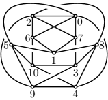
Figure 6. The graph $G_{2}$.

We will use Lemma 3.6 to show that $G_{2}$ is IK. The argument is similar to that for $G_{1}$ above. We begin by identifying four ways that the Petersen family graph $P_{9}$, of order nine, appears as a minor of graph $G_{2}$. Using the vertex labelling of Figure 6, on contracting edge $(0,4)$ and deleting vertex 8, the resulting graph has $P_{9}$ as a subgraph. We denote the seven cycle pairs in this minor $A1,\ldots,A7$ and list the corresponding links in $G_{2}$ in Table 12.

$A_{1}$	0,4,10,5 – 1,6,2,9,3,7
$A_{2}$	0,2,6,10,4 – 1,5,9,3,7
$A_{3}$	0,2,9,5 – 1,6,10,3,7
$A_{4}$	0,5,1,7 – 2,6,10,3,9
$A_{5}$	0,4,10,3,7 – 1,5,9,2,6
$A_{6}$	1,5,10,6 – 0,2,9,3,7
$A_{7}$	3,9,5,10 – 0,2,6,1,7

Table 12. Seven pairs of cycles in $G_{2}$ called $A_{1},\ldots,A_{7}$.

Similarly, if we contract edge $(3,10)$ and delete vertex 7 in $G_{2}$, the resulting graph has a $P_{9}$ subgraph. We’ll call these seven cycles $B_{1},\ldots B_{7}$ as in Table 13

$B_{1}$	0,2,6 – 1,5,9,3,10,4,8
$B_{2}$	0,2,8,4 – 1,5,9,3,10,6
$B_{3}$	0,2,9,5 – 1,6,10,4,8
$B_{4}$	0,4,10,6 – 1,5,9,2,8
$B_{5}$	0,5,1,6 – 2,8,4,10,3,9
$B_{6}$	1,6,2,8 – 0,4,10,3,9,5
$B_{7}$	2,6,10,3,9 – 0,4,8,1,5

Table 13. Seven pairs of cycles in $G_{2}$ called $B_{1},\ldots,B_{7}$.

Contracting edge $(4,10)$ and deleting vertex 6, we have the seven cycles of Table 14.

$C_{1}$	3,8,4,10 – 0,2,9,5,1,7
$C_{2}$	3,8,1,7 – 0,2,9,5,10,4
$C_{3}$	2,8,3,9 – 0,4,10,5,1,7
$C_{4}$	0,4,10,3,7 – 1,5,9,2,8
$C_{5}$	3,9,5,10 – 0,2,8,1,7
$C_{6}$	1,5,10,4,8 – 0,2,9,3,7
$C_{7}$	0,2,8,4 – 1,5,9,3,7

Table 14. Seven pairs of cycles in $G_{2}$ called $C_{1},\ldots,C_{7}$.

Finally, if we contract edge $(3,9)$ and delete vertex 7 in $G_{2}$, the resulting graph has a $P_{9}$ subgraph. We’ll call these seven cycles $D_{1},\ldots D_{7}$ as in Table 15.

$D_{1}$	2,8,3,9 – 0,4,10,6,1,5
$D_{2}$	0,2,9,5 – 1,6,10,4,8
$D_{3}$	0,2,8,4 – 1,5,9,3,10,6
$D_{4}$	1,5,9,3,8 – 0,2,6,10,4
$D_{5}$	1,6,2,8 – 0,4,10,3,9,5
$D_{6}$	3,8,4,10 – 0,2,6,1,5
$D_{7}$	2,6,10,3,9 – 0,4,8,1,5

Table 15. Seven pairs of cycles in $G_{2}$ called $D_{1},\ldots,D_{7}$.

We will need to introduce two more Petersen family graph minors later, but let’s begin by ruling out some of the pairs we already have. As in our argument for $G_{1}$, we assume that we have a knotless embedding of $G_{2}$ and step by step argue that various cycle pairs are not linked (i.e. do not have odd linking number) using Lemma 3.6. Eventually, this will allow us to deduce that all seven pairs $B_{1},\ldots,B_{7}$ are not linked. This is a contradiction since Sachs [Sc] showed that in any embedding of $P_{9}$, there must be a pair of cycles with odd linking number. The contradiction shows that there is no such knotless embedding and $G_{2}$ is IK.

We’ll see that $A_{5}$ is not linked by showing it results in a $\mathcal{D}_{4}$ with every pair $B_{1},\ldots,B_{7}$. Indeed the vertices of the $\mathcal{D}_{4}$ are formed by contracting the following vertices

$$B_{1} \{0\},\{1,5,9\},\{2,6\},\{3,4,10\} B_{2} \{0,4\},\{1,5,6,9\},\{2\},\{3,10\}$$

$$B_{3} \{0\},\{1,6\},\{2,5,9\},\{4,10\} B_{4} \{0,4,10\},\{1,2,5,9\},\{3,8\},\{6\}$$

$$B_{5} \{0\},\{1,5,6\},\{2,9\},\{3,4,10\} B_{7} \{0,4\},\{1,5\},\{2,6,9\},\{3,10\}.$$

For $B_{6}=$ 1,6,2,8 – 0,4,10,3,9,5, we first split one of the $A_{5}$ cycles: $\mbox{0,4,10,3,7 }=\mbox{0,4,8,3,7 }\cup\mbox{ 3,8,4,10}$. One of the two summands must link with the other $A_{5}$ cycle $1,5,9,2,6$. If $\mbox{lk}((\mbox{3,8,4,10}),(\mbox{1,5,9,2,6}))\neq 0$, then, by contracting edges, we form a $\mathcal{D}_{4}$ with $A_{5}$ whose vertices are $\{1,2,6\},\{3,4,10\},\{5,9\},\{8\}$. On the other hand, if $\mbox{lk}((\mbox{0,4,8,3,7}),(\mbox{1,5,9,2,6}))\neq 0$, then we will split the $B_{6}$ cycle $\mbox{0,4,10,3,9,5 }=\mbox{0,4,10,5 }\cup\mbox{ 3,9,5,10}$. When $\mbox{lk}((\mbox{1,6,2,8}),(\mbox{0,4,10,5}))\neq 0$, we have a $\mathcal{D}_{4}$ with vertices $\{0,4\},\{1,2,6\},\{5\},\{8\}$ and when $\mbox{lk}((\mbox{1,6,2,8}),$ $(\mbox{3,9,5,10}))\neq 0$, the $\mathcal{D}_{4}$ is on $\{1,2,6\},\{3\},\{5,9\},\{8\}$.

We have shown that, for each $B_{i}$, we must have a $\mathcal{D}_{4}$ with $A_{5}$. Sachs [Sc] showed that in every embedding of $P_{9}$, there is a pair of linked cycles. Thus, in our embedding of $G_{2}$, at least one $B_{i}$ is linked. If $A_{5}$ were also linked, that would result in a $\mathcal{D}_{4}$ with a knotted cycle by Lemma 3.6. This contradicts our assumption that we have a knotless embedding of $G_{2}$. Therefore, going forward, we can assume $A_{5}$ is not linked.

We next argue that $B_{7}$ is not linked by comparing with $C_{1},\ldots,C_{7}$. For $C_{4}$, $C_{6}$, and $C_{7}$, we immediately form a $\mathcal{D}_{4}$ as follows

$$C_{4} \{0,4\},\{1,5,8\},\{2,9\},\{3,7\} C_{6} \{0\},\{1,4,5,8\},\{2,3,9\},\{10\}$$

$$C_{7} \{0,4,8\},\{1,5\},\{2\},\{3,9\}.$$

For the remaining pairs, we will split a cycle of the $C_{i}$. For $C_{1}$, write $\mbox{0,2,9,5,1,7 }=\mbox{0,2,7 }\cup\mbox{ 1,5,9,2,7}$. In the first case, where $\mbox{lk}((\mbox{3,8,4,10}),$ $(\mbox{0,2,7}))\neq 0$, the $\mathcal{D}_{4}$ is on $\{0\},\{2\},\{3,10\},\{4,8\}$. In the second case, $\mbox{lk}((\mbox{3,8,4,10}),$ $(\mbox{1,5,9,7}))\neq 0$, we have $\{1,5\},\{2,9\},\{3,10\},\{4,8\}$.

For $C_{2}$, split $\mbox{0,2,9,5,10,4 }=\mbox{0,2,9,5 }\cup\mbox{ 0,4,10,5}$ with, in the first case, a $\mathcal{D}_{4}$ on $\{0,5\},\{1,8\},\{2,9\},\{3\}$ and, in the second, on $\{0,4,5\},\{1,8\},\{3\},\{10\}$. For $C_{5}$, $\mbox{0,2,8,1,7 }=\mbox{0,2,7 }\cup\mbox{ 1,7,2,8}$, the first case is $\{0\},\{2\},\{3,9,10\},\{5\}$ and the second has $\{1,8\},\{2\},\{3,9,10\},\{5\}$.

Finally, for $C_{3}$ split $\mbox{0,4,10,5,1,7 }=\mbox{1,6,7 }\cup\mbox{ 1,6,7,0,4,10,5}$. In the first case, there’s a $\mathcal{D}_{4}$ with vertices $\{1\},\{2,3,9\},\{6\},\{8\}$. In the second case, we split the same cycle a second time: $\mbox{1,6,7,0,4,10,5 }=\mbox{1,5,10,6 }\cup\mbox{ 0,4,10,6,7}$. In the first subcase, we have a $\mathcal{D}_{4}$ with vertices $\{1,5\},\{2,3,9\},\{6,10\},\{8\}$ and in the second subcase, $\{0,4\},\{2,3,9\},\{6,10\},\{8\}$.

Going forward, we can assume that $B_{7}$ is not linked.

We next argue that $A_{4}$ is not linked by comparing with $D_{1},\ldots,D_{7}$. For four links, we immediately give the vertices of the $\mathcal{D}_{4}$:

$$D2 \{0,5\},\{1\},\{2,9\},\{6,10\} D3 \{0\},\{1,5\},\{2\},\{3,6,9,10\}$$

$$D4 \{0\},\{1,5\},\{2,6,10\},\{3,9\} D5 \{0,5\},\{1\},\{2,6\},\{3,9,10\}.$$

For $D_{1}$, split the second cycle of $A_{4}$: $\mbox{2,6,10,3,9 }=\mbox{3,9,4,10 }\cup\mbox{ 2,9,4,10,6}$. In the first case, the verices of the $\mathcal{D}_{4}$ are $\{0,1,5\},\{2,7\},\{3,9\},\{4,10\}$ and in the second, $\{0,1,5\},\{2,9\},\{3,7\},\{4,6,10\}$. For $D_{6}$, split the second cycle: $\mbox{0,2,6,1,5 }=\mbox{0,2,9,5 }\cup\mbox{ 1,5,9,2,6}$. In the first case, we have vertices $\{0,5\},\{1,8\},\{2,9\},\{3,10\}$ and in the second, $\{0,4\},\{1,5\},\{2,6,9\},\{3,10\}$. Finally, $D_{7}$ is the same pair of cycles as $B_{7}$, which we have assumed is not linked. Going forward, we will assume $A_{4}$ is not linked.

We have already argued that we can assume $A_{4}$ and $A_{5}$ are not linked. Our next steps will eliminate $A_{2}$ and $A_{3}$, leaving only three $A_{i}$ that could be linked. For this we use another Petersen graph minor. Using the labelling of Figure 6, partition the vertices as $\{0,8,9,10\}$ and $\{2,3,4,5\}$. Contract edges $(0,7)$ and $(2,6)$. This resulting graph has a $K_{4,4}^{-}$ subgraph, where $(5,8)$ is the missing edge. As in Table 16, we’ll call the resulting nine pairs of cycles $E_{1},\ldots,E_{9}$.

$E_{1}$	2,8,4,9 – 0,5,10,3,7
$E_{2}$	0,4,10,5 – 2,8,3,9
$E_{3}$	0,2,6,10,5 – 3,8,4,9
$E_{4}$	0,2,4,8 – 3,9,5,10
$E_{5}$	4,9,5,10 – 0,2,8,3,7
$E_{6}$	0,4,8,3,7 – 2,6,10,5,9
$E_{7}$	0,5,9,3,7 – 2,6,10,4,8
$E_{8}$	0,4,9,5 – 2,6,10,3,8
$E_{9}$	0,2,9,5 – 3,8,4,10

Table 16. Nine pairs of cycles in $G_{2}$ called $E_{1},\ldots,E_{9}$.

We will use $E_{1},\ldots,E_{9}$ to show that $A_{2}$ may be assumed unlinked. Except for $E_{1}$, we list the vertices of the $\mathcal{D}_{4}$:

$$E_{2} \{0,4,10\},\{2\},\{3,9\},\{5\} E_{3} \{0,2,6,10\},\{3,9\},\{4\},\{5\}$$

$$E_{4} \{0,2,4\},\{1,8\},\{3,5,9\},\{10\} E_{5} \{0,2\},\{3,7\},\{4,10\},\{5,9\}$$

$$E_{6} \{0,4\},\{2,6,10\},\{3,7\},\{5,9\} E_{7} \{0\},\{1,8\},\{2,4,6,10\},\{3,5,7,9\}$$

$$E_{8} \{0,4\},\{2,6,10\},\{3\},\{5,9\} E_{9} \{0,2\},\{3\},\{4,10\},\{5,9\}.$$

The argument for $E_{1}$ is a little involved. Let’s split the second cycle $\mbox{0,5,10,3,7 }=\mbox{0,5,10,6,1,7 }\cup\mbox{ 1,6,10,3,7}$.

Case 1: Suppose that $\mbox{lk}((\mbox{2,8,4,9}),(\mbox{0,5,10,6,1,7}))\neq 0$. Next split the first cycle of $A_{2}$: $\mbox{0,2,6,10,4 }=\mbox{0,2,6 }\cup\mbox{ 0,4,10,6}$.

Case 1a): Suppose that $\mbox{lk}((\mbox{0,2,6}),(\mbox{1,5,9,3,7}))\neq 0$. We split the second $E_{1}$ cycle again: $\mbox{0,5,10,6,1,7 }=\mbox{0,5,10,6 }\cup\mbox{ 0,6,1,7}$ In the first case, where $\mbox{lk}((\mbox{2,8,4,9}),(\mbox{0,5,10,6}))\neq 0$, we have a $\mathcal{D}_{4}$ with vertices $\{0,6\},\{2\},\{5\},\{9\}$. In the second case, $\mbox{lk}((\mbox{2,8,4,9}),(\mbox{0,6,1,7}))\neq 0$, the $\mathcal{D}_{4}$ vertices are $\{0,6\},\{1,7\},$ $\{2\},\{9\}$.

Case 1b): Suppose that $\mbox{lk}((\mbox{0,4,10,6}),(\mbox{1,5,9,3,7}))\neq 0$. Split the second $E_{1}$ cycle again: $\mbox{0,5,10,6,1,7 }=\mbox{0,5,10,6 }\cup\mbox{ 0,6,1,7}$. In the first case, where $\mbox{lk}((\mbox{2,8,4,9}),(\mbox{0,5,10,6}))\neq 0$, the $\mathcal{D}_{4}$ vertices are $\{0,6,10\},\{4\},\{5\},\{9\}$. In the second case, where $\mbox{lk}((\mbox{2,8,4,9}),(\mbox{0,6,1,7}))\neq 0$, we have vertices $\{0,6\},\{1,7\},$ $\{4\},\{9\}$.

Case 2: Suppose that $\mbox{lk}((\mbox{2,8,4,9}),(\mbox{1,6,10,3,7}))\neq 0$. We split the fist cycle of $A_{2}$: $\mbox{0,2,6,10,4 }=\mbox{0,2,6 }\cup\mbox{ 0,4,10,6}$. In the first case, the $\mathcal{D}_{4}$ has vertices $\{1,3,7\},\{2\},\{6\},\{9\}$ and in the second $\{1,3,7\},\{4\},\{6,10\},\{9\}$.

This completes the argument for $A_{2}$, which we henceforth assume is not linked.

Next we again use $E_{1},\ldots,E_{9}$ to see that $A_{3}$ is also not linked. Except for $E_{8}$ and $E_{9}$ we immediately have a $\mathcal{D}_{4}$:

$$E_{1} \{0,5\},\{1,8\},\{2,9\},\{3,7,10\} E_{2} \{0,5\},\{2,9\},\{3\},\{10\}$$

$$E_{3} \{0,2,5\},\{3\},\{6\},\{9\} E_{4} \{0,2\},\{1,8\},\{3,10\},\{5,9\}$$

$$E_{5} \{0,2\},\{3,7\},\{5,9\},\{10\} E_{6} \{0\},\{2,5,9\},\{3,7\},\{6,10\}$$

$$E_{7} \{0,5,9\},\{2\},\{3,7\},\{6,10\}$$

For $E_{8}$, split the first cycle $\mbox{0,4,9,5 }=\mbox{0,5,1,7 }\cup\mbox{ 0,4,9,5,1,7}$. In the first case, we have a $\mathcal{D}_{4}$ with vertices $\{0,5\},\{1,7\},\{2\},\{3,6,10\}$. In the second case, we further split the first cycle of $A_{3}$: $\mbox{0,2,9,5 }=\mbox{2,8,4,9 }\cup\mbox{ 0,2,8,4,9,5}$ leading to two subcases. In the first subcase the $\mathcal{D}_{4}$ is $\{1,7\},\{2,8\},\{3,6,10\},\{4,9\}$ and in the second $\{0,4,5,9\},\{1,7\},\{2,8\},\{3,6,10\}$.

For $E_{9}$ split the first cycle $\mbox{0,2,9,5 }=\mbox{0,2,6,1,5 }\cup\mbox{ 2,6,1,5,9}$ with a $\mathcal{D}_{4}$ on first $\{0,2,5\},\{1,6\},\{3,10\},\{4,9\}$ and then $\{0,4\},\{1,6\},\{2,5,9\},\{3,10\}$.

We will not need $E_{1},\ldots,E_{9}$ in the remainder of the argument. At this stage, we can assume that it is one of $A_{1}$, $A_{6}$, and $A_{7}$ that is linked.

Our next step is to argue that we can assume $B_{5}$ is not linked by comparing with the three remaining $A_{i}$’s. For the first two, we immediately recognize a $\mathcal{D}_{4}$:

$$A_{1} \{0,5\},\{1,6\},\{2,3,9\},\{4,10\} A_{6} \{0\},\{1,5,6\},\{2,3,9\},\{10\}$$

For $A_{7}$, split the second cycle: $\mbox{0,2,6,1,7 }=\mbox{0,2,7 }\cup\mbox{ 2,6,1,7}$ so that the $\mathcal{D}_{4}$ has vertices $\{0\},\{2\},\{3,9,10\},\{5\}$ in the first case and then $\{1,6\},\{2\},$ $\{3,9,10\},\{5\}$. Going forward, we assume that $B_{5}$ is not linked.

Next we will eliminate $B_{2}$ and $B_{3}$. For $B_{3}$, we have a $\mathcal{D}_{4}$ with each of the remaining $A_{i}$’s:

$$A_{1} \{0,5\},\{1,6\},\{2,9\},\{4,10\} A_{6} \{0,2,9\},\{1,6,10\},\{3,8\},\{5\}$$

$$A_{7} \{0,2\},\{1,6\},\{5,9\},\{10\}$$

For $B_{2}$, notice first that, as we are assuming $A_{3}$ is not linked, by a symmetry of $G_{2}$, we can assume that 0,2,8,4 - 1,6,10,3,7 is also not linked. Again, since $B_{3}$ is unlinked, the symmetric pair 0,2,8,4 - 1,5,9,3,7 is also not linked. Since $\mbox{1,5,9,3,10,6 }=\mbox{1,5,9,3,7 }\cup\mbox{ 1,6,10,3,7}$ we conclude that $B_{2}$ is not linked. Having eliminated four of the $B_{i}$’s, going forward, we can assume that it is one of $B_{1}$, $B_{4}$, and $B_{6}$ that is linked. Recall that our ultimate goal is to argue that none of the $B_{i}$ are linked and thereby force a contradiction.

Our next step is to argue that $C_{1}$ is not linked by comparing with the remaining three $A_{i}$’s. For $A_{1}$ split the second cycle of $C_{1}$ $\mbox{0,2,9,5,1,7 }=\mbox{0,2,9,5 }\cup\mbox{ 0,5,1,7}$, yielding first a $\mathcal{D}_{4}$ on $\{0,5\},\{2,9\},\{3\},\{4,10\}$ and then on $\{0,5\},\{1,7\},\{3\},\{4,10\}$. For $A_{6}$, we have $\mathcal{D}_{4}$ with vertices $\{0,2,7,9\},\{1,5\},$ $\{3\},\{10\}$.

For $A_{7}$, split the second cycle $\mbox{0,2,6,1,7 }=\mbox{0,2,8,1,7 }\cup\mbox{ 1,6,2,8}$. In the first case, we have a $\mathcal{D}_{4}$ with vertices $\{0,1,2,7\},\{3,10\},\{5,9\},\{8\}$. In the second case, split the second cycle of $C_{1}$ $\mbox{0,2,9,5,1,7 }=\mbox{0,2,9,5 }\cup\mbox{ 0,5,1,7}$, resulting in a $\mathcal{D}_{4}$ either on $\{2\},\{3,10\},\{5,9\},\{8\}$ or $\{1\},\{3,10\},\{5\},\{8\}$.

Now we can eliminate $A_{7}$. Using a symmetry of $G_{2}$ we will instead argue that the pair $A_{7}^{\prime}$ = 3,8,4,10 - 0,2,6,1,7 is not linked. Note that this resembles $C_{1}$, which we just proved unlinked. Since $\mbox{0,2,6,1,7 }\cup\mbox{ 0,2,9,5,1,7 }=\mbox{1,5,9,2,6}$ it will be enough to show that 3,8,4,10 - 1,5,9,2,6 is not linked by comparing with the remaining $A_{i}$’s:

$$A_{1} \{1,2,6,9\},\{3\},\{4,10\},\{5\} A_{6} \{1,5,6\},\{2,9\},\{3\},\{10\}$$

$$A_{7} \{0,4\},\{1,2,6\},\{3,10\},\{5,9\}$$

Thus we can assume that it is $A_{1}$ or $A_{6}$ that is the linked pair in our embedding of $G_{2}$.

As for the $B_{i}$’s, only three candidates remain. We next eliminate $B_{1}$ by comparing with the remaining two $A_{i}$’s. For $A_{1}$, split the second cycle of $B_{1}$: $\mbox{1,5,9,3,10,4,8 }=\mbox{1,5,10,4,8 }\cup\mbox{ 3,9,10,5}$ giving a $\mathcal{D}_{4}$ on either $\{0\},\{1\},\{2,6\},\{4,5,10\}$ or $\{0\},\{2,6\},\{3,9\},\{5,10\}$. For $A_{6}$, using the same split of the second cycle of $B_{1}$ the vertices are either $\{0,2\},\{1,5,10\},$ $\{4,9\},\{6\}$ or $\{0,2\},\{3,9\},\{5,10\},\{6\}$.

To proceed, we will argue that $C_{5}$ is unlinked. In fact, we will show that it is $D_{6}=C_{5}^{\prime}$, the result of applying the symmetry of $G_{2}$, that is not linked by comparing with the two remaining $A_{i}$’s:

$$A_{1} \{0,5\},\{1,2,6\},\{3\},\{4,10\} A_{6} \{0,2\},\{1,5,6\},\{3\},\{10\}$$

We can now eliminate $B_{6}$ by comparing with the $C_{i}$’s. This will leave only $B_{4}$, which, therefore, must be linked. We have already argued that $C_{1}$ and $C_{5}$ are not linked. Also, by a symmetry of $G_{2}$, since $B_{7}$ is not linked, $C_{4}$ is also not linked. For $C_{3}$ and $C_{7}$, we immediately see a $\mathcal{D}_{4}$:

$$C_{3} \{0,4,5,10\},\{1\},\{2,6\},\{3,9\} C_{7} \{0,4\},\{1\},\{2,8\},\{3,9,5\}.$$

For $C_{2}$, split the second cycle: $\mbox{0,2,9,5,10,4 }=\mbox{0,2,6,10,4 }\cup\mbox{ 2,6,10,5,9}$. In the first case, we have a $\mathcal{D}_{4}$ on $\{0,4,10\},\{1,8\},\{2,6\},\{3\}$. In the second case, split the second cycle of $B_{6}$: $\mbox{0,4,10,3,9,5 }=\mbox{0,4,10,3,7 }\cup\mbox{ 0,5,9,3,7}$ giving a $\mathcal{D}_{4}$ with vertices $\{1,8\},\{2,6\},\{3,7\},\{10\}$ in the first subcase and $\{1,8\},\{2,6\},\{3,7\},\{5,9\}$ in the second.

For $C_{6}$, we split the second cycle of $B_{6}$: $\mbox{0,4,10,3,9,5 }=\mbox{0,4,10,5}\cup\mbox{ 3,9,5,10}$ giving, first, a $\mathcal{D}_{4}$ on $\{0\},\{1,8\},\{2\},\{4,5,10\}$ and, second, a $\mathcal{D}_{4}$ on $\{1,8\},\{2\},$ $\{3,9\},\{5,10\}$.

Since $B_{1},\ldots,B_{7}$, represent the pairs of cycles in an embedding of $P_{9}$, we know by [Sc] that at least one pair must have odd linking number. We have just argued that all but $B_{4}$ are not linked, so we can conclude that it is $B_{4}$ that has odd linking number in our embedding of $G_{2}$. We will now derive a contradiction by using a final Petersen family graph minor.

$F_{1}$	0,5,1,7 – 2,6,10,3,8
$F_{2}$	0,4,8,1,5 – 2,6,10,3,7
$F_{3}$	0,2,8,4 – 1,6,10,3,7
$F_{4}$	0,2,7 – 1,6,10,3,8
$F_{5}$	1,5,10,6 – 2,7,3,8
$F_{6}$	1,7,3,8 – 0,2,6,10,5
$F_{7}$	1,6,2,8 – 0,5,10,3,7
$F_{8}$	1,6,2,7 – 0,4,8,3,10,5

Table 17. Eight pairs of cycles in $G_{2}$ called $F_{1},\ldots,F_{8}$.

Our last set of cycles comes from a $P_{8}$ minor. This is the Petersen family graph on eight vertices that is not $K_{4,4}^{-}$. Using the labelling of $G_{2}$ in Figure 6, contracting edges $(0,4)$ and $(0,5)$ and deleting vertex 9 results in a graph with a $P_{8}$ subgraph. This graph has eight pairs of cycles shown in Table 17.

Using $B_{4}$ will derive a $\mathcal{D}_{4}$ with each $F_{i}$. For the first five $F_{i}$ we immediately find a $\mathcal{D}_{4}$:

$$F_{1} \{0\},\{1,2,6\},\{3\},\{4,10\} F_{2} \{0,2\},\{1,5,6\},\{3\},\{10\}$$

$$F_{3} \{0,5\},\{1,2,6\},\{3\},\{4,10\} F_{4} \{0,2\},\{1,5,6\},\{3\},\{10\}$$

$$F_{5} \{0,5\},\{1,2,6\},\{3\},\{4,10\}.$$

Since $B_{4}$ is linked, we deduce that the pair $B_{4}^{\prime}=2,7,3,9--0,4,8,1,5$, obtained by the symmetry of $G_{2}$, is also linked. Using $B_{4}^{\prime}$ we have a $\mathcal{D}_{4}$ with the remaining cycles of $F$:

$$F_{6} \{0,5\},\{1,8\},\{2\},\{3,7\} F_{7} \{0,5\},\{1,8\},\{2\},\{3,7\}$$

$$F_{8} \{0,4,5,8\},\{1\},\{2,7\},\{3\}$$

We have shown that there is a $\mathcal{D}_{4}$ with each $F_{i}$ using the pairs $B_{4}$ or $B_{4}^{\prime}$, both of which must be linked. Since the $F_{1},\ldots,F_{8}$ represent the cycle pairs of a $P_{8}$ minor, at least one of them has odd linking number [Sc]. By Lemma 3.6, our embedding of $G_{2}$ has a knotted cycle. This contradicts our assumption that we were working with a knotless embedding. The contradiction shows that there is no such knotless embedding and $G_{2}$ is IK. This completes the proof that $G_{2}$ is MMIK.

3.1.3. $G_{3}$ is MMIK

The graph $G_{3}$ is obtained from $G_{2}$ by a single $\nabla\mathrm{Y}$ move. Specifically, using the edge list for $G_{2}$ given above:

$$[(0,2),(0,4),(0,5),(0,6),(0,7),(1,5),(1,6),(1,7),(1,8),(2,6),(2,7),(2,8),$$

$$(2,9),(3,7),(3,8),(3,9),(3,10),(4,8),(4,9),(4,10),(5,9),(5,10),(6,10)],$$

make the $\nabla\mathrm{Y}$ move on the triangle $(0,2,6)$.

We have just shown that $G_{2}$ is IK, so Lemma 3.4 implies $G_{3}$ is also. It remains to show that no proper minor is IK. Up to isomorphism, there are 26 minors obtained by deleting or contracting an edge of $G_{3}$. Each of these is 2-apex but for the graph $H_{2}$, for which a knotless embedding is given in Figure 2. This shows that the proper minors of $G_{2}$ are nIK. This completes the argument that $G_{3}$ is MMIK.

Together the arguments of the last three subsubsections are a proof of Theorem 3.2.

3.2. Expansions of nIK Heawood family graphs

We will use the notation of [HNTY] to describe the twenty graphs in the Heawood family, which we also recall in the appendix. Kohara and Suzuki [KS] showed that 14 graphs in this family are MMIK. The remaining six, $N_{9}$, $N_{10}$, $N_{11}$, $N^{\prime}_{10}$, $N^{\prime}_{11}$, and $N^{\prime}_{12}$, are nIK [GMN, HNTY]. The graph $N_{9}$ is called $E_{9}$ in [GMN]. In this subsection we argue that no size 23 expansion of these six graphs is MMIK.

We begin by reviewing some terminology for graph families, see [GMN]. The family of graph $G$ is the set of graphs related to $G$ by a sequence of zero or more $\nabla\mathrm{Y}$ and $\mathrm{Y}\nabla$ moves, see Figure 3. The graphs in $G$’s family are cousins of $G$. We do not allow $\mathrm{Y}\nabla$ moves that would result in doubled edges and all cousins have the same size. If a $\nabla\mathrm{Y}$ move on $G$ results in graph $H$, we say $H$ is a child of $G$ and $G$ is a parent of $H$. The set of graphs that can be obtained from $G$ by a sequence of $\nabla\mathrm{Y}$ moves are $G$’s descendants. Similarly, the set of graphs that can be obtained from $G$ by a sequence of $\mathrm{Y}\nabla$ moves are $G$’s ancestors. By Lemma 3.4, if $G$ is IK, then every descendant of $G$ is also IK. Conversely, if $G$ is nIK, every ancestor of $G$ is also nIK.

The Heawood family graphs are the cousins of the Heawood graph, which is denoted $C_{14}$ in [HNTY]. All have size 21. We can expand a graph to one of larger size either by adding an edge or by splitting a vertex. In splitting a vertex we replace a graph $G$ with a graph $G^{\prime}$ so that the order increases by one: $|G^{\prime}|=|G|+1$. This means we replace a vertex $v$ of $G$ with two vertices $v_{1}$ and $v_{2}$ in $G^{\prime}$ and identify the remaining vertices of $G^{\prime}$ with those of $V(G)\setminus\{v\}$. As for edges, $E(G^{\prime})$ includes the edge $v_{1}v_{2}$. In addition, we require that the union of the neigborhoods of $v_{1}$ and $v_{2}$ in $G^{\prime}$ otherwise agrees with the neighborhood of $v$: $N(v)=N(v_{1})\cup N(v_{2})\setminus\{v_{1},v_{2}\}$. In other words, $G$ is the result of contracting $v_{1}v_{2}$ in $G^{\prime}$ where double edges are suppressed: $G=G^{\prime}/v_{1}v_{2}$.

Our goal is to argue that there is no size 23 MMIK graph that is an expansion of one of the six nIK Heawood family graphs, $N_{9}$, $N_{10}$, $N_{11}$, $N^{\prime}_{10}$, $N^{\prime}_{11}$, and $N^{\prime}_{12}$. As a first step, we will argue that, if there were such a size 23 MMIK expansion, it would also be an expansion of one of 29 nIK graphs of size 22.

Given a graph $G$, we will use $G+e$ to denote a graph obtained by adding an edge $e\not\in E(G)$. As we will show, if $G$ is a Heawood family graph, then $G+e$ will fall in one of three families that we will call the $H_{8}+e$ family, the $E_{9}+e$ family, and the $H_{9}+e$ family. The $E_{9}+e$ family is discussed in [GMN] where it is shown to consist of 110 graphs, all IK.

The $H_{8}+e$ graph is formed by adding an edge to the Heawood family graph $H_{8}$ between two of its degree 5 vertices. The $H_{8}+e$ family consists of 125 graphs, 29 of which are nIK and the remaining 96 are IK, as we will now argue. For this, we leverage graphs in the Heawood family. In addition to $H_{8}+e$, the family includes an $F_{9}+e$ graph formed by adding an edge between the two degree 3 vertices of $F_{9}$. Since $H_{8}$ and $F_{9}$ are both IK [KS], the corresponding graphs with an edge added are as well. By Lemma 3.4, $H_{8}+e$, $F_{9}+e$ and all their descendants are IK. These are the 96 IK graphs in the family.

The remaining 29 graphs are all ancestors of six graphs that we describe below. Once we establish that these six are nIK, then Lemma 3.4 ensures that all 29 are nIK.

We will denote the six graphs $T_{i}$, $i=1,\ldots,6$ as five of them have a degree Two vertex. After contracting an edge on the degree 2 vertex, we recover one of the nIK Heawood family graphs, $N_{11}$ or $N^{\prime}_{12}$. It follows that these five graphs are also nIK.

The two graphs that become $N_{11}$ after contracting an edge have the following graph6 notation[Sg]:

$T_{1}$: KSrb‘OTO?a‘S $T_{2}$: KOtA‘_LWCMSS

The three graphs that contract to $N^{\prime}_{12}$ are:

$T_{3}$: LSb‘@OLOASASCS $T_{4}$: LSrbP?CO?dAIAW $T_{5}$: L?tBP_SODGOS_T

The five graphs we have described so far along with their ancestors account for 26 of the nIK graphs in the $H_{8}+e$ family. The remaining three are ancestors of

$T_{6}$: KSb‘‘OMSQSAK

Figure 7 shows a knotless embedding of $T_{6}$. By Lemma 3.4, its two ancestors are also nIK and this completes the count of 29 nIK graphs in the $H_{8}+e$ family.

Figure 7. A knotless embedding of the $T_{6}$ graph.

The graph $H_{9}+e$ is formed by adding an edge to $H_{9}$ between the two degree 3 vertices. There are five graphs in the $H_{9}+e$, four of which are $H_{9}+e$ and its descendants. Since $H_{9}$ is IK [KS], by Lemma 3.4, these four graphs are all IK. The remaining graph in the family is the MMIK graph denoted $G_{S}$ in [GMN] and shown in Figure 8. Although the graph is credited to Schwartz in that paper, it was a joint discovery of Schwartz and and Barylskiy. [N1]. Thus, all five graphs in the $H_{9}+e$ family are IK.

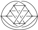
Figure 8. The MMIK graph $G_{S}$.

We remark that among these three families, the only instances of a graph with a degree 2 vertex occur in the family $H_{8}+e$, which also contains no MMIK graphs. This observation suggests the following question.

Question 3.7.

If $G$ has minimal degree $\delta(G)<3$, is it true that $G$’s ancestors and descendants include no MMIK graphs?

Initially, we suspected that such a $G$ has no MMIK cousins at all. However, we discovered that the MMIK graph of size 26, described in Section 4 below, includes graphs of minimal degree two among its cousins. Although we have not completely resolved the question, we have two partial results.

Theorem 3.8.

If $\delta(G)<3$ and $H$ is a descendant of $G$, then $H$ is not MMIK.

Proof.

Since $\delta(G)$ is non-increasing under the $\nabla\mathrm{Y}$ move, $\delta(H)\leq\delta(G)<3$ and $H$ is not MMIK by Lemma 3.3. ∎

As defined in [GMN] a graph has a $\bar{Y}$ if there is a degree 3 vertex that is also part of a $3$-cycle. A $\mathrm{Y}\nabla$ move at such a vertex would result in doubled edges.

Lemma 3.9.

A graph with a $\bar{Y}$ is not MMIK.

Proof.

Let $G$ have a vertex $v$ with $N(v)=\{a,b,c\}$ and $ab\in E(G)$. We can assume $G$ is IK. Make a $\nabla\mathrm{Y}$ move on triangle $v,a,b$ to obtain the graph $H$. By Lemma 3.4 $H$ is IK, as is the homeomorphic graph $H^{\prime}$ obtained by contracting an edge at the degree 2 vertex $c$. But $H^{\prime}=G-ab$ is obtained by deleting an edge $ab$ from $G$. Since $G$ has a proper subgraph $H^{\prime}$ that is IK, $G$ is not MMIK. ∎

Theorem 3.10.

If $G$ has a child $H$ with $\delta(H)<3$, then $G$ is not MMIK.

Proof.

By Lemma 3.3, we can assume $G$ is IK with $\delta(G)=3$. It follows that $G$ has a $\bar{Y}$ and is not MMIK by the previous lemma. ∎

Suppose $G$ is a size 23 MMIK expansion of one of the six nIK Heawood family graphs. We will argue that $G$ must be an expansion of one of the graphs in the three families, $H_{8}+e$, $E_{9}+e$, and $H_{9}+e$. However, as a MMIK graph, $G$ can have no size 22 IK minor. Therefore, $G$ must be an expansion of one of the 29 nIK graphs in the $H_{8}+e$ family.

There are two ways to form a size 22 expansion of one of the six nIK graphs, either add an edge or split a vertex. We now show that if $H$ is in the Heawood family, then $H+e$ is in one of the three families, $H_{8}+e$, $E_{9}+e$, and $H_{9}+e$. We begin with a general observation about how adding an edge to a graph $G$ interacts with the graph’s family.

Theorem 3.11.

If $G$ is a parent of $H$, then every $G+e$ has a cousin that is an $H+e$.

Proof.

Let $H$ be obtained by a $\nabla\mathrm{Y}$ move that replaces the triangle $abc$ in $G$ with three edges on the new vertex $v$. That is, $V(H)=V(G)\cup\{v\}$. Form $G+e$ by adding the edge $e=xy$. Since $V(H)=V(G)\cup\{v\}$, then $x,y\in V(H)$ and the graph $H+e$ is a cousin of $G+e$ by a $\nabla\mathrm{Y}$ move on the triangle $abc$. ∎

Corollary 3.12.

If $G$ is an ancestor of $H$, then every $G+e$ has a cousin that is an $H+e$.

Since every graph in the Heawood family is an ancestor of either the Heawood graph (called $C_{14}$ in [HNTY]) or the graph $H_{12}$, it will be important to understand the graphs that result from adding an edge to these two graphs.

Theorem 3.13.

Let $H$ be the Heawood graph. Up to isomorphism, there are two $H+e$ graphs. One is in the $H_{8}+e$ family, the other in the $E_{9}+e$ family.

Proof.

The diameter of the Heawood graph is three. Up to isomorphism, we can either add an edge between vertices of distance two or three. If we add an edge between vertices of distance two, the result is a graph in the $H_{8}+e$ family. If the distance is three, we are adding an edge between the different parts and the result is a bipartite graph of size 22. As shown in [KMO], this means it is cousin 89 of the $E_{9}+e$ family. ∎

Theorem 3.14.

Let $G$ be formed by adding an edge to $H_{12}$. Then $G$ is in the $H_{8}+e$, $E_{9}+e$, or $H_{9}+e$ family.

Proof.

We remark that $H_{12}$ consists of six degree 4 vertices and six degree 3 vertices. Moreover, five of the degree 3 vertices are created by $\nabla\mathrm{Y}$ moves in the process of obtaining $H_{12}$ from $K_{7}$. Let $a_{i}$ ($i=1\ldots 5$) denote those five degree 3 vertices. Further assume that $b_{1}$ is the remaining degree 3 vertex and $b_{2}$, $b_{3}$, $b_{4}$, $b_{5}$, $b_{6}$ and $b_{7}$ are the remaining degree 4 vertices. Then the $b_{j}$ vertices correspond to vertices of $K_{7}$ before applying the $\nabla\mathrm{Y}$ moves.

First suppose that $G$ is obtained from $H_{12}$ by adding an edge which connects two $b_{j}$ vertices. Since these seven vertices are the vertices of $K_{7}$ before using $\nabla\mathrm{Y}$ moves, there is exactly one vertex among the $a_{i}$, say $a_{1}$, that is adjacent to the two endpoints of the added edge. Let $G^{\prime}$ be the graph obtained from $G$ by applying $\mathrm{Y}\nabla$ moves at $a_{2}$, $a_{3}$, $a_{4}$ and $a_{5}$. Then $G^{\prime}$ is isomorphic to $H_{8}+e$. Therefore $G$ is in the $H_{8}+e$ family.

Next suppose that $G$ is obtained from $H_{12}$ by adding an edge which connects two $a_{i}$ vertices. Let $a_{1}$ and $a_{2}$ be the endpoints of the added edge. We assume that $G^{\prime}$ is obtained from $G$ by using $\mathrm{Y}\nabla$ moves at $a_{3}$, $a_{4}$ and $a_{5}$. Then there are two cases: either $G^{\prime}$ is obtained from $H_{9}$ or $F_{9}$ by adding an edge which connects two degree 3 vertices. In the first case, $G^{\prime}$ is isomorphic to $H_{9}+e$. Thus $G$ is in the $H_{9}+e$ family. In the second case, $G^{\prime}$ is in the $H_{8}+e$ or $E_{9}+e$ family by Corollary 3.12 and Theorem 3.13. Thus $G$ is in the $H_{8}+e$ or $E_{9}+e$ family.

Finally suppose that $G$ is obtained from $H_{12}$ by adding an edge which connects an $a_{i}$ vertex and a $b_{j}$ vertex. Let $a_{1}$ be a vertex of the added edge. We assume that $G^{\prime}$ is the graph obtained from $G$ by using $\mathrm{Y}\nabla$ moves at $a_{2}$, $a_{3}$, $a_{4}$ and $a_{5}$. Since $G^{\prime}$ is obtained from $H_{8}$ by adding an edge, $G^{\prime}$ is in the $H_{8}+e$ or $E_{9}+e$ family by Corollary 3.12 and Theorem 3.13. Therefore $G$ is in the $H_{8}+e$ or $E_{9}+e$ family. ∎

Corollary 3.15.

If $H$ is in the Heawood family, then $H+e$ is in the $H_{8}+e$, $E_{9}+e$, or $H_{9}+e$ family.

Proof.

The graph $H$ is either an ancestor of the Heawood graph or $H_{12}$. Apply Corollary 3.12 and Theorems 3.13 and 3.14. ∎

Corollary 3.16.

If $H$ is in the Heawood family and $H+e$ is nIK, then $H+e$ is one of the 29 nIK graphs in the $H_{8}+e$ family

Lemma 3.17.

Let $H$ be a nIK Heawood family graph and $G$ be an expansion obtained by splitting a vertex of $H$. Then either $G$ has a vertex of degree at most two, or else it is in the $H_{8}+e$, $E_{9}+e$, or $H_{9}+e$ family.

Proof.

Note that $\Delta(H)\leq 5$. If $G$ has no vertex of degree at most two, then the vertex split produces a vertex of degree three. A $\mathrm{Y}\nabla$ move on the degree three vertex produces $G^{\prime}$ which is of the form $H+e$. ∎

Corollary 3.18.

Suppose $G$ is nIK and a size 22 expansion of a nIK Heawood family graph. Then either $G$ has a vertex of degree at most two or $G$ is in the $H_{8}+e$ family.

Theorem 3.19.

Let $G$ be size 23 MMIK with a minor that is a nIK Heawood family graph. Then $G$ is an expansion of one of the 29 nIK graphs in the $H_{8}+e$ family.

Proof.

There must be a size 22 graph $G^{\prime}$ intermediate to $G$ and the Heawood family graph $H$. That is, $G$ is an expansion of $G^{\prime}$, which is an expansion of $H$. By Corollary 3.18, we can assume $G^{\prime}$ has a vertex $v$ of degree at most two.

By Lemma 3.3, a MMIK graph has minimal degree, $\delta(G)\geq 3$. Since $G^{\prime}$ expands to $G$ by adding an edge or splitting a vertex, we conclude $v$ has degree two exactly and $G$ is $G^{\prime}$ with an edge added at $v$. Since $\delta(H)\geq 3$, this means $G^{\prime}$ is obtained from $H$ by a vertex split.

In $G^{\prime}$, let $N(v)=\{a,b\}$ and let $cv$ be the edge added to form $G$. Then $H=G^{\prime}/av$ and we recognize $H+ac$ as a minor of $G$. We are assuming $G$ is MMIK, so $H+ac$ is nIK and, by Corollary 3.16, one of the 29 nIK graphs in the $H_{8}+e$ family. Thus, $G$ is an expansion of $H+ac$, which is one of these 29 graphs, as required. ∎

It remains to study the expansions of the 29 nIK graphs in the $H_{8}+e$ family. We will give an overview of the argument, leaving many of the details to the appendix.

The size 23 expansions of the 29 size 22 nIK graphs fall into one of eight families, which we identify by the number of graphs in the family: $\mathcal{F}_{9}$, $\mathcal{F}_{55}$ $\mathcal{F}_{174}$, $\mathcal{F}_{183}$, $\mathcal{F}_{547}$, $\mathcal{F}_{668}$, $\mathcal{F}_{1229}$, and $\mathcal{F}_{1293}$. We list the graphs in each family in the appendix.

Theorem 3.20.

If $G$ is a size 23 MMIK expansion of a nIK Heawood family graph, then $G$ is in one of the eight families, $\mathcal{F}_{9}$, $\mathcal{F}_{55}$ $\mathcal{F}_{174}$, $\mathcal{F}_{183}$, $\mathcal{F}_{547}$, $\mathcal{F}_{668}$, $\mathcal{F}_{1229}$, and $\mathcal{F}_{1293}$.

Proof.

By Theorem 3.19, $G$ is an expansion of $G^{\prime}$, which is one of the 29 nIK graphs in the $H_{8}+e$ family. As we have seen, these 29 graphs are ancestors of the six graphs $T_{1},\ldots,T_{6}$. By Corollary 3.12, we can find the $G^{\prime}+e$ graphs by looking at the six graphs. Given the family listings in the appendix, it is straightforward to verify that each $T_{i}+e$ is in one of the eight families. This accounts for the graphs $G$ obtained by adding an edge to one of the 29 nIK graphs in the $H_{8}+e$ family.

If instead $G$ is obtained by splitting a vertex of $G^{\prime}$, we use the strategy of Lemma 3.17. By lemma 3.3, $\delta(G)\geq 3$. Since $\Delta(G^{\prime})\leq 5$, the vertex split must produce a vertex of degree three. Then, a $\mathrm{Y}\nabla$ move on the degree three vertex produces $G^{\prime\prime}$ which is of the form $G^{\prime}+e$. Thus $G$ is a cousin of $G^{\prime}+e$ and must be in one of the eight families. ∎

To complete our argument that there is no size 23 MMIK graph with a nIK Heawood family minor, we argue that there are no MMIK graphs in the eight families $\mathcal{F}_{9},\mathcal{F}_{55},\ldots,\mathcal{F}_{1293}$. In large part our argument is based on two criteria that immediately show a graph $G$ is not MMIK.

1. $\delta(G)<3$, see Lemma 3.3.

2. By deleting an edge, there is a proper minor $G-e$ that is an IK graph in the $H_{8}+e$, $E_{9}+e$, or $H_{9}+e$ families. In this case $G$ is IK, but not MMIK.

By Lemma 3.5, if $G$ has an ancestor that satisfies criterion 2, then $G$ is also not MMIK. By Lemma 3.4, if $G$ has a nIK descendant, then $G$ is also not nIK.

Theorem 3.21.

There is no MMIK graph in the $\mathcal{F}_{9}$ family.

Proof.

Four of the nine graphs satisfy the first criterion, $\delta(G)=2$, and these are not MMIK by Lemma 3.3. The remaining graphs are descendants of a graph $G$ that is IK but not MMIK. Indeed, $G$ satisfies criterion 2: by deleting an edge, we recognize $G-e$ as an IK graph in the $H_{9}+e$ family (see the appendix for details). By Lemma 3.5, $G$ and its descendants are also not MMIK. ∎

Theorem 3.22.

There is no MMIK graph in the $\mathcal{F}_{55}$ family.

Proof.

All graphs in this family have $\delta(G)\geq 3$, so none satisfy the first criterion. All but two of the graphs in this family are not MMIK by the second criterion. The remaining two graphs have a common parent that is IK but not MMIK. By Lemma 3.5, these last two graphs are also not MMIK. See the appendix for details. ∎

We remark that $\mathcal{F}_{55}$ is the only one of the eight families that has no graph with $\delta(G)<3$.

Theorem 3.23.

There is no MMIK graph in the $\mathcal{F}_{174}$ family.

Proof.

All but 51 graphs are not MMIK by the first criterion. Of the remaining graphs, all but 17 are not MMIK by the second criterion. Of these, 11 are descendants of a graph $G$ that is IK but not MMIK by the second criterion. By Lemma 3.5, these 11 are also not MMIK. This leaves six graphs. For these we find two nIK descendants. By Lemma 3.4 the remaining six are also not MMIK. Both descendants have a degree 2 vertex. On contracting an edge of the degree 2 vertex, we obtain a homeomorphic graph that is one of the 29 nIK graphs in the $H_{8}+e$ family. ∎

Theorem 3.24.

There is no MMIK graph in the $\mathcal{F}_{183}$ family.

Proof.

All graphs in this family have a vertex of degree two or less and are not MMIK by the first criterion. ∎

Theorem 3.25.

There is no MMIK graph in the $\mathcal{F}_{547}$ family.

Proof.

All but 229 of the graphs in the family are not MMIK by criterion one. Of those, all but 52 are not MMIK by criterion two. Of those, 25 are ancestors of one of the graphs meeting criterion two and are not MMIK by Lemma 3.5. For the remaining 27 graphs, all but five have a nIK descendant and are not IK by Lemma 3.4. For the remaining five, three are ancestors of one of the five. In Figure 9 we give knotless embeddings of the other two graphs. Using Lemma 3.4, all five graphs are nIK, hence not MMIK. ∎

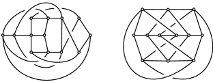
Figure 9. Knotless embeddings of two graphs in $\mathcal{F}_{547}$.

Theorem 3.26.

There is no MMIK graph in the $\mathcal{F}_{668}$ family.

Proof.

All but 283 of the graphs in the family are not MMIK by criterion one. Of those, all but 56 are not MMIK by criterion two. Of those, 23 are ancestors of one of the graphs meeting criterion two and are not MMIK by Lemma 3.5. For the remaining 33 graphs all but three have a nIK descendant and are not IK by Lemma 3.4. Of the remaining three, two are ancestors of the third. Figure 10 is a knotless embedding of the common descendant. By Lemma 3.4 all three of these graphs are nIK, hence not MMIK. ∎

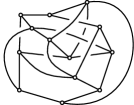
Figure 10. Knotless embedding of a graph in $\mathcal{F}_{668}$.

Theorem 3.27.

There is no MMIK graph in the $\mathcal{F}_{1229}$ family.

Proof.

There are 268 graphs in the family that are not MMIK by criterion one. Of the remaining 961 graphs, all but 140 are not MMIK by criterion two. Of those, all but three are ancestors of one of the graphs meeting criterion two and are not MMIK by Lemma 3.5. The remaining three graphs have an IK minor by contracting an edge and are, therefore, not MMIK. ∎

Theorem 3.28.

There is no MMIK graph in the $\mathcal{F}_{1293}$ family.

Proof.

There are 570 graphs in the family that are not MMIK by criterion one. Of the remaining 723 graphs, all but 99 are not MMIK by criterion two. Of those, all but 12 are ancestors of one of the graphs meeting criterion two and are not MMIK by Lemma 3.5. The remaining 12 graphs have an IK minor by contracing an edge and are, therefore, not MMIK. ∎

3.3. Expansions of the size 22 graphs $H_{1}$ and $H_{2}$

We have argued that a size 23 MMIK graph must have a minor that is either one of six nIK graphs in the Heawood family, or else one of two $(11,22)$ graphs that we call $H_{1}$: J?B@xzoyEo? and $H_{2}$: J?bFF‘wN?{? (see Figure 2). We treated expansions of the Heawood family graphs in the previous subsection. In this subsection we show that $G_{1}$, $G_{2}$, and $G_{3}$ are the only size 23 MMIK expansions of $H_{1}$ and $H_{2}$.

By Lemma 3.3, if a vertex split of $H_{1}$ results in a vertex of degree less than three, the resulting graph is not MMIK. Since $H_{1}$ is $4$-regular, the only other way to make a vertex split produces adjacent degree 3 vertices. Then, a $\mathrm{Y}\nabla$ move on one of the degree three vertices yields an $H_{1}+e$. Thus, a size 23 MMIK expansion of $H_{1}$ must be in the family of a $H_{1}+e$.

Up to isomorphism, there are six $H_{1}+e$ graphs formed by adding an edge to $H_{1}$. These six graphs generate families of size 6, 2, 2, and 1. Three of the six graphs are in the family of size 6 and there is one each in the remaining three families.

All graphs in the family of size six are ancestors of three graphs. In Figure 11 we provide knotless embeddings of those three graphs. By Lemma 3.4, all graphs in this family are nIK, hence not MMIK.

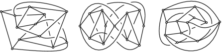
Figure 11. Knotless embeddings of three graphs in the size six family from $H_{1}$.

In a family of two graphs, there is a single $\nabla\mathrm{Y}$ move. In Figure 12 we give knotless embeddings of the children in these two families. By Lemma 3.4, all graphs in these two families are nIK, hence not MMIK.

Figure 12. Knotless embeddings of two graphs in the size two families from $H_{1}$.

The unique graph in the family of size one is $G_{1}$. In subsection 3.1 we show that this graph is MMIK. Using the edge list of $G_{1}$ given above near the beginning of Section 3:

$$[(0,4),(0,5),(0,9),(0,10),(1,4),(1,6),(1,7),(1,10),(2,3),(2,4),(2,5),(2,9),$$

$$(2,10),(3,6),(3,7),(3,8),(4,8),(5,6),(5,7),(5,8),(6,9),(7,9),(8,10)],$$

we recover $H_{1}$ by deleting edge $(2,5)$.

Again, since $H_{2}$ is $4$-regular, MMIK expansions formed by vertex splits (if any) will be in the families of $H_{2}+e$ graphs. Up to isomorphism, there are three $H_{2}+e$ graphs. These produce a family of size four and another of size two.

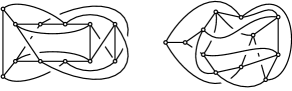
Figure 13. Knotless embeddings of two graphs in the size four family from $H_{2}$.

The family of size four includes two $H_{2}+e$ graphs. All graphs in the family are ancestors of the two graphs that are each shown to have a knotless embedding in Figure 13. By Lemma 3.4, all graphs in this family are nIK, hence not MMIK.

The family of size two consists of the graphs $G_{2}$ and $G_{3}$. In subsection 3.1 we show that these two graphs are MMIK. Using the edge list for $G_{2}$ given above near the beginning of Section 3:

$$[(0,2),(0,4),(0,5),(0,6),(0,7),(1,5),(1,6),(1,7),(1,8),(2,6),(2,7),(2,8),$$

$$(2,9),(3,7),(3,8),(3,9),(3,10),(4,8),(4,9),(4,10),(5,9),(5,10),(6,10)],$$

we recover $H_{2}$ by deleting edge $(0,2)$. As for $G_{3}$:

$$[(0,4),(0,5),(0,7),(0,11),(1,5),(1,6),(1,7),(1,8),(2,7),(2,8),(2,9),(2,11),$$

$$(3,7),(3,8),(3,9),(3,10),(4,8),(4,9),(4,10),(5,9),(5,10),(6,10),(6,11)],$$

contracting edge $(6,11)$ leads back to $H_{2}$.

4. Knotless embedding obstructions of order ten.

In this section, we prove Theorem 1.2: there are exactly 35 obstructions to knotless embedding of order 10. As in the previous section, we refer to knotless embedding obstructions as MMIK graphs. We first describe the 26 graphs given in [FMMNN, MNPP] and then list the 9 new graphs unearthed by our computer search.

4.1. 26 previously known order 10 MMIK graphs.

In [FMMNN], the authors describe 264 MMIK graphs. There are three sporadic graphs (none of order 10), the rest falling into four graph families. Of these, 24 have 10 vertices and they appear in the families as follows.

There are three MMIK graphs of order 10 in the Heawood family [KS, GMN, HNTY]: $H_{10},F_{10},$ and $E_{10}$.

In [GMN], the authors study the other three families. All 56 graphs in the $K_{3,3,1,1}$ family are MMIK. Of these, 11 have order 10: Cousins 4, 5, 6, 7, 22, 25, 26, 27, 28, 48, and 51. There are 33 MMIK graphs in the family of $E_{9}+e$. Of these seven have order 10: Cousins 3, 28, 31, 41, 44, 47, and 50. Finally, the family of $G_{9,28}$ includes 156 MMIK graphs. Of these, there are three of order 10: Cousins 2, 3, and 4.

The other two known MMIK graphs of order 10 are described in [MNPP], one having size 26 and the other size 30. We remark that the family for the graph of size 26 includes both MMIK graphs and graphs with $\delta(G)=2$. However, no ancestor or descendant of a $\delta(G)=2$ graph is MMIK. This is part of our motivation for Question 3.7

4.2. Nine new MMIK graphs of order 10

In this subsection we list the nine additional MMIK graphs that we found after an exhaustive computer search of the 11716571 connected graphs of order 10 conducted in sage [Sg]. In each case, we use the program of [MN] to verify that the graph we found is IK. We use the Mathematica implementation of the program available at Ramin Naimi’s website [N2]. To show that the graph is MMIK, we must in addition verify that each minor formed by deleting or contracting an edge is nIK. Many of these minors are $2$-apex and not IK by Lemma 3.1. There remain 21 minors and below we discuss how we know that those are also nIK.

First we list the nine new MMIK graphs of order 10, including size, graph6 format [Sg], and an edge list.

1. Size: 25; graph6 format: ICrfbp{No

   $$[(0,3),(0,4),(0,5),(0,6),(1,4),(1,5),(1,6),(1,7),(1,8),$$

   $$(2,5),(2,6),(2,7),(2,8),(2,9),(3,6),(3,7),(3,8),$$

   $$(3,9),(4,7),(4,8),(4,9),(5,8),(5,9),(6,9),(7,9)]$$

2. Size: 25; graph6 format: ICrbrrqNg

   $$[(0,3),(0,4),(0,5),(0,8),(1,4),(1,5),(1,6),(1,7),(1,8),$$

   $$(2,5),(2,6),(2,7),(2,8),(2,9),(3,6),(3,7),(3,8),$$

   $$(3,9),(4,6),(4,7),(4,9),(5,9),(6,8),(6,9),(8,9)]$$

3. Size: 25; graph6 format: ICrbrriVg

   $$[(0,3),(0,4),(0,5),(0,8),(1,4),(1,5),(1,6),(1,7),(1,8),$$

   $$(1,9),(2,5),(2,6),(2,7),(2,8),(3,6),(3,7),(3,9),$$

   $$(4,6),(4,7),(4,8),(4,9),(5,9),(6,8),(6,9),(8,9)]$$

4. Size: 25; graph6 format: ICrbrriNW

   $$[(0,3),(0,4),(0,5),(0,8),(1,4),(1,5),(1,6),(1,7),(1,8),$$

   $$(2,5),(2,6),(2,7),(2,8),(2,9),(3,6),(3,7),(3,9),$$

   $$(4,6),(4,7),(4,8),(4,9),(5,9),(6,8),(7,9),(8,9)]$$

5. Size: 27; graph6 format: ICfvRzwfo

   $$[(0,3),(0,4),(0,5),(0,6),(0,8),(0,9),(1,5),(1,6),(1,7),$$

   $$(1,8),(2,5),(2,6),(2,7),(2,8),(3,4),(3,5),(3,7),(3,8),$$

   $$(3,9),(4,6),(4,7),(4,8),(4,9),(5,7),(5,9),(6,9),(7,9)]$$

6. Size: 29; graph6 format: ICfvRr^vo

   $$[(0,3),(0,4),(0,5),(0,6),(0,8),(0,9),(1,5),(1,6),(1,7),(1,8),$$

   $$(1,9),(2,5),(2,6),(2,7),(3,4),(3,5),(3,7),(3,8),(3,9),(4,6),$$

   $$(4,7),(4,8),(4,9),(5,8),(5,9),(6,8),(6,9),(7,8),(7,9)]$$

7. Size: 30; graph6 format: IQjuvrm^o

   $$[(0,2),(0,4),(0,5),(0,6),(0,7),(0,8),(1,3),(1,5),(1,6),(1,7),$$

   $$(1,8),(1,9),(2,4),(2,5),(2,7),(2,8),(2,9),(3,5),(3,6),(3,7),$$

   $$(3,9),(4,6),(4,7),(4,8),(4,9),(5,8),(5,9),(6,8),(6,9),(7,9)]$$

8. Size: 31; graph6 format: IQjur~m^o

   $$[(0,2),(0,4),(0,5),(0,6),(0,8),(1,3),(1,5),(1,6),(1,7),(1,8),(1,9),$$

   $$(2,4),(2,5),(2,7),(2,8),(2,9),(3,5),(3,6),(3,7),(3,9),(4,6),$$

   $$(4,7),(4,8),(4,9),(5,7),(5,8),(5,9),(6,7),(6,8),(6,9),(7,9)]$$

9. Size: 32; graph6 format: IEznfvm|o

   $$[(0,3),(0,4),(0,5),(0,6),(0,7),(0,8),(0,9),(1,3),(1,4),(1,5),(1,6),$$

   $$(1,7),(1,8),(1,9),(2,4),(2,5),(2,6),(2,7),(2,8),(2,9),(3,6),(3,7),$$

   $$(3,9),(4,5),(4,7),(4,8),(5,8),(5,9),(6,7),(6,8),(6,9),(7,9)]$$

To complete our argument, it remains to argue that the 21 non 2-apex minors are nIK. Each of these minors is formed by deleting or contracting an edge in one of the nine graphs just listed. Of these minors, 19 have a 2-apex descendant and are nIK by Lemmas 3.1 and 3.4. In Figure 14 we give knotless embeddings of the remaining two minors showing that they are also nIK.

Figure 14. Knotless embeddings of two order 10 graphs.

5. Acknowledgements

We thank Ramin Naimi for use of his programs which were essential for this project.

References

- [A] D. Archdeacon. A Kuratowski theorem for the projective plane. J. Graph Theory 5 (1981), 243–246.
- [ABDHS] D. Archdeacon, C.P. Bonnington, N. Dean, N. Hartsfield, and K. Scott. Obstruction sets for outer-cylindrical graphs. J. Graph Theory 38 (2001), 42–64.
- [AHLM] D. Archdeacon, N. Hartsfield, C. Little, and B. Mohar. Obstruction sets for outer-projective-planar graphs Ars Combin. 49 (1998), 113–127.
- [BM] J. Barsotti and T.W. Mattman. Graphs on 21 edges that are not 2-apex. Involve 9 (2016), 591–621.
- [BBFFHL] P. Blain, G. Bowlin, T. Fleming, J. Foisy, J. Hendricks, and J. Lacombe. Some results on intrinsically knotted graphs. J. Knot Theory Ramifications 16 (2007), 749–760.
- [BDLST] A. Brouwer, R. Davis, A. Larkin, D. Studenmund, and C. Tucker. Intrinsically 3-Linked Graphs and Other Aspects of Embeddings. Rose-Hulman Undergraduate Mathematics Journal, 8(2) (2007), https://scholar.rose-hulman.edu/rhumj/vol8/iss2/2/ .
- [CMOPRW] J. Campbell, T.W. Mattman, R. Ottman, J. Pyzer, M. Rodrigues, and S. Williams. Intrinsic knotting and linking of almost complete graphs. Kobe J. Math. 25 (2008), 39–58.
- [CG] J. Conway and C.McA. Gordon. Knots and links in spatial graphs. J. Graph Theory 7 (1983), 445–453.
- [DD] G. Ding and S. Dziobiak. Excluded-minor characterization of apex-outerplanar graphs. Graphs Combin. 32 (2016), 583–627.
- [F] J. Foisy. Intrinsically knotted graphs. J. Graph Theory 39 (2002), no. 3, 178–187.
- [FMMNN] E. Flapan, B. Mellor, T.W. Mattman, R. Naimi, and R. Nikkuni. Recent developments in spatial graph theory. Knots, links, spatial graphs, and algebraic invariants, 81–102, Contemp. Math., 689, Amer. Math. Soc., Providence, RI, 2017.
- [GHW] H. Glover, J. Huneke, and C.S. Wang. 103 graphs that are irreducible for the projective plane. J. Combin. Theory Ser. B 27 (1979), 332–370.
- [GMN] N. Goldberg, T.W. Mattman, and R. Naimi. Many, many more intrinsically knotted graphs. Algebr. Geom. Topol. 14 (2014), no. 3, 1801–1823.
- [HNTY] R. Hanaki, R. Nikkuni, K. Taniyama, and A. Yamazaki. On intrinsically knotted or completely 3-linked graphs. Pacific J. Math. 252 (2011), 407–425.
- [JK] A. Jobson and A. Kézdy All minor-minimal apex obstructions with connectivity two. Electron. J. Combin. 28 (2021), Paper No. 1.23, 58 pp.
- [KMO] H. Kim, T.W. Mattman, and S. Oh. Bipartite intrinsically knotted graphs with 22 edges. J. Graph Theory 85 (2017), 568–584.
- [KS] T. Kohara and S. Suzuki. Some remarks on knots and links in spatial graphs. Knots 90 (Osaka, 1990), 435–445, de Gruyter, Berlin, 1992.
- [K] K. Kuratowski. Sur le problème des courbes gauches en topologie. Fund. Math. 15 (1930), 271–283.
- [LMMPRTW] M. Lipton, E. Mackall, T.W. Mattman, M. Pierce, S. Robinson, J. Thomas, and I. Weinschelbaum. Six variations on a theme: almost planar graphs. Involve 11 (2018), 413–448.
- [M] T.W. Mattman. Graphs of 20 edges are 2-apex, hence unknotted. Algebr. Geom. Topol. 11 (2011), 691–718.
- [MNPP] T.W. Mattman, R. Naimi, A. Pavelescu, and E. Pavelescu. Intrinsically knotted graphs with linklessly embeddable simple minors. (preprint) arXiv:2111.08859.
- [MMR] T.W. Mattman, C. Morris, and J. Ryker. Order nine MMIK graphs. Knots, links, spatial graphs, and algebraic invariants, 103–124, Contemp. Math., 689, Amer. Math. Soc., Providence, RI, 2017.
- [MP] T.W. Mattman and M. Pierce. The and families and obstructions to -apex. Knots, links, spatial graphs, and algebraic invariants, 137–158, Contemp. Math., 689, Amer. Math. Soc., Providence, RI, 2017.
- [MN] J. Miller and R. Naimi. An algorithm for detecting intrinsically knotted graphs. Exp. Math. 23 (2014), 6–12.
- [MT] B. Mohar and C. Thomassen. Graphs on surfaces. Johns Hopkins Studies in the Mathematical Sciences. Johns Hopkins University Press, Baltimore, MD, 2001.
- [MW] W. Myrvold and J. Woodcock. A large set of torus obstructions and how they were discovered. Electron. J. Combin. 25 (2018), Paper No. 1.16, 17 pp.
- [N1] R. Naimi. Private communication.
- [N2] R. Naimi. https://sites.oxy.edu/rnaimi/ .
- [OT] M. Ozawa and Y. Tsutsumi. Primitive spatial graphs and graph minors. Rev. Mat. Complut. 20 (2007), 391–406.
- [P] M. Pierce Searching for and classifying the finite set of minor-minimal non-apex graphs, CSU, Chico Honor’s Thesis., (2014). Available at http://tmattman.yourweb.csuchico.edu/ .
- [RS] N. Robertson and P.D. Seymour. Graph minors. XX. Wagner’s conjecture. J. Combin. Theory Ser. B 92 (2004), 325–357.
- [RST] N. Robertson, P. Seymour, and R. Thomas. Sachs’ linkless embedding conjecture. J. Combin. Theory Ser. B 64 (1995), 185–227.
- [Sc] H. Sachs. On spatial representations of finite graphs. Finite and infinite sets, Vol. I, II (Eger, 1981), 649–662, Colloq. Math. Soc. János Bolyai, 37, North-Holland, Amsterdam, 1984.
- [Sg] SageMath, the Sage Mathematics Software System (Version 9.6), The Sage Developers, 2022, https://www.sagemath.org .
- [TY] K. Taniyama, A. Yasuhara. Realization of knots and links in a spatial graph. Topology Appl. 112 (2001), 87–109.
- [W] Wagner, K.: Über eine Eigenschaft der ebenen Komplexe. Math. Ann. 114 (1937), 570–590.