Learning to Find Proofs and Theorems by
Learning to Refine Search Strategies
The Case of Loop Invariant Synthesis

Abstract

We propose a new approach to automated theorem proving where an AlphaZero-style agent is self-training to refine a generic high-level expert strategy expressed as a nondeterministic program. An analogous teacher agent is self-training to generate tasks of suitable relevance and difficulty for the learner. This allows leveraging minimal amounts of domain knowledge to tackle problems for which training data is unavailable or hard to synthesize. As a specific illustration, we consider loop invariant synthesis for imperative programs and use neural networks to refine both the teacher and solver strategies.

1 Introduction

Augmenting tactic-based interactive theorem provers with neural guidance has been the focus of increased attention in recent years [1, 2, 3, 4, 5]. The dominant approach uses imitation learning on corpora of formalized mathematics. However, despite recent efforts involving self-supervised pre-training [5] or data-augmentation [6], this approach is limited by the conspicuous scarcity of human-produced training data. An alternative approach inspired by the success of AlphaZero [7] is to use reinforcement learning and let an agent self-train to interact with a theorem prover via trial and error [8, 9]. However, previous attempts of doing so have been hampered by two fundamental issues:

• First, existing tactic-based theorem provers offer infinite action spaces not amenable to random exploration. Also, they are optimized for formalizing the outcome of human insights concisely but often fail to define a tractable search space for deriving those insights in the first place [10]. For example, using tactics effectively often requires providing insights in advance that are more easily found later in the search process (e.g. constructing a term to instantiate an existential quantifier [11]). More generally, most of the human process of discovering proofs, which involves trial and error, sketching, and abductive reasoning is not captured by standard prover tactics and so we can hardly expect a reinforcement learning agent to learn this process through sheer interaction with a tactic-based prover.

• Second, although reinforcement learning alleviates the need for human proofs during training, the agent must still be provided learning tasks of suitable relevance, diversity, difficulty, and generalizability in the form of theorem statements to be proved. This is in contrast with applications of AlphaZero in board games, where the symmetric nature of games such as Chess or Go enables leveraging symmetric self-play as an infinite source of training tasks.

In this paper, we suggest a novel approach to learning automated theorem proving that does not rely on human-provided proofs and theorems. Instead, a teacher agent is trained to generate interesting and relevant tasks while a solver agent is co-trained to solve them. Our core insight is that both agents can be implemented by using reinforcement learning to refine high-level search strategies [10] written by experts in the form of nondeterministic programs. Our paper also defines novel design principles and language constructs for expressing such strategies. These include conditional generative strategies as a template for implementing teachers, abductive reasoning as a design principle that is made scalable by self-learned guidance, and strategy events as an abstraction that enables easier reward engineering and better sample-efficiency. This paper introduces our new framework and also evaluates it in a well-contained yet challenging setting, namely the automatic verification of imperative programs with loops. We frame our contributions in a way to emphasize general applicability. An empirical evaluation in other application domains is left to future work.

2 Approach

2.1 Background: Verifying Imperative Programs with Loops

Suppose we are given a program such as the one in Figure 1 and we want to prove that the final assertion always holds. The way to proceed is to find a predicate called a loop invariant with the following properties: i) it is true before the loop is entered, ii) it is preserved by the loop body when the loop guard holds and iii) it implies the final assertion when the loop guard does not hold. By “preserved”, we mean that if the invariant is true before executing the loop body then it is also true afterwards. Finding loop invariants is the most crucial aspect of program verification [12, 13] and still resists automation [14].

⬇

assume x >= 1;

y = 0;

while (y < 1000) {

x = x + y;

y = y + 1;

}

assert x >= y;

A desirable invariant is a formula $I[x,y]$ such that:

$$\forall x,y\ \begin{cases}x\geq 1\,\wedge\,y=0\ \rightarrow\ I[x,y]&\ \text{(holds initially)}\\ y<1000\,\wedge\,I[x,y]\ \rightarrow\ I[x+y,y+1]&\ \text{(preserved)}\\ y\geq 1000\,\wedge\,I[x,y]\ \rightarrow\ x\geq y&\ \text{(implies post)}\end{cases}$$

Such an invariant is $I[x,y]:=(x\geq y\,\wedge\,x\geq 1\,\wedge\,y\geq 0)$

 

Figure 1: An example program and an associated loop invariant

Despite the difficulty of automatically synthesizing loop invariants, humans do so routinely using well-understood search strategies. For example, in the case of the example in Figure 1, one would first try to prove the postcondition $x\geq y$ itself as an invariant and then note that it is not preserved by the loop body as the following implication does not hold: $y<1000\,\wedge\,x\geq y\centernot\ \rightarrow\ x+y\geq y+1$. However, simplifying the right-hand side, we see that the proof works if we can show $x\geq 1$ to be an invariant itself. Using a similar form of abductive reasoning, we find that this in turn requires $y\geq 0$ to be an invariant and we end up proposing $x\geq y\wedge x\geq 1\wedge y\geq 0$ as a loop invariant.

2.2 Expressing Search Strategies as Nondeterministic Programs

The search strategy we followed for the example above can be formalized as a nondeterministic program, which is shown in Figure 2. As a nondeterministic program, it features a choose operator that takes a list of objects as an input and selects one of them nondeterministically. A nondeterministic program can be refined into a deterministic one by providing an external oracle to implement the choose operator. It also defines a search tree that can be explored with or without a guiding heuristic. In this work, we use neural networks to implement such oracles and guiding heuristics.

⬇

1def solver(

2 init: Formula, guard: Formula,

3 body: Program, post: Formula) -> Formula:

4

5 def prove_inv(inv: Formula) -> List[Formula]:

6 assert valid(Implies(init, inv))

7 inductive = Implies(And(guard, inv), wlp(body, inv))

8 match abduct(inductive):

9 case Valid:

10 return [inv]

11 case [*suggestions]:

12 aux = choose(suggestions)

13 return [inv] + prove_inv(aux)

14

15 inv_cand = choose(abduct(Implies(Not(guard), post)))

16 inv_conjuncts = prove_inv(inv_cand)

17 reward(max(-1, -0.2 * len(inv_conjuncts))

18 return And(*inv_conjuncts)

Figure 2: A simple strategy for finding loop invariants, described in Python-like pseudocode syntax. In this strategy, an initial invariant candidate is selected nondeterministically that implies the postcondition (line 15). One ensures that this candidate holds initially (line 6), without which the strategy fails immediately. Then, one attempts to prove that it is preserved by the loop body (lines 7 and 8, where wlp denotes Hoare’s weakest liberal precondition operator [15]). If the candidate is not preserved, the abduct function suggests a list of assumptions that make it so. One then uses the choose operator to nondeterministically select one of them, which we try and prove invariant recursively (line 13). Because the number of abduction candidates to choose from can be large, successfully using such a strategy depends on having an effective oracle to guide search. To provide sufficient context to such an oracle, calls to choose must provide some extra information that is omitted here for brevity. In this case, we would pass a special token to indicate the call site, the program being analyzed and the value of inv in the case of line 12. See Appendix A for more details and for a full listing of the invariant synthesis strategy that we use in our experiments.

In addition, a key aspect of this strategy is to infer missing assumptions under which a currently failing proof obligation would hold. This form of reasoning is called abductive reasoning and it is fundamental in the way humans search for proofs [16, 17]. It is implemented in a separate abduct procedure that takes a formula as an input and returns either Valid or a list of abduction candidates. For example, the abduct procedure fails to prove the implication $x\geq 0\rightarrow x+y\geq 1$ but may suggest $x+y\geq 1$, $x<0$ and $y\geq 1$ as possible missing assumptions. The use of abductive reasoning for theorem proving and loop invariant synthesis specifically has been proposed in the past [18, 19]. However, abduction procedures are hard to implement [20] and typically only available for specific decidable theories. Also, using them in proof search tends to scale poorly in the absence of good heuristics to rank and filter abduction candidates. Our proposed framework makes abductive reasoning practical by addressing both issues: it allows leveraging self-learned guidance to select abduction candidates and it allows implementing abduction procedures as nondeterministic programs that are amenable to learning themselves.

Another notable feature of the strategy in Figure 2 is the use of the reward operator on line 17 to incentivize finding short invariants (short proofs are desirable in general as they tend to be easier to check, interpret and generalize). The reward operator can be used multiple times and at any point of the strategy execution. An implicit reward of 1 or -1 is emitted when the strategy successfully returns or fails respectively. An optimal execution of a nondeterministic strategy is one that maximizes the cumulative amount of collected rewards. In this example, we bound the maximal invariant size penalty in such a way to ensure that finding a proof is always rewarded more than failing at doing so.

As argued by Selsam [10], defining search strategies as nondeterministic programs provides a natural and flexible way for experts to leverage domain-specific knowledge while outsourcing difficult proof decisions to search algorithms and learned heuristics. This paradigm differs from the standard paradigm of tactic-based theorem provers in which an external entity must orchestrate stateless tactics that do not call for any form of interactive guidance internally. In contrast, the nondeterministic programming approach inverts control and has strategies call external oracles rather than the other way around, which allows for a much tighter control of the resulting search space.

2.3 Refining Nondeterministic Strategies with Reinforcement Learning

A nondeterministic program induces a (deterministic) Markov Decision Process (MDP) where intermediate states are choice points and final states are either success states (the program returns successfully) or failure states (an assertion is violated or choose is called on an empty list of choices). Standard search algorithms can be used to navigate this MDP but doing so in an efficient and scalable way requires strong heuristics for guiding search.

In this work, we propose to learn such heuristics in a self-supervised fashion using the AlphaZero algorithm [7, 21]. In AlphaZero, a neural network is trained to map any state to a probability distribution over available actions along with a value estimate (i.e. an estimate of the expected sum of future rewards). The neural network alone can be used as a policy for navigating the MDP. However, a stronger policy results from combining the network with a tree search algorithm such as Monte-Carlo Tree Search (MCTS) [22]. The key insight underlying AlphaZero is that the network can be trained via an iterative improvement process where it is successively i) used as an MCTS heuristic to try and solve problems and then ii) updated using gradient descent so as to better predict the outcome of each attempt along with the action selected by MCTS on all states encountered along the way. More details on AlphaZero can be found in the literature [7].

Using AlphaZero, we can refine nondeterministic proof search strategies without external proof examples to learn from. However, AlphaZero must still be provided with a set of training problems to be solved. Training problems should be diverse, relevant and numerous enough to allow proper generalization. They should also be of varied difficulty to allow for learning to bootstrap.

2.4 Generating Training Problems with Conditional Generative Strategies

In theorem proving, high-quality training problems produced by humans are often not available in quantities even remotely matching the needs of reinforcement learning to properly generalize across problem instances. A possible solution is to use procedural generation techniques to assemble large datasets of synthetic problems. This works well in some specific areas [23] and particularly for problems that can be framed as inverse problems such as symbolic integration [24]. In other areas, generating interesting problems is as hard as solving existing ones, possibly harder.

This is the case in particular with the problem of loop invariant synthesis. Here, a natural idea for generating problem instances would be to use a probabilistic grammar for repeatedly sampling triples consisting of a program, a loop invariant and an assertion and then reject all triples in which the properties defining valid invariants do not hold. Unfortunately, not only would doing so naively lead to a very high rejection rate, but the resulting dataset would be heavily biased towards trivial samples that are hardest to reject (e.g. programs where the final assertion is the negation of the loop guard and where the invariant does not even matter). In contrast, many classes of interesting problems from standard human-written benchmarks would only be sampled with an infinitesimal probability.

In this work, we propose to generate problems using the same methodology we use to solve them: by leveraging reinforcement learning to refine nondeterministic search strategies.

Specifically, experts can define teacher strategies in the form of stochastic and nondeterministic programs, each run of which either fails or successfully returns with a problem instance. Reinforcement learning can then be used to refine such programs with the two objectives of maximizing the diversity and interestingness of generated problems while avoiding rejection. However, these objectives are naturally in tension since an agent may be locally incentivized to avoid generating particular types of problems that are easier to reject. We introduce a design template for a class of strategies that avoid this obstacle. We call such strategies conditional generative strategies.

A conditional generative strategy generates a problem in three steps: i) it samples a set of constraints that define desired features for the generated problem, ii) it nondeterministically generates a problem that respects as many constraints as possible and gets rewarded for doing so and iii) it applies a sequence of random and validity-preserving problem transformations as a way to further increase diversity. We provide a high-level description of a such a teacher strategy for invariant synthesis in Figure 3. The interest of such an architecture is that it enables decoupling the two conflicting objectives of generating valid and diverse problems: diversity is guaranteed by the first and third steps while learning can focus on the second step. This also allows using the exact same learning algorithm for training both teacher and solver agents (AlphaZero in this work).

⬇

1def teacher(rng: RandGen) -> Prog:

2 cs = sample_constrs(rng)

3 p = generate_prog(cs)

4 p = transform(p, rng)

5 p = hide_invariants(p)

6 return p

7

8def generate_prog(cs: Constrs):

9 p = Prog("

10 assume init;

11 while (guard) {

12 invariant inv_lin;

13 invariant inv_aux;

14 invariant inv_main;

15 body;

16 }

17 assert post;")

18 p = refine_guard(p, cs)

⬇

18 p = refine_inv(p, cs)

19 p = refine_body(p, cs)

20 assert valid(inv_preserved(p))

21 p = refine_post(p, cs)

22 assert valid(inv_post(p))

23 p = refine_init(p, cs)

24 assert valid(inv_init(p))

25 nv = num_violations(p, cs)

26 reward(max(-1.5, -0.5 * nv))

27 return p

28

29def transform(p: Prog, rng: RandGen):

30 p = shuffle_formulas(p, rng)

31 p = shuffle_instrs(p, rng)

32 p = add_useless_init(p, rng)

33 p = add_useless_post(p, rng)

34 ...

35 return p

Figure 3: Simplified teacher strategy. Problems are generated by nondeterministically refining the template in lines 10-17 in a way to optimize random constraints (see examples in Table 1). In this template, the invariant is expressed as a conjunction of at most three sub-invariants: inv_lin is a linear equality or inequality, inv_main is a disjunction of atomic formulas (i.e. comparisons) and inv_aux is a conjunction of atomic formulas that can be used in proving inv_main but not post. These three formulas are refined nondeterministically by the call to refine_inv on line 18. After an invariant is chosen, a loop body is also generated nondeterministically (line 19) that preserves the invariant (line 20). Finally, the num_violations function penalizes the presence of useless or redundant problem components. For example, a penalty is applied if inv_main features a disjunct that can be removed without invalidating the problem. Appendix B provides more details on how the refine_* functions can be implemented. The simplest way to do so is to have a grammar and use the choose operator to select rules recursively. However, fancier strategies can easily be implemented in the nondeterministic programming framework. In particular, our implementation uses the abduct procedure introduced in Figure 2 to suggest values for constants and subformulas.

Name	Type	Description
num-inv-main-disjuncts	none|1|2	If an integer $n$, then inv_main is refined with a disjunction of $n$ atomic formulas.
has-conditional	bool	Whether body must include a conditional statement.
loop-guard-useful-for-post	bool	Whether assuming the negation of the loop guard is useful in proving the postcondition post.
body-implies-main-inv	bool	If true, then inv_main always holds after executing body regardless of whether or not it holds before.
eq-only-for-init	bool	Whether or not to use equalities only in init.

Table 1: Examples of teacher constraints. Some descriptions refer to names introduced in Figure 3. The full list of constraints we used in our experiments is available in Appendix B.

2.5 Predicting Events Rather Than Rewards

In the standard AlphaZero setting, the network is trained to predict the value of encountered states, that is the expected sum of future rewards. However, such a number conflates a lot of valuable information. For example, suppose a teacher state is assigned a value of 0. Does 0 mean that the teacher is predicted to either fail or succeed with equal probability or that it will certainly succeed in generating a problem that violates two constraints? And if so, which two?

Although this information is not relevant to MCTS, there are several reasons for having the network predict it anyway. First, doing so can result in an increased sample efficiency by providing the network with more detailed feedback on its mistakes. Such an effect has been previously demonstrated in the KataGo project [25]. Second, it is interesting from an interpretability point of view and makes it easier to diagnose problems and weaknesses in a given network. We found a third reason that is more subtle, which has to do with getting the combined benefits of issuing intermediate and final rewards.

Indeed, in the teacher strategy showed in Figure 3, we only penalize the agent for violating a constraint at the very end. Intuitively, there is a lost opportunity here since many violations could be detected much earlier while the problem is still being refined. Emitting an intermediate reward at this point would certainly improve learning efficiency. However, the same violation can be potentially detected at several different points in time and we must ensure that a reward is only issued the first time. This in turns makes the job of the value prediction network harder since it needs to keep track of whether or not each violation has been penalized already. Encoding this information alone can be costly, and especially so for attention-based network architectures such as transformers with a quadratic inference cost. Having the network predict constraint violations separately offers an elegant way out: all rewards are issued at the end but from the moment a constraint violation is detected, the network’s predicted probability for this violation is overridden to 1 whenever a value estimate is computed.

More formally, we propose to introduce the concept of an event. Strategies can declare an arbitrary number of events $e$ and each one is associated with a reward $r_{e}$ along with a maximal number of occurrences $m_{e}$ ($m_{e}=1$ for constraint violation events) that can be counted towards the final reward. The reward operator introduced in Figure 2 is replaced by an event operator. When a strategy terminates, a reward is issued implicitly with a value of $-1$ in case of a failure and

$$\max\Big{\{}1+\sum_{e}r_{e}\min(n_{e},m_{e}),\ r_{\texttt{min}}\Big{\}}$$

in case of a success. In this expression, $n_{e}$ denotes the number of calls made to $\texttt{event}(e)$ during the whole episode and setting $r_{\texttt{min}}>-1$ guarantees that successes are always rewarded more than failures. Note that it is important not to issue event penalties after a failure. Otherwise, faced with a likely failure, an agent may be incentivized to simply give up and fail immediately to avoid further penalties in search of success. Also, there are two reasons for bounding the maximal number of occurrences of event $e$ that are counted towards the final reward by a constant quantity $m_{e}$. First, this allows having a network with a finite softmax head predict the number of occurrences of $e$ (as we see below). Second, the $m_{e}=1$ case is particularly useful to model events such as constraint violations that can be detected multiple times but should only be penalized once.

In this framework, the value head of the network is tasked with predicting the following probabilities: i) the probability $p_{0}$ of a failure, ii) the probability $p_{1}$ of succeeding with minimal reward $r_{\texttt{min}}$, iii) the probability $p_{2}=1-p_{0}-p_{1}$ of succeeding with a greater reward and iv) the probabilities $p_{e}^{i}$ that $\min(n_{e},m_{e})=i$ for all events $e$ and $0\leq i\leq m_{e}$. A value estimate derives from these probabilities:

$$-p_{0}+p_{1}\cdot r_{\texttt{min}}+p_{2}\cdot\sum_{e}\sum_{i}\hat{p}_{e}^{i}\cdot i\cdot r_{e}$$

where $\hat{p}_{e}^{i}\propto\mathbf{1}{\{n_{e}\leq i\}}\cdot p_{e}^{i}$ is a corrected probability estimate accounting for the number of times $n_{e}$ that $\texttt{event}(e)$ was raised already. In our invariant synthesis experiments, we use events in both the teacher and solver strategies to represent constraint violations $(m_{e}=1)$ and encourage short proofs by penalizing individual proof steps respectively $(m_{e}>1)$.

3 Implementation and Engineering Contributions

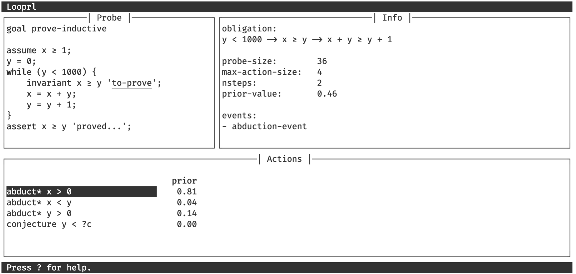
Figure 4: Using the Looprl UI to inspect the solver agent on the problem from Figure 1. Additional commented screenshots are available in Appendix E.

This paper advocates for a hybrid approach to automated theorem proving where human experts from a variety of areas can formalize their knowledge succinctly in the form of nondeterministic proving and teaching strategies. Reinforcement learning is leveraged to fill in the blanks in all inevitable cases where the human intuition escapes formalization.

However, for this vision to be practical, writing strategies and iterating on them must be as frictionless as possible. New tools and abstractions are needed to automate the process of converting nondeterministic programs into reinforcement learning environments, ease debugging and foster code reuse. In this work, we accomplish a crucial step in this direction by introducing the Looprl theorem prover. Looprl consists of the following collection of features:

• A domain specific language for writing strategies embedded in OCaml, with first-class support for neural-guided nondeterministic programming. Strategies are automatically compiled into reinforcement learning environments that can be explored in Python.

• A graphical interface that can be used to interact with strategies manually while inspecting the neural network’s predictions and the behavior of MCTS (see Figure 4).

• A library of utility functions for writing program verification strategies. This library includes an implementation of the abduct function introduced in Figure 2 for integer linear arithmetic (see details in Appendix F).

• A parallel, high-performance implementation of the (Gumbel) AlphaZero algorithm [7, 21] for refining search strategies. Our implementation uses Pytorch [26] and Ray [27]. It provides support for events (see Section 2.5) and unbounded, variable-size action spaces.

The first point on developing a domain-specific language for writing strategies is particularly important and deserves more discussion. In our experience, having such a language is not just a mere matter of convenience but one of feasibility. In fact, we did try to implement an initial version of a teacher strategy for loop invariant synthesis by writing pseudocode on paper and manually compiling it into an MDP implemented in Python. However, doing so resulted in a complexity explosion where any single-line change to the pseudocode could take days of work to implement.

The reason compiling a nondeterministic program into an MDP manually is so tedious is that the whole program state must be made explicit, which includes the program stack. A tempting alternative would be to write nondeterministic code as normal Python code parametrized by an arbitrary choose function. However, this does not allow using tree search on the resulting program since doing so would require cloning the whole execution state of a Python program. Fortunately, there exists a solution to this problem in the field of programming languages using search monads [28, 10] and which essentially enables writing arbitrary nondeterministic code and then reifying it into a search tree that can be manipulated explicitly.

In Looprl, we implement a domain specific language embedded in OCaml for expressing nondeterministic strategies. OCaml is a natural choice because it is fast (about two orders of magnitude faster than Python for symbolic code such as proof inferences) and it has good support for monads and Python interoperability. Our language provides built-in support for the choose and event operators. Also, it defines an intermediate graph-based format for representing data to be sent to neural networks in an architecture-agnostic way. Any piece of information that is passed to the choose operator must be convertible to this format and feature suitable metadata ensuring a seamless integration with the Looprl user interface and debugging tools.

4 Experiments

We tested Looprl on the problem of synthesizing loop invariants for single-loop imperative programs and evaluated it on the standard Code2Inv [29] benchmark. This benchmark contains a set of 132 programs written in C. All programs feature a single loop along with a final assertion to be proven. They feature linear integer arithmetic and sometimes involve conditionals, assumptions and nondeterministic tests (some Code2Inv problems are in Appendix C). Most existing invariant generation tools can only solve a subset of these problems [30]. To the best of our knowledge, only one existing tool can solve them all [31]. However, it does not use learning and relies on specific optimization techniques that are not generalizable beyond the setting of purely numerical programs.

We used Looprl to implement an invariant generation strategy, which we describe in Appendix A. In a nutshell, it generalizes the simple strategy described in Figure 2 by adding features such as the ability to abduct disjunctive invariants or to conjecture invariant templates with placeholder constants to be refined later using abduction. To our surprise and although this generic strategy can be described in only one page of pseudocode, it is sufficient to simply solve every Code2Inv benchmark problem in a few seconds when combined with the vanilla MCTS algorithm [22] (with no learned heuristic).

We therefore evaluate a self-trained solver agent on its ability to solve as many Code2Inv problems as possible without resorting to any search. At every decision point, it greedily takes the highest ranked action according to the network’s policy head and no backtracking is allowed. We argue that such a metric is of particular interest and significance. Indeed, finding an invariant for a single loop is of limited interest of its own. Rather, doing so is typically useful as a subtask in a hierarchy of increasingly complex and relevant problems. The next level of this hierarchy may be to prove a piece of code with nested loops, and then to synthesize a function respecting a specification, which is still several levels away from writing full-fledged software systems. Complex problems cannot be solved if backtracking search is needed at every level of this deep hierarchy.

4.1 Training Protocol

We train a teacher agent and a solver agent in sequence using the (Gumbel) AlphaZero algorithm. Both agents use a similar 1.6M parameters Dynamic Graph Transformer network [32] (see architecture details in Appendix LABEL:ap:network). The teacher agent is trained first for 20 AlphaZero iterations. During each iteration, it goes through 8000 problem generation episodes, using 64 MCTS simulations per step. Then, the network is updated using samples from the $k$ previous iterations with $k$ increasing from 1 to 6 during training. Each iteration simulates 800 additional episodes to generate validation samples that are not used to train the network but to control overfitting via early stopping. After the teacher agent is trained, a dataset of 50K problems is gathered for training the solver, which includes a mix of 40K problems generated during the last five training iterations and 10K new ones that are generated without Gumbel exploration noise [21]. The solver agent is also trained for 20 iterations. During each iteration, it attempts to solve 20K randomly selected problems using 32 MCTS simulations per step. In addition, 5K additional problems are solved to generate validation samples. See Appendix G for a complete list and explanation of all training hyperparameters.

A complete training run takes about 16h on a single machine with a 10-core Intel i9-10900KF processor, 64GB of RAM and a NVIDIA GeForce RTX 3080 GPU.

4.2 Experimental Results

We show training curves for the solver and teacher agents in Figures 6 and 6 respectively. These curves record the evolution of the average reward collected by MCTS combined with the latest network during each iteration. Error intervals are estimated based on two random seeds. Note that the maximum theoretical reward obtainable by the teacher agent is ${<}1$ since problem generation constraints may be sampled that are mutually incompatible, in which case the agent simply does its best to minimize the number of violated constraints. The same holds for the solver agent since all generated invariants are penalized proportionally to their size. The solver agent goes through a more modest reward gain during training (the $y$-axis is rescaled in Figure 6 to emphasize the trend). This is reflective of the fact that most problems generated by the teacher can be solved by MCTS alone and so most of the training concentrates on learning to solve about 10% of hard problems.

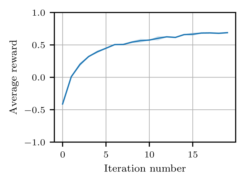
Figure 5: Teacher training curve

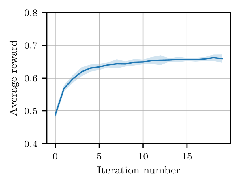
Figure 6: Solver training curve

We show the results of our evaluation on the Code2Inv benchmark in Table 2. Three different agents are compared on the average ratio of benchmark problems for which they can successfully generate an invariant of minimal size without search or backtracking. The first agent is a baseline that simply selects proof actions at random. The second agent is a solver network that was trained using problems generated by an untrained teacher (i.e. using MCTS but no network heuristic). Finally, the third agent is a solver network trained using the full protocol of Section 4.1. These results demonstrate the critical impact of learning for both the teacher and solver agents. Unsurprisingly, an inferior teacher leads to an inferior solver with decreased generalization capabilities.

Policy	% Problems solved
Random	${18.4\ \pm\ 0.0}$
Network (untrained teacher)	${39.7\ \pm\ 1.6}$
Network (trained teacher)	$\mathbf{61.5\ \pm\ 0.4}$

Table 2: Experimental results on the Code2Inv benchmark (using no backtracking search). The score for the Random heuristic is computed as an average across 10K attempts. Standard deviations are computed based on using two different random seeds for the full training experiment.

5 Related Work

Leveraging nondeterministic programming for proof search.   The idea of combining nondeterministic expert strategies with neural oracles was proposed by Selsam [10, 33] as a possible angle for tackling the IMO Grand Challenge [34]. However, how to train such oracles remains an open problem. One proposal [32] is to use supervised learning for training a universal oracle that is conditioned on the description of arbitrary search problems and can therefore use training data from a large number of heterogeneous sources. In contrast, we propose using reinforcement learning with the insight that nondeterministic search strategies can be used to generate problems in addition to solving them.

Learning to generate synthetic theorems.   Procedural generation techniques have been used for producing synthetic theorems [35, 36, 37, 24, 38]. These usually proceed in a backwards fashion by generating random proof trees from a given set of axioms and rules. Wang et al. proposed to use supervised learning to learn how to guide this process towards generating more interesting theorems that are similar to those of a reference dataset [6].

Using reinforcement learning for loop invariant synthesis.   Reinforcement learning has already been applied to the problem of loop invariant synthesis [29, 30], albeit in a very different way. In the aforementioned work (which introduces the Code2Inv benchmark), a separate reinforcement learning agent is trained from scratch on every benchmark problem, using counterexamples from an SMT solver as a training signal. This process takes minutes to hours for each problem to be solved. In contrast, we train a single agent to generalize across problem instances so that new problems can be solved in a matter of milliseconds.

Using reinforcement learning for theorem proving.   The HOList Zero [8] and TacticZero [9] systems use reinforcement learning to learn how to interact with tactic-based theorem provers without relying on human proofs. However, they still rely on large human-produced corpora of formalized mathematical statements to be used as training tasks and are not yet competitive with approaches based on imitation learning. The use of reinforcement learning has also been explored in the context of saturation-based or tableau-based provers for first-order logic [39, 40]. However, learned heuristics in such settings must operate at a very low-level and are subject to a speed-accuracy tradeoff that is unfavorable to deep learning.

6 Conclusions and Future Work

This paper took a bold stride toward the challenge of self-learning automated theorem proving without relying on example theorems and proofs. It advocates a hybrid approach to theorem proving where experts are provided a flexible language to formalize their domain-specific knowledge in the form of generic nondeterministic teacher and solver strategies, leaving blanks to be filled by learning.

We demonstrated our framework by applying it to the problem of loop invariant synthesis. Our agent solves all Code2Inv challenges. More importantly, it learns to solve a majority of problems with no search at all despite never seeing these problems during training.

None of our core contributions, however, are specific to invariant synthesis. These include: i) our key insight that nondeterministic programming and reinforcement learning can be similarly combined to implement solvers and teachers, ii) conditional generative strategiesas a general template to write teachers, iii) abductive reasoningas a design principle that is made scalable by self-learned guidance, iv) strategy eventsfor easier reward engineering and better sample-efficiency, and v) an implementation that establishes engineering foundations for making the whole approach practical.

We see this paper as a first step toward a broader vision where interactive theorem provers allow users to write teacher and solver strategies for domains of mathematics and programming in a modular and distributed fashion. A unique neural network can then be trained as an oracle for all these strategies, allowing better generalization and sample efficiency. However, many challenges lie ahead. In particular, while there is some evidence already [10, 41, 19] that effective solver strategies can be written at scale (interactive theorem provers already allow specifying custom search tactics [42, 43, 44] and we are merely suggesting a generalization of this popular feature), scaling up teacher strategies raises more questions. For example, writing conditional generative strategies can be engineering-intensive since diversity is enforced extrinsically via manually-defined constraints. Future work will explore teachers that also integrate intrinsic reward signals, either via a curiosity mechanism or by having the solver directly reward the teacher for producing problems of suitable novelty and difficulty.

Broader Impact

Automated theorem proving for program verification and program synthesis plays an important role for increasing the safety of critical pieces of software. More automatic theorem provers enable a wider user base to benefit from the advances to their software quality. But automating theorem provers is a highly sophisticated challenge. Learning from succinct expert advice in the form of strategies may be the sweet spot enabling more generic domain-specific automation for theorem provers.

Appendix A Details on the Solver Strategy

In Figure 7, we provide some detailed pseudocode for the solver strategy that we implemented for the purpose of the experiments in Section 4. This strategy is similar to the simple one introduced in Figure 2 but it comes with the following extensions:

• Ability to abduct disjunctive invariants: Imagine a proof obligation fails and the abduct function returns $a_{1},\dots,a_{n}$ as possible missing assumptions. In some cases, none of those can be proved invariant but the disjunction of a subset of them can. This is why the suggest_missing function defined on line 28 is used to build an invariant candidate as a disjunction of at most 3 (atomic) abduction candidates.

• Ability to strengthen abducted invariants: An abducted invariant candidate may have to be strengthened before it can be proved invariant. For example, the abduction engine may suggest $x\neq 0$ as a missing assumption but $x\neq 0$ may not be a valid invariant whereas $x>0$ (or $x<0$) is. The call to strengthen on line 47 is used to optionally and nondeterministically strengthen an invariant candidate. Our current strategy supports two kinds of strengthening: replacing a formula of the form $A\neq B$ by either $A>B$ or $A<B$ or weakening an inequality of the form $A\leq B$ into $A\leq B+c_{?}$ where $c_{?}$ is a nonnegative constant whose exact value is to be determined later (see next point).

• Ability to instantiate constants lazily via abduction: Invariant candidates can feature metavariables that denote unknown constants. The constrs variable defined in line 8 collects global constraints about these metavariables. If a missing assumption is suggested that only features metavariables, then it is added as a constraint rather than as a new invariant candidate (line 42). After an invariant is proved, the metavariables it contains are instantiated using concrete values in a way to satisfy all global constraints (see call to abduct_refinement on line 44). A metavariable that appears in the invariant as an upper bound is instantiated with a value that is as low as possible, whereas a metavariable that appears as a lower bound is instantiated with a value that is as high as possible (this information is contained in the btype variable).

• Ability to conjecture invariant templates: In some cases, abduction alone is not enough to discover a missing invariant. For example, if two disjunctive invariants $I_{1}$ and $I_{2}$ are needed for proving the postcondition, one may have to conjecture the first one and then use abduction to find the other. The strategy in Figure 7 allows conjecturing invariant templates with metavariables to be instantiated via abduction (see previous point). The conjectures function called on line 29 returns three kinds of conjecture candidates: i) conjectures of the form $t\odot c_{?}$ where $\odot\in\{\geq,=\}$ and $t=\sum_{i}a_{i}x_{i}$ is a linear combination of variables that is preserved by the loop body, ii) relaxations of the loop guard (e.g. $x\leq 10+c_{?}$ with $c_{?}>0$ if the loop guard is $x\leq 10$) and iii) initial assumptions that only contain variables that are not modified by the loop body.

The solver strategy also emits two types of events (see Section 2.5) at lines 38 and 36 respectively. Conjecturing events are associated with a reward of $-0.3$ and abduction events are associated with a reward of $-0.2$. Both kinds of events are counted at most four times ($m_{e}=4$) and the minimum total reward delivered in case of a success is $r_{\texttt{min}}=0$.

Hints on how to use our proposed solver strategy to solve Code2Inv benchmark problems are available in Appendix C.

⬇

1def solver(

2 init: Formula,

3 guard: Formula,

4 body: Program,

5 post: Formula) -> List[Formula]:

6

7 invs_proved: List[Formula] = []

8 constrs: List[Formula] = []

9 pending: List[Pending] = []

10

11 def prove_post():

12 pending[-1].status = TO_PROVE

13 to_prove = Implies(

14 constrs + invs_proved + [Not(guard)],

15 post)

16 match abduct(to_prove):

17 case Valid:

18 pending[-1].status = PROVED

19 case [*suggs]:

20 assum = suggest_missing(suggs)

21 closing = implies(assum, to_prove)

22 pending[-1].status = \

23 PROVED_COND if closing

24 else TO_PROVE_NEXT

25 prove_missing(assum, as_inv=True)

26 prove_post()

27

28 def suggest_missing(suggs: List[Formula]):

29 suggs += conjectures(guard, body)

30 num_disjs = choose([1, 2, 3])

31 disjs = []

32 for i in range(num_disjs):

33 d = choose(suggs)

34 disjs.append(d)

35 if is_conjecture(d):

36 event(CONJECTURING_EVENT)

37 else:

38 event(ABDUCTION_EVENT)

39 return Or(*disjs)

40

41 def prove_missing(f: Formula, as_inv: bool):

42 if meta_only(f):

43 constrs.append(f)

44 assert sat(constrs)

45 else:

46 assert as_inv

47 inv, fresh = strengthen(f)

⬇

35 for c, _ in fresh:

36 constrs.append(Ge(Metavar(c), 0))

37 pending.append(

38 Pending(INV, inv, TO_PROVE))

39 prove_init(inv)

40 prove_preserved(inv)

41 invs_proved.append(inv)

42 pending.pop()

43 for c, btype in fresh:

44 cval = abduct_refinement(

45 c, btype, constrs)

46 subst(invs_proved, c, cval)

47 subst(constrs, c, cval)

48

49 def prove_init(inv: Formula):

50 pending[-1].status = TO_PROVE

51 to_prove = Implies(

52 constrs + proved_invs + [init],

53 inv)

54 match abduct(to_prove):

55 case Valid: return

56 case [*suggs]:

57 assum = choose(suggs)

58 prove_missing(assum, False)

59

60 def prove_preserved(inv: Formula):

61 pending[-1].status = TO_PROVE

62 to_prove = Implies(

63 constrs +

64 proved_invs + [guard, inv],

65 loop_body.wlp(inv))

66 match abduct(to_prove):

67 case Valid: return

68 case [*suggs]:

69 suggs = suggest_missing(suggs)

70 closing = implies(assum, to_prove)

71 pending[-1].status = \

72 PROVED_COND if closing

73 else TO_PROVE_NEXT

74 perform(action)

75 prove_inv_inductive(inv)

76

77 pending.append(

78 Pending(POST, post, TO_PROVE))

79 prove_post()

80 pending.pop()

81 return invs_proved

Figure 7: Strategy for the solver agent. The code in gray is only useful for providing the network with contextual information and can be disregarded on first reading. Every call to choose is implicitly passed the program counter along with the value of all global parameters and all variables that are defined in lines 2 to 9. In particular, the pending variable summarizes all information from the program stack that is relevant to the neural network.

Appendix B Details on the Teacher Strategy

The teacher strategy we use for loop invariant generation follows the structure introduced in Figure 3. We provide additional details below:

• Sampling constraints: The full list of available constraints is available in Table 3. Values are sampled mostly independently for each constraint types. In our implementation, we hardcode a small number of correlations (e.g. we are more likely to sample a disjunctive formula for inv_main if inv_lin is not used in order to keep things interesting). We also reject a number of constraint combinations that are clearly uninteresting or unsatisfiable.

• Fixed constraints: In addition to penalizing the violation of sampled constraints, the teacher implements fixed hard constraints that are always enforced. A list of all such constraints is available in Table 4. Violating one of these constraints leads to an immediate failure along with a reward of -1.

• Refining formulas and using abduction: Different parts of the problem template shown in Figure 3 are nondeterministically refined in turn. To refine an atomic formula, a template is first selected of the form $x_{?}\odot c_{?}$ or $x_{?}\odot y_{?}$ where $x_{?}$ and $y_{?}$ are variable placeholders, $c_{?}$ is a constant placeholder and $\odot\in\{<,\leq,>,\geq,=,\neq\}$. Each variable placeholder is then nondeterministically substituted by an existing or a fresh variable. Constant placeholders are either instantiated with concrete constants (a set of 6 available numerical constants is sampled at the start of the teacher strategy along with constraints) or parameters (special variables that cannot be modified by the program). Constant placeholders can also be left as-is and refined later using abduction (e.g. before invariant preservation is checked, abduction is used to suggest values for the remaining constant placeholders). Abduction is also used to suggest required parameter assumptions that are added to init (e.g. $n>0$ where $n$ is a variable not modified in the program).

• Refining programs: Subprograms are refined by selecting a sequence of assignment templates of the form: $x_{?}:=c_{?}$, $x_{?}:=y_{?}$, $x_{?}:=x_{?}+d_{?}$, $x_{?}:=x_{?}-d_{?}$, $x_{?}:=x_{?}+y_{?}$ and $x_{?}:=c_{?}-y_{?}$ ($d_{?}$ is a placeholder for a strictly positive constant). A special skip template can be selected to stop adding assignments. Variable and constant placeholders are handled in the same way they are handled in formulas. Which templates are available is determined by the assignment-templates constraint (see Figure 3).

• Extra refinement suggestions: Extra suggestions are added to the standard templates when refining some formulas. When adding a disjunct to the main invariant, the loop guard itself is added as a suggestion along with a relaxed version of it (using a placeholder constant). When refining the last disjunct of the postcondition, abduction is used to suggest candidates that are consequences of the current assumptions in the associated proof obligation. Abduction is also used to suggest conjuncts for init.

• Detecting constraint violations early: Constraint violations are detected as early as possible to allow early feedback during search. For example, whether or not the invariant is satisfiable is checked right after the invariant has been refined and before the loop body is refined in turn. Most constraints must be checked again whenever a new parameter assumption is added. For example, an invariant $0\leq x\wedge x<n$ may be initially judged as satisfiable. However, abduction may later on suggest $n<0$ as a parameter assumption, making it unsatisfiable.

• Applying random transformations to generated problems: For increased diversity, a sequence of random transformations is applied to any problem generated by the teacher before it is returned. We provide a list of all such transformations in Table 5.

Name	Type	Description
num-preserved-term-vars	none|2|3	If an integer $n$, then inv_lin is refined with an invariant of the form $\sum_{i=1}^{n}a_{i}x_{i}=c$.
num-inv-main-disjuncts	none|1|2	If an integer $n$, then inv_main is refined with a disjunction of $n$ atomic formulas.
num-inv-aux-conjuncts	none|1|2	If an integer $n$, then inv_aux is refined with a conjunction of $n$ atomic formulas.
num-post-disjuncts	1|2	Number of desired atomic disjuncts for post.
has-conditional	bool	Whether body must include a conditional statement.
has-else-branch	bool	Whether the conditional in body has an else branch.
has-cond-guard	bool	Whether the conditional in body has a guard. If not, the guard is refined with the nondeterministic expression *.
body-implies-main-inv	bool	If true, then inv_main always holds after executing body regardless of whether or not it holds before.
loop-guard-useful-for-inv	bool	Whether assuming the loop guard is useful in proving that inv_main is preserved.
loop-guard-useful-for-post	bool	Whether assuming the negation of the loop guard is useful in proving the postcondition post.
use-params	bool	Whether or not to use variables that have a constant value throughout the program.
eq-only-for-init	bool	Whether or not to use equalities only in init.
loop-guard-template	template	The template to be used to refine the loop guard (e.g. a constant upper bound on a variable).
assignment-templates	templates	Allowed assignment templates for the body (e.g. constant var increment, assigning a var to another one…)
allow-vcomp-in-inv-main	bool	Whether inv_main’s first disjunct can feature a comparison between two variables modified by the program.

Table 3: Complete list of teacher constraints. Every constraint type is associated with a separate violation event. The associated reward is $-0.5$ for all constraint types except the last four ones where it is $-0.2$. A total reward of at least $r_{\texttt{min}}=-0.5$ is delivered in case of a success.

Name	Description
correctness	The problem is correct, meaning that the invariant (i.e. the conjunction of inv_lin, inv_main and inv_aux) respects the three properties defining a valid invariant (i.e holds initially, preserved by the loop body and implies the postcondition).
{inv_main,post,init}-not-valid-unsat-or-redundant	Disjunctive or conjuctive formulas such as inv_main, post and init must not be valid, unsatisfiable or redundant in the sense that they can be simplified (e.g. $x>0\vee x=0$ is redundant because it simplifies to $c\geq 0$ and $x>1\wedge x>2$ is redundant because it simplifies to $x>2$).
inv-sat	The invariant must be satisfiable.
loop-terminates	The loop guard must not be preserved by the loop body when assuming the invariant, in which case the loop would never terminate once entered. (Note this constraint only rules out a subset of nontermination cases.)
loop-entered	The init formula does not imply the negation of the loop guard.

Table 4: Table of fixed teacher hard constraints. Violation of such a constraint leads to an immediate failure and to a reward of -1.

Name	Description
add-useless-loop-guard	If the loop guard is irrelevant, assign a random formula in its place.
add-useless-init	Add a random conjunct to init.
add-useless-post	Add a random disjunct to post.
add-useless-cond	Replace body by if(cond){body} where cond is a random formula.
rearrange-commutative	Shuffle the order of disjunctions and conjunctions.
move-conditional	Commute the conditional statement in body with other instructions.
shuffle-instrs	Shuffle the order of consecutive assignments.
randomize-comparisons	Randomize comparisons by changing variable order or converting strict inequalities to nonstrict inequalities and vice versa.
move-param-assum	Remove a parameter assumption and add its negation to post.
make-post-assums	Rewrite a disjunctive final assertion into a sequence of atomic assumptions with a final atomic assertion (e.g. rewrite “assert x>0||y>0” into “assume x<=0; assert y>0”).
make-init-instrs	Replace the init conjunctive assumption by a sequence of variable assignments ad atomic assumptions.
weaken-post	Weaken the final (atomic) postcondition (e.g. replace “assert x>0” by “assert x!=0”).

Table 5: Complete list of the final problem transformations implemented by the teacher. Some transformations may trigger or not based on a fixed probability. A transformation application is cancelled if it leads to violating a hard constraint or increasing the number of soft constraint violations.

Appendix C Examples of Code2Inv Problems

We show examples of Code2Inv benchmark problems in Table 6, along with some hints on how they can be solved using the strategy detailed in Appendix A.

⬇ x = 0; while (x < 5) { x = x + 1; if (y > z) { y = z; } } assert y <= z;	Problem 3 Invariant: $x<5\,\vee\,y\leq z$. This problem can be solved using our proposed strategy by directly abducting the correct disjunctive invariant when attempting to prove the postcondition.
⬇ assume x <= 10; assume y >= 0; while (*) { x = x + 10; y = y + 10; } assume x == 20; assert y != 0;	Problem 7 Invariant: $x-y\leq 10$. The star (*) corresponds to a nondeterministic boolean value. In this case, the loop body can be executed an arbitrary number of times. This problem can be solved by conjecturing an invariant of the form $x-y\leq c_{?}$ and then using abduction to refine $c_{?}$.
⬇ assume n >= 0; i = 0; x = 0; y = 0; while (i < n) { i = i + 1; if (*) { x = x + 1; y = y + 2; } else { x = x + 2; y = y + 1; } } assert 3*n == x + y;	Problem 93 Invariant: $3i=x+y\,\wedge\,i\leq n$. This problem can be solved by conjecturing an invariant of the form $3i-x-y=c_{?}$, refining $c_{?}$ through abduction and then abducting $i\leq n$ as a missing invariant while trying to prove the postcondition.
⬇ s = 0; i = 1; while i <= n: i = i + 1 s = s + 1 assume s != 0 assert s == n	Problem 110 Invariant: $i-s=1\,\wedge\,(i\leq n+1\,\vee\,s=0)$. This problem can be solved by first conjecturing an invariant of the form $i-s=c_{?}$, then using abduction to refine $c_{?}$ and finally abducting the disjunctive invariant $i\leq n+1\,\vee\,s=0$ while trying to prove the postcondition.

Table 6: Some examples of Code2Inv problems.

Appendix D Examples of Generated Teacher Problems

We show examples of challenge problems generated by our trained teacher agent in Table 7.

⬇ main-inv 1 body-structure no-cond loop-guard-useful-for-post available-consts -9 -6 4 8 assume y == x; while (x < 1) { invariant y == x; y = y + 1; x = x + 1; } assert y > 0;	In this example, the network has been tasked to generate an example of a program with a single atomic invariant and a loop guard that is useful to establish the postcondition but not the invariant itself.
⬇ main-inv 1 use-aux-inv 2 body-structure no-cond allow-vcomp-in-prim-inv no-var-const-assign available-consts -8 -7 2 6 assume x < y; assume x >= 5; while (*) { invariant x < y; invariant y >= 6 && x >= -1; x = x + 6; y = y + x; } assert x < y;	In this example, the network has been tasked to generate an example that involves an auxilliary event with two conjuncts. The auxilliary event can be useful to prove the main invariant but not the postcondition. Assignments of the form $x=y$ or $x=c$ where $x$ and $y$ are variables and $c$ is a constant are not allowed.
⬇ preserved-term 2 disjunctive-post body-structure no-cond only-constr-incr available-consts -55 -52 21 21 assume x == 21; assume y == -52; while (*) { invariant -x - 3*y == 135; y = y - 21; x = x + 63; } assert y != 21 || x == -198;	In this example, the network has been tasked to find an example of a problem involving a linear invariant with two variables, no loop guard and a disjunctive postcondition. Note that an irrelevant loop guard may be added in the final transformation stage of the teacher.

Table 7: Some examples of problems generated by the teacher. We show the associated invariants for clarity but those should of course be hidden before problems are sent to the solver agent. These invariants only provide one way to solve the associated problems and alternative invariants may exist. We disable the final random transformations applied by the teacher for clarity and to avoid clutter from useless formulas and instructions. Finally, some problem constraints are not listed for brevity unless their value is different from the default with highest probability.

Appendix E Looprl UI Screenshots

We show examples of using the Looprl user interface to inspect the solver and teacher strategies in Figures 8 and 9 respectively.

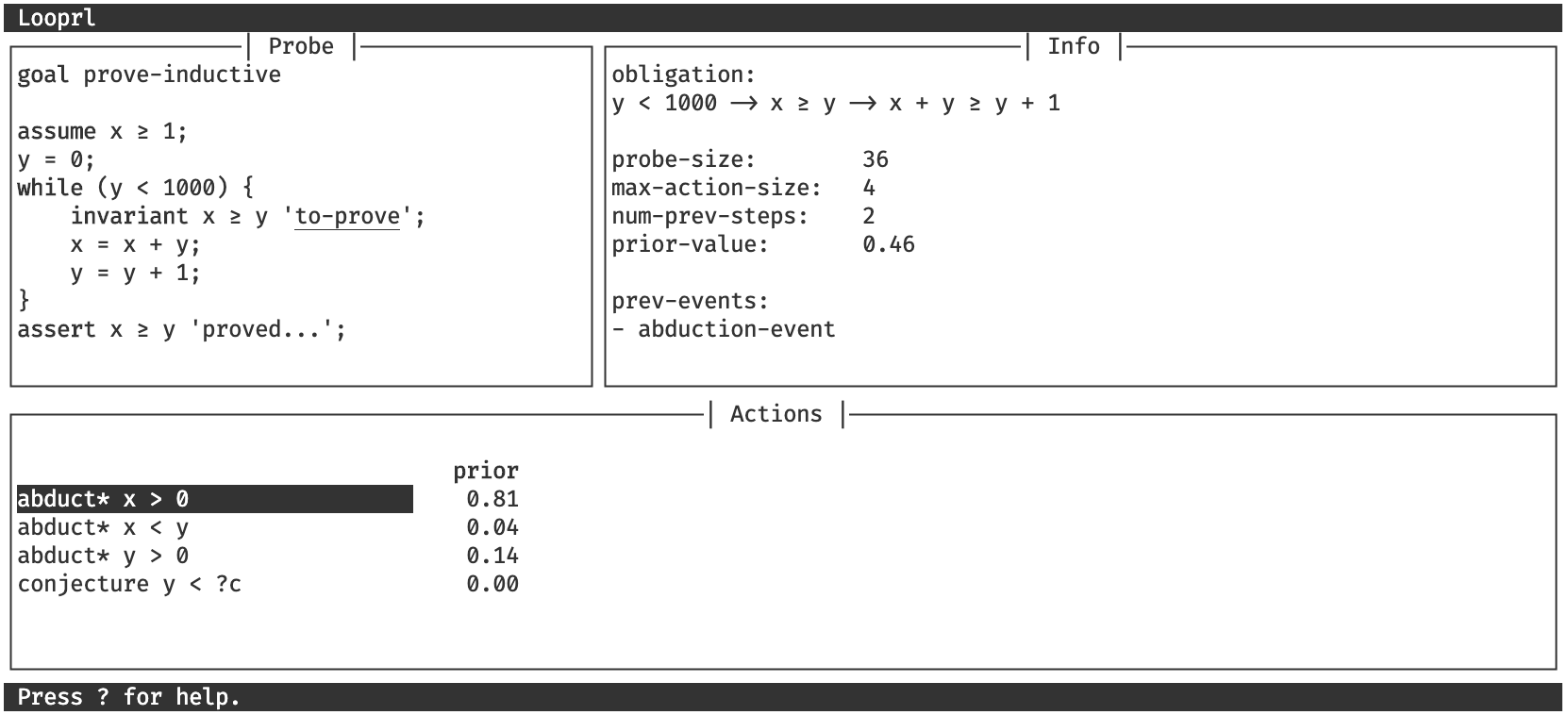
(a) Showing the proof obligation associated with the abduction call along with the neural network policy prior.

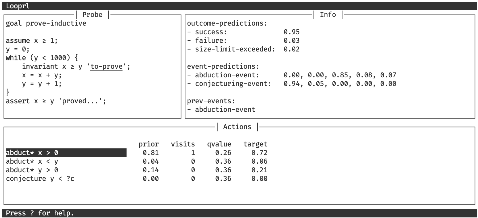
(b) Showing event predictions along with MCTS statistics.

Figure 8: Visualizing the solver strategy with the Looprl UI. In the screenshots above, the UI is used to examine a choice point in the solver strategy where the current invariant candidate $x\geq y$ cannot be proved to be inductive and the user must choose between proving one of several abduction candidates or making a conjecture (this roughly corresponds to the call to choose on line 33). Here, one can see the network assigning a high prior probability to the optimal proof action, which is to try and prove $x>0$ as an invariant. The network also predicts a value of $0.46$ for this state, which is close to the truth of $0.4$ (proving this problem requires three abduction events with cost $0.2$ each). The details of how the value is estimated can be consulted in screenshot 8(b). Here, we can see that the network predicts a $0.95$ probability of success along with a probability of $0.94$ for not requiring any conjecture and a probability of $0.85$ for needing two more abduction events.

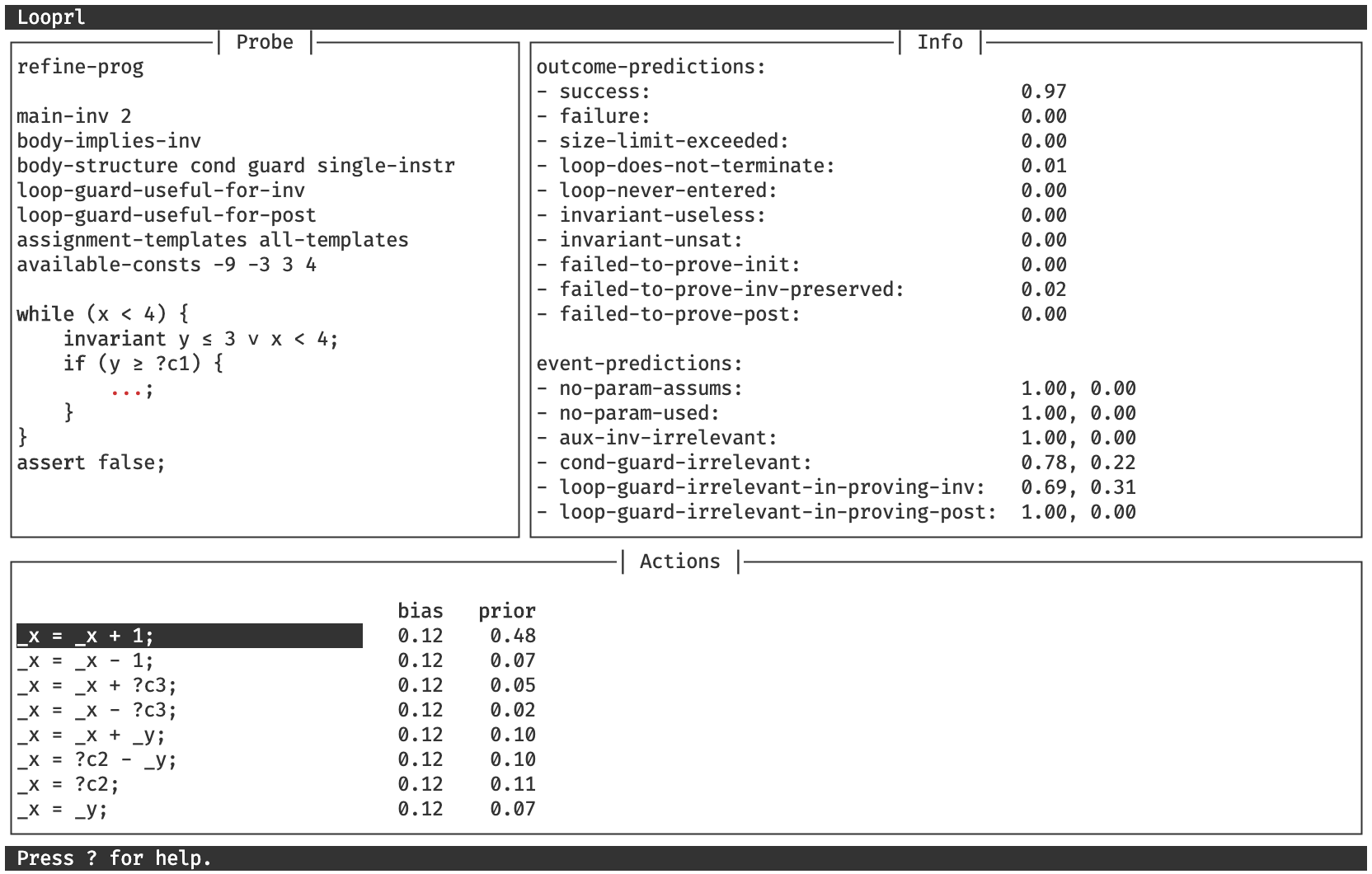
Figure 9: Visualizing the teacher strategy with the Looprl UI. This screenshot captures a choice point where the network is tasked with adding an assignment to the true branch of the conditional within the loop body. Several templates are proposed, which are going to be refined in turn. The upper left pane (i.e. the Probe pane) features all contextual information that is sent to the network to help it make a choice. Among this information, we can see a list of all constraints that the generated problem should ideally satisfy. The Info pane gives us some insights into the network’s prediction about future events and outcome. For example, the network estimates with $0.97$ probability that a valid problem will be generated (along with a $0.02$ probability that a failure will be encountered due to the invariant not being preserved by the loop body). The network also estimates a $31\%$ risk that the generated problem will violate the soft constraint according to which the loop guard should be relevant for proving the invariant.

Appendix F Implementing Abduction

Both the teacher and solver strategies we use as examples in this paper rely on an abduct function that takes as an input a formula $F$ and then either proves it valid or returns a (possibly empty) set of assumptions $A$ such that $A\ \rightarrow\ F$ can be proved to be valid.

Implementing such a function is hard in the general case and so an implementation of abduct may leverage nondeterminism. However, because we are only dealing with arithmetic of limited complexity in this work, we implemented a fully-specified abduction procedure for linear integer arithmetic that relies on Fourier-Motzkin elimination [45].

When given a formula $F$, our abduction procedure first rewrites it in conjunctive normal form as $F=\bigwedge_{i=1}^{n}\bigvee_{j}F_{ij}$ where $F_{ij}$ are atomic formulas of the form $\sum_{k}a_{k}x_{k}\odot c$ where $\odot\in\{\geq,=\}$ and $c,a_{k}$ are integer constants.

F.1 Case where $n=1$

If $F$ can be expressed as a disjunction of atomic formulas, we can compute abduction suggestions as follows: i) one considers the negation of $F$, obtaining a set of atomic assumptions and ii) one derives as many consequences as possible from those assumptions using Fourier-Motzkin elimination (linearly combining inequalities so as to eliminate variables). If a contradiction is derived, then $F$ is valid. If no contradiction is dervied given some timeout, then the negation of any derived consequence can be considered as an abduction candidate.

Example

Suppose we want to compute abduction candidates for $F=x\geq 0\ \rightarrow\ x+y\geq 1$. The conjunctive normal form of $F$ is $(x<0\,\vee\,x+y\geq 1)$. Taking the negation yields $(x\geq 0\,\wedge\,x+y<1)$, which we normalize into the set of assumptions $\{x\geq 0,-x-y\geq 0\}$ (all variables are integers). Then, we can take a Fourier-Motzkin step by adding these two assumptions and derive the following consequence: $-y\geq 0$. After this, no other reasoning step is applicable end we end up with the following set of facts: $\{x\geq 0,-x-y\geq 0,-y\geq 0\}$. We therefore suggest the following abduction candidates: $x<0$, $x+y>0$ and $y>0$.

F.2 Case where $n>1$

If the conjunctive normal form of $F$ has two conjuncts or more, we apply the procedure above on each conjunct separately. For example, suppose that $F=G\wedge H$, $G$ admits a set of abduction candidates $\{A_{i}\}_{i}$ and $H$ admits a set of abduction candidates $\{B_{i}\}_{i}$. One possibility would be to return all $\{A_{i}\wedge B_{j}\}_{ij}$ combinations as abduction candidates for $F$. However, doing so can quickly result in a combinatorial explosion. Therefore, our implementation does something different and returns the union of the $\{A_{i}\}_{i}$ and $\{B_{i}\}_{i}$ instead. Doing so, it cannot provide the guarantee that any resulting abduction candidate $A$ is sufficient in implying $F$. Rather, abduction candidates are seen as suggestions to unblock one part of the proof (i.e. enable proving one conjunct of $F$) but not necessarily the whole proof.

Appendix G Training Hyperparameters

We provide an exhaustive list of all hyperparameter values used in our experiments in Table LABEL:tab:hyperparams.

Table 8: Training hyperparameters for the experiments described in Section 4. Hyperparameters are organized according to a hierarchichal structure that is represented using indentation.

Parameter	Value	Description
params		[c]6cmAll hyperparameters.
*   teacher		[c]6cmHyperparameters for the teacher agent.
*    *   agent		[c]6cmHyperparameters common to all AlphaZero agents.
*    *    *   num-iters	[c]1.2cm20	[c]6cmTotal number of training iterations.
*    *    *   num-problems-per-iter	[c]1.2cm8000	[c]6cmNumber of data generation episodes per iteration.
*    *    *   num-validation-problems	[c]1.2cm800	[c]6cmNumber of validation-data generation episodes per iteration.
*    *    *   num-workers	[c]1.2cm600	[c]6cmNumber of episodes simulated in parallel or asynchronously during data generation.
*    *    *   num-processes	[c]1.2cmnone	[c]6cmNumber of distinct CPU processes spawned for data generation (by default, this value is set to the number of available physical CPU cores).
*    *    *   search		[c]6cmProof search limits.
*    *    *    *   max-proof-length	[c]1.2cm60	[c]6cmMaximum number of allowed environment steps before failing automatically.
*    *    *    *   max-probe-size	[c]1.2cm80	[c]6cmMaximum allowed size of state encodings. Bigger state encodings result in immediate failures.
*    *    *    *   max-action-size	[c]1.2cm12	[c]6cmMaximum allowed size of action encodings. Actions with bigger encodings are discarded.
*    *    *   encoding		[c]6cmState and action encoding hyperparameters.
*    *    *    *   d-model	[c]1.2cm128	[c]6cmEmbedding size for tokens, which is also equal to the neural network’s state dimension.
*    *    *    *   pos-enc-size	[c]1.2cm32	[c]6cmMaximal size of the tree positional encoding added to each token embedding.
*    *    *    *   uid-emb-size	[c]1.2cm16	[c]6cmMaximum number of unique identifiers that can be encoded.
*    *    *    *   const-emb-size	[c]1.2cm0	[c]6cmMaximum number of bits used to encode the binary value of numerical constants. No encoding is done if a value of 0 is provided.
*    *    *    *   enable-numerical-edges	[c]1.2cmtrue	[c]6cmAdd comparison edges between numerical constants.
*    *    *    *   add-reverse-edges	[c]1.2cmtrue	[c]6cmAdd reverse edges for all edge types.
*    *    *   network		[c]6cmHyperparameters for the Dynamic Graph Transformer network.
*    *    *    *   num-heads	[c]1.2cm4	[c]6cmNumber of transformer attention heads.
*    *    *    *   probe-encoder-layers	[c]1.2cm6	[c]6cmNumber of transformer blocks used to encode states.
*    *    *    *   action-encoder-layers	[c]1.2cm3	[c]6cmNumber of transformer blocks used to encode actions
*    *    *    *   combiner-layers	[c]1.2cm1	[c]6cmNumber of transformer blocks used in the combiner network that combines state and action encodings.
*    *    *    *   dropout-rate	[c]1.2cm0.05	[c]6cmDropout rate.
*    *    *    *   num-head-layers	[c]1.2cm2	[c]6cmNumber of layers in the feed-forward networks used for the value and policy heads.
*    *    *    *   head-dim	[c]1.2cm256	[c]6cmHidden dimension of layers in the feed-forward networks used for the value and policy heads.
*    *    *   mcts		[c]6cmMCTS hyperparameters.
*    *    *    *   num-simulations	[c]1.2cm64	[c]6cmNumber of MCTS simulations used for planning every environment step.
*    *    *    *   num-considered-actions	[c]1.2cm8	[c]6cmThe number of top-ranked actions that are considered in the sequential halving Gumbel exploration process.
*    *    *    *   value-scale	[c]1.2cm0.1	[c]6cmThe $c_{\text{scale}}$ hyperparameter (see original Gumbel AlphaZero paper).
*    *    *    *   max-visit-init	[c]1.2cm50	[c]6cmThe $c_{\text{visit}}$ hyperparameter (see original Gumbel AlphaZero paper).
*    *    *    *   fpu-red	[c]1.2cm0.1	[c]6cmValue estimates for unvisited children are decreased by this value so as to encourage deeper search trees (see LC0 AlphaZero implementation).
*    *    *    *   reset-tree	[c]1.2cmtrue	[c]6cmWhether the MCTS tree is reset after an environment move is taken.
*    *    *    *   max-tree-size	[c]1.2cm256	[c]6cmMaximal size of the MCTS tree. This parameter is relevant to avoid out-of-memory errors when reset-tree if false.
*    *    *    *   dirichlet-alpha	[c]1.2cm10	[c]6cmConcentration parameter for the Dirichlet exploration noise (see original AlphaZero paper).
*    *    *    *   dirichlet-eps	[c]1.2cm0.25	[c]6cmMagnitude of the Dirichlet exploration noise. No Dirichlet exploration noise is normally used with Gumbel AlphaZero but we add some anyway in the teacher for increased diversity.
*    *    *   training		[c]6cmNetwork training hyperparameters.
*    *    *    *   max-epochs	[c]1.2cm6	[c]6cmThe maximum number of training epochs.
*    *    *    *   improvement-required	[c]1.2cm1	[c]6cmGradient updates are stopped if the validation loss fails to decrease for more than this number of epochs.
*    *    *    *   batch-size	[c]1.2cm400	[c]6cmTraining batch size.
*    *    *    *   lr-base	[c]1.2cm0.0005	[c]6cmMaximal learning rate used in a cosine learning rate schedule with warm-up.
*    *    *    *   warmup-epochs	[c]1.2cm0.2	[c]6cmLength of the warm-up part of the learning rate schedule (in epochs).
*    *    *    *   weight-decay	[c]1.2cm0.01	[c]6cmWeight decay parameter.
*    *    *    *   outcome-loss-coeff	[c]1.2cm0.7	[c]6cmCoefficient for the loss term evaluating outcome prediction accuracy (e.g. success or failure).
*    *    *    *   event-loss-coeff	[c]1.2cm3	[c]6cmCoefficient for the loss term evaluating event prediction accuracy.
*    *    *    *   policy-loss-coeff	[c]1.2cm1	[c]6cmCoefficient for the loss term evaluating the divergence from policy priors to their targets.
*    *    *   training-window	[c]1.2cm1, 2, 2, 3, 3, 3, 4, 4, 4, 5, 5, 5, 6, 6, 6, 7	[c]6cmThe number of previous iterations from which samples are used to update the network at each iteration. If the provided list is shorter than the total number of iterations, the last number in this list is duplicated as many times as necessary.
*   solver		[c]6cmHyperparameters for the solver agent.
*    *   agent		[c]6cmHyperparameters common to all AlphaZero agents.
*    *    *   num-iters	[c]1.2cm20	[c]6cmTotal number of training iterations.
*    *    *   num-problems-per-iter	[c]1.2cm20000	[c]6cmNumber of data generation episodes per iteration.
*    *    *   num-validation-problems	[c]1.2cm5000	[c]6cmNumber of validation-data generation episodes per iteration.
*    *    *   num-workers	[c]1.2cm600	[c]6cmNumber of episodes simulated in parallel or asynchronously during data generation.
*    *    *   num-processes	[c]1.2cmnone	[c]6cmNumber of distinct CPU processes spawned for data generation (by default, this value is set to the number of available physical CPU cores).
*    *    *   search		[c]6cmProof search limits.
*    *    *    *   max-proof-length	[c]1.2cm12	[c]6cmMaximum number of allowed environment steps before failing automatically.
*    *    *    *   max-probe-size	[c]1.2cm80	[c]6cmMaximum allowed size of state encodings. Bigger state encodings result in immediate failures.
*    *    *    *   max-action-size	[c]1.2cm12	[c]6cmMaximum allowed size of action encodings. Actions with bigger encodings are discarded.
*    *    *   encoding		[c]6cmState and action encoding hyperparameters.
*    *    *    *   d-model	[c]1.2cm128	[c]6cmEmbedding size for tokens, which is also equal to the neural network’s state dimension.
*    *    *    *   pos-enc-size	[c]1.2cm32	[c]6cmMaximal size of the tree positional encoding added to each token embedding.
*    *    *    *   uid-emb-size	[c]1.2cm16	[c]6cmMaximum number of unique identifiers that can be encoded.
*    *    *    *   const-emb-size	[c]1.2cm0	[c]6cmMaximum number of bits used to encode the binary value of numerical constants. No encoding is done if a value of 0 is provided.
*    *    *    *   enable-numerical-edges	[c]1.2cmtrue	[c]6cmAdd comparison edges between numerical constants.
*    *    *    *   add-reverse-edges	[c]1.2cmtrue	[c]6cmAdd reverse edges for all edge types.
*    *    *   network		[c]6cmHyperparameters for the Dynamic Graph Transformer network.
*    *    *    *   num-heads	[c]1.2cm4	[c]6cmNumber of transformer attention heads.
*    *    *    *   probe-encoder-layers	[c]1.2cm6	[c]6cmNumber of transformer blocks used to encode states.
*    *    *    *   action-encoder-layers	[c]1.2cm3	[c]6cmNumber of transformer blocks used to encode actions
*    *    *    *   combiner-layers	[c]1.2cm1	[c]6cmNumber of transformer blocks used in the combiner network that combines state and action encodings.
*    *    *    *   dropout-rate	[c]1.2cm0.1	[c]6cmDropout rate.
*    *    *    *   num-head-layers	[c]1.2cm2	[c]6cmNumber of layers in the feed-forward networks used for the value and policy heads.
*    *    *    *   head-dim	[c]1.2cm256	[c]6cmHidden dimension of layers in the feed-forward networks used for the value and policy heads.
*    *    *   mcts		[c]6cmMCTS hyperparameters.
*    *    *    *   num-simulations	[c]1.2cm32	[c]6cmNumber of MCTS simulations used for planning every environment step.
*    *    *    *   num-considered-actions	[c]1.2cm8	[c]6cmThe number of top-ranked actions that are considered in the sequential halving Gumbel exploration process.
*    *    *    *   value-scale	[c]1.2cm0.1	[c]6cmThe $c_{\text{scale}}$ hyperparameter (see original Gumbel AlphaZero paper).
*    *    *    *   max-visit-init	[c]1.2cm50	[c]6cmThe $c_{\text{visit}}$ hyperparameter (see original Gumbel AlphaZero paper).
*    *    *    *   fpu-red	[c]1.2cm0	[c]6cmValue estimates for unvisited children are decreased by this value so as to encourage deeper search trees (see LC0 AlphaZero implementation).
*    *    *    *   reset-tree	[c]1.2cmfalse	[c]6cmWhether the MCTS tree is reset after an environment move is taken.
*    *    *    *   max-tree-size	[c]1.2cm256	[c]6cmMaximal size of the MCTS tree. This parameter is relevant to avoid out-of-memory errors when reset-tree if false.
*    *    *    *   dirichlet-alpha	[c]1.2cm10	[c]6cmConcentration parameter for the Dirichlet exploration noise (see original AlphaZero paper).
*    *    *    *   dirichlet-eps	[c]1.2cmnone	[c]6cmMagnitude of the Dirichlet exploration noise. No Dirichlet exploration noise is normally used with Gumbel AlphaZero but we add some anyway in the teacher for increased diversity.
*    *    *   training		[c]6cmNetwork training hyperparameters.
*    *    *    *   max-epochs	[c]1.2cm1	[c]6cmThe maximum number of training epochs.
*    *    *    *   improvement-required	[c]1.2cm1	[c]6cmGradient updates are stopped if the validation loss fails to decrease for more than this number of epochs.
*    *    *    *   batch-size	[c]1.2cm300	[c]6cmTraining batch size.
*    *    *    *   lr-base	[c]1.2cm0.0003	[c]6cmMaximal learning rate used in a cosine learning rate schedule with warm-up.
*    *    *    *   warmup-epochs	[c]1.2cm0.2	[c]6cmLength of the warm-up part of the learning rate schedule (in epochs).
*    *    *    *   weight-decay	[c]1.2cm0.01	[c]6cmWeight decay parameter.
*    *    *    *   outcome-loss-coeff	[c]1.2cm1	[c]6cmCoefficient for the loss term evaluating outcome prediction accuracy (e.g. success or failure).
*    *    *    *   event-loss-coeff	[c]1.2cm1	[c]6cmCoefficient for the loss term evaluating event prediction accuracy.
*    *    *    *   policy-loss-coeff	[c]1.2cm1	[c]6cmCoefficient for the loss term evaluating the divergence from policy priors to their targets.
*    *    *   training-window	[c]1.2cm1, 2, 2, 3, 3, 3, 4, 4, 4, 5, 5, 5, 6, 6, 6, 7	[c]6cmThe number of previous iterations from which samples are used to update the network at each iteration. If the provided list is shorter than the total number of iterations, the last number in this list is duplicated as many times as necessary.
*   num-teacher-iters-used-by-solver	[c]1.2cm5	[c]6cmThe number of teacher training iterations from which solver training samples are collected.
*   extra-teacher-problems	[c]1.2cm10000	[c]6cmNumber of extra teacher problems that are generated once the teacher is trained, with no exploration noise.

Appendix H Network Architecture and Choice Points Encoding

H.1 Network Architecture

Neural networks that are used as oracles for nondeterministic strategies take as an input a choice point and return i) a probability distribution over all available choices, ii) some success and failure probability estimates and iii) some event occurence probability estimates (see Section 2.5). In turn, a choice point is represented as i) a probe [10] that encodes all relevant state information provided to choose (see Figure 7 for examples) and ii) a list of possible choices that were passed as arguments to choose.

Our proposed network architecture works as follows. Given a choice point, the probe is encoded using a Dynamic Graph Transformer (DGT) neural network [32]. DGT networks are similar to Transformers [46] but they allow leveraging some additional graph structure over the source tokens by associating edge types to learned attention biases. Each choice is encoded separately using another DGT. It is then concatenated with the probe encoding and passed to a combiner network that outputs a score. Scores are normalized into a probability distribution using a softmax operation. The probe encoding is also passed to a value head that produces outcome and event predictions. Batches of choice points can be evaluated efficiently in parallel using scatter operations [47].

H.2 Encoding Programs and Formulas

All data that is to be passed to the neural network must be encodable into a sequence of tokens with an optional graph structure. This is the case of programs and formulas in particular. We use standard techniques to encode those [48, 49]:

• Abstract syntax trees (ASTs) are encoded into a sequence of tokens in polish notation order (e.g. $x+3y$ is encoded as “PLUS VAR(x) MUL CONST(3) VAR(y)”). The edges in the original AST are preserved as graph edges to be passed to the DGT network.

• We use a different positional encoding scheme for tokens that leverages the tree structure of the underlying AST [49]. Doing so has been demonstrated to result in better generalization capabilities [50].

• Identifier names are randomly mapped into a finite number of unique ids for each choice point. Unique ids are encoded using a one-hot encoding scheme. If a choice point introduces more names than there are unique ids available (rare), the last occuring names are made to share a single uid that is flagged to indicate a naming conflict.

• Numerical constants with an absolute value greater than $3$ are represented with generic POS_CONST and NEG_CONST tokens. A binary encoding of their value is also provided to the network. Moreover, special edges are added to compare all numerical constants involved in a program or formula (see Table LABEL:tab:edges).

• Following [48], we also add semantic edges to the encoding of programs and formulas that reflect the way information flows within them. Details can be consulted in Table LABEL:tab:edges.

Edge type	Description
PARENT	Connect any token to its parent in the syntax tree.
PREV_SIBLING	Connect any token to its previous sibling in the syntax tree.
PREV_LEXICAL_USE	Connect any token associated with name $s$ to the previous occurence of $s$.
LAST_READ	Connect a variable occurence to places where it was possibly read last.
LAST_WRITE	Connect a variable occ. to places where it was possibly written last.
GUARDED_BY	Connect a variable occ. to assumptions made about it.
GUARDED_BY_NEG	Connect a variable occ. to negated assumptions made about it.
COMPUTED_FROM	Connect the lhs of any assignment to the variables in its rhs.
SAME_CONST	Connect two identical numerical constants.
SMALLER_CONST	Compare two different numerical constants.

References

- [1] Daniel Huang, Prafulla Dhariwal, Dawn Song, and Ilya Sutskever. GamePad: A learning environment for theorem proving. In 7th International Conference on Learning Representations, ICLR 2019, New Orleans, LA, USA, May 6-9, 2019. OpenReview.net, 2019.
- [2] Kaiyu Yang and Jia Deng. Learning to prove theorems via interacting with proof assistants. In Kamalika Chaudhuri and Ruslan Salakhutdinov, editors, Proceedings of the 36th International Conference on Machine Learning, ICML 2019, 9-15 June 2019, Long Beach, California, USA, volume 97 of Proceedings of Machine Learning Research, pages 6984–6994. PMLR, 2019.
- [3] Kshitij Bansal, Sarah M. Loos, Markus N. Rabe, Christian Szegedy, and Stewart Wilcox. HOList: an environment for machine learning of higher order logic theorem proving. In Kamalika Chaudhuri and Ruslan Salakhutdinov, editors, Proceedings of the 36th International Conference on Machine Learning, ICML 2019, 9-15 June 2019, Long Beach, California, USA, volume 97 of Proceedings of Machine Learning Research, pages 454–463. PMLR, 2019.
- [4] Wenda Li, Lei Yu, Yuhuai Wu, and Lawrence C. Paulson. IsarStep: a benchmark for high-level mathematical reasoning. In 9th International Conference on Learning Representations, ICLR 2021, Virtual Event, Austria, May 3-7, 2021. OpenReview.net, 2021.
- [5] Jesse Michael Han, Jason Rute, Yuhuai Wu, Edward W. Ayers, and Stanislas Polu. Proof artifact co-training for theorem proving with language models. In The Tenth International Conference on Learning Representations, ICLR 2022, Virtual Event, April 25-29, 2022. OpenReview.net, 2022.
- [6] Mingzhe Wang and Jia Deng. Learning to prove theorems by learning to generate theorems. In Hugo Larochelle, Marc’Aurelio Ranzato, Raia Hadsell, Maria-Florina Balcan, and Hsuan-Tien Lin, editors, Advances in Neural Information Processing Systems 33: Annual Conference on Neural Information Processing Systems 2020, NeurIPS 2020, December 6-12, 2020, virtual, 2020.
- [7] David Silver, Thomas Hubert, Julian Schrittwieser, Ioannis Antonoglou, Matthew Lai, Arthur Guez, Marc Lanctot, Laurent Sifre, Dharshan Kumaran, Thore Graepel, et al. A general reinforcement learning algorithm that masters chess, shogi, and go through self-play. Science, 362(6419):1140–1144, 2018.
- [8] Kshitij Bansal, Sarah M. Loos, Markus N. Rabe, and Christian Szegedy. Learning to reason in large theories without imitation. CoRR, abs/1905.10501, 2019.
- [9] Minchao Wu, Michael Norrish, Christian Walder, and Amir Dezfouli. TacticZero: learning to prove theorems from scratch with deep reinforcement learning. In Marc’Aurelio Ranzato, Alina Beygelzimer, Yann N. Dauphin, Percy Liang, and Jennifer Wortman Vaughan, editors, Advances in Neural Information Processing Systems 34: Annual Conference on Neural Information Processing Systems 2021, NeurIPS 2021, December 6-14, 2021, virtual, pages 9330–9342, 2021.
- [10] Daniel Selsam. Beyond the tactic-state automaton. Mathematical Reasoning in General Artificial Intelligence Workshop, ICLR, 2021.
- [11] Reiner Hähnle and Peter H. Schmitt. The liberalized -rule in free variable semantic tableaux. J. Autom. Reasoning, 13(2):211–221, 1994.
- [12] Stephen A. Cook. Soundness and completeness of an axiom system for program verification. SIAM J. Comput., 7(1):70–90, 1978.
- [13] David Harel. First-Order Dynamic Logic, volume 68 of LNCS. Springer, 1979.
- [14] Jean-Christophe Filliâtre. One logic to use them all. In Maria Paola Bonacina, editor, Automated Deduction - CADE-24 - 24th International Conference on Automated Deduction, Lake Placid, NY, USA, June 9-14, 2013. Proceedings, volume 7898 of LNCS, pages 1–20. Springer, 2013.
- [15] C. A. R. Hoare. An axiomatic basis for computer programming. Commun. ACM, 12(10):576–580, 1969.
- [16] Michael Meyer. Abduction – a logical view for investigating and initiating processes of discovering mathematical coherences. Educational Studies in Mathematics, 74(2):185–205, 2010.
- [17] George Polya. How to solve it: A new aspect of mathematical method, volume 85. Princeton university press, 2004.
- [18] Isil Dillig, Thomas Dillig, Boyang Li, and Kenneth L. McMillan. Inductive invariant generation via abductive inference. In Antony L. Hosking, Patrick Th. Eugster, and Cristina V. Lopes, editors, Proceedings of the 2013 ACM SIGPLAN International Conference on Object Oriented Programming Systems Languages & Applications, OOPSLA 2013, part of SPLASH 2013, Indianapolis, IN, USA, October 26-31, 2013, pages 443–456. ACM, 2013.
- [19] Mnacho Echenim, Nicolas Peltier, and Yanis Sellami. Ilinva: using abduction to generate loop invariants. In Andreas Herzig and Andrei Popescu, editors, Frontiers of Combining Systems - 12th International Symposium, FroCoS 2019, London, UK, September 4-6, 2019, Proceedings, volume 11715 of LNCS, pages 77–93. Springer, 2019.
- [20] Thomas Eiter and Georg Gottlob. The complexity of logic-based abduction. J. ACM, 42(1):3–42, 1995.
- [21] Ivo Danihelka, Arthur Guez, Julian Schrittwieser, and David Silver. Policy improvement by planning with Gumbel. In The Tenth International Conference on Learning Representations, ICLR 2022, Virtual Event, April 25-29, 2022. OpenReview.net, 2022.
- [22] Cameron Browne, Edward Jack Powley, Daniel Whitehouse, Simon M. Lucas, Peter I. Cowling, Philipp Rohlfshagen, Stephen Tavener, Diego Perez Liebana, Spyridon Samothrakis, and Simon Colton. A survey of Monte Carlo Tree Search methods. IEEE Trans. Comput. Intell. AI Games, 4(1):1–43, 2012.
- [23] Rudy Bunel, Matthew J. Hausknecht, Jacob Devlin, Rishabh Singh, and Pushmeet Kohli. Leveraging grammar and reinforcement learning for neural program synthesis. In 6th International Conference on Learning Representations, ICLR 2018, Vancouver, BC, Canada, April 30 - May 3, 2018, Conference Track Proceedings. OpenReview.net, 2018.
- [24] Guillaume Lample and François Charton. Deep learning for symbolic mathematics. In 8th International Conference on Learning Representations, ICLR 2020, Addis Ababa, Ethiopia, April 26-30, 2020. OpenReview.net, 2020.
- [25] David J. Wu. Accelerating self-play learning in go. CoRR, abs/1902.10565, 2019.
- [26] Adam Paszke, Sam Gross, Francisco Massa, Adam Lerer, James Bradbury, Gregory Chanan, Trevor Killeen, Zeming Lin, Natalia Gimelshein, Luca Antiga, Alban Desmaison, Andreas Köpf, Edward Z. Yang, Zachary DeVito, Martin Raison, Alykhan Tejani, Sasank Chilamkurthy, Benoit Steiner, Lu Fang, Junjie Bai, and Soumith Chintala. Pytorch: An imperative style, high-performance deep learning library. In Hanna M. Wallach, Hugo Larochelle, Alina Beygelzimer, Florence d’Alché-Buc, Emily B. Fox, and Roman Garnett, editors, Advances in Neural Information Processing Systems 32: Annual Conference on Neural Information Processing Systems 2019, NeurIPS 2019, December 8-14, 2019, Vancouver, BC, Canada, pages 8024–8035, 2019.
- [27] Philipp Moritz, Robert Nishihara, Stephanie Wang, Alexey Tumanov, Richard Liaw, Eric Liang, Melih Elibol, Zongheng Yang, William Paul, Michael I. Jordan, and Ion Stoica. Ray: A distributed framework for emerging AI applications. In Andrea C. Arpaci-Dusseau and Geoff Voelker, editors, 13th USENIX Symposium on Operating Systems Design and Implementation, OSDI 2018, Carlsbad, CA, USA, October 8-10, 2018, pages 561–577. USENIX Association, 2018.
- [28] Jules Hedges. Monad transformers for backtracking search. In Paul Blain Levy and Neel Krishnaswami, editors, Proceedings 5th Workshop on Mathematically Structured Functional Programming, MSFP@ETAPS 2014, Grenoble, France, 12 April 2014, volume 153 of EPTCS, pages 31–50, 2014.
- [29] Xujie Si, Hanjun Dai, Mukund Raghothaman, Mayur Naik, and Le Song. Learning loop invariants for program verification. In Advances in Neural Information Processing Systems, pages 7762–7773, 2018.
- [30] Xujie Si, Aaditya Naik, Hanjun Dai, Mayur Naik, and Le Song. Code2inv: A deep learning framework for program verification. In Shuvendu K. Lahiri and Chao Wang, editors, Computer Aided Verification - 32nd International Conference, CAV 2020, Los Angeles, CA, USA, July 21-24, 2020, Proceedings, Part II, volume 12225 of LNCS, pages 151–164. Springer, 2020.
- [31] Gabriel Ryan, Justin Wong, Jianan Yao, Ronghui Gu, and Suman Jana. CLN2INV: learning loop invariants with continuous logic networks. In 8th International Conference on Learning Representations, ICLR 2020, Addis Ababa, Ethiopia, April 26-30, 2020. OpenReview.net, 2020.
- [32] Daniel Selsam, Jesse Michael Han, Leonardo de Moura, and Patrice Godefroid. Universal policies for software-defined MDPs. arXiv preprint arXiv:2012.11401, 2020.
- [33] Daniel Selsam. The IMO grand challenge. http://aitp-conference.org/2020/slides/DS.pdf, 2020. Talk at AITP 2020.
- [34] Daniel Selsam. The IMO grand challenge: A battle of ideas. https://dselsam.github.io/IMO-GC-battle-of-ideas/, 2020.
- [35] Yuhuai Wu, Albert Q. Jiang, Jimmy Ba, and Roger Baker Grosse. INT: an inequality benchmark for evaluating generalization in theorem proving. In 9th International Conference on Learning Representations, ICLR 2021, Virtual Event, Austria, May 3-7, 2021. OpenReview.net, 2021.
- [36] Eser Aygün, Zafarali Ahmed, Ankit Anand, Vlad Firoiu, Xavier Glorot, Laurent Orseau, Doina Precup, and Shibl Mourad. Learning to prove from synthetic theorems. CoRR, abs/2006.11259, 2020.
- [37] Yury Puzis, Yi Gao, and Geoff Sutcliffe. Automated generation of interesting theorems. In Geoff Sutcliffe and Randy Goebel, editors, Proceedings of the Nineteenth International Florida Artificial Intelligence Research Society Conference, Melbourne Beach, Florida, USA, May 11-13, 2006, pages 49–54. AAAI Press, 2006.
- [38] Stanislas Polu and Ilya Sutskever. Generative language modeling for automated theorem proving. CoRR, abs/2009.03393, 2020.
- [39] Cezary Kaliszyk, Josef Urban, Henryk Michalewski, and Miroslav Olsák. Reinforcement learning of theorem proving. In Samy Bengio, Hanna M. Wallach, Hugo Larochelle, Kristen Grauman, Nicolò Cesa-Bianchi, and Roman Garnett, editors, Advances in Neural Information Processing Systems 31: Annual Conference on Neural Information Processing Systems 2018, NeurIPS 2018, December 3-8, 2018, Montréal, Canada, pages 8836–8847, 2018.
- [40] Maxwell Crouse, Ibrahim Abdelaziz, Bassem Makni, Spencer Whitehead, Cristina Cornelio, Pavan Kapanipathi, Kavitha Srinivas, Veronika Thost, Michael Witbrock, and Achille Fokoue. A deep reinforcement learning approach to first-order logic theorem proving. In Thirty-Fifth AAAI Conference on Artificial Intelligence, AAAI 2021, Thirty-Third Conference on Innovative Applications of Artificial Intelligence, IAAI 2021, The Eleventh Symposium on Educational Advances in Artificial Intelligence, EAAI 2021, Virtual Event, February 2-9, 2021, pages 6279–6287. AAAI Press, 2021.
- [41] Timothy Gowers. How can it be feasible to find proofs? https://gowers.wordpress.com/2022/04/28/announcing-an-automatic-theorem-proving-project/, 2022.
- [42] David Delahaye. A tactic language for the system Coq. In Michel Parigot and Andrei Voronkov, editors, Logic for Programming and Automated Reasoning, 7th International Conference, LPAR 2000, Reunion Island, France, November 11-12, 2000, Proceedings, volume 1955 of LNCS, pages 85–95. Springer, 2000.
- [43] Adam Chlipala. Certified Programming with Dependent Types - A Pragmatic Introduction to the Coq Proof Assistant. MIT Press, 2013.
- [44] Nathan Fulton, Stefan Mitsch, Brandon Bohrer, and André Platzer. Bellerophon: Tactical theorem proving for hybrid systems. In Mauricio Ayala-Rincón and César A. Muñoz, editors, ITP, volume 10499 of LNCS, pages 207–224. Springer, 2017.
- [45] George B. Dantzig and B. Curtis Eaves. Fourier-Motzkin elimination and its dual. J. Comb. Theory, Ser. A, 14(3):288–297, 1973.
- [46] Ashish Vaswani, Noam Shazeer, Niki Parmar, Jakob Uszkoreit, Llion Jones, Aidan N. Gomez, Lukasz Kaiser, and Illia Polosukhin. Attention is all you need. In Isabelle Guyon, Ulrike von Luxburg, Samy Bengio, Hanna M. Wallach, Rob Fergus, S. V. N. Vishwanathan, and Roman Garnett, editors, Advances in Neural Information Processing Systems 30: Annual Conference on Neural Information Processing Systems 2017, December 4-9, 2017, Long Beach, CA, USA, pages 5998–6008, 2017.
- [47] Matthias Fey and Jan E. Lenssen. Fast graph representation learning with PyTorch Geometric. In ICLR Workshop on Representation Learning on Graphs and Manifolds, 2019.
- [48] Vincent J. Hellendoorn, Charles Sutton, Rishabh Singh, Petros Maniatis, and David Bieber. Global relational models of source code. In 8th International Conference on Learning Representations, ICLR 2020, Addis Ababa, Ethiopia, April 26-30, 2020. OpenReview.net, 2020.
- [49] Vighnesh Leonardo Shiv and Chris Quirk. Novel positional encodings to enable tree-based transformers. In Hanna M. Wallach, Hugo Larochelle, Alina Beygelzimer, Florence d’Alché-Buc, Emily B. Fox, and Roman Garnett, editors, Advances in Neural Information Processing Systems 32: Annual Conference on Neural Information Processing Systems 2019, NeurIPS 2019, December 8-14, 2019, Vancouver, BC, Canada, pages 12058–12068, 2019.
- [50] Christopher Hahn, Frederik Schmitt, Jens U. Kreber, Markus Norman Rabe, and Bernd Finkbeiner. Teaching temporal logics to neural networks. In 9th International Conference on Learning Representations, ICLR 2021, Virtual Event, Austria, May 3-7, 2021. OpenReview.net, 2021.