MIP-GNN: A Data-Driven Framework for Guiding Combinatorial Solvers

Abstract

Mixed-integer programming (MIP) technology offers a generic way of formulating and solving combinatorial optimization problems. While generally reliable, state-of-the-art MIP solvers base many crucial decisions on hand-crafted heuristics, largely ignoring common patterns within a given instance distribution of the problem of interest. Here, we propose MIP-GNN, a general framework for enhancing such solvers with data-driven insights. By encoding the variable-constraint interactions of a given mixed-integer linear program (MILP) as a bipartite graph, we leverage state-of-the-art graph neural network architectures to predict variable biases, i.e., component-wise averages of (near) optimal solutions, indicating how likely a variable will be set to 0 or 1 in (near) optimal solutions of binary MILPs. In turn, the predicted biases stemming from a single, once-trained model are used to guide the solver, replacing heuristic components. We integrate MIP-GNN into a state-of-the-art MIP solver, applying it to tasks such as node selection and warm-starting, showing significant improvements compared to the default setting of the solver on two classes of challenging binary MILPs. Our code and appendix are publicly available at https://github.com/lyeskhalil/mipGNN.

Introduction

Nowadays, combinatorial optimization (CO) is an interdisciplinary field spanning optimization, operations research, discrete mathematics, and computer science, with many critical real-world applications such as vehicle routing or scheduling; see, e.g., (Korte and Vygen 2012) for a general overview. Mixed-integer programming technology offers a generic way of formulating and solving CO problems by relying on combinatorial solvers based on tree search algorithms, such as branch and cut, see, e.g., (Nemhauser and Wolsey 1988; Schrijver 1999; Bertsimas and Weismantel 2005). Given enough time, these algorithms find certifiably optimal solutions to NP-hard problems. However, many essential decisions in the search process, e.g., node and variable selection, are based on heuristics (Lodi 2013). The design of these heuristics relies on intuition and empirical evidence, largely ignoring that, in practice, one often repeatedly solves problem instances that share patterns and characteristics. Machine learning approaches have emerged to address this shortcoming, enhancing state-of-the-art solvers with data-driven insights (Bengio, Lodi, and Prouvost 2021; Cappart et al. 2021; Kotary et al. 2021).

Many CO problems can be naturally described using graphs, either as direct input (e.g., routing on road networks) or by encoding variable-constraint interactions (e.g., of a MILP model) as a bipartite graph. As such, machine learning approaches such as graph neural networks (GNNs) (Gilmer et al. 2017; Scarselli et al. 2009) have recently helped bridge the gap between machine learning, relational inputs, and combinatorial optimization (Cappart et al. 2021). GNNs compute vectorial representations of each node in the input graph in a permutation-equivariant fashion by iteratively aggregating features of neighboring nodes. By parameterizing this aggregation step, a GNN is trained end-to-end against a loss function to adapt to the given data distribution. Hence, GNNs can be viewed as a relational inductive bias (Battaglia et al. 2018), encoding crucial graph structures underlying the CO/MIP instance distribution of interest.

Present Work

We introduce MIP-GNN, a general GNN-based framework for guiding state-of-the-art branch-and-cut solvers on (binary) mixed-integer linear programs. Specifically, we encode the variable-constraint interactions of a MILP as a bipartite graph where a pair of variable/constraint nodes share an edge iff the variable has a non-zero coefficient in the constraint; see Figure 1. To guide a solver in finding a solution or certifying optimality faster for a given instance, we perform supervised GNN training to predict variable biases (Hsu et al. 2008), which are computed by component-wise averaging over a set of near-optimal solutions of a given MILP. Intuitively, these biases encode how likely it is for a variable to take a value of 1 in near-optimal solutions. To tailor the GNN more closely to the task of variable bias prediction, we propagate a “residual error”, indicating how much the current assignment violates the constraints. Further, the theory, outlined in the appendix, gives some initial insights into the theoretical capabilities of such GNNs architecture in the context of MILPs.

We integrate such trained GNNs into a state-of-the-art MIP solver, namely CPLEX (IBM 2020), by using the GNN’s variable bias prediction in crucial tasks within the branch-and-cut algorithm, such as node selection and warm-starting. On a large set of diverse, real-world binary MILPs, modeling the generalized independent set problem (Colombi, Mansini, and Savelsbergh 2017) and a fixed-charge multi-commodity network flow problem (Hewitt, Nemhauser, and Savelsbergh 2010), we show significant improvements over default CPLEX for the task of node selection, while also reporting promising performance for warm-starting and branching variable selection. This is achieved without any feature engineering, i.e., by relying purely on the graph information induced by the given MILP.

Crucially, for the first time in this line of research, we use a single, once-trained model for bias prediction to speed up multiple components of the MIP branch and cut simultaneously. In other words, we show that learning the bias associated with sets of near-optimal solutions is empirically beneficial to multiple crucial MIP ingredients.

Figure 1: MIP-GNN predicts variables biases for node selection.

Related Work

GNNs Graph neural networks (GNNs) (Gilmer et al. 2017; Scarselli et al. 2009) have emerged as a flexible framework for machine learning on graphs and relational data. Notable instances of this architecture include, e.g., (Duvenaud et al. 2015; Hamilton, Ying, and Leskovec 2017; Veličković et al. 2018), and the spectral approaches proposed in, e.g., (Bruna et al. 2014; Defferrard, Bresson, and Vandergheynst 2016; Kipf and Welling 2017)—all of which descend from early work in (Baskin, Palyulin, and Zefirov 1997; Kireev 1995; Merkwirth and Lengauer 2005; Micheli 2009; Micheli and Sestito 2005; Scarselli et al. 2009; Sperduti and Starita 1997). Surveys of recent advancements in GNN techniques can be found in (Chami et al. 2020; Wu et al. 2019).

Machine learning for CO Bengio, Lodi, and Prouvost (2021) discuss and review machine learning approaches to enhance combinatorial optimization. Concrete examples include the imitation of computationally demanding variable selection rules within the branch-and-cut framework (Khalil et al. 2016; Zarpellon et al. 2020), learning to run (primal) heuristics (Khalil et al. 2017; Chmiela et al. 2021), learning decompositions of large MILPs for scalable heuristic solving (Song et al. 2020), or leveraging machine learning to find (primal) solutions to stochastic integer problems quickly (Bengio et al. 2020). See (Kotary et al. 2021) for a high-level overview of recent advances.

GNNs for CO Many prominent CO problems involve graph or relational structures, either directly given as input or induced by the variable-constraint interactions. Recent progress in using GNNs to bridge the gap between machine learning and combinatorial optimization are surveyed in (Cappart et al. 2021). Works in the field can be categorized between approaches directly using GNNs to output solutions without relying on solvers and approaches replacing the solver’s heuristic components with data-driven ones.

Representative works of the first kind include (Dai et al. 2017), where GNNs served as the function approximator for the value function in a Deep $Q$-learning (DQN) formulation of CO on graphs. The authors used a GNN to embed nodes of the input graph. Through the combination of GNN and DQN, a greedy node selection policy is learned on a set of problem instances drawn from the same distribution. Kool, Van Hoof, and Welling (2019) addressed routing-type problems by training an encoder-decoder architecture, based on Graph Attention Networks (Veličković et al. 2018), by using an Actor-Critic reinforcement approach. Joshi, Laurent, and Bresson (2019) proposed the use of residual gated graph convolutional networks (Bresson and Laurent 2017) in a supervised manner to predict solutions to the traveling salesperson problem. Fey et al. (2020) and Li et al. (2019) use GNNs for supervised learning of matching or alignment problems, whereas Kurin et al. (2020); Selsam and Bjørner (2019); Selsam et al. (2019) used them to find assignments satisfying logical formulas. Moreover, Toenshoff et al. (2019) and Karalias and Loukas (2020) explored unsupervised approaches, encoding constraints into the loss function.

Works that integrate GNNs in a combinatorial solver conserve its optimality guarantees. Gasse et al. (2019) proposed to encode the variable constraint interaction of a MILP as a bipartite graph and trained a GNN in a supervised fashion to imitate costly variable selection rules within the branch-and-cut framework of the SCIP solver (Gamrath et al. 2020). Building on that, Gupta et al. (2020) proposed a hybrid branching model using a GNN at the initial decision point and a light multilayer perceptron for subsequent steps, showing improvements on pure CPU machines. Finally, Nair et al. (2020) expanded the GNN approach to branching by implementing a GPU-friendly parallel linear programming solver using the alternating direction method of multipliers that allows scaling the strong branching expert to substantially larger instances, also combining this innovation with a novel GNN approach to diving.

Closest to the present work, Ding et al. (2020) used GNNs on a tripartite graph consisting of variables, constraints and a single objective node, enriched with hand-crafted node features. The target is to predict the 0-1 values of the so-called stable variables, i.e., variables whose assignment does not change over a set of pre-computed feasible solutions. The predictions then define a “local branching” constraint (Fischetti and Lodi 2003) which can be used in an exact or heuristic way; the latter restricts the search to solutions that differ in at most a handful of the variables predicted to be “stable”. MIP-GNN differs in the prediction target (biases vs. stable variables), the labeling strategy (leveraging the “solution pool” of modern MIP solvers vs. primal heuristics), not relying on any feature engineering, flexible GNN architecture choices and evaluation, more robust downstream uses of the predictions via node selection and warm-starting, and tackling much more challenging problem classes.

Preliminaries

Notation

Let $[n]=\{1,\dotsc,n\}\subset\mathbb{N}$ for $n\geq 1$, and let $\{\!\!\{\dots\}\!\!\}$ denote a multiset. A graph $G$ is a pair $(V,E)$ with a finite set of nodes $V$ and a set of edges $E\subseteq V\times V$. In most cases, we interpret $G$ as an undirected graph. We denote the set of nodes and the set of edges of $G$ by $V(G)$ and $E(G)$, respectively. We enrich the nodes and the edges of a graph with features, i.e., a mapping $l\colon V(G)\cup E(G)\to\mathbb{R}^{d}$. Moreover, $l(x)$ is a feature of $x$, for $x$ in $V(G)\cup E(G)$. The neighborhood of $v$ in $V(G)$ is denoted by $N(v)=\{u\in V(G)\mid(v,u)\in E(G)\}$. A bipartite graph is a tuple $(A,B,E)$, where $(A\sqcup B,E)$ is a graph, and every edge connects a node in $A$ with a node in $B$. Let $f\colon S\to\mathbb{R}^{d}$ for some arbitrary domain $S$. Then $\mathbf{f}(s)\in\mathbb{R}^{d}$, $s$ in $S$, denotes the real-valued vector resulting from applying $f$ entry-wise to $s$. Last, $[\cdot]$ denotes column-wise (vector) concatenation.

Linear and Mixed-Integer Programs

A linear program (LP) aims at optimizing a linear function over a feasible set described as the intersection of finitely many halfspaces, i.e., a polyhedron. We restrict our attention to feasible and bounded LPs. Formally, an instance $I$ of an LP is a tuple $(\mathbf{A},\mathbf{b},\mathbf{c})$, where $\mathbf{A}$ is a matrix in $\mathbb{Q}^{m\times n}$, and $\mathbf{b}$ and ${c}$ are vectors in $\mathbb{Q}^{m}$ and $\mathbb{Q}^{n}$, respectively. We aim at finding a vector $\mathbf{x}^{*}$ in $\mathbb{Q}^{n}$ that minimizes $\mathbf{c}^{T}\mathbf{x}^{*}$ over the feasible set

$$F(I)=\{\mathbf{x}\in\mathbb{Q}^{n}\mid \mathbf{A}_{j}\mathbf{x}\leq b_{j}\text{ for }j\in[m]\text{ and }$$

$$x_{i}\geq 0\text{ for }i\in[n]\}.$$

In practice, LPs are solved using the Simplex method or (weakly) polynomial-time interior point methods (Bertsimas and Tsitsiklis 1997). Due to their continuous nature, LPs are not suitable to encode the feasible set of a CO problem. Hence, we extend LPs by adding integrality constraints, i.e., requiring that the value assigned to each entry of $\mathbf{x}$ is an integer. Consequently, we aim to find the vector $\mathbf{x}^{*}$ in $\mathbb{Z}^{n}$ that minimizes $\mathbf{c}^{T}\mathbf{x}^{*}$ over the feasible set

$$F_{\textsf{Int}}(I)=\{\mathbf{x}\in\mathbb{Z}^{n}\mid \mathbf{A}_{j}\mathbf{x}\leq b_{j}\text{ for }j\in[m],x_{i}\geq 0,\text{ and }$$

$$x_{i}\in\mathbb{Z}\text{ for }i\in[n]\},$$

and the corresponding problem is denoted as integer linear program (ILP). A component of $\mathbf{x}$ is a variable, and ${\mathcal{V}}(I)=\{x_{i}\}_{i\in[n]}$ is the set of variables. If we restrict the variables’ domains to the set $\{0,1\}$, we get a binary linear program (BLP). By dropping the integrality constraints, we again obtain an instance of an LP, denoted $\widehat{I}$, which we call relaxation.

Combinatorial solvers Due to their generality, BLPs and MILPs can encode many well-known CO problems which can then be tackled with branch and cut, a form of tree search which is at the core of all state-of-the-art solving software, e.g., (IBM 2020; Gamrath et al. 2020; Gurobi Optimization 2021). Here, branching attempts to bound the optimality gap and eventually prove optimality by recursively dividing the feasible set and solving LP relaxations, possibly strengthened by cutting planes, to prune away subsets that cannot contain the optimal solution (Nemhauser and Wolsey 1988). To speed up convergence, one often runs a number of heuristics or supplies the solver with an initial warm-start solution if available. Throughout the algorithm’s execution, we are left with two main decisions, which node in the tree to consider next (node selection) and which variable to branch on (branching variable selection).

Graph Neural Networks

Let $G=(V,E)$ be a graph with initial features $f^{(0)}\colon V(G)\to\mathbb{R}^{1\times d}$, e.g., encoding prior or application-specific knowledge. A GNN architecture consists of a stack of neural network layers, where each layer aggregates local neighborhood information, i.e., features of neighbors, and then passes this aggregated information on to the next layer. In each round or layer $t>0$, a new feature $\mathbf{f}^{(t)}(v)$ for a node $v$ in $V(G)$ is computed as

$$f^{\mathbf{W_{2}}}_{\text{merge}}\Big{(}\mathbf{f}^{(t-1)}(v),f^{\mathbf{W_{1}}}_{\text{aggr}}\big{(}\{\!\!\{\mathbf{f}^{(t-1)}(w)\mid w\in N(v)\}\!\!\}\big{)}\Big{)},$$ (1)

where $f^{\mathbf{W_{1}}}_{\text{aggr}}$ aggregates over the set of neighborhood features and $f^{\mathbf{W_{2}}}_{\text{merge}}$ merges the nodes’s representations from step $(t-1)$ with the computed neighborhood features. Both $f^{\mathbf{W_{1}}}_{\text{aggr}}$ and $f^{\mathbf{W_{2}}}_{\text{merge}}$ may be arbitrary differentiable functions (e.g., neural networks), while $\mathbf{W_{1}}$ and $\mathbf{W_{2}}$ denote sets of parameters.

Proposed Method

Variable Biases and Setup of the Learning Problem

Let ${\mathcal{C}}$ be a set of instances of a CO problem, possibly stemming from a real-world distribution. Further, let $I$ in ${\mathcal{C}}$ be an instance with a corresponding BLP formulation $(\mathbf{A},\mathbf{b},\mathbf{c})$. Then, let

$$F^{*}_{\varepsilon}(I)=\{\mathbf{x}\in F_{\textsf{Int}}(I)\colon|\mathbf{c}^{\mathsf{T}}\mathbf{x}^{*}-\mathbf{c}^{\mathsf{T}}\mathbf{x}|\leq\varepsilon\}$$

be a set of feasible solutions that are close to the optimal solution $\mathbf{x}^{*}$ for the instance $I$, i.e., their objective values are within a tolerance $\varepsilon>0$ of the optimal value. The vector of variable biases $\mathbf{\bar{b}}(I)\in\mathbb{R}^{n}$ of $I$ w.r.t. to $F^{*}_{\varepsilon}(I)$ is the component-wise average over all elements in $F^{*}_{\varepsilon}(I)$, namely

$$\mathbf{\bar{b}}(I)=\nicefrac{{1}}{{|F^{*}_{\varepsilon}|}}\sum_{\mathbf{x}\in F^{*}_{\varepsilon}(I)}\mathbf{x}.$$ (2)

Computing variable biases is expensive as it involves computing near-optimal solutions. To that end, we aim at devising a neural architecture and training a corresponding model in a supervised fashion to predict the variable biases $\mathbf{\bar{b}}(I)$ for unseen instances. Letting ${\mathcal{D}}$ be a distribution over ${\mathcal{C}}$ and $S$ a finite training set sampled uniformly at random from ${\mathcal{D}}$, we aim at learning a function $f_{\theta}\colon{\mathcal{V}}(I)\to\mathbb{R}$, where $\theta$ represents a set of parameters from the set $\Theta$, that predicts the variable biases of previously unseen instances. To that end, we minimize the empirical error

$$\min_{\theta\in\Theta}\nicefrac{{1}}{{|S|}}\sum_{I\in S}\ell(\mathbf{f}_{\theta}({\mathcal{V}}(I)),\mathbf{\bar{b}}(I)),$$

with some loss function $\ell\colon\mathbb{R}^{n}\times\mathbb{R}^{n}\to\mathbb{R}$ over the set of parameters $\Theta$, where we applied $f_{\theta}$ entry-wise over the set of binary variables ${\mathcal{V}}(I)$.

The MIP-GNN Architecture

Next, we introduce the MIP-GNN architecture that represents the function $f_{\theta}$. Intuitively, as mentioned above, we encode a given BLP as a bipartite graph with a node for each variable and each constraint. An edge connects a variable node and constraint node iff the variable has a non-zero coefficient in the constraint. Further, we can encode side information, e.g., the objective’s coefficients and problem-specific expert knowledge, as node and edge features. Given such an encoded BLP, the MIP-GNN aims to learn an embedding, i.e., a vectorial representation of each variable, which is subsequently fed into a multi-layer perceptron (MLP) for predicting the corresponding bias. To learn meaningful variable embeddings that are relevant to bias prediction, the MIP-GNN consists of two passes, the variable-to-constraint and the constraint-to-variable pass; see Figure 1.

In the former, each variable passes its current variable embedding to each adjacent constraint, updating the constraint embeddings. To guide the MIP-GNN in finding meaningful embeddings, we compute an error signal that encodes the degree of violation of a constraint with the current variable embedding. Together with the current constraint embeddings, this error signal is sent back to adjacent variables, effectively propagating information throughout the graph.

Formally, let $I=(\mathbf{A},\mathbf{b},\mathbf{c})$ be an instance of a BLP, which we encode as a bipartite graph $B(I)=(V(I),C(I),E(I))$. Here, the node set $V(I)=\{v_{i}\mid x_{i}\in{\mathcal{V}}(I)\}$ represents the variables, the node set $C(I)=\{c_{i}\mid i\in[m]\}$ represents the constraints of $I$, and the edge set $E(I)=\{\{v_{i},c_{j}\}\mid A_{ij}\neq 0\}$ represents their interaction. Further, we define the (edge) feature function $a\colon E(I)\to\mathbb{R}$ as $(v_{i},v_{j})\mapsto A_{ij}$. Moreover, we may add features encoding additional, problem-specific information, resulting in the feature function $l\colon V(I)\cup C(I)\to\mathbb{R}^{d}$. In full generality, we implement the variable-to-constraint (v-to-c) and the constraint-to-variable (c-to-v) passes as follows.

Variable-to-constraint pass Let $\mathbf{v}^{(t)}_{i}$ and $\mathbf{c}^{(t)}_{j}$ in $\mathbb{R}^{d}$ be the variable embedding of variable $i$ and the constraint embedding of node $j$, respectively, after $t$ c-to-v and v-to-c passes. For $t=0$, we set $\mathbf{v}^{(t)}_{i}=l(v_{i})$ and $\mathbf{c}^{(t)}_{j}=l(c_{j})$. To update the constraint embedding, we set $\mathbf{c}_{j}^{(t+1)}=$

$$f^{\mathbf{W_{2,C}}}_{\text{merge}}\Big{(}\mathbf{c}_{j}^{(t)},f^{\mathbf{W_{1,C}}}_{\text{aggr}}\big{(}\{\!\!\{[\mathbf{v}^{(t)}_{i},A_{ji},b_{j}]\mid v_{i}\in N(c_{j})\}\!\!\}\big{)}\Big{)},$$

where, following Equation 1, $f^{\mathbf{W_{1,C}}}_{\text{aggr}}$ aggregates over the multiset of adjacent variable embeddings, and $f^{\mathbf{W_{2,C}}}_{\text{merge}}$ merges the constraint embedding from the $t$-th step with the learned, joint variable embedding representation.

Constraint-to-variable pass To guide the model to meaningful variable embedding assignments, i.e., those that align with the problem instance’s constraints, we propagate error messages. For each constraint, upon receiving a variable embedding $\mathbf{v}^{(t)}_{i}$ in $\mathbb{R}^{d}$, we use a neural network $f^{\mathbf{W_{a}}}_{\text{asg}}\colon\mathbb{R}^{d}\to\mathbb{R}$ to assign a scalar value $\bar{x}_{i}=f^{\mathbf{W_{a}}}_{\text{asg}}(\mathbf{v}^{(t)}_{i})$ in $\mathbb{R}$ to each variable, resulting in the vector $\mathbf{\bar{x}}$ in $\mathbb{R}^{|V(I)|}$, and compute the normalized residual

$$\mathbf{e}=\text{softmax}\big{(}\mathbf{A}\mathbf{\bar{x}}-\mathbf{b}\big{)},$$

where we apply a softmax function column-wise, indicating how much the $j$-th constraint, with its current assignment, contributes to the constraints’ violation in total. The error signal $\mathbf{e}$ is then propagated back to adjacent variables. That is, to update the variable embedding of node $v_{i}$, we set $\mathbf{v}_{i}^{(t+1)}=$

$$f^{\mathbf{W_{2,V}}}_{\text{merge}}\Big{(}\mathbf{v}_{i}^{(t)},f^{\mathbf{W_{1,V}}}_{\text{aggr}}\big{(}\{\!\!\{[\mathbf{c}^{(t)}_{j},A_{ji},b_{j},e_{j}]\mid c_{j}\in N(v_{i})\}\!\!\}\big{)}\Big{)}.$$

The v-to-c and c-to-v layers are interleaved. Moreover, the column-wise concatenation of the variable embeddings over all layers is fed into an MLP, predicting the variable biases.

MIP-GNN has been described, implemented, and tested on pure binary linear programs, as such problems are already quite widely applicable. However, extensions to general integer variables and mixed continuous/integer problems are possible; see the appendix for a discussion.

Simplifying Training

Intuitively, predicting whether a variable’s bias is closer to $0$ or $1$ is more important than knowing its exact value if one wants to find high-quality solutions quickly. Hence, to simplify training and make predictions more interpretable, we resort to introducing a threshold value $\tau\geq 0$ to transform the original bias prediction—a regression problem—to a classification problem by interpreting the bias $\mathbf{\bar{b}}(I)_{i}$ of the $i$-th variable of a given BLP $I$ as $0$ if $\mathbf{\bar{b}}(I)_{i}\leq\tau$ and $1$ otherwise. In the experimental evaluation, we empirically investigate the influence of different choices of $\tau$ on the downstream task. Henceforth, we assume $\mathbf{\bar{b}}(I)_{i}$ in $\{0,1\}$. Accordingly, the output of the MLP, predicting the variable bias, is a vector $\widehat{\mathbf{p}}$ in $[0,1]^{n}$.

Guiding a Solver with MIP-GNN

Next, we exemplify how MIP-GNN’s bias predictions can guide two performance-critical components of combinatorial solvers, node selection and warm-starting; a use case in branching variable selection is discussed in the appendix.

Guided node selection The primary use case for the bias predictions will be to guide node selection in the branch-and-bound algorithm. The node selection strategy will use MIP-GNN predictions to score “open nodes” of the search tree. If the predictions are good, then selecting nodes that are consistent with them should bring us closer to finding a good feasible solution quickly. To formalize this intuition, we first define a kind of confidence score for each prediction as

$$\texttt{score}(\widehat{\mathbf{p}}_{i})=1-\big{|}\widehat{\mathbf{p}}_{i}-\lfloor\widehat{\mathbf{p}}_{i}\rceil\big{|},$$

where $\lfloor\cdot\rceil$ rounds to the nearest integer and $\widehat{\mathbf{p}}_{i}$ is the prediction for the $i$-th binary variable. Predictions that are close to 0 or 1 get a high score (max. 1) and vice versa (min. 0.5). The score of a node is then equal to the sum of the confidence scores (or their complements) for the set of variables that are fixed (via branching) at that node. More specifically, $\texttt{node-score}(N;\widehat{\mathbf{p}})$ is set to

$$\sum_{i\in\text{ fixed-vars}(N)}\begin{cases}\texttt{score}(\widehat{\mathbf{p}}_{i}),&\text{if}\ x^{N}_{i}=\lfloor\widehat{\mathbf{p}}_{i}\rceil,\\ 1-\texttt{score}(\widehat{\mathbf{p}}_{i}),&\text{otherwise},\end{cases}$$

where $\mathbb{I}\{\cdot\}$ is the indicator function and $x^{N}_{i}$ is the fixed value of the $i$-th variable at node $N$. When the fixed value is equal to the rounding of the corresponding prediction, the variable receives $\texttt{score}(\widehat{\mathbf{p}}_{i})$; otherwise, it receives the complement, $1-\texttt{score}(\widehat{\mathbf{p}}_{i})$. As such, node-score takes into account both how confident the model is about a given variable, and also how much a given node is aligned with the model’s bias predictions. Naturally, deeper nodes in the search tree can accumulate larger node-score values; this is consistent with the intuition (folklore) of depth-first search strategies being typically useful for finding feasible solutions.

As an example, consider a node $N_{1}$ resulting from fixing the subset of variables $x_{1}=0,x_{4}=1,x_{5}=0$; assume the MIP-GNN model predicts biases $0.2,0.8,0.9$, respectively. Then, $\texttt{node-score}(N_{1};\widehat{\mathbf{p}})=\texttt{score}(\widehat{\mathbf{p}}_{1})+\texttt{score}(\widehat{\mathbf{p}}_{4})+(1-\texttt{score}(\widehat{\mathbf{p}}_{5}))=0.8+0.8+(1-0.9)=1.7$. Another node $N_{2}$ whose fixing differs only by $x_{5}=1$ would have a higher score due to better alignment between the value of $x_{5}$ and the corresponding bias prediction of $0.9$.

While the prediction-guided node selection strategy may lead to good feasible solutions quickly and thus improve the primal bound, it is preferable that the dual bound is also moved. To achieve that, we periodically select the node with the best bound rather than the one suggested by the bias prediction. In the experiments that follow, that is done every 100 nodes.

Warm-starting Another use of the bias predictions is to attempt to directly construct a feasible solution via rounding. To do so, the user first defines a rounding threshold $p_{\min}$ in $[0.5,1)$. Then, a variable’s bias prediction is rounded to the nearest integer if and only if $\texttt{score}(\widehat{\mathbf{p}}_{i})\geq p_{\min}$. With larger $p_{\min}$, fewer variables will be eligible for rounding. Because some variables may have not been rounded, we leverage “solution repair”, a common feature of modern MIP solvers that attempts to complete a partially integer solution for a limited amount of time. Rather than use a single rounding threshold $p_{\min}$, we iterate over a small grid of values $\{0.99,0.98,0.96,0.92,0.84,0.68\}$ and ask the solver to repair the partial rounding. The resulting integer-feasible solution, if any, can then be returned as is or used to warm-start a branch-and-bound search.

Discussion: Limitations and Possible Roadmaps

In the following, we address limitations and challenges within the MIP-GNN architecture, and discuss possible solutions.

Dataset generation Making the common assumption that the complexity classes NP and co-NP are not equal, Yehuda, Gabel, and Schuster (2020) showed that any polynomial-time sample generator for NP-hard problems samples from an easier sub-problem. However, it remains unclear how these results translate into practice, as real-world instances of CO problems are rarely worst-case ones. Moreover, the bias computation relies on near-optimal solutions, which state-of-the-of-art MIP solver, e.g., CPLEX, can effectively generate but with non-negligible overhead in computing time (Danna et al. 2007). In our case, we spend 60 minutes per instance, for example. This makes our approach most suitable for very challenging combinatorial problems with available historical instances that can be used for training.

Limited expressiveness Recent results, e.g., (Maron et al. 2019; Morris et al. 2019; Xu et al. 2019), indicate that GNNs only offer limited expressiveness. Moreover, the equivalence between (universal) permutation-equivariant function approximation and the graph isomorphism problem (Chen et al. 2019), coupled with the fact that graph isomorphism for bipartite graphs is $\mathsf{GI}$-complete (Uehara, Toda, and Nagoya 2005), i.e., at least as hard as the general graph isomorphism problem, indicate that GNNs will, in the worst-case, fail to distinguish different (non-isomorphic) MILPs or detect discriminatory patterns within the given instances. Contrary to the above negative theoretical results, empirical research, e.g., (Gasse et al. 2019; Nair et al. 2020; Selsam et al. 2019), as well as the results of our experimental evaluation herein, clearly show the real-world benefits of applying GNNs to bipartite graphs. This indicates a gap between worst-case theoretical analysis and practical performance on real-world distributions.

Nevertheless, in Proposition 1 of the appendix, we leverage a connection to the multiplicative weights update algorithm (Arora, Hazan, and Kale 2012) to prove that, under certain assumptions, GNNs are capable of outputting feasible solutions of the underlying BLPs relaxation, minimizing the MAE to (real-valued) biases on a given (finite) training set.

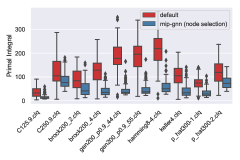
(a) Box plots for the distribution of Primal Integrals for the ten problem sets, each with 100 instances; lower is better.

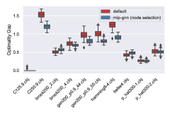
(b) Box plots for the distribution of the Optimality Gaps at termination for all problem sets; lower is better.

(c) Comparison of three GNN architectures with different $\tau$ values used in training on a single GISP problem set; lower primal integral values are better. The performance impact of the threshold depends on the GNN architecture, with a more pronounced effect for the EdgeConvolution architecture (ECS).

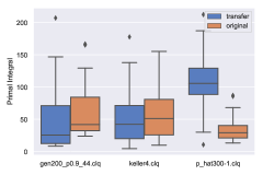
(d) Transfer learning on GISP; Box plots for the distribution of Primal Integrals for three problem sets; lower is better. “original” refers to the performance of a model trained on instances from the same distribution; “transfer” refers to that of a model trained on another distribution.

Figure 2: Generalized Independent Set Problem results.

Experimental Evaluation

Next, we investigate the benefits of using MIP-GNN within a state-of-the-art solver on challenging BLP problems. In this section, we will focus primarily on node selection and to a lesser extent warm-starting. Results on using MIP-GNN to guide variable selection are provided in the appendix. We would like to highlight two key features of our experimental design: (1) We use the CPLEX solver, with all of its advanced features (presolve, cuts, heuristics), both as a backend for our method and as a baseline. As such, our implementation and comparisons to CPLEX closely resemble how hard MIPs are solved in real applications, rather than be confined to less advanced academic solvers or artificial case studies; (2) We evaluate our method on two classes of problems that are simultaneously important for operations research applications and extremely difficult to find good solutions for or solve to optimality. In contrast, we have attempted to apply MIP-GNN to instances provided by Ding et al. (2020) and found them to be extremely easy for CPLEX which solves them to global optimality in seconds on average. Because machine learning is unlikely to substantially reduce such already small running times, we believe that tackling truly challenging tasks, such as those we study here, is where learning holds most promise.

Data collection Given a BLP training instance, the main data collection step is to estimate the variable biases. To do so, we must collect a set of high-quality feasible solutions. We leverage a very useful feature of modern solvers: the solution pool, particularly CPLEX’s implementation. This feature repurposes the solver to collect a large number of good integer solutions, rather than focus on proving optimality. For our dataset, we let CPLEX spend 60 minutes in total to construct this solution pool for each instance, terminating whenever it has found $1000$ solutions with objective values within $10\,\%$ of the best solution found, or when the 60-minute limit is reached. The variable biases are calculated according to Eq. (2).

Neural architecture To implement the two passes of the MIP-GNN described above, we used the GIN-$\varepsilon$ (Xu et al. 2019) (GIN) and GraphSage (Hamilton, Ying, and Leskovec 2017) (Sage) architectures for both passes, with and without error propagation. To deal with continuous edge features, we used a $2$-layer MLP to map them to the same number of components as the node features and combined them using summation. Further, we implemented a variant of EdgeConvolution (Simonovsky and Komodakis 2017) (EC), again with and without error propagation, handling edge features, in a natural way; see the appendix for details. For node features, we only used the corresponding objective function coefficient and node degree for variable nodes, and the right-hand side coefficient (i.e., the corresponding component of $\mathbf{b}$) and the node degree (i.e., the number of nonzeros in the constraint) for constraint nodes. For edge features, we used the corresponding entry in $\mathbf{A}$.

For all architectures, we used mean aggregation and a feature dimension of $64$. Four GNN layers were used, i.e., four interleaved variable-to-constraint and constraint-to-variable passes, followed by a $4$-layer MLP for the final classification.

Benchmark problems The generalized independent set problem (GISP) (Colombi, Mansini, and Savelsbergh 2017) and fixed-charge multi-commodity network flow problem (FCMNF) (Hewitt, Nemhauser, and Savelsbergh 2010) have been used to model a variety of applications including forest harvesting (Hochbaum and Pathria 1997) and supply chain planning, respectively. Importantly, it is straightforward to generate realistic instances of GISP/FCMNF that are extremely difficult to solve or even find good solutions for, even when using a commercial solver such as CPLEX. For each problem set (10 from GISP, 1 from FCMNF), there are 1000 training instances and 100 test instances. These instances have thousands to tens of thousands of variables and constraints, with the GISP problem sets varying in size, as described in Table 2 of (Colombi, Mansini, and Savelsbergh 2017). Appendix section “Data generation” includes additional details.

Baseline solver We use CPLEX 12.10.0 as a backend for data collection and BLP solving. CPLEX “control callbacks” allowed us to integrate the methods described in Section Guiding a Solver with MIP-GNN in the solver. We ask CPLEX to “emphasize feasibility over optimality” by setting its “emphasis switch” parameter appropriately; this setting makes the CPLEX baseline (referred to as “default” in the results section) even more competitive w.r.t. evaluation metrics that emphasize finding good feasible solutions quickly. We allow CPLEX to use presolve, cuts, and primal heuristics regardless of whether it is being controlled by our MIP-GNN models or not. As such, all subsequent comparisons to “default” are to this full-fledged version of CPLEX, rather than to any stripped-down version. We note that this is indeed already a very powerful baseline to compare against, as CPLEX has been developed and tuned over three decades by MIP experts, i.e., it can be considered a very sophisticated human-learned solver. The solver time limit is 30 minutes per instance.

Experimental protocol During training, 20% of the training instances were used as a validation set for early stopping. The training algorithm is Adam (Kingma and Ba 2015), which ran for $30$ epochs with an initial learning rate of $0.001$ and exponential learning rate decay with a patience of $10$. Training is done on GPUs whereas evaluation (including making predictions with trained models and solving MILPs with CPLEX) is done on CPUs with a single thread. Appendix section “CPU/GPU specifications” provides additional details.

Evaluation metrics All subsequent results will be based on test instances that were not seen during any training run. Because MIP-GNN is designed to guide the solver towards good feasible solutions, the widely used “Primal Integral” metric (Berthold 2013) will be adopted, among others, to assess performance compared to the default solver setting. In short, the primal integral can be interpreted as the average solution quality during a time-limited MIP solve. Smaller values indicate that high-quality solutions were found early in the solving process. Quality is relative to a reference objective value; for GISP/FCMNF, it is typically difficult to find the optimal values of the instances, and so we use as a reference the best solution values found by any of the tested methods. We will also measure the optimality gap. Other relevant metrics will be described in the corresponding figure/table.

Results and Discussion

MIP-GNN (node selection) vs. default CPLEX In Figure 2(a), we use box plots to examine the distribution of primal integral values on the ten test problem sets of GISP. Guiding node selection with MIP-GNN predictions (blue) conclusively outperforms the default setting (red) on all test sets. Equally importantly, appendix Table 5 shows that not only is the primal integral better when using MIP-GNN for node selection, but also that the quality of the best solution found at termination improves almost always compared to default. This improvement on the primal side translates into a reduction of the optimality gap for most datasets, as shown in Figure 2(b). Additional GISP statistics/metrics are in the appendix.

As for the FCMNF dataset (detailed results in appendix), MIP-GNN node selection also outperforms CPLEX default, leading to better solutions 81% of test instances (Table 1) and smaller primal integrals on 62% (Table 3).

Appendix figures 6 and 7 shed more light into how MIP-GNN uses affect the solution finding process in the MIP solver. Strategy “node selection” finds more incumbent solutions (Figure 6) than “default”, but also many more of those incumbents are integer solutions to node LP relaxations (Figure 7). This indicates that this guided node selection strategy is moving into more promising reasons of the search tree, which makes incumbents (i.e., improved integer-feasible solutions) more likely to be found by simply solving the node LP relaxations. In contrast, “default” has to rely on solver heuristics to find incumbents, which may incur additional running times.

MIP-GNN (warmstart) vs. default CPLEX Appendix Table 6 shows that warm-starting the solver using MIP-GNN consistently yields better final solutions on 6 out of 9 GISP datasets (with one dataset exhibiting a near-tie); Table 7 shows that the optimality gap is also smaller when warm-starting with our models on 6 out of 9 datasets. This is despite our implementation of warm-starting being quite basic, e.g., the rounding thresholds are examined sequentially rather than in parallel, which means that a non-negligible amount of time is spent during this phase before CPLEX starts branch and bound. We do note, however, that guided node selection seems to be the most suitable use of MIP-GNN predictions.

Transfer learning Does a MIP-GNN model trained on one set still work well on other, slightly different sets from the same optimization problem? Figure 2(d) shows the primal integral box plots (similar to those of Figure 2(a)) on three distinct GISP problem sets, using two models: “original” (orange), trained on instances from the same problem set; “transfer” (blue), trained on a problem set that is different from all the others. On the first two problem sets, the “transfer” model performs as well or better than the “original” model; on the last, “original” is significantly better. Further analysis will be required to determine the transfer potential.

GNN architectures The MIP-GNN results in Figures 2(a) and 2(b) and Table 5 used a Sage architecture with error messages and a threshold of $\tau=0$. Figure 2(c) compares additional GNN architectures with three thresholds on the GISP problem set C250.9.clq (which has the largest number of variables/constraints). The effect of the threshold only affects the EdgeConvolution (ECS) architecture, with zero being the best.

Conclusions

We introduced MIP-GNN, a generic GNN-based architecture to guide heuristic components within state-of-the-art MIP solvers. By leveraging the structural information within the MILP’s constraint-variable interaction, we trained MIP-GNN in a supervised way to predict variable biases, i.e., the likelihood of a variable taking a value of 1 in near-optimal solutions. On a large set of diverse, challenging, real-world BLPs, we showed a consistent improvement over CPLEX’s default setting by guiding node selection without additional feature engineering. Crucially, for the first time in this line of research, we used a single, once-trained model for bias prediction to speed up multiple components of the MIP solver simultaneously. In other words, we showed that learning the bias associated with sets of near-optimal solutions is empirically beneficial to multiple crucial MIP ingredients. We reported in detail the effect on node selection and warm-starting while also showing promising results for variable selection. Further, our framework is extensible to yet other crucial ingredients, e.g., preprocessing, where identifying important variables can be beneficial.

Appendix A Implementation details

Code, data, and pre-trained models can be found at https://github.com/lyeskhalil/mipGNN. See the folder code/ for the source code of all used GNN architectures and evaluation protocols for the downstream tasks, the folder code/gnn_models/pretrained_models/ for pretrained models, and code/README.md on how to reproduce the reported results.

Appendix B Data generation

For GISP, we generate ten problem sets, each corresponding to a different graph that underlies the combinatorial problem; the graphs are from the DIMACS library. The instance generation procedure follows that of (Colombi, Mansini, and Savelsbergh 2017), particularly the hardest subset from that paper, which is referred to as “SET2, $\alpha=0.75$”. For FCMNF, we generate a single problem set based on the procedure described in (Hewitt, Nemhauser, and Savelsbergh 2010). Table 10 includes statistics on the number of variables and constraints in each of the datasets.

Appendix C CPU/GPU specifications

All neural architectures were trained on a workstation with two Nvidia Tesla V100 GPU cards with 32GB of GPU memory running Oracle Linux Server 7.7. Training a model took between 15 and 40 minutes depending on the size of the datasets/instances, including inference times on test and validation sets.

When using the trained models within CPLEX, inference is done on CPU and accounted for in all time-based evaluation metrics. For CPU-based computations (data collection and MILP solving), we used a cluster with 32-core machines (Intel E5-2683 v4) and 125GB memory. Individual data collection or BLP solving tasks were single-threaded, though we parallelized distinct tasks.

Appendix D Guiding branching variable selection with MIP-GNN predictions

As discussed, using MIP-GNN’s bias predictions to guide node selection we aim at finding good feasible solutions quickly. Another way of using these predictions is to guide the variable selection strategy of the solver. This can be achieved by asking the solver to prioritize branching on variables whose bias prediction is close to 0 or 1. Formally, we provide the solver with priority scores for each binary variable, computed as $\texttt{score}(\widehat{\mathbf{p}}_{i})$, the confidence score defined earlier in this section. Then, given a node $N$ with a set $C(N)$ of candidates for branching (namely, the variables with fractional values in the node relaxation solution), the solver branches on $x_{i}\coloneqq\arg\max_{i\in C(N)}\{\texttt{score}(\widehat{\mathbf{p}}_{i})\}$.

Note that the node selection and branching cases use the predicted bias in a complementary way: for node selection, we look at the variables already fixed, while, for variable selection, we look at those yet to be fixed.

Appendix E Extension to ILP and MILP

While we described the MIP-GNN as an architecture for BLPs, it applies to general ILPs as well. That is, we can transform a given ILP instance into a BLP through a binary expansion of each integer (non-binary) variable $x_{i}$ by assuming an upper bound $U_{i}$ on it is known or it can be computed (as it is generally the case). This clearly requires the addition of $\lceil\log_{2}U_{i}\rceil+1$ binary variables, which can lead to a large BLP if the $U_{i}$’s are big. Alternatively, we can stick to the given ILP formulation and treat the learning problem as a multi-class instead of a binary classification problem.

Finally, in the presence of continuous variables, i.e., either MILPs or mixed-binary linear programs, we ignore them and compute the bias only for the integer-constrained variables by assuming that the optimal value of the continuous variables can be computed a posteriori by simpling solving an LP (i.e., after fixing the integer variables to their predicted values).

Appendix F Details on GNN architectures

As outlined in the main paper, we used the GIN-$\varepsilon$ (GIN) (Xu et al. 2019), GraphSage (Hamilton, Ying, and Leskovec 2017), with and without error propagation, to express $f^{\vec{W_{2,X}}}_{\text{merge}}$ and $f^{\vec{W_{1,X}}}_{\text{aggr}}$ for $\vec{X}$ in $\{\vec{C},\vec{V}\}$. To deal with continuous edge features, we used a $2$-layer MLP to map them to the same number of components as the node features and combined them using summation. Further, we implemented a variant of EdgeConvolution (EC) (Simonovsky and Komodakis 2017), that can handle continuous edge feature in a natural way. That is, a feature $\vec{v}_{i}^{(t+1)}$ (c-to-v pass) for variable node $v_{i}$ is computed as

$$\sum_{j\in\mathcal{N}(i)}h([\vec{v}_{i}^{(t)},\vec{c}_{j}^{(t)},A_{ji},b_{j},e_{j}]),$$

where $h$ is a $2$-layer MLP. The v-to-c pass is computed in an analogous fashion.

Appendix G Theoretical guarantees

In the following, we show that, under certain assumptions, GNNs are, in principle, capable of outputting feasible solutions of the relaxation of the underlying BLPs, minimizing the MAE to (real-valued) biases on a given (finite) training set. We do so by leveraging a connection to the multiplicative weights update algorithm (MWU), e.g., see (Arora, Hazan, and Kale 2012) for a thorough overview.

Given a BLP $I=(\vec{A},\vec{b},\vec{c})$, its corresponding relaxation $\widehat{I}$, and $\varepsilon>0$, a vector $\vec{x}_{\varepsilon}$ in $\mathbb{R}^{n}$ is a $\varepsilon$-feasible solution for the relaxation $\widehat{I}$ if

$$\vec{A}\vec{x}_{\varepsilon}\geq\vec{b}-\vec{1}\varepsilon$$

holds. That is, an $\varepsilon$-feasible solution violates each constraint of $\widehat{I}$ by at most $\varepsilon$.

Let $\vec{a}$ in $\mathbb{R}^{n}$ and $b$ in $\mathbb{R}$, then we assume, following, e.g., (Arora, Hazan, and Kale 2012), that there exists an oracle $\mathcal{O}$ either returning $\vec{x}\geq 0$ satisfying $\vec{a}^{\mathsf{T}}\vec{x}\geq b$ or determining that the system is not feasible. Put differently, we assume that we have access to an oracle $\mathcal{O}$ that outputs a feasible solution $\vec{x}\geq 0$ to a linear system with one inequality, i.e., $\vec{p}^{\mathsf{T}}\vec{A}\vec{x}\geq\vec{p}^{\mathsf{T}}\vec{b}$, where the vector $\vec{p}$ is from the $(n+1)$-dimensional probability simplex. Again following, e.g., (Arora, Hazan, and Kale 2012), we assume that for any $\vec{x}$ in $\mathbb{R}^{n}$ the oracle ${\mathcal{O}}$ outputs it holds that

$$\vec{A}_{j}\vec{x}-b_{j}\in[-\rho,\rho]$$

for some $\rho>0$ and $j$ in $[m]$, resulting in the following assumption.

Assumption 1.

There exists a neural unit simulating the oracle $\mathcal{O}$, i.e., returning the same results as the oracle $\mathcal{O}$, given the same input.

Although this assumption is rather strict, such oracle can be expressed by standard neural architectures, see, e.g., (Pérez, Marinkovic, and Barceló 2019). Further, given a BLP $I$ or a finite set of BLP, we assume an upper-bound of $\Delta\cdot n>0$ on the minimum $\ell_{1}$ distance between a feasible point of the relaxation $\widehat{I}$ and the bias vector $\vec{\bar{b}}(I)$ of the BLP $I$.

Assumption 2.

Given a BLP $I=(\vec{A},\vec{b},\vec{c})$ with bias $\vec{\bar{b}}(I)$ and corresponding relaxation $\widehat{I}$, there exists a $\Delta>0$ such that

$$\min_{\vec{x}\in F(\hat{I})}\lVert\vec{x}-\vec{\bar{b}}(I)\rVert_{1}\leq\Delta\cdot n.$$

For a set of BLP $S$, we assume

$$\sum_{I\in S}\min_{\vec{x}\in F(\hat{I})}\lVert\vec{x}-\vec{\bar{b}}(I)\rVert_{1}\leq\Delta\cdot\sum_{I\in S}n_{i},$$

where $n_{i}$ denotes the number of variables of instance $I_{i}$.

Now the following result states that there exists a GNN architecture and corresponding weight assignments that outputs $\varepsilon$-feasible solutions for the relaxations of MILPs from a finite (training) set, minimizing the MAE to (real-valued) bias predictions.

Proposition 1.

Let $S=\{(I_{i},\vec{\bar{b}}(I_{i}))\}_{i\in[|S|]}$ be a finite training set of (feasible) MILPs with corresponding biases and let $\varepsilon>0$. Then, under Assumption 1 and 2, there exists a GNN architecture and corresponding weights such that it outputs an $\varepsilon$-feasible solution $\vec{\widehat{x}}_{I_{i}}$ for the relaxation of each MILP $I_{i}$ in $S$ and

$$\nicefrac{{1}}{{|S|}}\sum_{I_{i}\in S}\nicefrac{{1}}{{n_{i}}}\lVert\vec{\widehat{x}}_{I_{i}}-\vec{\bar{b}}(I_{i})\rVert_{1}\leq\varepsilon+\Delta,$$

upper-bounding the MAE on the training set $S$. Here, $n_{i}$ denotes the number of variables of instance $I_{i}$. The number of layers of the GNN is polynomially-bounded in $\varepsilon$ and logarithmically-bounded in the number of constraints over all instances.

Proof sketch.

Without loss of generality, we can encode the $S$ relaxations $\widehat{I}_{i\in[|S|]}$ as one LP with a sparse, block-diagonal constraint matrix. Henceforth, we just focus on a single instance/bias pair $(I,\bar{\vec{b}})$ in $S$ with $I=(\vec{A},\vec{b},\vec{c})$. Now consider the following (convex) optimization problem:

$$\arg\min_{\vec{x}}\lVert\vec{x}-\vec{\bar{b}}\rVert_{1}$$ (L1)

$$\vec{A}\vec{x}\geq\vec{b}.$$

Since, by assumption, $\lVert\vec{x}-\vec{\bar{b}}\rVert_{1}=\sum_{i=1}^{n}|x_{i}-\vec{\bar{b}}_{i}|\leq\Delta\cdot n$, each summand, “on average”, introduces an error of $\Delta$. Hence, we can transform the optimization problem L1, using a standard transformation, into a system of linear inequalities (System L2). Since system L2 is feasible by construction, the MWU algorithm will return an $\varepsilon$-feasible solution $\vec{\widehat{x}}$ for L2 and the relaxation $\widehat{I}$, see Theorem 2. By stitching everything together, we get

$$\lVert\vec{\widehat{x}}-\vec{\bar{b}}\rVert_{1}\leq(\Delta+\varepsilon)\cdot n.$$

Hence, on average over $n$ variables, we introduce an error of $\varepsilon+\Delta$. This finishes the part of the proof upperbounding the MAE.

We now show how to simulate the MWU via a GNN. First, observe that we can straightforwardly interpret the MWU algorithm as a message-passing algorithm, as outlined in Algorithm 1. Since every step can be expressed as a summation or averaging over neighboring nodes on a suitably defined graph, encoding the system L2 for all $S$ relaxations $\widehat{I}_{i\in[|S|]}$, there exists an implementation of the functions $f^{t,\vec{W_{1}}}_{\text{aggr}}$ and $f^{t,\vec{W_{2}}}_{\text{merge}}$ of Equation 1 and corresponding parameter initializations such that we can (exactly) simulate each iteration $t$ of the MWU in $\mathbb{R}^{d}$ for some suitable chosen $d>0$, depending linearly on $|S|$ and $n$. By the same reasoning, there exists an MLP that maps each such encoded variable assignment for variable $x_{i}$ onto the solution $\nicefrac{{\bar{x}_{i}}}{{T}}$ returned by Algorithm 1. The bound on the number of required GNN layers is a straightforward application of Theorem 2.∎

Input: Bipartite constraint graph $B(I)$, $\varepsilon>0$, stepsize $\eta>0$, scaling constant $\rho$.
Output: $\varepsilon$-feasible $\vec{\bar{x}}$ or non-feasible.

1:Initialize weights $w_{j}\leftarrow 1$ for each constraint node

2:Initialize probabilities $p_{j}\leftarrow\nicefrac{{1}}{{m}}$ for each constraint node

3:Set $T$ to according Equation 3

4:for $t\text{ in }[T]$ do

5:     Update each variable node $\vec{v}_{i}$ based on output $\vec{x}_{i}$ of oracle $\mathcal{O}$ using $\vec{p}$

6:     Compute error signal ${e}_{i}$ for each constraint node $\vec{c}_{j}$

$$e_{j}\leftarrow\nicefrac{{1}}{{\rho}}\,\Big{(}\sum_{i\in N(j)}A_{ji}\vec{x}_{i}\Big{)}-\vec{b}_{j}$$

7:     Update $w_{i}\leftarrow(1-\eta e_{j})w_{i}$

8:     Normalize weights $p_{j}\leftarrow\nicefrac{{w_{j}}}{{\boldsymbol{\Gamma}(t)}}$ for $i$ in $[m]$, where $\boldsymbol{\Gamma}(t)=\sum_{i\in[m]}\vec{w}_{i}$

9:     Update solution $\vec{\bar{x}}\leftarrow\vec{\bar{x}}+\vec{x}$

10:end for

11:return Average over solutions $\nicefrac{{\vec{\bar{x}}}}{{T}}$

Algorithm 1 MWU (Message passing version) for the LP feasibility problem.

Theorem 2 (E.g., (Arora, Hazan, and Kale 2012)).

Given a BLP $I=(\vec{A},\vec{b},\vec{c})$, its corresponding relaxation $\widehat{I}$, and $\varepsilon>0$, Algorithm 1 with

$$T=\left\lceil\frac{4\rho\ln(m)}{\varepsilon^{2}}\right\rceil,$$ (3)

outputs an $\varepsilon$-feasible solution for $\widehat{I}$ or determines that $\widehat{I}$ is not feasible.

Appendix H Additional experimental results – FCMNF

Here, we report on additional results for the FCMNF dataset. In summary, while the improvements due to guiding the solver with MIP-GNN predictions are more pronounced for GISP, they are also statistically significant for FCMNF.

• Table 1 shows that MIP-GNN node selection leads to better solutions than the default solver on 81/100 test instances of this problem.

• Similarly, Table 3 shows that the primal integral is smaller (better) most of the time (62/100 wins). Table 3 shows that the primal integral is also smaller on average and w.r.t. the median.

• Figures 3(a) and 3(b) are analogous to GISP Figures 2(a) and 2(b) from the main text.

Table 1: FCMNF; number of wins, ties, and losses, for the proposed method (MIP-GNN for node selection), with respect to the objective value of the best solution found compared to the default solver setting.

Problem Set	Wins	Ties	Losses	p-value
L_n200_p0.02_c500	81	0	17	5.18129e-14

Table 2: FCMNF; number of wins, ties, and losses, for the proposed method (MIP-GNN for node selection), with respect to the Primal Integral compared to the default solver setting.

Problem Set	Wins	Ties	Losses	p-value
L_n200_p0.02_c500	62	0	36	0.015951

Table 3: FCMNF; statistics on the Primal Integral for the one problem sets with 100 instances; lower is better.

Problem Set	Method	Statistics
		Avg.	Std.	Median
L_n200_p0.02_c500	default	137.05	49.74	133.46
	MIP-GNN (node selection)	125.97	34.14	122.49

Table 4: FCMNF; statistics on the Optimality Gap for the one problem sets with 100 instances; lower is better.

Problem Set	Method	Statistics
		Avg.	Std.	Median
L_n200_p0.02_c500	default	0.33	0.03	0.33
	MIP-GNN (node selection)	0.35	0.03	0.34

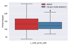
(a) Box plots for the distribution of Primal Integrals for the ten problem sets, each with 100 instances; lower is better.

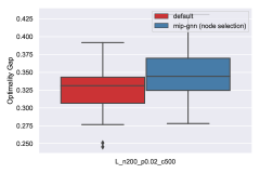
(b) Fixed-Charge Multi-Commodity Network Flow (FCMNF); Box plots for the distribution of Optimality Gaps for the ten problem sets, each with 100 instances; lower is better.

Figure 3: Fixed-Charge Multi-Commodity Network Flow (FCMNF); distribution of Primal Integrals and Optimality Gaps.

Appendix I Additional experimental results – GISP

Here, we report on additional results for the GISP datasets.

• Table 5 shows that the proposed method (MIP-GNN for node selection) finds a better final solution than default CPLEX. This complements the results in the main text, which show improvements w.r.t. the primal integral.

• Tables 8 and 9 show statistics for the primal integral and the optimality gap, respectively, for both the default solver and three uses of the MIP-GNN models.

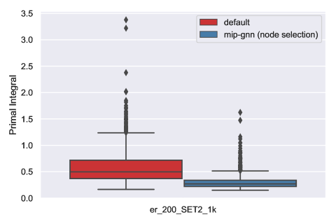
Figure 8: Box plots for the distribution of Primal Integrals for the Erdos-Renyi test dataset with 1000 instances; lower is better.

• Figures 8 and Figure 5 extend Figure 2(a) and Figure 2(b) from the main text to include the two other uses of MIP-GNN, “variable selection” and “warmstart”. While “variable selection” sometimes outperforms “default”, “node selection” is typically the winner.

• Figures 6 and 7 shed more light into how MIP-GNN uses affect the solution finding process in the MIP solver. “node selection” finds more incumbent solutions (Figure 6) than “default”, but also many more of those incumbents are integer solutions to node LP relaxations (Figure 7). This indicates that this guided node selection strategy is moving into more promising reasons of the search tree, which makes incumbents (i.e., improved integer-feasible solutions) more likely to be found by simply solving the node LP relaxations. In contrast, “default” has to rely on solver heuristics to find incumbents, which may incur additional running time costs.

Table 5: Generalized Independent Set Problem; number of wins, ties, and losses, for MIP-GNN (node selection), with respect to the objective value of the best solution found compared to the default solver setting. Column “p-value” refers to the result of the Wilcoxon signed-rank test; smaller values indicate that our method is better than default.

Problem Set	Wins	Ties	Losses	p-value
C125.9	2	98	0	0.08
C250.9	89	1	10	2.3e-16
brock200_2	75	1	24	3.4e-08
brock200_4	87	3	10	2.2e-15
gen200_p0.9_44	97	0	3	3.5e-18
gen200_p0.9_55	99	0	1	2.7e-18
hamming8-4	98	0	2	2.3e-18
keller4	84	1	15	8.7e-13
p_hat300-1	86	0	14	2.7e-14
p_hat300-2	87	0	13	1e-15

Table 6: Generalized Independent Set Problem; number of wins, ties, and losses, for MIP-GNN (warmstart), with respect to the objective value of the best solution found compared to the default solver setting. Column “p-value” refers to the result of the Wilcoxon signed-rank test; smaller values indicate that our method is better than default.

Problem Set	Wins	Ties	Losses	p-value
C125.9.clq	2	98	0	0.09
C250.9.clq	52	25	23	2e-05
brock200_2.clq	42	6	52	0.96
brock200_4.clq	14	77	9	0.17
gen200_p0.9_44.clq	43	22	35	0.18
gen200_p0.9_55.clq	67	14	19	1.8e-07
hamming8-4.clq	62	14	24	1.3e-07
keller4.clq	36	47	17	5e-03
p_hat300-1.clq	89	0	11	9.8e-15
p_hat300-2.clq	87	0	13	1.2e-14

Table 7: Generalized Independent Set Problem; number of wins, ties, and losses, for MIP-GNN (warmstart), with respect to the optimality gap compared to the default solver setting. Column “p-value” refers to the result of the Wilcoxon signed-rank test; smaller values indicate that our method is better than default.

Problem Set	Wins	Ties	Losses	p-value
C125.9.clq	4	96	0	0.03
C250.9.clq	59	17	24	5.4e-06
brock200_2.clq	25	0	75	1
brock200_4.clq	32	37	31	0.2
gen200_p0.9_44.clq	47	4	49	0.23
gen200_p0.9_55.clq	80	1	19	3.2e-10
hamming8-4.clq	75	6	19	1.6e-10
keller4.clq	65	9	26	7.6e-06
p_hat300-1.clq	96	0	4	4.1e-17
p_hat300-2.clq	67	0	33	3e-06

Figure 4: Generalized Independent Set Problem; Box plots for the distribution of Primal Integrals for the ten problem sets, each with 100 instances; lower is better.

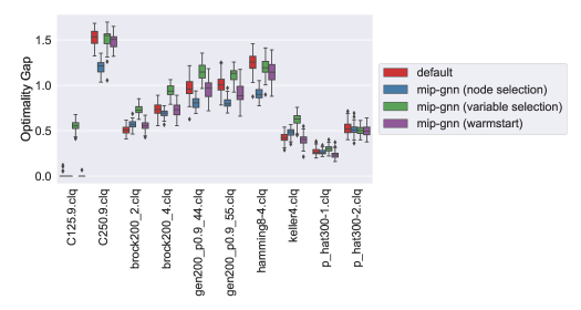
Figure 5: Generalized Independent Set Problem; box plots for the distribution of Optimality Gaps for the ten problem sets, each with 100 instances; lower is better.

Figure 6: Generalized Independent Set Problem; box plots for the distribution of the number of solutions found during branch and bound for the ten problem sets, each with 100 instances.

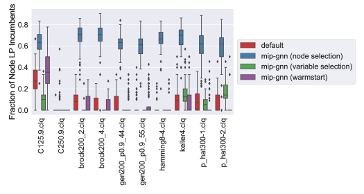
Figure 7: Generalized Independent Set Problem; box plots for the distribution of the number of solutions found during branch and bound by solving the LP relaxation at a node of the search tree; each boxplot corresponds to on of the ten problem sets, each with 100 instances.

Table 8: Generalized Independent Set Problem; statistics on the Primal Integral for the ten problem sets, each with 100 instances; lower is better.

Problem Set	Method	Statistics
		Avg.	Std.	Median
C125.9.clq	default	34.19	20.78	31.85
	MIP-GNN (node selection)	14.90	9.76	11.13
	MIP-GNN (variable selection)	89.55	50.28	91.07
	MIP-GNN (warmstart)	30.73	18.87	29.85
C250.9.clq	default	129.32	72.61	109.21
	MIP-GNN (node selection)	96.31	42.92	86.54
	MIP-GNN (variable selection)	116.01	67.90	99.63
	MIP-GNN (warmstart)	200.62	65.49	195.52
brock200_2.clq	default	96.95	43.53	95.58
	MIP-GNN (node selection)	59.22	34.82	52.44
	MIP-GNN (variable selection)	89.95	55.09	89.55
	MIP-GNN (warmstart)	214.25	40.62	213.43
brock200_4.clq	default	130.17	52.64	132.57
	MIP-GNN (node selection)	44.49	24.60	35.67
	MIP-GNN (variable selection)	128.70	49.62	128.40
	MIP-GNN (warmstart)	166.68	52.80	170.40
gen200_p0.9_44.clq	default	181.35	65.72	182.17
	MIP-GNN (node selection)	43.75	23.18	34.98
	MIP-GNN (variable selection)	165.85	63.93	163.84
	MIP-GNN (warmstart)	239.93	68.44	243.68
gen200_p0.9_55.clq	default	186.81	63.17	198.87
	MIP-GNN (node selection)	50.97	28.25	38.78
	MIP-GNN (variable selection)	148.54	56.96	160.39
	MIP-GNN (warmstart)	184.92	59.18	189.92
hamming8-4.clq	default	220.08	66.47	222.97
	MIP-GNN (node selection)	65.05	36.29	52.95
	MIP-GNN (variable selection)	173.04	66.91	169.89
	MIP-GNN (warmstart)	248.14	63.11	253.16
keller4.clq	default	107.92	43.92	111.63
	MIP-GNN (node selection)	46.99	29.44	40.66
	MIP-GNN (variable selection)	90.94	46.81	85.39
	MIP-GNN (warmstart)	99.43	50.20	101.27
p_hat300-1.clq	default	83.62	24.00	83.06
	MIP-GNN (node selection)	43.05	22.48	37.97
	MIP-GNN (variable selection)	41.86	21.70	37.60
	MIP-GNN (warmstart)	44.95	31.08	33.41
p_hat300-2.clq	default	139.69	43.99	143.98
	MIP-GNN (node selection)	96.26	36.65	91.61
	MIP-GNN (variable selection)	62.58	34.09	56.30
	MIP-GNN (warmstart)	117.24	44.95	108.24

Table 9: Generalized Independent Set Problem; statistics on the Optimality Gap for the ten problem sets, each with 100 instances; lower is better. The gap is calculated at solver termination with a time limit of 30 minutes per instance. A gap of zero indicates that an instance has been solved to proven optimality. For GISP, this only happens for (most methods and most instances of) C125.9.clq, the problem set with the smallest number of variables and constraints. For other problem sets, most instances time out with relatively large gaps. A gap of $0.4$, for example, can be interpreted as: the best solution found at termination is guaranteed to be with in $40\%$ of optimal. The optimality gap is calculated by CPLEX as $\nicefrac{{|\text{bestbound}-\text{bestinteger}|}}{{(10^{-9}+|\text{bestinteger}|)}}$.

Problem Set	Method	Statistics
		Avg.	Std.	Median
C125.9.clq	default	0.00	0.02	0.00
	MIP-GNN (node selection)	0.00	0.00	0.00
	MIP-GNN (variable selection)	0.55	0.06	0.55
	MIP-GNN (warmstart)	0.00	0.01	0.00
C250.9.clq	default	1.53	0.09	1.53
	MIP-GNN (node selection)	1.21	0.07	1.21
	MIP-GNN (variable selection)	1.52	0.10	1.55
	MIP-GNN (warmstart)	1.48	0.08	1.50
brock200_2.clq	default	0.51	0.05	0.51
	MIP-GNN (node selection)	0.57	0.04	0.57
	MIP-GNN (variable selection)	0.73	0.05	0.73
	MIP-GNN (warmstart)	0.56	0.05	0.56
brock200_4.clq	default	0.73	0.07	0.73
	MIP-GNN (node selection)	0.69	0.04	0.69
	MIP-GNN (variable selection)	0.94	0.06	0.94
	MIP-GNN (warmstart)	0.73	0.07	0.73
gen200_p0.9_44.clq	default	0.97	0.10	0.96
	MIP-GNN (node selection)	0.81	0.06	0.81
	MIP-GNN (variable selection)	1.15	0.08	1.15
	MIP-GNN (warmstart)	0.96	0.10	0.97
gen200_p0.9_55.clq	default	1.01	0.10	1.01
	MIP-GNN (node selection)	0.81	0.05	0.80
	MIP-GNN (variable selection)	1.12	0.07	1.13
	MIP-GNN (warmstart)	0.91	0.10	0.89
hamming8-4.clq	default	1.25	0.10	1.26
	MIP-GNN (node selection)	0.91	0.06	0.90
	MIP-GNN (variable selection)	1.20	0.10	1.19
	MIP-GNN (warmstart)	1.15	0.11	1.14
keller4.clq	default	0.42	0.05	0.42
	MIP-GNN (node selection)	0.48	0.04	0.49
	MIP-GNN (variable selection)	0.62	0.07	0.63
	MIP-GNN (warmstart)	0.40	0.06	0.40
p_hat300-1.clq	default	0.27	0.04	0.26
	MIP-GNN (node selection)	0.26	0.03	0.26
	MIP-GNN (variable selection)	0.30	0.03	0.30
	MIP-GNN (warmstart)	0.23	0.04	0.23
p_hat300-2.clq	default	0.53	0.06	0.52
	MIP-GNN (node selection)	0.51	0.05	0.51
	MIP-GNN (variable selection)	0.50	0.05	0.50
	MIP-GNN (warmstart)	0.50	0.06	0.49

Table 10: Training dataset statistics.

Problem Set	Num. graphs	Avg. num. variables	Avg. num. constraints	Avg. non-zeros in constraints
p_hat300-2.clq	1 000	16 748.8	21 928.0	120 609.6
gisp_C250.9.clq	1 000	21 239.5	27 984.0	153 915.0
keller4.clq	1 000	7 247.6	9 435.0	51 893.3
hamming8-4.clq	1 000	15 906.6	20 864.0	114 757.1
gen200_p0.9_55.clq	1 000	13 634.5	17 910.0	98 508.9
gen200_p0.9_44.clq	1 000	13 643.8	17 910.0	98 527.5
C125.9.clq	1 000	5 347.9	6 963.0	38 297.9
p_hat300-1.clq	1 000	8 501.1	10 933.0	60 134.1
brock200_4.clq	1 000	10 018.5	13 089.0	71 993.1
brock200_2.clq	1 000	7 607.9	9 876.0	54 319.8
L_n200_p0.02_c500	1 000	80 497.0	20 797.0	479 794.0

Appendix J Additional Experimental Results – GISP on Erdos-Renyi Graphs

We also performed experiments on GISP instances based on synthetic Erdos-Renyi graphs. Contrary to other datasets, each generated instance is based on a different randomly generated Erdos-Renyi graph on 200 nodes, with the number of edges ranging between 1 867 and 2 136; the Erdos-Renyi graph generator has an edge probability of 0.1, and so the expected number of edges is roughly 2 000. As in the other GISP graphs used in the paper, the set of removable edges is also random with the same probability of inclusion in the set, $\alpha=0.75$.

Of note is the fact that these instances are generally easier to solve to optimality than other datasets considered in this work. As such, the solver time limit is reduced to 10 minutes. Also, the room for improvement in metrics of interest such as the Primal Integral is smaller. Coupled with the fact that each GISP instance has a different underlying random graph, makes improving over default CPLEX a challenging task for our method.

On 956 out of 1 000 unseen test instances from this alternative distribution, MIP-GNN (node selection) produces a smaller primal integral than default CPLEX; the average primal integral is halved using MIP-GNN (node selection).

Table 11: GISP on Erdos-Renyi graphs; number of wins, ties, and losses, for MIP-GNN (node selection), with respect to the Primal Integral compared to the default solver setting.

Problem Set	Wins	Ties	Losses	p-value
er_200_SET2_1k	956	0	44	3e-157

References

- Arora, Hazan, and Kale (2012) Arora, S.; Hazan, E.; and Kale, S. 2012. The Multiplicative Weights Update Method: a Meta-Algorithm and Applications. Theory Computation, 8(1): 121–164.
- Baskin, Palyulin, and Zefirov (1997) Baskin, I. I.; Palyulin, V. A.; and Zefirov, N. S. 1997. A Neural Device for Searching Direct Correlations between Structures and Properties of Chemical Compounds. Journal of Chemical Information and Computer Sciences, 37(4): 715–721.
- Battaglia et al. (2018) Battaglia, P. W.; Hamrick, J. B.; Bapst, V.; Sanchez-Gonzalez, A.; Zambaldi, V. F.; Malinowski, M.; Tacchetti, A.; Raposo, D.; Santoro, A.; Faulkner, R.; Gülçehre, Ç.; Song, H. F.; Ballard, A. J.; Gilmer, J.; Dahl, G. E.; Vaswani, A.; Allen, K. R.; Nash, C.; Langston, V.; Dyer, C.; Heess, N.; Wierstra, D.; Kohli, P.; Botvinick, M.; Vinyals, O.; Li, Y.; and Pascanu, R. 2018. Relational inductive biases, deep learning, and graph networks. CoRR, abs/1806.01261.
- Bengio et al. (2020) Bengio, Y.; Frejinger, E.; Lodi, A.; Patel, R.; and Sankaranarayanan, S. 2020. A Learning-Based Algorithm to Quickly Compute Good Primal Solutions for Stochastic Integer Programs. In International Conference on Integration of Constraint Programming, Artificial Intelligence, and Operations Research, 99–111.
- Bengio, Lodi, and Prouvost (2021) Bengio, Y.; Lodi, A.; and Prouvost, A. 2021. Machine learning for combinatorial optimization: A methodological tour d’horizon. European Journal of Operational Research, 290(2): 405–421.
- Berthold (2013) Berthold, T. 2013. Measuring the impact of primal heuristics. Operations Research Letters, 41(6): 611–614.
- Bertsimas and Tsitsiklis (1997) Bertsimas, D.; and Tsitsiklis, J. 1997. Introduction to linear optimization. Athena Scientific.
- Bertsimas and Weismantel (2005) Bertsimas, D.; and Weismantel, R. 2005. Optimization over integers. Athena Scientific.
- Bresson and Laurent (2017) Bresson, X.; and Laurent, T. 2017. Residual gated graph convnets. CoRR, abs/1711.07553.
- Bruna et al. (2014) Bruna, J.; Zaremba, W.; Szlam, A.; and LeCun, Y. 2014. Spectral Networks and Deep Locally Connected Networks on Graphs. In ICLR.
- Cappart et al. (2021) Cappart, Q.; Chételat, D.; Khalil, E. B.; Lodi, A.; Morris, C.; and Velickovic, P. 2021. Combinatorial optimization and reasoning with graph neural networks. CoRR, abs/2102.09544.
- Chami et al. (2020) Chami, I.; Abu-El-Haija, S.; Perozzi, B.; Ré, C.; and Murphy, K. 2020. Machine Learning on Graphs: A Model and Comprehensive Taxonomy. CoRR, abs/2005.03675.
- Chen et al. (2019) Chen, Z.; Villar, S.; Chen, L.; and Bruna, J. 2019. On the equivalence between graph isomorphism testing and function approximation with GNNs. In NeurIPS, 15868–15876.
- Chmiela et al. (2021) Chmiela, A.; Khalil, E.; Gleixner, A.; Lodi, A.; and Pokutta, S. 2021. Learning to Schedule Heuristics in Branch and Bound. Advances in Neural Information Processing Systems, 34.
- Colombi, Mansini, and Savelsbergh (2017) Colombi, M.; Mansini, R.; and Savelsbergh, M. 2017. The generalized independent set problem: Polyhedral analysis and solution approaches. European Journal of Operational Research, 260(1): 41–55.
- Dai et al. (2017) Dai, H.; Khalil, E. B.; Zhang, Y.; Dilkina, B.; and Song, L. 2017. Learning combinatorial optimization algorithms over graphs. In NeurIPS, 6351–6361.
- Danna et al. (2007) Danna, E.; Fenelon, M.; Gu, Z.; and Wunderling, R. 2007. Generating multiple solutions for mixed integer programming problems. In International Conference on Integer Programming and Combinatorial Optimization, 280–294. Springer.
- Defferrard, Bresson, and Vandergheynst (2016) Defferrard, M.; Bresson, X.; and Vandergheynst, P. 2016. Convolutional Neural Networks on Graphs with Fast Localized Spectral Filtering. In NeurIPS, 3844–3852.
- Ding et al. (2020) Ding, J.-Y.; Zhang, C.; Shen, L.; Li, S.; Wang, B.; Xu, Y.; and Song, L. 2020. Accelerating Primal Solution Findings for Mixed Integer Programs Based on Solution Prediction. In AAAI Conference on Artificial Intelligence.
- Duvenaud et al. (2015) Duvenaud, D. K.; Maclaurin, D.; Iparraguirre, J.; Bombarell, R.; Hirzel, T.; Aspuru-Guzik, A.; and Adams, R. P. 2015. Convolutional Networks on Graphs for Learning Molecular Fingerprints. In NeurIPS, 2224–2232.
- Fey et al. (2020) Fey, M.; Lenssen, J. E.; Morris, C.; Masci, J.; and Kriege, N. M. 2020. Deep Graph Matching Consensus. In ICLR.
- Fischetti and Lodi (2003) Fischetti, M.; and Lodi, A. 2003. Local branching. Mathematical Programming, 98(1-3): 23–47.
- Gamrath et al. (2020) Gamrath, G.; Anderson, D.; Bestuzheva, K.; Chen, W.-K.; Eifler, L.; Gasse, M.; Gemander, P.; Gleixner, A.; Gottwald, L.; Halbig, K.; Hendel, G.; Hojny, C.; Koch, T.; Le Bodic, P.; Maher, S. J.; Matter, F.; Miltenberger, M.; Mühmer, E.; Müller, B.; Pfetsch, M. E.; Schlösser, F.; Serrano, F.; Shinano, Y.; Tawfik, C.; Vigerske, S.; Wegscheider, F.; Weninger, D.; and Witzig, J. 2020. The SCIP Optimization Suite 7.0. ZIB-Report 20-10, Zuse Institute Berlin.
- Gasse et al. (2019) Gasse, M.; Chételat, D.; Ferroni, N.; Charlin, L.; and Lodi, A. 2019. Exact Combinatorial Optimization with Graph Convolutional Neural Networks. In NeurIPS, 15554–15566.
- Gilmer et al. (2017) Gilmer, J.; Schoenholz, S. S.; Riley, P. F.; Vinyals, O.; and Dahl, G. E. 2017. Neural Message Passing for Quantum Chemistry. In ICML.
- Gupta et al. (2020) Gupta, P.; Gasse, M.; Khalil, E. B.; Kumar, M. P.; Lodi, A.; and Bengio, Y. 2020. Hybrid Models for Learning to Branch. CoRR, abs/2006.15212.
- Gurobi Optimization (2021) Gurobi Optimization, L. 2021. Gurobi Optimizer Reference Manual.
- Hamilton, Ying, and Leskovec (2017) Hamilton, W. L.; Ying, R.; and Leskovec, J. 2017. Inductive Representation Learning on Large Graphs. In NeurIPS, 1025–1035.
- Hewitt, Nemhauser, and Savelsbergh (2010) Hewitt, M.; Nemhauser, G. L.; and Savelsbergh, M. W. 2010. Combining exact and heuristic approaches for the capacitated fixed-charge network flow problem. INFORMS Journal on Computing, 22(2): 314–325.
- Hochbaum and Pathria (1997) Hochbaum, D. S.; and Pathria, A. 1997. Forest harvesting and minimum cuts: a new approach to handling spatial constraints. Forest Science, 43(4): 544–554.
- Hsu et al. (2008) Hsu, E. I.; Muise, C. J.; Beck, J. C.; and McIlraith, S. A. 2008. Probabilistically estimating backbones and variable bias: Experimental overview. In International Conference on Principles and Practice of Constraint Programming, 613–617. Springer.
- IBM (2020) IBM. 2020. CPLEX User’s Manual, Version 12.10.0.
- Joshi, Laurent, and Bresson (2019) Joshi, C. K.; Laurent, T.; and Bresson, X. 2019. An Efficient Graph Convolutional Network Technique for the Travelling Salesman Problem. CoRR, abs/1906.01227.
- Karalias and Loukas (2020) Karalias, N.; and Loukas, A. 2020. Erdos Goes Neural: an Unsupervised Learning Framework for Combinatorial Optimization on Graphs. In NeurIPS.
- Khalil et al. (2016) Khalil, E. B.; Bodic, P. L.; Song, L.; Nemhauser, G. L.; and Dilkina, B. 2016. Learning to Branch in Mixed Integer Programming. In AAAI Conference on Artificial Intelligence, 724–731.
- Khalil et al. (2017) Khalil, E. B.; Dilkina, B.; Nemhauser, G. L.; Ahmed, S.; and Shao, Y. 2017. Learning to Run Heuristics in Tree Search. In Proceedings of the Twenty-Sixth International Joint Conference on Artificial Intelligence, 659–666.
- Kingma and Ba (2015) Kingma, D. P.; and Ba, J. 2015. Adam: A Method for Stochastic Optimization. In ICLR.
- Kipf and Welling (2017) Kipf, T. N.; and Welling, M. 2017. Semi-Supervised Classification with Graph Convolutional Networks. In International Conference on Learning Representation.
- Kireev (1995) Kireev, D. B. 1995. ChemNet: A Novel Neural Network Based Method for Graph/Property Mapping. Journal of Chemical Information and Computer Sciences, 35(2): 175–180.
- Kool, Van Hoof, and Welling (2019) Kool, W.; Van Hoof, H.; and Welling, M. 2019. Attention, learn to solve routing problems! In ICLR.
- Korte and Vygen (2012) Korte, B.; and Vygen, J. 2012. Combinatorial Optimization: Theory and Algorithms. Springer, 5th edition.
- Kotary et al. (2021) Kotary, J.; Fioretto, F.; Van Hentenryck, P.; and Wilder, B. 2021. End-to-End Constrained Optimization Learning: A Survey. CoRR, abs/2103.16378.
- Kurin et al. (2020) Kurin, V.; Godil, S.; Whiteson, S.; and Catanzaro, B. 2020. Can Q-Learning with Graph Networks Learn a Generalizable Branching Heuristic for a SAT Solver? In NeurIPS.
- Li et al. (2019) Li, Y.; Gu, C.; Dullien, T.; Vinyals, O.; and Kohli, P. 2019. Graph Matching Networks for Learning the Similarity of Graph Structured Objects. In ICML, 3835–3845.
- Lodi (2013) Lodi, A. 2013. The heuristic (dark) side of MIP solvers. In Hybrid metaheuristics, 273–284. Springer.
- Maron et al. (2019) Maron, H.; Ben-Hamu, H.; Serviansky, H.; and Lipman, Y. 2019. Provably Powerful Graph Networks. In NeurIPS, 2153–2164.
- Merkwirth and Lengauer (2005) Merkwirth, C.; and Lengauer, T. 2005. Automatic Generation of Complementary Descriptors with Molecular Graph Networks. Journal of Chemical Information and Modeling, 45(5): 1159–1168.
- Micheli (2009) Micheli, A. 2009. Neural Network for Graphs: A Contextual Constructive Approach. IEEE Transactions on Neural Networks, 20(3): 498–511.
- Micheli and Sestito (2005) Micheli, A.; and Sestito, A. S. 2005. A New Neural Network Model for Contextual Processing of Graphs. In Italian Workshop on Neural Nets Neural Nets and International Workshop on Natural and Artificial Immune Systems, volume 3931 of Lecture Notes in Computer Science, 10–17. Springer.
- Morris et al. (2019) Morris, C.; Ritzert, M.; Fey, M.; Hamilton, W. L.; Lenssen, J. E.; Rattan, G.; and Grohe, M. 2019. Weisfeiler and Leman Go Neural: Higher-Order Graph Neural Networks. In Conference on Artificial Intelligence, 4602–4609.
- Nair et al. (2020) Nair, V.; Bartunov, S.; Gimeno, F.; von Glehn, I.; Lichocki, P.; Lobov, I.; O’Donoghue, B.; Sonnerat, N.; Tjandraatmadja, C.; Wang, P.; et al. 2020. Solving Mixed Integer Programs Using Neural Networks. CoRR, abs/2012.13349.
- Nemhauser and Wolsey (1988) Nemhauser, G. L.; and Wolsey, L. A. 1988. Integer and Combinatorial Optimization. Wiley interscience series in discrete mathematics and optimization. Wiley.
- Pérez, Marinkovic, and Barceló (2019) Pérez, J.; Marinkovic, J.; and Barceló, P. 2019. On the Turing Completeness of Modern Neural Network Architectures. In ICLR.
- Scarselli et al. (2009) Scarselli, F.; Gori, M.; Tsoi, A. C.; Hagenbuchner, M.; and Monfardini, G. 2009. The Graph Neural Network Model. IEEE Transactions on Neural Networks, 20(1): 61–80.
- Schrijver (1999) Schrijver, A. 1999. Theory of linear and integer programming. Wiley-Interscience series in discrete mathematics and optimization. Wiley.
- Selsam and Bjørner (2019) Selsam, D.; and Bjørner, N. 2019. NeuroCore: Guiding High-Performance SAT Solvers with Unsat-Core Predictions. CoRR, abs/1903.04671.
- Selsam et al. (2019) Selsam, D.; Lamm, M.; Bünz, B.; Liang, P.; de Moura, L.; and Dill, D. L. 2019. Learning a SAT Solver from Single-Bit Supervision. In ICLR.
- Simonovsky and Komodakis (2017) Simonovsky, M.; and Komodakis, N. 2017. Dynamic Edge-Conditioned Filters in Convolutional Neural Networks on Graphs. In IEEE Conference on Computer Vision and Pattern Recognition, 29–38.
- Song et al. (2020) Song, J.; Lanka, R.; Yue, Y.; and Dilkina, B. 2020. A General Large Neighborhood Search Framework for Solving Integer Linear Programs. In NeurIPS.
- Sperduti and Starita (1997) Sperduti, A.; and Starita, A. 1997. Supervised neural networks for the classification of structures. IEEE Transactions on Neural Networks, 8(2): 714–35.
- Toenshoff et al. (2019) Toenshoff, J.; Ritzert, M.; Wolf, H.; and Grohe, M. 2019. RUN-CSP: Unsupervised Learning of Message Passing Networks for Binary Constraint Satisfaction Problems. CoRR, abs/1909.08387.
- Uehara, Toda, and Nagoya (2005) Uehara, R.; Toda, S.; and Nagoya, T. 2005. Graph isomorphism completeness for chordal bipartite graphs and strongly chordal graphs. Discrete Applied Mathematics, 145(3): 479–482.
- Veličković et al. (2018) Veličković, P.; Cucurull, G.; Casanova, A.; Romero, A.; Liò, P.; and Bengio, Y. 2018. Graph Attention Networks. In ICLR.
- Wu et al. (2019) Wu, Z.; Pan, S.; Chen, F.; Long, G.; Zhang, C.; and Yu, P. S. 2019. A comprehensive survey on graph neural networks. CoRR, abs/1901.00596.
- Xu et al. (2019) Xu, K.; Hu, W.; Leskovec, J.; and Jegelka, S. 2019. How Powerful are Graph Neural Networks? In ICLR.
- Yehuda, Gabel, and Schuster (2020) Yehuda, G.; Gabel, M.; and Schuster, A. 2020. It’s Not What Machines Can Learn, It’s What We Cannot Teach. CoRR, abs/2002.09398.
- Zarpellon et al. (2020) Zarpellon, G.; Jo, J.; Lodi, A.; and Bengio, Y. 2020. Parameterizing Branch-and-Bound Search Trees to Learn Branching Policies. CoRR, abs/2002.05120.