Targeted Adaptive Design

Abstract

Modern advanced manufacturing and advanced materials design often require searches of relatively high-dimensional process control parameter spaces for settings that result in optimal structure, property, and performance parameters. The mapping from the former to the latter must be determined from noisy experiments or from expensive simulations. We abstract this problem to a mathematical framework in which an unknown function from a control space to a design space must be ascertained by means of expensive noisy measurements, which locate optimal control settings generating desired design features within specified tolerances, with quantified uncertainty. We describe targeted adaptive design (TAD), a new algorithm that performs this sampling task efficiently. TAD creates a Gaussian process surrogate model of the unknown mapping at each iterative stage, proposing a new batch of control settings to sample experimentally and optimizing the updated expected log-predictive probability density of the target design. TAD either stops upon locating a solution with uncertainties that fit inside the tolerance box or uses a measure of expected future information to determine that the search space has been exhausted with no solution. TAD thus embodies the exploration-exploitation tension in a manner that recalls, but is essentially different from, Bayesian optimization and optimal experimental design.

62L05, 62M20, 93E35, 62F15, 60G15

1 Introduction

Modern manufacturing methods such as 3-D printing, a type of additive manufacturing [30], flame-spray pyrolysis [24], melt-spray deposition [10], and atomic layer deposition [6], have created a new landscape of materials and manufactures, accelerating technological development in engineering fields such as printed electronics, solid-state batteries, and materials for advanced PPE. These new manufacturing techniques have brought a new set of challenges, however. One of the principal challenges is the difficulty and computational cost of modeling the complex detailed physical processes that typically occur during manufacture. In [30], for example, the authors note that for additive manufacturing (AM), “…achieving consistency with part quality and process reliability…remains a challenge…In a sense, AM has become a manufacturing domain that is data-rich but knowledge-sparse. Extracting knowledge from the vast amounts of available AM data can be a tedious process. Despite the advances in measurement science and increasing number of datasets from the AM lifecycle, there is limited scientific understanding to characterize AM materials-geometry-process-structure-property-performance relationships.”

In other words, scientists and engineers working with these types of processes frequently have numerous input variables to set and control, and a target product with a list of features to be attained, each within its own tolerance, but no principled and affordable way of predicting the features produced by a list of settings—the experimental response function. There can be, however, abundant (usually noisy) data constraining the experimental response. There is therefore increasing interest in the development of machine learning methods that can take advantage of such data to assist manufacturing design by constructing inexpensive data-driven surrogates for the experimental response, and using those surrogates to improve the efficiency of the design process [16].

In the abstract, this problem concerns the task of locating a target design $f_{T}$—an $E$-dimensional vector of desired feature values—whilst simultaneously determining the structure of the experimental response—a function $f(\cdot):\mathbb{R}^{D}\rightarrow\mathbb{R}^{E}$ from the $D$-dimensional control space to the $E$-dimensional feature space. As such, it combines the aspects of target optimization [21] with black-box function optimization [17] into a relatively novel problem, that of multi-target black-box optimization [25]. Versions of a similar problem exist for Bayesian parameter inference (as opposed to predictive design): [28, 44] give methods for estimating the control parameters of time-series output data, where the underlying model is a potentially expensive simulation. [37] furnish a method that uses history matching to find galaxy formation model parameters that yield plausible matches to observed galaxy luminosity functions, where the galaxy formation model is again represented by an expensive simulation. These works exploit multi-output (that is, vector-valued) Gaussian process models to construct a surrogate for the unknown experimental response. Such multi-output GP modeling was explored in the context of parameter inference by [14].

There are some common threads in this previous research that do not perfectly suit the problem at hand. We would like a method that acknowledges and incorporates the existence of independent tolerance ranges for each of the output parameters, and that can gracefully compare those tolerances to the changing uncertainties ascribed by the inexpensive surrogate model to those individual parameters. In this way, convergence can be defined in terms of “uncertainty within tolerance”. In addition, we have set for ourselves the goal of obtaining a fully Bayesian method that improves on previous methodology by incorporating such uncertainty information into the scalar optimization objective, so that model-target deviations along different output parameters are properly weighted by their attending uncertainties. In other words, the concern of this work is multi-target black-box optimization with solution uncertainties within target tolerances.

The work of [25] does in fact treat the outputs separately through a Pareto-front approach. The proposed method is frequentist, however, and in addition makes no use of tolerance information. In addition, the method must make use of a discretized input space, so as to exploit a genetic algorithm optimization strategy, which limits its application to low-dimensional input.

Parameter inference methods have some qualitative differences that distinguish them from the manufacturing problem described above: the role of the target is played by the data itself, rather than by some desired design, whereas the “ground truth” information furnished by data in the manufacturing problem is instead supplied by an expensive simulation. The Bayesian methods described in [28, 44] operate by optimization of an Expected Improvement (EI) [17] function that monitors improvement of an unweighted $L_{2}$-norm scalarization of the deviation of simulation output from the target, and hence treat deviations along better-constrained directions in feature space on an equal footing with those along poorly-constrained directions. There is also no use of parameter tolerances, which is not unusual in inference for model parameter calibration.

In the Bayesian work of [37], parameter tolerances are considered, but only as devices to exclude large regions of “implausible” parameter space, rather than as part of a convergence criterion, which instead relies on a comparison between emulator (surrogate model) uncertainty and other types of uncertainty. Per-parameter total uncertainties are used as weights in “implausibility measures”, and the input space is iteratively reduced until arriving at an irreducible “plausible” region. The approach is well-suited to the study of galaxy formation, where models are characterized by large uncertainties representing poorly-controlled or unknown physics, so that coarse history matching is more informative than detailed parameter calibration. It does not provide good guidance for the manufacturing control problem, however, since the expensive simulation is then replaced by the data acquisition process, and there are of course no modeling issues that arise in this case.

The multi-output GP modeling discussed in [14] uses a static experimental design and static data, which permits a drastic data reduction step through a Principal Component Analysis (PCA) of simulator output. The multi-output modeling is thereby simplified, since independent Gaussian process models may be used for a small number of most active PCA components. This clever approach is not available within the iterative framework for manufacturing design that we consider here, since there is no static design to furnish PCA components, so that one cannot use this data-driven technique for construction of the experimental response surrogate.

Thus, the abstract problem raised by manufacturing design as we have stated it does not appear to have been addressed to date. It is nonetheless recognizably related to a broad statistical literature under the connected headings of Bayesian optimization, adaptive experimental design, and design of computer experiments.

Bayesian optimization (BO) is reviewed in [34]. The subject addresses the general problem of finding a global optimum of an unknown acquisition function that may be noisily sampled by sequentially updating a surrogate model of the function, prescribing prior beliefs and using sampled data to revise the model iteratively through posterior updating. At each iteration, the updated model results in an updated acquisition function that is used to choose the next data sample.

The main ingredients of BO, then, are a surrogate model, often a Gaussian process (GP), and a loss functional that processes the updated model to furnish the updated acquisition function. Expected improvement (EI) of the surrogate is possibly the most common choice of loss functional. Important considerations include model validation at each stage of iteration and stopping rules [17, 3].

Within the statistical theory of design of physical experiments, the subfield of Bayesian optimal experiment design (OED) is also closely connected to the problem statement that concerns us here. Stochastic process surrogate models for the response surface were introduced by [33], and Gaussian processes have been in common use since then. Lindley [20] explored the role of information theory in iterative updates of decisions concerning future experiments based on currently available data. Information theoretic gain functions have played a prominent role in the subject (see, e.g., [31, 43]). In the context of normal models, optimizing expected information gain is equivalent to the criterion of “D-optimality,” that is, to minimization of the determinant of the predictive covariance [5].

A closely connected topic is the design and analysis of computer experiments [32, 18]. Here the problem is that expensive computer simulations must be run at a continuous range of input parameter settings (and, potentially, at a range of physical fidelities) in order to predict physical observations, so that the model itself may be constrained and possibly refined. The expense of computer simulations has incentivized research on optimal adaptive sequential strategies for sampling simulation input settings. In [15], an expected improvement maximization criterion was demonstrated in the context of multiple-fidelity simulations of metal formation. The work described in [35] gives applications of sequential design with minimization of Bayesian risk.

We will describe an approach to target optimization adapted to the manufacturing problem that we call targeted adaptive design (TAD). TAD exploits valuable connections to BO and OED but differs from them in decisive ways. We will introduce a GP surrogate, albeit a vector-valued GP surrogate (since the response is vector-valued). One difference from usual practice is that rather than introducing new sample points one at a time, we do so in batches of $N_{2}$ points at a time (the reason for the notation will be clear below). This is not customary in the statistical sequential OED literature, although recent BO approaches have featured batch sampling (e.g., [42, 7, 13]).

In addition, instead of extremizing expected improvement or some variant thereof, our objective will be obtained by extremizing the expected log-predictive probability density (ELPPD) that the latent response $f(x)$ attain the target value $f_{T}$. The resulting TAD acquisition function has a simple closed form. We exhibit this acquisition function in Section 2.2. It has some distinct advantages over existing acquisition functions: it is both easy to compute (unlike, for example, the knowledge gradient [42]) and continuously differentiable (unlike the expected improvement [17]), making it an interesting candidate for use with gradient optimization methods in high-dimensional problems. In addition, this acquisition function has the property that unlike acquisition functions that are based on $L_{2}$-norm measures of the discrepancy between the model and the target [28, 44], it properly incorporates model uncertainty in assessing target discrepancy. The ELPPD is more intolerant of model deviations from the target along output features that are well-constrained according to their predictive uncertainty than it is of deviations along directions that are poorly constrained. This is a desirable property in an acquisition function, since it prevents the optimization from pursuing targets that are seemingly nearby according to their $L_{2}$-norm distance, but are actually quite far in probability.

An actual algorithm based on this approach must search the space of control settings without advance knowledge of whether a solution leading to a design that satisfies the specified tolerances in fact exists. Therefore the algorithm must be equipped with two stopping rules: convergence/success if such a control point $x_{T}$ has in fact been located and convergence/failure if one can conclude that no such point exists. The second stopping rule is not straightforward to formulate without resorting to brute-force search. We show that the form of the TAD acquisition function is intimately connected to a second diagnostic: the expected information gain (EIG)—in the information-theoretic sense—to be obtained from an upcoming (but not yet acquired) sample. The interplay between the TAD acquisition function and the EIG allows us to let the algorithm run, alternating tentative exploitation phases with exploration phases until either a solution is located or the surrogate function uncertainty has “squeezed” the target out of plausible solution, as diagnosed by a plummeting value of the EIG. In Section 2.3 we discuss EIG and its use in TAD.

The form of vector-valued Gaussian process models that we adopt is specified in terms of weighted sums of Kronecker products of scalar covariance functions over the control space with covariance matrices in the output feature space. This form permits us to simply add complexity to the surrogate model when validation measures seem to demand it. Kernel choice is discussed in Section 2.4.

One important lesson that we (re)learned is that an algorithm can be based on satisfying and valid theory, but a bad model can nonetheless can cause it to malfunction. For the correct functioning of the resulting algorithm, model validity should be constantly monitored, and model flexibility should be dynamically augmentable when model invalidity is detected. We have introduced tests of model validity that extend the usual “leave-one-out” (LOO) validation tests, based on out-of-sample GP prediction of future acquired samples, using frequentist $\chi^{2}$ tests and the appropriate GP covariances. These tests give us the required ability to dynamically extend model flexibility. We describe them in Section 2.5.

We gather the theory into a discussion of the features of the TAD algorithm and formally describe the algorithm in Section 3. We exhibit its behavior in numerical experiments in Section 4.

2 Theory of Targeted Adaptive Design

In this section we set out the theoretical development required for assembling the TAD algorithm. After the notational definitions, there are two main subsections: derivation of the TAD acquisition function, which embodies the optimization problem to be solved, and derivation of the expected information gain, a quantity required for the algorithm to decide whether it should declare that a search for the target design will not succeed because such a design likely does not exist in the search space. Following these are a subsection on covariance model choice and another on validation methodology.

Consider the problem of designing a product according to a list of desired features, each within its own tolerance, using advanced manufacturing equipment, when the experimental response to the equipment controls is not known a priori and may be constrained only by noisy experiments.

More formally, assume a control space $X\subset\mathbb{R}^{D}$, a design space $Y\subset\mathbb{R}^{E}$, and an unknown experimental response function $f:X\rightarrow Y$. We may take noisy measurements of $f(\cdot)$, $g_{k}=f(x_{k})+\epsilon_{k}$, $x_{k}\in X$, $k=1,\ldots,N$, where $\epsilon_{k}$ is a zero-mean Gaussian noise term. These measurements give us some idea of the shape of $f(\cdot)$ in the neighborhood of the $x_{k}$. We want to find a point $x_{T}\in X$ such that the function $f(\cdot)$ approaches some desired target value $f_{T}$ (the design), that is, $f(x_{T})\approx f_{T}$. The degree of approximation is set by an $E$-dimensional tolerance vector $\tau$ with components $\tau_{i}$, $i=1,\ldots,E$ representing the tolerance within which we must hit each component of the target. We define a “targeted tolerance region” (TTR) in terms of intervals $\eta_{i}\equiv\left[f_{Ti}-\tau_{i},f_{Ti}+\tau_{i}\right]$, $i=1,\ldots,E$, where $f_{Ti}$ is the $i$th component of the target vector $f_{T}$. The TTR is the region $\eta_{\mathrm{TTR}}\equiv\{y\in Y:y_{i}\in\eta_{i},i=1,\ldots,E\}$.

We would like an efficient procedure that samples batches of points in $X$, successively constraining the shape of $f$ while searching for regions of $X$ where $f(\cdot)$ has values closest to $f_{T}$, and stopping either when a value of $x_{T}\in X$ is located such that, with good confidence, $f(x_{T})\in\eta_{\mathrm{TTR}}$ or when we are sure that no such $x$ can be found in $X$.

The approach adopted here is to assume a Gaussian process model on $f(\cdot)$. We will define a candidate acquisition function in terms of the log-predictive probability density of $f_{T}$ and show that this function has desirable properties with respect to targeting $f_{T}$. We will then show that given a proposed new experiment, one can compute the expectation value of this acquisition function under the distribution of predicted new data given current data. The acquisition function can thus be optimized simultaneously with respect to the new experimental setting and the choice of $x_{T}$.

As we will see, this acquisition function has the desirable property of embodying the “exploration-exploitation” tension—the competition between exploring regions of $X$ where the function $f(\cdot)$ is uncertain and investigating regions of $X$ that seem promising for values of $x$ satisfying $f(x)=f_{T}$.

2.1 SetUp and Notation

The standard procedure in these types of black-box problems is to model the unknown function by some kind of surrogate function, usually a GP. We will assume a GP model on $f(\cdot)$. Technically, since $f$ is vector-valued ($f:\mathbb{R}^{D}\rightarrow\mathbb{R}^{E})$, we require a vector-valued GP (a “VVGP”), also known as a “multitask” or “multioutput” GP [38]. This is a straightforward generalization of a GP. A VVGP is characterized by a vector-valued mean function $\mu_{i}(x)$ and by a matrix-valued covariance function $C_{ii^{\prime}}(x,x^{\prime})$, $i,i^{\prime}=1,\ldots,E$. $C$ must be positive definite, so that for any vector field $h:\mathbb{R}^{D}\rightarrow\mathbb{R}^{E}$ we have that $\sum_{ii^{\prime}}\int dx\,dx^{\prime}\,h_{i}(x)\,C_{ii^{\prime}}(x,x^{\prime})h_{i^{\prime}}(x^{\prime})>0$. For a discussion of possible VVGP kernel models, see [2]. We discuss our specific model choices in Section 2.4. In what follows we assume that $f\sim\textnormal{VVGP}(\mu,C)$ is a valid approximation for the black-box function, for some vector-valued function $\mu(x)$, and for some valid matrix-valued covariance $C(x,x^{\prime})$.

Suppose that we have three sets of points in $X$: a set $\bm{x}_{1}\equiv\{x_{1,k}\in X:k=1,\ldots,N_{1}\}$; a set $\bm{x}_{2}\equiv\{x_{2,l}\in X:l=1,\ldots,N_{2}\}$; and a set consisting of the singleton $\{x\in X\}$. The $\bm{x}_{1}$ will represent points at which noisy data from $f(\cdot)$ has already been acquired; $\bm{x}_{2}$ will represent “proposed” new points at which data has yet to be obtained; and $x$ is a candidate target solution. Below we will have occasion to use a useful shorthand, where a function $h:\mathbb{R}^{D}\rightarrow\mathbb{R}^{E}$, applied to an argument consisting of an indexed set of elements of $\mathbb{R}^{E}$ such as $\bm{x}_{1}$, is to be interpreted as a vector $h(\bm{x}_{1})=\begin{pmatrix}h(x_{1,1})^{T},\ldots,h(x_{1,N_{1}})^{T}\end{pmatrix}^{T}$.

Suppose noisy data from the function $f(\cdot)$ is sampled at the points in $\bm{x}_{1}$. We denote this data by a vector $\bm{g}_{1}\equiv f(\bm{x}_{1})+\bm{\epsilon}_{1}$, where by our shorthand $f(\bm{x}_{1})$ means the vector $\begin{bmatrix}f(x_{1,1})^{T}&f(x_{1,2})^{T}&\ldots&f(x_{1,N_{1}})^{T}\end{bmatrix}^{T}$ and where $\bm{\epsilon}$ is an $(N_{1}E)$-dimensional Gaussian zero-mean noise term with covariance $\bm{\Sigma}_{1}$. A similar sample $\bm{g}_{2}\equiv f(\bm{x}_{2})+\bm{\epsilon}_{2}$ is realized at the points $\bm{x}_{2}$, where the noise $\bm{\epsilon}_{2}$ is an $(N_{2}E)$-dimensional random normal zero-mean vector with covariance $\bm{\Sigma}_{2}$. We assume that the observation noise is uncorrelated with the GP model of $f(\cdot)$ and that $<\bm{\epsilon}_{1}\bm{\epsilon}_{2}>=0$ (although this latter condition could easily be relaxed). For later convenience we define the $(N_{1}E)$-dimensional vector space $W_{1}$ such that $\bm{g}_{1}\in W_{1}$, the $(N_{2}E)$-dimensional vector space $W_{2}$ such that $\bm{g}_{2}\in W_{2}$, and the vector space $W_{1+2}\equiv W_{1}\oplus W_{2}$.

With these assumptions, the random vector $\begin{bmatrix}f(x),\bm{g}_{1}^{T},\bm{g}_{2}^{T}\end{bmatrix}^{T}$ is governed by the following normal distribution:

(1) $$\begin{bmatrix}f(x)\\ \bm{g}_{1}\\ \bm{g}_{2}\end{bmatrix}\sim\mathcal{N}\left\{\begin{bmatrix}\mu(x)\\ \bm{\mu}_{1}\\ \bm{\mu}_{2}\end{bmatrix},\Gamma\right\},$$

where $\Gamma$ is the matrix

(2) $$\Gamma\equiv\begin{bmatrix}K_{xx}&\bm{K}_{x1}&\bm{K}_{x2}\\ \bm{K}_{1x}&\bm{K}_{11}+\bm{\Sigma}_{1}&\bm{K}_{12}\\ \bm{K}_{2x}&\bm{K}_{21}&\bm{K}_{22}+\bm{\Sigma}_{2}\end{bmatrix}$$

and where we have defined the quantities $\bm{\mu}_{1}\equiv\mu(\bm{x}_{1})$, $\bm{\mu}_{2}\equiv\mu(\bm{x}_{2})$, $K_{xx}\equiv C(x,x)$, $\bm{K}_{x1}=\bm{K}_{1x}^{T}\equiv C(x,\bm{x}_{1})$, $\bm{K}_{x2}=\bm{K}_{2x}^{T}\equiv C(x,\bm{x}_{2})$, $K_{11}\equiv C(\bm{x}_{1},\bm{x}_{1})$, $K_{22}\equiv C(\bm{x}_{2},\bm{x}_{2})$, and $K_{12}=K_{21}^{T}\equiv C(\bm{x}_{1},\bm{x}_{2})$.

This distribution gives rise to the well-known predictive distribution for $f(x)$ [29, Chapter 2]:

(3) $$f(x)|(\bm{g}_{1},\bm{g}_{2}) \sim\mathcal{N}\left\{p^{(f(x)|1+2)},Q^{(f(x)|1+2)}\right\}$$

(4) $$p^{(f(x)|1+2)} \equiv\mu(x)+\begin{bmatrix}\bm{K}_{x1}&\bm{K}_{x2}\end{bmatrix}\begin{bmatrix}\bm{K}_{11}+\bm{\Sigma}_{1}&\bm{K}_{12}\\ \bm{K}_{21}&\bm{K}_{22}+\bm{\Sigma}_{2}\end{bmatrix}^{-1}\begin{bmatrix}\bm{g}_{1}-\bm{\mu}_{1}\\ \bm{g}_{2}-\bm{\mu}_{2}\end{bmatrix}$$

(5) $$Q^{(f(x)|1+2)} \equiv K_{xx}-\begin{bmatrix}\bm{K}_{x1}&\bm{K}_{x2}\end{bmatrix}\begin{bmatrix}\bm{K}_{11}+\bm{\Sigma}_{1}&\bm{K}_{12}\\ \bm{K}_{21}&\bm{K}_{22}+\bm{\Sigma}_{2}\end{bmatrix}^{-1}\begin{bmatrix}\bm{K}_{1x}\\ \bm{K}_{2x}\end{bmatrix}.$$

Recall our interpretation of the data $(\bm{x}_{1},\bm{g}_{1})$ as already acquired and processed, while the data $(\bm{x}_{2},\bm{g}_{2})$ is latent, in that it might be acquired, but only after the current iteration is concluded. It follows that training of hyperparameters of the GP model in use in the current iteration produces a dependence of the GP covariance matrix $Q^{(f(x)|1+2)}$ and mean vector $p^{(f(x)|1+2)}$ on $\bm{g}_{1}$ through the model hyperparameters. Since $\bm{g}_{2}$ was not present during training, there is no comparable dependence through the hyperparameters on $\bm{g}_{2}$. Conditioning does produce a dependence of $p^{(f(x)|1+2)}$ on $\bm{g}_{2}$ in Equation Eq. 4. However, note that according to Equation Eq. 5, the covariance matrix $Q^{(f(x)|1+2)}$ is independent of $\bm{g}_{2}$.

2.2 Acquisition Function: Expected Log-Probability Density

We may begin constructing the TAD acquisition function by considering the log-predictive probability density of the target design $f_{T}$ at the point $x$, conditioned on observations $(\bm{g}_{1},\bm{g}_{2})$. By Equation Eq. 3 and the standard formula for multivariate normal probability density, this is

(6) $$\mathcal{L}_{P}(x,\bm{x}_{1},\bm{g}_{1},\bm{x}_{2},\bm{g}_{2})=-\frac{1}{2}\log\det Q^{(f(x)|1+2)}\\ -\frac{1}{2}\left(f_{T}-p^{(f(x)|1+2)}\right)^{T}\left(Q^{(f(x)|1+2)}\right)^{-1}\left(f_{T}-p^{(f(x)|1+2)}\right),$$

up to an inessential additive constant.

The motivation for choosing this function as the starting point in the construction of the TAD acquisition function is that it measures departure of the current model prediction for $f(x)$ from the target $f_{T}$ in a way that fully incorporates the current uncertainties concerning the output features $f_{i}(x)$, $i=1,\ldots,E$. This is a desirable property in an acquisition function, because the unweighted residual measures $r_{i}\equiv|p^{(f(x)|1+2)}_{i}-f_{T,i}|$ do not reveal by their relative magnitudes whether the current solution is in fact closer to the target along feature $i$ than along feature $j$, where $i\neq j$. We may have $r_{i}>r_{j}$ so that the $j$-th feature appears closer to the target, but if the $j$-th feature should happen to be much better constrained by the data than the $i$-th feature (so that the corresponding variances satisfy $\sigma^{2}_{i}\gg\sigma^{2}_{j}$) then the actual discrepancy would be much larger along feature $j$ than along feature $i$, so that (for example) it would be wasteful to acquire data directed at further reducing the $i$-discrepancy at the expense of reducing the $j$-discrepancy. In fact the weighted $j$-discrepancy may be so large as to reveal that the current target point $x$ is in an unpromising region of the control space, a fact not discernible from $r_{j}$ alone. A lack of such discrimination between the current relative importances of discrepancies along different features necessarily affects acquisition functions based on the $L_{2}$-norm discrepancy (Euclidean “distance” $d\equiv\left(\sum_{i=1}^{E}r_{i}^{2}\right)^{1/2}$), such as the expected improvement (EI)-based functions of [28, 44]. By contrast, the log predictive probability density of $f(x)=f_{T}$, given in Equation Eq. 6 naturally weights feature discrepancies by the corresponding uncertainties.

Broadly speaking, we intend to proceed by maximizing a quantity derived from $\mathcal{L}_{P}()$ with respect to the target point $x$ and with respect to the proposed sample points $\bm{x}_{2}$ in order to locate a region where the target design $f_{T}$ “has greatest probability” according to the GP model. The quantity $\mathcal{L}_{P}()$ is not directly suitable for this task because TAD is to be an iterative procedure in which at each iteration $\bm{g}_{1}$ represents “data in the can,” whereas $\bm{g}_{2}$ represents latent data—that is, data not yet acquired, from proposed points $\bm{x}_{2}$ whose optimality is still under evaluation. Since $\mathcal{L}_{P}()$ depends on $p^{(f|1+2)}$, which in turn depends on $\bm{g}_{2}$, we have no way to evaluate $\mathcal{L}_{P}()$ directly. As noted previously, the dependence of $\mathcal{L}_{P}()$ on $Q^{(f|1+2)}$ presents no problem with respect to latent data, since $Q^{(f|1+2)}$ depends on $\bm{x}_{2}$ but not on $\bm{g}_{2}$.

We may draw inspiration from the procedure adopted in similar circumstances in BO [34, 17, 3] or OED [20, 5], where some latent measure of improvement or optimality that depends on not-yet-acquired data is averaged over the values that the future data may attain, weighted by the probability ascribed to those values by the current probabilistic model. In the context of TAD, the analog of this procedure is easily stated: The TAD acquisition function is the ELPPD,

(7) $$\mathcal{L}_{TAD}(x,\bm{x}_{1},\bm{g}_{1},\bm{x}_{2})\equiv E_{\bm{g}_{2}|\bm{g}_{1}}\left\{\mathcal{L_{P}}(x,\bm{x}_{1},\bm{g}_{1},\bm{x}_{2},\bm{g}_{2})\right\},$$

where the data predictive distribution $\bm{g}_{2}|\bm{g}_{1}$ may be written down directly from Equation Eq. 1,

(8) $$\bm{g}_{2}|\bm{g}_{1} \sim\mathcal{N}\left(\bm{p}^{(2|1)},\bm{Q}^{(2|1)}\right)$$

(9) $$\bm{p}^{(2|1)} \equiv\bm{\mu}_{2}+\bm{K}_{21}\left(\bm{K}_{11}+\bm{\Sigma}_{1}\right)^{-1}(\bm{g}_{1}-\bm{\mu}_{1})$$

(10) $$\bm{Q}^{(2|1)} \equiv\bm{K}_{22}+\bm{\Sigma}_{2}-\bm{K}_{21}\left(\bm{K}_{11}+\bm{\Sigma}_{1}\right)^{-1}\bm{K}_{12}.$$

We may now state the main result of this section.

Theorem 2.1 (TAD acquisition function).

The TAD acquisition function $\mathcal{L}_{TAD}(x,\bm{x}_{1},\bm{g}_{1},\bm{x}_{2})$ of Equation Eq. 7 has the following explicit functional form:

(11) $$\mathcal{L}_{TAD}(x,\bm{x}_{1},\bm{g}_{1},\bm{x}_{2})=-\frac{1}{2}\log\det Q^{(f(x)|1+2)}-\\ \frac{1}{2}\left(f_{T}-p^{(f(x)|1)}\right)^{T}\left(Q^{(f(x)|1+2)}\right)^{-1}\left(f_{T}-p^{(f(x)|1)}\right)\\ -\frac{1}{2}\mathrm{Trace}\biggl{\{}\left(\bm{K}_{x2}-\bm{K}_{x1}\left(\bm{K}_{11}+\bm{\Sigma}_{1}\right)^{-1}\bm{K}_{12}\right)\left(\bm{Q}^{(2|1)}\right)^{-1}\\ \times\left(\bm{K}_{2x}-\bm{K}_{21}\left(\bm{K}_{11}+\bm{\Sigma}_{1}\right)^{-1}\bm{K}_{1x}\right)\left(Q^{(f(x)|1+2)}\right)^{-1}\biggr{\}}.$$

Proof 2.2.

Comparing Equations Eqs. 6 and 7, we can see that we require moments up to order 2 of $p^{(f(x)|1+2)}$ under $\bm{g}_{2}|\bm{g}_{1}$. We begin by expanding Equation Eq. 4 using (i) of Lemma A.1:

(12) $$p^{(f(x)|1+2)}=p^{(f(x)|1)}\\ +\left[\bm{K}_{x2}-\bm{K}_{x1}\left(\bm{K}_{11}+\bm{\Sigma}_{1}\right)^{-1}\bm{K}_{12}\right]\left(\bm{Q}^{(2|1)}\right)^{-1}\left(\bm{g}_{2}-\bm{p}^{(2|1)}\right).$$

We therefore have

(13) $$E_{\bm{g}_{2}|\bm{g}_{1}}\left\{p^{(f(x)|1+2)}\right\}=p^{(f(x)|1)}$$

and

(14) $$E_{\bm{g}_{2}|\bm{g}_{1}}\left\{\left(p^{(f(x)|1+2)}-p^{(f(x)|1)}\right)\left(p^{(f(x)|1+2)}-p^{(f(x)|1)}\right)^{T}\right\}\\ =\left[\bm{K}_{x2}-\bm{K}_{x1}\left(\bm{K}_{11}+\bm{\Sigma}_{1}\right)^{-1}\bm{K}_{12}\right]\\ \times\left(\bm{Q}^{(2|1)}\right)^{-1}\left[\bm{K}_{2x}-\bm{K}_{21}\left(\bm{K}_{11}+\bm{\Sigma}_{1}\right)^{-1}\bm{K}_{1x}\right].$$

Inserting Equations Eqs. 13 and 14 into Equations Eqs. 6 and 7, we get Equation Eq. 11.

A further development that is numerically beneficial consists of the transformation of the term $Q^{(f(x)|1+2)}$ in Equation Eq. 11.

Theorem 2.3.

The term $Q^{(f(x)|1+2)}$ in Equation Eq. 5 may be written in update form as follows:

(15) $$Q^{(f(x)|1+2)}=Q^{(f(x)|1)}-T,$$

where

(16) $$T\equiv\left[\bm{K}_{x2}-\bm{K}_{x1}\left(\bm{K}_{11}+\bm{\Sigma}_{1}\right)^{-1}\bm{K}_{12}\right]\left(\bm{Q}^{(2|1)}\right)^{-1}\left[\bm{K}_{2x}-\bm{K}_{21}\left(\bm{K}_{11}+\bm{\Sigma}_{1}\right)^{-1}\bm{K}_{1x}\right].$$

The proof is a straightforward application of part (ii) of Lemma A.1 to Equation Eq. 5.

The numerical benefit of writing $Q^{(f(x)|1+2)}$ in update form stems from the advantage of solving the linear problem associated with the term $\left(Q^{(f(x)|1+2)}\right)^{-1}$ in Equation Eq. 11 in the vector space $W_{2}$ only (i.e., dealing only with the term $\left(\bm{Q}^{(2|1)}\right)^{-1}$) instead of in the (typically much larger) space $W_{1+2}$.

The quantity $T$ carries all the dependence on the $\bm{x}_{2}$, so that it is convenient to combine Equations Eqs. 11, 15, and 16 to write the TAD acquisition function as follows:

(17) $$\mathcal{L}_{TAD}(x,\bm{x}_{1},\bm{g}_{1},\bm{x}_{2})=-\frac{1}{2}\log\det\left[Q^{(f(x)|1)}-T\right]\\ -\frac{1}{2}\left(f_{T}-p^{(f(x)|1)}\right)^{T}\left(Q^{(f(x)|1)}-T\right)^{-1}\left(f_{T}-p^{(f(x)|1)}\right)\\ -\frac{1}{2}\mathrm{Trace}\biggl{\{}T\left(Q^{(f(x)|1)}-T\right)^{-1}\biggr{\}}.$$

We will use Equation Eq. 17 as the acquisition for our optimization problem(s), as discussed in further detail in the next section. Thus the TAD optimization problem is

(18) $$\operatorname*{arg\,max}_{x,\bm{x}_{2}}\mathcal{L}_{TAD}(x,\bm{x}_{1},\bm{g}_{1},\bm{x}_{2})+\mathcal{L}_{X}(x,\bm{x}_{2}),\quad\mathrm{subject\ to}\quad x\in X,\bm{x}_{2}\in X^{N_{2}}.$$

In Eq. 18 we have defined a penalty function $\mathcal{L}_{X}(x,\bm{x}_{2})$ whose purpose is to keep the points $x$, $\bm{x}_{2}$ from straying too far from the domain $X$. This term is identically zero when all its arguments are strictly inside $X$, is strictly negative, and grows in magnitude as any of its arguments outside of $X$ increases its distance from the boundary of $X$.

One property of expressions such as Equation Eq. 17 that is not obvious at first is that in principle they remain finite even in the noise-free ($\bm{\Sigma}_{1}=0$, $\bm{\Sigma}_{2}=0$) case when some of the $\bm{x}_{2}$ points redundandtly approach $\bm{x}_{1}$ points, despite the fact that the expression for $T$ contains the term $\left(\bm{Q}^{(2|1)}\right)^{-1}$, which is not even defined in this limit, because the predictive variances of the redundant $\bm{g}_{2}$ data vanish, making the inverse predictive covariance singular. The fact that $\mathcal{L}_{TAD}()$ remains finite nonetheless in this limit is understandable from an information-theory perspective, since all the ostensibly singular terms in $\mathcal{L}_{TAD}()$ arise in connection with computations of the predictive covariance $Q^{(f(x)|1+2)}$ (including the correction term $T$), and this covariance corresponds to a predictive distribution that should ignore the arrival of redundant information, rather than as representative of the kind of crisis requiring a descent into singularity. So we should expect points in $\bm{x}_{2}$ that approach redundancy by encroaching on points in $\bm{x}_{1}$ to drop out of the computation in the noise-free limit. This is in fact the case, as we establish in Theorem B.1. It follows that singularities that may be encountered in the TAD algorithm in these sorts of redundant-approach circumstances are purely numerical and must be dealt with as numerical issues.

The function $\mathcal{L}_{TAD}()$ has some other interesting features. The proposed future acquisition points $\bm{x}_{2}$ have unknown $\bm{g}_{2}$ data but a known predictive covariance $Q^{(f|1+2)}$, and this covariance naturally takes up station in the log-determinant term (first) and in the data-fit term (second). In default of the $\bm{g}_{2}$ data, the role of the mean in the data-fit term is played by the predictive mean $p^{(f|1)}$. The third, trace, term is manifestly negative-definite and represents the uncertainty-broadening effect of the unknown latent $\bm{g}_{2}$-values.

Assuming that the GP model adequately represents the experimental response function $f()$, then, roughly speaking, the form of $\mathcal{L}_{TAD}()$ leads to two available paths for its maximization, which we will refer to as the “Hopeful Path” and the “Hopeless Path” below. For the purpose of this discussion, it is helpful to think of the log-determinant term and the data-fit term as grouped together, since they constitute the logarithm of a normalized Gaussian. We will refer to the sum of those two terms as the “log-Gaussian” term and contrast them to the third, “trace,” term.

Hopeful Path: If there exists a point $x_{0}\in X$ such that $f(x_{0})\approx f_{T}$ (as measured by the scale set by eigenvalues of the covariance $Q^{(f(x_{0})|1+2)}$), then $\mathcal{L}_{TAD}()$ can be efficiently maximized by maximizing the log-Gaussian term. This can happen if the target point $x$ approaches $x_{0}$, so that $p^{(f(x)|1)}\approx f_{T}$, and the data-fit term in Equation Eq. 17 is as close to zero as possible. Simultaneously there is some advantage in arranging the settings $\bm{x}_{2}$ so as to reduce the eigenvalues of $Q^{(f(x_{0})|1+2)}=Q^{(f(x_{0})|1)}-T$ somewhat with respect to those of $Q^{(f(x_{0})|1)}$, in order to grow the log-determinant term without paying too much of a data-fit penalty. Viewed in terms of the $E$-dimensional multivariate normal distribution in $\mathbb{R}^{E}$, this amounts to having enough freedom to move the mean vector $p^{(f(x)|1)}$ close to the point $f_{T}$ and adjusting the covariance $Q^{(f(x_{0})|1+2)}$ (through the variation of the points $\bm{x}_{2}$), so as to maximize the density of the distribution at $f_{T}$.

Hopeless Path On the other hand, if there is no such point $x_{0}$ in $X$—or there is no longer reason to believe that such a point exists—then the log-normal term can no longer be maximized in this manner. In this case there is no benefit in reducing eigenvalues of $Q^{(f(x_{0})|1+2)}$ with respect to those of $Q^{(f(x_{0})|1)}$, since this will only increase the data-fit term. The only possibility is to reduce the matrix elements of $T$ as much as possible, in order to shrink the magnitude of the trace term. Doing so also reduces the covariance $Q^{(f(x_{0})|1+2)}$ to $Q^{(f(x_{0})|1)}$, so that the variances of the log-normal term are as large as possible, making that term as small as possible.

As obscure as these observations may appear at present, they are in fact key to understanding the exploration/exploitation balance embodied by the TAD algorithm, and they are also essential to the functioning of the TAD convergence rules. We will return to this point after explaining the role played by expected information gain in TAD.

2.3 Expected Information Gain

As we remarked above, there is a clear parental lineage connecting TAD to, among other algorithms, optimal experiment design. Since the work of Lindley [20], information theoretic gain functions have played a prominent role in the subject (see, e.g., [31, 43]). In the context of normal models, optimizing expected information gain is equivalent to the criterion of “D-optimality,” that is, to minimization of the determinant of the predictive covariance [5].

It turns out that the TAD acquisition function bears a close relation to expected information gain (EIG) and that relationship is exploitable to establish a convergence criterion. As we will now show, a quantity closely related to $\mathcal{L}_{TAD}()$ can tell us how much information we may expect to gain—in bits, or nats—about the experimental response function from the samples to be acquired at the next iteration. We will use this in the TAD algorithm to decide whether the algorithm should give up the search: if the expected information gain from the next iteration is less than some settable threshold and a solution has not yet been located, the algorithm will conclude that the uncertainty in the function has been reduced to a sufficient extent that no solution is in prospect, and it will terminate the search.

We define the expected information gain $\mathcal{I}(x,\bm{x}_{1},\bm{g}_{1},\bm{x}_{2})$ as follows:

(19) $$\mathcal{I}(x,\bm{x}_{1},\bm{g}_{1},\bm{x}_{2})=E_{\bm{g}_{2}|\bm{g}_{1}}\left\{KL\left[\mathcal{N}\left(p^{(f(x)|1+2)},Q^{(f(x)|1+2)}\right)\,||\,\mathcal{N}\left(p^{(f(x)|1)},Q^{(f(x)|1)}\right)\right]\right\}.$$

Here, $KL(P||Q)$ denotes the “Kullback–Leibler divergence” or relative entropy between the two distributions $P$, $Q$ that constitute its arguments [19]:

(20) $$KL(P||Q)\equiv\int dP\log\left(\frac{dP}{dQ}\right)=\int d\mu(z)\,\pi_{P}(z)\log\left(\frac{\pi_{P}(z)}{\pi_{Q}(z)}\right),$$

where the distributions $P$ and $Q$ are assumed mutually absolutely continuous, and hence possessed of a Radon–Nikodym derivative $dP/dQ$, and also absolutely continuous with respect to a third measure $\mu(z)$, with respect to which they have densities $\pi_{P}(z)$, $\pi_{Q}(z)$, yielding the more conventional expression for entropy in the second equality of Equation Eq. 20

This quantity has well-understood and desirable information-theoretic properties, among which the fact that it is positive-semidefinite and zero only if $P$ and $Q$ agree almost everywhere as probability measures. As applied in Equation Eq. 19, it furnishes a measure of the information payload in the points $(\bm{x}_{2},\bm{g}_{2})$ responsible for transforming $\mathcal{N}\left(p^{(f(x)|1)},Q^{(f(x)|1)}\right)$ into $\mathcal{N}\left(p^{(f(x)|1+2)},Q^{(f(x)|1+2)}\right)$. This is measured in bits if the logarithm is base-2 or in “nats” if it is a natural log.The expression for the KL divergence between two multivariate normal distributions is given by §A.5 of [29]:

(21) $$KL\left[\mathcal{N}\left(p^{(f(x)|1+2)},Q^{(f(x)|1+2)}\right)\,||\,\mathcal{N}\left(p^{(f(x)|1)},Q^{(f(x)|1)}\right)\right]=\\ \frac{1}{2}\log\det\left[Q^{(f(x)|1+2)\,-1}Q^{(f(x)|1)}\right]\\ +\frac{1}{2}\mathrm{Trace}\Bigg{[}Q^{(f(x)|1)\,-1}\bigg{(}\left[p^{(f(x)|1+2)}-p^{(f(x)|1)}\right]\left[p^{(f(x)|1+2)}-p^{(f(x)|1)}\right]^{T}\\ +Q^{(f(x)|1+2)}-Q^{(f(x)|1)}\bigg{)}\Bigg{]}.$$

If we insert Equation Eq. 21 into Equation Eq. 19, we may immediately perform the expectation value using Equation Eq. 14. At the same time we may exploit the update formula Equation Eq. 15 and the definition of the quantity $T$ in Equation Eq. 16 to obtain the more compact form

$$\mathcal{I}(x,\bm{x}_{1},\bm{g}_{1},\bm{x}_{2}) =-\frac{1}{2}\log\det\left[\left(Q^{(f(x)|1)}-T\right)Q^{(f(x)|1)\,-1}\right]+\frac{1}{2}\mathrm{Trace}\left[Q^{(f(x)|1)\,-1}(T-T)\right]$$

(22) $$=-\frac{1}{2}\log\det\left[1-TQ^{(f(x)|1)\,-1}\right].$$

This form is computationally convenient, but it obscures the intuitive meaning of $\mathcal{I}(x,\bm{x}_{1},\bm{g}_{1},\bm{x}_{2})$, which may be rewritten

(23) $$\mathcal{I}(x,\bm{x}_{1},\bm{g}_{1},\bm{x}_{2})=\frac{1}{2}\log\frac{\det\left(Q^{(f(x)|1)}\right)}{\det\left(Q^{(f(x)|1+2)}\right)}.$$

In this form it is immediately clear that the expected information represents the log of the reduction in the volume of the “1-$\sigma$” ellipsoid of the covariance matrix $Q^{(f(x)|1+2)}$ relative to that of the covariance matrix $Q^{(f(x)|1)}$, which is an entirely satisfactory interpretation of the information content of the $\bm{x}_{2}$ samples with respect to the response function at the control point $x$.

The forms of Equations Eqs. 22 and 23 allow us to connect $\mathcal{I}()$ to the discussion of minimization of $\mathcal{L}_{TAD}()$ at the end of Section 2.2. Recall that we observed that in the event that there are still plausible regions of $X$ where the response function might hold a solution point $x_{0}$ satisfying $f(x_{0})\approx f_{T}$ to within the uncertainties defined by $Q^{(f(x)|1+2)}$—that is, the “Hopeful Path”—maximization of $\mathcal{L}_{TAD}()$ proceeds by moving the target point $x$ toward $x_{0}$ and reducing the eigenvalues of $Q^{(f(x)|1+2)}$ with respect to those of $Q^{(f(x_{0})|1)}$ somewhat. This is tantamount to increasing the peakedness of the posterior predictive distribution at it’s center $p^{(f(x)|1)}$, which is to say near $f_{T}$, and can be accomplished by increasing the eigenvalues of T (compare Equation Eq. 17). And since the eigenvalues of $\bm{Q}^{(f(x)|1+2)}$ can continue to shrink, the EIG can continue to be appreciable, by Equation Eq. 23.

On the other hand, if the exploration of $X$ has reached the stage where no such $x_{0}$ can reasonably be held to exist—the “Hopeless Path”—this fact is naturally reflected in the minimization behavior of $\mathcal{L}_{TAD}()$ by a transition to decreasing the matrix elements and eigenvalues of $T$. In this regime, it follows from Equation Eq. 22 that the EIG is $\frac{1}{2}\mathrm{Trace}\left[TQ^{(f(x)|1)-1}\right]+\mathcal{O}(T^{2})$. So each region of control space more or less stabilizes its local posterior uncertainty $\bm{Q}^{(f(x)|1)}$, since this can only change by the small differences $T$ tolerated by the acquisition function optimization, according to Equation Eq. 15; and the EIG declines in each region as more points are found that depress $T$. It follows that the signature of the advent of this phase should be a corresponding decline in expected information gain.

We can now state the sense in which TAD embodies the exploration/exploitation tension. The log-normal term in $\mathcal{L}_{TAD}()$ is sensitive to similarity between the GP surrogate $p^{(f(x)|1)}$ and $f_{T}$. As long as there continue to exist regions of $X$ where the shape of $f()$ is substantially uncertain or where $f(x)\approx f_{T}$ is plausible, that term will continue to dominate the maximization. Simultaneous monitoring of the expected information gain will show that each successive corresponding probe by $\bm{x}_{2}$ samples yields finite information. Eventually, one of two outcomes should occur, however. Either a solution region is located and exploited—a point $x$ satisfies $f(x)\approx f_{T}$ to within tolerances (in a sense to be made explicit below)—or else a transition occurs to a second optimization regime, in which the search is recognized as “hopeless.” This regime occurs because $X$ has been explored to the satisfaction of the GP model, and it is recognizable from the decline of the rate of expected information gain.

The TAD algorithm, described in Section 3, reflects these observations in an essential way.

2.4 Gaussian Process Model Choice

We now turn to a few necessary details concerning the VVGP models adopted within TAD. As outlined in Section 2.1, the GP model is established by specifying a prior vector-valued mean function $\mu:X\rightarrow\mathbb{R}^{E}$ and a prior matrix-valued covariance function $C:X\times X\rightarrow\mathbb{R}^{E}\times\mathbb{R}^{E}$ that is positive-definite as an integral kernel. As is usual in GP modeling, both $\mu(\cdot)$ and $C(\cdot,\cdot)$ have hyperparameters that permit the model to adjust itself flexibly to the structure of the experimental response function inferred from the data, and we avail ourselves of that flexibility within the TAD algorithm at every iteration.

We choose a constant mean function $\mu(\cdot)$, with different constants $\mu_{i}$, $i=1,\ldots,E$ for each task component. These are hyperparameters optimized at each stage of the algorithm.

For our VVGP covariances we choose “sums of separable kernels” [2]. These are constructed from sums of Kronecker products of the form

(24) $$C_{ii^{\prime}}(x,x^{\prime})=\sum_{l=1}^{P}K^{(l)}\left(x,x^{\prime};\theta\right)\times\kappa^{(l)}_{ii^{\prime}}(\theta).$$

In Equation Eq. 24, the $K^{(l)}\left(x,x^{\prime};\theta\right)$ are conventional scalar GP kernels parameterized by some parameters $\theta$, while the $\kappa^{(l)}_{ii^{\prime}}(\theta)$ are symmetric positive-definite matrices, also parameterized. The choice of form of $K()$ has the usual flexibility that is customary in GP modeling [29, Chapters 4 and 5]. The selection of $\kappa()$ also leaves much freedom, discussed at length in [2].

The number of components $P$ is a modeling choice. In our view a choice of $P\geq 2$ seems advisable. The reason is that in multitask inference settings it is well known that in the case $P=1$, where the covariance is a simple Kronecker product, the only interdependence between different task components is through the noise; that is, in the limit of vanishing noise the different vector components of the model become statistically independent [38, 2]. We feel that one may be needlessly offering a hostage to fortune by relying on noise terms rather than on model terms to ensure that learned vector components exhibit the correlations required of them by the data. By choosing $P\geq 2$ this possibility is avoided.

No principled reason exists why the kernel components $K^{(l)}\left(x,x^{\prime};\theta\right)$ corresponding to different values of $l$ should not correspond to different functional forms. However, we have found that dynamically increasing $P$ is an effective way to improve model quality when validation indicators suggest a model refinement is required, as we describe in Section 3.2. We therefore use the same functional form for all the $K^{(l)}()$, for simplicity. Each Kronecker component in the sum Eq. 24 has its own parameters $\alpha\in\mathbb{R}^{r}$, so that the full hyperparameter set is $\theta\in\mathbb{R}^{rP}$.

The parameters $\mu\in\mathbb{R}^{E}$ and $\theta\in\mathbb{R}^{rP}$ are to be determined at each iteration of the algorithm by the customary GP procedure of maximizing the marginal log-likelihood [29, Chapter 2]:

(25) $$\mathcal{L}_{GP}(\mu,\theta)=-\frac{EN_{1}}{2}\log(2\pi)-\frac{1}{2}\log\det\left[\bm{K}_{11}(\theta)+\bm{\Sigma}_{1}\right]\\ -\frac{1}{2}\left[\bm{g}_{1}-\bm{\mu}(\mu)\right]^{T}\left[\bm{K}_{11}(\theta)+\bm{\Sigma}_{1}\right]^{-1}\left[\bm{g}_{1}-\bm{\mu}(\mu)\right],$$

which is to say they are given by the GP optimization problem

(26) $$\operatorname*{arg\,max}_{\mu,\theta}{\mathcal{L}_{GP}(\mu,\theta)},\quad\mathrm{subject\ to}\quad\mu\in\mathbb{R}^{E},\,\theta\in\mathbb{R}^{rP}.$$

2.5 Model Validation

If the experimental response function has complicated structure, early attempts at GP model selection likely could be unsuccessful at capturing that structure, especially if the control and design space are relatively high dimensional. Therefore one must have at hand tools that enable the assessment of model adequacy.

The black-box function optimization method of [17] features a GP model together with a LOO cross-validation approach, in which a “test set” is effectively created by leaving out individual points, the model is trained on the remaining points, and model validity is assessed on the basis of whether the residuals of the test points are plausible in their predictive normal distributions.

We modify this approach here, taking advantage of the fact that TAD has natural test sets in the samples $\bm{g}_{2}$ acquired at every iteration: those values are first predicted (probabilistically) and then sampled.

We have a multivariate normal model for the predicted $\bm{g}_{2}$ sample (Equations Eqs. 8, 9, and 10). In virtue of this distribution, we know that if the model is approximately valid, the squared Mahalanobis distance

(27) $$Q\equiv\left[\bm{g}_{2}-\bm{p}^{(2|1)}\right]^{T}\left[\bm{Q}^{(2|1)}\right]^{-1}\left[\bm{g}_{2}-\bm{p}^{(2|1)}\right]$$

must be a random variable governed by a $\chi^{2}$ distribution with $N_{2}\times E$ degrees of freedom [11, §4.2.3]. We use this observation to monitor model adequacy in a quantitative fashion, looking up the right-tail $P$-values of $Q$ and in its $\chi^{2}$ distribution at each iteration. The $P$-values are expected to be uniformly distributed, $P\sim\mathcal{U}([0,1])$. If the $P$-values span a plausible range in the unit interval, one can be reassured about model adequacy (or at least fail to be alarmed). If $P$-values are tiny, then a problem likely exists. In general, the meaning of “tiny” depends on the number of $P$-value samples acquired—if $P_{1}\leq P_{2}\ldots\leq P_{N}$ are $N$ i.i.d. draws from $\mathcal{U}([0,1])$, then $E(P_{1})=1/(N+1)$ [8], so that a “tiny” $P$-value would be $P\ll 1/(N+1)$.

The trends in $Q$ from iteration to iteration may be informative about the necessity to tinker with the model, as new data reveals more detailed structure in the response function. In fact, one should expect that when fewer $\bm{g}_{1}$ sample points are available, so that the response function model is noisy and poorly constrained, even a simple model with (say) few Kronecker components $P$ in Equation Eq. 24 could be capable of producing reassuring values of $Q$, whereas in later iterations, as sample points accumulate and the response surface becomes better ascertained by the data, imperfections in the surrogate model can be exposed and detected in the tendency of $Q$ to “peg” at values near zero.

An additional effect that we noticed in numerical experiments described in Section 4 is that $Q$ can indicate a poor model fit in early iterations of the algorithm to be described, when few points have been acquired from a limited region of $X$ and the TAD optimization problem Eq. 18 has led the $\bm{x}_{2}$ points to a different part of $X$. This surprised us at first but should have been expected, since the GP optimization solution of Eq. 26 based on information from a small region of $X$ cannot be expected to furnish a model that adequately represents the behavior of the experimental response over the whole of $X$. We will describe a strategy that restores the benefit of the validation measure $Q$ in this case.

In addition to $Q$ we have found that while carrying out the GP optimization problem of Equation Eq. 26, it is helpful to monitor the quadratic form part of the log-likelihood in Equation Eq. 25, that is,

(28) $$S\equiv\left[\bm{g}_{1}-\bm{\mu}(\mu)\right]^{T}\left[\bm{K}_{11}(\theta)+\bm{\Sigma}_{1}\right]^{-1}\left[\bm{g}_{1}-\bm{\mu}(\mu)\right].$$

This quantity should not, strictly speaking, be viewed as a random variable in the same sense as $Q$. As a heuristic matter, however, one does expect that if the GP model makes sense and the optimization has converged to a reasonable range of parameters, then $S$ should take values consistent with those sampled from a $\chi^{2}$ distribution with $N_{1}\times E-E$ degrees of freedom. This is by no means a “validation,” but it is a useful sanity check, as well as a valuable convergence criterion for the optimization routine, which is probably wasting computing cycles if it does not halt when the $P$-value from the $\chi^{2}$ distribution is already at some plausible value in the unit interval.

This concludes our discussion of the theoretical elements. We now assemble them into the TAD algorithm.

3 The TAD Algorithm

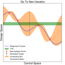
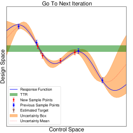
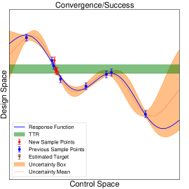
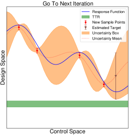
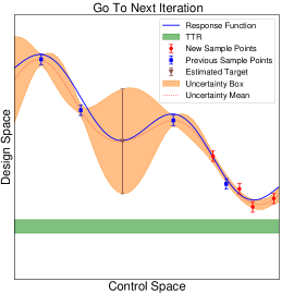
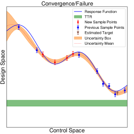
Figure 1: Schematic illustration of the TAD algorithm. The panels display an idealized problem in which the control space is collapsed onto the $x$-axis and the design space is collapsed onto the $y$-axis. The algorithm samples the control space to discover the shape of the response surface while searching the space for the target design. The top panels illustrate the case where a control setting exists such that the target design exists, within tolerance. The bottom panels illustrate the case where no such design is to be found.

The TAD algorithm in effect defines the TTR— a rectangular parallelepiped centered on the target design $f_{T}$—and iterates, at each iteration maximizing $\mathcal{L}_{TAD}(x,\bm{x}_{1},\bm{g}_{1},\bm{x}_{2})$ with respect to new sample points $\bm{x}_{2}$ and a target point $x$, either until the predicted mean design and its uncertainty (as computed by using Equations 12 and 15) fit inside the TTR or until it is possible to conclude that no point satisfying this condition exists in the control space $X$.

The process is illustrated in idealized form in Figure Fig. 1, in which the control space $X$ and the design space $Y$ are collapsed to one dimension and displayed as the $x$-axis and $y$-axis of the figure illustrations, respectively. The solid blue curve shows the experimental response, while the TTR is illustrated by the horizontal green band stretching across each plot. New ($\bm{x}_{2},\bm{g}_{2}$) noisy sample points are shown as red circle markers, while old ($\bm{x}_{1},\bm{g}_{1}$) sample points are shown as blue square markers. The Gaussian process model mean is shown by the dotted line, while the 1-$\sigma$ variance model uncertainty is shown by the shaded area. At each stage the control point closest in predictive probability to the target, together with its uncertainty, is shown by the brown triangle marker and error bar.

The top panels illustrate the case where a solution exists in the search space and show how the algorithm is intended to preferentially shrink the uncertainty in the response surface in regions where the predictive probability of the target is highest until the solution is located. The lower panels illustrate the other possible case: a solution does not exist, possibly because the TTR has been specified too stringently for some design feature. In this case, TAD shrinks the uncertainty in the function to the point where it can conclude (in a manner more systematic than merely glancing at a graphical illustration!) that no such solution exists. As this discussion illustrates, optimization of the TAD acquisition function $\mathcal{L}_{TAD}()$ in the algorithm sketched above (and to be described in detail below) provides a tool for balancing the competing objectives of exploration and exploitation, the classic tension between discovering the global shape of the response function and discovering the optimal response point.

3.1 Tolerances and Stopping Rules

Clearly the question of convergence has to do with whether the uncertainty associated with the estimated best target control point fits inside the TTR. For making this comparison, let us define the uncertainty box (UB) of the unknown function in a manner similar to the TTR, which is to say simply a rectangular parallelepiped at each control point $x\in X$ centered on the current GP model mean vector at $x$, $p^{{(f(x)|1)}}$, with sides along each coordinate axis in $Y$ of length equal to twice the corresponding root variance (diagonal element of $Q^{(f(x)|1+2)}$). The reason for defining the UB this way, instead of by an appeal to the principal ellipsoids of the covariance $Q^{(f(x)|1+2)}$), is for ease of comparison with the TTR and because no real benefit accrues from the algebraic complexity that arises from a too-principled geometric approach here.

Initially the surrogate function is assumed known vaguely, and the (prior) UB at each point is wide enough to contain the TTR. At each iteration TAD chooses sample points to “squeeze” the UB selectively in regions of the control space where target design seems most likely, according to the current model. This variance reduction may improve the chances of locating the target in the region of interest, in which case more attention is focused on this region and more sample points are invoked to exploit its solution-bearing potential. Alternatively, the variance reduction may make the target less likely in this region, or even put the UBs of points in this region definitively outside of the TTR, in which case sample points are directed to more promising regions.

If a region is discovered to hold a point where a UB fits entirely within the TTR, the algorithm declares convergence and a successful solution. This condition is called “convergence/success.”

Alternatively, the algorithm can signal that it is giving up on the search by transitioning from the “Hopeful Path” to the “Hopeless Path” of optimization, a transition that is clearly detectable in a decline in expected information $\mathcal{I}()$ to very small values. By thresholding on $\mathcal{I}()$, TAD declares convergence with no solution. This condition is called “convergence/failure.”

These considerations are admittedly heuristic. We do not have a proof that $\mathcal{I}()$ must eventually decline and remain below some threshold, nor have we derived the rate at which decline should occur on average. Such results might be obtainable through results on average and/or optimal learning curves describing the rate of decline of GP generalization error with training data size [36, 23, 39]. Here we confine ourselves to noting that in our numerical experiments such as the ones described in $\S$4 we observe $\mathcal{I}()$ to decline noisily but steadily enough to provide a useful gauge of solution failure.

Note the considerable benefit that has followed from the information-theory approach: while “convergence/success” is a local criterion, “convergence/failure” is a global statement about the absence of a solution in $X$ satisfying the required tolerances. Ironically, it is much harder to fail properly than it is to succeed! A naive approach to establishing a “convergence/failure” criterion—say, an explicit search of $X$, partitioned a priori into search volumes—could be expensive if the dimension $D$ of $X$ is even moderately large. As matters stand, the TAD acquisition function $\mathcal{L}()$ provides a built-in efficient strategy to search $X$, and the expected information $\mathcal{I}()$ furnishes a gauge of when that search transitions from hopeful to hopeless, providing exactly the required “convergence/failure” criterion.

3.2 Model Validation

Algorithm 1 Targeted Adaptive Design

1:TTR $\eta_{\mathrm{TTR}}$ with component intervals $\eta_{i}\leftarrow\left[f_{Ti}-\tau_{i},f_{Ti}+\tau_{i}\right]$, $i=1,\ldots,E$, where $\tau_{i}$ is the $i$-th component of the tolerance vector $\tau$, and $f_{Ti}$ is the $i$th component of the target vector $f_{T}$

2:$\mathcal{I}_{0}$, expected information threshold, and $N_{\mathcal{I}}$ number of consecutive iterations in which $\mathcal{I}<\mathcal{I}_{0}$ required to declare convergence/failure

3:$\bm{x}_{1}$, a set of initial design points of size $N_{1}$, and the corresponding samples $\bm{g}_{1}$

4:$x$, a target control point initialization

5:$\bm{x}_{2}\leftarrow\left\{x_{2,l}\sim\mathcal{N}\left[x,\sigma^{2}\bm{I}_{D}\right]:l=1,\ldots,N_{2}\right\}$, initial cluster of proposed sample settings

6:$Converged\leftarrow\textbf{False}$, $Check\_Model\leftarrow\textbf{False}$, $Perturb\leftarrow\textbf{True}$

7:$iter\leftarrow 0$, $n\_check\leftarrow 0$, $P\leftarrow 2$, $n_{\mathcal{I}}\leftarrow 0$

8:while $\textbf{not}\;Converged$ do

9:     if $\textbf{not}\;Check\_Model$ then

10:         $iter\leftarrow iter+1$

11:         Solve the GP optimization problem Eq. 26 for hyperparameters $\mu$, $\theta$.

12:     end if

13:     $x^{(0)}\leftarrow x$, $\bm{x}_{2}^{(0)}\leftarrow\bm{x}_{2}$

14:     $x,\bm{x}_{2}\leftarrow\mathrm{TAD\_OPT}\left(x^{(0)},\bm{x}_{2}^{(0)},Perturb\right)$ $\triangleright$ See Algorithm 2

15:     Compute $Q$ using Eq. 27

16:     if $Q>0.01$ then

17:         $Check\_Model\leftarrow\textbf{False}$, $n\_check\leftarrow 0$

18:         Call Procedure Check_Convergence $\triangleright$ See Algorithm 3

19:         Acquire data $\bm{g}_{2}$ at $\bm{x}_{2}$ and $g$ at $x$

20:         $\bm{x}_{1}\leftarrow\bm{x}_{1}\cup\bm{x}_{2}\cup x$, $\bm{g}_{1}\leftarrow\bm{g}_{1}\cup\bm{g}_{2}\cup g$; $Perturb\leftarrow\textbf{True}$

21:     else

22:         $n\_check\leftarrow n\_check+1$

23:         if $n\_check==2$ then $\triangleright$ Model validation failure

24:              $P\leftarrow P+1$ $\triangleright$ Increase number of Kronecker products

25:              Acquire data $\bm{g}_{2}$ at $\bm{x}_{2}$

26:$\triangleright$ Guard against failing validation due to data inadequacy

27:              $\bm{x}_{1}\leftarrow\bm{x}_{1}\cup\bm{x}_{2}$, $\bm{g}_{1}\leftarrow\bm{g}_{1}\cup\bm{g}_{2}$

28:              $\bm{x}_{2}\leftarrow\bm{x}_{2}^{(0)}$, $x\leftarrow x^{(0)}$, $Perturb\leftarrow\textbf{False}$ $\triangleright$ Restart from previous state

29:              $n\_check\leftarrow 0$, $Check\_Model\leftarrow\textbf{False}$

30:         else$\triangleright$ Model validation alert, but not yet alarm

31:              Acquire data $\bm{g}_{2}$ at $\bm{x}_{2}$ and $g$ at $x$

32:              $\bm{x}_{1}\leftarrow\bm{x}_{1}\cup\bm{x}_{2}\cup x$,$\bm{g}_{1}\leftarrow\bm{g}_{1}\cup\bm{g}_{2}\cup g$

33:              $Perturb\leftarrow\textbf{True}$, $Check\_Model\leftarrow\textbf{True}$

34:         end if

35:     end if

36:end while

Algorithm 2 TAD Optimization Function

1:function TAD_OPT($x^{(0)}$, $\bm{x}_{2}^{(0)}$, Perturb)

2:$\triangleright$ $x^{(0)}$ and $\bm{x}_{2}^{(0)}$ are initialization values, Perturb is Boolean

3:     if Perturb then

4:         $\bm{S}_{2}\leftarrow<(\bm{x}_{2}^{(0)}-x^{(0)})(\bm{x}_{2}^{(0)}-x^{(0)})^{T}>$

5:         Initialize $x\leftarrow x_{\epsilon}\sim\mathcal{N}\left[x^{(0)},\epsilon\right]$;

6:         Initialize $\bm{x}_{2}$: $x_{2,1}\leftarrow x_{\epsilon}\sim\mathcal{N}\left[x^{(0)},\epsilon\right]$; $x_{2,l}\leftarrow z_{2}\sim\mathcal{N}\left[x_{0},\bm{S}_{2}\right]$, $l=2,\ldots,N_{2}$

7:$\triangleright$ $\epsilon$ is a “small” perturbing covariance

8:     else

9:         Initialize $x\leftarrow x^{(0)}$

10:         Initialize $\bm{x}_{2}\leftarrow\bm{x}_{2}^{(0)}$

11:     end if

12:     Solve the TAD optimization problem Eq. 18 for $x$ and $\bm{x}_{2}$.

13:     return $x$, $\bm{x}_{2}$

14:end function

Algorithm 3 TAD Convergence Testing Procedure

1:procedure Check_Convergence

2:     Calculate UB $u$:

3:$u_{i}\leftarrow\left\{p^{(f(x)|1)}-\left[\left(Q^{(f(x)|1+2)}\right)_{ii}\right]^{1/2},p^{(f(x)|1)}+\left[\left(Q^{(f(x)|1+2)}\right)_{ii}\right]^{1/2}\right\}$, $i=1,\ldots,E$

4:     $Convergence/Success\leftarrow\forall(i\in\mathbb{N};i>0;i\leq E)\,u_{i}\subset\eta_{i}$

5:     Calculate $\mathcal{I}(x,\bm{x}_{1},\bm{g}_{1},\bm{x}_{2})$ according to Equation Eq. 22

6:     if $\textbf{not}\;Convergence/Success\;\textbf{and}\;\mathcal{I}(x,\bm{x}_{1},\bm{g}_{1},\bm{x}_{2})<\mathcal{I}_{0}$ then

7:         $n_{\mathcal{I}}\leftarrow n_{\mathcal{I}}+1$

8:     end if

9:     $Convergence/Failure\leftarrow n_{\mathcal{I}}>N_{\mathcal{I}}$

10:     $Converged\leftarrow Convergence/Success\;\textbf{or}\;Convergence/Failure$

11:end procedure

Our experience with TAD has led us to be cautious about trusting conclusions drawn from an unvalidated GP model. Indeed, more than once our intuition about the expected behavior of the algorithm, which we based on what appeared to be sound mathematics, foundered on problems due to model inadequacy. As we noted in Section 2.5, one should expect a progressive loss of model adequacy as successive iterations of the algorithm introduce more sample data and better knowledge of the structure of the response function. We have therefore built into the algorithm an anticipation of loss of model adequacy with iteration number, as well as a mechanism for dynamic increase of model complexity where required.

Model complexity could be increased in a few different ways, by choosing different types of basis kernel functions, for example. In this work we choose the simplest option, which is to parameterize model complexity by the number $P$ of Kronecker components in Equation Eq. 24. When we need to complexify the model, we add a Kronecker component, thus increasing $P$ by 1.

We monitor model adequacy using the quantity $Q$ defined in Equation Eq. 27. We set a smallness threshold for this quantity, 0.01, for example, and complexify the model if $Q$ falls below this value. In order to guard against unnecessary complexification, each time a validation test at the end of a TAD optimization produces a value of $Q$ indicating model inadequacy, we restart the optimization from a different random initialization of the $\bm{x}_{2}$ sample point locations. If the reinitialized optimization still indicates model inadequacy, then model complexity is increased. Otherwise the event is considered a false alarm.

In addition, prior to each such restart, we acquire the data $\bm{g}_{2}$ at the $\bm{x}_{2}$ sample point locations from the TAD optimization solution that “failed” validation. The reason is the observation from Section 2.5 that in early iterations, when only a few $(\bm{x}_{1},\bm{g}_{1})$ samples covering small regions of $X$ are available, the GP model parameter optimization usually produces surrogate models that are not representative of the behavior of the experimental response function over the whole of $X$. In such cases, it is perfectly possible for a $Q$ value to flunk a validation test, not because of lack of model complexity, but because of data inadequacy.

3.3 Outline of the TAD Algorithm

We now discursively outline the TAD algorithm, so that we can discuss various elements below. The formal definition of TAD is given as Algorithm 1.

We select an initial design $\bm{x}_{1}$ of size $N_{1}$ and acquire the corresponding points $\bm{g}_{1}$. We have found that if one wishes to allow plenty of opportunity for expected improvement at the outset of the algorithm then it is useful to cluster the initial points in a region of $X$. However, the initial design is in principle arbitrary, and may span $X$, or be chosen as a Latin Hypercube, for example.

We fix $N_{2}$, the number of $(\bm{x}_{2},\bm{g}_{2})$ samples to be acquired at each new iteration (in principle $N_{2}$ could change adaptively with iteration number to create a more flexible algorithm in the same family).

At the outset (iteration $I=0$), the TTR is constructed, and a convergence/failure threshold $\mathcal{I}_{0}$ for expected information is set. Since $\mathcal{I}$ can fluctuate during the optimization and hence can rise back up above $\mathcal{I}_{0}$ after first crossing the threshold, we also set a parameter $N_{\mathcal{I}}$, representing the number of consecutive iterations during which it must remain the case that $\mathcal{I}<\mathcal{I}_{0}$ in order to declare convergence/failure. The initial model complexity $P$ is chosen. The target location $x$ is initialized randomly. The sample point locations $\bm{x}_{2}$ are selected randomly in some small region near $x$ using a multivariate normal with mean $x$ and a unit-proportional covariance (for simplicity). The corresponding sample values $\bm{g}_{2}$ are acquired. The initial $\bm{x}_{1}$-sample set is chosen to be some modest-sized design.

At iteration $I$ the algorithm performs the following steps:

1. Optimize the GP log-likelihood $\mathcal{L}_{GP}(\mu,\theta)$ with respect to the GP model hyperparameters $\mu$ and $\theta$ (Equation Eq. 26), verifying that the quadratic form $S$ in Equation Eq. 28 takes plausible values, as described in §subsec:validation.

2. Compute the empirical covariance $\bm{X}_{2}\equiv<(\bm{x}_{2}-x)(\bm{x}_{2}-x)^{T}>$ of the previous $\bm{x}_{2}$-sample locations about the target location (see note below), and sample a set of $N_{2}-1$ initialization values $\bm{x}_{2,0}\sim\mathcal{N}\left\{x,\bm{X}_{2}\right\}$. The remaining initialization value is chosen at a small perturbation of $x$, the perturbation size selected to be large enough not to induce numerical instability in computations of covariances with nearly redundant rows.

3. Optimize the TAD acquisition function $\mathcal{L}_{TAD}(x,\bm{x}_{1},\bm{g}_{1},\bm{x}_{2})$ with respect to the sample locations $\bm{x}_{2}$ and target location $x$, initializing the optimization target location $x$ from the value of $x$ found at the previous iteration and initializing the $\bm{x}_{2}$ by $\bm{x}_{2}=\bm{x}_{2,0}$ (Equation Eq. 18).

4. Perform model validation, by computing the quadratic form $Q$ of Equation Eq. 27 and checking whether it takes plausible values, as described in Section 3.2. If it does not, restart the previous step; and if the failure persists, complexify the model by adding a Kronecker component. Otherwise, proceed.

5. Test for convergence/success condition: construct the UB at $x$, and test whether all of its components fit inside the TTR. If so, declare convergence/success; report the solution control setting $x$, the corresponding design $p^{(f(x)|1)}$, and predictive covariance $Q^{(f(x)|1+2)}$; and stop. Otherwise continue.

6. Test for convergence/failure condition: compute $\mathcal{I}(x,\bm{x}_{1},\bm{g}_{1},\bm{x}_{2})$ using Equation Eq. 23, and test whether $\mathcal{I}(x,\bm{x}_{1},\bm{g}_{1},\bm{x}_{2})<\mathcal{I}_{0}$. If so and if this has occurred for more than $N_{\mathcal{I}}$ consecutive iterations, declare convergence/failure, and stop; otherwise continue.

7. Acquire sample of data $\bm{g}_{2}$ at newly determined sample points $\bm{x}_{2}$, and target data $g$ from latest estimated target point $x$.

8. Proceed to iteration $I+1$.

At Item 2 we have found empirically that it is in general better to compute the scatter of the $\bm{x}_{2}$ points about the target point $x$ than about the mean $\bm{x}_{2}$ point. The reason is that in an exploitation phase, there is not much difference, but in exploration the $\bm{x}_{2}$ points often need to be initialized with greater variance in order to sense the optimal direction of $\mathcal{L}_{TAD}()$. The target point usually “leads” the cloud of $\bm{x}_{2}$ points during exploration, which elongates the principal axes of the covariance $\bm{X}_{2}$ that extend in the direction from the $\bm{x}_{2}$ points to the target point. We have found that this initialization has a beneficial impact on the TAD optimization problem Eq. 18.

At Item 3 it is important to initialize the target point $x$ at or very near the solution from the previous iteration. Doing so allows the acquisition function to increase monotonically while exploiting a possible solution. It is also useful to initialize the $\bm{x}_{2}$ sample locations near $x$ and at remixed values of $\bm{x}_{2}$, in order to begin adding information to what is already available from the previous iteration.

3.4 Implementation

Our implementation of the TAD algorithm is hosted at a GitHub repository [22] and implemented in Python. The GP portion of the implementation is built on top of GPyTorch [26, 12]. The reason for this choice is that the GPyTorch package implements fast kernel methods such as the SKI inducing point method described in [40], while exploiting the GPU acceleration facilities built into the PyTorch deep learning framework. These features hold great promise for large GP kernel matrix performance and appear to have broken through the “curse of dimensionality” problem of GP modeling and prediction, allowing computation with covariance matrices so large that they must be computed on the fly, because they cannot be affordably stored [12].

These are choices that we have made with an eye to the future, in view of the potential for large-scale optimization problems that may arise in the exploration of advanced manufacturing control spaces. For example, Paulson et al. [24] describe exploration of flame spray pyrolysis experimental controls with $D=6$, in which the design objective is to control features of the particle formation size spectrum—three moments of the spectrum in the case described, although there is no reason a more complex description might not be required. Even granting that TAD can do much better than a naive sampler, with a fixed grid on each axis, one can easily see how the classic computational costs of GP modeling, which grow as $N^{3}$ (where $N$ is the dimensionality of the covariances in question), might make such modeling unaffordable in the absence of the new methods.

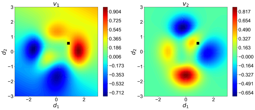
Figure 2: Test function for numerical experiments. The black square is the location of the target value for the “convergence/success” test.

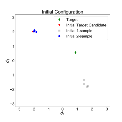
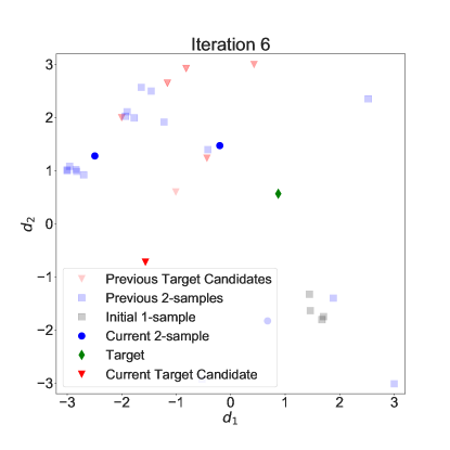
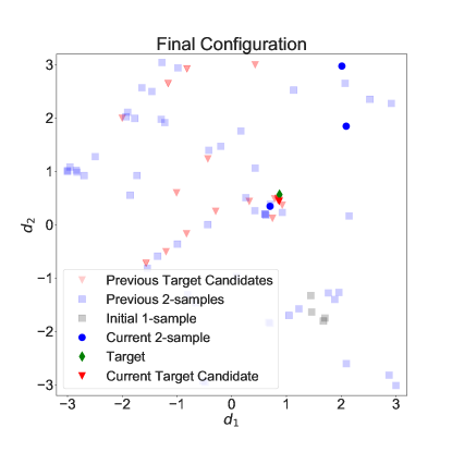
Figure 3: Evolution of TAD “2” samples and solution.

4 Numerical Results

4.1 Twin-peak problem

The TAD class has no existing problems. For testing purposes we use a problem taken from [1] with a $D=2$-dimensional control space and an $E=2$-dimensional design space. The two-dimensional vector function $(v_{1},v_{2})$ has the form

(29) $$v_{1}(d_{1},d_{2})=3(1-d_{1})^{2}e^{-d_{1}^{2}-(d_{2}+1)^{2}}-10(d_{1}/5-d_{1}^{3}-d_{2}^{5})e^{-d_{1}^{2}-d_{2}^{2}}\\ -3e^{-(d_{1}+2)^{2}-d_{2}^{2}}+0.5(2d_{1}+d_{2});$$

(30) $$v_{2}(d_{1},d_{2})=3(1+d_{2})^{2}e^{-d_{2}^{2}-(d_{1}+1)^{2}}-10(-d_{2}/5+d_{2}^{3}+d_{1}^{5})e^{-d_{1}^{2}-d_{2}^{2}}\\ -3e^{-(2-d_{2})^{2}-d_{1}^{2}}+0.5(2d_{1}+d_{2}),$$

where $(d_{1},d_{2})\in[-3,3]^{2}$. The behavior of the function is displayed in Figure Fig. 2.

4.1.1 Convergence/Success

We tested the convergence/success path of the algorithm by searching for the target $f_{T}=[0.3380,3502]$ with tolerance $\tau=0.01$. This value occurs in the domain at $[d_{1},d_{2}]=[0.8731,0.5664]$, shown by the black square in Figure Fig. 2. We adopted convergence/failure criteria of $\mathcal{I}_{0}=10^{-3}$, $N_{\mathcal{I}}=50$. The initial design was a set of $N_{1}=4$ points in the vicinity of $[d_{1},d_{2}]=[1.5,-1.5]$. We used $N_{2}=3$ and started the test at $x=[-2.0,2.0]$.

Convergence occurred in 18 iterations, requiring a total of 70 sample points. The initial and final sample point configurations and two intermediate snapshots are displayed in Fig. 3. In each case, previously acquired samples are displayed with partial transparency, while the current $\bm{x}_{2}$ samples and target value are displayed solidly, as is the true target solution. These figures clearly show that the algorithm is engaging in some balance between feeling out the response function and hunting for the target value.

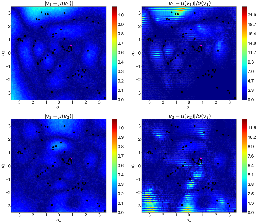
Figure 4: Pointwise residuals. Left column: Absolute residuals between predictive mean and target function. Right column: Residuals normalized to root predictive variance.

The pointwise residuals of the GP surrogate at the final iteration are displayed in Fig. 4. The left panels show unnormalized residuals, whose magnitudes are not as straightforward to interpret as those of the residuals normalized to root predictive variance, shown in the right panels. These are expected to be of order unity in regions where the GP surrogate furnishes a reasonable model of the experimental response. From the figure, it is clear that this is, unsurprisingly, true only in the vicinity of the sample points.

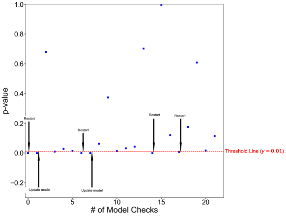
Figure 5: Model validation, convergence/success case.

The model validation and dynamic model complexification mechanism is visualized in Fig. 5. The figure shows the $P$-value threshold as a horizontal dashed line and the $P$-values ascertained at each iteration as square markers. The downward-pointing arrows show model validation failure alerts, where restarts occur. The subsequent upward-pointing arrows show confirmations of validation failures, where the GP model is updated by increasing the number of Kronecker components. The plot shows that after an initial couple of rounds of model validation failures, the surrogate model gained enough complexity to represent the portion of the response surface required to exploit the solution.

The run of expected information gain and of the log-Gaussian term is displayed in Fig. 6. The initial drop in expected information is associated with the refinement of the initially crude model. In this study the algorithm found an exploitation mode very early. As can be seen from Fig. 3, by iteration 7 the target point $x$ was already in the neighborhood of the solution; and in the remaining iterations the drop in log-Gaussian represents the effort to obtain convergence by squeezing the UB into the TTR.

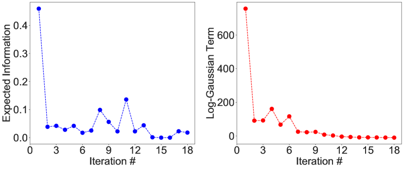
Figure 6: Expected information gain and log-Gaussian term vs number of iterations, convergence/success case.

4.1.2 Convergence/Failure

We tested the convergence/failure path of the algorithm by searching for the target $f_{T}=[-1,-1]$, which does not occur in the domain, with tolerance $\tau=0.01$. We adopted convergence/failure criteria of $\mathcal{I}_{0}=10^{-3}$, $N_{\mathcal{I}}=50$. The initial design was the same set of $N_{1}=4$ points as for the convergence/success test. We used $N_{2}=3$ and started the test at $x=[2.0,2.0]$.

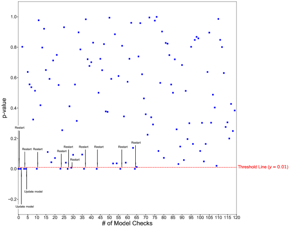
Figure 7: Model validation, convergence/failure case.

The algorithm declared convergence/failure after 111 iterations, requiring 442 sample points in all. Fig. 7 shows the model validation and dynamic model complexification mechanism. Once again we see an initial period of model inadequacy. There follows a cycle of exploration punctuated by occasional model validation alerts, all but two of which are false positives.

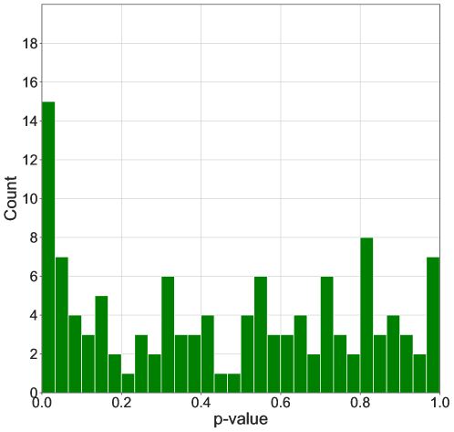
Figure 8: Histogram of $P$-values from Fig. 7.

The distribution of $P$-values appearing in Fig. 7 is displayed in Fig. 8. Other than the spike of small $P$-values caused by validation failures that trigger model complexifications, the histogram appears reasonably uniform, as it should.

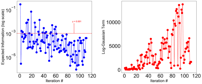
Figure 9: Expected information gain and log-Gaussian term, convergence/failure case.

Fig. 9 shows the run of expected information gain and of the log-Gaussian term. Here we see a logarithmic decline in expected information gain as the uncertainty is squeezed out of the surrogate response. Monitoring expected information gain for this kind of drop results in an effective convergence/failure criterion.

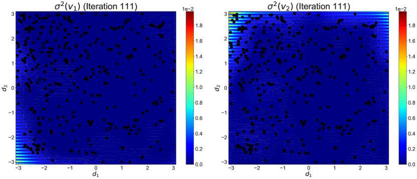
Figure 10: Variance at convergence/failure.

Fig. 10 displays the surrogate model variance at the final iteration when convergence/failure is declared. At this stage the algorithm has sampled the space fairly uniformly and has generated a relatively smooth model of the variance for both components of the vector field.

Figure 11: Pointwise residuals. Left column: Absolute residuals between predictive mean and target function. Right column: Residuals normalized to root predictive variance.

Fig. 11 displays the residuals between the surrogate model and the target function. The right-hand panels display the normalized residual, expected to be of order unity, with some statistical fluctuations, when the model is valid. We see that this is largely the case, with some residual model inadequacy near the domain edge and in some patches of less-dense sampling.

4.2 DTLZ4 problem

The DTLZ problem test suite is constituted of benchmark problems for multiobjective optimization. These problems were developed by Deb, Thiele, Laumanns and Zitzler [9] and are particularly for scalable multiobjective optimization as the number of variables, as well as the number of objective functions, can be tuned. In this work, we use the dtlz4 problem

$$f_{1}(x) = (1+g(x_{M}))\cos(x_{1}^{\alpha}\pi/2)\cdots\cos(x_{M-2}^{\alpha}\pi/2)\cos(x_{M-1}^{\alpha}\pi/2)$$

$$f_{2}(x) = (1+g(x_{M}))\cos(x_{1}^{\alpha}\pi/2)\cdots\cos(x_{M-2}^{\alpha}\pi/2)\sin(x_{M-1}^{\alpha}\pi/2)$$

$$\vdots$$

$$f_{M}(x) = (1+g(x_{M}))\sin(x_{1}^{\alpha}\pi/2)$$

$$\text{with }g(x_{M}) = \sum_{x_{i}\in x_{M}}(x_{i}-0.5)^{2},\;\alpha=100\;\text{and}\;\;0\leq x_{i}\leq 1\;\;\text{for }i=1,2,\cdots,n.$$

The last $k=n-M+1$ variables are represented in $x_{M}$. See [4] for more details.

4.2.1 Convergence/Success

We set the number of control variables to $n=4$ control variables and the number of tasks to $M=3$. The target value is $f_{T}=[1.0607,0.0109,0.0040]$. We set the noise value at $0.0001$ and the tolerance at $1\%$. TAD found a design value of $f_{TAD}=[1.0474e,0.025,0.00025]$ after 6 iterations with 4 model updates i.e. 5 total Kronecker products needed. The behavior of the expected information gain and the log-Gaussian term is displayed in Figure 12.

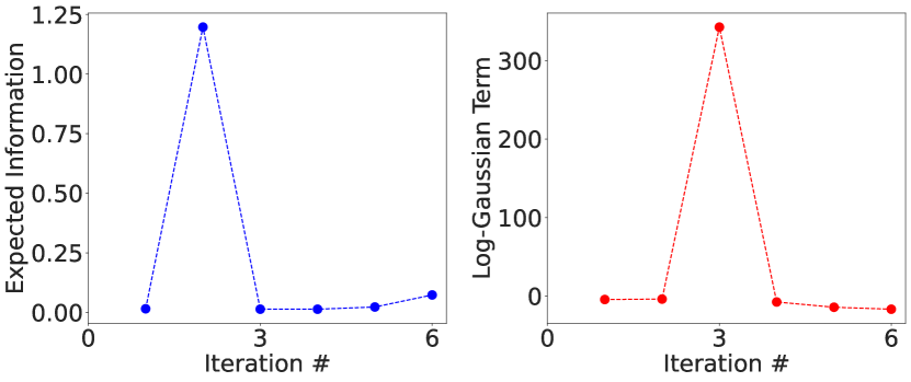
Figure 12: Expected info and log gaussian term for the dtlz4 problem, convergence/success.

4.2.2 Convergence/Failure

We set the number of control variables to $n=4$ control variables and the number of tasks to $M=3$. The target value is $f_{T}=[2.,2.,2.]$ which is not feasible. As for the convergence/success case, the noise value is $0.0001$ and the tolerance at $1\%$. Figure 13 displays behavior of the expected information gain and the log-Gaussian term. TAD needed three Kronecker products and failed in $57$ iterations as.

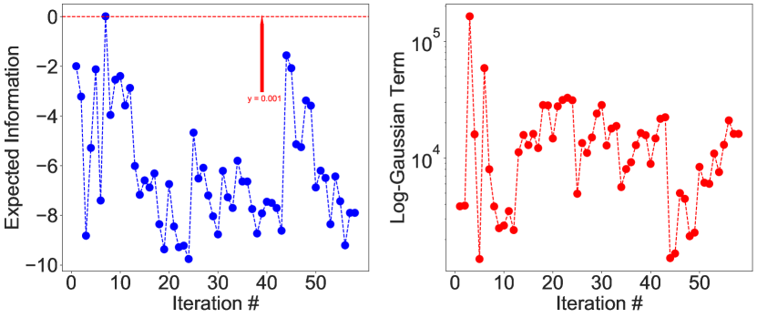
Figure 13: Expected information gain and log-Gaussian term for the dtlz4 problem in log scale, convergence/failure case.

5 Discussion

We have given some theory and some empirical experience to justify the design of TAD, a new algorithm for data-driven sequential discovery of optimal control settings for advanced manufacturing equipment. The algorithm is designed to track uncertainty in multiple design feature dimensions, so as to be capable of satisfying simultaneous specified tolerance criteria within specified uncertainty.

Some noteworthy features of TAD bear comment. TAD works unproblematically with gradient-based optimization methods, unlike methods that rely on expected improvement-type criteria. EI is known not to be well suited to gradient optimization, because it tends to be multimodal with large “flat” regions of minimal change and because it is not continuously differentiable [17]. In addition, the TAD acquisition function is inexpensive to compute, unlike, for example, the knowledge gradient [42]. Such methods are thereby limited to relatively low-dimensional problems. The advanced manufacturing problem space, on the other hand, can easily lead to relatively large control and design spaces. Having a gradient method available provides some confidence that the algorithm can be scaled to larger problems.

A second reason to feel confidence in success at larger scales is the recent breakthroughs that have occurred in GP modeling with vastly more points than was possible in the past, using fast kernel approximations and GPU acceleration [40, 12]. Given that high-dimensional control and design spaces might require many iterations and numerous samples to reach convergence and that the associated GP and TAD optimization problems can therefore technically require many potentially expensive linear solves, the availability of fast methods seems likely to be important.

The importance of validation, principally by means of LOO validation, has been emphasized by, for example, [17, 3]. It is worth driving home again. A Gaussian process surrogate whose validity is not assiduously monitored has every chance of making poor predictions, and no algorithm founded on such a model is secure no matter how sound its mathematical foundation. Oddly we have not found any references in the literature to the seemingly obvious idea of using the $\chi^{2}$ distribution with the predictive distribution of a batch of samples, in the manner that we described in Section 2.5. This is a straightforward validation test that offers sensitivity gains over straight LOO and that comes practically for free since the linear solve of a GP prediction is an inner product away from the quadratic form that yields $\chi^{2}$.

In real-world manufacturing applications the highly simplified model represented by the mapping $X\rightarrow Y$ from control space to design space can be clouded. For example, a product’s desired design properties might require so-called ex situ measurements at facilities external to the manufacturing facilities [41], and this requirement can introduce long time latencies in the measurement of the experimental response function that vitiate the practical application of a direct TAD-based methodology. In such cases one can still envision a place for the TAD algorithm in the design workflow. For example, in additive manufacturing, it is pointed out in [30] that complex but discernible relationships can exist between process (i.e., promptly measured) manufacture parameters and final structure, property, and performance parameters of a product. Even when those parameters must be validated externally, a TAD workflow targeted at a known-good region of a process-parameter space from a high-dimensional control space could cut down considerably on the number of test pieces that must be sent to the external test facility for validation.

Appendix A Gaussian Prediction Update Formula

Suppose a vector-valued random variable of dimension $1+N_{1}+N_{2}$, written in partitioned form $[f,\bm{g}_{1},\bm{g}_{2}]^{T}$, has a multivariate normal distribution,

(31) $$\begin{bmatrix}f\\ \bm{g}_{1}\\ \bm{g}_{2}\end{bmatrix}\sim\mathcal{N}\left\{\begin{bmatrix}m\\ \bm{m}_{1}\\ \bm{m}_{2}\end{bmatrix},\begin{bmatrix}C_{ff}&\bm{C}_{f1}&\bm{C}_{f2}\\ \bm{C}_{1f}&\bm{C}_{11}&\bm{C}_{12}\\ \bm{C}_{2f}&\bm{C}_{21}&\bm{C}_{22}\end{bmatrix}\right\},$$

where $f$ and $m$ are 1-dimensional, $\bm{g}_{1}$ and $\bm{m}_{1}$ are $N_{1}$-dimensional, $\bm{g}_{2}$ and $\bm{m}_{2}$ are $N_{2}$-dimensional, and the various covariance matrix partitions have the obvious necessary dimensions.

The usual normal theory conditioning formulae allow us to write the distributions for $\bm{g}_{2}|\bm{g}_{1}$, $f|\bm{g}_{1}$ and $f|(\bm{g}_{1},\bm{g}_{2})$:

(32) $$\bm{g}_{2}|\bm{g}_{1} \sim\mathcal{N}\left(\bm{p}^{(2|1)},\bm{Q}^{(2|1)}\right)$$

(33) $$\bm{p}^{(2|1)} =\bm{m}_{2}+\bm{C}_{21}\bm{C}_{11}^{-1}(\bm{g}_{1}-\bm{m}_{1})$$

(34) $$\bm{Q}^{(2|1)} =\bm{C}_{22}-\bm{C}_{21}\bm{C}_{11}^{-1}\bm{C}_{12}.$$

(35) $$f|\bm{g}_{1} \sim\mathcal{N}(p^{(f|1)},Q^{(f|1)})$$

(36) $$p^{(f|1)} =m+\bm{C}_{f1}\bm{C}_{11}^{-1}(\bm{g}_{1}-\bm{m}_{1})$$

(37) $$Q^{(f|1)} =C_{ff}-\bm{C}_{f1}\bm{C}_{11}^{-1}\bm{C}_{1f}.,$$

and

(38) $$f|\bm{g}_{1},\bm{g}_{2} \sim\mathcal{N}\left\{p^{(f|1+2)},Q^{(f|1+2)}\right\}$$

(39) $$p^{(f|1+2)} =m+\begin{bmatrix}\bm{C}_{f1}&\bm{C}_{f2}\end{bmatrix}\begin{bmatrix}\bm{C}_{11}&\bm{C}_{12}\\ \bm{C}_{21}&\bm{C}_{22}\end{bmatrix}^{-1}\begin{bmatrix}\bm{g}_{1}-\bm{m}_{1}\\ \bm{g}_{2}-\bm{m}_{2}\end{bmatrix}$$

(40) $$Q^{(f|1+2)} =C_{ff}-\begin{bmatrix}\bm{C}_{f1}&\bm{C}_{f2}\end{bmatrix}\begin{bmatrix}\bm{C}_{11}&\bm{C}_{12}\\ \bm{C}_{21}&\bm{C}_{22}\end{bmatrix}^{-1}\begin{bmatrix}\bm{C}_{1f}\\ \bm{C}_{2f}\end{bmatrix}.$$

In the main text, the interpretation of $\bm{g}_{1}$ is “data in the can,” while that of $\bm{g}_{2}$ is “data that could be acquired at the next iteration,” and $f$ is a latent value to be predicted. It is therefore useful to re-express the predictive distribution $f|(\bm{g}_{1},\bm{g}_{2})$ represented by Equations (38–40) as an update to the predictive distribution $f|\bm{g}_{1}$ represented by Equations (35–37) consequent on the updating of the data $\{\bm{g}_{1}\}\rightarrow\{\bm{g}_{1},\bm{g}_{2}\}$.

Lemma A.1 (Gaussian Prediction Update).

Update formulae from $f|\bm{g}_{1}$ to $f|(\bm{g}_{1},\bm{g}_{2})$ may be written as follows:

1. The normal means $p^{(f|1+2)}$ and $p^{(f|1)}$ are related by

   (41) $$p^{(f|1+2)}=p^{(f|1)}+\left(\bm{C}_{f2}-\bm{C}_{f1}\bm{C}_{11}^{-1}\bm{C}_{12}\right)\left(\bm{Q}^{(2|1)}\right)^{-1}\left(\bm{g}_{2}-\bm{p}^{(2|1)}\right).$$

2. The normal covariances $Q^{(f|1+2)}$ and $Q^{(f|1)}$ are related by

   (42) $$Q^{(f|1+2)}=Q^{(f|1)}-\left(\bm{C}_{f2}-\bm{C}_{f1}\bm{C}_{11}^{-1}\bm{C}_{12}\right)\left(\bm{Q}^{(2|1)}\right)^{-1}\left(\bm{C}_{2f}-\bm{C}_{21}\bm{C}_{11}^{-1}\bm{C}_{1f}\right).$$

Proof A.2.

We begin by expanding the inversion of the partitioned matrix in Equations (39) and (40) using the matrix inversion lemma (see §2.7 of [27]):

(43) $$\begin{bmatrix}C_{11}&C_{12}\\ C_{21}&C_{22}\end{bmatrix}^{-1}=\begin{bmatrix}I_{11}&I_{12}\\ I_{21}&I_{22}\end{bmatrix},$$

with

(44) $$\bm{I}_{22} \equiv\left(\bm{C}_{22}-\bm{C}_{21}\bm{C}_{11}^{-1}\bm{C}_{12}\right)^{-1}$$

(45) $$=\left(Q^{(2|1)}\right)^{-1}$$

(46) $$\bm{I}_{12} \equiv-\bm{C}_{11}^{-1}\bm{C}_{12}\bm{I}_{22}$$

(47) $$\bm{I}_{21} \equiv-\bm{I}_{22}\bm{C}_{21}\bm{C}_{11}^{-1}$$

(48) $$\bm{I}_{11} \equiv\bm{C}_{11}^{-1}+\bm{C}_{11}^{-1}\bm{C}_{12}\bm{I}_{22}\bm{C}_{21}\bm{C}_{11}^{-1}.$$

The second line notes the equality with the inverse of Equation (34).

To establish part (i), we combine Equations (39) and (43-48), obtaining an expression for the mean update:

$$p^{(f|1+2)} =m+\begin{pmatrix}\bm{C}_{f1}I_{11}+\bm{C}_{f2}I_{21}&\bm{C}_{f1}I_{12}+\bm{C}_{f2}I_{22}\end{pmatrix}\begin{pmatrix}\bm{g}_{1}-\bm{m}_{1}\\ \bm{g}_{2}-\bm{m}_{2}\end{pmatrix}$$

$$=m+\bm{C}_{f1}\left(\bm{C}_{11}^{-1}+\bm{C}_{11}^{-1}\bm{C}_{12}I_{22}\bm{C}_{21}\bm{C}_{11}^{-1}\right)\left(\bm{g}_{1}-\bm{m}_{1}\right)$$

$$+\bm{C}_{f2}\left(-I_{22}\bm{C}_{21}\bm{C}_{11}^{-1}\right)\left(\bm{g}_{1}-\bm{m}_{1}\right)$$

$$+\left[\bm{C}_{f1}\left(-\bm{C}_{11}^{-1}\bm{C}_{12}I_{22}\right)+\bm{C}_{f2}I_{22}\right]\left(\bm{g}_{2}-\bm{m}_{2}\right)$$

$$=p^{(f|1)}+\left(\bm{C}_{f1}\bm{C}_{11}^{-1}\bm{C}_{12}-\bm{C}_{f2}\right)I_{22}\bm{C}_{21}\bm{C}_{11}^{-1}\left(\bm{g}_{1}-\bm{m}_{1}\right)$$

$$-\left(\bm{C}_{f1}\bm{C}_{11}^{-1}\bm{C}_{12}-\bm{C}_{f2}\right)I_{22}\left(\bm{g}_{2}-\bm{m}_{2}\right)$$

$$=p^{(f|1)}+\left(\bm{C}_{f2}-\bm{C}_{f1}\bm{C}_{11}^{-1}\bm{C}_{12}\right)I_{22}\left[\bm{g}_{2}-\bm{m}_{2}-\bm{C}_{21}\bm{C}_{11}^{-1}\left(\bm{g}_{1}-\bm{m}_{1}\right)\right]$$

$$=p^{(f|1)}+\left(\bm{C}_{f2}-\bm{C}_{f1}\bm{C}_{11}^{-1}\bm{C}_{12}\right)\left(\bm{Q}^{(2|1)}\right)^{-1}\left(\bm{g}_{2}-p^{(2|1)}\right),$$

where in the last line we have used Equations (33) and (45).

To establish part (ii), we combine Equations (40) and (43-48) to obtain an expression for the covariance update:

$$Q^{(f|1+2)} =\bm{C}_{ff}-\bm{C}_{f1}\bm{I}_{11}\bm{C}_{1f}-\bm{C}_{f2}\bm{I}_{21}\bm{C}_{1f}-\bm{C}_{f1}\bm{I}_{12}\bm{C}_{2f}-\bm{C}_{f2}\bm{I}_{22}\bm{C}_{2f}$$

$$=\bm{C}_{ff}-\bm{C}_{f1}\bm{C}_{11}^{-1}\bm{C}_{1f}-\bm{C}_{f1}\bm{C}_{11}^{-1}\bm{C}_{12}\bm{I}_{22}\bm{C}_{21}\bm{C}_{11}^{-1}\bm{C}_{1f}$$

$$-\bm{C}_{f2}\left(-\bm{I}_{22}\bm{C}_{21}\bm{C}_{11}^{-1}\right)\bm{C}_{1f}-\bm{C}_{f1}\left(-\bm{C}_{11}^{-1}\bm{C}_{12}\bm{I}_{22}\right)\bm{C}_{2f}-\bm{C}_{f2}\bm{I}_{22}\bm{C}_{2f}$$

$$=Q^{(f|1)}-\left(\bm{C}_{f1}\bm{C}_{11}^{-1}\bm{C}_{12}-\bm{C}_{f2}\right)\bm{I}_{22}\bm{C}_{21}\bm{C}_{11}^{-1}\bm{C}_{1f}-\left(\bm{C}_{f2}-\bm{C}_{f1}\bm{C}_{11}^{-1}\bm{C}_{12}\right)\bm{I}_{22}\bm{C}_{2f}$$

$$=Q^{(f|1)}-\left(\bm{C}_{f2}-\bm{C}_{f1}\bm{C}_{11}^{-1}\bm{C}_{12}\right)\bm{I}_{22}\left(\bm{C}_{2f}-\bm{C}_{21}\bm{C}_{11}^{-1}\bm{C}_{1f}\right)$$

$$=Q^{(f|1)}-\left(\bm{C}_{f2}-\bm{C}_{f1}\bm{C}_{11}^{-1}\bm{C}_{12}\right)\left(\bm{Q}^{(2|1)}\right)^{-1}\left(\bm{C}_{2f}-\bm{C}_{21}\bm{C}_{11}^{-1}\bm{C}_{1f}\right).$$

We note—although hardly unexpected—that $p^{(f|1+2)}$ is linearly dependent on $\bm{g}_{2}$, while $Q^{(f|1+2)}$ is independent of $\bm{g}_{2}$.

Appendix B Redundant Information in The Zero-Noise Limit

The behavior of the TAD algorithm is elucidated in the text by considering the case of redundant points in the limit of zero measurement noise. In this appendix we supply the technical results to support that discussion.

Suppose that the points $\bm{x}_{1}$ and $\bm{x}_{2}$ have a subset of points $\bm{r}$ in common, so that $\bm{x}_{1}=\bm{y}_{1}\cup\bm{r}$, $\bm{x}_{2}=\bm{y}_{2}\cup\bm{r}$, $\bm{y}_{1}\cap\bm{y}_{2}=\emptyset$. We partition the submatrices of the covariance in Equation Eq. 2 accordingly:

(49) $$\Gamma\equiv\begin{bmatrix}K_{xx}&\bm{K}_{x1}&\bm{K}_{x2}\\ \bm{K}_{1x}&\bm{K}_{11}+\bm{\Sigma}_{1}&\bm{K}_{12}\\ \bm{K}_{2x}&\bm{K}_{21}&\bm{K}_{22}+\bm{\Sigma}_{2}\end{bmatrix},$$

where

(50) $$\bm{K}_{11}=\begin{bmatrix}\bm{J}_{11}&\bm{J}_{1r}\\ \bm{J}_{r1}&\bm{J}_{rr}\end{bmatrix}\quad;\quad\bm{K}_{22}=\begin{bmatrix}\bm{J}_{22}&\bm{J}_{2r}\\ \bm{J}_{r2}&\bm{J}_{rr}\end{bmatrix}\quad;\quad\bm{K}_{12}=\begin{bmatrix}\bm{J}_{12}&\bm{J}_{1r}\\ \bm{J}_{r2}&\bm{J}_{rr}\end{bmatrix},$$

(51) $$\bm{K}_{x1}=\begin{bmatrix}\bm{J}_{x1}&\bm{J}_{xr}\end{bmatrix}\quad;\quad\bm{K}_{x2}=\begin{bmatrix}\bm{J}_{x2}&\bm{J}_{xr}\end{bmatrix},$$

with $\bm{J}_{11}\equiv C(\bm{y}_{1},\bm{y}_{1})$, $\bm{J}_{1r}=\bm{J}_{r1}^{T}\equiv C(\bm{y}_{1},\bm{r})$, $\bm{J}_{rr}\equiv C(\bm{r},\bm{r})$, $\bm{J}_{22}\equiv C(\bm{y}_{2},\bm{y}_{2})$, $\bm{J}_{2r}=\bm{J}_{r2}^{T}\equiv C(\bm{y}_{r},\bm{r})$, $\bm{J}_{12}\equiv C(\bm{y}_{1},\bm{y}_{2})$, $\bm{J}_{x1}\equiv C(x,\bm{y}_{1})$, $\bm{J}_{x2}\equiv C(x,\bm{y}_{2})$, and $\bm{J}_{xr}\equiv C(x,\bm{r})$.

If we omit the redundant $\bm{r}$ points from $\bm{x}_{2}$, we obtain a nonredundant set $\bm{x}_{2}^{\prime}=\bm{y}_{2}$, in terms of which the TAD problem gives rise to the covariance $\Gamma^{\prime}$ given by

(52) $$\Gamma^{\prime}\equiv\begin{bmatrix}K_{xx}&\bm{K}_{x1}&\bm{J}_{x2}\\ \bm{K}_{1x}&\bm{K}_{11}+\bm{\Sigma}_{1}&\bm{L}_{12}\\ \bm{J}_{2x}&\bm{L}_{21}&\bm{J}_{22}+\bm{\sigma}_{2}\end{bmatrix},$$

where we have defined the block matrices $\bm{L}_{12}\equiv\bm{L}_{21}^{T}$, with

(53) $$\bm{L}_{12}\equiv\begin{bmatrix}\bm{J}_{12}\\ \bm{J}_{r2}\end{bmatrix}$$

and where $\bm{\sigma}_{2}$ is the restriction of the noise $\bm{\Sigma}_{2}$ to the nonredundant space of $\bm{y}_{2}$. We will refer to the dimensionality of the various partitioned spaces as $D_{1}^{\prime}$ for the nonredundant “$1^{\prime}$” space, $D_{2}^{\prime}$ for the nonredundant “$2^{\prime}$” space, $D_{r}$ for the redundant space, and $D_{x}$ for the prediction space. So, for example, the matrix $\bm{L}_{12}$ is $(D_{1}^{\prime}+D_{r})\times D_{2}^{\prime}$-dimensional, the matrix $\bm{J}_{2r}$ is $D_{2}^{\prime}\times D_{r}$-dimensional, $\bm{J}_{x1}$ is $D_{x}\times D_{1}^{\prime}$-dimensional, and so on.

The predictive covariance that follows from the covariance structure in Equation Eq. 49 is

(54) $$Q^{(f(x)|1+2)}=K_{xx}-\begin{bmatrix}\bm{K}_{x1}&\bm{K}_{x2}\end{bmatrix}\begin{bmatrix}\bm{K}_{11}+\bm{\Sigma}_{1}&\bm{K}_{12}\\ \bm{K}_{21}&\bm{K}_{22}+\bm{\Sigma}_{2}\end{bmatrix}^{-1}\begin{bmatrix}\bm{K}_{1x}\\ \bm{K}_{2x}\end{bmatrix},$$

while the predictive covariance that follows from the nonredundant data and the covariance in Equation Eq. 52 is

(55) $$Q^{(f(x)|1+2^{\prime})}=K_{xx}-\begin{bmatrix}\bm{K}_{x1}&\bm{J}_{x2}\end{bmatrix}\begin{bmatrix}\bm{K}_{11}+\bm{\Sigma}_{1}&\bm{J}_{12}\\ \bm{J}_{21}&\bm{J}_{22}+\bm{\sigma}_{2}\end{bmatrix}^{-1}\begin{bmatrix}\bm{K}_{1x}\\ \bm{J}_{2x}\end{bmatrix}.$$

Suppose that we set $\bm{\Sigma}_{1}=0$, and we introduce a multiplicative parameter $\epsilon$ regulating the size of $\bm{\Sigma}_{2}$, that is, $\bm{\Sigma}_{2}=\epsilon\overline{\bm{\Sigma}}_{2}$ with $\overline{\bm{\Sigma}}_{2}$ a finite noise covariance matrix, so that we can take a noise-free limit by taking the limit $\epsilon\rightarrow 0$.

As a matter of information theory, it is intuitively clear that redundant information affects predictions only up to noise and that in the noise-free limit the predictive distributions characterized by the covariances in Equations Eqs. 54 and 55 should coincide. On the other hand, as an algebraic matter it is not at all clear that the covariance in Equation Eq. 54 is even well defined, since the matrix inverse on the right-hand side of Equation Eq. 54 certainly does not exist in the limit. This is troubling because we would like to be sure of the behavior of the TAD acquisition function, Equation Eq. 11, when “2” points approach “1” points. Numerically, we are likely to encounter instabilities when this occurs. It is helpful to at least know what one ought to expect in this case if one had infinite numerical precision at one’s disposal.

The following theorem is therefore helpful.

Theorem B.1 (Noise-Free Limit).

The covariance $Q^{(f(x)|1+2)}$ has a finite limit as $\epsilon\rightarrow 0$ and, in fact, $\lim_{\epsilon\rightarrow 0}Q^{(f(x)|1+2)}=Q^{(f(x)|1+2^{\prime})}$.

Proof B.2.

Consider from the update formula, Equation 15,

(56) $$Q^{(f(x)|1+2)}=Q^{(f(x)|1)}-T,$$

where $T$ is the correction term for for the “2” information, given by

(57) $$T=\left[\bm{K}_{x2}-\bm{K}_{x1}\bm{K}_{11}^{-1}\bm{K}_{12}\right]\left(\bm{Q}^{(2|1)}\right)^{-1}\left[\bm{K}_{2x}-\bm{K}_{21}\bm{K}_{11}^{-1}\bm{K}_{1x}\right]$$

and where $\bm{Q}^{(2|1)}$ is given by Equation Eq. 10,

(58) $$\bm{Q}^{(2|1)}=\bm{K}_{22}+\bm{\Sigma}_{2}-\bm{K}_{21}\bm{K}_{11}^{-1}\bm{K}_{12}.$$

We will have a proof of the theorem if we can show that $\lim_{\epsilon\rightarrow 0}T=T^{\prime}$, where $T^{\prime}$ is the correction term for the nonredundant “$2^{\prime}$” information. $T^{\prime}$ can be written down by adapting the expression for $T$ in Equation Eq. 57 in light of a simple comparison of Equations Eqs. 49 and 52:

(59) $$T^{\prime}=\left[\bm{J}_{x2}-\bm{K}_{x1}\bm{K}_{11}^{-1}\bm{L}_{12}\right]\left(\bm{Q}^{(2^{\prime}|1)}\right)^{-1}\left[\bm{J}_{2x}-\bm{L}_{21}\bm{K}_{11}^{-1}\bm{K}_{1x}\right],$$

where

(60) $$\bm{Q}^{(2^{\prime}|1)}=\bm{J}_{22}+\bm{\sigma}_{2}-\bm{L}_{21}\bm{K}_{11}^{-1}\bm{L}_{12}.$$

The first task is to provide an asymptotic form for the term $\left(\bm{Q}^{(2|1)}\right)^{-1}$ in the limit $\epsilon\rightarrow 0$. The term in Equation Eq. 58 proportional to $\epsilon^{0}$ is $\bm{K}_{22}-\bm{K}_{21}\bm{K}_{11}^{-1}\bm{K}_{12}$. Note that according to Equations Eq. 50, the matrices $\bm{K}_{11}$ and $\bm{K}_{12}$ share their second block column. We may exploit this fact, together with the definition of the inverse matrix and the definitions in Equations Eq. 50, to evaluate $\bm{K}_{21}\bm{K}_{11}^{-1}\bm{K}_{12}$ and thereby show that

(61) $$\bm{Q}^{(2|1)}=\begin{bmatrix}\bm{z}&0\\ 0&0\end{bmatrix}+\bm{\Sigma}_{2},$$

where

(62) $$\bm{z}\equiv\bm{J}_{22}-\bm{L}_{21}\bm{K}_{11}^{-1}\bm{L}_{12}.$$

We now simplify the notation, defining the $D_{2}^{\prime}\times(D_{2}^{\prime}+D_{r})$-dimensional projection operator $\bm{P}_{2^{\prime}}$ from the redundant 2-space to the nonredundant $2^{\prime}$-space

(63) $$\bm{P}_{2^{\prime}}\equiv\begin{bmatrix}\bm{I}_{D_{2}^{\prime}}&\bm{0}\end{bmatrix}.$$

We may write

(64) $$\bm{Q}^{(2|1)}=\bm{\Sigma}_{2}+\bm{P}_{2^{\prime}}^{T}\bm{z}\bm{P}_{2^{\prime}}.$$

Equation Eq. 64 is a low-rank update to the first term on its right-hand side, so we may use the Sherman–Morrison–Woodbury lemma (see §2.7 of [27]) to obtain an expression for the inverse of $\bm{Q}^{(2|1)}$ that we require in Equation Eq. 57:

$$\left(\bm{Q}^{(2|1)}\right)^{-1} ={\bm{\Sigma}_{2}}^{-1}-{\bm{\Sigma}_{2}}^{-1}\bm{P}_{2^{\prime}}^{T}\left(\bm{z}^{-1}+\bm{P}_{2^{\prime}}{\bm{\Sigma}_{2}}^{-1}\bm{P}_{2^{\prime}}^{T}\right)^{-1}\bm{P}_{2^{\prime}}{\bm{\Sigma}_{2}}^{-1}$$

$$={\bm{\Sigma}_{2}}^{-1}-{\bm{\Sigma}_{2}}^{-1}\bm{P}_{2^{\prime}}^{T}\bigg{[}\left(\bm{P}_{2^{\prime}}{\bm{\Sigma}_{2}}^{-1}\bm{P}_{2^{\prime}}^{T}\right)^{-1}$$

(65) $$\hskip 56.9055pt-\left(\bm{P}_{2^{\prime}}{\bm{\Sigma}_{2}}^{-1}\bm{P}_{2^{\prime}}^{T}\right)^{-1}\bm{z}^{-1}\left(\bm{P}_{2^{\prime}}{\bm{\Sigma}_{2}}^{-1}\bm{P}_{2^{\prime}}^{T}\right)^{-1}+\mathcal{O}(\epsilon^{3})\bigg{]}\bm{P}_{2^{\prime}}\bm{\Sigma}_{2}^{-1},$$

where the asymptotic notation $\mathcal{O}[\epsilon^{n}]$ has the conventional meaning $x=z+\mathcal{O}[\epsilon^{n}]\Rightarrow\left|\lim_{\epsilon\rightarrow 0}(x-z)/\epsilon^{n}\right|<\infty$ and is interpreted in matrix equations as applying to all the matrix elements in the equation.

We may also compute the term $\bm{K}_{x2}-\bm{K}_{x1}\bm{K}_{11}^{-1}\bm{K}_{12}$ in Equation Eq. 57, again appealing to the common block column structure of $\bm{K}_{11}$ and $\bm{K}_{12}$ to evaluate $\bm{K}_{11}^{-1}\bm{K}_{12}$:

$$\bm{K}_{x2}-\bm{K}_{x1}\bm{K}_{11}^{-1}\bm{K}_{12} =\begin{bmatrix}\bm{J}_{x2}&\bm{J}_{xr}\end{bmatrix}-\begin{bmatrix}\bm{J}_{x1}&\bm{J}_{xr}\end{bmatrix}\bm{K}_{11}^{-1}\bm{K}_{12}$$

$$=\begin{bmatrix}\bm{q}&\bm{0}\end{bmatrix}$$

(66) $$=\bm{q}\bm{P}_{2^{\prime}},$$

where we have defined

(67) $$\bm{q}\equiv\bm{J}_{x2}-\bm{K}_{x1}\bm{K}_{11}^{-1}\bm{L}_{12}.$$

Inserting Equations Eqs. 65 and 67 into Equation Eq. 57, we find

$$T =\bm{q}\left(\bm{P}_{2^{\prime}}\bm{\Sigma}_{2}^{-1}\bm{P}_{2^{\prime}}^{T}\right)\bm{q}^{T}-\bm{q}\left(\bm{P}_{2^{\prime}}\bm{\Sigma}_{2}^{-1}\bm{P}_{2^{\prime}}^{T}\right)\left(\bm{P}_{2^{\prime}}\bm{\Sigma}_{2}^{-1}\bm{P}_{2^{\prime}}^{T}\right)^{-1}\left(\bm{P}_{2^{\prime}}\bm{\Sigma}_{2}^{-1}\bm{P}_{2^{\prime}}^{T}\right)\bm{q}^{T}$$

$$+\bm{q}\left(\bm{P}_{2^{\prime}}\bm{\Sigma}_{2}^{-1}\bm{P}_{2^{\prime}}^{T}\right)\left(\bm{P}_{2^{\prime}}\bm{\Sigma}_{2}^{-1}\bm{P}_{2^{\prime}}^{T}\right)^{-1}\bm{z}^{-1}\left(\bm{P}_{2^{\prime}}\bm{\Sigma}_{2}^{-1}\bm{P}_{2^{\prime}}^{T}\right)^{-1}\left(\bm{P}_{2^{\prime}}\bm{\Sigma}_{2}^{-1}\bm{P}_{2^{\prime}}^{T}\right)\bm{q}^{T}$$

$$+\mathcal{O}(\epsilon)$$

$$=\bm{q}\bm{z}^{-1}\bm{q}^{T}+\mathcal{O}(\epsilon)$$

(68) $$=T^{\prime}+\mathcal{O}(\epsilon).$$

It follows that $\lim_{\epsilon\rightarrow 0}T=T^{\prime}$, so the theorem is proven.

Government License

The submitted manuscript has been created by UChicago Argonne, LLC, Operator of Argonne National Laboratory (“Argonne”). Argonne, a U.S. Department of Energy Office of Science laboratory, is operated under Contract No. DE-AC02-06CH11357. The U.S. Government retains for itself, and others acting on its behalf, a paid-up nonexclusive, irrevocable worldwide license in said article to reproduce, prepare derivative works, distribute copies to the public, and perform publicly and display publicly, by or on behalf of the Government. The Department of Energy will provide public access to these results of federally sponsored research in accordance with the DOE Public Access Plan https://www.energy.gov/downloads/doe-public-access-plan.

References

- [1] A. Alfaris, Multiobjective optimization. https://ocw.mit.edu/courses/ids-338j-multidisciplinary-system-design-optimization-spring-2010/f091204b62ab5bb46825829fdedc66cd_MITESD_77S10_lec14.pdf, 2010.
- [2] M. A. Álvarez, L. Rosasco, and N. D. Lawrence, Kernels for vector-valued functions: A review, Foundations and Trends® in Machine Learning, 4 (2012), pp. 195–266, https://arxiv.org/abs/1106.6251.
- [3] D. Bingham, P. Ranjan, and W. J. Welch, Design Of Computer Experiments for Optimization, Estimation Of Function Contours, and Related Objectives, Statistics in Action: A Canadian Outlook, 109 (2014), https://arxiv.org/abs/1601.05887.
- [4] J. Blank and K. Deb, pymoo: Multi-objective optimization in python, IEEE Access, 8 (2020), pp. 89497–89509.
- [5] K. Chaloner and I. Verdinelli, Bayesian experimental design: A review, Statistical Science, 10 (1995), pp. 273–304, https://www.jstor.org/stable/pdf/2246015.pdf.
- [6] H. Cheng, J. G. Shapter, Y. Li, and G. Gao, Recent progress of advanced anode materials of lithium-ion batteries, Journal of Energy Chemistry, 57 (2021), pp. 451–468.
- [7] E. Contal, D. Buffoni, A. Robicquet, and N. Vayatis, Parallel Gaussian process optimization with upper confidence bound and pure exploration, in Joint European Conference on Machine Learning and Knowledge Discovery in Databases, Springer, 2013, pp. 225–240.
- [8] H. David and H. Nagaraja, Order Statistics, Wiley Series in Probability and Statistics, Wiley, 2004, https://books.google.com/books?id=bdhzFXg6xFkC.
- [9] K. Deb, L. Thiele, M. Laumanns, and E. Zitzler, Scalable Test Problems for Evolutionary Multiobjective Optimization, Springer London, London, 2005, pp. 105–145, https://doi.org/10.1007/1-84628-137-7_6, https://doi.org/10.1007/1-84628-137-7_6.
- [10] P. Delshad Khatibi, H. Henein, and U. Fritsching, In-Situ, Real Time Diagnostics in the Spray Forming Process, Springer International Publishing, Cham, 2017, pp. 221–263, https://doi.org/10.1007/978-3-319-52689-8_6, https://doi.org/10.1007/978-3-319-52689-8_6.
- [11] W. T. Eadie, D. Drijard, F. E. James, M. Roos, and B. Sadoulet, Statistical methods in experimental physics; 2nd ed., World Scientific, Singapore, 2006.
- [12] J. Gardner, G. Pleiss, K. Q. Weinberger, D. Bindel, and A. G. Wilson, GPyTorch: Blackbox matrix-matrix Gaussian process inference with GPU acceleration, in Advances in Neural Information Processing Systems, S. Bengio, H. Wallach, H. Larochelle, K. Grauman, N. Cesa-Bianchi, and R. Garnett, eds., vol. 31, Curran Associates, Inc., 2018, https://proceedings.neurips.cc/paper/2018/file/27e8e17134dd7083b050476733207ea1-Paper.pdf.
- [13] J. González, Z. Dai, P. Hennig, and N. Lawrence, Batch Bayesian optimization via local penalization, in Artificial intelligence and statistics, PMLR, 2016, pp. 648–657.
- [14] D. Higdon, J. Gattiker, B. Williams, and M. Rightley, Computer model calibration using high-dimensional output, Journal of the American Statistical Association, 103 (2008), pp. 570–583.
- [15] D. Huang, T. T. Allen, W. I. Notz, and R. A. Miller, Sequential kriging optimization using multiple-fidelity evaluations, Structural and Multidisciplinary Optimization, 32 (2006), pp. 369–382.
- [16] C. Jenks, H. N. Lee, J. Lewis, C. R. Kagan, P. Nealey, P. Braun, J. E. Holladay, Y. Gao, D. S. Sholl, B. A. Helms, et al., Basic research needs for transformative manufacturing, tech. report, USDOE Office of Science (SC), 2020, https://doi.org/10.2172/1618267.
- [17] D. R. Jones, M. Schonlau, and W. J. Welch, Efficient Global Optimization of Expensive Black-Box Functions, Journal of Global optimization, 13 (1998), pp. 455–492, https://doi.org/10.1023/A:1008306431147.
- [18] M. C. Kennedy and A. O’Hagan, Bayesian calibration of computer models, Journal of the Royal Statistical Society: Series B (Statistical Methodology), 63 (2001), pp. 425–464.
- [19] S. Kullback and R. A. Leibler, On information and sufficiency, The Annals of Mathematical Statistics, 22 (1951), pp. 79–86.
- [20] D. V. Lindley, On a Measure of the Information Provided by an Experiment, The Annals of Mathematical Statistics, (1956), pp. 986–1005, https://www.jstor.org/stable/pdf/2237191.pdf.
- [21] K. Muske, Steady-state target optimization in linear model predictive control, in Proceedings of the 1997 American Control Conference (Cat. No.97CH36041), vol. 6, 1997, pp. 3597–3601 vol.6, https://doi.org/10.1109/ACC.1997.609493.
- [22] M. Ngom, Targeted adaptive design. https://github.com/mngom2/Targeted_Adaptive_Design, 2021.
- [23] M. Opper and F. Vivarelli, General bounds on bayes errors for regression with gaussian processes, Advances in Neural Information Processing Systems, 11 (1998).
- [24] N. H. Paulson, J. A. Libera, and M. Stan, Flame spray pyrolysis optimization via statistics and machine learning, Materials & Design, 196 (2020), p. 108972, https://doi.org/https://doi.org/10.1016/j.matdes.2020.108972.
- [25] N. Peremezhney, E. Hines, A. Lapkin, and C. Connaughton, Combining gaussian processes, mutual information and a genetic algorithm for multi-target optimization of expensive-to-evaluate functions, Engineering Optimization, 46 (2014), pp. 1593–1607, https://doi.org/10.1080/0305215X.2014.881997.
- [26] G. Pleiss, J. R. Gardner, K. Q. Weinberger, A. G. Wilson, and M. Balandat, Gpytorch. https://github.com/cornellius-gp/gpytorch, 2022, https://gpytorch.ai/.
- [27] W. Press, S. Teukolsky, W. Vetterling, and B. Flannery, Numerical Recipes 3rd Edition: The Art of Scientific Computing, Cambridge University Press, 2007.
- [28] P. Ranjan, M. Thomas, H. Teismann, and S. Mukhoti, Inverse problem for time-series valued computer model via scalarization, Open Journal of Statistics, (2016), pp. 528–544, https://arxiv.org/abs/arXiv:1605.09503.
- [29] C. Rasmussen and C. Williams, Gaussian Processes for Machine Learning, Adaptive Computation and Machine Learning, MIT Press, Cambridge, MA, USA, Jan. 2006.
- [30] S. S. Razvi, S. Feng, A. Narayanan, Y.-T. T. Lee, and P. Witherell, A Review of Machine Learning Applications in Additive Manufacturing, vol. Volume 1: 39th Computers and Information in Engineering Conference of International Design Engineering Technical Conferences and Computers and Information in Engineering Conference, 08 2019, p. V001T02A040, https://doi.org/10.1115/DETC2019-98415.
- [31] K. J. Ryan, Estimating expected information gains for experimental designs with application to the random fatigue-limit model, Journal of Computational and Graphical Statistics, 12 (2003), pp. 585–603.
- [32] J. Sacks, W. J. Welch, T. J. Mitchell, and H. P. Wynn, Design and analysis of computer experiments, Statistical science, 4 (1989), pp. 409–423.
- [33] J. Sacks and D. Ylvisaker, Some model robust designs in regression, The Annals of Statistics, (1984), pp. 1324–1348.
- [34] B. Shahriari, K. Swersky, Z. Wang, R. P. Adams, and N. de Freitas, Taking the human out of the loop: A review of bayesian optimization, Proceedings of the IEEE, 104 (2016), pp. 148–175, https://doi.org/10.1109/JPROC.2015.2494218.
- [35] M. Sinsbeck and W. Nowak, Sequential design of computer experiments for the solution of Bayesian inverse problems, SIAM/ASA Journal on Uncertainty Quantification, 5 (2017), pp. 640–664.
- [36] P. Sollich, Learning curves for gaussian processes, Advances in neural information processing systems, 11 (1998).
- [37] I. Vernon, M. Goldstein, and R. G. Bower, Galaxy formation: a Bayesian uncertainty analysis, Bayesian Analysis, 5 (2010), pp. 619 – 669, https://doi.org/10.1214/10-BA524, https://doi.org/10.1214/10-BA524.
- [38] C. Williams, E. V. Bonilla, and K. M. Chai, Multi-Task Gaussian Process Prediction, Advances In Neural Information Processing Systems, (2007), pp. 153–160, http://videolectures.net/site/normal_dl/tag=28445/bark08_williams_mtlwgp_01.pdf.
- [39] C. K. Williams and F. Vivarelli, Upper and lower bounds on the learning curve for gaussian processes, Machine Learning, 40 (2000), pp. 77–102.
- [40] A. Wilson and H. Nickisch, Kernel interpolation for scalable structured Gaussian processes (KISS-GP), in International Conference on Machine Learning, PMLR, 2015, pp. 1775–1784, http://proceedings.mlr.press/v37/wilson15.pdf.
- [41] M. Wolfman, X. Wang, J. C. Garcia, P. Barai, J. E. Stubbs, P. J. Eng, O. Kahvecioglu, T. L. Kinnibrugh, K. E. Madsen, H. Iddir, et al., The importance of surface oxygen for lithiation and morphology evolution during calcination of high-nickel NMC cathodes, Advanced Energy Materials, (2022), p. 2102951.
- [42] J. Wu and P. Frazier, The parallel knowledge gradient method for batch Bayesian optimization, in Advances in Neural Information Processing Systems, D. Lee, M. Sugiyama, U. Luxburg, I. Guyon, and R. Garnett, eds., vol. 29, Curran Associates, Inc., 2016, https://proceedings.neurips.cc/paper/2016/file/18d10dc6e666eab6de9215ae5b3d54df-Paper.pdf.
- [43] J. Zhang, W. Li, L. Zeng, and L. Wu, An adaptive Gaussian process-based method for efficient Bayesian experimental design in groundwater contaminant source identification problems, Water Resources Research, 52 (2016), pp. 5971–5984, https://doi.org/10.1002/2016WR018598.
- [44] R. Zhang, C. D. Lin, and P. Ranjan, A sequential design approach for calibrating dynamic computer simulators, SIAM/ASA Journal on Uncertainty Quantification, 7 (2019), pp. 1245–1274, https://doi.org/10.1137/18M1224544.