Exposing Gravitational Waves below the Quantum Shot Noise
Abstract
The sensitivities of ground-based gravitational wave (GW) detectors are limited by quantum shot noise at a few hundred Hertz and above. Nonetheless, one can use a quantum-correlation technique proposed by Martynov, et al. [Phys. Rev. A 95, 043831 (2017)] to remove the expectation value of the shot noise, thereby exposing underlying classical signals in the cross spectrum formed by cross-correlating the two outputs in a GW interferometer’s anti-symmetric port. We explore here the prospects and analyze the sensitivity of using quantum correlation to detect astrophysical GW signals. Conceptually, this technique is similar to the correlation of two different GW detectors as it utilizes the fact that a GW signal will be correlated in the two outputs but the shot noise will be uncorrelated. Quantum correlation also has its unique advantages as it requires only a single interferometer to make a detection. Therefore, quantum correlation could increase the duty cycle, enhance the search efficiency, and enable the detection of highly polarized signals. In particular, we show that quantum correlation could be especially useful for detecting post-merger remnants of binary neutron stars with both short () and intermediate () durations and setting upper limits on continuous emissions from unknown pulsars.
I Introduction
To date, nearly 100 gravitational-wave (GW) events have been detected [2, 3, 4, 5, 6] by ground-based interferometers including Advanced LIGO (aLIGO; [7]), Advanced Virgo [8], and KAGRA [9, 10].
The most statistically powerful way to make a detection employs a technique known as matched filtering [11, 12, 13, 14]. However, this technique has a potential limitation in that it requires accurate waveform templates. While this can be achieved for the inspiral stage of coalescing compact binaries, there are other potential GW sources whose theoretical waveforms might still have large theoretical uncertainties or be challenging to be constructed. This includes the post-merger signal of a binary neutron star (BNS) event (see, e.g., Ref. [15, 16, 17] and references therein). Other possibilities include the GW emission from core-collapsing supernovae [18, 19, 20], accretion disk instabilities [21], eccentric binary coalescence [22, 23], etc. See also Ref. [18] and references therein.
Detection of these types of sources, therefore, calls for waveform-agnostic detection methods that do not assume a waveform template a priori. Multiple search algorithms for unmodeled GW signals have been developed following different principles, and examples of this family of algorithms include Coherent Wave Burst [24], Stochastic Transient Analysis Multidetector Pipeline [25], X-Pipeline [26], BayesWave [27, 28], etc.
We present here a complementary method to the family of un-modeled burst search algorithms. This method utilizes a quantum correlation technique [1]. In the current LIGO configuration, the optical signal produced by the main interferometer is split on to two photodetectors (PDs). Intuitively, a signal field produced by physical motions in the interferometer will be correlated among the two PDs whereas the quantum shot noise will be uncorrelated. One can thus remove the quantum shot noise by cross-correlating the two PDs outputs. This is in close analogy to how a GW signal could be detected by cross-correlating two different interferometers [29, 25], except for that the correlation now requires only a single interferometer.
Quantum correlation has previously been used to constrain classical noise sources in LIGO [1, 30]. In this work, we further explore the possibility of applying it to detect astrophysical GW events. As we will see later, quantum correlation can be especially beneficial for the search of signals associated with NSs as they typically reside at high frequencies () where quantum shot noise limits a ground-based interferometer’s sensitivity.
The rest of the paper is organized as follows. In Section II, we review the basics of quantum correlation and draw its connection with two-interferometer correlation to establish the signal-to-noise ratio for our subsequent analysis. This is followed by Section III where we further discuss the potential benefits of quantum correlation. Then in Section IV we consider applying quantum correlation to detect astrophysical signals, including post-merger remnants of BNS events with short (; Section IV.1) and intermediate (; Section IV.2) durations and continuous-wave emissions from Galactic pulsars (Section IV.3). Lastly, we conclude our study and discuss its limitations and future directions in Section V.
II Removing quantum shot noise
We begin our discussion by reviewing how one may remove the quantum shot noise in the readout spectrum using the cross-correlation technique described in [1]. We will assume first that there is no quantum squeezing injected into the interferometer, which represents the aLIGO configuration in the first and second observing runs. We will later discuss how one may extend this method to cope with squeezed light [31]. In this work, we use the convention that we use to denote an optical field and the power response of PD. We choose the physical constants such that has the unit of .
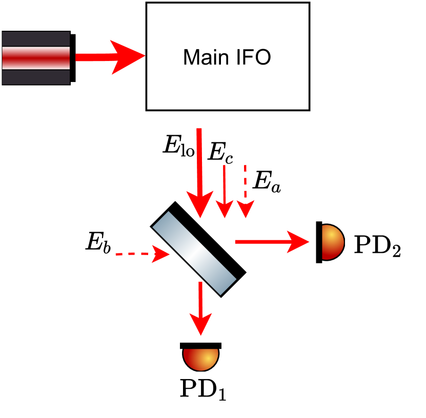
For aLIGO, the signal field leaving the interferometer’s anti-symmetric port is split on to two different PDs as shown in Figure 1. In a semiclassical way, we can write the power fluctuation on each PD as
| (1) |
where the fields are defined as in Figure 1. Specifically, is a local-oscillator field produced by an intentional detuning of the differential arm length (which is known as the “DC readout scheme” [32]). The field corresponds to vacuum fluctuations entering the interferometer from the anti-symmetric port and then returning to the readout PDs. Its interference with produces the quantum shot noise limiting a ground-based detector’s high-frequency sensitivity. As we split the signal onto two different PDs, another vacuum field enters from the open port of the beamsplitter and it carries the same amount of fluctuation as the field when there is no squeezing. Lastly, the field is produced by classical differential arm length changes. At frequency , classical noises (e.g., coating thermal noise and gas phase noise) are expected to be small, and therefore is significant only when a high-frequency GW signal is present. The transfer function from a GW strain signal at frequency to the power fluctuation is given by the interferometer’s optical response. It reads [1]
| (2) |
where , , and are, respectively, the arm length, the laser wavelength, and the input power. The factor of 2 before is because the GW signal is readout from the SUM channel . The factors and are the power buildup factors in the arm and power-recycling cavities, respectively. We further define
| (3) |
where and are the amplitude transmissivities of the input test mass and the signal-recycling mirror, and the reflectivities are given by when the optical losses are small. For aLIGO with an arm length of , we further have and . This leads to
| (4) |
where is the coupled-cavity pole frequency and . Note that Eq. (4) reduces to the expression derived in Ref. [1]. For the future generation of GW detectors like the Cosmic Explorer (CE; [33, 34, 35]) with , the approximation breaks down and therefore the full expression, Eq. (2), is used with the term given by Ref. [36] (as done in noise budgeting codes like pygwinc 111https://git.ligo.org/gwinc/pygwinc).
If we denote the power spectral density (PSD) of as (whose expectation is and units are ), then the PSD of the SUM channel due to the quantum shot noise (i.e., without ) is , and the PSD of the shot noise in terms of the GW strain can be obtained by . Similarly, we can define a NULL channel as and its PSD is .
As shown in Ref. [1], we can get rid of the quantum shot noise through a quantum-correlation technique. Specifically, we compute the real part of the cross spectral density (CSD) of and , which we denote as , and its expectation is given by
| (5) |
We thus see the shot noise is removed in the CSD and we are left with only the classical length changes of the interferometer, . On the other hand, we note the cancellation is done in the expectation. For a specific realization of (i.e., a pixel in the spectrogram or the map), the variance is given by
| (6) |
The signal-to-noise ratio (SNR) of each pixel is thus
| (7) |
This is similar to how the SNR is defined in the case of two-interferometer correlation [25]. Note that the SNR is inversely proportional to the PSD of the shot noise (which has a unit of ).
In fact, one can also remove the shot noise in expectation by computing the PSD of the NULL channel and then subtract it from the PSD of the SUM channel,
| (8) |
The variance on each pixel is
| (9) |
We immediately see that the SNR obtained this way will be the same as the one obtained from the correlation technique.
How does the SNR of the quantum correlation technique compare with the one obtained by the cross-correlating two different interferometers (see, e.g., [25])? In the two-interferometer correlation scenario, we note that the signal’s contribution to the CSD is if we assume the two interferometers have identical configurations and signal responses. The standard deviation due to uncorrelated detector noise sources is in the CSD (assuming in the shot noise limited regime). Therefore the SNR is for two-interferometer correlation. On the other hand, if we perform quantum correlation on each interferometer individually first and then combine the SNR [Eq. (7)] in quadrature, the SNR is , which is lower than directly correlating the two interferometers’ outputs. The physical reason for this degradation is the following. As we utilize the vacuum field to cancel out the expectation of the field that causes the shot noise in the SUM channel, we inevitably introduce the fluctuations associated with to the system as well. Therefore, the SNR is degraded and this is also the reason why a appeared in the denominator of (7). Despite of the loss in the SNR, the quantum correlation technique nonetheless has a few unique advantages thanks to the fact that the signal field is produced by a single interferometer, which we will discuss in more details in Section III. Therefore, it is still interesting to consider its application in detecting astrophysical signals in Section IV.
When is squeezed and is not, we see that the shot noise does not vanish in the CSD as shown in Eq. (5). Nonetheless, we can remedy the situation by also squeezing the field such that we again have . Note that this condition is needed only in the band where the shot noise dominates. Therefore, while the field is anticipated to be squeezed in a frequency-dependent way (e.g., via a filter cavity [38, 39]), a frequency-independent squeezing source is sufficient for the field to achieve at . Therefore, quantum correlation may be used not only for the archival LIGO data where the analysis above readily applies (as it has been used to constrain classical noise sources [1, 30]), but also for future detectors like LIGO-A+ [40], LIGO-Voyager [41, 42], LIGO-HF [43], the Neutron Star Extreme Matter Observatory [44], the Einstein Telescope [45, 46, 47, 48], and CE [33, 34, 35] if an additional squeezed vacuum source would be installed for field so that . We will assume this to be the case when applying quantum correlation for future detectors.
III Comparison with two-interferometer correlation
Conceptually, we note quantum correlation is largely similar to the technique of cross-correlating two different interferometers [25]. They both utilize the fact that the signal is correlated among different readout channels whereas the noise is uncorrelated. Compared to two-interferometer correlation, quantum correlation has the drawback that it only removes the quantum shot noise. And even in the shot-noise limited band, its sensitivity is slightly degraded due to the introduction of a new vacuum field into the system [which leads to the factor in the denominator in Eq. (7)]. Nonetheless, quantum correlation has a few unique advantages thanks to the fact that it requires only a single interferometer.
First of all, a single detector naturally means a higher duty cycle compared to coincident observation between at least a pair of interferometers as required by the two-interferometer correlation. For instance, during the third observing run, each LIGO detector achieved a duty cycle of individually, and the joint observation covered of the time [30]. A higher duty cycle means that it is less likely for us to miss an astrophysical signal especially if the signal is transient in nature. Quantum correlation can thus be a critical backup plan for methods originally requiring two interforemeters in case that only one detector is online during a GW event.
Quantum correlation could also make searches for GW events more efficient, as to detect a signal from a single detector, one does not need to know the source’s sky location.
To see this advantage, we first briefly review the basics to perform two-interferometer correlations [29, 25]. Note that the GW strain observed by an interferometer can be written as
| (10) |
where is the waveform in the polarization, is the antenna response of interferometer to each polarization and it depends on the sky location of the source and the polarization angle . We further use to denote the time when the GW wavefront arriving at a reference point and the time for the wave to propagate from the reference to detector . To perform two-interferometer correlation, one would need to account for the difference in a signal’s arrival time and antenna responses in interferometers and , by applying a correction factor to align their outputs [25]
| (11) |
where is the time delay of the signal in different detectors. It can be further evaluated as , where is the difference in position vectors of detectors and . For a source either with unknown location or poorly localized, we need to search over a large portion of the sky in order to perform cross-correlation between two interferometers. This could be a task computationally expensive.
For quantum correlation, this correction is not needed as the signal will reach the two readout PDs at effectively the same time (as ) and the antenna response can be absorbed into an effective distance [12]. As a result, we would only need to search over the intrinsic source parameters, thereby reducing the computational cost. Note, however, that this does not mean we discard the information on the source’s sky location. If we can detect the signal in two different interferometers, we can then readout the time delay between the interferometers as well as the difference in the SNR to infer the source’s sky position. In other words, the sky location is inferred after the GW event’s detection. Alternatively, we can also use quantum correlation as a first step to achieve the detection and to constrain the intrinsic source parameters, and then follow it up with more sensitive yet more computationally expensive analyses.
Yet another advantage of quantum correlation is that it works for polarized signals. Imagine an extreme example. If interferormeter is sensitive only to the -polarization and only to the -polarization (, ), then the cross-correlation between the two would not be able to detect a polarized signal with only the component. Nonetheless, with quantum correlation, we would at least be able to detect the signal in interferometer .
Given these advantages, we investigate how quantum correlation may help us detect astrophysical GW signals in the following section.
IV Astrophysical applications
Quantum correlation enables removing the shot noise but not classical noise, it is mostly valuable for the detection of various GW signals related to NSs at shot-noise limited frequencies, or for ground-based GW observatories. In particular, quantum correlation could potentially help the detection of post-merger bursts of BNS events with short () or intermediate duration (Secs. IV.1 and IV.2), as well as persistent or continuous GW emission from unknown pulsars (Section IV.3).
As our focus is to detect the signal and extract the intrinsic parameters using a single detector, we will fix the source to have a face-on orientation and an antenna response for the cases in Secs. IV.1 and IV.2. Changing the source’s orientation, sky location, and polarization only affects the overall amplitude of the signal. Note, however, that these extrinsic parameters (such as the source’s sky location) can be extract after the detection has been made in multiple detectors, though we deferred the analysis on extrinsic parameters to future studies.
IV.1 Short-duration bursts
It has been postulated that if a BNS’s total mass exceeds a maximum value allowed by a uniformly rotating star, its post-merger remnant could be a hypermassive NS that collapse in less than a second [49, 15]. GW170817 [50], for example, is likely to have a total mass that can lead to a hypermassive NS [15, 51, 17].
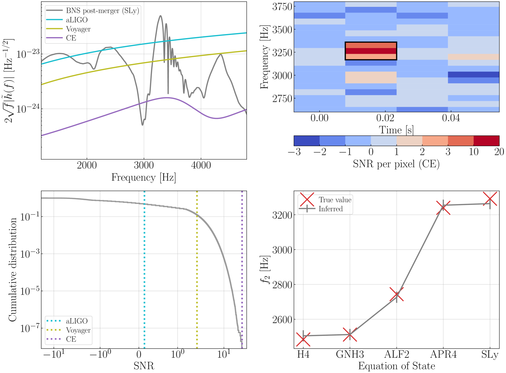
The associated GW waveform of a hypermassive NS has been extensively studied by the literature (see, e.g., Refs. [52, 53, 54, 55, 56, 57, 58]). For the analysis here, we take GW waveforms provide in [53, 54, 55]. The comparison between the GW signal (the gray curve) and the shot noise level of representative detectors (colored curves) are shown in the top-left panel in Fig. 2. We use cyan, olive, and purple to respectively represent aLIGO, Voyager, and CE and this convention will be used throughout this Section. We place the merger at a distance of and assume the SLy equation of state [59]. The waveform is filtered the same way as described in Ref. [54] to remove the pre-merger part.
To perform the quantum correlation measurement, we convert the strain signal to power fluctuations on the PDs using Eq. (2) and superpose it with the other noise sources (dominated by the quantum shot noise in the band of interest). We then normalize each pixel by the standard deviation [Eq. 6]. A resultant normalized -map is presented in the top-right panel of Figure 2. In this example, the merger happens at .
To detect the signal, we consider detection boxes with a size of , corresponding to three pixels in the -map (see, e.g., the black box in the top-right panel of Figure 2). The cumulative distribution of the total SNR in many realizations of signal-free boxes is further shown in the lower-left panel of Figure 2, serving as the background statistics for us to construct the detection threshold. Simulations here are performed over simulated Gaussian noises. Also shown in the vertical lines are the expected SNR inside the detection box of the signal shown in the top-left panel in various detectors.
Following Ref. [15], we define the root-sum-squared strain amplitude as
| (12) |
where are the Fourier transforms of . The efficiency of the algorithm is then analyzed in terms of the minimum required in order to make the false-alarm probability (FAP) lower than a certain threshold. Because our detection box is about 100 times shorter than the one used in Ref. [15], we thus choose a threshold of which is 100 times lower than the threshold used in Ref. [15]. This leads to , , and for the short-duration post-merger signal to be detected by aLIGO, Voyager, and CE, respectively. If we instead choose a more strict detection threshold of , this only increases the value of by .
Besides detecting the signal itself, it is also of great significance to constrain the peak frequency of the post-merger signal. This is also known as the frequency following the convention used in Ref. [55] and it has been shown to contain critical information of the NS equation of state [60]. The peak frequency can be constrained from the -map by computing the SNR-weighted-mean frequency of the detection box that has the maximum SNR.
In the bottom-right panel of Fig. 2, we compare the inferred frequency (gray pluses) and the true frequency for a variety of NS equation of states, covering hard (H4 [61]; GNH3 [62]), intermediate (ALF2 [63]), and soft (APR4 [64]; SLy [59]) ones. In all the cases, we keep the source at 100 Mpc and assume CE’s sensitivity in the detector. We find the fluctuation in the inferred value due to different noise realization is small and the uncertainty in the inference is set by the resolution of the pixel. For all the equation of states we consider, the difference between the inferred value and the true one is less than half of the pixel’s size, or , which we adopt as the size of the error bar when generating the gray markers in the plot. It is thus possible for us to use quantum correlation and future detectors to distinguish hard, intermediate, and soft equation of states.
IV.2 Intermediate-duration bursts
For less massive BNS mergers, the remnant could be a supermassive NS whose mass is greater than the maximum value for a non-rotating NS. In this case, the GW signal could have a long duration, ranging from to [65].
Following Refs. [15, 16], here we consider the possibility that the merger produces a fast-spinning magnetar [66]. The subsequent spinning down of the magnetar follows a trajectory [67]
| (13) |
where is an initial GW frequency, is the spin-down timescale, and is the braking index. The phase of the GW waveform is then given by
| (14) |
and the overall amplitude [67]
| (15) |
where , , and are respectively the ellipticity, moment of inertia of the NS, and the distance to the source.
Consistent with Ref. [15], we adopt to describe the spin-down trajectory. To set the amplitude, we further use , , and .
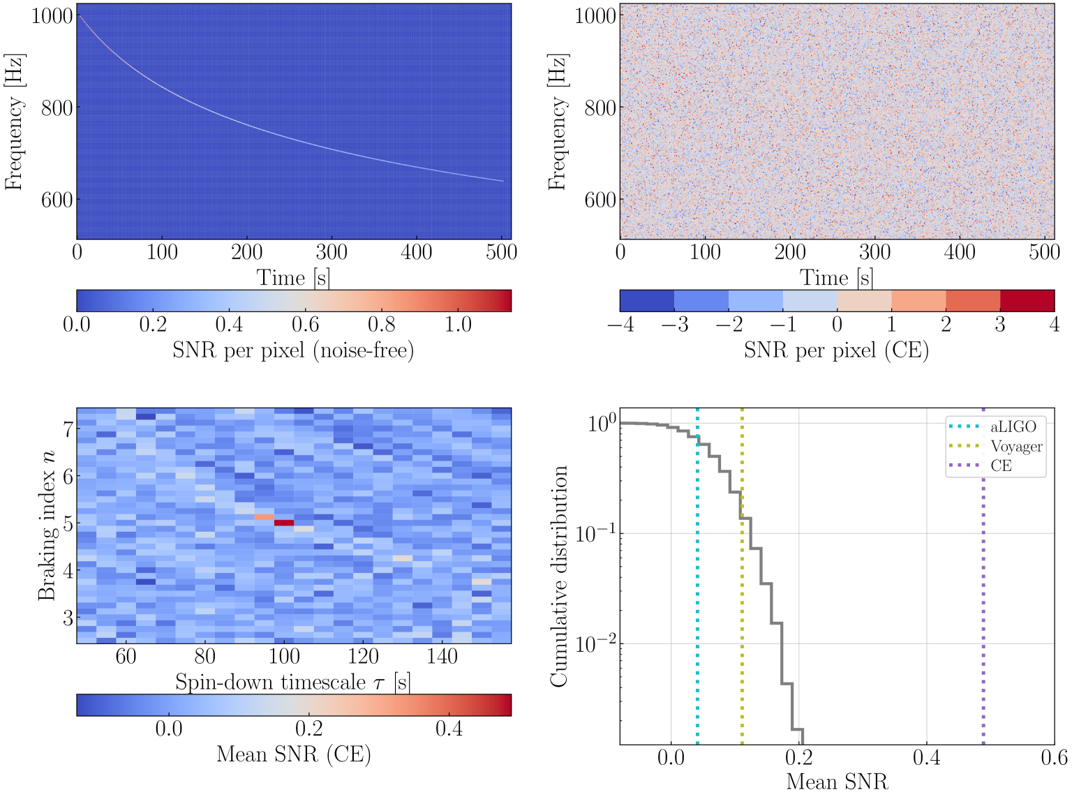
The signal (normalized by ) is shown in the top-left panel of Fig. 3 and its superposition with detector noise (assuming CE’s sensitivity) is shown in the top-right panel. Here the -map has a pixel size of .
While the signal is too weak to be directly visible by eyes, it can nonetheless be detected if we search for excess power along certain trajectories including hundreds of pixels. Generic clustering and pattern-recognition algorithms (e.g., Refs. [68, 69, 70, 71]) can be applied, yet as a proof-of-concept study, here we simply search over trajectories specified by Eq. (13) but with varying parameters. Each trajectory we search spans 500 pixels.
The resultant mean SNR along different trajectories is shown in the bottom left panel of Figure 3. When we hit the right parameters describing the signal, we note a sudden increase in the mean SNR along the trajectory. This allow us to simultaneously detect the signal and constrain its properties.
To quantitatively establish the sensitivity, we consider the cumulative distribution of the mean SNR along signal-free trajectories. The vertical lines represent the expected SNR of the signal (top-left panel of Figure 3) in different detectors. If we choose an as the detection threshold (which is consistent with Ref. [15]), this leads to , , and for aLIGO, Voyager, and CE, respectively.
IV.3 Continuous-wave sources
Besides bursts, quantum correlation could potentially contribute to the search for GW emission from fast-rotating pulsars (see, e.g., [72, 73, 74]).
Suppose the total duration of observation is . We divide the data into non-overlapping segments, and each segment has a duration of . We perform fast Fourier transfer on each segment of data and compute the corresponding CSD for quantum correlation. The expected noise in the averaged CSD over segments is approximated by the quadratic sum of the variance in the shot noise [Eq. (6)] and the nonvanishing classical noise ,
| (16) |
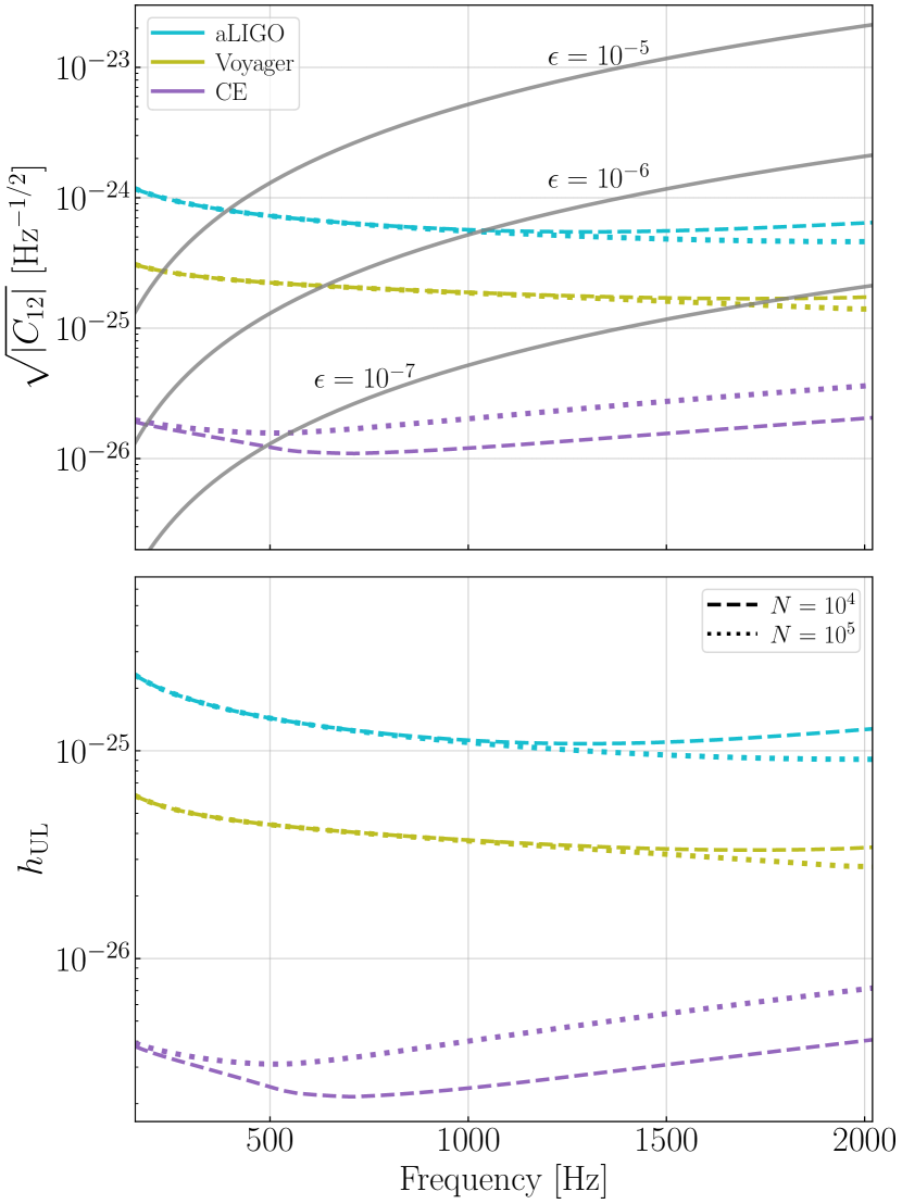
The resultant noise level is shown in the top panel in Figure 4. We use dashed (dotted) lines to represent the estimated noise level after averaging over () segments. For aLIGO and Voyager, about averages will be sufficient to reach the noise floor set by classical noise sources such as thermal noise 222For simplicity, we consider here only the broadband classical noise and ignore sharp lines in the spectra. that cannot be removed by quantum correlation here. This corresponds to if . For CE, the classical-noise floor is significantly lower, and even with averages ( years for ), the sensitivity is still limited by the term at 1000 Hz.
The noise level is to be compared with the expected signal strength in the CSD which we show in the solid lines for different values of ellipticities. The amplitude of the wave can still be computed from Eq. (15). We fix and place the source at an averaged effective distance of . For a monochromatic GW emission with amplitude at frequency , we have
| (17) |
Depending on the value of (and hence the frequency resolution in the CSD), the Doppler effect due to the revolution of the Earth around the Sun and the revolution of the pulsar itself if it is in a binary system can cause the signal to drift in multiple frequency bins. As a proof-of-concept study, we ignore here the complication due to the Doppler shift as it can be readily corrected for with existing algorithms such as FrequencyHough [76] (we would need to include the sky location of the source as search parameters here). Under this assumption, upper limits on the GW strain can then be obtained as (cf. eq. (6) in Ref. [74]; see also Ref. [76])
| (18) |
where is a threshold SNR to claim a detection (note our definition of SNR follows Ref. [25] and is defined in terms of power instead of amplitude as used in Ref. [76]). Depending on whether is limited by or [Eq. (16)], scales with as or for given . In both cases, longer segment length is preferred. The upper limits are shown in the bottom panel of Fig. 4. Consistent with Ref. [74], we have assumed . We also adopted a fiducial detection threshold of .
Note that when applied to the detection of continuous GW emissions, quantum correlation provides a way to find hot pixels in the -map, which can then be fed to the FrequencyHough algorithm [76] as inputs. It thus complements the existing methods such as using the auto-regressive estimation as proposed in Ref. [77]. While quantum correlation does not enhance the fundamental sensitivity, we could potentially benefit from its simplicity in removing the expectation value of the shot noise. Moreover, it naturally handles fluctuations and nonstationarities in the interferometer (as is a common reference field when computing and ; see the discussion in Section V). Though as a caveat, to reach the full sensitivity of quantum correlation, it requires the system to be well balanced. We will discuss this point more in Section V.
V Conclusion and discussion
In this work, we explored the possibility of detecting astrophysical GW events using quantum correlation, a technique that has been used by the LIGO instrumentation group to constrain classical noise in the LIGO interferometers [1, 30]. We analyzed in a generic context the sensitivity of the technique in Sec. II. The main advantage of quantum correlation is that it requires only a single interferometer for the detection (Sec. III), which naturally leads to a higher duty cycle compared to two-interferometer correlation. Moreover, the signals captured by the two PDs in quantum correlation (Fig. 1) will share the same antenna response and arrival time, and consequently the detection search can be made more efficient as we do not need to search over extrinsic parameters like the sky location of the event to align the signals (at least for burst signals where the Doppler effect due to Earth’s revolution and rotation can be ignored). This also allows us to detect highly polarized GW signals with quantum correlation. We then considered a few specific examples of using this technique to detect high-frequency GW signals in Sec. IV, including BNS post-merger remnants with both short- (; Sec. IV.1) and intermediate (; Sec. IV.2) duration, as well as continuous GW emissions from pulsars (especially those at high GW frequencies; Sec. IV.3).
Conceptually, the quantum correlation technique can be understood in analogy to the correlation between two different interferometers (Sec. III). The quantum shot noise is uncorrelated among the two PDs reading out the GW signal (Fig. 1), thereby allowing its removal via cross-correlation. This allows us to adopt results developed for analysing the cross-correlation between different interferometers. Indeed, our definition of the SNR for each pixel [Eq. (7)] follows closely Ref. [25], and multiple pattern recognition algorithms [68, 69] can be readily applied to search for the signal in the -map.
Meanwhile, Eq. (5) suggests that we can also view the quantum correlation as follows. By introducing the new field , it provides us an estimation of (as ), thereby allowing the removal of its expectation value in the (cross-)spectra. This further suggests that if we know , we may also directly subtract it out and detect the GW signal as excess power in the residual spectra. In practice, to do the direct subtraction one would need to take into account the nonstationarity in the interferometer, which could mean extra complications compared to performing quantum correlation. For example, to directly predict the value of , one would need to know the instantaneous value of the local-oscillator field , whereas the fluctuations in do not affect the quantum correlation because it serves as a common reference when computing and . Nevertheless, doing the direct subtraction is an interesting direction to be explored by future studies as it might improve the sensitivity by avoiding the introduction of the uncertainties in , which degrades the SNR in Eq. (5) by . To tackle the nonstationarities in the interferometer, one could utilize auxiliary channels in LIGO [78, 79]. Furthermore, with auxiliary channels one could predict not only the expected spectrum of the quantum shot noise but also other noise sources across the entire spectra. We plan to explore this possibility in follow-up studies.
We note that the quantum correlation may pick up instrumental glitches as hot pixels in the CSD. Nonetheless, there are at least two ways to distinguish between terrestrial glitches and astrophysical signals. One is to look for coincidence of hot pixels in multiple detectors. Indeed, this is how we can extract sky location of the source under the quantum correlation technique. On the other hand, if we only find a signal candidate in a single detector, it may still have an astrophysical origin as its disappearance in the other detector(s) might be due to unfavorable antenna response. In this case, we can still veto instrumental glitches utilizing auxiliary channels as routinely done for the LIGO detector characterization [80, 81, 82].
For quantum correlation, uncertainties in the interferometer calibration [83, 84] do not significantly affect the detection. This is because the signal is detected as excess power, which further means the phase of the signal is not used and the amplitude can be measured directly in terms of raw power in the readout PDs to establish the detection statistics. The calibration from power in the PDs to the astrophysical strain will affect mostly the subsequent inference of source parameters such as its distance and ellipticity yet less the detection of the signal itself.
As a proof-of-principle study, we have assumed the final beamsplitter shown in Figure 1 is an ideal 50-50 beamsplitter, and when squeezed vacuum is used, we have assumed the squeezing level of the field matches exactly the field. In reality, imbalance exists inevitably, which can potentially degrade the performance of the quantum correlation technique. One way to set the tolerance on the imbalance between the beamsplitter’s transmissivity and reflectivity and the mismatch of squeezing levels for different squeezers is by requiring [cf. Eq. (16)]
| (19) |
For aLIGO, the requirement is set by the term, and satisfying the condition at 1,000 Hz means the difference in and needs to be . For CE, is significantly lower compared to the shot noise and the requirement is set by the number of averages . In this case, the mismatch needs to be for . While failing to meet the requirement above will degrade the sensitivity to continuous-wave emission as discussed in Section IV.3, it does not significantly hinder the sensitivity to burst signals (Secs. IV.1 and IV.2). For detecting the burst signals, the requirement is set by
| (20) |
where is the number of pixels along a detection trajectory. Since we typically have for burst signals, we have especially for future detectors like CE. This leads to a more feasible requirement on the mismatch to be .
Acknowledgements.
We thank the helpful comments and feedback from L. Sun, K. Riles and other LVK colleagues. H.Y. is supported by the Sherman Fairchild Foundation. D.M. acknowledges the support of the Institute for Gravitational Wave Astronomy at the University of Birmingham, STFC (Grant No. ST/T006609/1, ST/S000305/1), and EPSRC research councils (Grant No. EP/V048872/1, EP/V008617/1). R.X.A is supported by NSF Grants No. PHY-1764464 and PHY-1912677. Y.C. is supported by the Simons Foundation (Award Number 568762) and by NSF Grants PHY-2011961, PHY-2011968, PHY–1836809.References
- Martynov et al. [2017] D. V. Martynov, V. V. Frolov, S. Kandhasamy, K. Izumi, H. Miao, N. Mavalvala, E. D. Hall, R. Lanza, and et al., Quantum correlation measurements in interferometric gravitational-wave detectors, Phys. Rev. A 95, 043831 (2017), arXiv:1702.03329 [physics.optics] .
- Abbott et al. [2019] B. P. Abbott, R. Abbott, T. D. Abbott, S. Abraham, F. Acernese, K. Ackley, C. Adams, R. X. Adhikari, V. B. Adya, C. Affeldt, LIGO Scientific Collaboration, and Virgo Collaboration, GWTC-1: A Gravitational-Wave Transient Catalog of Compact Binary Mergers Observed by LIGO and Virgo during the First and Second Observing Runs, Physical Review X 9, 031040 (2019), arXiv:1811.12907 [astro-ph.HE] .
- LIGO Scientific Collaboration et al. [2021] LIGO Scientific Collaboration, Virgo Collaboration, and et al., GWTC-2: Compact Binary Coalescences Observed by LIGO and Virgo during the First Half of the Third Observing Run, Physical Review X 11, 021053 (2021), arXiv:2010.14527 [gr-qc] .
- The LIGO Scientific Collaboration et al. [2021] The LIGO Scientific Collaboration, the Virgo Collaboration, the KAGRA Collaboration, and et al., GWTC-3: Compact Binary Coalescences Observed by LIGO and Virgo During the Second Part of the Third Observing Run, arXiv e-prints , arXiv:2111.03606 (2021), arXiv:2111.03606 [gr-qc] .
- Venumadhav et al. [2020] T. Venumadhav, B. Zackay, J. Roulet, L. Dai, and M. Zaldarriaga, New binary black hole mergers in the second observing run of Advanced LIGO and Advanced Virgo, Phys. Rev. D 101, 083030 (2020), arXiv:1904.07214 [astro-ph.HE] .
- Olsen et al. [2022] S. Olsen, T. Venumadhav, J. Mushkin, J. Roulet, B. Zackay, and M. Zaldarriaga, New binary black hole mergers in the LIGO–Virgo O3a data, arXiv e-prints , arXiv:2201.02252 (2022), arXiv:2201.02252 [astro-ph.HE] .
- Aasi et al. [2015] J. Aasi et al. (LIGO Scientific), Advanced LIGO, Class. Quant. Grav. 32, 074001 (2015), arXiv:1411.4547 [gr-qc] .
- Acernese et al. [2015] F. Acernese et al. (VIRGO), Advanced Virgo: a second-generation interferometric gravitational wave detector, Class. Quant. Grav. 32, 024001 (2015), arXiv:1408.3978 [gr-qc] .
- Kagra Collaboration and et al. [2019] Kagra Collaboration and et al., KAGRA: 2.5 generation interferometric gravitational wave detector, Nature Astronomy 3, 35 (2019), arXiv:1811.08079 [gr-qc] .
- Kagra Collaboration and et al. [2021] Kagra Collaboration and et al., Overview of KAGRA: Detector design and construction history, Progress of Theoretical and Experimental Physics 2021, 05A101 (2021), arXiv:2005.05574 [physics.ins-det] .
- Cannon et al. [2010] K. Cannon, A. Chapman, C. Hanna, D. Keppel, A. C. Searle, and A. J. Weinstein, Singular value decomposition applied to compact binary coalescence gravitational-wave signals, Phys. Rev. D 82, 044025 (2010), arXiv:1005.0012 [gr-qc] .
- Allen et al. [2012] B. Allen, W. G. Anderson, P. R. Brady, D. A. Brown, and J. D. E. Creighton, FINDCHIRP: An algorithm for detection of gravitational waves from inspiraling compact binaries, Phys. Rev. D 85, 122006 (2012), arXiv:gr-qc/0509116 [gr-qc] .
- Messick et al. [2017] C. Messick, K. Blackburn, P. Brady, P. Brockill, K. Cannon, R. Cariou, S. Caudill, S. J. Chamberlin, J. D. E. Creighton, R. Everett, C. Hanna, D. Keppel, R. N. Lang, T. G. F. Li, D. Meacher, A. Nielsen, C. Pankow, S. Privitera, H. Qi, S. Sachdev, L. Sadeghian, L. Singer, E. G. Thomas, L. Wade, M. Wade, A. Weinstein, and K. Wiesner, Analysis framework for the prompt discovery of compact binary mergers in gravitational-wave data, Phys. Rev. D 95, 042001 (2017), arXiv:1604.04324 [astro-ph.IM] .
- Venumadhav et al. [2019] T. Venumadhav, B. Zackay, J. Roulet, L. Dai, and M. Zaldarriaga, New search pipeline for compact binary mergers: Results for binary black holes in the first observing run of Advanced LIGO, Phys. Rev. D 100, 023011 (2019), arXiv:1902.10341 [astro-ph.IM] .
- Abbott and et al. [2017] B. P. Abbott and et al., Search for Post-merger Gravitational Waves from the Remnant of the Binary Neutron Star Merger GW170817, ApJ 851, L16 (2017), arXiv:1710.09320 [astro-ph.HE] .
- LIGO Scientific Collaboration et al. [2019a] LIGO Scientific Collaboration, Virgo Collaboration, and et al., Search for Gravitational Waves from a Long-lived Remnant of the Binary Neutron Star Merger GW170817, ApJ 875, 160 (2019a), arXiv:1810.02581 [gr-qc] .
- LIGO Scientific Collaboration et al. [2019b] LIGO Scientific Collaboration, Virgo Collaboration, and et al., Properties of the Binary Neutron Star Merger GW170817, Physical Review X 9, 011001 (2019b), arXiv:1805.11579 [gr-qc] .
- Ligo Scientific Collaboration et al. [2021a] Ligo Scientific Collaboration, VIRGO Collaboration, Kagra Collaboration, and et al., All-sky search for long-duration gravitational-wave bursts in the third Advanced LIGO and Advanced Virgo run, Phys. Rev. D 104, 102001 (2021a), arXiv:2107.13796 [gr-qc] .
- Ligo Scientific Collaboration et al. [2021b] Ligo Scientific Collaboration, VIRGO Collaboration, Kagra Collaboration, and et al., All-sky search for short gravitational-wave bursts in the third Advanced LIGO and Advanced Virgo run, Phys. Rev. D 104, 122004 (2021b), arXiv:2107.03701 [gr-qc] .
- van Putten et al. [2019] M. H. P. M. van Putten, A. Levinson, F. Frontera, C. Guidorzi, L. Amati, and M. Della Valle, Prospects for multi-messenger extended emission from core-collapse supernovae in the Local Universe, European Physical Journal Plus 134, 537 (2019), arXiv:1709.04455 [astro-ph.HE] .
- van Putten [2001] M. H. van Putten, Proposed Source of Gravitational Radiation from a Torus around a Black Hole, Phys. Rev. Lett. 87, 091101 (2001), arXiv:astro-ph/0107007 [astro-ph] .
- Huerta et al. [2018] E. A. Huerta, C. J. Moore, P. Kumar, D. George, A. J. K. Chua, R. Haas, E. Wessel, D. Johnson, D. Glennon, A. Rebei, A. M. Holgado, J. R. Gair, and H. P. Pfeiffer, Eccentric, nonspinning, inspiral, Gaussian-process merger approximant for the detection and characterization of eccentric binary black hole mergers, Phys. Rev. D 97, 024031 (2018), arXiv:1711.06276 [gr-qc] .
- LIGO Scientific Collaboration et al. [2019c] LIGO Scientific Collaboration, Virgo Collaboration, and et al. (LIGO Scientific, Virgo), Search for Eccentric Binary Black Hole Mergers with Advanced LIGO and Advanced Virgo during their First and Second Observing Runs, Astrophys. J. 883, 149 (2019c), arXiv:1907.09384 [astro-ph.HE] .
- Klimenko et al. [2016] S. Klimenko, G. Vedovato, M. Drago, F. Salemi, V. Tiwari, G. A. Prodi, C. Lazzaro, K. Ackley, S. Tiwari, C. F. Da Silva, and G. Mitselmakher, Method for detection and reconstruction of gravitational wave transients with networks of advanced detectors, Phys. Rev. D 93, 042004 (2016), arXiv:1511.05999 [gr-qc] .
- Thrane et al. [2011] E. Thrane, S. Kandhasamy, C. D. Ott, W. G. Anderson, N. L. Christensen, M. W. Coughlin, S. Dorsher, S. Giampanis, V. Mandic, A. Mytidis, T. Prestegard, P. Raffai, and B. Whiting, Long gravitational-wave transients and associated detection strategies for a network of terrestrial interferometers, Phys. Rev. D 83, 083004 (2011), arXiv:1012.2150 [astro-ph.IM] .
- Sutton et al. [2010] P. J. Sutton, G. Jones, S. Chatterji, P. Kalmus, I. Leonor, S. Poprocki, J. Rollins, A. Searle, L. Stein, M. Tinto, and M. Was, X-Pipeline: an analysis package for autonomous gravitational-wave burst searches, New Journal of Physics 12, 053034 (2010), arXiv:0908.3665 [gr-qc] .
- Cornish and Littenberg [2015] N. J. Cornish and T. B. Littenberg, Bayeswave: Bayesian inference for gravitational wave bursts and instrument glitches, Classical and Quantum Gravity 32, 135012 (2015), arXiv:1410.3835 [gr-qc] .
- Cornish et al. [2021] N. J. Cornish, T. B. Littenberg, B. Bécsy, K. Chatziioannou, J. A. Clark, S. Ghonge, and M. Millhouse, BayesWave analysis pipeline in the era of gravitational wave observations, Phys. Rev. D 103, 044006 (2021), arXiv:2011.09494 [gr-qc] .
- Allen and Romano [1999] B. Allen and J. D. Romano, Detecting a stochastic background of gravitational radiation: Signal processing strategies and sensitivities, Phys. Rev. D 59, 102001 (1999), arXiv:gr-qc/9710117 [gr-qc] .
- Buikema et al. [2020] A. Buikema, C. Cahillane, G. L. Mansell, C. D. Blair, and et al., Sensitivity and performance of the advanced ligo detectors in the third observing run, Phys. Rev. D 102, 062003 (2020).
- Tse et al. [2019] M. Tse, H. Yu, N. Kijbunchoo, A. Fernandez-Galiana, P. Dupej, L. Barsotti, C. D. Blair, D. D. Brown, and et al., Quantum-Enhanced Advanced LIGO Detectors in the Era of Gravitational-Wave Astronomy, Phys. Rev. Lett. 123, 231107 (2019).
- Fricke et al. [2012] T. T. Fricke, N. D. Smith-Lefebvre, R. Abbott, R. Adhikari, K. L. Dooley, M. Evans, P. Fritschel, V. V. Frolov, K. Kawabe, J. S. Kissel, B. J. J. Slagmolen, and S. J. Waldman, DC readout experiment in Enhanced LIGO, Classical and Quantum Gravity 29, 065005 (2012), arXiv:1110.2815 [physics.ins-det] .
- Abbott et al. [2017a] B. P. Abbott, R. Abbott, T. D. Abbott, M. R. Abernathy, K. Ackley, C. Adams, P. Addesso, R. X. Adhikari, V. B. Adya, C. Affeldt, and et al., Exploring the sensitivity of next generation gravitational wave detectors, Classical and Quantum Gravity 34, 044001 (2017a), arXiv:1607.08697 [astro-ph.IM] .
- Reitze et al. [2019] D. Reitze, R. X. Adhikari, S. Ballmer, B. Barish, L. Barsotti, G. Billingsley, D. A. Brown, Y. Chen, D. Coyne, R. Eisenstein, M. Evans, P. Fritschel, E. D. Hall, A. Lazzarini, G. Lovelace, J. Read, B. S. Sathyaprakash, D. Shoemaker, J. Smith, C. Torrie, S. Vitale, R. Weiss, C. Wipf, and M. Zucker, Cosmic Explorer: The U.S. Contribution to Gravitational-Wave Astronomy beyond LIGO, in Bulletin of the American Astronomical Society, Vol. 51 (2019) p. 35, arXiv:1907.04833 [astro-ph.IM] .
- Evans et al. [2021] M. Evans, R. X. Adhikari, C. Afle, S. W. Ballmer, S. Biscoveanu, S. Borhanian, D. A. Brown, Y. Chen, and et al., A Horizon Study for Cosmic Explorer: Science, Observatories, and Community, arXiv e-prints , arXiv:2109.09882 (2021), arXiv:2109.09882 [astro-ph.IM] .
- Schilling [1997] R. Schilling, Angular and frequency response of LISA, Classical and Quantum Gravity 14, 1513 (1997).
- Note [1] https://git.ligo.org/gwinc/pygwinc.
- McCuller et al. [2020] L. McCuller, C. Whittle, D. Ganapathy, K. Komori, M. Tse, A. Fernandez-Galiana, L. Barsotti, P. Fritschel, M. MacInnis, F. Matichard, K. Mason, N. Mavalvala, R. Mittleman, H. Yu, M. E. Zucker, and M. Evans, Frequency-Dependent Squeezing for Advanced LIGO, Phys. Rev. Lett. 124, 171102 (2020), arXiv:2003.13443 [astro-ph.IM] .
- Zhao et al. [2020] Y. Zhao, N. Aritomi, E. Capocasa, M. Leonardi, M. Eisenmann, Y. Guo, E. Polini, A. Tomura, and et al., Frequency-Dependent Squeezed Vacuum Source for Broadband Quantum Noise Reduction in Advanced Gravitational-Wave Detectors, Phys. Rev. Lett. 124, 171101 (2020), arXiv:2003.10672 [astro-ph.IM] .
- Kagra Collaboration et al. [2018] Kagra Collaboration, LIGO Scientific Collaboration, and VIRGO Collaboration, Prospects for observing and localizing gravitational-wave transients with Advanced LIGO, Advanced Virgo and KAGRA, Living Reviews in Relativity 21, 3 (2018), arXiv:1304.0670 [gr-qc] .
- Adhikari et al. [2017] R. Adhikari, N. Smith, A. Brooks, and et al., Ligo voyager upgrade concept (2017), LIGO Document T1400226.
- Adhikari et al. [2020] R. X. Adhikari, K. Arai, A. F. Brooks, C. Wipf, and et al., A cryogenic silicon interferometer for gravitational-wave detection, Classical and Quantum Gravity 37, 165003 (2020), arXiv:2001.11173 [astro-ph.IM] .
- Martynov et al. [2019] D. Martynov, H. Miao, H. Yang, F. H. Vivanco, E. Thrane, R. Smith, P. Lasky, W. E. East, R. Adhikari, A. Bauswein, A. Brooks, Y. Chen, T. Corbitt, A. Freise, H. Grote, Y. Levin, C. Zhao, and A. Vecchio, Exploring the sensitivity of gravitational wave detectors to neutron star physics, Phys. Rev. D 99, 102004 (2019), arXiv:1901.03885 [astro-ph.IM] .
- Ackley et al. [2020] K. Ackley, V. B. Adya, P. Agrawal, P. Altin, G. Ashton, M. Bailes, E. Baltinas, A. Barbuio, and et al., Neutron Star Extreme Matter Observatory: A kilohertz-band gravitational-wave detector in the global network, PASA 37, e047 (2020), arXiv:2007.03128 [astro-ph.HE] .
- Hild et al. [2010] S. Hild, S. Chelkowski, A. Freise, J. Franc, N. Morgado, R. Flaminio, and R. DeSalvo, A xylophone configuration for a third-generation gravitational wave detector, Classical and Quantum Gravity 27, 015003 (2010), arXiv:0906.2655 [gr-qc] .
- Punturo et al. [2010] M. Punturo, M. Abernathy, F. Acernese, B. Allen, N. Andersson, K. Arun, F. Barone, B. Barr, and et al., The third generation of gravitational wave observatories and their science reach, Classical and Quantum Gravity 27, 084007 (2010).
- Hild et al. [2011] S. Hild, M. Abernathy, F. Acernese, P. Amaro-Seoane, N. Andersson, K. Arun, F. Barone, B. Barr, and et al., Sensitivity studies for third-generation gravitational wave observatories, Classical and Quantum Gravity 28, 094013 (2011), arXiv:1012.0908 [gr-qc] .
- Sathyaprakash et al. [2012] B. Sathyaprakash, M. Abernathy, F. Acernese, P. Ajith, B. Allen, P. Amaro-Seoane, N. Andersson, S. Aoudia, K. Arun, P. Astone, and et al., Scientific objectives of Einstein Telescope, Classical and Quantum Gravity 29, 124013 (2012), arXiv:1206.0331 [gr-qc] .
- Baumgarte et al. [2000] T. W. Baumgarte, S. L. Shapiro, and M. Shibata, On the Maximum Mass of Differentially Rotating Neutron Stars, ApJ 528, L29 (2000), arXiv:astro-ph/9910565 [astro-ph] .
- LIGO Scientific Collaboration et al. [2017] LIGO Scientific Collaboration, Virgo Collaboration, and et al., GW170817: Observation of Gravitational Waves from a Binary Neutron Star Inspiral, Phys. Rev. Lett. 119, 161101 (2017), arXiv:1710.05832 [gr-qc] .
- Abbott et al. [2017b] B. P. Abbott, R. Abbott, T. D. Abbott, F. Acernese, K. Ackley, C. Adams, T. Adams, P. Addesso, and et al., Gravitational Waves and Gamma-Rays from a Binary Neutron Star Merger: GW170817 and GRB 170817A, ApJ 848, L13 (2017b), arXiv:1710.05834 [astro-ph.HE] .
- Hotokezaka et al. [2013] K. Hotokezaka, K. Kiuchi, K. Kyutoku, T. Muranushi, Y.-i. Sekiguchi, M. Shibata, and K. Taniguchi, Remnant massive neutron stars of binary neutron star mergers: Evolution process and gravitational waveform, Phys. Rev. D 88, 044026 (2013), arXiv:1307.5888 [astro-ph.HE] .
- Takami et al. [2014] K. Takami, L. Rezzolla, and L. Baiotti, Constraining the Equation of State of Neutron Stars from Binary Mergers, Phys. Rev. Lett. 113, 091104 (2014), arXiv:1403.5672 [gr-qc] .
- Takami et al. [2015] K. Takami, L. Rezzolla, and L. Baiotti, Spectral properties of the post-merger gravitational-wave signal from binary neutron stars, Phys. Rev. D 91, 064001 (2015), arXiv:1412.3240 [gr-qc] .
- Rezzolla and Takami [2016] L. Rezzolla and K. Takami, Gravitational-wave signal from binary neutron stars: A systematic analysis of the spectral properties, Phys. Rev. D 93, 124051 (2016), arXiv:1604.00246 [gr-qc] .
- Kawamura et al. [2016] T. Kawamura, B. Giacomazzo, W. Kastaun, R. Ciolfi, A. Endrizzi, L. Baiotti, and R. Perna, Binary neutron star mergers and short gamma-ray bursts: Effects of magnetic field orientation, equation of state, and mass ratio, Phys. Rev. D 94, 064012 (2016), arXiv:1607.01791 [astro-ph.HE] .
- Dietrich et al. [2018] T. Dietrich, D. Radice, S. Bernuzzi, F. Zappa, A. Perego, B. Brügmann, S. Vivekanandji Chaurasia, R. Dudi, W. Tichy, and M. Ujevic, CoRe database of binary neutron star merger waveforms, Classical and Quantum Gravity 35, 24LT01 (2018), arXiv:1806.01625 [gr-qc] .
- Zappa et al. [2018] F. Zappa, S. Bernuzzi, D. Radice, A. Perego, and T. Dietrich, Gravitational-Wave Luminosity of Binary Neutron Stars Mergers, Phys. Rev. Lett. 120, 111101 (2018), arXiv:1712.04267 [gr-qc] .
- Douchin and Haensel [2001] F. Douchin and P. Haensel, A unified equation of state of dense matter and neutron star structure, A&A 380, 151 (2001), arXiv:astro-ph/0111092 [astro-ph] .
- Shibata [2005] M. Shibata, Constraining Nuclear Equations of State Using Gravitational Waves from Hypermassive Neutron Stars, Phys. Rev. Lett. 94, 201101 (2005), arXiv:gr-qc/0504082 [gr-qc] .
- Glendenning and Moszkowski [1991] N. K. Glendenning and S. A. Moszkowski, Reconciliation of neutron-star masses and binding of the Lambda in hypernuclei, Phys. Rev. Lett. 67, 2414 (1991).
- Glendenning [1985] N. K. Glendenning, Neutron stars are giant hypernuclei ?, ApJ 293, 470 (1985).
- Alford et al. [2005] M. Alford, M. Braby, M. Paris, and S. Reddy, Hybrid Stars that Masquerade as Neutron Stars, ApJ 629, 969 (2005), arXiv:nucl-th/0411016 [nucl-th] .
- Akmal et al. [1998] A. Akmal, V. R. Pandharipande, and D. G. Ravenhall, Equation of state of nucleon matter and neutron star structure, Phys. Rev. C 58, 1804 (1998), arXiv:nucl-th/9804027 [nucl-th] .
- Ravi and Lasky [2014] V. Ravi and P. D. Lasky, The birth of black holes: neutron star collapse times, gamma-ray bursts and fast radio bursts, MNRAS 441, 2433 (2014), arXiv:1403.6327 [astro-ph.HE] .
- Cutler [2002] C. Cutler, Gravitational waves from neutron stars with large toroidal B fields, Phys. Rev. D 66, 084025 (2002), arXiv:gr-qc/0206051 [gr-qc] .
- Lasky et al. [2017] P. Lasky, N. Sarin, and L. Sammut, Long-duration waveform models for millisecond magnetars born in binary neutron star mergers (2017), LIGO Document T1700408.
- Thrane and Coughlin [2013] E. Thrane and M. Coughlin, Searching for gravitational-wave transients with a qualitative signal model: Seedless clustering strategies, Phys. Rev. D 88, 083010 (2013), arXiv:1308.5292 [astro-ph.IM] .
- Thrane and Coughlin [2015] E. Thrane and M. Coughlin, Detecting Gravitation-Wave Transients at 5 : A Hierarchical Approach, Phys. Rev. Lett. 115, 181102 (2015), arXiv:1507.00537 [astro-ph.IM] .
- Sun and Melatos [2019] L. Sun and A. Melatos, Application of hidden Markov model tracking to the search for long-duration transient gravitational waves from the remnant of the binary neutron star merger GW170817, Phys. Rev. D 99, 123003 (2019), arXiv:1810.03577 [astro-ph.IM] .
- Banagiri et al. [2019] S. Banagiri, L. Sun, M. W. Coughlin, and A. Melatos, Search strategies for long gravitational-wave transients: Hidden Markov model tracking and seedless clustering, Phys. Rev. D 100, 024034 (2019), arXiv:1903.02638 [astro-ph.IM] .
- LIGO Scientific Collaboration et al. [2021] LIGO Scientific Collaboration, Virgo Collaboration, and et al., All-sky search in early O3 LIGO data for continuous gravitational-wave signals from unknown neutron stars in binary systems, Phys. Rev. D 103, 064017 (2021), arXiv:2012.12128 [gr-qc] .
- Ligo Scientific Collaboration et al. [2021] Ligo Scientific Collaboration, VIRGO Collaboration, Kagra Collaboration, and et al., All-sky search for continuous gravitational waves from isolated neutron stars in the early O3 LIGO data, Phys. Rev. D 104, 082004 (2021), arXiv:2107.00600 [gr-qc] .
- The LIGO Scientific Collaboration et al. [2022] The LIGO Scientific Collaboration, the Virgo Collaboration, the KAGRA Collaboration, and et al., All-sky search for continuous gravitational waves from isolated neutron stars using Advanced LIGO and Advanced Virgo O3 data, arXiv e-prints , arXiv:2201.00697 (2022), arXiv:2201.00697 [gr-qc] .
- Note [2] For simplicity, we consider here only the broadband classical noise and ignore sharp lines in the spectra.
- Astone et al. [2014] P. Astone, A. Colla, S. D’Antonio, S. Frasca, and C. Palomba, Method for all-sky searches of continuous gravitational wave signals using the frequency-Hough transform, Phys. Rev. D 90, 042002 (2014), arXiv:1407.8333 [astro-ph.IM] .
- Astone et al. [2005] P. Astone, S. Frasca, and C. Palomba, The short FFT database and the peak map for the hierarchical search of periodic sources, Classical and Quantum Gravity 22, S1197 (2005).
- Yu et al. [2021] H. Yu, R. X. Adhikari, R. Magee, S. Sachdev, and Y. Chen, Early warning of coalescing neutron-star and neutron-star-black-hole binaries from the nonstationary noise background using neural networks, Phys. Rev. D 104, 062004 (2021), arXiv:2104.09438 [gr-qc] .
- Yu and Adhikari [2022] H. Yu and R. X. Adhikari, Nonlinear noise cleaning in gravitational-wave detectors with convolutional neural networks, Frontiers in Artificial Intelligence 5, 10.3389/frai.2022.811563 (2022).
- Essick et al. [2013] R. Essick, L. Blackburn, and E. Katsavounidis, Optimizing vetoes for gravitational-wave transient searches, Classical and Quantum Gravity 30, 155010 (2013), arXiv:1303.7159 [astro-ph.IM] .
- Essick et al. [2020] R. Essick, P. Godwin, C. Hanna, L. Blackburn, and E. Katsavounidis, iDQ: Statistical Inference of Non-Gaussian Noise with Auxiliary Degrees of Freedom in Gravitational-Wave Detectors, arXiv e-prints , arXiv:2005.12761 (2020), arXiv:2005.12761 [astro-ph.IM] .
- Davis et al. [2022] D. Davis, M. Trevor, S. Mozzon, and L. K. Nuttall, Incorporating information from LIGO data quality streams into the PyCBC search for gravitational waves, arXiv e-prints , arXiv:2204.03091 (2022), arXiv:2204.03091 [gr-qc] .
- Sun et al. [2020] L. Sun, E. Goetz, J. S. Kissel, J. Betzwieser, S. Karki, A. Viets, M. Wade, D. Bhattacharjee, V. Bossilkov, P. B. Covas, L. E. H. Datrier, R. Gray, S. Kandhasamy, Y. K. Lecoeuche, G. Mendell, T. Mistry, E. Payne, R. L. Savage, A. J. Weinstein, S. Aston, A. Buikema, C. Cahillane, J. C. Driggers, S. E. Dwyer, R. Kumar, and A. Urban, Characterization of systematic error in Advanced LIGO calibration, Classical and Quantum Gravity 37, 225008 (2020), arXiv:2005.02531 [astro-ph.IM] .
- Sun et al. [2021] L. Sun, E. Goetz, J. S. Kissel, J. Betzwieser, S. Karki, D. Bhattacharjee, P. B. Covas, L. E. H. Datrier, S. Kandhasamy, Y. K. Lecoeuche, G. Mendell, T. Mistry, E. Payne, R. L. Savage, A. Viets, M. Wade, A. J. Weinstein, S. Aston, C. Cahillane, J. C. Driggers, S. E. Dwyer, and A. Urban, Characterization of systematic error in Advanced LIGO calibration in the second half of O3, arXiv e-prints , arXiv:2107.00129 (2021), arXiv:2107.00129 [astro-ph.IM] .