Phase-transition-like behavior in information retrieval of a quantum scrambled random circuit system

Abstract

Information in a chaotic quantum system will scramble across the system, preventing any local measurement from reconstructing it. The scrambling dynamics is key to understanding a wide range of quantum many-body systems. Here we use Holevo information to quantify the scrambling dynamics, which shows a phase-transition-like behavior. When applying long random Clifford circuits to a large system, no information can be recovered from a subsystem of less than half the system size. When exceeding half the system size, the amount of stored information grows by two bits of classical information per qubit until saturation through another sharp unanalytical change. We also study critical behavior near the transition points. Finally, we use coherent information to quantify the scrambling of quantum information in the system, which shows similar phase-transition-like behavior.

I Introduction

Chaotic quantum systems [1, 2, 3, 4, 5] spread initially localized information over an entire system after isolated evolution [6, 7, 8]. Such a process is called quantum information scrambling [9, 10] and lies at the heart of quantum many-body system dynamics. With the recent development of exquisite control over multi-qubit quantum information processing systems [11, 12, 13], the initial information encoded in a local subsystem, which will be hidden into the whole system by quantum dynamics, can now be retrieved experimentally by global operations [14, 15, 16, 17, 18, 19]. This ability can provide new insights into various fields, including quantum chaos and quantum thermalization [20, 3, 21], black hole physics [7, 8], and quantum machine learning [22, 23, 24].

There are various methods to quantify quantum information scrambling. One approach is to probe the spreading of an initially localized operator, as computed by the out-of-time-ordered correlator (OTOC) [5, 21, 10, 25, 26]. It is central to the study of quantum chaos and quantum thermalization dynamics, for its decay rate resembles the classical Lyapunov exponent in the semi-classical limit [4]. Also it shows the light cone structure of information propagation following the geometry of the system [10, 27, 21]. Another possibility is to probe the scrambling dynamics by the correlation between subsystems, e.g. the entanglement entropy [28], mutual information [29], and tripartite information [30]. However, these quantities do not directly describe the amount of information that can be extracted from a subsystem and thus may not be sufficient to describe the dynamics of information flow.

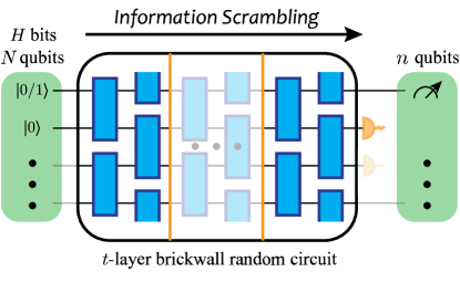
FIG. 1: Quantum channel scenery for probing information scrambling dynamics. One encodes $H$-bits of information into $H$ arbitrarily chosen qubits of an $N$-qubit system. Then after $t$ layers of “brick wall”-structured random circuits, we retrieve information from a randomly selected $n$-qubit subsystem. Every “brick” (blue rectangle) represents a random unitary gate between two adjacent qubits.

To study the scrambling dynamics of quantum systems directly from the quantum information perspective, we consider Holevo information, which, by definition, describes the information encoded in an ensemble of quantum states [31]. Since the Holevo information is preserved under unitary evolution, it can distinguish between the ideal case and the decoherence and thus allows us to verify information scrambling in noisy quantum systems [32, 15, 33]. Based on Holevo information, progress has been made in understanding the distinguishability of black hole microstates in black hole theory [34, 35, 36]. However, these works only focus on the final states of the black holes after fast scrambling, while the dynamics toward scrambling is not considered. Another related method is to apply an operator-state mapping and study the mutual information [32, 21, 37] or the tripartite information [21] between the input system and the output system.

Here, we consider the Hovelo information under random unitary circuits in a qubit system and show phase-transition-like behavior in the retrieved information. For long enough circuits, as the size of the subsystem increases across a threshold of one half, the retrieved information increases non-analytically from zero to finite values, and further increases until saturation at another transition point. This phenomenon is observed from numerical simulation, and is also confirmed by analytical derivation. We examine the scrambling dynamics through the convergence of the average Holevo information toward its infinite-time limit as the circuit depth grows. We also study the critical behavior near the phase transition points. As the Hovelo information only measures the retrieved classical information from a quantum system, finally we use coherent information to quantify scrambling of quantum information in the same system and find similar phase-transition-like behavior for the coherent information.

II Information Scrambling in Random Quantum Circuits

Consider an $N$-qubit quantum system. As shown in Fig. 1, we store $H$ bits of classical information by randomly selecting a subsystem of $H$ qubits and preparing them into an ensemble of pure states $\left\{p_{i},|\psi_{i}^{\mathrm{init}}\rangle\right\}$ with $p_{i}=\frac{1}{2^{H}}$ and ${|\psi_{i}^{\mathrm{init}}\rangle}$ be the $2^{H}$ orthogonal states in computational basis. The system then evolves under a randomly generated Clifford circuit $U$, after which one part of it $\mathcal{E}$ is regarded as the environment and traced out. For the remaining system $Q$ containing $n$ qubits, we can denote the amount of classical information that can be retrieved as $\chi_{Q}$, which is given by the Holevo information

$$\chi_{Q}\left(\left\{|\psi_{i}^{\mathrm{init}}\rangle\right\},U\right)=S\left(\sum_{i}p_{i}\rho_{i}^{Q}\right)-\sum_{i}p_{i}S\left(\rho_{i}^{Q}\right),$$ (1)

where $\rho_{i}^{Q}=\mathrm{Tr}_{\mathcal{E}}(U|\psi_{i}^{\mathrm{init}}\rangle\langle\psi_{i}^{\mathrm{init}}|U^{\dagger})$ is the output density matrix of the system $Q$, and $S$ is the von Neumann entropy.

We adopt the periodic boundary condition for the qubits and consider random circuits of the “brick wall” configuration, as shown in Fig. 1. The circuit comprises $t$ layers of alternatingly layered bricks in which each brick represents a uniformly sampled two-qubit random Clifford gate. We denote $\mathcal{U}_{t}$ as the set of all possible unitaries constructed in this way with $t$ layers. Note that we choose the Clifford circuit mainly because of the convenience in numerical simulation [38, 39]. Also, we specify the set of input quantum states $\left\{|\psi_{i}^{\mathrm{init}}\rangle\right\}=\left\{|\gamma_{1}\gamma_{2}...\gamma_{H}\rangle_{Q_{H}}|0...0\rangle_{\text{others}}\right\}_{\gamma_{i}\in\{0,1\}}$ where $Q_{H}$ is a randomly selected subsystem with $H$ qubits. We can thus write the Holevo information as $\chi_{Q}\left(\left\{|\psi_{i}^{\mathrm{init}}\rangle\right\},U\right)\equiv\chi_{Q,Q_{H}}\left(U\right)$. Note that the choices of $Q$ and $Q_{H}$ are arbitrary and does not need to have any specific spatial pattern.

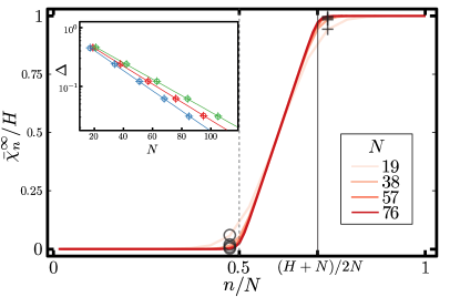
FIG. 2: Average Holevo information $\bar{\chi}_{n}^{\infty}$ of an $n$-qubit subsystem $Q$ in the steady state. For the later convenience to examine the behavior near the phase transition point, we choose $N$ to be multiples of $19$. For different $N$ we fix its ratio with the encoded classical information as $N:H=19:8$. The curve becomes sharper around the two phase transition points as $N$ increases. Note that the behavior is similar for generic $1\leq H\leq N$. The inset shows the result of finite-size scaling. We focus on the difference $\Delta$ between $\bar{\chi}_{n}^{\infty}$ and the thermodynamic limit $\chi_{n}^{\text{thermal}}$ when $n$ is chosen to be close to the phase transition point $\frac{n}{N}=\frac{1}{2}$ (circle) and $\frac{n}{N}=\frac{H+N}{2N}$ (cross). Specifically, for $n$ smaller than $\frac{N}{2}$ we calculate $\Delta_{1}=\bar{\chi}_{n}^{\infty}$, and for $n$ larger than $\frac{N+H}{2}$ we calculate $\Delta_{2}=H-\bar{\chi}_{n}^{\infty}$. The blue, red, and green lines are for three different ratios of $N:H=17:6,\allowbreak 19:8,\allowbreak 21:10$, respectively. When $n,N,H$ increase under a fixed ratio, $\Delta_{1}$ and $\Delta_{2}$ decay exponentially. For each data point, we sample $10^{6}$ times. The long-time limit is approximated by choosing $t=3N$ as described in the main text.

After obtaining the Holevo information contained in a randomly selected subsystem from the above setting, we further average over all possible subsystem $Q$, all possible input states, and all the circuits with the same depth $t$ to get

$$\bar{\chi}_{n}^{t}=\frac{1}{|\mathcal{U}_{t}|}\frac{1}{|\mathcal{S}_{n}|}\frac{1}{|\mathcal{S}_{H}|}\sum_{U\in\mathcal{U}_{t}}\sum_{Q\in\mathcal{S}_{n}}\sum_{Q_{H}\in\mathcal{S}_{H}}\chi_{Q,Q_{H}}\left(U\right),$$ (2)

where $\mathcal{S}_{k}$ denotes the set of all subsystems with $k$ qubits.

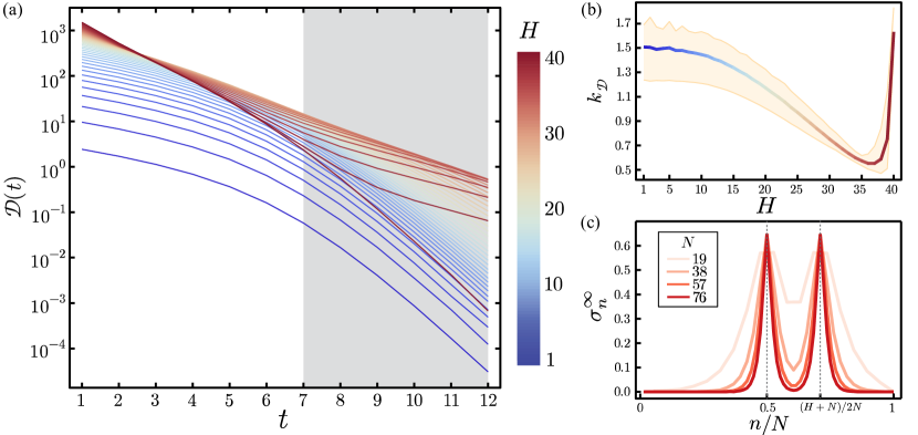
FIG. 3: (a) Distance $\mathcal{D}(t)$ of the averaged Holevo information from its long time limit. We calculate for $N=40$ and $H$ from $1$ (blue) to $N$ (red). Each data point is obtained by averaging over $10^{6}$ random circuits and initial states. (b) The decay rate of $\mathcal{D}(t)$ in the greyed region of (a), defined as $k_{\mathcal{D}}^{7,12}$ in the main text. The shaded region around the curve shows the confidence interval whose upper and lower bounds are estimated by the maximum and minimum slopes in the greyed region in (a). (c) Standard deviation $\sigma_{n}^{\infty}$ of Holevo information $\chi_{Q}(U)$ in $n$ qubit subsystem $Q\in\mathcal{S}_{n}$. The steady-state is approximated by setting circuit depth $t=3N$. We fix the ratio $N:H=19:8$. At the two phase transition points $\frac{n}{N}=\frac{1}{2},\frac{H+N}{2N}$, the peaks become sharper as $N$ grows.

As shown in Fig. 2, we numerically compute the long time limit of the Holevo information $\bar{\chi}_{n}^{\infty}=\lim_{t\rightarrow\infty}\bar{\chi}_{n}^{t}$ by setting $t=3N$. Theoretically, $\Omega(N)$ layers are needed for the initially localized information to propagate over the whole system [7, 40, 41], and here, we verify the convergence of Holevo information by comparing the results at $t=3N$ with those at $t=4N$. A phase-transition-like behavior can be observed: For small system size $n$, we are not able to retrieve any information; When $n$ reaches half of the system size, information starts emerging at a constant rate of two bits of classical information per qubit; Finally, the retrievable information reaches its maximum value through another sharp nonanalytical change, indicating that all of the initially encoded information can be reliably recovered. We perform finite-size scaling near the two points to further analyze the phase-transition-like behavior. As shown in the inset of Fig. 2, by fixing a ratio at $\frac{n}{N}<\frac{1}{2}$ and $\frac{n}{N}>\frac{H+N}{2N}$, respectively, and increasing $n,N,H$ simultaneously, $\bar{\chi}_{n}^{\infty}$ converges exponentially towards its thermodynamic limit. Note that one can get the same value of $\bar{\chi}_{n}^{\infty}$ without averaging over the choice of $Q_{H}$. This can be understood from the definition of scrambling and from the symmetry of the random unitary group [28].

Indeed, if the circuit is sampled uniformly over the $N$-qubit Clifford group, we can calculate theoretically the average Holevo information $\bar{\chi}_{n}^{\infty}$ for arbitrary $n,N,H$, and it agrees well with the numerical result obtained above for layered random two-qubit Clifford gates. For more details, see Appendix LABEL:Asec. Specifically, if we take the thermodynamic limit $n,N,H\rightarrow\infty$ with the ratio $\frac{n}{N}\equiv r_{n},\frac{H}{N}\equiv r_{H}$ held constant, this theoretical value $\bar{\chi}_{n}^{\infty}$ converges to

$$\frac{1}{H}\chi_{n}^{\text{thermal}} =\begin{cases}0&r_{n}\leq\frac{1}{2}\\ (2r_{n}-1)/r_{H}&\frac{1}{2}<r_{n}\leq\frac{1}{2}(1+r_{H})\\ 1&r_{n}>\frac{1}{2}(1+r_{H})\end{cases}.$$ (3)

This further allows us to define the critical exponent

$$k\equiv\lim_{\tau\rightarrow 0^{+}}\frac{\log\left|f(\tau)\right|}{\log\left|\tau\right|}=1$$ (4)

where for the first transition point $\tau=r_{n}-\frac{1}{2}$, $f(\tau)=\frac{1}{H}\chi_{n}^{\text{thermal}}$ and similarly for the second transition point.

III Information Scrambling Dynamics

From the evolution of the Holevo information, we can study the information scrambling dynamics of quantum systems. For example, here we study how the long-time limit of the average Holevo information is approached. We compare the average Holevo information for different subsystem sizes $\left\{\bar{\chi}_{n}^{t}\right\}_{n=1}^{N}$ with its long-time limit. We use 2-norm to measure their difference

$$\mathcal{D}(t)=\sum_{n=1}^{N}(\bar{\chi}_{n}^{t}-\bar{\chi}_{n}^{\infty})^{2}.$$ (5)

From the numerical simulation, we plot $\mathcal{D}(t)$ for the system size $N=40$ and $H$ ranging from $1$ to $N$, as shown in Fig. 3a. We observe that $\left\{\bar{\chi}_{n}^{t}\right\}_{n=1}^{N}$ converges under time evolution roughly exponentially. Further, the decaying rate, which corresponds to the scrambling speed, varies for different initial Holevo information $H$.

To compare the speed of scrambling between $1\leq H\leq N$, we extract the average slope on the semi-log plot of $\mathcal{D}(t)$ between time $t$ and $t^{\prime}$ as

$$k_{\mathcal{D}}^{t,t^{\prime}}=\left|\frac{\log\mathcal{D}(t)-\log\mathcal{D}(t^{\prime})}{t-t^{\prime}}\right|$$ (6)

as shown in Fig. 3b. The upper and lower confidence bounds are roughly estimated by the maximum and minimum slope in the region. For the same set of circuits, the scrambling rate slows down when an increasing amount of information is encoded into the system until close to $\frac{H}{N}\sim 1$ where the tendency reverses, which may be caused by the finite size effect.

We further study the information scrambling behavior of individual realizations $U$ of random circuits by comparing the Holevo information distribution $\chi_{Q,Q_{H}}\left(U\right)$ with the average value over different realizations. We characterize it by the standard deviation $\sigma_{n}^{t}$

$$\left(\sigma_{n}^{t}\right)^{2}=\frac{1}{|\mathcal{U}_{t}|}\frac{1}{|\mathcal{S}_{n}|}\frac{1}{|\mathcal{S}_{H}|}\sum_{U\in\mathcal{U}_{t}}\sum_{Q\in\mathcal{S}_{n}}\sum_{Q_{H}\in\mathcal{S}_{H}}(\chi_{Q,Q_{H}}\left(U\right)-\bar{\chi}_{n})^{2}.$$ (7)

As shown in Fig. 3c, we numerically compute its long time limit $\sigma_{n}^{\infty}=\lim_{t\rightarrow\infty}\sigma_{n}^{t}$ by setting $t=3N$. The ratio $N:H=19:8$ is set in accordance with Fig. 2. As we can see, $\sigma_{n}^{\infty}$ is asymptotically zero not only in the region $\frac{n}{N}<\frac{1}{2}$ and $\frac{n}{N}>\frac{N+H}{2N}$, where $\bar{\chi}_{n}^{\infty}$ already saturates, but also in the region $\frac{1}{2}<\frac{n}{N}<\frac{N+H}{2N}$. This suggests that information almost fully scrambles even for a single typical random circuit. Only at the two phase transition points can we get finite standard deviations, which do not increase with $N$, $H$ and $n$ so the relative fluctuation is decreasing for larger systems.

IV Similar Phase-Transition-Like Behavior for Coherent Information

After studying the information scrambling dynamics by the classical information, a natural next step is to consider if the same scrambling dynamics can be probed by quantum information as well, particularly if the same phase-transition-like behavior persists.

Coherent information [42, 43, 44] quantifies the remaining quantum information after a state goes through a quantum channel, with similar properties as the mutual information in classical communication. The coherent information is also related to the reversibility of the quantum channel [45] and the condition of quantum error correction [42], thus lies at the heart of understanding the difference between classical and quantum information communication.

As shown in the inset of Fig. 4, similar to the model for Holevo information, we encode quantum information of $C$ in $N$ qubits with periodic boundary conditions, apply random Clifford circuit $U\in\mathcal{U}_{t}$ and regard a randomly selected subsystem $\mathcal{E}$ as the environment to be traced off. The difference is that the system’s initial state $Q^{\text{init}}$ would be an ensemble $\rho^{\mathrm{init}}=\frac{1}{2^{C}}I_{Q_{C}}\otimes|0...0\rangle\langle 0...0|_{\text{others}}$, where $Q_{C}$ represents a subsystem of randomly selected $C$ qubits. This ensemble can be seen as a mixture of $\left\{|\psi_{i}^{\mathrm{init}}\rangle\right\}$ with equal probabilities. We write the final state of the $n$-qubit system $Q$ as $\rho^{Q}$. The circuit, together with tracing out the environment $\mathcal{E}$, forms a quantum channel $\mathcal{C}$. The coherent information can thus be calculated as [42, 43, 44]

$$\eta_{Q}(\rho^{\mathrm{init}},\mathcal{C})=S(\rho^{Q})-S(\rho,\mathcal{C}),$$ (8)

where $S(\rho,\mathcal{C})$ is the entropy exchange. By definition, to calculate $S(\rho,\mathcal{C})$, we need to purify $Q^{\text{init}}$ using a reference system $R^{\text{init}}$ before applying the quantum channel. Then we get $S(\rho,\mathcal{C})=S(\rho^{QR})$.

Similar to what we have done for Holevo information, we write $\eta_{Q}(\rho^{\mathrm{init}},\mathcal{C})\equiv\eta_{Q,Q_{H}}(\mathcal{C})$ and average over the system $Q$, the input states and the circuit to get

$$\bar{\eta}_{n}^{t}=\frac{1}{|\mathcal{U}_{t}|}\frac{1}{|\mathcal{S}_{n}|}\frac{1}{|\mathcal{S}_{C}|}\sum_{U\in\mathcal{U}_{t}}\sum_{Q\in\mathcal{S}_{n}}\sum_{Q_{H}\in\mathcal{S}_{C}}\eta_{Q,Q_{H}}(\mathcal{C}).$$ (9)

Finally, the long-time limit $\bar{\eta}_{n}^{\infty}$ is approximated by $t=3N$.

The results for various system sizes are shown in Fig. 4 which has a phase-transition-like behavior similar to that of the Holevo information, although the phase transition points are at $\frac{n}{N}=\frac{N-C}{2N},\frac{n}{N}=\frac{N+C}{2N}$. To see how these transition points correspond to those for the Holevo information, note that the second transition point $\frac{n}{N}=\frac{N+C}{2N}$ is the same for both cases. On the other hand, when $\frac{n}{N}<\frac{N-C}{2N}$, all the information goes into the environment, making the coherent information saturate to its lower bound $\frac{\bar{\eta}_{n}^{\infty}}{C}=-1$. The phase transition point at $\frac{n}{N}=\frac{N-C}{2N}$ thus corresponds to that of the Holevo information in the environment $\mathcal{E}$ rather than in the system $Q$. Finally, when $n<\frac{N}{2}$ we have negative $\bar{\eta}_{n}^{\infty}$, indicating that no quantum information can be retrieved from the output system. This is in agreement with the result for Holevo information.

FIG. 4: Average coherent information $\bar{\eta}_{n}^{\infty}$ of an $n$-qubit subsystem $Q$ in the steady state. Like the settings for the Holevo information, we scale the system size $N$ and the total encoded quantum information $C$ by $N:C=19:8$. As $N$ grows, the curve shows two phase transition points at $\frac{n}{N}=\frac{N-C}{2N},\allowbreak\frac{n}{N}=\frac{N+C}{2N}$, respectively. The inset shows an illustration of the numerical scheme. The initial state, encoded as an ensemble into $Q^{\text{init}}$, is purified by $R^{\text{init}}$. After a random circuit $U\in\mathcal{U}_{t}$, part of the system $\mathcal{E}$ is traced out as the environment. Together they form a quantum channel $\mathcal{C}$. The coherent information encoded in the system $Q$ can thus be computed with the help of the reference system $R$.

V Discussions

In summary, in this work we use the spatial distribution of Holevo information to characterize the information scrambling process. The information converges to zero in the thermodynamic limit when we consider subsystem sizes smaller than half the system. When exceeding this threshold, the extractable classical information increases by two bit per added qubit until its saturation to the total encoded information. This can serve as a scrambling criterion, and its comparison with others, including Haar scrambled [7] and Page scrambled [6] criteria, is of great interest. We study how the system approaches the long-time limit and how the convergence speed varies with the amount of encoded information. We also find that variation around the average behavior is vanishingly small almost everywhere apart from the two phase transition points, which implies that in the thermodynamic limit, almost all random circuits would meet the scrambling criteria. Finally, we find that the coherent information possesses a similar phase-transition-like behavior.

One can regard the discarded environment in our model as the qubit loss error from the quantum error correction (QEC) perspective [46, 47]. Thus the phase transition point $\frac{n}{N}=\frac{N+C}{2N}$ of coherent information would correspond to the condition of perfect decoding. Specifically, our model uses the random circuit to encode $C$ logical qubits in $N$ physical qubits. This code can tolerate the loss of $\frac{N-C}{2}$ located qubits which saturates the quantum Singleton bound [48].

Although here we restrict the calculation to Clifford gates for numerical convenience, this method using Holevo information to characterize information scrambling should largely be applicable to generic quantum systems. Specifically, this process of encoding information by a set of initial states and calculating the Holevo information of a selected subsystem in the final states does not require any special property of the intermediate quantum dynamics. We can thus easily extend the unitary evolution to arbitrary quantum channels, although the detailed late time physics may depend on specific models and remains an open direction for future research. Therefore it may provide a universal tool for probing quantum information scrambling dynamics.

APPENDIX A PROOF OF EQ. (LABEL:EQ:THERMAL)

1 Model Description

Consider an $n$-qubit subsystem $Q$ in an $N$-qubit Clifford system. In the main text, we have already specified that the intitial quantum states are $\left\{|\psi_{i}^{\mathrm{init}}\rangle\right\}=\left\{|\gamma_{1}\gamma_{2}...\gamma_{H}\rangle_{Q_{H}}|0...0\rangle_{\text{others}}\right\}_{\gamma_{i}\in\{0,1\}}$ each appearing with equal probability $\frac{1}{2^{H}}$. After a random Clifford circuit $U$, we denote the final state as $|\psi_{i}\rangle$. The Holevo Information can be written as $\chi_{n}=S_{n}(U\frac{1}{2^{H}}\sum_{2^{H}}|\psi_{i}\rangle\langle\psi_{i}|U^{\dagger})-\frac{1}{2^{H}}\sum_{2^{H}}S_{n}(U|\psi_{i}\rangle\langle\psi_{i}|U^{\dagger})$, where $S_{n}(\rho)$ represents the entropy of the $n$-qubit subsystem $Q$.

When we average it over all possible circuits with its depth large enough, the first and the second term converges respectively. Thus, we can decompose it into two parts:

$$\bar{\chi}_{n}=\mathbb{E}S_{n,H}-\mathbb{E}S_{n,0}$$ (10)

where we write $\rho_{h}=\frac{1}{2^{h}}\sum_{2^{h}}|\psi_{i}\rangle\langle\psi_{i}|$ and $S_{n,h}=S_{n}(U\rho_{h}U^{\dagger})$ for convenience.

The Clifford unitary with large depth will bring any initial state $\rho_{h}$ into a finite set $\mathrm{Orb}(\rho_{h},\mathcal{U}^{N})$ with uniform probability distribution, where $\mathrm{Orb}(\rho_{h},\mathcal{U}^{N})$ is the orbit of $\rho_{h}$ under the $N$-qubit Clifford group $\mathcal{U}^{N}$. Thus the probability $\text{Prob}(S_{n,h}=x)$ would be proportional to the number of states $\rho\in\mathrm{Orb}(\rho_{h})$ that satisfies $S_{n}(\rho)=x$. Here we calculate the number of elements in such set $\left|\left\{\rho\in\mathrm{Orb}(\rho_{h},\mathcal{U}^{N})|S_{n}(\rho)=x\right\}\right|$ and give the expectation value $\mathbb{E}S_{n,h}$.

2 Outline of the Proof

Any state $\rho_{h}$ that satisfies $S(\rho_{h})=x$ can be transformed by a local Clifford unitary $U\in G=\left\{U(n)\otimes U(m)\right\}$ to $\rho_{h}^{x}$ which we write under the stabilizer formalism [39, 38]

$$\begin{bmatrix}[cccc|cccc]X&&&&X&\\ Z&&&&Z&\\ &Z&&&&Z\\ &&Z&&&&Z\\ &&&Z&\\ &&&&&&&Z\end{bmatrix}\BMAT(@)[1pt,10pt,0pt]{l}{cccc}\scalebox{0.7}[0.5]{\rotatebox{90.0}{{\hbox{\underbrace{\hskip 43.1997pt}}}}}\raisebox{10.79993pt}{$\scriptstyle\;k_{1}\text{ pairs}$}\\ \scalebox{0.7}[0.5]{\rotatebox{90.0}{{\hbox{\underbrace{\hskip 43.1997pt}}}}}\raisebox{10.79993pt}{$\scriptstyle\;k_{2}$}\\ \scalebox{0.7}[0.5]{\rotatebox{90.0}{{\hbox{\underbrace{\hskip 21.59985pt}}}}}\raisebox{5.39996pt}{$\scriptstyle\;l_{1}$}\\ \scalebox{0.7}[0.5]{\rotatebox{90.0}{{\hbox{\underbrace{\hskip 21.59985pt}}}}}\raisebox{5.39996pt}{$\scriptstyle\;l_{2}$}\\$$ (11)

where $n+m=N$, $x=n-l_{1}$ and the number of stabilizer operators

$$2k_{1}+k_{2}+l_{1}+l_{2}=n+m-h$$ (12)

We can constraint the four parameters by

$$\left\{\begin{aligned} k_{1}+k_{2}+l_{1}&\leq n\\ k_{1}+k_{2}+l_{2}&\leq m\\ k_{1},k_{2},l_{1},l_{2}&\geq 0\end{aligned}\right.$$ (13)

We can further simplify our question by

$$\left\{\rho\in\mathrm{Orb}(\rho_{h},\mathcal{U}^{N})|S_{n}(\rho)=x\right\}=\left\{\rho\in\mathrm{Orb}(\rho_{h},G)|S_{n}(\rho)=x\right\}=\left\{\rho\in\mathrm{Orb}(\rho_{h}^{x},G)\right\}$$ (14)

This can be given by directly using the common state Eq. 11 that all the states with the same entropy can reach by local unitaries.

With the help of Lagrange’s orbit-stabilizer theorem $\left|\mathrm{Orb}(\rho_{h}^{x},G)\right|=\frac{\left|G\right|}{\left|\mathrm{Stab}(\rho_{h}^{x},G)\right|}$, we only need

• the order of unitary group $\left|G\right|$

• the order of stabilizer $\left|\mathrm{Stab}(\rho_{h}^{x},G)\right|$. Here the stabilizer $\mathrm{Stab}(\rho_{h}^{x},G)$ represents the set of elements in $G$ that makes $\rho_{h}^{x}$ invariant.

We can get $\left|G\right|$ directly from the volume of $N$ qubit Clifford group $Cl(N)=\prod_{j=1}^{N}2(4^{j}-1)4^{j}$ [49]

$$\left|G\right|=Cl(n)\times Cl(m)$$ (15)

Based on basic combinatorics, we have from Sec. A. 3

$$\left|\mathrm{Stab}(\rho_{h}^{x},G)\right|= \left(\prod_{j=1}^{k_{1}}\left(4^{j}-1\right)4^{j}2\right)2^{2k_{1}(k_{2}+l_{1})}2^{2k_{1}l_{2}}$$ (16)

$$\times 2^{k_{2}}2^{2k_{2}}2^{\frac{1}{2}k_{2}(k_{2}+2l_{1}+1)}2^{\frac{1}{2}k_{2}(k_{2}+2l_{2}+1)}4^{h_{1}k_{2}}4^{h_{2}k_{2}}\left(\prod_{j=0}^{k_{2}-1}\left(2^{k_{2}}-2^{j}\right)\right)2^{l_{1}k_{2}}2^{l_{2}k_{2}}$$

$$\times 2^{l_{1}+\frac{1}{2}l_{1}(l_{1}+1)}\left(\prod_{j=0}^{l_{1}-1}\left(2^{l_{1}}-2^{j}\right)\right)4^{h_{1}l_{1}}$$

$$\times 2^{l_{2}+\frac{1}{2}l_{2}(l_{2}+1)}\left(\prod_{j=0}^{l_{2}-1}\left(2^{l_{2}}-2^{j}\right)\right)4^{h_{2}l_{2}}$$

$$\times Cl(h_{1})Cl(h_{2})$$

where

$$h_{1} =n-k_{1}-k_{2}-l_{1}$$

$$h_{2} =m-k_{1}-k_{2}-l_{2}$$

When $n,h,N$ is fixed, the order of the orbit can be determined by the four parameters $k_{1},k_{2},l_{1},l_{2}$.

$$\left|\mathrm{Orb}(\rho_{h}^{x},G)\right|=\frac{\left|G\right|}{\left|\mathrm{Stab}(\rho_{h}^{x},G)\right|}\equiv t_{k_{1},k_{2},l_{1},l_{2}}$$ (17)

Recall that $x=n-l_{1}$, we have

$$\mathbb{E}S_{n,h}=\frac{\sum(n-l_{1})\times t_{k_{1},k_{2},l_{1},l_{2}}}{\sum t_{k_{1},k_{2},l_{1},l_{2}}}$$ (18)

where the sum is over all possible $k_{1},k_{2},l_{1},l_{2}$ under the constraint Eq. (13).

By setting $h=0$ and $h=H$, this gives both the terms in Eq. (10). For specific values of $n,H,N$, the calculation agrees well with our numerical result in the main text, as shown in Fig. 5

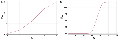
FIG. 5: Numerical simulation using Monte Carlo method (red) and analytic calculation (blue) of Holevo information $\bar{\chi}_{n}$. (a) $N=5$ and $H=3$. (b) $N=30$ and $H=15$. The two lines almost completely overlap.

To further prove Eq. (3) in the main text, we first observe that $t_{k_{1},k_{2},l_{1},l_{2}}$ is varying in an exponential way for different $k_{1},k_{2},l_{1},l_{2}$. When $n,N,H$ is large, the expected value of $n-l_{1}$ would correspond to $k_{1},k_{2},l_{1},l_{2}$ where $t_{k_{1},k_{2},l_{1},l_{2}}$ reaches maximum.

Assuming $k_{1},k_{2},l_{1},l_{2}\rightarrow\infty$ and ignoring constant terms, we can convert the question of where $\log_{2}t_{k_{1},k_{2},l_{1},l_{2}}$ reaches maximum to be where $f(k_{1},k_{2},l_{1},l_{2})$ reaches maximum, here

$$-f(k_{1},k_{2},l_{1},l_{2}) =2k_{1}(N-H-k_{1})+3k_{1}$$

$$+3k_{2}+2k_{2}(k_{2}+l_{1}+l_{2}+H)$$

$$+l_{1}\left(\frac{3}{2}l_{1}+\frac{1}{2}\right)+l_{2}\left(\frac{3}{2}l_{2}+\frac{1}{2}\right)$$

$$+2(n-k_{1}-k_{2}-l_{1})(n-k_{1}-k_{2}+1)$$

$$+2(N-n-k_{1}-k_{2}-l_{2})(N-n-k_{1}-k_{2}+1)$$

Combining with the constraints in Eq. (12) and Eq. (13), $f(k_{1},k_{2},l_{1},l_{2})$ reaches maximum when

$$\begin{array}[]{c}n<\frac{N-h}{2}\\ \\ \left\{\begin{aligned} k_{1}&=n\\ k_{2}&=0\\ l_{1}&=0\\ l_{2}&=N-h-2n\end{aligned}\right.\end{array}\begin{array}[]{c}\frac{N-h}{2}\leq n\leq\frac{N+h}{2}\\ \\ \left\{\begin{aligned} k_{1}&=(N-h)/2\\ k_{2}&=0\\ l_{1}&=0\\ l_{2}&=0\end{aligned}\right.\end{array}\begin{array}[]{c}n>\frac{N+h}{2}\\ \\ \left\{\begin{aligned} k_{1}&=N-n\\ k_{2}&=0\\ l_{1}&=2n-N-h\\ l_{2}&=0\end{aligned}\right.\end{array}$$ (19)

the proof is given in Sec. A. 4

By Eq. (18) we get

$$\mathbb{E}S_{n,h}=\min(n,N+h-n)$$ (20)

Finally the Holevo information

$$\bar{\chi}_{n}=\mathbb{E}S_{n,H}-\mathbb{E}S_{n,0}=\begin{cases}0&n<\frac{N}{2}\\ 2n&\frac{N-H}{2}\leq n\leq\frac{N+H}{2}\\ H&n>\frac{N+H}{2}\end{cases}$$ (21)

3 Proof of Eq. (16)

We count the number of elements in $G$ that makes $\rho_{h}^{x}$ invariant. Every non-trivial elements in the $G=\left\{U(n)\otimes U(m)\right\}$ maps the set of stabilizer operators in Eq. 11 to a new one. We count how many of the resulting stabilizer operators form a equivalent state to the original. Two sets of stabilizers are equivalent if they are the same under standard stabilizer multiplication operations.

Below we split Eq. (16) into factors and explain them respectively.

• $\left(\prod_{j=1}^{k_{1}}\left(4^{j}-1\right)4^{j}2\right)2^{2k_{1}(k_{2}+l_{1})}2^{2k_{1}l_{2}}$. For the first $2k_{1}$ stabilizers, the two in each pair do not commute with each other in two subsystems. This property would preserve for arbitrary local transformation.

• $2^{k_{2}}2^{2k_{2}}2^{\frac{1}{2}k_{2}(k_{2}+2l_{1}+1)}2^{\frac{1}{2}k_{2}(k_{2}+2l_{2}+1)}4^{h_{1}k_{2}}4^{h_{2}k_{2}}\left(\prod_{j=0}^{k_{2}-1}\left(2^{k_{2}}-2^{j}\right)\right)2^{l_{1}k_{2}}2^{l_{2}k_{2}}$. For the next $k_{2}$ stabilizers, the combination of arbitrary elements in $l_{1}+l_{2}$ stabilizers are reachable by $G$.

• $2^{l_{1}+\frac{1}{2}l_{1}(l_{1}+1)}\left(\prod_{j=0}^{l_{1}-1}\left(2^{l_{1}}-2^{j}\right)\right)4^{h_{1}l_{1}}$. The local unitaries in $G$ can only bring $l_{1}$ stabilizers which is local in $Q$ to another local stabilizer in $Q$.

• $2^{l_{2}+\frac{1}{2}l_{2}(l_{2}+1)}\left(\prod_{j=0}^{l_{2}-1}\left(2^{l_{2}}-2^{j}\right)\right)4^{h_{2}l_{2}}$. The same as $l_{1}$

• $Cl(h_{1})$. After determining all the stabilizers above, there still exists $h_{1}$ degrees of freedom in $Q$. This corresponds to $Cl(h_{1})$ elements.

• $Cl(h_{2})$. The same as $h_{1}$.

4 Proof of Eq. (19)

$f(k_{1},k_{2},l_{1},N-h-(2k_{1}+k_{2}+l_{1}))$ is a concave function for $k_{1},k_{2},l_{1}$. This can be seen from its Hessian matrix $\left(\begin{array}[]{ccc}-8&-4&-6\\ -4&-7&-3\\ -6&-3&-6\end{array}\right)$

At Eq. (19), we only need to prove that $f$ achieves its local maximum to prove that it also achieves global maximum over the convex region defined in Eq. (13). Further, we observe that the condition in Eq. (19) coincides with the boundaries of the region. To verify them as local maximum, we can compare the gradient $\nabla f=\left(\begin{array}[]{c}\partial_{k_{1}}f\\ \partial_{k_{2}}f\\ \partial_{l_{1}}f\end{array}\right)=\left(\begin{array}[]{c}-2(1+h+4k_{1}+2k_{2}+3l_{1}-N-2n)\\ -(1/2)-h-4k_{1}-7k_{2}-3l_{1}+N+2n\\ -3h-6k_{1}-3k_{2}-6l_{1}+N+4n\end{array}\right)$ with the orientation of boundaries $g_{i}\leq 0$. Specifically, we solve

$$\nabla(f-\sum_{i}\mu_{i}g_{i})=0$$ (22)

and verify $\mu_{i}\geq 0\quad\forall i$.

When $n<\frac{N-h}{2}$, the constraints are $\left\{\begin{array}[]{c}g_{1}=k_{1}+k_{2}+l_{1}-n\\ g_{2}=-k_{2}\\ g_{3}=-l_{1}\end{array}\right.$. Solving Eq. (22) we get

$$\bm{\mu}=\left(\begin{array}[]{c}2(N-h-2n-1)\\ N-h-2n-(3/2)\\ N+h-2n-2\end{array}\right)$$ (23)

When $\frac{N-h}{2}<n<\frac{N+h}{2}$, the constraints are $\left\{\begin{array}[]{c}g_{1}=2k_{1}+k_{2}+l_{1}-(N-h)\\ g_{2}=-k_{2}\\ g_{3}=-l_{1}\end{array}\right.$ where $g_{1}$ comes from $l_{2}\geq 0$. Solving Eq. (22) we get

$$\bm{\mu}=\left(\begin{array}[]{c}2n+h-N-1\\ -1/2\\ N+h-2n-1\end{array}\right)$$ (24)

When $n>\frac{N+h}{2}$, the constraints are $\left\{\begin{array}[]{c}g_{1}=2k_{1}+k_{2}+l_{1}-(N-h)\\ g_{2}=-k_{2}\\ g_{3}=-k_{1}-l_{1}+n-h\end{array}\right.$ where $g_{3}$ comes from $k_{1}+k_{2}+l_{2}\leq m$. Solving Eq. (22) we get

$$\bm{\mu}=\left(\begin{array}[]{c}-2+h+2n-N\\ -(3/2)-h+2n-N\\ -2(1+h-2n+N)\end{array}\right)$$ (25)

All of $\mu_{i}$ above are non-negative.

References

- Larkin and Ovchinnikov [1969] A. Larkin and Y. N. Ovchinnikov, Quasiclassical method in the theory of superconductivity, Sov Phys JETP 28, 1200 (1969).
- Berry [1989] M. Berry, Quantum chaology, not quantum chaos, Phys. Scr. 40, 335 (1989).
- Maldacena et al. [2016] J. Maldacena, S. H. Shenker, and D. Stanford, A bound on chaos, J. High Energ. Phys. 2016 (8), 106.
- Rozenbaum et al. [2017] E. B. Rozenbaum, S. Ganeshan, and V. Galitski, Lyapunov Exponent and Out-of-Time-Ordered Correlator’s Growth Rate in a Chaotic System, Phys. Rev. Lett. 118, 086801 (2017).
- Roberts and Yoshida [2017] D. A. Roberts and B. Yoshida, Chaos and complexity by design, J. High Energ. Phys. 2017 (4), 121.
- Sekino and Susskind [2008] Y. Sekino and L. Susskind, Fast scramblers, J. High Energy Phys. 2008 (10), 065.
- Hayden and Preskill [2007] P. Hayden and J. Preskill, Black holes as mirrors: Quantum information in random subsystems, J. High Energy Phys. 2007 (9).
- Shenker and Stanford [2014] S. H. Shenker and D. Stanford, Black holes and the butterfly effect, J. High Energ. Phys. 2014 (3), 67.
- Bañuls et al. [2017] M. C. Bañuls, N. Y. Yao, S. Choi, M. D. Lukin, and J. I. Cirac, Dynamics of quantum information in many-body localized systems, Phys. Rev. B 96, 1 (2017).
- Swingle [2018] B. Swingle, Unscrambling the physics of out-of-time-order correlators, Nature Phys 14, 988 (2018).
- Zhang et al. [2017] J. Zhang, G. Pagano, P. W. Hess, A. Kyprianidis, P. Becker, H. Kaplan, A. V. Gorshkov, Z.-X. Gong, and C. Monroe, Observation of a many-body dynamical phase transition with a 53-qubit quantum simulator, Nature 551, 601 (2017).
- Arute et al. [2019] F. Arute, K. Arya, R. Babbush, D. Bacon, J. C. Bardin, R. Barends, R. Biswas, S. Boixo, F. G. Brandao, D. A. Buell, B. Burkett, Y. Chen, Z. Chen, B. Chiaro, R. Collins, W. Courtney, A. Dunsworth, E. Farhi, B. Foxen, A. Fowler, C. Gidney, M. Giustina, R. Graff, K. Guerin, S. Habegger, M. P. Harrigan, M. J. Hartmann, A. Ho, M. Hoffmann, T. Huang, T. S. Humble, S. V. Isakov, E. Jeffrey, Z. Jiang, D. Kafri, K. Kechedzhi, J. Kelly, P. V. Klimov, S. Knysh, A. Korotkov, F. Kostritsa, D. Landhuis, M. Lindmark, E. Lucero, D. Lyakh, S. Mandrà, J. R. McClean, M. McEwen, A. Megrant, X. Mi, K. Michielsen, M. Mohseni, J. Mutus, O. Naaman, M. Neeley, C. Neill, M. Y. Niu, E. Ostby, A. Petukhov, J. C. Platt, C. Quintana, E. G. Rieffel, P. Roushan, N. C. Rubin, D. Sank, K. J. Satzinger, V. Smelyanskiy, K. J. Sung, M. D. Trevithick, A. Vainsencher, B. Villalonga, T. White, Z. J. Yao, P. Yeh, A. Zalcman, H. Neven, and J. M. Martinis, Quantum supremacy using a programmable superconducting processor, Nature 574, 505 (2019).
- Gong et al. [2021] M. Gong, S. Wang, C. Zha, M.-C. Chen, H.-L. Huang, Y. Wu, Q. Zhu, Y. Zhao, S. Li, S. Guo, H. Qian, Y. Ye, F. Chen, C. Ying, J. Yu, D. Fan, D. Wu, H. Su, H. Deng, H. Rong, K. Zhang, S. Cao, J. Lin, Y. Xu, L. Sun, C. Guo, N. Li, F. Liang, V. M. Bastidas, K. Nemoto, W. J. Munro, Y.-H. Huo, C.-Y. Lu, C.-Z. Peng, X. Zhu, and Jian-Wei Pan, Quantum walks on a programmable two-dimensional 62-qubit superconducting processor, Science 372, 948 (2021).
- Mi et al. [2021] X. Mi, P. Roushan, C. Quintana, S. Mandra, J. Marshall, C. Neill, F. Arute, K. Arya, J. Atalaya, R. Babbush, J. C. Bardin, R. Barends, A. Bengtsson, S. Boixo, A. Bourassa, M. Broughton, B. B. Buckley, D. A. Buell, B. Burkett, N. Bushnell, Z. Chen, B. Chiaro, R. Collins, W. Courtney, S. Demura, A. R. Derk, A. Dunsworth, D. Eppens, C. Erickson, E. Farhi, A. G. Fowler, B. Foxen, C. Gidney, M. Giustina, J. A. Gross, M. P. Harrigan, S. D. Harrington, J. Hilton, A. Ho, S. Hong, T. Huang, W. J. Huggins, L. B. Ioffe, S. V. Isakov, E. Jeffrey, Z. Jiang, C. Jones, D. Kafri, J. Kelly, S. Kim, A. Kitaev, P. V. Klimov, A. N. Korotkov, F. Kostritsa, D. Landhuis, P. Laptev, E. Lucero, O. Martin, J. R. McClean, T. McCourt, M. McEwen, A. Megrant, K. C. Miao, M. Mohseni, W. Mruczkiewicz, J. Mutus, O. Naaman, M. Neeley, M. Newman, M. Y. Niu, T. E. O’Brien, A. Opremcak, E. Ostby, B. Pato, A. Petukhov, N. Redd, N. C. Rubin, D. Sank, K. J. Satzinger, V. Shvarts, D. Strain, M. Szalay, M. D. Trevithick, B. Villalonga, T. White, Z. J. Yao, P. Yeh, A. Zalcman, H. Neven, I. Aleiner, K. Kechedzhi, V. Smelyanskiy, and Y. Chen, Information Scrambling in Computationally Complex Quantum Circuits, Science 374, 1479 (2021).
- Landsman et al. [2019] K. A. Landsman, C. Figgatt, T. Schuster, N. M. Linke, B. Yoshida, N. Y. Yao, and C. Monroe, Verified quantum information scrambling, Nature 567, 61 (2019).
- Li et al. [2017] J. Li, R. Fan, H. Wang, B. Ye, B. Zeng, H. Zhai, X. Peng, and J. Du, Measuring Out-of-Time-Order Correlators on a Nuclear Magnetic Resonance Quantum Simulator, Phys. Rev. X 7, 031011 (2017).
- Gärttner et al. [2017] M. Gärttner, J. G. Bohnet, A. Safavi-Naini, M. L. Wall, J. J. Bollinger, and A. M. Rey, Measuring out-of-time-order correlations and multiple quantum spectra in a trapped-ion quantum magnet, Nature Phys 13, 781 (2017).
- Meier et al. [2019] E. J. Meier, J. Ang’ong’a, F. A. An, and B. Gadway, Exploring quantum signatures of chaos on a Floquet synthetic lattice, Phys. Rev. A 100, 013623 (2019).
- Wei et al. [2018] K. X. Wei, C. Ramanathan, and P. Cappellaro, Exploring Localization in Nuclear Spin Chains, Phys. Rev. Lett. 120, 070501 (2018).
- Eisert et al. [2015] J. Eisert, M. Friesdorf, and C. Gogolin, Quantum many-body systems out of equilibrium, Nature Phys 11, 124 (2015).
- Hosur et al. [2016] P. Hosur, X.-L. Qi, D. A. Roberts, and B. Yoshida, Chaos in quantum channels, J. High Energ. Phys. 2016 (2), 4.
- Shen et al. [2020] H. Shen, P. Zhang, Y.-Z. You, and H. Zhai, Information scrambling in quantum neural networks, Phys. Rev. Lett. 124, 200504 (2020).
- Wu et al. [2020] Y. Wu, L.-M. Duan, and D.-L. Deng, Artificial neural network based computation for out-of-time-ordered correlators, Phys. Rev. B 101, 214308 (2020).
- Garcia et al. [2022] R. J. Garcia, K. Bu, and A. Jaffe, Quantifying scrambling in quantum neural networks, J. High Energ. Phys. 2022 (3), 27.
- Yao et al. [2016] N. Y. Yao, F. Grusdt, B. Swingle, M. D. Lukin, D. M. Stamper-Kurn, J. E. Moore, and E. A. Demler, Interferometric approach to probing fast scrambling (2016), arXiv:1607.01801 .
- Huang et al. [2017] Y. Huang, Y.-L. Zhang, and X. Chen, Out-of-time-ordered correlators in many-body localized systems: Out-of-time-ordered correlators in many-body localized systems, ANNALEN DER PHYSIK 529, 1600318 (2017).
- von Keyserlingk et al. [2018] C. W. von Keyserlingk, T. Rakovszky, F. Pollmann, and S. L. Sondhi, Operator Hydrodynamics, OTOCs, and Entanglement Growth in Systems without Conservation Laws, Phys. Rev. X 8, 021013 (2018).
- Page [1993] D. N. Page, Average entropy of a subsystem, Phys. Rev. Lett. 71, 1291 (1993).
- Couch et al. [2020] J. Couch, S. Eccles, P. Nguyen, B. Swingle, and S. Xu, The Speed of Quantum Information Spreading in Chaotic Systems, Phys. Rev. B 102, 045114 (2020).
- Iyoda and Sagawa [2018] E. Iyoda and T. Sagawa, Scrambling of quantum information in quantum many-body systems, Phys. Rev. A 97, 042330 (2018).
- Holevo [1973] A. S. Holevo, Bounds for the quantity of information transmitted by a quantum communication channel, Problemy Peredachi Informatsii 9, 3 (1973).
- Touil and Deffner [2021] A. Touil and S. Deffner, Information Scrambling versus Decoherence—Two Competing Sinks for Entropy, PRX Quantum 2, 010306 (2021).
- Yoshida and Yao [2019] B. Yoshida and N. Y. Yao, Disentangling Scrambling and Decoherence via Quantum Teleportation, Phys. Rev. X 9, 011006 (2019).
- Qi et al. [2022] X.-L. Qi, Z. Shangnan, and Z. Yang, Holevo information and ensemble theory of gravity, Journal of High Energy Physics 2022, 56 (2022).
- Bao and Ooguri [2017] N. Bao and H. Ooguri, Distinguishability of black hole microstates, Phys. Rev. D 96, 066017 (2017).
- Bao et al. [2022] N. Bao, J. Harper, and G. N. Remmen, Holevo Information of Black Hole Mesostates, Phys. Rev. D 105, 026010 (2022).
- Bertini and Piroli [2020] B. Bertini and L. Piroli, Scrambling in random unitary circuits: Exact results, Phys. Rev. B 102, 064305 (2020).
- Aaronson and Gottesman [2004] S. Aaronson and D. Gottesman, Improved simulation of stabilizer circuits, Phys. Rev. A 70, 052328 (2004).
- Fattal et al. [2004] D. Fattal, T. S. Cubitt, Y. Yamamoto, S. Bravyi, and I. L. Chuang, Entanglement in the stabilizer formalism (2004), arXiv:quant-ph/0406168 .
- Nahum et al. [2017] A. Nahum, J. Ruhman, S. Vijay, and J. Haah, Quantum Entanglement Growth under Random Unitary Dynamics, Phys. Rev. X 7, 031016 (2017).
- Hunter-Jones [2019] N. Hunter-Jones, Unitary designs from statistical mechanics in random quantum circuits (2019), arXiv:1905.12053 .
- Schumacher and Nielsen [1996] B. Schumacher and M. A. Nielsen, Quantum data processing and error correction, Phys. Rev. A 54, 2629 (1996).
- Lloyd [1997] S. Lloyd, Capacity of the noisy quantum channel, Phys. Rev. A 55, 1613 (1997).
- Devetak and Winter [2003] I. Devetak and A. Winter, Classical data compression with quantum side information, Phys. Rev. A 68, 042301 (2003).
- Holevo and Giovannetti [2012] A. S. Holevo and V. Giovannetti, Quantum channels and their entropic characteristics, Rep. Prog. Phys. 75, 046001 (2012), arXiv:1202.6480 .
- Aharonov and Ben-Or [1997] D. Aharonov and M. Ben-Or, Fault-tolerant quantum computation with constant error, in Proc. Twenty-Ninth Annu. ACM Symp. Theory Comput., STOC ’97 (Association for Computing Machinery, New York, NY, USA, 1997) pp. 176–188.
- Kitaev [1997] A. Y. Kitaev, Quantum computations: Algorithms and error correction, Russ. Math. Surv. 52, 1191 (1997).
- Knill and Laflamme [1997] E. Knill and R. Laflamme, Theory of quantum error-correcting codes, Phys. Rev. A 55, 900 (1997).
- Nebe et al. [2000] G. Nebe, E. M. Rains, and N. J. A. Sloane, The invariants of the Clifford groups (2000), arXiv:math/0001038 .