The gap between a variational problem and its occupation measure relaxation

Abstract

Recent works have proposed linear programming relaxations of variational optimization problems subject to nonlinear PDE constraints based on the occupation measure formalism. The main appeal of these methods is the fact that they rely on convex optimization, typically semidefinite programming. In this work we close an open question related to this approach. We prove that the classical and relaxed minima coincide when the dimension of the codomain of the unknown function equals one, both for calculus of variations and for optimal control problems, thereby complementing analogous results that existed for the case when the dimension of the domain equals one. In order to do so, we prove a generalization of the Hardt-Pitts decomposition of normal currents applicable in our setting. We also show by means of a counterexample that, if both the dimensions of the domain and of the codomain are greater than one, there may be a positive gap. The example we construct to show the latter serves also to show that sometimes relaxed occupation measures may represent a more conceptually-satisfactory “solution” than their classical counterparts, so that —even though they may not be equivalent— algorithms rendering accessible the minimum in the larger space of relaxed occupation measures remain extremely valuable. Finally, we show that in the presence of integral constraints, a positive gap may occur at any dimension of the domain and of the codomain.

1 Introduction

This work is concerned with a gap between the optimal value of a variational problem and the optimal value of its convex relaxation based on the so-called occupation measures. The variational problem considered is subject to constraints in the form of first-order nonlinear partial differential equations and inequalities. In this section we present a simplified version of the problem and introduce the convex relaxation, omitting constraints and boundary terms. The full version of the problem is treated in Section 2, with the main results being Theorem 2.2 (superposition), Theorems 2.3 and 2.4 (no gap in codimension one); these results are also stated in the context of optimal control in Section 2.2, where the main result is Theorem 2.7. The example with a positive gap in codimension greater than one is constructed in Section 3 with the main result being Theorem 3.1. Additional examples, showing that there may be gaps when integral constraints are involved, are presented in Section 4.

A global optimization problem.

Let $n,m>0$. Let $\Omega\subset\mathbb{R}^{n}$ be a bounded, connected, open set with piecewise $C^{1}$ boundary $\partial\Omega$, and $Y=\mathbb{R}^{m}$ and $Z=\mathbb{R}^{n\times m}$. Let the Lagrangian density be a locally bounded, measurable function $L\colon\Omega\times Y\times Z\to\mathbb{R}$ that is convex in $z$.

Let $W^{1,\infty}(\Omega;Y)$ denote the Sobolev space of Lipschitz functions. Observe that for a function $y\in W^{1,\infty}(\Omega;Y)$, the dimension $n$ of the domain of $y$ and the dimension $m$ of its range are also, respectively, the dimension and codimension of the graph of $y$ in $\Omega\times Y$. Therefore, throughout this work we refer to $n$ as the dimension and $m$ as the codimension.

Using these data, consider the problem of determining, globally, the infimum of a possibly nonconvex functional:

$$\inf\limits_{y\in W^{1,\infty}(\Omega;Y)}\displaystyle\int_{\Omega}L(x,y(x),Dy(x))\,dx.$$ (1)

In [12], it is proposed to attack this problem by first relaxing it to take the infimum over the space of relaxed occupation measures rather than over $W^{1,\infty}(\Omega;Y)$, as this relaxation is amenable — at least when we have semialgebraic data $\Omega$ and $L$ — to numerical solution through a hierarchy of finite-dimensional convex semidefinite programs, without resorting to spatio-temporal discretization. The details of this semidefinite programming hierarchy are not the topic of this work; the reader is referred to [14] for basic theory and to [11] for a number of applications. In this work we focus on the occupation measure relaxation of (1), which we now explain in detail and give the necessary definitions to outline our results.

Occupation measure relaxation.

In order to introduce the concept of occupation measures, first observe that each function $y\in C^{1}(\overline{\Omega})$ induces a measure $\mu_{y}$ on $\Omega\times Y\times Z$ by pushing forward Lebesgue measure on $\Omega$ by the map $x\mapsto(x,y(x),Dy(x))$; in other words, for any measurable function $f\colon\Omega\times Y\times Z\to\mathbb{R}$ we have

$$\int_{\Omega\times Y\times Z}f\,d\mu_{y}=\int_{\Omega}f(x,y(x),Dy(x))\,dx.$$

The measure $\mu_{y}$ is the occupation measure associated to the function $y$, and encodes $y$ and its derivative $Dy$. For all compactly-supported test functions $\phi\in C_{c}^{\infty}(\Omega\times Y)$, applying the fundamental theorem of calculus to the function $x_{\ell}\mapsto\phi(x_{1},\dots,x_{\ell},\dots,x_{n},y(x_{1},\dots,x_{\ell},\dots,x_{n}))$, we have

$$\int_{\Omega}\left[\frac{\partial\phi}{\partial x_{\ell}}(x,y(x))+\sum_{i=1}^{m}\frac{\partial\phi}{\partial y_{i}}(x,y(x))\frac{\partial y_{i}}{\partial x_{\ell}}(x)\right]dx=0,\quad\ell=1,\dots,n,$$

as $\phi$ vanishes on the boundary $\partial\Omega$. Thus $\mu_{y}$ satisfies

$$\int_{\Omega}\left[\frac{\partial\phi}{\partial x_{\ell}}(x,y)+\sum_{i=1}^{m}\frac{\partial\phi}{\partial y_{i}}(x,y)z_{i\ell}\right]d\mu_{y}(x,y,z)=0,\quad\ell=1,\dots,n,$$

for $\phi\in C_{c}^{\infty}(\Omega\times Y)$. This is the property we will use to obtain a slightly larger set of measures in which we can still meaningfully consider the problem (1).

Define the space $\mathcal{M}_{0}$ of relaxed occupation measures to be the set of Radon measures $\mu$ on $\Omega\times Y\times Z$ satisfying, for all $\phi\in C^{\infty}_{c}(\Omega\times Y)$,

$$\int_{\Omega}\left[\frac{\partial\phi}{\partial x_{\ell}}(x,y)+\sum_{i=1}^{m}\frac{\partial\phi}{\partial y_{i}}(x,y)z_{i\ell}\right]d\mu(x,y,z)=0,\quad\ell=1,\dots,n,$$ (2)

as well as

$$\int_{\Omega\times Y\times Z}\|z\|\,d\mu(x,y,z)<+\infty.$$ (3)

Then $\mathcal{M}_{0}$ contains all the occupation measures $\mu_{y}$ induced by $C^{1}$ functions $y$, as we noted above, so we have that the relaxed infimum

$$\inf_{\mu\in\mathcal{M}_{0}}\int_{\Omega\times Y\times Z}L(x,y,z)\,d\mu(x,y,z)$$ (4)

is a lower bound of the original problem (1). The advantage of (4) is that it is a linear programming problem, albeit infinite-dimensional, and it is possible to approximate it arbitrarily well using a hierarchy of semidefinite programming problems, at least when $\Omega$ and $L$ are semialgebraic [12].

However, the question of the equivalence of problems (1) and (4) remains open in full generality and is the topic of this paper.

To give a simple example when a gap between (1) and (4) may occur in the presence of additional constraints on $y(\cdot)$, consider $\Omega=[0,1]$, the double-well potential $L(x,y,z)=\min(|z-1|,|z+1|)$ and the constraint $y(x)=0$ in $\Omega$. This constraint is modeled as a support constraint on $\mu$ in (4) in the form $\mathrm{supp}\,\mu\subset\{(x,y,z)\,:\,y=0\}$. In this case, the only function $y\in W^{1,p}$, $p\in[1,\infty]$, feasible in (1) is $y=0$, attaining the value $+1$ whereas the measure $\mu=dx\otimes\delta_{0}\otimes(\frac{1}{2}\delta_{-1}+\frac{1}{2}\delta_{+1})$ attains the infimum of (4) equal to 0. This example has the property that $L$ is not convex in $z$. We will see that this is the crucial property for the absence of relaxation gap if the dimension or codimension of the problem is equal to one, although it may not suffice if both the dimension and codimension are greater than one. In particular we will see that the infimum of (4) need not be equal to the infimum in (1) even when $L$ is replaced by its convexification or quasiconvexification in $z$.

Contributions and previous work.

It will perhaps come as no surprise that the question of the equivalence of problems (1) and (4) depends on the dimensions $n=\dim\Omega$ and $m=\dim Y$, since many related questions have been found to depend on these quantities, such as the regularity of minimal surfaces (see for example [5]) and the possibility of generalization of the Frobenius theorem [1, 22], among many other examples. Notice that $n$ is the dimension of the graph of a classical minimizer $y$, while $m$ is the codimension of this graph, which motivates our terminology below.

We distinguish three cases according to the dimension and the codimension of the graph of the decision variable $y(\cdot)$ in $\Omega\times Y$:

• Dimension 1, that is, $n=\dim\Omega=1$ and any $m=\dim Y>0$. In this case, (1) and (4) are equivalent.

  The ideas behind this result originated in the seminal work of Young [25] (see also [3]) but were to the best of our knowledge first proven by Rubio [19, 20] and Lewis and Vinter [24, 15]. Computationally, this approach was used in conjunction with semidefinite-programming relaxations in [13] for optimal control as well as in [10] for region of attraction computation, proving a slight generalization of [24] using a superposition theorem from [2]. We remark that in those papers the equivalence has been proved in situations more general than the one stated in (1) and (4) that are akin to the one considered in Section 2.

• Codimension 1, that is, $m=1$ and any $n>0$. In this case, (1) and (4) are equivalent as well.

  To prove this in Section 2, we generalize the Hardt-Pitts decomposition [9, 26, 23], thereby obtaining a decomposition of the measure $\mu$ into a convex combination of functions in Sobolev space $W^{1,\infty}(\Omega)$, which can be approximated arbitrarily well by $C^{1}$ functions, providing the pursued result. While the Hardt-Pitts decomposition is an old, well-known result, the existing versions thereof do not directly apply in our setting and are hard to approach for non-expert audience. Here, we provide a self-contained proof of the extension applicable in our setting that relies on theory by de Giorgi, already made accessible in the books [16, 6]. This result holds true in a very general setting, with the most important assumption being the convexity of $L$ in the variable $z$; see Theorem 2.4.

  We have also reformulated the no-gap result in the context of optimal control problems; see Section 2.2.

  The idea of reformulating (1) as a linear programming problem and using a hierarchy of semidefinite programming problems to approximate it was first proposed in [12]. First partial positive results on the absence of relaxation gap between (1) and (4) can be found in [17, 4], with [17] using additional entropy inequalities to ensure concentration of the measure on a graph of a function for scalar hyperbolic conservation laws while [4] treating special cases of $L$.

• Higher dimension and codimension, that is, any $m>1$ and any $n>1$. In this case, we are able to construct an example in which the infimum from (4) is strictly less than the one from (1), thus showing that these two problems are not equivalent. The example constructed in Section (3) consists of a situation in which the measure-valued minimizer corresponds to an irreducible double-covering of $\Omega$, similar to the Riemann surface of the complex square root. The difficulty of the argument is in providing a lower bound for the integral of $L$ on every classical subsolution; this is done applying the Poincaré-Wirtinger inequality. In the example we construct, $L$ is of regularity $C^{1,1}_{\mathrm{loc}}$, that is, it is differentiable with locally Lipschitz gradient, and we indicate how to construct similar examples of arbitrary regularity $C^{k}$, $k\geq 1$.

We have additionally found that integral constraints of the form

$$\int_{\Omega}H(x,y(x),Dy(x))dx\leq 0\quad\textrm{or}\quad\int_{\Omega}H(x,y(x),Dy(x))dx=0$$

may give rise to positive gaps in any dimension; we give some examples in Section 4.

Further discussion.

While it is tempting to understand measure-valued solutions as a less-quality objects than their classical counterparts due to the possible existence of gaps between the original problem 1 and its measure-valued relaxation 4, there are cases in which measure-valued solutions may make more sense than the “true solutions” of a minimization problem, depending on taste and desired applications. This in particular means that in many cases, even as there may be a gap between the classical problem (1) and its relaxation (4), the algorithms proposed in [12] will still prove useful and valuable.

A good example is given by the multi-valued minimizer of the Lagrangian $L$ constructed in Section 3 below. In this case the measure-valued minimizer correctly encodes both values, and its support elegantly occupies exactly the zeros of $L$. No weakly-differentiable function is able to capture the multi-valued aspect of the problem, and in fact no global classical solution exits. While it is possible to construct discontinous minimizing functions, these are likely to be deemed defective or incomplete when compared to the information conveyed by the measure-valued minimizer. Thus in this case the latter is likely superior for most applications, and in this sense problem (4) may be preferred over (1).

Notations.

For a set $A\subset\mathbb{R}^{n}$, we denote its closure by $\overline{A}$. For a measurable set $A\subseteq\mathbb{R}^{k}$, denote by $|A|$ its Lebesgue measure, and by $\chi_{A}$ the indicator function of $A$, which is equal to 1 on $A$ and to 0 elsewhere. Given a measure $\mu$ on a set $A$ and a map $\phi\colon A\to B$, the pushforward measure $\phi_{\#}\mu$ is defined by $\phi_{\#}\mu(X)=\mu(\phi^{-1}(X))$ for all measurable sets $X\subset B$. For a finite-dimensional linear space $V$, denote by $V^{*}$ the space of linear functionals $V\to\mathbb{R}$. Denote by $C^{\infty}(X)$ the set of infinitely-differentiable functions on $X$, real valued, and by $C^{\infty}_{c}(X)$ the subset consisting of compactly-supported functions. If $X$ is an open set, the functions in $C^{\infty}_{c}(X)$ must vanish in a neighborhood of the boundary $\partial X$.

For a closed set $B\subset\mathbb{R}^{n}$, the notation $C^{k}(B)$ denotes the space of functions $f\colon B\to\mathbb{R}$ such that there is an open set $U$ containing $B$ such that $f$ can be extended to a $k$-times continuously differentiable function on $U$.

Recall a function $\varphi\colon\Omega\to\mathbb{R}$ is weakly differentiable if there is an integrable function $D\varphi\colon\Omega\to\mathbb{R}^{n}$, referred to as the weak derivative of $\varphi$, such that

$$\int_{\Omega}\varphi\,D\phi\,dx=-\int_{\Omega}\phi\,D\varphi\,dx$$ (5)

for all $\phi\in C_{c}^{\infty}(\Omega)$. The Sobolev space $W^{k,p}(U)$, for $U\subset\mathbb{R}^{n}$ open, contains all $k$ times weakly-differentiable functions $U\to\mathbb{R}$ with weak derivatives in $L^{p}(U)$.

Given a function $f\colon A\times B\to\mathbb{R}$, defined on the product of two convex subsets $A$ and $B$ of Euclidean spaces, we say that $f$ is convex in $A$ if for all $a,a^{\prime}\in A$ and all $b\in B$ we have

$$f(\lambda a+(1-\lambda)a^{\prime},b)\leq\lambda f(a,b)+(1-\lambda)f(a^{\prime},b),\quad\lambda\in[0,1].$$

For projections on product spaces $A\times B$, we will use the notation

$$\pi_{A}\colon A\times B\to A,$$

$$\pi_{A}(a,b)=a,\qquad a\in A,\;b\in B.$$

2 No gap in codimension one

In this section we study the relaxation gap in codimension one in a rather general setting including constraints in the form of nonlinear first-order partial differential equations and inequalities as well as boundary conditions. We do so first for the problem of calculus of variations and then generalize it to optimal control, with the backbone of both results being the superposition principle proved in Theorem 2.2.

2.1 Formulation for variational calculus problems

Let $\Omega$ be a bounded, connected, open subset of $\mathbb{R}^{n}$ with piecewise $C^{1}$ boundary $\partial\Omega$ and denote the variables on $\Omega$ by $x=(x_{1},\dots,x_{n})$. Let $\sigma$ denote the Hausdorff boundary measure on the piecewise $C^{1}$ set $\partial\Omega$. We also set $Y=\mathbb{R}$ with variable $y$ and $Z=\mathbb{R}^{n}$ with variables $z=(z_{1},\dots,z_{n})$. For simplicity, we will sometimes denote $x_{n+1}=y$.

Recall that a function is locally bounded if it is bounded on every compact subset of its domain.

We consider two optimization problems, formulated with the following objects and assumptions:

1. $L\colon\Omega\times Y\times Z\to\mathbb{R}$ and $L_{\partial}\colon\partial\Omega\times Y\to\mathbb{R}$ are measurable and locally bounded,

2. $F,G\colon\Omega\times Y\times Z\to\mathbb{R}$ are measurable functions,

3. $F_{\partial},G_{\partial}\colon\partial\Omega\times Y\to\mathbb{R}$ are measurable functions on the boundary,

4. $L$ is convex in $z$,

5. $F^{-1}(0)\cap G^{-1}((-\infty,0])\cap((x,y)\times Z)$ is convex for every $(x,y)\in\Omega\times Y$.

6. $F^{-1}(0)\cap G^{-1}((-\infty,0])$ and $F_{\partial}^{-1}(0)\cap G_{\partial}^{-1}((-\infty,0])$ are closed.

As an example, here are some simple assumptions that imply CV1–CV6:

• $L,F,G,L_{\partial},F_{\partial},G_{\partial}$ are continuous,

• $L$ and $G$ are convex in $z$, and

• $F$ satisfies either of the following two assumptions:

  1. $F$ is nonnegative and convex in $z$, or

  2. $F$ is affine in $z$.

The first problem that interests us is the classical one:

The second one is the occupation-measure relaxation.

Definition 2.1 (Relaxed occupation measures).

Let $\mathcal{M}$ be the set of pairs $(\mu,\mu_{\partial})$ consisting of compactly-supported, positive, Radon measures on $\overline{\Omega}\times Y\times Z$ respectively $\partial\Omega\times Y$ satisfying

$$\mu(\Omega\times Y\times Z)=|\Omega|,$$ (7)

and

$$\int_{\Omega\times Y\times Z}\frac{\partial\phi}{\partial x}(x,y)+\frac{\partial\phi}{\partial y}(x,y)z\,d\mu(x,y,z)=\int_{\partial\Omega\times Y}\phi(x,y)\mathbf{n}(x)\,d\mu_{\partial}(x,y),\quad\phi\in C^{\infty}(\Omega\times Y).$$ (8)

Here $\mathbf{n}$ denotes the exterior unit vector normal to the boundary $\partial\Omega$. Note that here $\frac{\partial\phi}{\partial x}$, $\mathbf{n}$ and $z$ are in $\mathbb{R}^{n}$ and hence for each $\phi$ the above equation is in fact a system of $n$ equations. In each pair $(\mu,\mu_{\partial})\in\mathcal{M}$, the measure $\mu$ is referred to as a relaxed occupation measure and the measure $\mu_{\partial}$ as a relaxed boundary measure.

Observe that every $(\mu,\mu_{\partial})\in\mathcal{M}$ satisfies

$$\int_{\Omega\times Y\times Z}\|z\|\,d\mu(x,y,z)<+\infty,$$ (9)

since $\mu$ is finite and compactly-supported.

The relaxation of problem (6) considered in this work is

Naturally we have $M_{\mathrm{c}}\geq M_{\mathrm{r}}$ (see the proof of Theorem 2.4) and the primary goal of this section is to prove that $M_{\mathrm{c}}=M_{\mathrm{r}}$ if CV1-CV6 hold. The main theoretical result of this work that will enable us to establish this is the following generalization of the celebrated Hardt–Pitts decomposition [9].

Theorem 2.2.

Let $m=\mathrm{dim}\,Y=1$ and let $\mu$ be a compactly supported, positive, finite, Radon measure on $\overline{\Omega}\times Y\times Z$ and, for all $\phi\in C_{c}^{\infty}(\Omega\times Y)$,

$$\int_{\Omega\times Y\times Z}\frac{\partial\phi}{\partial x}(x,y)+\frac{\partial\phi}{\partial y}(x,y)z\,d\mu(x,y,z)=0.$$ (11)

Then there are a compactly-supported, finite, positive, Radon measure $\nu$ on $\mathbb{R}$ and a family of functions $(\varphi_{r}\colon\Omega\to Y)_{r\in\mathbb{R}}\subseteq W^{1,\infty}(\Omega)$ such that, for all functions $\phi\in L_{1}(\mu)$ that are affine in $z$ we have

$$\int_{\Omega\times Y\times Z}\phi\,d\mu=\int_{\mathbb{R}}\int_{\Omega}\phi(x,\varphi_{r}(x),D\varphi_{r}(x))\,dx\,d\nu(r).$$ (12)

Additionally, if $r\geq r^{\prime}$ then $\varphi_{r}(x)\leq\varphi_{r^{\prime}}(x)$ for all $x\in\Omega$.

Note that (11) is a special case of (8) when the set of test functions is restricted to $C_{c}^{\infty}(\Omega\times Y)$.

The proof of Theorem 2.2 presented in Section 2.3.2 follows the arguments given in [26], although the setting of [26] is different than the one considered here. Theorem 2.2 enables us to prove the following result, which leads immediately to establishing $M_{\mathrm{r}}=M_{\mathrm{c}}$:

Theorem 2.3.

Assume that $m=\mathrm{dim}\,Y=1$ and that the functions $L,F,G,L_{\partial},F_{\partial},G_{\partial}$ satisfy CV1–CV6.

Let $(\mu,\mu_{\partial})\in\mathcal{M}$. Suppose that the supports of $\mu$ and $\mu_{\partial}$ satisfy

$$\operatorname{supp}\mu\subseteq\{(x,y,z)\mid F(x,y,z)=0,\;G(x,y,z)\leq 0\}$$ (13)

$$\operatorname{supp}\mu_{\partial}\subset\{(x,y,z)\mid F_{\partial}(x,y)=0,\;G_{\partial}(x,y)\leq 0\}.$$ (14)

Then we have the following two conclusions:

1. There is a function $\bar{\varphi}\in W^{1,\infty}(\bar{\Omega})$ such that

   $$\int_{\Omega}L(x,\bar{\varphi}(x),D\bar{\varphi}(x))\,dx+\int_{\partial\Omega}L_{\partial}(x,\bar{\varphi}(x))\,d\sigma(x)\leq\int_{\Omega\times Y\times Z}L\,d\mu+\int_{\partial\Omega\times Y}L_{\partial}\,d\mu_{\partial},$$ (15)

   $$F(x,\bar{\varphi}(x),D\bar{\varphi}(x))=0,\quad G(x,\bar{\varphi}(x),D\bar{\varphi}(x))\leq 0\quad\textrm{ $x\in\Omega$},$$ (16)

   $$F_{\partial}(x,\bar{\varphi}(x))=0,\quad G_{\partial}(x,\bar{\varphi}(x))\leq 0\quad\textrm{$x\in\partial\Omega$}$$ (17)

   where $\sigma$ is the $(n-1)$-dimensional Hausdorff measure on $\partial\Omega$.

2. Assume additionally that $L$, $F$, and $G$ are continuous. There exists a sequence of functions $(g_{i}\colon\overline{\Omega}\to Y)\subseteq C^{\infty}(\Omega)\cap W^{1,\infty}(\overline{\Omega})$, such that

   $$\lim_{i\to+\infty}\int_{\Omega}L(x,g_{i}(x),Dg_{i}(x))dx+\int_{\partial\Omega}L_{\partial}(x,g_{i}(x))dx\leq\int_{\Omega\times Y\times Z}L\,d\mu+\int_{\partial\Omega\times Y}L_{\partial}\,d\mu_{\partial},$$ (18)

   and

   $$\lim_{i\to+\infty}F(x,g_{i}(x),Dg_{i}(x))=0,\quad\lim_{i\to+\infty}G(x,g_{i}(x),Dg_{i}(x))\leq 0\quad x\in\Omega,$$ (19)

   $$F_{\partial}(x,g_{i}(x))=0,\quad G_{\partial}(x,g_{i}(x))\leq 0\quad x\in\partial\Omega,\;i=1,2,\dots$$ (20)

The proof of Theorem 2.3 is presented in Section 2.5. This theorem immediately leads to a result on the absence of a relaxation gap between (6) and (10).

Theorem 2.4.

Assume that $m=\mathrm{dim}\,Y=1$ and that the functions $L,F,G,L_{\partial},F_{\partial},G_{\partial}$ satisfy CV1–CV6. If $M_{\mathrm{c}}<+\infty$, then

$$M_{\mathrm{c}}=M_{\mathrm{r}}.$$

Proof.

Since every function $y\in W^{1,\infty}(\Omega;Y)$ induces measures $(\mu,\mu_{\partial})$ by

$$\int_{\Omega\times Y\times Z}\phi(x,y,z)d\mu(x,y,z)=\int_{\Omega}\phi(x,y(x),Dy(x))\,dx,\quad\phi\in C^{0}(\Omega\times Y\times Z),$$

$$\int_{\partial\Omega\times Y}\phi_{\partial}(x,y)d\mu_{\partial}(x,y)=\int_{\partial\Omega}\phi_{\partial}(x,y(x))\,d\sigma(x),\quad\phi_{\partial}\in C^{0}(\partial\Omega\times Y),$$

and the pair $(\mu,\mu_{\partial})$ satisfies all the constraints of $M_{\mathrm{r}}$, we have $M_{\mathrm{r}}\leq M_{\mathrm{c}}$. In order to prove the opposite direction, assume that $(\mu,\mu_{\partial})$ is feasible in (10). Such $(\mu,\mu_{\partial})$ satisfies the assumptions of Theorem 2.3 and hence there exists a function $\bar{\varphi}\in W^{1,\infty}(\overline{\Omega})$ satisfying (15)–(17). This implies that $\bar{\varphi}$ is feasible in (6) and achieves an objective value no worse than the objective value achieved by $(\mu,\mu_{\partial})$ in (10). ∎

Definition 2.5 (Centroid and centroid-concentrated measure).

Let $\mu$ be a positive Radon measure on $\Omega\times Y\times Z$. Denote the marginal measure $(\pi_{\Omega\times Y})_{\#}\mu$ by $\mu_{\Omega\times Y}$. Disintegrate $\mu$ through the projection map $\pi_{\Omega\times Y}{}$ to obtain a family of measures $(\mu_{xy})_{(x,y)\in\Omega\times Y}$, with $\mu_{xy}$ being a measure on $Z$, such that

$$\mu=\int_{\Omega\times Y}\mu_{xy}\,d\mu_{\Omega\times Y}(x,y).$$

In other words, we have, for measureable $f\colon\Omega\times Y\times Z\to\mathbb{R}$,

$$\int f(x,y,z)d\mu=\int_{\Omega\times Y}\int_{Z}f(x,y,z)d\mu_{xy}(z)\,d\mu_{\Omega\times Y}(x,y).$$

By (9), the quantity

$$\mathcal{Z}(x,y)=\int z\,d\mu_{xy}(z)$$ (21)

is well defined and finite for $(\pi_{\Omega\times Y})_{\#}\mu$-almost every $(x,y)$; it is referred to as the centroid of $\mu$ at $(x,y)$ and can also be thought of as the conditional expectation of the $z$ variable given $(x,y)$. Let $\bar{\mu}$ be the measure whose projection coincides with that of $\mu$, that is, $(\pi_{\Omega\times Y})_{\#}\bar{\mu}=(\pi_{\Omega\times Y})_{\#}\mu=\mu_{\Omega\times Y}$, and which is concentrated on $\mathcal{Z}(x,y)$, that is,

$$\bar{\mu}=\int_{\Omega\times Y}\delta_{\mathcal{Z}(x,y)}d\mu_{\Omega\times Y}(x,y);$$

this means that, for measurable $f\colon\Omega\times Y\times Z\to\mathbb{R}$, we have

$$\int_{\Omega\times Y\times Z}f(x,y,z)\,d\bar{\mu}(x,y,z)=\int_{\Omega\times Y}f(x,y,\mathcal{Z}(x,y))\,d\mu_{\Omega\times Y}(x,y).$$

The measure $\bar{\mu}$ is the version of $\mu$ concentrated at its centroid in the z variable.

Remark 2.6.

In the absence of the convexity assumptions CV4 and CV5, $M_{\mathrm{r}}$ remains the same if we replace $L$ with its convexification $\tilde{L}$ in $z$, given, for $(x,y,z)\in\Omega\times Y\times Z$, by

$$\tilde{L}(x,y,z)=\inf\{ \lambda L(x,y,z^{\prime})+(1-\lambda)L(x,y,z^{\prime\prime}):$$

$$z=\lambda z^{\prime}+(1-\lambda)z^{\prime\prime},\;\lambda\in[0,1],\;z^{\prime},z^{\prime\prime}\in Z,$$

$$F(x,y,z^{\prime})=0=F(x,y,z^{\prime\prime}),\;G(x,y,z^{\prime})\leq 0,\;G(x,y,z^{\prime\prime})\leq 0\}.$$

Indeed, denoting the latter minimum by $\tilde{M}_{\mathrm{r}}$, observe that we always have $M_{\mathrm{r}}\geq\tilde{M}_{\mathrm{r}}$ because $L\geq\tilde{L}$; let us show the opposite inequality. The measure $\bar{\mu}$ constructed in Definition 2.5, which concentrates the mass of $\mu$ on its centroid $\mathcal{Z}(x,y)$ in each fiber $(x,y)\times Z$, satisfies

$$\int L\,d\mu\geq\int\tilde{L}\,d\mu\geq\int\tilde{L}\,d\bar{\mu}.$$

A new measure $\tilde{\mu}$ can be constructed that redistributes, on each fiber $(x,y)\times Z$, the mass of $\bar{\mu}$ on the points where $\tilde{L}=L$ while maintaining the same centroid; indeed, on each fiber $(x,y)\times Z$ we can pick (for example, using Choquet’s theorem) a probability measure $\nu_{(x,y)}$ supported on the extreme points of the facet of $\tilde{L}$ containing the centroid $\mathcal{Z}(x,y)$, in such a way that the centroid of $\nu_{(x,y)}$ will again be $\mathcal{Z}(x,y)$; it can be argued using standard set-valued analysis techniques that this choice can be done in such a way as to produce a measurable selection on the set-valued map associating to each $(x,y)\in\Omega\times Y$ the set of probabilities on the extreme points of the facet containing the centroid; to finish the construction, let $\tilde{\mu}=\int_{\Omega\times Y}\nu_{(x,y)}d(\pi_{\Omega\times Y})_{\#}\mu(x,y)$. Then we have

$$\int\tilde{L}\,d\mu=\int\tilde{L}\,d\tilde{\mu}=\int L\,d\tilde{\mu}.$$

Now, $(\tilde{\mu},\mu_{\partial})\in\mathcal{M}$ because condition (11) does not change by the construction of $\tilde{\mu}$ because integrals of functions linear in $z$ are not affected. Thus we have $M_{\mathrm{r}}\leq\tilde{M}_{r}$, which is what we wanted to show.

2.2 Formulation for optimal control

In this section we extend the no-gap result of Theorem 2.4 to the context of optimal control. Let $\Omega\subset\mathbb{R}^{n}$ be a bounded, connected, open set with piecewise $C^{1}$ boundary $\partial\Omega$ and with boundary measure $\sigma$. Let also $Y=\mathbb{R}$, and $Z=\mathbb{R}^{n}$. Let $U$ and $U_{\partial}$ be compact topological spaces.

Let $\pi_{\Omega\times Y\times Z}{}\colon\Omega\times Y\times Z\times U\to\Omega\times Y\times Z$ and $\pi_{\partial\Omega\times Y}{}\colon\partial\Omega\times Y\times U_{\partial}\to\partial\Omega\times Y$ be the projections $\pi_{\Omega\times Y\times Z}{}(x,y,z,u)=(x,y,z)$ and $\pi_{\partial\Omega\times Y}{}(x,y,u)=(x,y)$.

In analogy with CV1–CV6, we will assume:

1. $L\colon\Omega\times Y\times Z\times U\to\mathbb{R}$ and $L_{\partial}\colon\partial\Omega\times Y\times U_{\partial}\to\mathbb{R}$ are measurable and locally bounded functions,

2. $F,G\colon\Omega\times Y\times Z\times U\to\mathbb{R}$ are measurable functions,

3. $F_{\partial},G_{\partial}\colon\partial\Omega\times Y\times U_{\partial}\to\mathbb{R}$ are measurable functions on the boundary,

4. the function $\bar{L}\colon\Omega\times Y\times Z\to\mathbb{R}$ defined by

   $$\bar{L}(x,y,z)=\inf\{L(x,y,z,u):F(x,y,z,u)=0,\;u\in U\}$$

   is measurable, locally bounded, and convex in $z$,

5. $\pi_{\Omega\times Y\times Z}{}(F^{-1}(0)\cap G^{-1}((-\infty,0]))\cap((x,y)\times Z)$ is convex for every $(x,y)\in\Omega\times Y$.

6. $F^{-1}(0)\cap G^{-1}((-\infty,0])$ and $F_{\partial}^{-1}(0)\cap G^{-1}_{\partial}((-\infty,0])$ are closed.

Assumption OC5 amounts to the set of permissible points being convex on each fiber $Z$, once we project with $\pi_{\Omega\times Y\times Z}{}$. For a concrete application satisfying these assumptions, refer to Example 2.8.

We want to consider the following two optimization problems: first, the classical multivariable optimal control problem

$$M_{\mathrm{c}}^{\mathrm{oc}}= \!\inf\limits_{\begin{subarray}{c}y\in W^{1,\infty}(\Omega;Y)\\ u\in L^{\infty}(\Omega;U)\\ u_{\partial}\in L^{\infty}(\partial\Omega;U_{\partial})\end{subarray}} \displaystyle\int_{\Omega}L(x,y(x),Dy(x),u(x))\,dx+\int_{\partial\Omega}L_{\partial}(x,y(x),u_{\partial}(x))\,d\sigma(x)$$ (22)

subject to $$F(x,y(x),Dy(x),u(x))=0,\quad G(x,y(x),Dy(x),u(x))\leq 0,\quad x\in\Omega,$$

$$F_{\partial}(x,y(x),u_{\partial}(x))=0,\quad\;\hskip 20.62842ptG_{\partial}(x,y(x),u_{\partial}(x))\leq 0,\quad\hskip 20.62842ptx\in\partial\Omega,$$

and its relaxation

$$M_{\mathrm{r}}^{\mathrm{oc}}= \!\inf\limits_{(\mu,\mu_{\partial})\in\mathcal{M}^{\mathrm{oc}}} \displaystyle\int_{\Omega\times Y\times Z\times U}L(x,y,z,u)\,d\mu(x,y,z,u)+\int_{\partial\Omega\times Y\times U_{\partial}}L_{\partial}(x,y,u)\,d\mu_{\partial}(x,y,u)$$ (23)

subject to $$\operatorname{supp}\mu\subset\{(x,y,z,u)\in\Omega\times Y\times Z\times U:F(x,y,z,u)=0,\;\;G(x,y,z,u)\leq 0\},$$

$$\operatorname{supp}\mu_{\partial}\subset\{(x,y,u)\in\partial\Omega\times Y\times U_{\partial}:F_{\partial}(x,y,u)=0,\;\;G_{\partial}(x,y,u)\leq 0\},$$

where $\mathcal{M}^{\mathrm{oc}}$ denotes the set of pairs $(\mu,\mu_{\partial})$ consisting of compactly-supported positive Borel measures on $\overline{\Omega}\times Y\times Z\times U$ respectively $\partial\Omega\times Y\times U_{\partial}$ satisfying

$$\mu(\overline{\Omega}\times Y\times Z\times U)=|\Omega|,$$ (24)

and

$$\int_{\overline{\Omega}\times Y\times Z\times U}\frac{\partial\phi}{\partial x}(x,y)+\frac{\partial\phi}{\partial y}(x,y)z\,d\mu(x,y,z,u)=\int_{\partial\Omega\times Y\times U_{\partial}}\phi(x,y)\mathbf{n}(x)\,d\mu_{\partial}(x,y,u),\;\;\phi\in C^{\infty}(\Omega\times Y),$$ (25)

which are the analogies of (7) and (8). Note that none of these conditions (24)–(25) substantially involves the control set $U$, and they correspond to the hypotheses of Theorem 2.3 and Theorem 2.4.

Theorem 2.7.

If $M^{\mathrm{oc}}_{\mathrm{c}}$ is finite and OC1–OC6 hold, then $M^{\mathrm{oc}}_{\mathrm{c}}=M^{\mathrm{oc}}_{\mathrm{r}}$.

Proof.

We always have $M^{\mathrm{oc}}_{\mathrm{r}}\leq M^{\mathrm{oc}}_{\mathrm{c}}$ because every $(y_{0},u_{0},v_{0})\in W^{1,\infty}(\Omega;Y)\times L^{\infty}(\Omega;U)\times L^{\infty}(\partial\Omega;U_{\partial})$ induces pairs of measures $(\mu,\mu_{\partial})\in\mathcal{M}^{\mathrm{oc}}$ by

$$\int_{\overline{\Omega}\times Y\times Z\times U}\phi(x,y,z,u)\,d\mu(x,y,z,u)=\int_{\Omega}\phi(x,y_{0}(x),Dy_{0}(x),u_{0}(x))\,dx,\quad\phi\in C^{0}(\Omega\times Y\times Z\times U),$$

and

$$\int_{\partial\Omega\times Y\times U_{\partial}}\phi(x,y,u)\,d\mu_{\partial}(x,y,u)=\int_{\partial\Omega}\phi(x,y_{0}(x),v_{0}(x))\,d\sigma(x),\quad\phi\in C^{0}(\Omega\times Y\times U_{\partial}),$$

and they satisfy (24)–(25).

Define

$$\bar{L}_{\partial}(x,y)=\inf_{u\in U_{\partial}}L_{\partial}(x,y,u),\quad(x,y)\in\partial\Omega\times Y.$$

Then because of the local boundedness of $L_{\partial}$ and the compactness of $U$, $\bar{L}_{\partial}\colon\partial\Omega\times Y\to\mathbb{R}$ is locally bounded and measurable. We will use the functions $\bar{L}$ and $\bar{L}_{\partial}$ to reduce the optimal control problem to the variational calculus problem from Section 2.1.

The sets

$$\pi_{\Omega\times Y\times Z}{}(F^{-1}(0)\cap G^{-1}((-\infty,0]))\quad\textrm{and}\quad\pi_{\partial\Omega\times Y}{}(F_{\partial}^{-1}(0)\cap G_{\partial}^{-1}((-\infty,0]))$$

are closed. We explain why this is true for the former, the latter being similar. For every compact set $K\subset\Omega\times Y\times Z$, the set $(K\times U)\cap(F^{-1}(0)\cap G^{-1}((-\infty,0])$ is compact, so its image under the continuous map $\pi_{\Omega\times Y\times Z}{}$ is compact, and it equals $K\cap\pi_{\Omega\times Y\times Z}{}(F^{-1}(0)\cap G^{-1}((-\infty,0]))$. Thus $\pi_{\Omega\times Y\times Z}{}(F^{-1}(0)\cap G^{-1}((-\infty,0]))$ is a set whose intersection with every compact set is compact, so it must be closed.

In order to reduce the optimal control problem to the variational calculus one considered in Section 2.1, we will need functions that encode the admisibility conditions. Let

$$\bar{F}(x,y,z) =\chi_{\pi_{\Omega\times Y\times Z}{}(F^{-1}(0)\cap G^{-1}((-\infty,0]))}(x,y,z),\quad(x,y,z)\in\Omega\times Y\times Z,$$

$$\bar{F}_{\partial}(x,y) =\chi_{\pi_{\partial\Omega\times Y}{}(F_{\partial}^{-1}(0)\cap G_{\partial}^{-1}((-\infty,0]))}(x,y),\quad(x,y)\in\partial\Omega\times Y,$$

as well as $\bar{G}=0=\bar{G}_{\partial}$.

Consider problems (6) and (10) with $L,F,G,L_{\partial},F_{\partial},G_{\partial}$ replaced by $\bar{L},\bar{F},\bar{G},\bar{L}_{\partial},\bar{F}_{\partial},\bar{G}_{\partial}$; since assumptions OC1–OC6 imply the corresponding assumptions CV1–CV6, and since $M_{\mathrm{c}}^{\mathrm{oc}}<+\infty$ on the optimal control side implies $M_{\mathrm{c}}<+\infty$ on the variational side, we have, by Theorem 2.4, $M_{\mathrm{c}}=M_{\mathrm{r}}$ on the variational side. Denote by

$$I_{1}\coloneqq\int_{\partial\Omega}\bar{L}_{\partial}(x,\bar{\varphi}(x))\,d\sigma(x)$$

and by

$$I_{2}\coloneqq\int_{\partial\Omega\times Y}\bar{L}_{\partial}(x,y)\,d\mu_{\partial}(x,y,u)\leq\int_{\partial\Omega\times Y}L_{\partial}(x,y,u)\,d\mu_{\partial}(x,y,u).$$

We have (omitting for brevity the conditions on $\bar{\varphi}$ and $\mu$ as in (6) and (22) for lines involving $\bar{L}$, and as in (22) and (23) for lines involving $L$),

$$M^{\mathrm{oc}}_{\mathrm{c}} \leq\inf_{\bar{\varphi}\in W^{1,\infty}(\Omega;Y)}\inf_{u\in L^{\infty}(\Omega;U)}\int_{\Omega}L(x,\bar{\varphi}(x),D\bar{\varphi}(x),u(x))\,dx+I_{1}$$

$$=\inf_{\bar{\varphi}\in W^{1,\infty}(\Omega;Y)}\int_{\Omega}\bar{L}(x,\bar{\varphi}(x),D\bar{\varphi}(x))\,dx+I_{1}$$

$$=M_{\mathrm{c}}$$

$$=M_{\mathrm{r}}$$

$$=\inf_{(\mu,\mu_{\partial})\in\mathcal{M}}\int_{\Omega\times Y\times Z}\bar{L}\,d\mu+I_{2}$$

$$=\inf_{(\mu,\mu_{\partial})\in\mathcal{M}^{\mathrm{oc}}}\int_{\Omega\times Y\times Z}\bar{L}\,d(\pi_{\Omega\times Y\times Z}{})_{\#}\mu+I_{2}$$

$$=\inf_{(\mu,\mu_{\partial})\in\mathcal{M}^{\mathrm{oc}}}\int_{\Omega\times Y\times Z}\bar{L}\circ\pi_{\Omega\times Y\times Z}{}\,d\mu+I_{2}$$

$$\leq\inf_{(\mu,\mu_{\partial})\in\mathcal{M}^{\mathrm{oc}}}\int_{\Omega\times Y\times Z\times U}L\,d\mu+I_{2}$$

$$=M^{\mathrm{oc}}_{\mathrm{r}}$$

$$\leq\inf_{\begin{subarray}{c}y\in W^{1,\infty}(\Omega;Y)\\ u\in L^{\infty}(\Omega;U)\end{subarray}}\int_{\Omega}L(x,y(x),Dy(x),u(x))\,dx+I_{2}$$

$$=M^{\mathrm{oc}}_{\mathrm{c}}.\qed$$

Example 2.8 (Affine control of the derivatives).

Consider an optimal control problem in which a relation of the form

$$Dy(x)=v(x,y,u)$$

must be enforced. Assume that $v\colon\Omega\times Y\times U\to Z$ is such that $u\mapsto v(x,y,u)$ is affine and invertible for each pair $(x,y)$. Then we may encode the relation above by letting

$$F(x,y,z,u)=z-v(x,y,u).$$

The effective Lagrangian $\bar{L}$ is then simply

$$\bar{L}(x,y,z)=L(x,y,z,(v(x,y,\cdot))^{-1}(z)).$$

If $L$ is continuous and convex in $z$ and $v$ is continuous, then $\bar{L}$ is continuous and convex in $z$ as well. With $F$ defined as above, and assuming for simplicity that $F_{\partial}=G_{\partial}=G=0$, then OC1–OC6 are true.

2.3 Proof of Theorem 2.2

Now we come to the proof of Theorem 2.2. We start by illustrating the main steps of the proof on a simple example.

2.3.1 Overview of the proof of Theorem 2.2

To fix ideas, let us show how the proof of Theorem 2.2 works in the very simple case when $\Omega=[0,1]\subset\mathbb{R}$, $Y=\mathbb{R}$, $Z=\mathbb{R}$, and $\mu$ is induced by a $C^{1}$ curve $\gamma\colon\Omega\to Y$, so that it is given by

$$\int_{\Omega\times Y\times Z}f(x,y,z)\,d\mu(x,y,z)=\int_{0}^{1}f(x,\gamma(x),\gamma^{\prime}(x))\,dx,\quad f\in C^{0}(\Omega\times Y\times Z).$$

In this case, Lemma 2.11 will confirm that the projection of $\mu$ onto $\Omega$ is a multiple of Lebesgue measure (it is just $dx|_{[0,1]}$). We will then use a trick involving the computation of the circulation $\mu(X)$ of vector fields $X$ and its relation to a linear functional $S\colon C^{0}(\Omega\times Y)\to\mathbb{R}$ that will be related by the fundamental identity (Lemma 2.14)

$$\mu(X)=S(\operatorname{div}X)$$

and will give us, by the Radon-Nikodym theorem (see Lemma 2.11), a function $\rho\colon\Omega\times Y\to\mathbb{R}$ that heuristically has the property that

$$\textrm{``}(\pi_{\Omega\times Y})_{\#}\mu=-\frac{\partial\rho}{\partial y}.\textrm{''}$$

Thus in our example (see Figure 1),

$$\rho(x,y)=\begin{cases}-1,&y\geq\gamma(x),\\ 0,&y<\gamma(x).\end{cases}$$

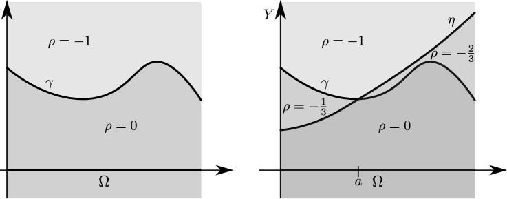
Figure 1: The left-hand side diagram illustrates the values of $\rho$ when $\mu$ is induced by a single curve $\gamma$. In the right-hand side, we illustrate the case in which $\mu$ is the convex combination $\mu=\frac{2}{3}\mu_{1}+\frac{1}{3}\mu_{2}$ and $\mu_{1}$ and $\mu_{2}$ are measures induced by two curves, $\gamma$ and $\eta$, respectively.

After checking that $\rho$ is bounded (Lemma 2.13), we will use the function $\rho$ to define the functions $\varphi_{r}$ (commonly known as sheets) that will give the decomposition of $\mu$. This is done in Lemma 2.15. Lemma 2.17 shows that $\varphi_{r}$ roughly corresponds to the boundary of a level set of $\rho$, and that it is “almost continuous,” and Lemma 2.19 shows that it is weakly differentiable; these two lemmas are used to prove Lemma 2.15. The proof of Theorem 2.2, presented at the end of Section 2.3.2, relies on the fundamental identity above, together with the technical details from Lemma 2.15.

In our example, the decomposition of Theorem 2.2 gives the measure $\nu$ equal to Lebesgue measure on $I=[-1,0]$, and

$$\varphi_{r}(x)=\inf_{\begin{subarray}{c}y\in Y\\ \rho(x,y)\leq r\end{subarray}}y=\gamma(x),\quad r\in[-1,0),$$

so that, indeed,

$$\int_{\Omega\times Y\times Z}f\,d\mu=\int_{I}\int_{\Omega}f(x,\varphi_{r}(x),D\varphi_{r}(x))\,dx\,d\nu(r)\\ =\int_{-1}^{0}\int_{0}^{1}f(x,\gamma(x),\gamma^{\prime}(x))\,dx\,d\nu(r)=\int_{0}^{1}f(x,\gamma(x),\gamma^{\prime}(x))\,dx.$$

Another example, illustrated as well in Figure 1, is the case in which $\mu=\tfrac{2}{3}\mu_{1}+\tfrac{1}{3}\mu_{2}$, and $\mu_{1}$ and $\mu_{2}$ are the measures induced by curves $\gamma$ and $\eta$, and say that $\gamma\geq\eta$ on $[0,a]$ and $\gamma<\eta$ on $(a,1]$, for some $0<a<1$. In this case,

$$\rho(x,y)=\begin{cases}0,&y<\gamma(x)\;\textrm{and}\;y<\eta(x),\\ -\tfrac{1}{3},&\eta(x)\leq y<\gamma(y),\\ -\tfrac{2}{3},&\gamma(x)\leq y<\eta(y),\\ -1,&y\geq\gamma(x)\;\textrm{and}\;y\geq\eta(x).\end{cases}$$

Similarly,

$$\varphi_{r}(x)=\begin{cases}\gamma(x),&\textrm{($-1<r<-\tfrac{1}{3}$ and $0<x<a$) or ($-\tfrac{2}{3}<r<0$ and $a<x<1$)},\\ \eta(x),&\textrm{($-\tfrac{1}{3}<r<0$ and $0<x<a$) or ($-1<r<-\tfrac{2}{3}$ and $a<x<1$)}.\end{cases}$$

2.3.2 Proof of Theorem 2.2

We collect some lemmas needed in the proof of the theorem, which is presented at the end of the section. Throughout this section, we assume that $\mu$ is a measure satisfying the hypotheses of Theorem 2.2.

Lemma 2.9.

If $\pi_{\Omega}{}\colon\Omega\times Y\times Z\to\Omega$ is the projection, then there is $c>0$ such that

$$(\pi_{\Omega}{})_{\#}\mu=c\,dx.$$

In other words, the pushforward $(\pi_{\Omega}{})_{\#}\mu$ is a positive multiple of the Lebesgue measure on $\Omega$.

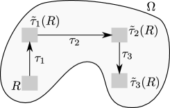
Figure 2: Translating a rectangle in the proof of Lemma 2.9.

Proof.

Let $R\subset\Omega$ be a small parallelepiped, and let $\tau$ be a translation such that $\tau(R)\subset\Omega$. We will show that $(\pi_{\Omega}{})_{\#}\mu(R)=(\pi_{\Omega}{})_{\#}\mu(\tau(R))$, and since this will be true for all $R$ and all $\tau$, $(\pi_{\Omega}{})_{\#}\mu$ must be a positive multiple of Lebesgue on $\Omega$ [21, Thm. 2.20]. Write $\tau$ as a finite composition of translations $\tau_{i}$ in the directions of the axes $x_{1},\dots,x_{n}$,

$$\tau=\tau_{k}\circ\tau_{k-1}\circ\dots\circ\tau_{1}.$$

Denote $\tilde{\tau}_{i}=\tau_{i}\circ\tau_{i-1}\circ\dots\circ\tau_{1}$ and set $\tilde{\tau}_{0}$ equal to the identity. We assume $\tau_{1},\dots,\tau_{k}$ have been chosen also in a such a way that the convex hull of $\tilde{\tau}_{i-1}(R)\cup\tilde{\tau}_{i}(R)$ is contained in $\Omega$ for each $i$. Refer to Figure 2. For each $i=1,\dots,k$, let $j_{i}$ be such that $\tau_{i}$ is a translation in direction $x_{j_{i}}$. Recall that $\chi_{\tilde{\tau}_{i}(R)}$ is the indicator function of the translated rectangle $\tilde{\tau}_{i}(R)$, and let

$$\phi_{i}(x_{1},\dots,x_{n})=\int_{-\infty}^{x_{j_{i}}}\chi_{\tilde{\tau}_{i}(R)}(x_{1},\dots,x_{j_{i}-1},s,x_{j_{i}+1},\dots,x_{n})\\ -\chi_{\tilde{\tau}_{i-1}(R)}(x_{1},\dots,x_{j_{i}-1},s,x_{j_{i}+1},\dots,x_{n})ds.$$

Observe that

$$\operatorname{supp}\phi_{i}=\overline{\operatorname{conv}}(\tilde{\tau}_{i-1}(R)\cup\tilde{\tau}_{i}(R)),$$

which is a compact set properly contained in $\Omega$. Approximating with smooth, compactly-supported functions and using the Lebesgue dominated convergence theorem, we conclude that (11) is true for $\phi_{i}$, which means, for the $j_{i}^{\mathrm{th}}$ entry,

$$(\pi_{\Omega}{})_{\#}\mu(\tilde{\tau}_{i}(R))-(\pi_{\Omega}{})_{\#}\mu(\tilde{\tau}_{i-1}(R))=\int_{\Omega\times Y\times Z}\chi_{\tilde{\tau}_{i}(R)}-\chi_{\tilde{\tau}_{i-1}(R)}\,d\mu\\ =\int_{\Omega\times Y\times Z}\frac{\partial\phi_{i}}{\partial x_{j_{i}}}\,d\mu=\int_{\Omega\times Y\times Z}\frac{\partial\phi_{i}}{\partial x_{j_{i}}}+\frac{\partial\phi_{i}}{\partial y}z_{j_{i}}\,d\mu=0.$$

By induction we get

$$(\pi_{\Omega}{})_{\#}\mu(R)=(\pi_{\Omega}{})_{\#}\mu(\tilde{\tau}_{0}(R))=(\pi_{\Omega}{})_{\#}\mu(\tilde{\tau}_{k}(R))=(\pi_{\Omega}{})_{\#}\mu(\tau(R)).\qed$$

For a vector field $X\colon\Omega\times Y\to\mathbb{R}^{n+1}$, we can define

$$\mu(X)\coloneqq\int\langle X(x,y),(z_{1},\dots,z_{n},-1)\rangle\,d\mu(x,y,z).$$ (26)

When $\mu$ is induced by a smooth function $\varphi\colon\Omega\to Y$, $\mu(X)$ is the circulation of $X$ through the graph of $\varphi$, since $(z_{1},\dots,z_{n},-1)=(\frac{\partial\varphi}{\partial x_{1}},\dots,\frac{\partial\varphi}{\partial x_{n}},-1)$ is normal to that graph of $\varphi$.

Lemma 2.10.

Let $X\colon\Omega\times Y\to\mathbb{R}^{n+1}$ be a smooth, compactly-supported vector field that vanishes on a neighborhood of $\partial\Omega\times Y$ and satisfies $\operatorname{div}X=0.$ Then

$$\mu(X)=0.$$

Proof.

Let

$$\tilde{X}_{i}(x,y)=\int_{-\infty}^{y}X_{i}(x,s)ds.$$ (27)

Then $\tilde{X}_{i}\in C^{\infty}(\Omega\times Y)$ and vanishes on $\partial\Omega\times Y$, so by the $i$-th entry of (11), with $\phi=\tilde{X}_{i}$,

$$\int_{\Omega\times Y\times Z}\left(\frac{\partial\tilde{X}_{i}}{\partial x_{i}}(x,y)+X_{i}(x,y)z_{i}\right)d\mu(x,y,z)=0.$$

Rearranging, and plugging this into the definition of $\mu(X)$, it follows that

$$\mu(X) =\sum_{i=1}^{n}\int_{\Omega\times Y\times Z}X_{i}(x,y)z_{i}\,d\mu(x,y,z)-\int_{\Omega\times Y\times Z}X_{n+1}(x,y)d\mu(x,y,z)$$

$$=-\int_{\Omega\times Y\times Z}\sum_{i=1}^{n}\frac{\partial\tilde{X}_{i}}{\partial x_{i}}(x,y)+X_{n+1}(x,y)\,d\mu(x,y,z)$$

Now, using (27) and

$$X_{n+1}(x,y)=\int_{-\infty}^{y}\frac{\partial X_{n+1}}{\partial x_{n+1}}(x,s)\,ds,$$

we get

$$\sum_{i=1}^{n}\frac{\partial\tilde{X}_{i}}{\partial x_{i}}+X_{n+1}=\int_{-\infty}^{y}\sum_{i=1}^{n+1}\frac{\partial X_{i}}{\partial x_{i}}(x,s)\,ds=\int_{-\infty}^{y}\operatorname{div}X\,ds,$$

which vanishes by the assumption that $\operatorname{div}X=0$. ∎

We define, for measurable, compactly supported, and bounded functions $u\colon\Omega\times Y\to\mathbb{R}$,

$$S(u) =\mu\left(0,\dots,0,\int_{y}^{\infty}u(x,s)ds\right)$$

$$=-\int\left(\int_{y}^{\infty}u(x,s)ds\right)\,d\mu(x,y,z).$$ (28)

Lemma 2.11.

The functional $S$ corresponds to integration with respect to an absolutely continuous nonpositive measure; in other words, there is a measurable function $\rho\colon\Omega\times Y\to(-\infty,0]$ such that

$$S(u) =\int_{\Omega\times Y}u(x,y)\rho(x,y)\,dx\,dy$$

Proof.

This follows from the Radon-Nikodym theorem. To apply the theorem we need to check that, if $A\subset\Omega\times Y$ is a set of measure zero and $\chi_{A}$ is its indicator function, then $S(\chi_{A})=0$. Indeed, if $A\cap\{(x,y):y\in Y\}$ has zero measure for Lebesgue-almost all $x\in\Omega$, then $\int_{-\infty}^{y}\chi_{A}(x,s)ds=0$ for almost all $x\in\Omega$, and by Lemma 2.9 and the Fubini theorem, the integral in the definition (28) of $S(\chi_{A})$ vanishes. To see that the function $\rho$ can be taken to be nonpositive, observe that whenever $u$ is nonnegative, its primitive also satisfies $\int_{-\infty}^{y}u(x,s)ds\geq 0$, so $S(u)\leq 0$. ∎

Lemma 2.12.

When restricted to a line $\{(x,y):y\in Y\}$, $x\in\Omega$, the function $y\mapsto\rho(x,y)$ is (non-strictly) decreasing for almost every $x\in\Omega$. If $N>0$ is such that $\operatorname{supp}\mu\subset\Omega\times(-N,N)\times Z$, then $y\mapsto\rho(x,y)$ vanishes throughout $(-\infty,N]$ and is constant on $[N,+\infty)$, for almost every $x\in\Omega$.

Observe that, strictly speaking, $\rho$ is only defined Lebesgue-almost everywhere on $\Omega\times Y$, so the statement of the lemma should be interpreted as ascertaining the existence of a representative, in the equivalence class of measurable functions coinciding with $\rho$ Lebesgue-almost everywhere, having the desired properties.

Proof.

Let $R$ be an $(n+1)$-dimensional box in $\Omega\times Y$ whose edges are parallel to the axes, and let $\tau_{t}(x,y)=(x,y+t)$ be the translation in the $y$ direction. Then, by Lemma 2.11 and definitions (26) and (28),

$$\int_{R}\rho(x,y-t)\,dx\,dy =\int_{\tau_{t}(R)}\rho(x,y)\,dx\,dy$$

$$=\int_{\Omega\times Y}\chi_{\tau_{t}(R)}(x,y)\rho(x,y)\,dx\,dy$$

$$=S(\chi_{\tau_{t}(R)})$$

$$=\mu\left(0,\dots,0,\int_{y}^{\infty}\chi_{\tau_{t}(R)}(x,s)ds\right)$$

$$=\mu\left(0,\dots,0,\int_{y-t}^{\infty}\chi_{R}(x,s)ds\right)$$

$$=-\int_{\Omega\times Y\times Z}\left(\int_{y-t}^{\infty}\chi_{R}(x,s)ds\right)d\mu(x,y,z).$$

Since $\mu$ is a positive measure, the last term is nonincreasing in $t$. Since this is true for all $t$ and all $R$, this proves that $\rho$ is nonincreasing in the $y$ direction. This proves the first part of the lemma.

To prove the second statement of the lemma, consider the case in which $R=R_{\Omega}\times[a,b]$ for some box $R_{\Omega}\subset\Omega$ and some $a<b$. Then

$$\int_{y}^{\infty}\chi_{R}(x,s)\,ds=\begin{cases}b-a,&y\leq a,\\ 0,&y\geq b.\end{cases}$$

Thus if $a<b\leq-N$, we have

$$\int_{R}\rho(x,y)\,dx\,dy=-\int_{\Omega\times Y\times Z}\left(\int_{y}^{\infty}\chi_{R}(x,y)\,ds\right)d\mu(x,y,z)=\int_{\Omega\times Y\times Z}0\,d\mu(x,y,z).$$

On the other hand, if $N\leq a<b$, then

$$\int_{R}\rho(x,y)\,dx\,dy=-\int_{\Omega\times Y\times Z}\left(\int_{y}^{\infty}\chi_{R}(x,y)\,ds\right)d\mu(x,y,z)=-\int_{\Omega\times Y\times Z}(b-a)\,d\mu(x,y,z).$$

This is impervious to translations of the interval $[a,b]$. This proves the second statement of the lemma. ∎

Lemma 2.13.

The function $\rho$ in Lemma 2.9 is essentially bounded.

Proof.

Aiming for a contradiction, assume that the function $\rho\leq 0$ is not essentially bounded. Then the sets $B_{j}=\{(x,y)\in\Omega\times Y:\rho(x,y)\leq-j\}$, $j\in\mathbb{N}$, have positive measure. By Lemma 2.12, if we take $N>0$ to be such that $\operatorname{supp}\mu\subset\Omega\times(-N,N)\times Z$, then $y\mapsto\rho(x,y)$ is everywhere non-strictly decreasing and is constant on $[N,+\infty)$ for all $x\in\Omega$. Thus the sets $B_{j}\cap(\Omega\times[N,N+1])$ must have positive measure. Pick a subset $A_{j}\subset\{(x,y)\in\Omega\times[N,N+1]:\rho(x,y)\leq-j\}\subset B_{j}$ of finite measure $|A_{j}|<\infty$ and of the form $A_{j}=A_{j}^{\Omega}\times[N,N+1]$, with $A_{j}^{\Omega}\subseteq\Omega$. Observe that this means that $A_{j}$ does not intersect the compact set $\operatorname{supp}\mu$. Pick an open set $U_{j}\subset\Omega\times Y$, of the same product form, $U_{j}=U^{\Omega}_{j}\times[N,N+1]$, such that $A_{j}\subseteq U_{j}$ with $|U_{j}\setminus A_{j}|\leq|A_{j}|/j$, which is possible due to the outer regularity of Lebesgue measure. Note that the function $f_{j}=\chi_{U_{j}}/|A_{j}|$ verifies $\int_{\Omega\times Y}\rho f_{j}\leq\int_{A_{j}}(-j)f_{j}+\int_{U_{j}\setminus A_{j}}0\,f_{j}=-j$. Take $\phi_{j}\in C^{\infty}_{c}(\Omega\times Y)$ to be any good $C^{\infty}$ approximation of $f_{j}$ that satisfies

$$\int_{\Omega\times Y}\rho\phi_{j}dx\,dy\leq-j/2,$$ (29)

$$|\pi_{\Omega}{}(\operatorname{supp}\phi_{j})|\leq 2|A^{\Omega}_{j}|,$$

$$\sup_{x\in\Omega}\int_{-\infty}^{\infty}\phi_{j}(x,s)ds\leq 2\frac{1}{|A_{j}|}=\frac{2}{|A^{\Omega}_{j}|}.$$

Then we have by Lemma 2.11, (28), the fact that $\mu$ and $\phi_{j}$ are non-negative, the bounds above, and Lemma 2.9,

$$-\frac{j}{2} \geq\int_{\Omega\times Y}\phi_{j}(x,y)\rho(x,y)dx\,dy$$

$$=S(\phi_{j})$$

$$=\mu\left(0,\dots,0,\int_{-\infty}^{y}\phi_{j}(x,s)ds\right)$$

$$=-\int_{\Omega\times Y\times Z}\int_{-\infty}^{y}\phi_{j}(x,s)ds\,d\mu(x,y,z)$$

$$\geq-\int_{\Omega\times Y\times Z}\int_{-\infty}^{\infty}\phi_{j}(x,s)ds\,d\mu(x,y,z)$$

$$\geq-\int_{\Omega\times Y\times Z}\frac{2}{|A^{\Omega}_{j}|}\chi_{\pi_{\Omega}{}(\operatorname{supp}\phi_{j})}(x)d\mu(x,y,z)$$

$$=-\frac{2}{|A^{\Omega}_{j}|}(\pi_{\Omega}{})_{\#}\mu(\pi_{\Omega}{}(\operatorname{supp}\phi_{j}))$$

$$=-\frac{2}{|A^{\Omega}_{j}|}c|\pi_{\Omega}{}(\operatorname{supp}\phi_{j})|$$

$$\geq-\frac{2}{|A^{\Omega}_{j}|}c(2|A^{\Omega}_{j}|)=-4c,$$

where $\pi_{\Omega}{}$ and $c$ are as in the statement of Lemma 2.9. This uniform bound gives the contradiction we were aiming for. We conclude that the essential range of $\rho$ is a bounded interval in $(-\infty,0]$. ∎

We will henceforth take $\rho$ to be bounded (we may choose such a representative in its class of essentially bounded functions) and denote the range of $\rho$ by

$$I=\rho(\Omega\times Y)\subset(-\infty,0].$$

We will also denote by $\nu$ the restriction of Lebesgue measure to $I$.

Lemma 2.14.

For all smooth vector fields $X$ compactly supported in $\Omega\times Y$ and vanishing in a neighborhood of $\partial\Omega\times Y$,

$$\mu(X)=S(\operatorname{div}X).$$

Proof.

Indeed,

$$\operatorname{div} (X-\Big{(}\underbrace{0,\dots,0}_{n},\int_{y}^{\infty}\operatorname{div}X(x,s)\,ds\Big{)})$$

$$=\sum_{i=1}^{n}\frac{\partial}{\partial x_{i}}\left(X_{i}-0\right)+\frac{\partial}{\partial y}\left(X_{n+1}-\int_{y}^{\infty}\operatorname{div}X\,ds\right)$$

$$=\operatorname{div}X-\operatorname{div}X$$

$$=0.$$

By Lemma 2.10,

$$0 =\mu(X-\left(0,\dots,0,\int_{y}^{\infty}\operatorname{div}X\,ds\right))$$

$$=\mu(X)-\mu\left(0,\dots,0,\int_{y}^{\infty}\operatorname{div}X\,ds\right)$$

$$=\mu(X)-S(\operatorname{div}X).\qed$$

Lemma 2.15.

The functions $\varphi_{r}:\Omega\to\mathbb{R}$ defined by,

$$\varphi_{r}(x)=\inf_{\begin{subarray}{c}y\in Y\\ \rho(x,y)\leq r\end{subarray}}y,\qquad r\in I=\rho(\Omega\times Y)\subseteq(-\infty,0],\;x\in\Omega,$$

are weakly differentiable. These functions satisfy, for all $X\in C^{\infty}_{c}(\Omega\times Y;\mathbb{R}^{n+1})$,

$$\int_{I}\int_{\{(x,y)\in\Omega\times Y:y\geq\varphi_{r}(x)\}}\operatorname{div}X\,dx\,dy\,d\nu(r)=\int_{I}\int_{\Omega}\langle X(x,\varphi_{r}(x)),(D\varphi_{r}(x),-1)\rangle\,dx\,d\nu(r),$$ (30)

where $\nu$ is Lebesgue measure restricted to $I$.

Observe that, since by Lemma 2.13 $\rho$ is essentially bounded, we may take a representative in the class of $\rho$ that is bounded, and then $\varphi_{r}(x)$ is finite for each $x\in\Omega$.

Proof.

Consider the set $C^{1}_{c}(\Omega\times Y;\mathbb{R}^{n+1})$ of compactly-supported vector fields that are continuously differentiable. Observe that since these vector fields are compactly supported, they vanish on the boundary $\partial\Omega\times Y$. Consider also the set $B$ of vector fields $X\in C^{1}_{c}(\Omega\times Y;\mathbb{R}^{n+1})$ satisfying $\sup_{\Omega\times Y}\|X(x,y)\|\leq 1$.

Since we have a uniform bound, by (9), for $X\in B$, by Lemma 2.11, (28), Lemma 2.14, (26), the Cauchy-Schwarz inequality, and the finiteness of $\mu$ together with (9),

$$\left|\int\rho\operatorname{div}X\,dx\,dy\right|=S(\operatorname{div}X)=\mu(X)=\\ \left|\int\langle X(x,y),(z,-1)\rangle\,d\mu(x,y,z)\right|\leq\int 1+\|z\|\,d\mu(x,y,z)<+\infty,$$

we conclude that $\rho$ is a function of bounded variation (see [6, Def. 5.1]) in $\Omega\times Y$. It follows from the coarea formula [6, Thm. 5.9] that there is a set of full measure $A\subset I$, $|I\setminus A|=0$, such that if $r\in A$ then $\rho^{-1}(-\infty,r]\subset\Omega\times Y$ is a set of locally finite perimeter ([6, Def. 5.1], [16, Ch. 12]), meaning that

$$\sup_{X\in B}\int_{\rho^{-1}(-\infty,r]}\operatorname{div}X(x,y)\,dx\,dy<+\infty,\quad r\in A.$$

By [16, Prop. 12.1], there exists an $\mathbb{R}^{n+1}$-valued measure $\bm{\nu}_{r}$ with bounded total variation $|{\bm{\nu}}_{r}|$ (defined in [16, Rmk. 4.12]), $|{\bm{\nu}}_{r}|(\overline{\Omega\times Y})<+\infty$, such that, for $X\in C^{1}_{c}(\Omega\times Y;\mathbb{R}^{n+1})$,

$$\int_{\rho^{-1}(-\infty,r]}\operatorname{div}X\,dx\,dy=\int_{\Omega\times Y}X\cdot d{\bm{\nu}}_{r}=\sum_{i=1}^{n+1}\int_{\Omega\times Y}X_{i}d{\bm{\nu}}_{r,i}$$

De Giorgi’s Structure Theorem ([6, Th. 5.15 and 5.16] or [16, Th. 15.9]) then implies that ${\bm{\nu}}_{r}$ is supported on the boundary $\partial\rho^{-1}(-\infty,r]$, that this boundary is of Hausdorff dimension $n$, and that the unit normal $\eta_{r}$ to the boundary of $\rho^{-1}(-\infty,r]$ is well defined for almost every point $(x,y)$ on the boundary with respect to Hausdorff measure $H^{n}$ of dimension $n$ by

$$\eta_{r}(x,y)=\lim_{b\searrow 0}\frac{{\bm{\nu}}_{r}(D((x,y),b))}{|{\bm{\nu}}_{r}|(D((x,y),b))}$$ (31)

where $D((x,y),b)$ denotes the ball centered at $(x,y)$ of radius $b>0$ and $|{\bm{\nu}}_{r}|$ denotes the total variation of ${\bm{\nu}}_{r}$. Refer to Figure 3.

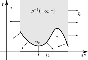
Figure 3: The sets $\rho^{-1}(-\infty,r]$ and their exterior unit normal $\eta_{r}$, as in the situation of Lemma 2.15.

Also, the Gauss-Green formula holds: for $X\in C^{1}(\overline{\Omega\times Y},\mathbb{R}^{n+1})$,

$$\int_{\rho^{-1}(-\infty,r]}\operatorname{div}X\,dx\,dy=\int_{\partial\rho^{-1}(-\infty,r]}\langle X,\eta_{r}\rangle dH^{n}.$$ (32)

Indeed, this is equivalent to [16, eq. (15.11)], summing over all the entries in that vector-valued equation; cf. [16, Rmk. 12.2].

From Lemma 2.17 below and Remark 2.18, it follows that $H^{n}$-almost all the boundary $(\partial\rho^{-1}(-\infty,r])\cap(\Omega\times Y)$ corresponds to the image of $\varphi_{r}$, i.e.,

$$H^{n}((\partial\rho^{-1}(-\infty,r])\cap(\Omega\times Y)\setminus\{(x,\varphi_{r}(x)):x\in\Omega\})=0.$$

Let $\zeta_{r}\colon\Omega\to\mathbb{R}^{n}$ be the vector field whose $i$-th entry is given by

$$[\zeta_{r}(x)]_{i}=-\frac{[\eta_{r}(x,\varphi_{r}(x))]_{i}}{[\eta_{r}(x,\varphi_{r}(x))]_{n+1}},\quad 1\leq i\leq n,$$ (33)

if the denominator is $\neq 0$, and $[\zeta_{r}(x)]_{i}=\operatorname{sign}([\eta_{r}(x)]_{i})\infty$ otherwise. It follows from Lemma 2.19 below that the denominator in (33) is almost-everywhere nonzero, and that $\zeta_{r}$ is the weak derivative of $\varphi_{r}$.

Equality (30) follows from

$$\int_{I}\int_{\{y\geq\varphi_{r}(x)\}}\operatorname{div}X\,dx\,dy\,d\nu(r) =\int_{I}\int_{\partial\rho^{-1}(-\infty,r]}\langle X,\eta_{r}\rangle dH^{n}\,d\nu(r)$$

$$=\int_{I}\int_{\Omega}\langle X(x,\varphi_{r}(x)),(\zeta_{r}(x),-1)\rangle dx\,d\nu(r),$$

which is Lemma 2.19(ii), together with $\zeta_{r}$ being the weak derivative $D\varphi_{r}$. ∎

Lemma 2.16.

If $r\leq r^{\prime}\leq 0$ and $x_{0}\in\Omega$ is such that $\varphi_{r}(x_{0})=\varphi_{r^{\prime}}(x_{0})$ and $\eta_{r}$ and $\eta_{r^{\prime}}$ are defined at $x_{0}$, then $\eta_{r}(x,\varphi_{r}(x_{0}))=\eta_{r^{\prime}}(x,\varphi_{r^{\prime}}(x_{0}))$.

Proof.

This follows immediately from [6, Th. 5.13]. ∎

Lemma 2.17.

For $r\in I$, let $P_{r}$ be the set of points $x\in\Omega$ such that there is exactly one value $y\in Y$ such that $(x,y)\in\partial\rho^{-1}(-\infty,r]$. For almost every $r\in I$, the $(n-1)$-dimensional Hausdorff volume of the complement of $P_{r}$ is

$$H^{n-1}(\Omega\setminus P_{r})=0.$$

Remark 2.18.

The statement of Lemma 2.17 means that the graph of the function $\varphi_{r}$ defined in the statement of Lemma 2.15 coincides with $(\partial\rho^{-1}(-\infty,r])\cap\Omega\times Y$ almost everywhere.

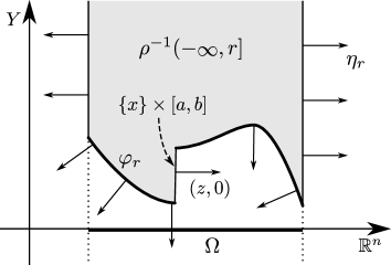
Figure 4: When there is a vertical segment $\{x\}\times[a,b]$ in the boundary $\partial\rho^{-1}(-\infty,r]$, the normal vector is horizontal, that is, of the form $(z,0)$, $z\in\mathbb{R}^{n}$. The proof of Lemma 2.17 shows that the $n$-dimensional volume of the union of these segments is zero.

Proof.

From the boundedness of $\rho$ (Lemma 2.13 it follows that at least one such value $y$ exists. Since $\rho$ is non-increasing (Lemma 2.12, given $x\in\Omega$ the set of values $y\in Y$ with $(x,y)\in\partial\rho^{-1}(-\infty,r]$ must be an interval.

We will show that, for almost all $r\in I$, the normal vector $\eta_{r}$ is almost nowhere with respect to Hausdorff measure $H^{n}|_{\rho^{-1}(-\infty,r]}$ of the form $(z,0)$ for some $z\in\mathbb{R}^{n}$; the $0$ in the $Y$ direction appears every time the boundary $\partial\rho^{-1}(-\infty,r]$ contains a segment of the form $\{x\}\times[a,b]\subset\Omega\times Y$ with $a<b$, as vectors tangent to such a segment are of the form $(0,\dots,0,a)$, $0\neq a\in\mathbb{R}$, and $\eta_{r}$ is perpendicular to them; refer to Figure 4. In other words, we will show that the $n$-dimensional Hausdorff volume of the union of intervals of the form $\{x\}\times[a,b]$ in the boundary $\partial\rho^{-1}(-\infty,r]$ is zero; its projection onto $\Omega$ is $\Omega\setminus P_{r}$, whence this implies the statement of the lemma.

Denoting the last entry of the vector field $\eta_{r}$ by $[\eta_{r}]_{n+1}$, we let $A_{r}$ be the set of points $(x,y)\in\partial\rho^{-1}(-\infty,r]\subseteq\Omega\times Y$ where $[\eta_{r}]_{n+1}(x,y)=0$.

By Lemmas 2.11 and 2.14 as well as definitions (26) and (28),

$$\int_{I}\int_{\partial\rho^{-1}(-\infty,r]}\langle X,\eta_{r}\rangle dH^{n}\,d\nu(r) =\int_{I}\left(\int_{\rho^{-1}(-\infty,r]}\operatorname{div}X\,dx\,dy\right)\,d\nu(r)$$

$$=\int\rho\operatorname{div}X\,dx\,dy$$

$$=S(\operatorname{div}X)$$

$$=\mu(X)$$

$$=\int_{\Omega\times Y\times Z}\langle X(x,y),(z,-1)\rangle\,d\mu(x,y,z)$$ (34)

for all $X\in C^{1}_{c}(\Omega\times Y;\mathbb{R}^{n+1})$. By the density of $C^{1}_{c}(\Omega\times Y;\mathbb{R}^{n})$ in $L^{1}((\pi_{\Omega\times Y})_{\#}\mu;\mathbb{R}^{n})$ and dominated convergence, this holds as well for vector fields $X$ in the latter space.

Let $X=(0,\chi_{A})$, with $A=\bigcup_{r}A_{r}$. Then, by (34),

$$-\mu(A)= -\int_{\Omega\times Y\times Z}\chi_{A}(x,y)d\mu(x,y,z)$$

$$=\int_{\Omega\times Y\times Z}\langle X(x,y),(z,-1)\rangle\,d\mu(x,y,z)$$

$$=\int_{I}\int_{\partial\rho^{-1}(-\infty,r]}\langle X,\eta_{r}\rangle\,dH^{n}\,d\nu(r)$$

$$=\int_{I}\int_{\partial\rho^{-1}(-\infty,r]}\chi_{A}[\eta_{r}]_{n+1}\,dH^{n}\,d\nu(r)=0,$$

since $[\eta_{r}]_{n+1}(x,y)=0$ whenever $(x,y)\in A_{r}$, and by Lemma 2.16 this happens whenever $(x,y)\in A$ because $\eta_{r}(x,y)$ is independent of $r$ (among those values of $r$ such that $(x,y)\in\partial\varphi^{-1}(-\infty,r]$). Then we have, again using (34) and $\|\eta_{r}\|=1$,

$$\int_{I}\int_{\partial\rho^{-1}(-\infty,r]}\chi_{A}\,dH^{n}\,d\nu(r)=\int_{I}\int_{\partial\rho^{-1}(-\infty,r]}\langle\chi_{A}\eta_{r},\eta_{r}\rangle\,dH^{n}\,d\nu(r)\\ =\int_{\Omega\times Y\times Z}\chi_{A}\langle\eta_{r},(z,-1)\rangle\,d\mu(x,y,z)=0.$$

This is what we wanted to show. ∎

Lemma 2.19.

1. The vector field $\zeta_{r}$ defined in (33) is the weak derivative of $\varphi_{r}$, that is,

   $$\int_{\Omega}\varphi_{r}(x)\nabla\phi(x)\,dx=\int_{\Omega}\phi(x)\zeta_{r}(x)\,dx$$

   for all $\phi\in C^{\infty}_{c}(\Omega)$.

2. We also have, for $X\in C^{1}_{c}(\Omega\times Y;\mathbb{R}^{n+1})$, and for almost every $r\leq 0$,

   $$\int_{\partial\rho^{-1}(-\infty,r]}\langle X,\eta_{r}\rangle dH^{n}=\int_{\Omega}\langle X(x,\varphi_{r}(x)),(\zeta_{r}(x),-1)\rangle dx.$$

Proof.

For almost every $r\in(-\infty,0]$, $\eta_{r}$ is well defined on almost all the boundary $\partial\rho^{-1}(-\infty,r]$.

Denote by $m_{1}^{r}$ the Hausdorff measure $H^{n}$ on the boundary $(\partial\rho^{-1}(-\infty,r])\cap(\Omega\times Y)$ (since $\Omega$ is open, this is just the graph of $\varphi_{r}$; see Figure 3), and by $m_{2}^{r}$ the pushforward of Lebesgue measure on $\Omega$ by the map $x\mapsto(x,\varphi_{r}(x))$; $m_{2}^{r}$ is also supported in $(\partial\rho^{-1}(-\infty,r])\cap(\Omega\times Y)$. The measure $m_{2}^{r}$ is absolutely continuous with respect to $m_{1}^{r}$. Indeed, if $A$ is a measurable set of zero $m_{1}^{r}$ measure, this means that for every $\varepsilon>0$, $A$ can be covered with finitely many balls $U_{1},\dots,U_{k}$ such that $\sum_{i=1}^{k}(\operatorname{diam}U_{k})^{n}\leq\varepsilon$. The image $\pi_{\Omega\times Y}{}(A)$ through the projection $\pi_{\Omega\times Y}{}\colon\Omega\times Y\to\Omega$ can then be covered by the projections of the balls $\pi_{\Omega\times Y}{}(U_{i})$, which will still satisfy (for some $C>0$ dependent only on $n$)

$$m^{r}_{2}(A)\leq m^{r}_{2}({\textstyle\bigcup_{i=1}^{k}U_{i}})\leq|\textstyle\bigcup_{i=1}^{k}\pi_{\Omega\times Y}{}(U_{i})|\leq C\sum_{i=1}^{k}(\operatorname{diam}\pi_{\Omega\times Y}{}(U_{i}))^{n}\leq\varepsilon,$$

and hence $A$ is a set of measure zero with respect to $m^{2}_{k}$. This proves the absolute continuity of $m^{2}_{k}$ with respect to $m_{1}^{r}$.

By the Radon-Nikodym theorem there is a measurable function $J_{r}(x,y)$ such that for all measurable functions $f\colon\Omega\times Y\times Z\to\mathbb{R}$,

$$\int_{\partial\rho^{-1}(-\infty,r]}f(x,y)\eta_{r}(x,y)\,dH^{n}=\int_{\partial\rho^{-1}(-\infty,r]}f(x,y)\eta_{r}(x,y)\,dm^{r}_{1}\\ =\int_{\partial\rho^{-1}(-\infty,r]}f(x,y)\eta_{r}(x,y)J_{r}(x,y)\,dm_{2}^{r}\\ =\int_{\Omega}f(x,\varphi_{r}(x))\eta_{r}(x,\varphi_{r}(x))J_{r}(x,\varphi_{r}(x))dx.$$ (35)

From (32) it follows that

$$\int_{\{y\geq\varphi_{r}(x)\}}\operatorname{div}X\,dx\,dy=\int_{\partial\rho^{-1}(-\infty,r]}\langle X,\eta_{r}\rangle dH^{n},\quad X\in C^{\infty}_{c}(\overline{\Omega\times Y};\mathbb{R}^{n+1}),$$

or equivalently, we have the vector-valued identity (proved from the above by taking $X=\phi\,e_{i}$ for each vector $e_{i}$ in the standard basis)

$$\int_{\{y\geq\varphi_{r}(x)\}}\nabla\phi(x,y)\,dx\,dy=\int_{\partial\rho^{-1}(-\infty,r]}\phi\,\eta_{r}\,dH^{n},\quad\phi\in C^{\infty}_{c}(\overline{\Omega\times Y};\mathbb{R}).$$ (36)

Take $N>0$ large enough that $\operatorname{supp}\mu\subset\Omega\times[-N,N$, and take a function $\psi\in C^{\infty}_{c}(\overline{\Omega\times Y})$, $0\leq\psi\leq 1$, such that $\psi(x,y)=1$ for all $|y|\leq N$. Then, if we let $\mathbf{n}$ denote the unit normal to the boundary of $\Omega\times[0,+\infty)\subset\Omega\times Y$, using (35), and computing the derivatives below as in $\Omega\times Y$, so that for example $\nabla\phi(x)=\nabla_{x,y}\phi(x)=(\frac{\partial\phi}{\partial x_{1}},\dots,\frac{\partial\phi}{\partial x_{n}},0)$ to account for $\frac{\partial\phi}{\partial y}=0$, we have

$$\int_{\Omega} \varphi_{r}(x)\nabla\phi(x)\,dx=\int_{\Omega}\int_{0}^{\varphi_{r}(x)}\nabla\phi(x)\,dy\,dx$$

$$=\int_{\Omega}\int_{0}^{\varphi_{r}(x)}\nabla(\psi\phi)(x,y)\,dy\,dx$$

$$=\int_{\{(x,y)\in\Omega\times Y:0\leq y\leq\varphi_{r}(x)\}}\nabla(\psi\phi)\,dx\,dy-\int_{\{(x,y)\in\Omega\times Y:0\geq y\geq\varphi_{r}(x)\}}\nabla(\psi\phi)\,dx\,dy$$

$$=\int_{\{(x,y)\in\Omega\times Y:y\geq 0\}}\nabla(\psi\phi)\,dx\,dy-\int_{\{(x,y)\in\Omega\times Y:y\geq\varphi_{r}(x)\}}\nabla(\psi\phi)\,dx\,dy$$

$$=\int_{\partial\{(x,y)\in\Omega\times Y:y\geq 0\}}\psi\phi\mathbf{n}\,dH^{n}-\int_{\partial\rho^{-1}(-\infty,r]}\psi\phi\eta_{r}\,dH^{n}$$

$$=\int_{\Omega\times\{0\}}\phi\mathbf{n}\,dH^{n}-\int_{\{(x,\varphi_{r}(x)):x\in\Omega\}}\phi\eta_{r}\,dH^{n}$$

$$=\int_{\Omega}\phi(x)e_{n+1}dx+\int_{\Omega}\phi(x)\eta_{r}(x)J_{r}(x,\varphi_{r}(x))dx$$

for all $\phi\in C^{\infty}_{c}(\Omega;\mathbb{R})$; here, we have first used the fact that $\varphi_{r}(x)=\int_{0}^{\varphi_{r}(x)}dy$. Then we introduced $\psi$, and we separated the positive and negative parts of $\varphi_{r}$. We have expressed them in a slightly different form (see Figure 5), and then passed to the boundary using (36) and its equivalent for the domain $\{y\geq 0\}\subset\overline{\Omega\times Y}$. In the next-to-last line we used that $\psi=1$ in the region whre the domain of integration and we have kept only the parts that do not cancel out from the fact that $\phi$ is compactly supported in $\Omega$, namely, the sets $\Omega\times\{0\}\subset\partial\{y\geq 0\}$, whose normal is $e_{n+1}$, and $\varphi_{r}(\Omega)$, whose normal is $\eta_{r}$; $J_{r}(x)$ comes in once we apply (35). In other words, we have

$$\int_{\Omega}\varphi_{r}(x)\begin{pmatrix}\nabla_{x}\phi(x)\\ 0\end{pmatrix}dx=\int_{\Omega}\phi(x)e_{n+1}dx+\int_{\Omega}\phi(x)\eta_{r}(x)J_{r}(x,\varphi_{r}(x))dx,$$ (37)

where the 0 entry in the left-hand side appears because $\phi$ is independent of $y$. The last entry of (37) gives

$$0=\int_{\Omega}\phi(x)1\,dx+\int_{\Omega}\phi(x)[\eta_{r}(x,\varphi_{r}(x))]_{n+1}J_{r}(x,\varphi_{r}(x))\,dx.$$

Since this is true for all $\phi\in C^{\infty}_{c}(\Omega)$, we conclude that, for almost every $x\in\Omega$,

$$J_{r}(x,\varphi_{r}(x))=-\frac{1}{[\eta_{r}(x,\varphi_{r}(x))]_{n+1}},$$

and (35) becomes (cf. (33))

$$\int_{\partial\rho^{-1}(-\infty,r]}f(x,y)\eta_{r}(x,y)\,dH^{n}(x,y)=\int_{\Omega}f(x,\varphi_{r}(x))\ \begin{pmatrix}\zeta_{r}(x)\\ -1\end{pmatrix}dx.$$ (38)

Applying (38) to $f=X_{i}$ and adding over all $i=1,\dots,n$ proves the identity in item (ii).

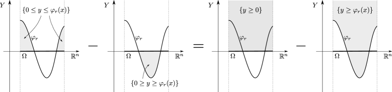
Figure 5: Illustrating a step in the proof of Lemma 2.19, we see that the difference of integrals on the shaded areas in the first two diagrams on the left is equal to the difference of integrals on the the two areas on the right.

We also have, taking only the first $n$ entries in (37),

$$\int_{\Omega}\varphi_{r}(x)\nabla\phi(x)\,dx=\int_{\Omega}\phi(x)\zeta_{r}(x)\,dx.$$

This is precisely the definition (5) of weak differentiability. ∎

Proof of Theorem 2.2.

Let $\phi\colon\Omega\times Y\times Z\to\mathbb{R}$ be, for now, a smooth function that is linear in $z$ and is compactly-supported in $\Omega\times Y$, vanishing in a neighborhood of $\partial\Omega\times Y$.

By Lemma 2.13, the function $\rho$ from Lemma 2.11 is bounded; its range is the bounded interval $I\subseteq\mathbb{R}$. The functions $\varphi_{r}$ in Lemma 2.15 are defined only for $r\in I$. Let $\nu$ denote the restriction of Lebesgue measure to $I$.

Since $\phi$ is linear in $z$, for each $(x,y)\in\Omega\times Y$ the functional $z\mapsto\phi(x,y,z)$ corresponds to a vector $\tilde{X}(x,y)\in\mathbb{R}^{n}$ satisfying

$$\phi(x,y,z)=\langle\tilde{X}(x,y),z\rangle,\quad(x,y,z)\in\Omega\times Y\times Z,$$

and we let $X(x,y)=(\tilde{X}(x,y),0)\in\mathbb{R}^{n+1}$.

Then by Lemmas 2.14 and 2.15 we have

$$\int_{\Omega\times Y\times Z}\phi\,d\mu =\int_{\Omega\times Y\times Z}\langle X,(z,-1)\rangle\,d\mu$$

$$=\mu(X)$$

$$=S(\operatorname{div}X)$$

$$=\int_{\Omega\times Y}\rho\operatorname{div}X\,dx\,dy$$

$$=\int_{I}\int_{\rho^{-1}(-\infty,r]}\operatorname{div}X\,dx\,dy\,d\nu(r)$$

$$=\int_{I}\int_{\{(x,y)\in\Omega\times Y:y\geq\varphi_{r}(x)\}}\operatorname{div}X\,dx\,dy\,d\nu(r)$$

$$=\int_{I}\int_{\Omega}\langle X(x,\varphi_{r}(x)),(D\varphi_{r}(x),-1)\rangle\,dx\,d\nu(r)$$

$$=\int_{I}\int_{\Omega}\phi(x,\varphi_{r}(x),D\varphi_{r}(x))\,dx\,d\nu(r)$$

Thus the first statement of the theorem is true in the case of smooth $\phi$ linear in $z$. Defining $\mathcal{Z}$, $\bar{\mu}$, and $\mu_{xy}$ as in (21) we have for all continuous functions $\phi\colon\Omega\times Y\times Z\to\mathbb{R}$ that are linear in $z$,

$$\int_{\Omega\times Y\times Z}\phi\,d\bar{\mu}=\int_{\Omega\times Y\times Z}\phi\,d\mu=\int_{\mathbb{R}}\int_{\Omega}\phi(x,\varphi_{r}(x),D\varphi_{r}(x))\,dx\,d\nu(r).$$ (39)

This means that for $(\pi_{\Omega\times Y})_{\#}\mu$-almost every $(x,y)$ we have, by Lemma 2.16, that, if $r$ is such that $\varphi_{r}(x)=y$ then

$$D\varphi_{r}(x)=\mathcal{Z}(x,y).$$ (40)

Observe that, by (3), we have

$$\int_{I}\int_{\Omega}\|D\varphi_{r}\|\,dx\,d\nu(r)=\int_{\Omega\times Y\times Z}\|z\|d\mu<+\infty,$$

whence it follows that for $\nu$-almost every $r$, we have $\varphi_{r}\in W^{1,1}(\Omega)$. The argument used to establish (40) shows that in fact $D\varphi_{r}(x)$ is, for almost every $x$ and $\nu$-almost every $r$, in the convex hull of $\operatorname{supp}\mu\cap\{(x,\varphi_{r}(x),z):z\in Z\}$. Since $\operatorname{supp}\mu$ is compact, this implies that $\varphi_{r}$ is in $W^{1,\infty}(\Omega)$ for $\nu$-almost every $r$.

For $\psi\in C^{\infty}(\Omega\times Y)$ we have, using (40),

$$\int_{\Omega\times Y\times Z}\psi(x,y)\,d\mu(x,y,z)=\int_{\Omega\times Y\times Z}\psi(x,y)\left\langle z,\frac{\mathcal{Z}(x,y)}{\|\mathcal{Z}(x,y)\|^{2}}\right\rangle\,d\mu(x,y)\\ =\int_{I}\int_{\Omega}\psi(x,\varphi_{r}(x))\left\langle D\varphi_{r}(x),\frac{\mathcal{Z}(x,\varphi_{r}(x))}{\|\mathcal{Z}(x,\varphi_{r}(x))\|^{2}}\right\rangle\,dx\,d\nu(r)\\ =\int_{I}\int_{\Omega}\psi(x,\varphi_{r}(x))\,dx\,d\nu(r).$$ (41)

This shows that (12) holds for smooth $\phi$ constant in $z$, whence adding up we get the statement for smooth $\phi$ affine in $z$. This implies that the statement holds also for continuous $\phi$ affine in $z$ by the density of $C^{\infty}$ functions affine in $z$ in the space of continuous functions affine in $z$ in the uniform norm on compact sets.

The case of $\phi\in L_{1}(\mu)$ is proven by the following argument. Let $\mu^{\prime}=\int_{I}(\mathrm{id},\varphi_{r},D\varphi_{r})_{\#}\lambda_{\Omega}\,dr$, where $\lambda_{\Omega}$ is the Lebesgue measure on $\Omega$; that is, $\mu^{\prime}$ is the superposition of the occupation measures generated by the functions $\varphi_{r}$. Then equation (12) reads

$$\int_{\Omega\times Y\times Z}\phi\,d\mu=\int_{\Omega\times Y\times Z}\phi\,d\mu^{\prime}$$

for all $\phi\in L_{1}(\mu)$ affine in $z$. Since the result holds for all continuous $\phi$ affine in $z$ and both $\mu$ and $\mu^{\prime}$ are Radon measures, it follows immediately by a classical density result that the statement holds for all $\phi\in L_{1}(\mu)$ independent of $z$. This implies that the $(x,y)$ marginals $\mu_{\Omega\times Y}$ and $\mu^{\prime}_{\Omega\times Y}$ coincide. It remains to prove the statement with $\phi\in L_{1}(\mu)$ linear in $z$; it suffices to consider $\phi$ of the form $\phi(x,y,z)=f(x,y)z_{k}$ for $f\in L^{1}(\mu_{\Omega\times Y})$ and $1\leq k\leq n$, because a general $\phi$ will be a linear combination of these. We already have, for continuous $f$, the identity

$$\int_{\Omega\times Y\times Z}f(x,y)z_{k}\,d\mu(x,y,z)=\int_{\Omega\times Y\times Z}f(x,y)z_{k}\,d\mu^{\prime}(x,y,z).$$

By the same classical density result cited above applied to the signed Radon measures $z_{k}d\mu$ and $z_{k}d\mu^{\prime}$, this identity holds for $f\in L^{1}(\mu_{\Omega\times Y})$ too. This shows that the result is true for all $\phi\in L_{1}(\mu)$.

The last statement of the theorem follows directly from Lemma 2.15. ∎

2.4 Connection with the original Hardt-Pitts decomposition

The context in which superpositions of the type described in Theorem 2.2 were first developed is that of Geometric Measure Theory, in which the main objects of interest are currents, which are the continuous functionals on the space of smooth differential forms on an open set or a manifold. Just like distributions (continuous functionals on $C^{\infty}_{c}(U)$) can be of order higher than 1, involving integrals of derivatives of the test function, currents can also involve derivatives of the differential forms they are fed. This is why it is interesting to distinguish normal currents, which roughly correspond to currents that can be expressed as integrals over a finite measure, evaluating the differential form on a set of vector fields, and satisfying some additional integrability conditions (see for example [18]). Thus for example, the version of the Hardt-Pitts decomposition described in [26] shows that a normal current of dimension $n$ in $\mathbb{R}^{n+1}$ and associated to a finite measure whose density is a positive $C^{\infty}$ function, and smooth vector fields satisfying an integrability condition, can be expressed as a superposition of so-called rectifiable currents of dimension $n$. These are currents that can be written as a sum of countably many integrals over Lipschitz hypersurfaces. Our result does not require the smoothness assumptions of [26].

Let us explain how to associate a normal current $T_{\mu}$ to the measure $\mu$ that Theorem 2.2 decomposes: for a differential form $\omega$ of order $n$ on $\Omega\times Y$, we let

$$T_{\mu}(\omega)=\int_{\Omega\times Y\times Z}\omega_{(x,y)}(\tiny\begin{pmatrix}1\\ 0\\ \vdots\\ 0\\ z_{1}\end{pmatrix},\begin{pmatrix}0\\ 1\\ \vdots\\ 0\\ z_{2}\end{pmatrix},\dots,\begin{pmatrix}0\\ 0\\ \vdots\\ 1\\ z_{n}\end{pmatrix})\,d\mu(x,y,z).$$

Similarly, to each of the sheets $\varphi_{r}$ we can associate a rectifiable current $R_{r}$ on $\Omega\times Y$ given by

$$R_{r}(\omega)=\int_{\Omega}\omega_{(x,\varphi_{r}(x))}(\tiny\begin{pmatrix}1\\ 0\\ \vdots\\ 0\\ \frac{\partial\varphi_{r}}{\partial x_{1}}(x)\end{pmatrix},\begin{pmatrix}0\\ 1\\ \vdots\\ 0\\ \frac{\partial\varphi_{r}}{\partial x_{2}}(x)\end{pmatrix},\dots,\begin{pmatrix}0\\ 0\\ \vdots\\ 1\\ \frac{\partial\varphi_{r}}{\partial x_{n}}(x)\end{pmatrix})\,dx.$$

Then the main conclusion of Theorem 2.2 can be written as

$$T_{\mu}=\int_{\mathbb{R}}R_{r}d\nu(r),$$

an expression that roughly corresponds to [26, eqs. (2), (8)].

2.5 Proof of Theorem 2.3

In order to prove Theorem 2.3, we need a lemma.

Lemma 2.20.

1. Let $\mu$ be as in the statement of Theorem 2.3. Let $\nu$ and $(\varphi_{r})$ be as in the conclusion of Theorem 2.2. Assume that $L\colon\Omega\times Y\times Z\to\mathbb{R}$ is measurable, and convex in $z$. Then

   $$\int_{\mathbb{R}}\int_{\Omega}L(x,\varphi_{r}(x),D\varphi_{r}(x))\,d\nu\leq\int_{\Omega\times Y\times Z}L\,d\mu.$$

2. Assume, additionally to the previous item, that $\mu_{\partial}$ is as in the statement of Theorem 2.3. Then the restriction of $\varphi_{r}$ to $\partial\Omega$ is a well-defined Lipschitz function, and we have, for all measurable functions $\phi\colon\partial\Omega\times Y\to\mathbb{R}$,

   $$\int_{\partial\Omega\times Y\times Z}\phi(x,y)d\mu_{\partial}(x,y)=\int_{\mathbb{R}}\int_{\partial\Omega}\phi(x,\varphi_{r}(x))d\sigma(x)\,d\nu(r),$$

   where $\sigma$ denotes Hausdorff measure on the boundary $\partial\Omega$. In other words, the decomposition of $\mu$ implies a decomposition of $\mu_{\partial}$.

Proof.

Let us prove item (i). Let $\mathcal{Z}$, $\mu_{\Omega\times Y}$, $\mu_{xy}$, and $\bar{\mu}$ be as in Definition 2.5. It follows from Jensen’s inequality that

$$L(x,y,\mathcal{Z}(x,y))\leq\int_{Z}L(x,y,z)\,d\mu_{xy}(z)$$ (42)

and hence also

$$\int_{\Omega\times Y\times Z}L\,d\bar{\mu}=\int_{\Omega\times Y}L(x,y,\mathcal{Z}(x,y))\,d\mu_{\Omega\times Y}(x,y)\\ \leq\int_{\Omega\times Y}\int_{Z}L(x,y,z)d\mu_{xy}(z)d\mu_{\Omega\times Y}(x,y)=\int_{\Omega\times Y\times Z}L\,d\mu.$$ (43)

Since the integrals of the functions $\phi$ in the statement of Theorem 2.2 with respect to $\mu$ and $\bar{\mu}$ coincide, the decomposition given by the theorem is the same for either of these measures; let $\nu$ be the corresponding measure, and $(\varphi_{r})$ be the corresponding family of functions. Thus by (43), the definition of $\bar{\mu}$, the fact that the $L(x,y,\mathcal{Z}(x,y))$ does not depend on $z$, (41), and (40),

$$\int L\,d\mu \geq\int L\,d\bar{\mu}$$

$$=\int L(x,y,\mathcal{Z}(x,y))\,d\mu_{\Omega\times Y}(x,y)$$

$$=\int L(x,y,\mathcal{Z}(x,y))\,d\mu(x,y,z)$$

$$=\int L(x,\varphi_{r}(x),\mathcal{Z}(x,\varphi_{r}(x)))\,dx\,d\nu(r)$$

$$=\int_{\mathbb{R}}\int_{\Omega}L(x,\varphi_{r}(x),D\varphi_{r}(x))\,dx\,d\nu(r)$$

This proves item (i).

To prove item (ii), note that the set $\Omega$ has a boundary measure $\sigma$ supported on $\partial\Omega$ such that, if $X\in C^{1}(\overline{\Omega};\mathbb{R}^{n})$, then the Gauss theorem holds, that is

$$\int_{\partial\Omega}\langle X(x),\mathbf{n}(x)\rangle\,d\sigma(x)=\int_{\Omega}\operatorname{div}X(x)\,dx,\quad\operatorname{div}X=\sum_{i}\frac{\partial X_{i}}{\partial x_{i}},$$ (44)

where $\mathbf{n}\colon\partial\Omega\to\mathbb{R}^{n}$ is the exterior unit vector normal to $\Omega$. Equivalently, for all $u\in C^{1}(\overline{\Omega};\mathbb{R})$ and all $\phi\in C^{\infty}(\overline{\Omega}\times Y;\mathbb{R})$, taking $X(x)=e_{j}\phi(x,u(x))$ for each $j=1,\dots n$ in (44), we get,

$$\int_{\partial\Omega}\phi(x,u(x))\mathbf{n}(x)\,d\sigma(x)=\int_{\Omega}\frac{\partial\phi}{\partial x}(x,u(x))+\frac{\partial\phi}{\partial y}(x,u(x))Du(x)\,dx.$$ (45)

By the density of smooth functions among the weakly-differentiable ones, and continuity of the integral, (45) holds also for bounded weakly differentiable functions $u$.

Remark that, since $\mu$ is compactly supported, for $\nu$-almost every $r$ the function $\varphi_{r}$ is bounded, as is its weak derivative $D\varphi_{r}$. Thus $\varphi_{r}\in W^{1,\infty}(\overline{\Omega})$, and $\varphi_{r}$ is Lipschitz, as is its restriction to the boundary $\partial\Omega$.

We have, from (8), (39), and (45) with $u=\varphi_{r}$, for $f\in C^{\infty}(\overline{\Omega};\mathbb{R})$,

$$\int_{\partial\Omega\times Y\times Z} f(x,y)\mathbf{n}(x)\,d\mu_{\partial}(x,y)$$

$$=\int_{\Omega\times Y\times Z}\frac{\partial f}{\partial x}(x,y)+\frac{\partial f}{\partial y}(x,y)z\,d\mu(x,y,z)$$

$$=\int_{\mathbb{R}}\int_{\Omega}\frac{\partial f}{\partial x}(x,\varphi_{r}(x))+\frac{\partial f}{\partial y}(x,\varphi_{r}(x))D\varphi_{r}(x)\,dx\,d\nu(r)$$

$$=\int_{\mathbb{R}}\int_{\partial\Omega}f(x,\varphi_{r}(x))\mathbf{n}(x)\,d\sigma(x)\,d\nu(r).$$

Let $\phi\in C^{\infty}(\overline{\Omega};\mathbb{R})$. Letting $f=\phi\mathbf{n}_{i}$, where $\mathbf{n}=(\mathbf{n}_{1},\dots,\mathbf{n}_{n})$, we get

$$\int_{\partial\Omega\times Y\times Z}\phi(x,y)\mathbf{n}_{i}(x)\mathbf{n}(x)\,d\mu_{\partial}(x,y)=\int_{\mathbb{R}}\int_{\partial\Omega}\phi(x,\varphi_{r}(x))\mathbf{n}_{i}(x)\mathbf{n}(x)\,d\sigma(x)\,d\nu(r).$$

Summing over the $i$-th entries, we get integrals of $\phi(x,y)\langle\mathbf{n}(x),\mathbf{n}(x)\rangle=\phi(x,y)$, thereby proving item (ii). ∎

Proof of Theorem 2.3.

Define $\mathcal{C}=F^{-1}(0)\cap G^{-1}((-\infty,0])$. Clearly $(x,y,z)\in\mathcal{C}$ if and only if $F(x,y,z)=0$ and $G(x,y,z)\leq 0$. Assumption CV5 means that $\mathcal{C}\cap((x,y)\times Z)$ is convex for each $(x,y)\in\Omega\times Y$. Assumption CV6 means that $\mathcal{C}$ and $\mathcal{C}_{\partial}$ are closed sets.

Define also $\mathcal{C}_{\partial}=F_{\partial}^{-1}(0)\cap G_{\partial}^{-1}((-\infty,0])$ and observe that $(x,y)\in\mathcal{C}_{\partial}$ if, and only if, $F_{\partial}(x,y)=0$ and $G_{\partial}(x,y)\leq 0$.

The total mass $\nu(\mathbb{R})$ of the measure $\nu$ is 1 because

$$\nu(\mathbb{R})|\Omega|=\int_{\mathbb{R}}\int_{\Omega}dx\,d\nu(r)=\int_{\Omega\times Y\times Z}d\mu=\mu(\Omega\times Y\times Z),$$

and we assumed $\mu(\Omega\times Y\times Z)=|\Omega|$. Hence we also have, using Lemma 2.20,

$$\inf_{r\in\operatorname{supp}\nu}\int_{\Omega}L(x,\varphi_{r}(x),D\varphi_{r}(x))\,dx+\int_{\partial\Omega}L_{\partial}(x,\varphi_{r}(x))\,d\sigma(x)\\ \leq\frac{1}{\nu({\mathbb{R}})}\int_{\mathbb{R}}\int_{\Omega}L(x,\varphi_{r}(x),D\varphi_{r}(x))\,dx\,d\nu(r)+\frac{1}{\nu({\mathbb{R}})}\int_{\mathbb{R}}\int_{\partial\Omega}L_{\partial}(x,\varphi_{r}(x))\,d\sigma(x)\,d\nu(r)\\ \leq\frac{1}{\nu({\mathbb{R}})}\int L\,d\mu+\frac{1}{\nu({\mathbb{R}})}\int L_{\partial}\,d\mu_{\partial}=\int L\,d\mu+\int L_{\partial}\,d\mu_{\partial}.$$ (46)

This means that the set $I_{1}$ of values of $r$ such that $\varphi_{r}$ satisfies (15) has positive measure $\nu(I_{1})>0$.

For $\nu$-almost every $r$ and almost every $x\in\Omega$, the point $(x,\varphi_{r}(x))$ is in the support of $(\pi_{\Omega\times Y})_{\#}\mu$, for if we take $\phi\in C^{0}(\Omega\times Y)$ then, by (41),

$$\int_{\Omega\times Y}\phi\,d(\pi_{\Omega\times Y})_{\#}\mu=\int_{\Omega\times Y}\phi\,d\mu=\int_{\mathbb{R}}\int_{\Omega}\phi(x,\varphi_{r}(x))\,dx\,d\nu(r).$$

From the argument leading to (40), it follows that for $\nu$-almost every $r$ and almost every $x\in\Omega$ we have $(x,\varphi_{r}(x),D\varphi(x))=(x,\varphi_{r}(x),\mathcal{Z}(x,\varphi_{r}(x)))$. This point is in $\mathcal{C}$ because $\mathcal{Z}(x,\varphi_{r}(x))$ is in the convex hull of $\operatorname{supp}\mu\cap((x,\varphi_{r}(x))\times Z)$, and the latter is contained in the convex set $\mathcal{C}\cap((x,\varphi_{r}(x))\times Z)$. Let $I_{2}$ be the set of values of $r$ such that $(x,\varphi_{r}(x),D\varphi_{r}(x))\in\mathcal{C}$ for almost every $x\in\Omega$; we have shown that $\nu(I_{2})=1$.

Also, (14) and the decomposition of $\mu_{\partial}$ from Lemma 2.20(ii) imply that the set $I_{3}$ of values of $r$ such that, for $\sigma$-almost every $x\in\partial\Omega$ we have $(x,\varphi_{r}(x))\in\mathcal{C}_{\partial}$, satisfies $\nu(I_{3})=1$.

We thus have that $\nu(I_{1}\cap I_{2}\cap I_{3})>0$. Pick $r_{0}\in I_{1}\cap I_{2}\cap I_{3}$, and set $\bar{\varphi}=\varphi_{r_{0}}$. Then $\bar{\varphi}$ satisfies (15)–(17).

To prove item (ii), note that $C^{\infty}(\Omega)\cap W^{1,\infty}(\overline{\Omega})$ is dense in $W^{1,\infty}(\overline{\Omega})$, so we may take the functions $g_{i}$ to be equal to $\bar{\varphi}$ on the boundary $\partial\Omega$ and smooth in $\Omega$; for example, we can take a mollifier $\psi\colon\mathbb{R}^{n}\to\mathbb{R}_{\geq 0}$, $\psi\in C^{\infty}(\mathbb{R}^{n})$ supported in the unit ball and verifying $\int_{\mathbb{R}^{n}}\psi=1$, and take $h\in C^{\infty}(\Omega)\cap W^{1,\infty}(\overline{\Omega})$ such that $0<h(x)<\operatorname{dist}(x,\partial\Omega)/2$, and define $h(x)=0$ for $x\in\partial\Omega$. Then

$$g_{i}(x)=\begin{cases}\frac{i^{n}}{h(x)^{n}}\int_{\mathbb{R}^{n}}\psi\left(i\frac{x-y}{h(x)}\right)\,\bar{\varphi}(y)\,dy,&x\in\Omega,\\ \bar{\varphi}(x),&x\in\partial\Omega.\end{cases}$$

This makes $g_{i}$ into a convolution of $\bar{\varphi}$ with a smooth kernel that approximates the Dirac delta as $i\to+\infty$ that is supported inside of $\Omega$ ($h$ guarantees this). From this definition and properties (15)–(17) of $\bar{\varphi}$, together with the continuity of $F$ and $G$, it follows that (18)– (20) also hold. We may differentiate $\psi$ infinitely many times inside the integral sign, by the dominated convergence theorem, so $g_{i}\in C^{\infty}(\Omega)$.

Let us prove that $g_{i}$ is Lipschitz on $\overline{\Omega}$. Since $\bar{\varphi}\in W^{1,\infty}(\overline{\Omega})$, it is Lipschitz, and we will denote its Lipschitz constant by $\ell$. For $x_{1},x_{2}\in\overline{\Omega}$, we have three cases. First, if $x_{1},x_{2}$ are both in $\partial\Omega$, then

$$|g_{i}(x_{1})-g_{i}(x_{2})|=|\bar{\varphi}(x_{1})-\bar{\varphi}(x_{2})|\leq\ell|x_{1}-x_{2}|.$$

Next, if $x_{1},x_{2}\in\Omega$ and $H$ is the Lipschitz constant of $h$, then

$$|g_{i}(x_{1})-g_{i}(x_{2})|$$

$$=\left|\frac{i^{n}}{h(x_{1})^{n}}\int_{\mathbb{R}^{n}}\psi\left(i\frac{x_{1}-y}{h(x_{1})}\right)\,\bar{\varphi}(y)\,dy-\frac{i^{n}}{h(x_{2})^{n}}\int_{\mathbb{R}^{n}}\psi\left(i\frac{x_{1}-y}{h(x_{2})}\right)\,\bar{\varphi}(y)\,dy\right|$$

$$=\left|\frac{i^{n}}{h(x_{1})^{n}}\int_{\mathbb{R}^{n}}\psi\left(i\frac{y}{h(x_{1})}\right)\,\bar{\varphi}(x_{1}-y)\,dy-\frac{i^{n}}{h(x_{2})^{n}}\int_{\mathbb{R}^{n}}\psi\left(i\frac{y}{h(x_{2})}\right)\,\bar{\varphi}(x_{2}-y)\,dy\right|$$

$$\leq\left|\frac{i^{n}}{h(x_{1})^{n}}\int_{\mathbb{R}^{n}}\psi\left(i\frac{y}{h(x_{1})}\right)\,\bar{\varphi}(x_{1}-y)\,dy-\frac{i^{n}}{h(x_{1})^{n}}\int_{\mathbb{R}^{n}}\psi\left(i\frac{y}{h(x_{1})}\right)\,\bar{\varphi}(x_{2}-y)\,dy\right|$$

$$\quad+\left|\frac{i^{n}}{h(x_{1})^{n}}\int_{\mathbb{R}^{n}}\psi\left(i\frac{y}{h(x_{1})}\right)\,\bar{\varphi}(x_{2}-y)\,dy-\frac{i^{n}}{h(x_{2})^{n}}\int_{\mathbb{R}^{n}}\psi\left(i\frac{y}{h(x_{2})}\right)\,\bar{\varphi}(x_{2}-y)\,dy\right|$$

$$\leq\ell\|x_{1}-x_{2}\|\frac{i^{n}}{h(x_{1})^{n}}\int_{\mathbb{R}^{n}}\psi\left(i\frac{y}{h(x_{1})}\right)dy$$

$$\quad+\left|\frac{i^{n}}{h(x_{1})^{n}}\int_{\mathbb{R}^{n}}\psi\left(i\frac{y}{h(x_{1})}\right)\,\bar{\varphi}(x_{2}-y)\,dy-\frac{i^{n}}{h(x_{1})^{n}}\int_{\mathbb{R}^{n}}\psi\left(i\frac{u}{h(x_{1})}\right)\,\bar{\varphi}\left(x_{2}-u\frac{h(x_{2})}{h(x_{1})}\right)\,du\right|$$

$$\leq\ell\|x_{1}-x_{2}\|+\ell\sup_{\|y\|\leq h(x_{1})/i}\|(x_{2}-y)-(x_{2}-y\tfrac{h(x_{2})}{h(x_{1})})\|\frac{i^{n}}{h(x_{1})^{n}}\int_{\mathbb{R}^{n}}\psi\left(i\frac{y}{h(x_{1})}\right)dy$$

$$\leq\ell\|x_{1}-x_{2}\|+\ell|h(x_{1})-h(x_{2})|/i$$

$$\leq(\ell+\ell H/i)\|x_{1}-x_{2}\|$$

where we used the change of variables $u=yh(x_{1})/h(x_{2})$. Similarly, if, say, $x_{1}\in\partial\Omega$ and $x_{2}\in\Omega$, we have (and this is our last case),

$$|g_{i}(x_{1})-g_{i}(x_{2})|$$

$$=\left|\bar{\varphi}(x_{1})-\frac{i^{n}}{h(x_{2})^{n}}\int_{\mathbb{R}^{n}}\psi\left(i\frac{x_{1}-y}{h(x_{2})}\right)\,\bar{\varphi}(y)\,dy\right|$$

$$=\left|\frac{i^{n}}{h(x_{2})^{n}}\int_{\mathbb{R}^{n}}\psi\left(i\frac{y}{h(x_{2})}\right)\,\bar{\varphi}(x_{1})\,dy-\frac{i^{n}}{h(x_{2})^{n}}\int_{\mathbb{R}^{n}}\psi\left(i\frac{y}{h(x_{2})}\right)\,\bar{\varphi}(x_{2}-y)\,dy\right|$$

$$\leq\ell(\|x_{1}-x_{2}\|+h(x_{2})/i)\frac{i^{n}}{h(x_{2})^{n}}\int_{\mathbb{R}^{n}}\psi\left(i\frac{y}{h(x_{2})}\right)dy$$

$$\leq\ell(\|x_{1}-x_{2}\|+|h(x_{2})-h(x_{1})|/i)$$

$$\leq(\ell+\ell H/i)\|x_{1}-x_{2}\|$$

since $h(x_{1})=0$ in this case. Thus indeed $g_{i}\in W^{1,\infty}(\overline{\Omega})$. This concludes the proof of item (ii). ∎

3 Positive gap in codimensions greater than one

In this section we construct an explicit example of a Lagrangian $L$ that exhibits a positive gap between the classical and relaxed solution in codimension two (i.e., $m=\mathrm{dim}(Y)=2$). The Lagrangian constructed is strictly convex in $z$ and of class $C^{1,1}_{\mathrm{loc}}$. The construction extends to codimensions greater than two and can be modified to provide a higher degree of differentiability of $L$.

Let $\Omega=B(0,1)$ be the unit ball in $\mathbb{R}^{2}$, $Y=\mathbb{R}^{2}$, $Z=\mathbb{R}^{2\times 2}$. Denote by $W^{1,2}(\Omega)$ the Sobolev space of real valued, weakly differentiable functions on $\Omega$ whose derivative is in $L^{2}(\Omega)$. Let $\mathcal{M}$ denote the set of pairs $(\mu,\mu_{\partial})$ of relaxed occupation measures and their boundary measures, as in Definition 2.1.

We say a function is of class $C^{1,1}_{\mathrm{loc}}$ if it is continuously differentiable and its derivative is Lipschitz continuous on each compact set.

Theorem 3.1.

There is a function $L\colon\Omega\times Y\times Z\to\mathbb{R}$ of class $C^{1,1}_{\mathrm{loc}}$, strictly convex in $z$, and such that

$$\inf_{h\in W^{1,2}(\Omega)}\int_{\Omega}L(x,h(x),Dh(x))\,dx>\min_{(\mu,\mu_{\partial})\in\mathcal{M}}\int_{\Omega\times Y\times Z}L\,d\mu.$$ (47)

Remark 3.2.

in In our construction below, it will be clear that while $L$ is convex in $z$, it is not convex in $\Omega$ or in $Y$. Also, by replacing the exponent $3$ by a larger integers $p>3$ in (48) below, examples of arbitrarily high regularity $C^{p-2}$ can be obtained.

Construction of $L$.

Define a set-valued map $f\colon\Omega\rightrightarrows Y\subset\mathbb{R}^{2}$ by

$$f(x)=\{r^{3}(\cos\tfrac{\theta}{2},\sin\tfrac{\theta}{2}):x=r(\cos\theta,\sin\theta),r\geq 0,\theta\in\mathbb{R}\},\quad x\in\mathbb{R}^{2},$$ (48)

so that $f$ is essentially a modified version of the complex square root, where we have replaced $\sqrt{r}$ by $r^{3}$. If $x\neq 0$, $f(x)$ consists of exactly two points in $\mathbb{R}^{2}$.

Let, for $k=0,1$,

$$u_{k}(r(\cos\theta,\sin\theta)) =(-1)^{k}r^{3}\left(\cos\frac{\theta}{2},\sin\frac{\theta}{2}\right)$$

$$=r^{3}\left(\cos\frac{\theta+2\pi k}{2},\sin\frac{\theta+2\pi k}{2}\right),\quad r\in[0,1),\theta\in[0,2\pi).$$

Thus $f(x)=\{u_{0}(x),u_{1}(x)\}$ and $u_{0}(x)=-u_{1}(x)$. See Figure 6.

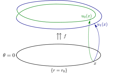
Figure 6: This very rough scheme captures only the topological aspect of the situation to illustrate the fact that the image under the set-valued map $f$ of each circle $\{r=r_{0}\}$, $0<r_{0}<1$, is a twice-winding, non-self-intersecting cycle; on top of each point $x$ on the circle there are two points, $u_{0}(x)$ and $u_{1}(x)$. We have also marked the point corresponding to angle $\theta=0$ that is mapped to the interface between the parameterizations $u_{0}$ and $u_{1}$ of the image of $f$. More accurate depictions of the situation can be found in Figures 7–9.

Let

$$\Delta=\{(x,y)\in\Omega\times Y:|\langle y,u_{0}(x)\rangle|>\|x\|^{6}/10\}.$$ (49)

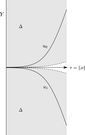
Figure 8: Radial scheme of the graph of $f$, made up of those of $u_{0}$ and $u_{1}$, and of $\Delta$ (shaded, with dashed boundary).

Note that $\|u_{i}(x)\|^{2}=\|x\|^{6}$, so the graph of $f$ is contained in $\Delta$; see Figures 7 and 8. Also, for each $0\neq x\in\Omega$, the set of points $y\in Y$ with $(x,y)\in\Delta$ has two connected components corresponding to the sign of the inner product $\langle y,u_{0}(x)\rangle$.

In order to define an auxiliary function $\psi\colon(\Omega\times Y)\setminus\{0\}\to[0,1]\in C^{\infty}$ that will be of great utility, pick a function $\rho\in C^{\infty}(\mathbb{R};[0,1])$ such that $\rho(r)=1$ for all $r\geq 1$ and $\rho(-r)=1-\rho(r)$, and let

$$\psi(x,y)=\rho\left(\frac{10\langle y,u_{0}(x)\rangle}{\|x\|^{6}}\right),\quad(x,y)\in\Omega\times Y.$$

Then

• $\psi(x,y)=1$ for $(x,y)\in\Delta$ with $\langle y,u_{0}(x)\rangle<0$, and

• $\psi(x,y)=0$ for $(x,y)\in\Delta$ with $\langle y,u_{0}(x)\rangle>0$.

For later use we record the following properties of $\psi$ (see Figure 7):

Lemma 3.3.

1. $|\psi(x,y)|\leq 1$.

2. the function

   $$U(x,y)=\begin{cases}\psi(x,y)u_{0}(x)+(1-\psi(x,y))u_{1}(x),&(x,y)\neq(0,0),\\ 0,&(x,y)=(0,0)\end{cases}$$

   is smooth on $(\Omega\setminus\{0\})\times Y$, and can be alternatively written as

   $$U(x,y)=\begin{cases}(2\psi(x,y)-1)u_{0}(x),&(x,y)\neq(0,0),\\ 0,&(x,y)=(0,0),\end{cases}$$

   because $u_{0}=-u_{1}$, and verifies

   $$\|U(x,y)\|=O(\|x\|^{3})$$

   as $x\to 0$.

3. On $\Delta$, the function $U(x,y)$ coincides either with $u_{0}(x)$ or with $u_{1}(x)$, whichever is closest to $y$.

4. For $i=0,1$, let $Du_{i}$ be the $2\times 2$ matrix

   $$Du_{i}=\left(\frac{\partial u_{i}}{\partial x_{1}},\frac{\partial u_{i}}{\partial x_{2}}\right),$$

   except at the points of the form $(a,0)$, $a\geq 0$, where this is not defined; we define $Du_{i}$ there by extending it continuously from above, namely,

   $$Du_{i}(a,0)\coloneqq(-1)^{i}a^{2}\begin{pmatrix}3&0\\ 0&1/2\end{pmatrix},\quad a\geq 0.$$

   The function

   $$V(x,y)=\begin{cases}\psi(x,y)Du_{0}(x)+(1-\psi(x,y))Du_{1}(x),&(x,y)\neq(0,0),\\ 0,&(x,y)=(0,0),\end{cases}$$

   is smooth on $(\Omega\setminus\{0\})\times Y$, and

   $$\|V(x,y)\|=O(\|x\|^{2})$$

   as $x\to 0$.

5. On $\Delta$, the function $V(x,y)$ coincides either with $Du_{0}(x)$ or with $Du_{1}(x)$, according to whether $u_{0}(x)$ or $u_{1}(x)$ is closest to $y$, respectively.

Proof.

Using Lemma 3.4 below with $u=u_{0}$ and then again with $u=Du_{0}$, we see that $U(x,y)=(2\psi(x,y)-1)u_{0}(x)$ and $V(x,y)=(2\psi(x,y)-1)Du_{0}(x)$ are smooth on $(\Omega\setminus\{0\})\times Y$. The rest of the lemma is clear from the definitions. ∎

Lemma 3.4.

Let $k>0$ and let $u\colon\Omega\setminus\{(a,0):a\geq 0\}\to\mathbb{R}^{k}$ be a smooth function such that, for all derivatives $\partial^{I}u$ of $u$, of any order including zero, we have that the following limits exist and satisfy

$$\lim_{\begin{subarray}{c}\bar{a}\to a\\ b\searrow 0\end{subarray}}\partial^{I}u(\bar{a},b)=-\lim_{\begin{subarray}{c}\bar{a}\to a\\ b\nearrow 0\end{subarray}}\partial^{I}u(\bar{a},b),\quad a>0.$$

Assume additionally that

$$u(a,0)=\lim_{b\searrow 0}u(a,b),\quad a>0.$$ (50)

Then $(2\psi(x,y)-1)u(x)$ is $C^{\infty}$ on $(\Omega\setminus\{0\})\times Y$.

Proof.

Fix $y\in Y$ and $a>0$. Take sequences $(a_{i})\subset\mathbb{R}$, $(b_{i})\subset\mathbb{R}_{>0}$, $(y_{i})\subset\mathbb{R}^{2}$ such that $a_{i}\to a$, $b_{i}\searrow 0$, $y_{i}\to y$. We have, using $\rho(r)=1-\rho(-r)$, for every multi-index $I$, and every $a>0$ and $y\in Y$,

$$\lim_{\begin{subarray}{c}\bar{a}\to a\\ b\searrow 0\\ \bar{y}\to y\end{subarray}}\partial^{I}[(2\psi((\bar{a},b),\bar{y})-1)u(\bar{a},b)] =\lim_{i\to+\infty}\partial^{I}[(2\psi((a_{i},b_{i}),y_{i})-1)u(a_{i},b_{i})]$$

$$=\lim_{i\to+\infty}\partial^{I}[(2\rho\left(\frac{10\langle y_{i},u_{0}(a_{i},b_{i})\rangle}{\|(a_{i},b_{i})\|^{6}}\right)-1)u(a_{i},b_{i})]$$

$$=\lim_{i\to+\infty}\partial^{I}[(2(1-\rho\left(-\frac{10\langle y_{i},u_{0}(a_{i},b_{i})\rangle}{\|(a_{i},b_{i})\|^{6}}\right))-1)u(a_{i},b_{i})]$$

$$=\lim_{i\to+\infty}\partial^{I}[(2(1-\rho\left(\frac{10\langle y_{i},-u_{0}(a_{i},b_{i})\rangle}{\|(a_{i},b_{i})\|^{6}}\right))-1)u(a_{i},b_{i})]$$

$$=\lim_{i\to+\infty}\partial^{I}[(2(1-\rho\left(\frac{10\langle y_{i},u_{0}(a_{i},-b_{i})\rangle}{\|(a_{i},b_{i})\|^{6}}\right))-1)u(a_{i},b_{i})]$$

$$=\lim_{i\to+\infty}\partial^{I}[-(2\rho\left(\frac{10\langle y_{i},u_{0}(a_{i},-b_{i})\rangle}{\|(a_{i},b_{i})\|^{6}}\right)-1)u(a_{i},b_{i})]$$

$$=\lim_{i\to+\infty}\partial^{I}[(2\rho\left(\frac{10\langle y_{i},u_{0}(a_{i},-b_{i})\rangle}{\|(a_{i},-b_{i})\|^{6}}\right)-1)u(a_{i},-b_{i})]$$

$$=\lim_{i\to+\infty}\partial^{I}[(2\psi((a_{i},-b_{i}),y_{i})-1)u(a_{i},-b_{i})]$$

$$=\lim_{\begin{subarray}{c}\bar{a}\to a\\ b\nearrow 0\\ \bar{y}\to y\end{subarray}}\partial^{I}[(2\psi((\bar{a},b),\bar{y})-1)u(\bar{a},b)]$$

This means that all derivatives of $(2\psi(x,y)-1)u(x)$ exist on $\{(a,0):a>0\}$. A similar calculation, together with (50), shows that $(2\psi(x,y)-1)u(x)$ is continuous. This shows that $(2\psi(x,y)-1)u(x)$ is $C^{\infty}$ on $(\Omega\setminus\{0\})\times Y$, as the continuity of the partial derivatives near a given point implies their existence at the point. ∎

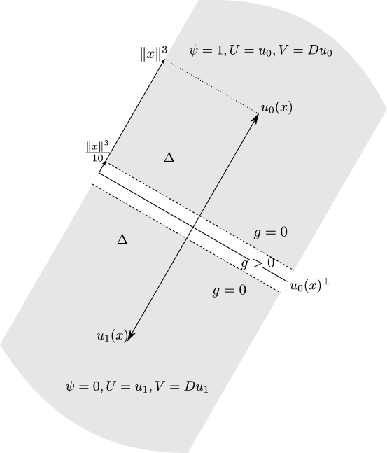
Figure 7: For $x\in\Omega$, this is the plane $\{x\}\times Y$. We have shaded the region $\Delta$, and indicated the vectors $u_{0}(x)$ and $u_{1}(x)=-u_{0}(x)$, together with their length, $\|x\|^{3}$, and the distance from $\Delta$ to the origin, $\|x\|^{3}/10$. We have also indicated what the values of $\psi$, $U$, and $V$ are on each of the connected components of $\Delta\cap(\{x\}\times Y)$. We have also included a reminder that $g$ (defined just after Lemma 3.3) is positive only outside of $\Delta$.

Take also a positive function $g\colon\Omega\times Y\to\mathbb{R}$ that will be auxiliary at helping us force minimizers of the proposed Lagrangian $L$ (to be defined below) to be supported in $\Delta$. We take $g$ such that

• $g\in C^{\infty}(\Omega\times Y)$,

• $g(x,y)\geq 0$,

• $g(x,y)=0$ for all $(x,y)\in\Delta$, and

• $g$ verifies

  $$\|y-U(x,y)\|^{2}+g(x,y)\geq\min_{i\in\{0,1\}}\|y-u_{i}(x)\|^{2}$$ (51)

  if $(x,y)\notin\Delta$.

  Observe that, by Lemma 3.3(ii)–(iii), the function

  $$S(x,y)\coloneqq\min_{i}\|y-u_{i}(x)\|^{2}-\|y-U(x,y)\|^{2}$$

  vanishes on $\Delta$ and is smooth everywhere except at the locus of points of the form $(x,0)$ (i.e., $y=0$), $x\in\Omega$, since it is there that $\|y-u_{0}(x)\|=\|u_{0}(x)\|=\|u_{1}(x)\|=\|y-u_{1}(x)\|$. Also, by Lemma 3.3(ii), $S(x,y)=O(\|x\|^{3})$ as $x\to 0$. Thus in order to get a function $g$ that complies with inequality (51), it suffices to take $g$ equal to $S$ in a small neighborhood of $\Delta$ while ensuring that it remains $\geq S$ everywhere.

The function $g$ will force the minimizers to be supported within $\Delta$. Remark that $g(0,0)=0$ because $g$ is $C^{\infty}$, $g$ vanishes on $\Delta$, and $(0,0)\in\overline{\Delta}$.

Now we can define $L\colon\Omega\times Y\times Z\to\mathbb{R}$ to be given by

$$L(x,y,z)=\|y-U(x,y)\|^{2}+\|z-V(x,y)\|^{2}+g(x,y);$$ (52)

in other words,

$$L(x,y,z)=\|y-\psi(x,y)u_{0}(x)-(1-\psi(x,y))u_{1}(x)\|^{2}\\ +\|z-\psi(x,y)Du_{0}(x)-(1-\psi(x,y))Du_{1}(x)\|^{2}+g(x,y),$$

for $(0,0)\neq(x,y)\in\Omega\times Y$, and $z\in Z$, and

$$L(0,0,z)=\|z\|^{2},\quad z\in Z.$$

Observe that on $(x,y)\in\Delta$ the expression (52) simplifies to

$$L(x,y,z)=\|y-u_{i}(x)\|^{2}+\|z-Du_{i}(x)\|^{2}\quad\textrm{if}\quad i=\operatornamewithlimits{arg\,min}_{j\in\{0,1\}}\|y-u_{j}(x)\|^{2}$$ (53)

because $g$ vanishes on $\Delta$ and because of Lemma 3.3.

Lemma 3.5.

$L$ is of class $C^{1,1}_{\mathrm{loc}}$.

Proof of Lemma 3.5.

From Lemma 3.3, we know that $U$ and $V$ are $C^{\infty}$ on $(\Omega\setminus\{0\})\times Y$. This, together with the expression (52) defining $L$ away from the origin, and the smoothness of $g$, we conclude that $L$ is $C^{\infty}$ on $(\Omega\setminus\{0\})\times Y$. For fixed $y^{\prime}\in Y$ and $z^{\prime}\in Z$, as $(x,y,z)\to(0,y^{\prime},z^{\prime})$, using the estimates from Lemma 3.3 as well as the fact that

$$g(x,y)=\begin{cases}O(\|x\|^{2}+\|y\|^{2}),&y^{\prime}\neq 0,\\ 0&y^{\prime}=0,\end{cases}$$

as $(x,y)\to(0,y^{\prime})$ (which follows from $g$ being smooth, nonnegative, and vanishing at the origin, $g(0,0)=0$, because then necessarily $\nabla g(0,0)=0$; and from $g(x,y)=0$ on a neighborhood of every point $(0,y)$, $y\neq 0$, as this point belongs to $\Delta$), we have

$$|L(x,y,z) -L(0,y^{\prime},z^{\prime})-2\langle y^{\prime},y-y^{\prime}\rangle-2\langle z^{\prime},z-z^{\prime}\rangle|$$

$$=|\|y-U(x,y)\|^{2}+\|z-V(x,y)\|^{2}+g(x,y)$$

$$\qquad-\|y^{\prime}\|^{2}-\|z^{\prime}\|^{2}-2\langle y^{\prime},y-y^{\prime}\rangle-2\langle z^{\prime},z-z^{\prime}\rangle|$$

$$=|\|y\|^{2}-\|y^{\prime}\|^{2}-2\langle y^{\prime},y-y^{\prime}\rangle$$

$$\qquad+\|U(x,y)\|^{2}-2\langle y,U(x,y)\rangle$$

$$\qquad\|V(x,y)\|^{2}-2\langle z,V(x,y)\rangle+g(x,y)$$

$$\qquad\|z\|^{2}-\|z^{\prime}\|^{2}-2\langle z^{\prime},z-z^{\prime}\rangle|$$

$$\leq\|y^{2}-y^{\prime}\|^{2}+\|y^{2}-y^{\prime}\|^{2}+O(\|x\|^{6}+\|y\|\|x\|^{3}$$

$$\qquad+\|x\|^{4}+\|z\|\|x\|^{2}+\chi_{y^{\prime}\neq 0}(\|x\|^{2}+\|y\|^{2}))$$

$$\qquad+\|z-z^{\prime}\|^{2}$$

$$\leq O(\|x\|^{2}+\|y-y^{\prime}\|^{2}+\|z-z^{\prime}\|^{2})$$

$$=O(\|(x,y,z)-(0,y^{\prime},z^{\prime})\|^{2}).$$

Here, $\chi_{y^{\prime}\neq 0}\in\{0,1\}$ vanishes when $y^{\prime}=0$ and is 1 otherwise. Then [7, Proposition 4.11.3] implies that the derivative is locally Lipschitz continuous. ∎

Proof of the theorem.

We present the proof in several steps.

Step 1. $\displaystyle\min_{(\mu,\mu_{\partial})\in\mathcal{M}}\int_{\Omega\times Y\times Z}L\,d\mu=0.$

The map $f$ can be encoded using the measure $\mu$ on $\Omega\times Y\times Z$ defined by the pushforwards

$$\mu=\tfrac{1}{2}\xi_{0\#}dx+\tfrac{1}{2}\xi_{1\#}dx$$

where $dx$ is Lebesgue measure on $\Omega$, and $\xi_{i}\colon\Omega\to\Omega\times Y\times Z$ is the map

$$\xi_{i}(x)=(x,u_{i}(x),Du_{i}(x)),\quad x\in\Omega.$$

By the definition (49) of $\Delta$, it holds that $(x,u_{i}(x))\in\Delta$ for $i\in\{1,2\}$. Therefore the $(x,y)$-marginal of $\mu$ is supported in $\Delta$, where $L$ is given by (53) (see also Figure 7). It follows that

$$\int_{\Omega\times Y\times Z}L\,d\mu=\int_{\Delta\times Z}L\,d\mu =\frac{1}{2}\sum_{i=0}^{1}\int_{\Omega}L(x,u_{i}(x),Du_{i}(x))\,dx$$

$$=\frac{1}{2}\sum_{i=0}^{1}\int_{\Omega}\|u_{i}(x)-u_{i}(x)\|^{2}+\|Du_{i}(x)-Du_{i}(x)\|^{2}\,dx=0,$$

Since the integrand is nonnegative, this is the minimum of the integral of $L$ over any measure $\mu$ with $(\mu,\mu_{\partial})\in\mathcal{M}$.

Step 2. Reparameterization of $f$ using $\bar{u}_{\alpha}$ and choice of $\alpha_{0}$.

For $\alpha\in\mathbb{R}$, let $\bar{u}_{\alpha}$ the $\mathbb{R}^{2}$-valued function on $\Omega$ given by

$$\bar{u}_{\alpha}(r(\cos(\theta+\alpha),\sin(\theta+\alpha)))=r^{3}\left(\cos\frac{\theta+\alpha}{2},\sin\frac{\theta+\alpha}{2}\right),\quad r\in[0,1),\,\theta\in[0,2\pi),$$ (54)

so that $\bar{u}_{\alpha}=-\bar{u}_{\alpha+2\pi}$. Thus if $\alpha\in[0,2\pi)$ then

$$\bar{u}_{\alpha}(x)=\begin{cases}u_{0}(x),&\textrm{for $\theta(x)\in[\alpha,2\pi)$},\\ u_{1}(x),&\textrm{for $\theta(x)\in[0,\alpha)$},\end{cases}\quad\bar{u}_{\alpha+2\pi}(x)=\begin{cases}u_{1}(x),&\textrm{for $\theta(x)\in[\alpha,2\pi)$},\\ u_{0}(x),&\textrm{for $\theta(x)\in[0,\alpha)$},\end{cases}$$ (55)

where $x\in\Omega$ and $\theta(x)\in[0,2\pi)$ is the polar angle of $x=r(\cos\theta(x),\sin\theta(x))$. Therefore $u_{0}=\bar{u}_{0}$ and $u_{1}=\bar{u}_{2\pi}$. Just like $u_{0}$ and $u_{1}$ parameterize the image of $f$ and the jump between the two happens at angle 0 (see Figure 6), for each $\alpha\in\mathbb{R}$ the functions $\bar{u}_{\alpha}$ and $\bar{u}_{\alpha+2\pi}=-\bar{u}_{\alpha}$ give another parametrization of the image of $f$, with the jump from one chart $u_{1}$ to the other $u_{0}$ at angle $\alpha$.

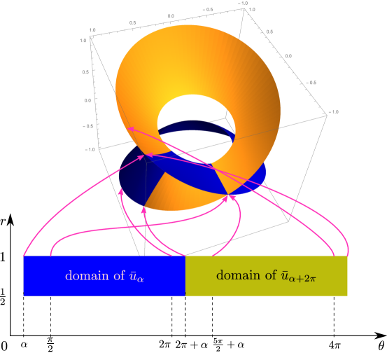
Figure 9: This 3-dimensional projection of the graph of $f|_{\Gamma}$ under the map $(x_{1},x_{2},y_{1},y_{2})\mapsto(x_{1},x_{2},y_{1})$ has been colored to distinguish the images of $u_{\alpha}$ and $u_{\alpha+2\pi}$. We have also represented the domains, in polar coordinates, of these functions, and indicated where some points are mapped. Note that the apparent self-intersection is an artifact of the projection that does not occur in reality.

Let $\Gamma\subset\Omega$ be the corona consisting of points $x$ with radius $\frac{1}{2}\leq|x|\leq 1$, whose area is $|\Gamma|=3\pi/4$. Take

$$E=\frac{1}{41}.$$

Let $h\colon\Omega\to Y$ be any function of class $W^{1,2}(\Omega)$, a candidate solution to the optimization problem on the left-hand side of (47).

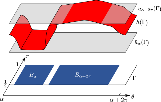
Figure 10: In polar coordinates $(\theta,r)$, the corona $\Gamma$ can be parameterized by the rectangle $[\alpha,\alpha+2\pi]\times[\tfrac{1}{2},1]$, and its image under $\bar{u}_{\alpha}$ and $\bar{u}_{\alpha+2\pi}$ is a double-covering. In the picture, we illustrate the definition of the disjoint sets $B_{\alpha}$ and $B_{\alpha+2\pi}$ for a given function $h$; these sets are the subsets of $\Gamma$ in which $h$ is $E$-close to $\bar{u}_{\alpha}(\Gamma)$ and $\bar{u}_{\alpha+2\pi}(\Gamma)$, respectively. Changing $\alpha$ translates the picture in the $\theta$ direction. While $h$ is $2\pi$-periodic in $\theta$, the overall picture is $4\pi$-periodic because the right-hand border $\bar{u}_{\alpha}(\{\alpha+2\pi\}\times[\tfrac{1}{2},1])$ coincides with the left-hand border $\bar{u}_{\alpha+2\pi}(\{\alpha\}\times[\tfrac{1}{2},1])$, and similarly for $\bar{u}_{\alpha+2\pi}(\{\alpha+2\pi\}\times[\tfrac{1}{2},1])$ and $\bar{u}_{\alpha}(\{\alpha\}\times[\tfrac{1}{2},1])$. As we move $\alpha$, the union $B_{\alpha}\cup B_{\alpha+2\pi}$ does not change, but the contents of the sets $B_{\alpha}$ and $B_{\alpha+2\pi}$ get gradually interchanged. Although we have drawn $h$, $B_{\alpha}$ and $B_{\alpha+2\pi}$ as independent of $r$, this need not be the case.

For $\alpha\in\mathbb{R}$, let $B_{\alpha}\subset\Omega$ be defined by

$$B_{\alpha}=\{x\in\Gamma\,:\,\|h(x)-\bar{u}_{\alpha}(x)\|\leq E\},$$

(see Figure 10). Given $\alpha$, the union $B_{\alpha}\cup B_{\alpha+2\pi}$ is, because of (55), the set of points $x\in\Gamma$ such that $h(x)$ is $E$-close to $f(x)$. As the angle $\alpha$ that determines which of those points are in $B_{\alpha}$ and which are in $B_{\alpha+2\pi}$ varies, the areas of these sets vary continuously; in other words, $\alpha\mapsto|B_{\alpha}|$ is continuous. Let

$$\varphi(\alpha)=|B_{\alpha}|-|B_{\alpha+2\pi}|.$$

Then $\varphi$ is continuous, verifies $\varphi(\alpha)=-\varphi(\alpha+2\pi)$, and is $4\pi$-periodic in $\alpha$. By the intermediate value theorem, there is some $\alpha_{0}\in[0,2\pi)$ such that $\varphi(\alpha_{0})=0$. In particular, with our choice of $\alpha_{0}$ we have

$$|B_{\alpha_{0}}|=|B_{{\alpha_{0}}+2\pi}|=\frac{|B_{\alpha_{0}}|+|B_{{\alpha_{0}}+2\pi}|}{2}.$$

Step 3. Bound for $h$ when $|B_{\alpha_{0}}|=|B_{{\alpha_{0}}+2\pi}|<|\Gamma|/4$.

Let $j(x)\in\{0,1\}$ be given by

$$j(x)=\operatornamewithlimits{arg\,min}_{j\in\{0,1\}}\|h(x)-\bar{u}_{{\alpha_{0}}+2\pi j}(x)\|,\quad x\in\Gamma.$$

We have, from (51) and (55),

$$\|h(x)-U(x,h(x))\|^{2}+g(x,y)\geq\|h(x)-\bar{u}_{{\alpha_{0}}+2\pi j(x)}(x)\|^{2}.$$

We use this to get the uniform bound

$$\int_{\Omega}L(x,h(x),Dh(x))dx =\int_{\Omega}\|h(x)-U(x,h(x))\|^{2}$$

$$\qquad+\|Dh(x)-V(x,h(x))\|^{2}+g(x,y)\,dx$$

$$\geq\int_{\Gamma}\|h(x)-U(x,h(x))\|^{2}+g(x,y)\,dx$$

$$\geq\int_{\Gamma}\|h(x)-\bar{u}_{{\alpha_{0}}+2\pi j(x)}(x)\|^{2}dx$$

$$\geq\int_{\Gamma\setminus(B_{\alpha_{0}}\cup B_{\alpha_{0}+2\pi})}E^{2}\,dx$$

$$\geq E^{2}(|\Gamma|-|B_{\alpha_{0}}|-|B_{{\alpha_{0}}+2\pi}|)$$

$$=E^{2}\left(|\Gamma|-2\frac{|\Gamma|}{4}\right)=E^{2}\frac{|\Gamma|}{2}>0.$$

We have additionally used the fact that, by our choice of the sets $B_{\alpha_{0}}$ and $B_{\alpha_{0}+2\pi}$, for $x$ in these sets it holds that $\|h(x)-\bar{u}_{\alpha_{0}+2\pi j(x)}(x)\|\geq E$.

Step 4. Definition and properties of $\bar{h}_{0}$.

Let, for $x\in\Gamma$,

$$\bar{h}_{0}(x)=\min\left(\|h(x)-\bar{u}_{{\alpha_{0}}}(x)\|,\;\frac{1}{10}\right).$$

The role of the function $\bar{h}_{0}$ is to give a sort of truncated version of the distance from $h$ to $\bar{u}_{{\alpha_{0}}}$ that will be useful in our estimation below. Note that, by the definition of $B_{\alpha_{0}}$, $\bar{h}_{0}(x)\leq E$ on $B_{\alpha_{0}}$.

Observe that if we parameterize $\Gamma$ in polar coordinates with the rectangle $[\frac{1}{2},1]\times[\alpha_{0},\alpha_{0}+2\pi)$, then $\bar{u}_{\alpha}$ is smooth on that chart, and $\bar{h}_{0}$ is in $W^{1,2}$, as is $h$. In other words, although $\bar{h}_{0}$ is possibly discontinuous on the ray segment

$$R_{\alpha_{0}}=\{x\in\Gamma:x=r(\cos{\alpha_{0}},\sin{\alpha_{0}}),\;r\in[\frac{1}{2},1]\}$$

corresponding to angle $\alpha_{0}$, it is a Sobolev $W^{1,2}$ function on the rest of $\Gamma$.

Claim. We have, for almost every $x\in\Gamma\setminus R_{\alpha_{0}}$,

$$\|Dh(x)-V(x,h(x))\|\geq\|D\bar{h}_{0}(x)\|.$$ (56)

Proof of the claim..

We have the following cases for $x\in\Gamma\setminus R_{\alpha_{0}}$:

• In the region where $\|h(x)-\bar{u}_{{\alpha_{0}}}(x)\|\geq 1/10$, the function $\bar{h}_{0}$ is constant so the right-hand side equals zero, and the inequality is verified trivially.

• In the region where $0<\|h(x)-\bar{u}_{{\alpha_{0}}}(x)\|<1/10$, we have $(x,h(x))\in\Delta$ because for $x\in\Gamma$ we have $\frac{1}{2}\leq\|x\|\leq 1$ and then, expanding the squared inequality

  $$0<\|h(x)-\bar{u}_{{\alpha_{0}}}(x)\|^{2}=\|h(x)\|^{2}-2\langle\bar{u}_{{\alpha_{0}}}(x),h(x)\rangle+\|\bar{u}_{{\alpha_{0}}}(x)\|^{2}<\tfrac{1}{10^{2}},$$

  we get

  $$\langle\bar{u}_{\alpha_{0}}(x),h(x)\rangle>\tfrac{1}{2}(\|h(x)\|^{2}+\|\bar{u}_{\alpha_{0}}(x)\|^{2}-\tfrac{1}{10^{2}})\\ \geq\tfrac{1}{2}((\|\bar{u}_{\alpha_{0}}(x)\|-\tfrac{1}{10})^{2}+\|\bar{u}_{\alpha_{0}}(x)\|^{2}-\tfrac{1}{10^{2}})=\|\bar{u}_{\alpha_{0}}(x)\|^{2}-\tfrac{1}{10}\|\bar{u}_{\alpha_{0}}(x)\|\\ =\|x\|^{6}-\tfrac{1}{10}\|x\|^{3}>\frac{\|x\|^{6}}{10}.$$

  Since the left-hand side equals $|\langle u_{i}(x),h(x)\rangle|$ for some $i=0,1$ by (55), this shows that $(x,h(x))\in\Delta$, as per its definition (49). This, in turn, means (by Lemma 3.3(iv)) that the left-hand side of (56) reduces to

  $$\|Dh(x)-D\bar{u}_{\alpha_{0}}(x)\|$$

  by our choice of $\psi$ and (55). Inequality (56) then follows by taking $\phi(x)=h(x)-\bar{u}_{\alpha_{0}}(x)$ and observing that all weakly differentiable functions $\phi$ verify, almost everywhere within the set where $\|\phi\|\neq 0$,

  $$\Big{\|}D\|\phi\|\Big{\|}=\left\|\frac{\phi}{\|\phi\|}D\phi\right\|=\left\|(D\phi)^{t}\frac{\phi^{t}}{\|\phi\|}\right\|\leq\|(D\phi)^{t}\|\frac{\|\phi\|}{\|\phi\|}=\|D\phi\|,$$

  where $(D\phi)^{t}$ is the transposed Jacobian matrix and $\|(D\phi)^{t}\|=\|D\phi\|$ is its operator norm.

• In the region where $\bar{h}_{0}(x)=\|h(x)-\bar{u}_{{\alpha_{0}}}(x)\|=0$, either the weak derivative of $\bar{h}_{0}$ vanishes wherever it is defined (because $\bar{h}_{0}$ is nonnegative), hence verifying (56); the set where it is not defined has measure zero because $\bar{h}_{0}$ is weakly differentiable since $h$ is.

∎

Step 5. Bound for $h$ when

$$|B_{\alpha_{0}}|=|B_{{\alpha_{0}}+2\pi}|\geq\frac{|\Gamma|}{4}.$$ (57)

For $x\in B_{\alpha_{0}+2\pi}$, $\|h(x)-\bar{u}_{\alpha_{0}+2\pi}\|\leq E$, so

$$\|\bar{u}_{\alpha_{0}}(x)-\bar{u}_{\alpha_{0}+2\pi}(x)\|\leq\|\bar{u}_{\alpha_{0}}(x)-h(x)\|+\|h(x)-\bar{u}_{\alpha_{0}+2\pi}(x)\|\leq\|\bar{u}_{\alpha_{0}}(x)-h(x)\|+E,$$

and then

$$\bar{h}_{0}(x)=\|h(x)-\bar{u}_{\alpha_{0}}(x)\|>\|u_{\alpha_{0}}(x)-\bar{u}_{\alpha_{0}+2\pi}(x)\|-E\geq\frac{1}{8}-E>\frac{1}{10}.$$

Hence, using (57),

$$M\coloneqq|\Gamma|^{-1}\int_{\Gamma}\bar{h}_{0}(x)dx\geq|\Gamma|^{-1}\int_{B_{\alpha_{0}+2\pi}}\frac{1}{10}dx\geq\frac{|B_{\alpha_{0}+2\pi}|}{10|\Gamma|}\geq\frac{1}{40}.$$

The domain consisting of the slit corona $\Gamma\setminus R_{\alpha_{0}}$ satisfies the so-called cone property [8, Definition 2.5.14]. By (56) together with the Poincaré-Wirtinger inequality [8, Theorem 2.5.21] for the domain $\Gamma\setminus R_{\alpha_{0}}$ with constant $C>0$,

$$\int_{\Omega}L(x,h(x),Dh(x))dx =\int_{\Omega}\|h(x)-U(x,h(x)\|^{2}$$

$$\qquad+\|Dh(x)-V(x,h(x))\|^{2}+g(x,y)\,dx$$

$$\geq\int_{\Gamma}\|Dh(x)-V(x,h(x))\|^{2}dx$$

$$\geq\int_{\Gamma\setminus R_{\alpha_{0}}}\|D\bar{h}_{0}(x)\|^{2}dx$$

$$\geq C\int_{\Gamma\setminus R_{\alpha_{0}}}\left|\bar{h}_{0}(x)-M\right|^{2}dx.$$

Now, since for $x\in B_{\alpha_{0}}$ we have $0\leq\bar{h}_{0}(x)\leq E=1/41<1/{40}\leq M$ there, we have

$$|\bar{h}_{0}(x)-M|\geq F\coloneqq\frac{1}{40}-\frac{1}{41}>0,$$

so the above is

$$C\int_{\Gamma\setminus R_{\alpha_{0}}}\left|\bar{h}_{0}(x)-M\right|^{2}dx\geq C\int_{B_{\alpha_{0}}}F^{2}dx=CF^{2}|B_{\alpha_{0}}|\geq CF^{2}\frac{|\Gamma|}{4}>0.$$

This is a uniform lower bound for all $h\in W^{1,2}(\Omega)$ satisfying the above constraints.

Together, the bounds from Steps 3 and 5 prove the theorem. ∎

4 Positive gap with integral constraints

The reader may be curious why we have not included, in the statements of Theorems 2.3 and 2.4 and in the definitions (6) and (10) of $M_{\mathrm{c}}$ and $M_{\mathrm{r}}$, any integral constraints of the form

$$\int_{\Omega}H(x,y(x),Dy(x))\,dx\leq 0\quad\textrm{or}\quad\int_{\Omega}H(x,y(x),Dy(x))\,dx=0.$$

The reason is that in the presence of these constraints, there may be a gap between the classical case and its relaxation. The following two sections give examples of such situations. The idea for each of these examples works in any dimensions $n,m>0$, and we show them in the special case $n=m=1$ for simplicity.

We use the same notations as in the definitions 6 and 10 of $M_{\mathrm{c}}$ and $M_{\mathrm{r}}$.

4.1 Inequality integral constraints

Let $\Omega=(0,1)\subset\mathbb{R}$, $Y=\mathbb{R}$, $L(x,y,z)=y$, $F(x,y,z)=y(1-y)$, $F_{\partial}=G=G_{\partial}=0$. Note that the only Lipschitz curves $y\colon\Omega\to Y$ such that $F(x,y(x),Dy(x))=0$ are $y_{0}(x)=0$ and $y_{1}(x)=1$, $x\in\Omega$, and these satisfy

$$\int_{\Omega}L(x,y_{0}(x),Dy_{0}(x))dx=\int_{0}^{1}0\,dx=0\quad\textrm{and}\quad\int_{\Omega}L(x,y_{1}(x),Dy_{1}(x))dx=\int_{0}^{1}1\,dx=1.$$

Let $H(x,y,z)=1-10y$. Consider the problem of computing $M_{\mathrm{c}}$ and $M_{\mathrm{r}}$ as in 6 and 10, above, with the additional integral constraints

$$\int_{\Omega}H(x,y(x),Dy(x))\,dx\leq 0\quad\textrm{and}\quad\int_{\Omega\times Y\times Z}H(x,y,z)\,d\mu(x,y,z)\leq 0,$$

to be satisfied by the respective competitors $y$ and $(\mu,\mu_{\partial})$. We will show that in this case $M_{\mathrm{c}}>M_{\mathrm{r}}$.

For the classical case, we have

$$\int_{\Omega}H(x,y_{0},Dy_{0})\,dx=\int_{0}^{1}1-0\,dx=1\stackrel{{\scriptstyle!}}{{>}}0\quad\textrm{and}\quad\int_{\Omega}H(x,y_{1},Dy_{1})\,dx=\int_{0}^{1}1-10\,dx=-9\leq 0,$$

so in the calculation of $M_{\mathrm{c}}$ the only competitor is $y_{1}$, because $y_{0}$ does not satisfy the integral constraint. We conclude that $M_{\mathrm{c}}=1$.

For the relaxed case, consider the measure $\mu=\frac{9}{10}\mu_{0}+\frac{1}{10}\mu_{1}$, where $\mu_{i}$ is the measure induced by $y_{i}$, $i=0,1$. Then

$$\int_{\Omega\times Y\times Z}H\,d\mu=\tfrac{9}{10}\int_{\Omega\times Y\times Z}H\,d\mu_{0}+\tfrac{1}{10}\int_{\Omega\times Y\times Z}H\,d\mu_{1}=\tfrac{9}{10}-9\tfrac{1}{10}=0,$$

so $\mu$ satisfies the constraint. We also have

$$\int_{\Omega\times Y\times Z}L\,d\mu=\tfrac{9}{10}\int_{\Omega\times Y\times Z}L\,d\mu_{0}+\tfrac{1}{10}\int_{\Omega\times Y\times Z}L\,d\mu_{1}=\tfrac{1}{10}.$$

Thus $M_{\mathrm{r}}\leq\frac{1}{10}<1=M_{\mathrm{c}}$.

4.2 Equality integral constraints

Let $\Omega=(0,1)\subset\mathbb{R}$, $Y=\mathbb{R}$, $L(x,y,z)=y$, $F(x,y,z)=y(y-1)(y-2)$, $F_{\partial}=G=G_{\partial}=0$. Note that the only Lipschitz curves $y\colon\Omega\to Y$ such that $F(x,y(x),Dy(x))=0$ are $y_{0}(x)=0$, $y_{1}(x)=1$, and $y_{2}(x)=2$, $x\in\Omega$, and these satisfy

$$\int_{\Omega}L(x,y_{i}(x),Dy_{i}(x))dx=\int_{0}^{1}i\,dx=i,\quad i=0,1,2.$$

Let $H(x,y,z)=\frac{7}{4}y-\frac{3}{4}y^{2}$. Consider the problem of computing $M_{\mathrm{c}}$ and $M_{\mathrm{r}}$ as in 6 and 10, above, with the additional integral constraints

$$\int_{\Omega}H(x,y(x),Dy(x))\,dx=\tfrac{1}{2}\quad\textrm{and}\quad\int_{\Omega\times Y\times Z}H(x,y,z)\,d\mu(x,y,z)=\tfrac{1}{2},$$

to be satisfied by the respective competitors $y$ and $(\mu,\mu_{\partial})$. We will show that in this case $M_{\mathrm{c}}>M_{\mathrm{r}}$ too.

For the classical case, we have

$$\int_{\Omega}H(x,y_{0},Dy_{0})\,dx=\int_{0}^{1}0\,dx=0\stackrel{{\scriptstyle!}}{{\neq}}\tfrac{1}{2}\quad\textrm{and}\quad\int_{\Omega}H(x,y_{1},Dy_{1})\,dx=\int_{0}^{1}\tfrac{7}{4}-\tfrac{3}{4}\,dx=1\stackrel{{\scriptstyle!}}{{\neq}}\tfrac{1}{2},$$

and

$$\int_{\Omega}H(x,y_{2},Dy_{2})\,dx=\int_{0}^{1}2\tfrac{7}{4}-4\tfrac{3}{4}dx=\tfrac{1}{2},$$

so in the calculation of $M_{\mathrm{c}}$ the set of competitors contains only $y_{2}$. We conclude that

$$M_{\mathrm{c}}=\int_{0}^{1}L(x,y_{2}(x),Dy_{2}(x))\,dx=\int_{0}^{1}2\,dx=2.$$

For the relaxed case, consider the measure $\mu=\frac{1}{2}\mu_{0}+\frac{1}{2}\mu_{1}$, where $\mu_{i}$ is the measure induced by $y_{i}$, $i=0,1$. Then

$$\int_{\Omega\times Y\times Z}H\,d\mu=\tfrac{1}{2}\int_{\Omega\times Y\times Z}H\,d\mu_{0}+\tfrac{1}{2}\int_{\Omega\times Y\times Z}H\,d\mu_{1}=0\tfrac{1}{2}+1\tfrac{1}{2}=\tfrac{1}{2},$$

so $\mu$ satisfies the constraint. We also have

$$\int_{\Omega\times Y\times Z}L\,d\mu=\tfrac{1}{2}\int_{\Omega\times Y\times Z}L\,d\mu_{0}+\tfrac{1}{2}\int_{\Omega\times Y\times Z}L\,d\mu_{1}=\tfrac{1}{2}.$$

Thus $M_{\mathrm{r}}\leq\frac{1}{2}<2=M_{\mathrm{c}}$.

5 Acknowledgements

This work has been supported by the Czech Science Foundation (GACR) under contract No. 20-11626Y, the European Union’s Horizon 2020 research and innovation programme under the Marie Skłodowska-Curie Actions, grant agreement 813211 (POEMA), by the AI Interdisciplinary Institute ANITI funding, through the French “Investing for the Future PIA3” program under the Grant agreement n^∘ ANR-19-PI3A-0004 as well as by the National Research Foundation, Prime Minister’s Office, Singapore under its Campus for Research Excellence and Technological Enterprise (CREATE) programme.

The authors would like to thank to Martin Kružík, Jared Miller, Corbinian Schlosser and Ian Tobasco for constructive feedback on this work.

Data availability statement.

This manuscript has no associated data.

Competing interests.

The authors have no competing interests.

References

- [1] Giovanni Alberti and Annalisa Massaccesi. On some geometric properties of currents and frobenius theorem. Rendiconti Lincei-Matematica e Applicazioni, 28(4):861–869, 2017.
- [2] Luigi Ambrosio. Transport equation and cauchy problem for non-smooth vector fields. In Calculus of variations and nonlinear partial differential equations, pages 1–41. Springer, 2008.
- [3] Patrick Bernard. Young measures, superposition and transport. Indiana Univ. Math. J., 57(1):247–275, 2008.
- [4] Alexander Chernyavsky, Jason J Bramburger, Giovanni Fantuzzi, and David Goluskin. Convex relaxations of integral variational problems: pointwise dual relaxation and sum-of-squares optimization. arXiv preprint arXiv:2110.03079, 2021.
- [5] Camillo De Lellis and Emanuele Spadaro. Regularity of area minimizing currents i: gradient l p estimates. Geometric and Functional Analysis, 24(6):1831–1884, 2014.
- [6] Lawrence C. Evans and Ronald F. Gariepy. Measure theory and fine properties of functions. CRC Press, 2015.
- [7] Albert Fathi. Weak kam theorem in lagrangian dynamics, preliminary version number 10. Available online, 2008.
- [8] L Gasinski and N Papageorgiou. Nonlinear analysis, volume 9 of ser. Math. Anal. Appl. Chapman & Hall/CRC, Boca Raton, FL, 2006.
- [9] R Hardt and J Pitts. Solving the plateau’s problem for hypersurfaces without the compactness theorem for integral currents. Geometric measure theory and the calculus of variations, 44:255–295, 1996.
- [10] Didier Henrion and Milan Korda. Convex computation of the region of attraction of polynomial control systems. IEEE Transactions on Automatic Control, 59(2):297–312, 2014.
- [11] Didier Henrion, Milan Korda, and Jean Bernard Lasserre. Moment-sos Hierarchy, The: Lectures In Probability, Statistics, Computational Geometry, Control And Nonlinear Pdes, volume 4. World Scientific, 2020.
- [12] Milan Korda, Didier Henrion, and Jean-Bernard Lasserre. Moments and convex optimization for analysis and control of nonlinear pdes. In E. Zuazua E. Trelat, editor, Handbook of Numerical Analysis, volume 23, chapter 10, pages 339–366. Elsevier, 2022.
- [13] Jean B Lasserre, Didier Henrion, Christophe Prieur, and Emmanuel Trélat. Nonlinear optimal control via occupation measures and LMI-relaxations. SIAM Journal on Control and Optimization, 47(4):1643–1666, 2008.
- [14] Jean Bernard Lasserre. Moments, positive polynomials and their applications, volume 1. World Scientific, 2009.
- [15] RM Lewis and RB Vinter. Relaxation of optimal control problems to equivalent convex programs. Journal of Mathematical Analysis and Applications, 74(2):475–493, 1980.
- [16] Francesco Maggi. Sets of finite perimeter and geometric variational problems: an introduction to Geometric Measure Theory. Number 135 in Cambridge studies in advanced mathematics. Cambridge University Press, 2012.
- [17] Swann Marx, Tillmann Weisser, Didier Henrion, and Jean Lasserre. A moment approach for entropy solutions to nonlinear hyperbolic pdes. Mathematical Control and Related Fields, 10(1):113–140, 2020.
- [18] Frank Morgan. Geometric measure theory: a beginner’s guide. Academic press, 2016.
- [19] JE Rubio. Generalized curves and extremal points. SIAM Journal on Control, 13(1):28–47, 1975.
- [20] JE Rubio. Extremal points and optimal control theory. Annali di Matematica Pura ed Applicata, 109(1):165–176, 1976.
- [21] Walter Rudin. Real and Complex Analysis. McGraw-Hill, 1968.
- [22] Andrea Schioppa. Unrectifiable normal currents in euclidean spaces. arXiv:1608.01635.
- [23] Emanuele Tasso. Decomposizione di correnti normali. Master’s thesis, University of Pisa, 5 2015.
- [24] Richard B Vinter and Richard M Lewis. The equivalence of strong and weak formulations for certain problems in optimal control. SIAM Journal on Control and Optimization, 16(4):546–570, 1978.
- [25] Laurence Chisholm Young. Lectures on the calculus of variations and optimal control theory. Saunders, Philadelphia, 1969.
- [26] Maciej Zworski. Decomposition of normal currents. Proceedings of the American Mathematical Society, 102(4):831–839, 1988.