Solving infinite-horizon POMDPs with memoryless
stochastic policies in state-action space

Abstract

Reward optimization in fully observable Markov decision processes is equivalent to a linear program over the polytope of state-action frequencies. Taking a similar perspective in the case of partially observable Markov decision processes with memoryless stochastic policies, the problem was recently formulated as the optimization of a linear objective subject to polynomial constraints. Based on this we present an approach for Reward Optimization in State-Action space (ROSA). We test this approach experimentally in maze navigation tasks. We find that ROSA is computationally efficient and can yield stability improvements over other existing methods.

Keywords:

POMDP, policy gradient, state-action frequencies, constrained optimization.

1 Introduction

Partially Observable Markov Decision Processes (POMDPs) offer a popular model for sequential decision making with state uncertainty. Here, actions are selected based on partial observations of the system’s state with the objective to maximize a cumulative discounted reward. We focus on infinite horizon problems and memoryless stochastic policies which offer an alternative to difficult-to-optimize policies based on belief states and policies with memory. Techniques such as policy iteration and value iteration usually require a belief state or a finite-state controller representation of the policy, and the standard approaches based on policy gradients [SMS⁺99, AYA18] can suffer from ill-conditioning when future rewards are not sufficiently discounted. Recently, a polynomial programming formulation of POMDPs was derived in [MM22], generalizing the linear program associated to MDPs. In this work we provide a practical implementation of this approach and demonstrate experimentally, in navigation problems of different sizes, that it offers a competitive alternative improving computational cost and numerical stability for a range of discount factors.

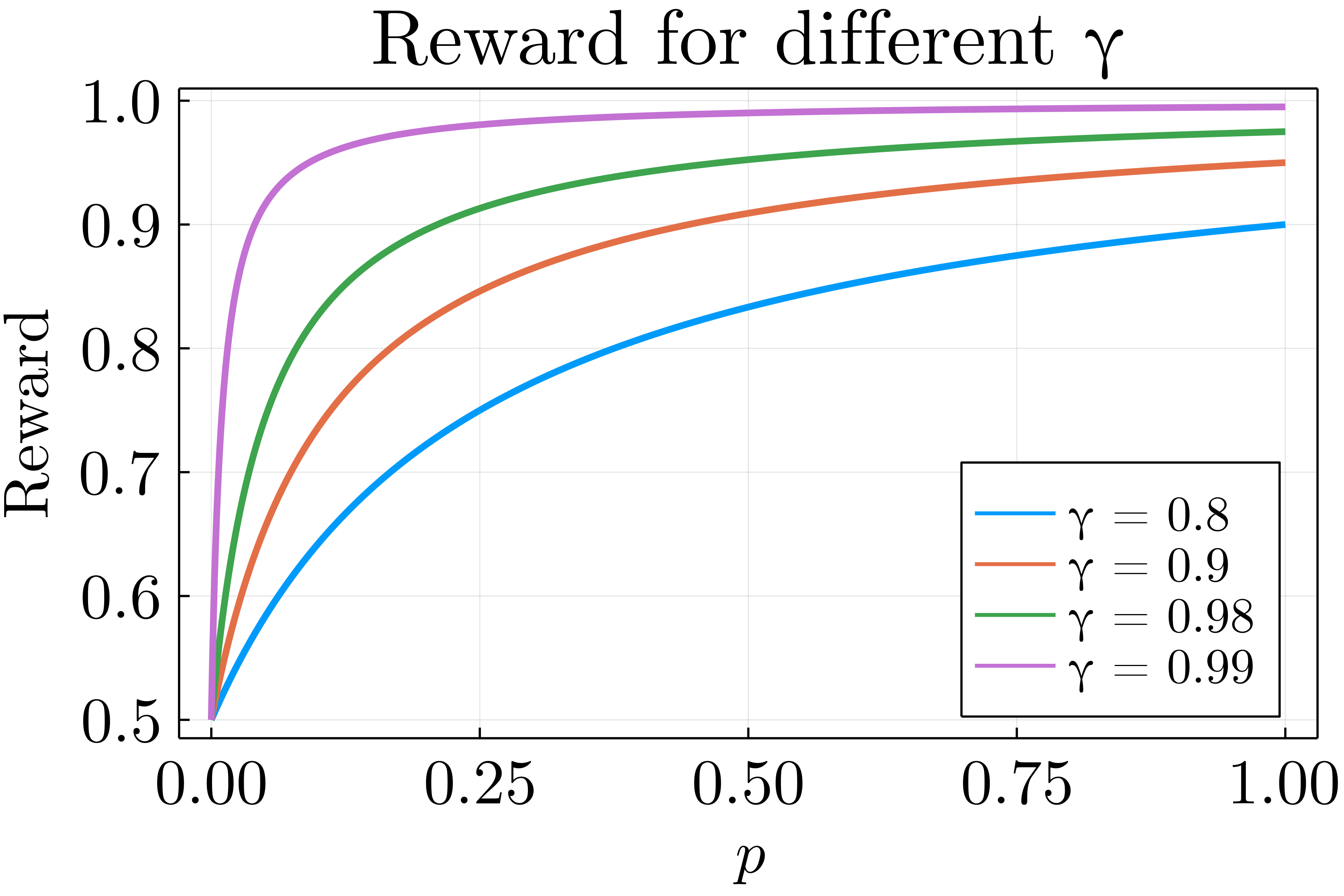
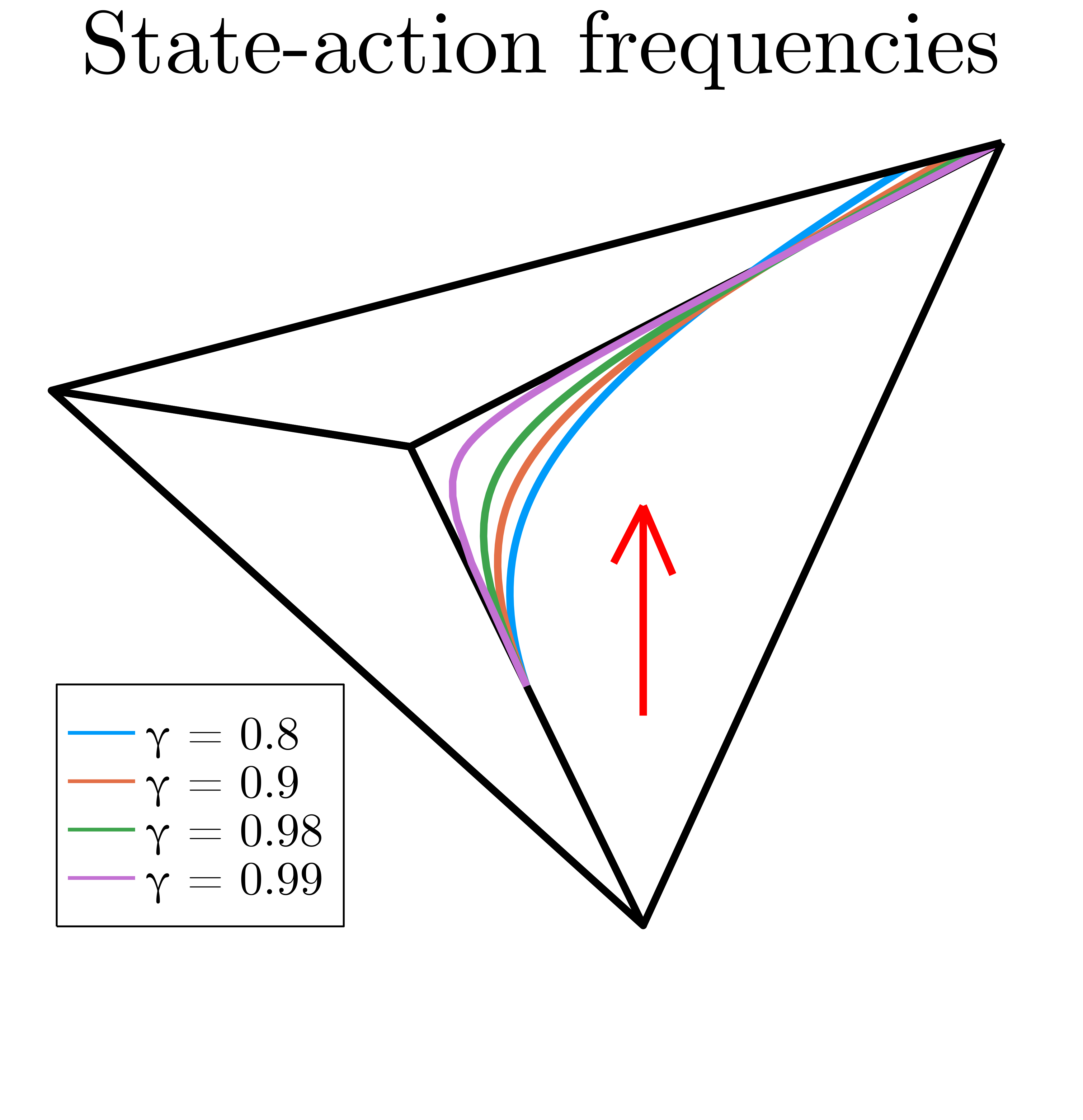
Figure 1: A blind controller with two states; policies can be parameterized by $p\in[0,1]$; for increasing $\gamma$ the Lipschitz constant of the reward increases (left); the corresponding feasible state-action frequencies, probability simplex $\Delta_{\SS\times\mathcal{A}}$, and instantaneous reward vector (right).

Policy gradients

A very popular approach in Reinforcement Learning are policy gradients methods. In fully observable problems, the iteration complexity of policy gradient methods behaves like $O((1-\gamma)^{-\kappa})$, where $\gamma\in(0,1)$ is the discount factor and $\kappa\in\mathbb{N}$ depends on the specific method [CCC⁺21]. This is reminiscent of the Lipschitz constant of the reward function (as a function of the policy), which behaves like $O((1-\gamma)^{-1})$ [PRB15]; see Figure 1. This leads to increasingly ill-conditioned problems as $\gamma\to 1$ and can cause undesired oscillations during optimization [Wag11]. However, choosing a discount factor close to $1$ is desirable as one often wishes to optimize the mean reward rather than a discounted reward. This is also required to prevent vanishing policy gradients in sparse reward MDPs, where, denoting $n_{\SS}$ the number of states, gradients can of order $O(2^{-n_{\SS}/2})$ if $\gamma\leq n_{\SS}/(n_{\SS}+1)$ [AKLM21]. In principle the ill-conditioning problem can be addressed by introducing an appropriate metric, as in natural policy gradients or trust region policy optimization, which can be costly, however.

Optimization in state-action space

An alternative to optimizing over the policy parameters is to optimize the reward over all feasible state-action frequencies of the POMDP. State-action frequencies are weighted averages of the time spent by the Markov process at different state-action pairs. The reward of a policy depends linearly on its state-action frequency and the optimization in state-action space maximizes the time spend in favorable states. The policy corresponding to a state-action frequency can be recovered by conditioning over states. In MDPs, the state-action frequencies form a polytope and hence the problem becomes a linear program [Der70, Kal94]. This yields a strongly polynomial algorithmic approach, i.e., does not degrade for $\gamma\to 1$ [PY15]. In the case of POMDPs, additional polynomial constraints describe the set of all feasible state-action frequencies of POMDPs, which were recently described by  [MM22]. This yields a polynomial program of POMDPs generalizing the linear programs of MDPs. In this work we investigate the practical viability of this approach to optimize the reward in POMDPs. We consider navigation tasks in random mazes of different sizes, for which we develop a tool to generate the constraints and solve the constrained optimization problem using interior point methods. Our experiments show that the proposed method can yield significant computational savings compared to several baselines, while also remaining numerically stable across values of $\gamma$ where other methods fail.

2 Notation and setup

We denote the simplex of probability distributions on a finite set $\mathcal{X}$ by $\Delta_{\mathcal{X}}$ and the set of Markov kernels from a finite set $\mathcal{X}$ to another finite set $\mathcal{Y}$ by $\Delta_{\mathcal{Y}}^{\mathcal{X}}$. A partially observable Markov decision process or shortly POMDP is a tuple $(\mathcal{S},\mathcal{O},\mathcal{A},\alpha,\beta,r)$. We assume that $\mathcal{S},\mathcal{O}$ and $\mathcal{A}$ are finite sets which we call the state, the observation and the action space respectively. We fix a Markov kernel $\alpha\in\Delta_{\mathcal{S}}^{\mathcal{S}\times\mathcal{A}}$ which we call the transition mechanism and a kernel $\beta\in\Delta_{\mathcal{O}}^{\mathcal{S}}$ which we call the observation mechanism. Further, we consider an instantaneous reward vector $r\in\mathbb{R}^{\mathcal{S}\times\mathcal{A}}$. As policies we consider elements $\pi\in\Delta_{\mathcal{A}}^{\mathcal{O}}$, which are referred to as memoryless stochastic policies. Every policy defines a transition kernel $P_{\pi}\in\Delta_{\mathcal{S}\times\mathcal{A}}^{\mathcal{S}\times\mathcal{A}}$ by $P_{\pi}(s^{\prime},a^{\prime}|s,a)\coloneqq\alpha(s^{\prime}|s,a)\sum_{o}\pi(a^{\prime}|o)\beta(o|s^{\prime})$. For any initial state distribution $\mu\in\Delta_{\mathcal{S}}$, a policy $\pi\in\Delta_{\mathcal{A}}^{\mathcal{O}}$ defines a Markov process on $\mathcal{S}\times\mathcal{A}$ with transition kernel $P_{\pi}$ which we denote by $\mathbb{P}^{\pi,\mu}$. For a discount rate $\gamma\in(0,1)$ we define the infinite horizon expected discounted reward

$$R(\pi) \coloneqq\mathbb{E}_{\mathbb{P}^{\pi,\mu}}\left[(1-\gamma)\sum_{t=0}^{\infty}\gamma^{t}r(s_{t},a_{t})\right].$$ (1)

We consider the reward maximization problem, i.e., the problem of maximizing $R(\pi)$ subject to $\pi\in\Delta_{\mathcal{A}}^{\mathcal{O}}$. The discount factor $\gamma$ is most commonly introduced for mathematical convenience. For large state spaces and sparse rewards or more generally for POMDPs where the optimal policy should not depend on an unknown initial state distribution, it may be more desirable to consider the expected reward per time step, which corresponds to the limit $\gamma\to 1$.

3 Feasible state-action frequencies

It is well known that $R(\pi)=\langle r,\eta^{\pi}\rangle_{\SS\times\mathcal{A}}$, where $\eta^{\pi}(s,a)=(1-\gamma)\sum_{t\geq 0}\gamma^{t}\mathbb{P}^{\pi,\mu}(s_{t}=s,a_{t}=a)$ is the state-action frequency of $\pi$. We denote the set of feasible state-action frequencies in the fully observable and in the partially observable case by $\mathcal{N}$ and $\mathcal{N}_{\beta}$, respectively. Hence, instead of solving the reward maximization problem over $\pi$, one can also solve the reward maximization problem in state-action space, which is given by

$$\operatorname{maximize}\;\langle r,\eta\rangle\quad\text{subject to }\eta\in\mathcal{N}_{\beta}\subseteq\Delta_{\SS\times\mathcal{A}}.$$ (2)

To do this in practice, one requires a suitable characterization of the set of feasible state-action frequencies $\mathcal{N}_{\beta}$. To describe this set via polynomial conditions, we introduce the effective policy poltyope $\Delta_{\mathcal{A}}^{\SS,\beta}\coloneqq\{\pi\circ\beta:\pi\in\Delta_{\mathcal{A}}^{\mathcal{O}}\}$, which is the set of state policies that can be realized by selecting the actions based on observations made according to $\beta$. Note that the set of effective policies $\Delta_{\mathcal{A}}^{\SS,\beta}$ is a polytope since it is the image of the polytope $\Delta_{\mathcal{A}}^{\mathcal{O}}$ under the linear map $\pi\mapsto\pi\circ\beta$.

The state-action frequencies of an MDP

As mentioned before, the state-action frequencies of an MDP form a polytope $\mathcal{N}=\left\{\eta\in\mathbb{R}_{\geq 0}:\ell_{s}(\eta)=0\text{ for }s\in\SS\right\}\subseteq\Delta_{\SS\times\mathcal{A}}$, where $\ell_{s}(\eta)=\langle\delta_{s}\otimes\mathds{1}_{\mathcal{A}}-\gamma\alpha(s|\cdot,\cdot),\eta\rangle_{\SS\times\mathcal{A}}-(1-\gamma)\mu_{s}$; see [Der70]. Hence for MDPs the reward maximization problem (2) becomes a linear program in state-action frequency space. This is known as the dual linear programming formulation of MDPs [Kal94].

The state-action frequencies of a POMDP

The effective policy corresponding to a state-action frequency can be computed by conditioning. In order for the conditioning to be well defined, we require the following assumption, which holds for instance if the initial distribution $\mu$ has full support.

Assumption 1.

For any state-action frequency $\eta\in\mathcal{N}$ and any state $s\in\SS$ it holds that $\sum_{a}\eta_{sa}>0$. In the mean reward case we further assume that for every policy $\pi\in\Delta_{\mathcal{A}}^{\mathcal{O}}$ there exists a unique stationary distribution of $P_{\pi}$. This is a standard assumption in MDP linear programming [Kal94] and necessary for the convergence of PG methods [MXSS20].

The correspondence of state-action frequencies $\eta\in\mathcal{N}$ and state policies $\tau\in\Delta_{\mathcal{A}}^{\SS}$ via conditioning provides a correspondence of polynomial inequalities in the two sets $\Delta_{\mathcal{A}}^{\SS}$ and $\mathcal{N}$. More precisely, setting $S\coloneqq\{s\in\mathcal{S}:b_{sa}\neq 0\text{ for some }a\in\mathcal{A}\}$ it holds that

$$\sum_{s,a}b_{sa}\tau_{sa}\geq 0\quad\text{if and only if}\quad\sum_{s\in S}\sum_{a}b_{sa}\eta_{sa}\prod_{s^{\prime}\in S\setminus\{s\}}\sum_{a^{\prime}}\eta_{s^{\prime}a^{\prime}}\geq 0.$$ (3)

Therefore, the set of feasible state-action frequencies $\mathcal{N}_{\beta}$ can be described by finitely many polynomial (in)equalities corresponding to the linear (in)equalities describing $\Delta_{\mathcal{A}}^{\SS,\beta}$ in $\Delta_{\mathcal{A}}^{\SS}$. In particular, this shows that solving the reward optimization problem in infinite-horizon POMDPs with memoryless stochastic policies is equivalent to a polynomially constrained optimization problem with linear objective, which generalizes the lienar program associated to MDPs. This formulation was obtained in [MM22] and was used to establish upper bounds on the number of critical points of the reward optimization problem. In this work, we focus the solution of POMDPs via this polynomial program.

4 Reward optimization in state-action frequency space (ROSA)

We formulate our approach for Reward Optimization in State-Action space (ROSA) in Algorithm 1.

Algorithm 1 Reward Optimization in State-Action space (ROSA)

1:$\alpha\in\Delta_{\SS}^{\SS\times\mathcal{A}}$, $\beta\in\Delta_{\mathcal{O}}^{\SS}$, $\gamma\in(0,1)$, $\mu\in\Delta_{\SS}$

2:for all $s\in\mathcal{S}$ do

3:     $\ell_{s}(\eta)\leftarrow\langle\delta_{s}\otimes\mathds{1}_{\mathcal{A}}-\gamma\alpha(s|\cdot,\cdot),\eta\rangle_{\SS\times\mathcal{A}}-(1-\gamma)\mu_{s}$ $\triangleright$ Define the linear equalities

4:end for

5:Compute the defining linear inequalities of $\Delta_{\mathcal{A}}^{\SS,\beta}$ $\triangleright$ In closed form or algorithmically

6:Compute the defining polynomial inequalities $p_{i}(\eta)\geq 0$ of $\mathcal{N}_{\beta}$ $\triangleright$ Can be done according to (3)

7:$\eta^{\ast}\leftarrow\arg\max\langle r,\eta\rangle$ sbj to $\eta\geq 0$, $\ell_{s}(\eta)=0$ , $p_{i}(\eta)\geq 0$ $\triangleright$ Solve the constrained maximization problem

8:$R^{\ast}\leftarrow\langle r,\eta^{\ast}\rangle$ $\triangleright$ Evaluate the optimal value

9:$\tau^{\ast}\leftarrow\eta^{\ast}(\cdot|\cdot)\in\Delta_{\mathcal{A}}^{\mathcal{S}}$ $\triangleright$ Compute an optimal state policy

10:$\pi^{\ast}\leftarrow$ solution of $\beta\pi=\tau^{\ast}$ $\triangleright$ Compute an optimal observation policy return $\eta^{\ast}$, $R^{\ast}$, $\pi^{\ast}$ $\triangleright$ maximizer, optimal value, optimal policy

The two non-trivial steps in the algorithm are the computation of the defining linear inequalities of the polytope $\Delta_{\mathcal{A}}^{\SS,\beta}$ in line 5 and the solution of the constrained optimization problem in line 7.

Computing the polynomial constraints

The linear inequalities defining $\Delta_{\mathcal{A}}^{\SS,\beta}$ and therefore the polynomial constraints of $\mathcal{N}_{\beta}$ can be computed in closed form if $\beta$ has linear independent columns [MM22, Thm. 12]. If this is not the case, they can be computed algorithmically using Fourier-Motzkin elimination, block elimination, vertex approaches, or equality set projection [JKM04]. Let us discuss the special case of deterministic observations. We associated $\beta$ with a mapping $\SS\to\mathcal{O}$, which partitions the state space into sets $S_{o}\coloneqq\{s\in\SS:\beta(o|s)=1\}\subseteq\mathcal{S}$. If we fix an arbitrary action $a_{0}\in\mathcal{A}$ and arbitrary states $s_{o}\in S_{o},o\in\mathcal{O}$, the polynomial equations cutting out the set $\mathcal{N}_{\beta}$ of feasible state-action frequencies from the set $\mathcal{N}$ of all state-action frequencies are given by

$$p^{o}_{sa}(\eta)\coloneqq\eta_{s_{o}a}\sum_{a^{\prime}}\eta_{sa^{\prime}}-\eta_{sa}\sum_{a^{\prime}}\eta_{s_{o}a^{\prime}}=\sum_{a^{\prime}\neq a}(\eta_{s_{o}a}\eta_{sa^{\prime}}-\eta_{s_{o}a^{\prime}}\eta_{sa})=0,$$ (4)

for all actions $a\in\mathcal{A}\setminus\{a_{0}\}$, states $s\in S_{o}\setminus\{s_{o}\}$ and observations $o\in\mathcal{O}$. Hence, for deterministic observations the reward maximization problem in state-action space takes the form

$$\operatorname{maximize}\;\langle r,\eta\rangle\quad\text{subject to }\left\{\begin{array}[]{rl}\ell_{s}(\eta)=0&\text{for }s\in\mathcal{S}\\ p_{sa}^{o}(\eta)=0&\text{for }o\in\mathcal{O},a\in\mathcal{A}\setminus\{\tilde{a}\},s\in S_{o}\setminus\{s_{o}\}\\ \eta_{sa}\geq 0&\text{for }s\in\SS,a\in\mathcal{A}.\end{array}\right.$$ (5)

This is a problem in $\lvert\SS\rvert\lvert\mathcal{A}\rvert$ variables with $\lvert\SS\rvert$ linear and $\sum_{o}(\lvert S_{o}\rvert-1)(\lvert\mathcal{A}\rvert-1)=(\lvert\SS\rvert-\lvert\mathcal{O}\rvert)(\lvert\mathcal{A}\rvert-1)$ quadratic equality constraints and $\lvert\SS\rvert\lvert\mathcal{A}\rvert$ inequality constraints (of which only $\lvert\mathcal{O}\rvert\lvert\mathcal{A}\rvert$ are non redundant).

Implementation and solution of the optimization problem

We provide a Julia [BEKS17] implementation of ROSA for deterministic observations. In general, problem (5) can be solved with any constrainted optimization solver. Our implementation is built on Ipopt, an interior point line search method [WB06]. We call Ipopt via the modeling language JuMP in which the constraints are easy to implement [DHL17]. The implementation is available under https://github.com/muellerjohannes/POMDPs-ROSA.

5 Experiments

To demonstrate the performance of ROSA we test it on navigation problems in mazes. For this, we generate connected mazes using a random depth first search [maz]. Then we randomly select a state as the goal state at which a reward of $\lvert\SS\rvert$ is picked up and from which the agent transitions to a uniform state. For all other states four actions move the agent right, left, up or down. The agent can only observe the 8 neighboring cells and starts at a uniform position.

We compare against two other optimization approaches. First, we consider tabular softmax policies and directly optimize the parameters for the exact discounted reward. Instead of a vanilla policy gradient ascent, we use L-BFGS, which is a first order method that estimates second order information. In comparison to a naive policy gradient, we observed L-BFGS to converge faster. We refer to this approach as direct policy optimization (DPO). As a second baseline we consider the reformulation of the reward maximization problem as a quadratically constrained linear program [ABZ06]

$$\operatorname{maximize}\;\langle\mu,v\rangle\quad\text{subject to }\pi\in\Delta_{\mathcal{A}}^{\mathcal{O}}\text{ and }v=\gamma p_{\pi}v+(1-\gamma)r_{\pi},$$ (6)

where $p_{\pi}(s^{\prime}|s)\coloneqq\sum_{o,a}\pi(a|o)\beta(o|s)\alpha(s^{\prime}|s,a)$ and $r_{\pi}(s)\coloneqq\sum_{a,o}r(s,a)\pi(a|o)\beta(o|s)$.

Note that here the constraint is on the value function. We use Ipopt to solve (6). We call this approach Bellman constrained programming (BCP).

Figure 2: Shown is the solution time and cumulative reward obtained by different methods solving navigation tasks depending on the number of states or the discount factor. Inset shows one of the mazes with $199$ states. ROSA reaches higher reward in less time, with stability improvements and time savings becoming more pronounced for larger $\gamma$.

In order to compare the running times of the three approaches, we generate square mazes of side length $2n-1$ and $2n^{2}-1$ states, for $n=2,\dots,10$. We solve the POMDPs for a discount factor of $\gamma=0.9999$ using ROSA, BCP and DPO for $10^{2}$ different mazes of each size and report the mean solution times and achieved rewards as well as their $16\%$ and $84\%$ quantiles in Figure 2. We observe that all three methods achieve comparable rewards. However, DPO becomes inefficient even for problems of moderate size and the running time of BCP grows significantly faster compared to ROSA.

To evaluate the performance of ROSA for $\gamma\to 1$ we solve $10^{2}$ mazes with side length $9$ and $49$ states for increasing discount factors. We report the average solution times and achieved reward in Figure 2. In the comparison of the rewards, examples where BCP did not converge are excluded. In these experiments we see that BCP becomes unstable, whereas the solution time of ROSA appears to be very robust and even decrease for $\gamma\to 1$. In fact, in the solution of (6) Ipopt fails to converge to local optimality for about $15\%$ of all problems with discount factor at least $0.9999$.

References

- [ABZ06] Christopher Amato, Daniel S Bernstein, and Shlomo Zilberstein, Solving POMDPs using quadratically constrained linear programs, Proceedings of the fifth international joint conference on Autonomous agents and multiagent systems, 2006, pp. 341–343.
- [AKLM21] Alekh Agarwal, Sham M Kakade, Jason D Lee, and Gaurav Mahajan, On the theory of policy gradient methods: Optimality, approximation, and distribution shift, Journal of Machine Learning Research 22 (2021), no. 98, 1–76.
- [AYA18] Kamyar Azizzadenesheli, Yisong Yue, and Animashree Anandkumar, Policy gradient in partially observable environments: Approximation and convergence, arXiv preprint arXiv:1810.07900, 2018.
- [BEKS17] Jeff Bezanson, Alan Edelman, Stefan Karpinski, and Viral B Shah, Julia: A fresh approach to numerical computing, SIAM review 59 (2017), no. 1, 65–98.
- [CCC+21] Shicong Cen, Chen Cheng, Yuxin Chen, Yuting Wei, and Yuejie Chi, Fast global convergence of natural policy gradient methods with entropy regularization, Operations Research (2021).
- [Der70] C. Derman, Finite state Markovian decision processes, Tech. report, Columbia University, 1970.
- [DHL17] Iain Dunning, Joey Huchette, and Miles Lubin, JuMP: A modeling language for mathematical optimization, SIAM review 59 (2017), no. 2, 295–320.
- [JKM04] Colin Jones, E. C. Kerrigan, and Jan Maciejowski, Equality set projection: A new algorithm for the projection of polytopes in halfspace representation, Tech. report, University of Cambridge, 2004.
- [Kal94] L.C.M. Kallenberg, Survey of linear programming for standard and nonstandard Markovian control problems. Part I: Theory, Zeitschrift für Operations Research 40 (1994), no. 1, 1–42.
- [maz] Maze generation, https://rosettacode.org/wiki/Maze_generation, Accessed: 2022-01-10.
- [MM22] Johannes Müller and Guido Montúfar, The Geometry of Memoryless Stochastic Policy Optimization in Infinite-Horizon POMDPs, International Conference on Learning Representations, 2022.
- [MXSS20] Jincheng Mei, Chenjun Xiao, Csaba Szepesvari, and Dale Schuurmans, On the global convergence rates of softmax policy gradient methods, International Conference on Machine Learning, PMLR, 2020, pp. 6820–6829.
- [PRB15] Matteo Pirotta, Marcello Restelli, and Luca Bascetta, Policy gradient in Lipschitz Markov decision processes, Machine Learning 100 (2015), no. 2, 255–283.
- [PY15] Ian Post and Yinyu Ye, The simplex method is strongly polynomial for deterministic Markov decision processes, Mathematics of Operations Research 40 (2015), no. 4, 859–868.
- [SMS+99] Richard S Sutton, David A McAllester, Satinder P Singh, Yishay Mansour, et al., Policy gradient methods for reinforcement learning with function approximation, NIPs, vol. 99, Citeseer, 1999, pp. 1057–1063.
- [Wag11] Paul Wagner, A reinterpretation of the policy oscillation phenomenon in approximate policy iteration, Advances in Neural Information Processing Systems 24 (2011), 2573–2581.
- [WB06] Andreas Wächter and Lorenz T Biegler, On the implementation of an interior-point filter line-search algorithm for large-scale nonlinear programming, Mathematical programming 106 (2006), no. 1, 25–57.