Vehicle mission guidance by symbolic optimal control

Abstract

Symbolic optimal control is a powerful method to synthesize algorithmically correct-by-design state-feedback controllers for nonlinear plants. Its solutions are (near-)optimal with respect to a given cost function. In this note, it is demonstrated how symbolic optimal control can be used to calculate controllers for an optimized routing guidance of vehicle systems in continuous state space. In fact, the capacitated vehicle routing problem and a variant of travelling salesman problem are investigated. The latter problem has a relevant application in case of loss of vehicles during mission. A goods delivery scenario and a reconnaissance mission, involving bicycle and aircraft dynamics respectively, are provided as examples.

I Introduction

Vehicle routing problems exist in numerous variations and often reflect relevant problems in applied logistics [1, 2]. The raw vehicle routing problem (VRP) consists of a weighted graph and asks for a set of routes for a fleet of vehicles for visiting all “customer” nodes optimally when starting and returning to the “depot” node. Techniques of combinatorial optimization provide solvers for it which return either exact or approximately optimal solutions. Mostly, vehicle routing problems are posed on ordinary directed or undirected graphs. Thus, they neglect any kind of dynamics behind the routes. Some exceptions consider Dubins vehicle dynamics and a fixed variant of the VRP, e.g. [3, 4, 5]. In our preceding work [6], we considered the classical travelling salesman problem for arbitrary nonlinear dynamics.

This note follows the approach in our previous work, i.e. assumes nonlinear vehicle dynamics in discrete time and continuous state space. In fact, the dynamics are given by

$$x(t+1)\in F(x(t),u(t))$$ (1)

with state signal $x$ in $\mathbb{R}^{n}$, input signal $u$ and a strict set-valued map $F$. Customer locations as well as the depot are assumed by non-empty sets in $\mathbb{R}^{n}$ and the cost for the mission is obtained by accumulating a non-negative cost term along the routes. In our example sections, we consider vehicle dynamics which are given in continuous time and are subject to additive disturbances bounded in $W\subseteq\mathbb{R}^{n}$. In fact, the dynamics is given by the differential inclusion

$$\dot{x}\in f(x,u)+W$$ (2)

where $f$ is an ordinary map. By sampling, (2) is transferred to (1) making our methods applicable to dynamics (2).

The focus of this work is on two variants of the VRP, namely the capacitated vehicle routing problem (CVRP) and a dynamic variant of the travelling salesman problem (TSP). The algorithms to present will provably solve previous problems with respect to the qualitative task, i.e. the control task of visiting a prescribed set of targets under some further constraints on the order of visit. (In this work, we refer to this special coverage specification as “mission”.) In addition, we provide novel heuristics within the algorithms to quantitatively reduce the cost for the mission in total.

As we demonstrate, our methods can be used for general vehicle mission guidance and task reassignments. As an example for the latter, we consider reconnaissance missions with uninhabited aerial vehicles (UAVs) where at some point during mission a UAV suffers a damage. In this case, the remaining UAVs must take over the tasks of the broken UAV. This kind of scenario is not new, e.g. is investigated in [7, 8, 9]. In these works, nonlinear vehicle dynamics are basically neglected and solutions based on infinite digraphs are presented. A drawback of our approach is that our methodology does not ensure collision avoidance if the mission involves more than one vehicle.

To summarize, our novel methods solve coverage problems under certain additional constraints that involve nonlinear dynamics, hard state or input constraints, uncertainties or measurement errors. These features come out-of-the-box with correct-by-design controllers which have been heuristically optimized to reduce mission costs. To this end, the framework of symbolic optimal control [10] and the related computational means [11] are used.

The remaining part of this note is organized as follows. After introducing notation (Section II) a review on symbolic optimal control is given (Section III-A) and some known results on coverage problems are stated (Section III-B). Sections IV and V contain the novel methods on the CVRP and the dynamic TSP, respectively. Each of the two previous sections contains a subsection with an experimental evaluation. Conclusions are given in Section VI.

II Notation

The symbols $\mathbb{R}$, $\mathbb{R}_{+}$, $\mathbb{Z}_{+}$, $\mathbb{N}$ stand for the set of real numbers, the subset of non-negative real numbers, the set of non-negative integers and the set of positive integers, respectively. The closed and half-open intervals in $\mathbb{R}$ are denoted by $\left[a,b\right]$, $\left[a,b\right[$, $\left]a,b\right]$ for $a,b\in\mathbb{R}$. For discrete intervals, we write $\left[a;b\right]$, $\left[a;b\right[$, $\left]a;b\right]$, e.g. $\left]a;b\right]=\left]a,b\right]\cap\mathbb{Z}$. If $A,B$ are sets the notation $f\colon A\rightrightarrows B$ means that $f$ is a set-valued map. $f$ is strict if $f(a)\neq\emptyset$ for all $a\in A$, where $\emptyset$ stands for the empty set. If $f\colon A\times B\to C$ is an ordinary map then $f(\cdot,b)$ stands for the map $A\to C$ mapping $a$ to $f(a,b)$. If $f$, $g$ are maps then $f\circ g$ stands for the composition of $f$ and $g$. $A^{B}$ denotes the set of all (ordinary) maps $B\to A$. E.g. $A^{\mathbb{Z}_{+}}$ stands for the set of all sequences $(a_{0},a_{1},\ldots)$ with $a_{i}\in A$ for all $i\in\mathbb{Z}_{+}$. Elements of $A^{\mathbb{Z}_{+}}$ are called signals. The notation $(a_{i})_{i=1}^{k}$ stands for the finite sequence $(a_{1},\ldots,a_{k})$. The length of a finite sequence $a$ is denoted by $\operatorname*{len}a$, e.g. $\operatorname*{len}(a_{1},a_{2},a_{3})=3$.

III Review: Symbolic optimal control and quantitative coverage problems

We review the concept of symbolic optimal control as established in [10, 12] since the novel methods are built on top. Our methods also use basic techniques for solving quantitative reachability problems or more generally coverage problems. Therefore, a review on these specifications is also included.

III-A Symbolic optimal control

Our methods apply to dynamical systems that can be cast to transition systems. By the latter we mean a triple

$$(X,U,F)$$ (3)

which defines dynamics (1), where $F\colon X\times U\rightrightarrows X$ is a strict set-valued map. The non-empty sets $X$ and $U$ are called state and input space, respectively. Let $S$ denote (3). A controller for $S$ is a strict set-valued map

$$\mu\colon\bigcup_{T\in\mathbb{Z}_{+}}\nolimits X^{\left[0;T\right]}\rightrightarrows U\times\{0,1\}$$ (4)

and shall influence by concept the behaviour of $S$. The second component of the image of $\mu$ reports if the controller is indeed enabled (’$0$’) or disabled (’$1$’) [13]. In this work, controller (4) will be composed of several memoryless controllers $X\rightrightarrows U\times\{0,1\}$ as shown in Fig. 1.

Figure 1: Controller structure [6] used in this work. The scheduler switches between memoryless controllers $\mu_{1},\ldots,\mu_{K}\colon X\rightrightarrows U\times\{0,1\}$. Switching is triggered when the stopping signal $v$ of the active controller (gray) changes from $0$ to $1$.

The closed-loop behaviour (initialized at $p\in X$) is the set of all signals $(u,v,x)\in(U\times\{0,1\}\times X)^{\mathbb{Z}_{+}}$ that satisfy (1) and $(u(t),v(t))\in\mu(x|_{\left[0;t\right]})$ for all $t\in\mathbb{Z}_{+}$. This set is denoted by $\mathcal{B}_{p}(\mu\times S)$. In this work, the operation of the closed loop causes costs and the accomplishment of a control task in finite time is mandatory. In fact, the cost for operating the closed loop is given by virtue of the cost functional

$$J\colon(U\times\{0,1\}\times X)^{\mathbb{Z}_{+}}\to\mathbb{R}_{+}\cup\{\infty\}.$$ (5a)

It is defined by $$J(u,v,x)=\infty v$$ for perpetual operation, i.e. if the stopping signal is identically zero, and otherwise by

$$J(u,v,x)=G(x|_{\left[0;T\right]})+\sum_{t=0}^{T-1}g(x(t),x(t+1),u(t))$$ (5b)

where $T=\inf v^{-1}(1)<\infty$. In (5b), the trajectory cost

$$G\colon\bigcup_{T\in\mathbb{Z}_{+}}\nolimits X^{\left[0;T\right]}\to\mathbb{R}_{+}\cup\{\infty\}$$ (6)

rates the trajectory until stopping, while the running cost

$$g\colon X\times X\times U\to\mathbb{R}_{+}\cup\{\infty\}$$ (7)

is accumulative and takes also into account the input signal. All in all, an optimal control problem is as follows[12, 10].

III.1 Definition.

Let $(X,U,F)$ be a system and let $G$ and $g$ be as in (6) and (7). An optimal control problem is a 5-tuple

$$(X,U,F,G,g).$$ (8)

The goal of symbolic optimal control is to find a controller so that the operation of the closed loop is at finite cost and ideally minimized for the worst case trajectory. To formalize this goal, we review the notion of closed-loop performance and value function. Subsequently, $\mathcal{F}(X,U)$ denotes the set of all controllers of the form (4).

III.2 Definition.

Let $\Pi$ be the optimal control problem in (8). Let $J$ be the cost functional (5) as defined for $\Pi$. The map $L\colon X\times\mathcal{F}(X,U)\to\mathbb{R}_{+}\cup\{\infty\}$ defined by

$$L(p,\mu):=\sup_{(u,v,x)\in\mathcal{B}_{p}(\mu\times S)}J(u,v,x)$$

is called performance function of $\Pi$. The closed-loop performance of $\mu\in\mathcal{F}(X,U)$ is the function $L(\cdot,\mu)$.

As usually in optimal control, the value function is related to the best possible closed-loop performance. Our methods will actually return suboptimal solutions, which are also defined next and turn out to be useful in applications.

III.3 Definition.

Let $\Pi$ and $L$ be as in Definition III.2. The value function of $\Pi$ is the map assigning $p\in X$ to

$$V(p):=\inf_{\nu\in\mathcal{F}(X,U)}L(p,\nu).$$ (9)

Let $A\subseteq X$ and let $\mu\in\mathcal{F}(X,U)$. The controller $\mu$ solves $\Pi$ suboptimally on $A$ if $V(p)<\infty$ implies $L(p,\mu)<\infty$ for all $p\in A$. $\mu$ is optimal if $V=L(\cdot,\mu)$ and the pair $(V,\mu)$ is an optimal solution of $\Pi$.

III-B Quantitative reach-avoid and coverage problems

In the special case that $\Pi$ in Def. III.3 is a quantitative reach-avoid problem and $X$ and $U$ are finite, computational techniques are available to solve $\Pi$. These techniques are the algorithmic core of the novel methods to present and briefly described subsequently.

A quantitative reach-avoid problem asks to steer the state of the system to a specified target set in finite time while minimizing the cost functional $J$ in (5). The constraint of obstacle avoidance can be formulated using the running cost (7) [10, Ex. III.5]. The precise definition is:

III.4 Definition (​​[12]).

Let $\Pi$ be an optimal control problem of the form (8) such that $G$ is defined by

$$G(x|_{\left[0;t\right]})=\begin{cases}G_{0}(x(t)),&\text{if }x(t)\in A\\ \infty,&\text{otherwise}\end{cases}$$

where $A\subseteq X$ non-empty and $G_{0}\colon X\to\mathbb{R}_{+}\cup\{\infty\}$. Then $\Pi$ is called (quantitative) reach-avoid problem associated with $S$, $g$, $A$ and $G_{0}$, where $S$ denotes the system $(X,U,F)$.

The parameter function $G_{0}$ above is significant [12] in order to achieve partial optimality for the type of coverage problems considered in this work. The next definition generalizes Def. III.4. In fact, coverage asks to steer the system state to a given list of target sets in finite time (in any order).

III.5 Definition.

Let $S$ and $\Pi$ be as in Def. III.4 such that $G$ is defined by

$$G(x|_{\left[0;t\right]})=\begin{cases}G_{0}(x|_{\left[0;t\right]}),&\text{if }\ \forall_{i\in\left[1;N\right]}\exists_{s\in\left[0;t\right]}:x(s)\in A_{i}\\ \infty,&\text{otherwise}\end{cases}$$

where $A_{1},\ldots,A_{N}\subseteq X$ are non-empty and $G_{0}\colon\cup_{T\in\mathbb{Z}_{+}}X^{\left[0;T\right]}\to\mathbb{R}_{+}\cup\{\infty\}$. Then $\Pi$ is called (quantitative) coverage problem associated with $S$, $g$, $A_{1},\ldots,A_{N}$ and $G_{0}$.

By means of $G_{0}$ further constraints to a coverage problem on the trajectory can be added. A coverage problem associated with $G_{0}$ defined as identically $0$ can be solved by the fixed-point iteration algorithm shown in Fig. 2.

1:function SolveCoverage($S,g,A_{1},\ldots,A_{N}$)

2:     $Q\leftarrow\{1,\ldots,N\}$$\triangleright$ Initialize a queue

3:     $(A_{1}^{\prime},\ldots,A_{N}^{\prime})\leftarrow(A_{1},\ldots,A_{N})$$\triangleright$ Subsets of targets

4:     while $Q\neq\emptyset$ do

5:         Pick $i\in Q$

6:         $Q\leftarrow Q\setminus\{i\}$

7:         $(V_{i},\mu_{i})\leftarrow\textsc{SolveReach}(S,g,A_{i}^{\prime},0)$

8:         for all $j\in\{1,\ldots,N\}\setminus\{i\}$ do

9:              $A_{\mathrm{tmp}}\leftarrow A^{\prime}_{j}\setminus V_{i}^{-1}(\infty)$$\triangleright$ $A_{\mathrm{tmp}}\subseteq A^{\prime}_{j}$

10:              if $A_{\mathrm{tmp}}=\emptyset$ then$\triangleright$ Solving failed

11:                  return “Problem can’t be solved”

12:              else if $A^{\prime}_{j}\neq A_{\mathrm{tmp}}$ then

13:                  $A^{\prime}_{j}\leftarrow A_{\mathrm{tmp}}$$\triangleright$ Shrink $A^{\prime}_{j}$

14:                  $Q\leftarrow Q\cup\{j\}$$\triangleright$ Solve again for $j$

15:              end if

16:         end for

17:     end while

18:     return $((V_{1},A_{1}^{\prime},\mu_{1}),\ldots,(V_{N},A_{N}^{\prime},\mu_{N}))$

19:end function

Figure 2: Algorithm to solve the coverage problem associated with $S$, $g$, $A_{1},\ldots,A_{N}$ and the zero function [6].

It returns on success a sequence of triples $(V_{i},A_{i}^{\prime},\mu_{i})_{i=1}^{N}$, where $(V_{i},\mu_{i})$ is an optimal solution of the quantitative reach-avoid problem associated with $S$, $g$, $A_{i}^{\prime}$ and the zero function. Moreover, $V_{i}(p)<\infty$ for all $p\in\cup_{i=1}^{N}A_{j}^{\prime}$. See [6, Th. V.1] for a proof for correctness of the algorithm in Fig. 2. Key ingredient of this algorithm is the procedure

$$\textsc{SolveReach}(S,g,A,H),$$ (10)

which returns a pair of value function and optimal controller for the reach-avoid problem associated with $S$, $g$, $A$ and $H$.

Computational techniques realizing this procedure in case of discrete data can be found in [10, 14, 15, 16]. In combination with symbolic controller synthesis [11] procedure (10) can be realized for sampled-data systems, whose underlying dynamics take the form (2). Fig. 3 depicts the principle.

Figure 3: Principle of symbolic controller synthesis [11, 12].

The given optimal control problem $\Pi$, which involves the sampled-data system $(X,U,F)$, is abstracted to an auxiliary optimal control problem $\Pi^{\prime}$ that possesses finite state and input space $X^{\prime}$ and $U^{\prime}$, respectively. $X^{\prime}$ is a finite cover of $X$ by non-empty sets and $U^{\prime}$ a finite subset of $U$. $\Pi^{\prime}$ is solved algorithmically. The resulting controller $\mu^{\prime}$ is interconnected with a quantizer $Q\colon X\rightrightarrows X^{\prime}$ and the composition $\mu^{\prime}\circ Q$ solves $\Pi$ suboptimally on a predefined subset of $X$ [10]. Convergence results exist [10]. $Q$ is defined by $\Omega\in Q(x)$ iff $x\in\Omega$. Applying this principle to coverage problems by means of Fig. 2 results (on success) in controllers $\mu_{1},\ldots,\mu_{N}$. The controller $\mu_{i}$ steers the state signal near-optimally to $A_{i}$ whenever the state signal starts in $\cup_{i=1}^{N}A_{i}^{\prime}$.

This principle will be applied in our simulation results.

IV Capacitated vehicle routing problem

In this section, our contributions on the CVRP are presented beginning with the problem definition, the proposed heuristic optimization, and concluding with simulation results. Our contributions generalize those in [6, Sect. V].

IV-A Problem definition and heuristic optimization

Firstly, we review the classical definition of a CVRP and then we transfer it to our continuous domain.

In a classical capacitated VRP, a depot is given, $N-1$ customer locations, distances between all customers and the depot, and a vehicle capacity $q$. A set of tours is sought such that 1) all customers are served from the depot, 2) a vehicle visits at most as many customers as its capacity, and 3) a given objective function is minimized along the tours.

E.g., given three customers $2,3,4$ and depot $1$ with distance $1$ between each of them and vehicle capacity $2$ then the tours $1\to 2\to 1$ and $1\to 3\to 4\to 1$ constitute an optimal solution minimizing the total distance travelled, which is $5$.

In what follows, we formalize the notions of tour, CVRP and its solutions in the variant that is considered in this work.

IV.1 Definition.

Let $N\in\mathbb{Z}$, $N\geq 3$. A finite sequence

$$(1,t_{2},\ldots,t_{N-1},1)$$

where $t_{i}\in\mathbb{N}$, $t_{i}\geq 2$ for all $i\in\left[2;N\right[$ and $t_{i}\neq t_{j}$ for all $i\neq j$ is called $q$-tour for each $q\geq N-2$.

Therefore, a vehicle of capacity $q$ can perform at most a $q$-tour. The rigorous definition of the problem on a digraph with $N$ nodes and weighted adjacency matrix $C$ is as follows.

IV.2 Definition.

The triple

$$(N,q,C)\in\mathbb{N}\times(\mathbb{N}\cup\{\infty\})\times\mathbb{R}^{N\times N}$$ (11)

is called a classical (capacitated) vehicle routing problem with vehicles of (uniform) capacity $q$ and $N$ targets. A feasible sequence of $q$-tours to (11) is sequence of $q$-tours

$$(\mathcal{T}_{1},\ldots,\mathcal{T}_{m})$$ (12)

such that $\mathcal{T}_{1},\ldots,\mathcal{T}_{m}\in\cup_{T=3}^{N+1}\left[1;N\right]^{\left[1;T\right]}$ and all elements of $\left]1;N\right]$ appear exactly once in (12). An optimal solution of (11) is a feasible sequence of $q$-tours (12) that minimizes

$$\sum_{k=1}^{m}\nolimits\sum_{i=2}^{\operatorname{len}\mathcal{T}_{k}}\nolimits C_{\mathcal{T}_{k}(i-1),\mathcal{T}_{k}(i)}.$$ (13)

In the definition above, non-uniform customer demands are not considered and the number of tours/vehicles $m$ is part of the solution and not a constraint. However, the algorithm we are about to present immediately can be adopted to other problem variants including, e.g., individual customer demands or the multiple travelling salesman problem [17]. Also, other objectives than (13) can be considered.

Definition IV.2 is transferred to the continuous domain as follows. Although it is cumbersome to read, the idea is obvious. The constraint on the limited number of costumer supplies between two visits of the depot is modelled by means of $G_{0}$ in Def. III.5 and using (12).

IV.3 Definition.

Let $q\in\mathbb{N}$. Let $\Pi$ be a coverage problem associated with $S$, $g$, $A_{1},\ldots,A_{N}$ and $G_{0}$ defined by: $G_{0}(x|_{\left[0;t\right]})=0$ if there exist a feasible sequence of $q$-tours $(\mathcal{T}_{1},\ldots,\mathcal{T}_{m})$ such that for every $k,k^{\prime}\in\left[1;m\right]$, $k\leq k^{\prime}$ there exist $t_{1}\leq\ldots\leq t_{\operatorname*{len}\mathcal{T}_{k}}\leq t_{2}^{\prime}\leq\ldots\leq t^{\prime}_{\operatorname*{len}\mathcal{T}_{k^{\prime}}}$ such that

$$\forall_{l\in\left[1;\operatorname*{len}\mathcal{T}_{k}\right]}:x(t_{l})\in A_{\mathcal{T}_{k}(l)}\wedge\forall_{l\in\left]1;\operatorname*{len}\mathcal{T}_{k^{\prime}}\right]}:x(t^{\prime}_{l})\in A_{\mathcal{T}_{k^{\prime}}(l)}.$$

Otherwise, $G_{0}(x|_{\left[0;t\right]})=\infty$. Then $\Pi$ is called capacitated vehicle routing problem associated with $S$, $g$, target sets $A_{1},\ldots,A_{N}$ and capacity $q$. The set $A_{1}$ is called depot.

Using the algorithmic methods of symbolic optimal control as depicted in Section III, we can deduce a powerful heuristic to solve $\Pi$ in Def. IV.3 suboptimally. Algorithm 1 below provides controllers for each involved $q$-tour, which are heuristically optimized to reduce the cost functional (5) as defined for $\Pi$.

Algorithm 1 Capacitated vehicle routing problem

1:$S$, $g$, $A_{1},\ldots,A_{N}$, capacity $q$

2:$(\bar{V}_{i},A_{i}^{\prime},\bar{\mu}_{i})_{i=1}^{N}\leftarrow\textsc{SolveCoverage}(S,g,A_{1},\ldots,A_{N})$

3:if line 2 failed then

4:     return “Problem can’t be solved”

5:end if

6:Define $C\in\mathbb{R}^{N\times N}$ s. that $C_{i,j}=\min\{\bar{V}_{j}(p)\mid p\in A_{i}^{\prime}\}$

7:$(\mathcal{T}_{1},\ldots,\mathcal{T}_{m})\leftarrow$ solution of classical VRP $(N,q,C)$

8:for all $k\in\left[1;m\right]$ do

9:     for all $i\in\left[1;\operatorname*{len}\mathcal{T}_{k}\right[$ do

10:         $(V_{i},\mu_{k,i})\leftarrow\textsc{SolveReach}(S,g,A_{\mathcal{T}_{k}(i)},\bar{V}_{\mathcal{T}_{k}(i+1)})$

11:     end for

12:end for

13:$\mu_{1,1},\ldots,\mu_{m,\operatorname{len}\mathcal{T}_{m}}$

The algorithm works as follows.
1st part (lines 2–5). The coverage problem is solved. If successful (line 3) the following steps will heuristically optimize the cost by computing suitable $q$-tours.
2nd part (lines 6–7). A classical CVRP is solved (line 7), where the value functions obtained before serve as cost estimates between the sets $A_{1},\ldots,A_{N}$ (line 6). The involved minimum is a heuristic choice and is relevant in the 3rd part.
3rd part (lines 8–12). Finally the actual controller is computed. This last part builds upon the theoretical results in [12, Sect. III] and is of significant importance to optimize the trajectory of each tour. In fact, in line 10 an optimal controller is computed for reaching firstly $A_{\mathcal{T}_{k}(i)}$ and then $A_{\mathcal{T}_{k}(i+1)}$. Therefore, the minimum value in line 6 is a good estimate for the cost occurring between two targets.
Output (and correctness). The controller for the $q$-tour $\mathcal{T}_{k}$, $k\in\left[1;m\right]$ consists of the memoryless controllers $\mu_{k,1},\ldots,\mu_{k,\operatorname*{len}\mathcal{T}_{k}}$ and is assembled as in Fig. 4. Specifically, the controller $\mu_{k,j}$ steers a state signal starting in $\cup_{i=1}^{N}A^{\prime}_{i}$ to $A_{\mathcal{T}_{k}(j)}$. This key property of Algorithm 1 is due to line 2 since line 10 does not change the suboptimality of $\mu_{k,j}$ [6].

IV-B Experimental evaluation

As an example for the application of Algorithm 1, we consider a delivery truck in an urban environment as shown in Fig. 4. (This scenario extends the one in [6].) The truck has capacity $3$ and shall visit the $8$ target areas $A_{2},\ldots,A_{9}$ that are coloured in red. The depot ($A_{1}$) is coloured in green.

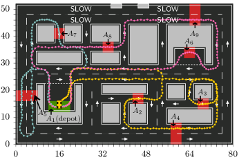
Figure 4: Truck delivery scenario of Section IV-B.

IV-B1 Truck dynamics

The truck is modelled in four dimensions according (2) with $(x_{1},x_{2})$ being its position in the plane, and $x_{3}$ and $x_{4}$ its orientation and velocity, respectively. Control inputs are the acceleration $u_{1}$ and the steering angle $u_{2}$. In fact, (2) is defined through $f\colon\mathbb{R}^{4}\times U\to\mathbb{R}^{4}$,

$$f(x,u)=$$

$$(x_{4}\cos(\alpha+x_{3})\cdot\beta,x_{4}\sin(\alpha+x_{3})\cdot\beta,x_{4}\tan(u_{2}),u_{1}),$$

where $U=\left[-6,4\right]\times\left[-0.5,0.5\right]$, $\alpha=\arctan(\tan(u_{2})/2)$, $\beta=\cos(\alpha)^{-1}$, $W=\{(0,0)\}\times\left[-0.01,0.01\right]\times\left[-0.1,0.1\right]$. This control system is sampled with period $\tau=0.1$ and a transition system $S$ in (3) is obtained with $X=\mathbb{R}^{4}$ and $U$ as above [11, Def. VIII.1].

IV-B2 Mission

Formally, the capacitated vehicle routing problem $\Pi$ associated with $S$, $g$, target sets $A_{1},\ldots,A_{9}$ and capacity $3$ is solved, where the involved objects are as follows. The coordinates of the target sets can be taken from Fig. 4 and are similar to, e.g., $A_{6}=\left[62,66\right]\times\left[32,36\right]\times\mathbb{R}\times\left[0,7\right].$ The running cost $g$ satisfies $g(x,y,u)=\infty$ in three cases; 1) if $x$ is outside the mission area

$$\left[0,80\right]\times\left[0,52\right]\times\mathbb{R}\times\left[0,18\right],$$ (14)

2) if $x$ is in one of the spacial obstacles depicted in Fig. 4 (gray coloured) or 3) if $x$ violates the common right-hand traffic rules. E.g. the scenario contains a speed limit in the northernmost east-west road, so $x$ being in the set

$$\left[0,80\right]\times\left[48,52\right]\times I_{\mathrm{east}}\times\left[0,12.5\right],I_{\mathrm{east}}=\left[-\tfrac{3\pi}{8},\tfrac{3\pi}{8}\right]$$

makes $g$ finite. If $g$ is finite, then $g$ balances minimum time and proper driving style. In fact,

$$g(x,y,u)=\tau+u_{2}^{2}+\min_{m\in M}\|(y_{1},y_{2})-m\|_{2},$$ (15)

where $M\subseteq\left[0,30\right]\times\left[0,50\right]$. $M$ describes the axes of the roadways, e.g. $\left[2,50\right]\times\{2\}\subseteq M$, and proper approaches to the depot (see [6, Sect. VI.B]) and to target set $A_{6}$, e.g.

$$\big{(}\{60\}\times\left[28,34\right]\big{)}\cup\big{(}\{68\}\times\left[28,34\right]\big{)}\cup\big{(}\left[60,68\right]\times\{34\}\big{)}\subseteq M.$$

IV-B3 Application of Algorithm 1

Algorithm 1 is applied to an abstracted problem $\Pi^{\prime}$ of $\Pi$ (cf. Fig. 3), where lines 2 and 10 are performed using value iteration [15] and line 7 by [18]. The problem $\Pi^{\prime}$ contains a discrete abstraction $(X^{\prime},U^{\prime},F^{\prime})$ with $|X^{\prime}|=150\cdot 114\cdot 62\cdot 50\approx 53\cdot 10^{6}$, $|U^{\prime}|=9\cdot 11$. Here, the factors indicate how the abstraction is constructed on (14) and $U$ [11]. While the algorithm runs, $20$ reach-avoid problems are solved in $51$ minutes average. Total runtime is $17$ hours using $41$ GB RAM in parallel computation with $26$ threads on Intel Xeon E5-2697 @ $2.60$ GHz.

IV-B4 Obtained solution and evaluation

The algorithm returns the three tours $\mathcal{T}_{1}=(1,3,4,2,1)$, $\mathcal{T}_{2}=(1,5,7,1)$, $\mathcal{T}_{3}=(1,8,9,6,1)$. The cost (5) for the mission beginning at the initial state $(16,14,\pi/2,0)$ is $244.6$. Fig. 4 shows the trajectory of this mission. To rate the capabilities of our heuristic, we consider the tours $(1,2,4,1)$, $(1,5,7,8,1)$, $(1,9,3,6,1)$, which are a “reasonable” manual choice. Those tours have total cost $248.5$, which is $1.6\%$ more than the solution returned by Algorithm 1. We would like to emphasize that in this example Algorithm 1 not only returns a proper choice but also relieves the engineer of the task of picking tours among $8!=40320$ possible choices.

V Travelling salesman problem
with arbitrary initial state

In this section, a technique for solving a travelling salesman problem is presented where the initial state of the salesman is not necessarily inside the depot but can be somewhere in the state space.

V-A Motivating example

We would like to give a concrete example to which the algorithm to be presented can be applied. We consider a reconnaissance mission [6], where two UAVs have to visit 40 areas of interest at minimum cost. The UAVs start and must return to the airfield, avoid obstacles, and share the task of visiting the areas. See Fig. 5(a). As stated, this is a VPR with a fixed number of vehicles of infinite capacity. A controller for the mission can be obtained by Algorithm 1 (by adding the constraint of a fixed number of vehicles to line 7). Now, we assume that at some random point in time during mission one UAV suffers damage and must return to base right away. The remaining UAV shall fly to all not yet visited areas of interest including those initially assigned to the other UAV. See Fig. 5(b). In this case, a TSP must be solved with initial state the current state of the functioning UAV. And clearly, the problem must be solved in short time so that the UAV can continue its mission without notable delay.

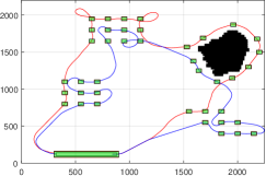
(a)

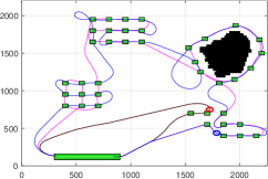
(b)

Trajectory	Cost
Red Fig. 5(a)	193
Blue Fig. 5(a)	222
Blue Fig. 5(b)	420
Magenta Fig. 5(b)	382

Lines Alg. 2	Runtime
3	60 min.
4 – 15	$<$ 2 sec.
16 – 23	8 min.
17 with $\rho=360$	10-15 sec.

(c)

Figure 5: Reconnaissance mission with 2 UAVs in Section V. The UAVs shall together visit all of the 40 areas of interest (small green-coloured rectangles). The UAVs start from the airfield (green box near the bottom) and must return to it. (a) Trajectories of the two UAVs (coloured blue and red, respectively) in a mission without UAV failure. (b) Mission where the UAV coloured in red suffers damage at the red-circled state. The UAV on the blue-coloured trajectory takes over the whole mission at the blue-circled state according to the result of Algorithm 2 (blue-coloured) and a comparison heuristic (magenta-coloured). (c) Computational details to the missions depicted in (a) and (b). Implementation uses $24$ threads on Intel Xeon E5-2697 @ $2.60$ GHz.

V-B Problem definition and heuristic optimization

Formally, we consider the following problem.

V.1 Definition.

Let $\Pi$ be a coverage problem associated with $A_{1},\ldots,A_{N}\subseteq X$ and $G_{0}$ defined by $G_{0}(x_{\left[0;t\right]})=\infty$ if $x(t)\notin A_{1}$ and otherwise $G_{0}(x_{\left[0;t\right]})=0$. Then $\Pi$ is called travelling salesman problem with target sets $A_{1},\ldots,A_{N}$. The set $A_{1}$ is called depot.

The algorithm below provides a suboptimal solution of the travelling salesman problem that is heuristically optimized for trajectories starting at the fixed initial state $x_{0}$. Moreover, it includes a technique to speed up computing time. The structure is similar to the one of Algorithm 1:

Algorithm 2 TSP with arbitrary initial state

1:$S=(X,U,F)$, $g$, $A_{1},\ldots,A_{N}$, initial state $x_{0}\in X$

2:$\rho\in\mathbb{R}_{+}$

3:$(V_{i},A_{i}^{\prime},\mu_{i})_{i=1}^{N}\leftarrow\textsc{SolveCoverage}(S,g,A_{1},\ldots,A_{N})$

4:if line 2 failed or $V_{1}(x_{0})=\infty$ then

5:     return “Problem can’t be solved”

6:end if

7:for all $i,j\in\{1,\ldots,N\}$ do

8:     if $i=1\text{ and }j>1$ then

9:         $C_{1,j}\leftarrow V_{j}(x_{0})$

10:     else

11:         $C_{i,j}\leftarrow\min\{V_{j}(p)\mid p\in A_{i}^{\prime}\}$

12:     end if

13:end for

14:$\mathcal{T}\leftarrow$ solution of classical VRP $(N,\infty,C)|_{\text{no. of vehicles}=1}$

15:Define $h_{i}\colon X\times X\times U\to\mathbb{R}_{+}\cup\{\infty\}$, $i\in\left[1;N\right]$ by:

$$h_{i}(x,y,u)=\begin{cases}g(x,y,u),&\text{if }\forall_{j\in\left[1;n\right]}\inf_{a\in A_{i}}\limits|x_{j}-a_{j}|\leq\rho\\ \infty,&\text{otherwise}\end{cases}$$

16:for all $i\in\left[1;N\right[$ do

17:     $(\bar{V}_{i},\bar{\mu}_{i})\leftarrow\textsc{SolveReach}(S,h_{i},A_{\mathcal{T}(i)},V_{\mathcal{T}(i+1)})$

18:     for all $x\in X$ do

19:         if $\bar{V}_{i}(x)=\infty$ then

20:              $\bar{\mu}_{i}(x)=\mu_{i}(x)$

21:         end if

22:     end for

23:end for

24:$\bar{\mu}_{1},\ldots,\bar{\mu}_{N}$

1st part (lines 3–6). The coverage problem is solved (line 3). If successful (including $x_{0}$), the algorithm continues.
2nd part (lines 7–14). A classical travelling salesman problem is solved, where the underlying weighted adjacency matrix $C$ is roughly defined as follows. In the first row the estimated costs for the initial state $x_{0}$ to the targets $A_{2},\dots,A_{N}$ appear (lines 7–13), where the previously computed value functions serve as cost estimates. Otherwise, the best-possible cost from $A_{i}$ to $A_{j}$ is contained in $C_{i,j}$ [12].
3rd part (lines 15–23). The actual controllers are computed. As seen in Section IV-B, this is time consuming if all the occurring reach-avoid problems (line 17) are fully solved. Therefore, in Algorithm 2 the reach-avoid problems are only solved on the neighbourhood of $A_{i}$, which is quantified by the parameter $\rho$. Finally, the controllers are combined with the already computed controllers of the coverage specification. In this way, line 17 can be executed while the closed loop is active at the sacrifice of further optimality.
Output (and correctness). Controller $\bar{\mu}_{i}$ steers a state signal stating in $\{x_{0}\}\cup A_{1}\cup\ldots\cup A_{N}$ to $A_{i}$ by line 3 since the rest of the algorithm does not change the suboptimality of $\bar{\mu}_{i}$.

V-C Experimental evaluation

Two UAV scenarios were simulated to demonstrate the effectiveness of our heuristic. The first scenario has already been described in Section V-A. The second scenario, depicted in Fig. 6, has larger expansion and involves ten UAVs.

V-C1 UAV dynamics

The UAVs are modelled by Dubins dynamics [19] given by (2) with $f\colon\mathbb{R}^{3}\times U\to\mathbb{R}^{3}$, $U=\left[20,50\right]\times\left[-0.5,0.5\right]$, $f(x,u)=(u_{1}\cos(x_{3}),u_{1}\sin(x_{3}),u_{2})$, where the pair $(x_{1},x_{2})$ locates the vehicle in the plane and $x_{3}$ is the course angle. Control inputs are the velocity $u_{1}$ and the course change rate $u_{2}$. Wind in the mission area is assumed and taken into account by $W=\left[-5,5\right]\times\left[-2,2\right]\times\left[-0.04,0.04\right]$ in (2). The UAV dynamics is sampled with period $\tau=0.65$ to obtain a sampled system $S$ with dynamics (1) [11, Def. VIII.1].

V-C2 Running cost

The running cost for both missions balances minimum time and small course rate change, and includes the requirement to avoid obstacles, i.e. $g$ in (7) is given by

$$g(x,y,u)=\begin{cases}\infty,&\text{if }x\in(\mathbb{R}^{3}\setminus X_{\mathrm{mis}})\cup A_{\mathrm{nofly}}\cup A_{\mathrm{hill}}\\ \tau+u_{2}^{2},&\text{otherwise (}u_{2}\text{ in radians)}\end{cases}$$

where $X_{\mathrm{mis}}=\left[0,2500\right]\times\left[0,2200\right]\times\mathbb{R}$ for the mission with two UAVs and $X_{\mathrm{mis}}=\left[-300,4700\right]\times\left[-140,3760\right]\times\mathbb{R}$ for the mission with ten UAVs. The spatial obstacle set $A_{\mathrm{hill}}$ is given by the black-coloured regions in Fig. 5 and Fig. 6, respectively. The set $A_{\mathrm{nofly}}$ given by $\left[320,880\right]\times\left[100,140\right]\times\left[12^{\circ},348^{\circ}\right]$ and by $\left[20,1200\right]\times\left[-20,20\right]\times\left[12^{\circ},348^{\circ}\right]$, respectively, models a proper air traffic guidances for takeoff and landing.

V-C3 Comparison heuristics

To validate the efficiency of our heuristic, the results of Algorithm 2 are compared with another heuristic method as follows. Let $\mu_{1},\ldots,\mu_{41}$ and $V_{1},\ldots,V_{41}$ be as in line 3 of Algorithm 2. At the moment of failure of one UAV, its target areas are transferred to the UAV that has the shortest Euclidean distance to the failure location at the time of the failure. This vehicle flies to its assigned target areas in the further course depending on the current cost, i.e. selects at the moment of the stopping of the current controller at state $x$ the controller $\mu_{i}$ according to

$$i\in\operatorname*{arg\,min}\{V_{i}(x)\mid i\in\left[2;41\right]\}.$$

Thus, after a target is reached, values of the value functions to all other remaining target areas (airfield is excluded) are compared. The target with the lowest value of the value function is selected as next target.

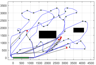
(a)

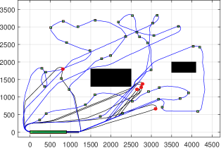
(b)

Figure 6: UAV mission with 10 UAVs and randomly distributed areas of interest (small green-coloured rectangles) in Section V. (a) Mission guidance by Algorithm 2. (b) Mission guidance by the comparison heuristic.

V-C4 Scenario with two UAVs

We consider the case where the UAV on the red-coloured trajectory in Fig. 5(a) must abruptly return to the airfield when being in the red-circled state in Fig. 5(b). At that time, the UAV on the blue-coloured trajectory is in the blue-circled state in Fig. 5(b) and shall take over all tasks. To this end, Algorithm 2 is applied to $S$, $g$, the remaining $38$ target sets and the indicated initial state. The parameter $\rho$ is chosen as $360$. The resulting trajectory is depicted in Fig. 5. If lines 15–23 in Algorithm 2 are skipped the resulting cost of the trajectory is $8\%$ higher than the optimized one. Nevertheless, in this scenario our heuristic proved weaker than the method based on the frequent evaluation of the value function. Runtimes and costs are given in Fig. 5(c).

V-C5 Scenario with 10 UAVs

While the number of target areas remains the same in this scenario, the number of UAVs increases to ten and the target sets are arranged much more diffuse. See Fig. 6. The error-free mission is computed by means of a VRP with 10 vehicles as constraint and infinite capacity. We let five UAVs be damaged at the red-circled states in Fig. 6 and apply Algorithm 2 and compare the results with the heuristic in Subsection V-C3. In this scenario Algorithm 2 proves more efficient. It provides controllers leading to a mission cost of $1994$ while for the naive solution it is $2023$.

VI Conclusions

The application of symbolic optimal control to vehicle mission guidance has been demonstrated for two types of missions. Following [6] we showed how to utilize the value functions of the underlying reach-avoid tasks and classical solvers for VRPs in order to heuristically reduce the overall mission cost (Section IV). Although symbolic optimal control is currently not suitable for missions with spontaneous changes in the specification due to high runtime requirements, we have given a possible direction towards dynamic controller adaptation (Section V).

References

- [1] G. B. Dantzig and J. H. Ramser, “The truck dispatching problem,” Management science, vol. 6, no. 1, pp. 80–91, 1959.
- [2] P. Toth and D. Vigo, The Vehicle Routing Problem, P. Toth and D. Vigo, Eds. Society for Industrial and Applied Mathematics, 2002.
- [3] R. P. Anderson and D. Milutinović, “The Dubins Traveling Salesperson Problem with stochastic dynamics,” in Dynamic Systems and Control Conference, vol. 2. Am. Society of Mech. Eng., Oct. 2013.
- [4] S. G. Manyam, S. Rathinam, and S. Darbha, “Computation of Lower Bounds for a Multiple Depot, Multiple Vehicle Routing Problem With Motion Constraints,” Journal of Dynamic Systems, Measurement, and Control, vol. 137, no. 9, 09 2015.
- [5] M. Mansouri, F. Lagriffoul, and F. Pecora, “Multi vehicle routing with nonholonomic constraints and dense dynamic obstacles,” in 2017 IEEE/RSJ International Conference on Intelligent Robots and Systems (IROS), 2017, pp. 3522–3529.
- [6] A. Weber and A. Knoll, “On the solution of the travelling salesman problem for nonlinear salesman dynamics using symbolic optimal control,” in Proc. European Control Conf. (ECC), Jun. 2021, pp. 1988–1994. [Online]. Available: http://arxiv.org/abs/2103.00260
- [7] J. Bellingham, M. Tillerson, A. Richards, and J. P. How, Multi-Task Allocation and Path Planning for Cooperating UAVs. Boston, MA: Springer US, 2003, pp. 23–41.
- [8] Y. Miao, L. Zhong, Y. Yin, C. Zou, and Z. Luo, “Research on dynamic task allocation for multiple unmanned aerial vehicles,” Trans. Institute of Measurement and Control, vol. 39, no. 4, pp. 466–474, 2017.
- [9] Z. Fu, Y. Mao, D. He, J. Yu, and G. Xie, “Secure multi-uav collaborative task allocation,” IEEE Access, vol. 7, pp. 35 579–35 587, 2019.
- [10] G. Reissig and M. Rungger, “Symbolic optimal control,” IEEE Trans. Automat. Control, vol. 64, no. 6, pp. 2224–2239, June 2019.
- [11] G. Reissig, A. Weber, and M. Rungger, “Feedback refinement relations for the synthesis of symbolic controllers,” IEEE Trans. Automat. Control, vol. 62, no. 4, pp. 1781–1796, Apr. 2017.
- [12] A. Weber and A. Knoll, “Approximately optimal controllers for quantitative two-phase reach-avoid problems on nonlinear systems,” in Proc. IEEE Conf. Decision and Control (CDC), 2020, pp. 430–437. [Online]. Available: http://arxiv.org/abs/2006.03862
- [13] G. Reissig and M. Rungger, “Abstraction-based solution of optimal stopping problems under uncertainty,” in Proc. IEEE Conf. Decision and Control (CDC). New York: IEEE, Dec 2013, pp. 3190–3196.
- [14] E. Macoveiciuc and G. Reissig, “Memory efficient symbolic solution of quantitative reach-avoid problems,” in Proc. American Control Conference (ACC). IEEE, July 2019, pp. 1671–1677.
- [15] A. Weber, M. Kreuzer, and A. Knoll, “A generalized Bellman-Ford algorithm for application in symbolic optimal control,” in Proc. European Control Conf. (ECC), May 2020, pp. 2007–2014. [Online]. Available: https://arxiv.org/abs/2001.06231
- [16] A. Girard and A. Eqtami, “Least-violating symbolic controller synthesis for safety, reachability and attractivity specifications,” Automatica, vol. 127, p. 109543, 2021.
- [17] M. Bellmore and S. Hong, “Transformation of multisalesman problem to the standard traveling salesman problem,” Journal of the ACM (JACM), vol. 21, no. 3, pp. 500–504, 1974.
- [18] K. Helsgaun, “An Extension of the Lin-Kernighan-Helsgaun TSP Solver for Constrained Traveling Salesman and Vehicle Routing Problems: Technical report,” Tech. Rep., 12 2017.
- [19] S. M. LaValle, Planning algorithms. Cambridge: Cambridge University Press, 2006.