AANG: Automating Auxiliary learniNG

Abstract

Auxiliary objectives, supplementary learning signals that are introduced to help aid learning on data-starved or highly complex end-tasks, are commonplace in machine learning. Whilst much work has been done to formulate useful auxiliary objectives, their construction is still an art which proceeds by slow and tedious hand-design. Intuition for how and when these objectives improve end-task performance has also had limited theoretical backing. In this work, we present an approach for automatically generating a suite of auxiliary objectives. We achieve this by deconstructing existing objectives within a novel unified taxonomy, identifying connections between them, and generating new ones based on the uncovered structure. Next, we theoretically formalize widely-held intuitions about how auxiliary learning improves generalization on the end-task. This leads us to a principled and efficient algorithm for searching the space of generated objectives to find those most useful to a specified end-task. With natural language processing (NLP) as our domain of study, we demonstrate that our automated auxiliary learning pipeline leads to strong improvements over competitive baselines across continued training experiments on a pre-trained model on 5 NLP tasks .

1 Introduction

Figure 1: We present the decomposition of some auxiliary objectives in NLP within our framework.

The auxiliary learning paradigm, where we augment a primary objective with extra learning signals to boost end-task performance, is a staple of many machine learning (ML) domains. In natural language processing (NLP), well known models like SpanBERT (Joshi et al., 2020) and RoBERTa (Liu et al., 2019b) are trained on masked language modelling (MLM) auxiliary objectives (Devlin et al., 2018) before fine-tuning on the end-task. And for speech processing and reinforcement learning (RL), Oord et al. (2018) introduced the popular contrastive predictive coding objective which achieved state of the art performance in many settings when multi-tasked with the end-task. Despite these successes and many more, research into devising such objectives has progressed in a very local, objective-by-objective manner (Raffel et al., 2019; Clark et al., 2020; Grill et al., 2020; Chen et al., 2020). Auxiliary objectives are constructed by hand-design and without much overarching structure, relying on the experience and intuition of a select group of researchers versed at making appropriate design choices. Unfortunately, this status-quo not only creates a technical barrier of entry for exploring auxiliary objectives in new domains but also, by virtue of its incremental nature, limits the rate at which new objectives are discovered and investigated.

To address the above challenges, this paper presents a framework for automatically generating and utilizing a large set of candidate auxiliary objectives. Our framework is seeded by the following key observation: leading auxiliary objectives across multiple domains can be viewed as making different design decisions within a 4 stage pipeline: Input Data $(\mathcal{D})\rightarrow$ Input Transformation $(\mathcal{T})\rightarrow$ Model Representation $(\mathcal{R})\rightarrow$ Output $(\mathcal{O})$. For instance, in RL, a common auxiliary objective is to predict the environment’s forward dynamics (Agrawal et al., 2016; Hafner et al., 2019). To construct this objective, the current task state-action pair $(\mathcal{D})$ is corrupted $(\mathcal{T})$ and then passed through the model to produce a latent representation $(\mathcal{R})$ which is finally used to predict the next state $(\mathcal{O})$. Similarly, in NLP, the XLNet (Yang et al., 2019) objective—which performs language modelling on a randomly factorized permutation of the input—can be written within our taxonomy as $\{\mathcal{D}$ = Out-of-Domain$,\mathcal{T}$ = No-op$,\mathcal{R}$ = Random-Factorized$,\mathcal{O}$ = Next Token$\}$. These two examples (along with others listed in Figure 1) fall within a class we term named objectives: objectives that have been previously proposed in the auxiliary learning literature.

Figure 2: Our framework in the context of NLP. We decompose named objectives within our four staged taxonomy : $\{\mathcal{D},\mathcal{T},\mathcal{R},\mathcal{O}\}$. By taking the cartesian product of choices across stages, we reproduce named objectives and discover new ones.

Decomposing named objectives within our taxonomy provides a unified view of the auxiliary learning landscape. From this vantage point, it becomes clear that there are many unexplored combinations of the various primitives used across named objectives. This presents a simple formula for automatically generating a large set of candidate objectives: take the cartesian product of the design decisions across given stages (Figure 2). Using this compositional process, not only can we reconstruct existing named objectives, we can also generate new combinations. This overcomes the tedium of implementing each objective independently since we can just reuse a small set of simple stage-wise primitives.

Generating a large set of objectives raises the natural question of how to efficiently select the most helpful ones for a given end task. Instead of leaving this to practitioner intuition, we develop principled guidelines to address this question by theoretically studying the impact of auxiliary learning on a particular end-task. Specifically, using arguments based on algorithmic stability (Hardt et al., 2016; Bousquet & Elisseeff, 2002), we derive end-task generalization error bounds that are dependent on the choice of auxiliary task. This contributes to existing theory (Saunshi et al., 2020; Xie et al., 2021) on how auxiliary learning impacts the end-task by suggesting a new candidate mechanism: auxiliary learning results in more stable optimization end-points in the sense of Bousquet & Elisseeff (2002), which in theory improves generalization of the final model.

Guided by our theory, we introduce AANG (Automating Auxiliary LearniNG), an efficient, structure-aware algorithm for adaptively combining a set of related objectives to improve generalization on a specific end-task. AANG incorporates the following prescriptions from our theory: (i) auxiliary tasks that are more similar to the end-task are desirable. Given a set of objectives, AANG learns adaptive weights to bring the composite objective closer to the end-task; (ii) in general, more auxiliary data is better. AANG maximizes the effective amount of data used in training by using all the generated objectives instead of taking task-specific subsets.

To empirically validate our method for automatically generating and utilizing auxiliary objectives, we experiment on five NLP tasks. We do so in the widely-used setting of continued pre-training (Gururangan et al., 2020; Aghajanyan et al., 2021; Dery et al., 2021b; Zhang et al., 2022), where a model trained with a single auxiliary objective on large-scale data is further trained on end-task related data. Without introducing any external data or architectural modifications, variants of AANG outperform strong and widely used baselines in 4 out of 5 tasks. AANG achieves an average improvement of $\mathbf{4.2\%}$ over standard fine-tuning of RoBERTa across our chosen tasks. We believe our results will spur further research into exploring automating auxiliary learning across a variety of settings. Notably, while we focus on NLP when discussing the space of auxiliary objectives (Section 3) and in our empirical evaluation (Section 6), our theoretical results (Section 4) and AANG itself are domain-agnostic.

2 Related Work

To properly scope this work, we define auxiliary learning as training a model on alternative objectives with the goal of improving performance on some primary end-task. Auxiliary learning is an instantiation of transfer learning (Caruana, 1997; Baxter, 2000; Ruder et al., 2019). It covers the pretrain-then-finetune paradigm (Huh et al., 2016; Devlin et al., 2018; Schneider et al., 2019; Gururangan et al., 2020) as well as end-task aware multitasking approaches (Lin et al., 2019; Dery et al., 2021a; b). Whilst auxiliary objectives may be meta-learned (Liu et al., 2019a; Navon et al., 2020), for simplicity – since incorporating these would require further complication of our design space – such objectives are out of the scope of this paper.

This work bears many parallels to the area of neural architecture search (NAS) (Stanley & Miikkulainen, 2002; Zoph & Le, 2016; Roberts et al., 2021). Whilst we seek to automate auxiliary learning, the objective of NAS is to automate the discovery of the right neural architecture given a specific end-task. Search spaces of candidate architectures are created by taking the cartesian product of architecture design choices across the depth of the network. The design of suitable architectural search spaces for a variety of settings has been an active area of research (Tan & Le, 2019; Howard et al., 2019; Dao et al., 2020; Roberts et al., 2021). To develop AANG, we borrow ideas from the NAS literature on efficient algorithms for sifting through spaces of architectures. Mirroring the popular differentiable NAS method DARTS Liu et al. (2018), we perform a continuous relaxation over the search space of objectives, allowing for efficient search by gradient descent. We also use a factored approach to model relationships between objectives that share primitives. This is inspired by recent work on stochastic-relaxation weight sharing (Dong & Yang, 2019; Li et al., 2020).

As a theoretical contribution, this work derives an end-task aware generalization error bound for auxiliary learning. Our bound is built on that of Hardt et al. (2016), who derive generalization bounds for parametric models trained with stochastic gradient descent (SGD). To derive their bounds, they leverage the concept of algorithmic stability introduced by Bousquet & Elisseeff (2002). Informally, a randomized algorithm is uniformly stable if changing a single training data point in the given samples does not change its end-point too much. Said change is characterized as the average difference in predictions between the two learned models. Stability implies generalization in expectation (Hardt et al., 2016; Kuzborskij & Lampert, 2018).

3 Automatically Generating Auxiliary Objectives

To begin, we take a high-level view of the landscape of named objectives. Using running examples from NLP, we propose the following coarse structure for the sequence of choices made in the hand-design of auxiliary objectives:

1. Data, $\mathcal{D}$: Auxiliary objective pipelines begin with a choice of input data. Here, options can range from heterogeneous out-of-domain data (Radford et al., 2019), in-domain data with respect to the final end-task (Beltagy et al., 2019) or the task data itself (Gururangan et al., 2020). It may even include data outside the modality of the end-task.

2. Input-Transformation, $\mathcal{T}$: Many auxiliary objectives are self-supervised with respect to their input data. They corrupt or transform the input and then reconstruct it in whole or part. For example, input text tokens can be masked, replaced or deleted. Operations can also be aggregated as in BERT-Op: mask 80% of selected tokens and randomly replace 50% of the remaining Devlin et al. (2018); Liu et al. (2019b).

3. Representation, $\mathcal{R}$: After transformation, representations of the input data can be computed from a given model in different ways. A chosen token’s representation can depend on only its left context (Left-to-Right) (Radford et al., 2018) or its right context (Right-to-Left) (Peters et al., 2018). It could also depend on the representations of a randomly selected permutation of other tokens (Random Factorized) Yang et al. (2019).

4. Output, $\mathcal{O}$: Finally, representations obtained from the previous stage are fed into a loss function producing a final output. The choice of output loss is usually coupled with the choice of transformation made in stage 2. Choices include but are not restricted to denoising tokens, predicting the next token or predicting the TF-IDF (Term Frequency-Inverse Document Frequency) of a token.

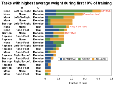
(a)

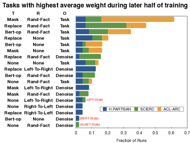
(b)

Figure 5: Top ranked objectives (averaged weight) early in training (left) and later in training (right)

The above taxonomy $\{\mathcal{D}\rightarrow\mathcal{T}\rightarrow\mathcal{R}\rightarrow\mathcal{O}\}$ is expansive enough to cover a range of named auxiliary objectives of interest in NLP (Figure 1). For example, we can write any member of the GPT series (Radford et al., 2018; 2019; Brown et al., 2020) which perform left-to-right language modelling on out-of-domain data as $\{\mathcal{D}$ = Out-of-Domain$,\mathcal{T}$ = No-op$,\mathcal{R}$ = Left-To-Right$,\mathcal{O}$ = Next Token$\}$. We can summarize the pre-existing choices within each design stage to obtain a unique set of options. For example, we can reduce the set of model representation types used by the objectives enumerated in Figure 1 to the unique set $\mathcal{R}=\{$Bi-directional, Left-To-Right, Right-To-Left, Random-Factorized$\}$. Having summarized the list of primitives within each stage, a simple formula for generating a space of auxiliary objectives becomes apparent: take the cartesian product of the design choices at each stage (see Figure 2). In general, given an instance of our taxonomy, we can construct a space of objectives $\mathcal{A}=\mathcal{D}\times\mathcal{T}\times\mathcal{R}\times\mathcal{O}$ of size $|\mathcal{A}|\leq|\mathcal{D}|\times|\mathcal{T}|\times|\mathcal{R}|\times|\mathcal{O}|$. Consider $\mathrm{New\_Obj}_{1}$ from Figure 2. This previously unexplored objective can be obtained by combining the special masking operation from BERT (BERT-Op) with computing model representations based on left-to-right causal masking as in GPT. In fact, this objective proved one of the most useful ones in our experiments below (see Figure 5).

Our framework also allows us to reason about whole families of objectives, $\mathcal{F}$, by thinking in terms of design stages and choices. For example, given a particular end-task $\mathbf{E}$ with input text $\mathbf{E}_{\mathcal{D}}$, we can create a family of objectives based solely on task data by fixing to that option in our input data stage; we call this family $\mathcal{F}_{\mathcal{D}=\mathbf{E}_{\mathcal{D}}}$. $\mathcal{F}_{\mathcal{D}=\mathbf{E}_{\mathcal{D}}}$ not only includes pre-existing TAPT Gururangan et al. (2020) but also unexplored objectives like task-data dependent variants of XLNET, ELMO etc. Auxiliary learning with $\mathcal{F}_{\mathcal{D}=\mathbf{E}_{\mathcal{D}}}$ can be seen as a relaxed form of data augmentation which we dub task augmentation. Whilst data augmentation requires applying transformations that preserve the data-point’s label, task augmentation has no such restriction and thus offers greater flexibility in terms of specifying $\{\mathcal{T},\mathcal{R},\mathcal{O}\}$. We can also reason about expanding particular stages to include new primitives. Any supervised loss can be added to the output stage, $\mathcal{O}$, allowing us to potentially explore auxiliary objectives based on supervised signals like NER or POS tagging (Carreras et al., 2003; Charniak, 1997). A special example is setting $\mathcal{O}$ to the end-task supervised output $\mathbf{E}_{\mathcal{O}}$. This leads to $\mathcal{F}^{\mathcal{O}=\mathbf{E}_{\mathcal{O}}}_{\mathcal{D}=\mathbf{E}_{\mathcal{D}}}$ which is a subset of $\mathcal{F}_{\mathcal{D}=\mathbf{E}_{\mathcal{D}}}$. $\mathcal{F}^{\mathcal{O}=\mathbf{E}_{\mathcal{O}}}_{\mathcal{D}=\mathbf{E}_{\mathcal{D}}}$ includes many objectives like predicting the end-task signal from corrupted input data. In Section 6, we will introduce a search space of objectives that leverages task augmentation.

4 The Impact of Auxiliary Learning on End-task Generalization

In this section, we relieve reliance on practitioner intuition by deriving a set of guiding principles on how to effectively utilize the automatically generated objectives from Section 3.

Auxiliary learning influences the end-task through both training and generalization error. Previous theory has largely focused on characterizing the impact on end-task training error. Liu et al. (2021), for example, show that end-task agnostic pre-training can create a performance gap in training error compared to training with the end-task alone. The size of this gap depends on how dissimilar the pre-training auxiliary objective is from the end-task. They introduce the following assumption (which we will borrow) to formalize their notion of task similarity:
Assumption A.1: Let $f_{e}$ represent the end-task objective and $f_{a}$ be the auxiliary objective. There exists $\Delta\geq 0$ such that $\|\nabla f_{a}(\theta)-\nabla f_{e}(\theta)\|\leq\Delta\leavevmode\nobreak\ \leavevmode\nobreak\ \forall\leavevmode\nobreak\ \theta$.
Note that $\theta$ represents all the parameters of the model. Smaller $\Delta$ implies $f_{a}$ is more similar to the primary task $f_{e}$. Liu et al. (2021) bound the end-task agnostic training error gap to be logarithmic in $\Delta$.

Unlike training error, end-task generalization error has gone unstudied in the auxiliary learning setting. Bounding the generalization error not only adds to our theoretical understanding of the impact of auxiliary learning but also provides insights to guide algorithm design. To arrive at a bound, we adapt the technique of Hardt et al. (2016) who derive a generalization bound on training with only the end-task via stochastic gradient descent. We consider the end-task aware setting where the end-task is multi-tasked with the auxiliary objective. This setting has recently been shown to improve end-task performance over the pretrain-then-finetune paradigm (Dery et al., 2021a; b; Yao et al., 2021).

Auxiliary learning with Dynamic Sampling: We are given an auxiliary objective $f_{a}(\cdot;z)\in[0,1]$ with $N_{a}$ samples $S_{a}=(z_{1},\ldots,z_{N_{a}})$ from the distribution $\mathcal{D}_{a}$. $f_{a}$ can either be a single objective or a weighted linear combination of objectives : $f_{a}=\sum_{k}w^{k}f^{k}_{a}$. At any iteration of SGD, we sample a choice of the end-task function $f_{e}$ or the auxiliary objective $f_{a}$ according to the probabilities $\lambda_{e}$, $\lambda_{a}\in[0,1]\leavevmode\nobreak\ |\leavevmode\nobreak\ \lambda_{e}$ + $\lambda_{a}=1$. Given the chosen objective, we sample a data-point and perform stochastic gradient descent based on the sampled data-point. We now present our bound in the setting described.

Theorem 4.1 (Auxiliary learning with Dynamic Sampling).

Assume that $f_{e}(\textperiodcentered;z_{e}),f_{a}(\textperiodcentered;z_{a})\in[0,1]$ are both $L$-Lipschitz with $\beta_{e}$ and $\beta_{a}$-smooth loss functions respectively. Consider that we have $N^{\prime}=N_{e}+N_{a}$ total samples where $f_{e}$ and $f_{a}$ have $N_{e}$ and $N_{a}$ samples respectively. $r_{e}=\frac{N_{e}}{N^{\prime}}$ is the fraction of the available data represented by the end-task. Suppose that we run stochastic gradient descent for T steps with monotonically non-increasing step sizes $\alpha_{t}\leq\frac{c}{t}$ by dynamically sampling the tasks according to $\lambda_{e}$ and $\lambda_{a}$. Then, with respect to $f_{e}$, the generalization error is bounded by:

$$\epsilon_{\mathrm{gen}}\leavevmode\nobreak\ \lessapprox\leavevmode\nobreak\ \big{(}\Delta)^{\frac{1}{1+c\lambda^{*}\beta^{*}}}\bigg{(}\frac{\gamma T}{N^{\prime}}\bigg{)}^{1-\frac{1}{c\lambda^{*}\beta^{*}+1}}\quad\text{Where}\quad\gamma=\frac{\lambda_{e}}{r_{e}}$$ (1)

Here $\beta^{*}=\min\{\beta_{e},\beta_{a}\}$ and $\lambda^{*}$ is the weighting of the function with smaller smoothness.

Proof.

See Appendix E for full proof and Appendix F for more discussion ∎

As a detailed inspection of the proof will show, we derive Equation 1 by appealing to algorithmic stability (Bousquet & Elisseeff, 2002; Hardt et al., 2016; Kuzborskij & Lampert, 2018) (Section 2). To our knowledge, ours is the first work to present an algorithmic stability view to formally explain how auxiliary learning influences end-task performance. Equation 1 surfaces the following prescriptions about learning with auxiliary tasks :

1. Smaller $\Delta$ improves $\epsilon_{\mathrm{gen}}$. This implies that the more similar the auxiliary objective is to the end-task (under Assumption A.1), the lower the generalization error.

2. Larger $N^{\prime}$ leads to smaller $\epsilon_{\mathrm{gen}}$. Since we usually have a fixed amount of task data $N_{e}$, we can increase $N^{\prime}$ by adding more auxiliary data $N_{a}$.

Algorithm 1 AANG

  Input: Search Space - $\mathcal{A}$Factor vectors - $\{W^{\mathrm{All}},W^{\mathcal{I}},W^{\mathcal{T}},W^{\mathcal{R}},W^{\mathcal{O}}\}$End-task - $\mathbf{E}$, End-task weight - $\lambda_{e}$Initial Model Params - $\theta_{0}\in\mathbf{R}^{D}$

  repeat

      Sample a batch of $n$ objectives$\mathcal{K}^{n}\sim\mathcal{A}$ Weighting of objectives in $\mathcal{K}^{n}$

     Construct $\mathbf{w}^{n}$

     for $k=1$ to $n$ do

        $(d,\leavevmode\nobreak\ t,\leavevmode\nobreak\ r,\leavevmode\nobreak\ o)=[\mathcal{K}^{n}_{k}]\mathrm{.stages}$

        $w^{k}\propto\exp\big{(}W^{\mathrm{All}}_{(d,\leavevmode\nobreak\ t,\leavevmode\nobreak\ r,\leavevmode\nobreak\ o)}+W^{\mathcal{I}}_{d}+W^{\mathcal{T}}_{t}+W^{\mathcal{R}}_{r}+W^{\mathcal{O}}_{o}\big{)}$

        $\mathbf{w}^{n}_{k}\leftarrow w^{k}$

     end for

      Get losses from batches of data$\hat{\mathcal{L}}_{\mathcal{A}}(\mathcal{K}^{n},\mathbf{w}^{n})=\sum^{n}_{k=1}w^{k}\mathcal{L}_{k}$ $\mathcal{L}_{\mathrm{total}}=\lambda_{e}\mathcal{L}_{E}+(1-\lambda_{e})\hat{\mathcal{L}}_{\mathcal{A}}$ Get gradients and update factors$\theta_{t+1},\{\nabla_{\mathbf{w}^{n},\lambda_{e}}\}\leftarrow$ META-TARTAN$\big{(}\theta_{t},E,\mathcal{L}_{\mathrm{total}})$ Update $\{W^{\mathrm{All}},W^{\mathcal{I}},W^{\mathcal{T}},W^{\mathcal{R}},W^{\mathcal{O}}\}$ using ${\nabla_{\mathbf{w}^{n}}}$ Update $\lambda_{e}$ using $\nabla_{\lambda_{e}}$

  until done

  Return : $\theta_{T}$

5 End-task Aware Search of Structured Objective Spaces

Guided by Section 4, we build a practical method for exploring a set of objectives, $\mathcal{A}$.

Whilst the dynamic sampling setting described in Section 4 is amenable to theoretical consideration, we make a few practical changes to it. First, instead of performing alternating gradient descent by sampling $f_{a},f_{e}$ according to $\lambda_{e},\lambda_{a}$, we instead use them as multitask weights and perform joint training. Joint training has been found to produce superior results compared to alternating optimization when leveraging auxiliary objectives (Aghajanyan et al., 2021). We perform gradient descent on the following total loss which interpolates between the end-task and the auxiliary loss $\mathcal{L}_{\mathrm{total}}=\lambda_{e}\mathcal{L}_{E}+(1-\lambda_{e})\mathcal{L}_{\mathcal{K}}$. Here, $\mathcal{K}$ is a chosen subset of $\mathcal{A}$.

Second, as indicated in Section 4, given $\mathcal{K}$, we can write the set as a single objective $f_{a}=\sum_{k\in\mathcal{K}}w^{k}f^{k}_{a}$. By Prescription ($P_{1}$), we want to choose $\{w^{k}\}$ such that $f_{a}$ has a small $\Delta$ with the end-task $f_{e}$. We would also like to set $\lambda_{e}$ such that the bound on $\epsilon_{\mathrm{gen}}$ is minimized. Whilst a closed form exists for the optimal weightings $\lambda_{e},\{w^{k}\}$, it depends on variables like $\{\Delta^{k}\},\{\beta^{k}_{a}\},L$ that are hard to estimate. We therefore propose to learn $\lambda_{e},\{w^{k}\}$ in an online, data-driven way. To do this, we build on top of the META-TARTAN algorithm proposed by Dery et al. (2021b). META-TARTAN is a meta-learning algorithm that learns adaptive weights for different auxiliary tasks in a way that prioritizes end-task generalization. It learns $\{w^{k}\}$ by minimizing the loss on the end-task validation set: $\frac{\partial\mathcal{L}^{val}_{\mathbf{E}}}{\partial w^{k}}\approx-\big{(}\nabla_{\theta}\mathcal{L}_{f_{a}^{k}}\big{)}^{T}\big{(}\nabla_{\theta}\mathcal{L}^{val}_{\mathbf{E}}\big{)}$. This corresponds to learning $\{w^{k}\}$ such that $\big{(}\nabla_{\theta}f_{a}\big{)}^{T}\big{(}\nabla_{\theta}f_{e})$ is maximized. This minimizes one of the terms that contributes to $\Delta$ and thus attempts to fulfil Prescription ($P_{1}$). We can similarly learn $\lambda_{e}$ to minimize the end-task validation loss. For a more detailed discussion of META-TARTAN, please see Appendix B.

So far, we have introduced independent weights, $\{w^{k}\}$, for each objective. This is sufficient in the case of unrelated objectives. However, the objectives in $\mathcal{A}$ share an underlying structure. We recognize this by using a factored approach to model each $w^{k}$. We introduce a factor vector for each of the 4 stages introduced in Section 3: $W^{\mathcal{D}}\in\mathbf{R}^{|\mathcal{D}|},W^{\mathcal{T}}\in\mathbf{R}^{|\mathcal{T}|},W^{\mathcal{R}}\in\mathbf{R}^{|\mathcal{R}|}$ and $W^{\mathcal{O}}\in\mathbf{R}^{|\mathcal{O}|}$. This ties together the weights of objectives that share primitives in common. To capture the fact that an objective can be more than the sum of it parts, we also introduce an independent weight for each objective : $W^{\mathrm{All}}\in\mathbf{R}^{|\mathcal{D}|\times|\mathcal{T}|\times|\mathcal{R}|\times|\mathcal{O}|}$. Consider the objective $k$ which is generated by the composition of the operations $\{d\in\mathcal{D},\leavevmode\nobreak\ t\in\mathcal{T},\leavevmode\nobreak\ r\in\mathcal{R},\leavevmode\nobreak\ o\in\mathcal{O}\}$, its weighting is computed as : $w^{k}\propto\exp\big{(}W^{\mathrm{All}}_{(d,t,r,o)}+W^{\mathcal{I}}_{d}+W^{\mathcal{T}}_{t}+W^{\mathcal{R}}_{r}+W^{\mathcal{O}}_{o}\big{)}$. Our factored approach not only allows us to share information between objectives but it also allows us to analyze which stages and primitives are most important to a particular end-task after training is completed (Section 7).

Prescription 4 from Section 4, advocates for introducing as much auxiliary data as possible. As such, instead of fixing to a specific subset throughout training for a particular end-task, we propose to utilize all the objectives in $\mathcal{A}$. This also avoids the combinatorial explosion that comes with exploring subsets of $\mathcal{A}$ at a time. $|\mathcal{A}|$ can be large and descending on all of $\mathcal{A}$ at once can be computationally prohibitive. As an efficient work around, at each training step, we sample a subset of $\mathcal{A}$ for execution with META-TARTAN. Our samples are drawn from all of $\mathcal{A}$ so any objective can get used at any timestep. Because we model each $w^{k}$ via a factored approach, even if an objective is not sampled its weight is implicitly updated. Our approach is reminiscent of stochastic-relaxation weight sharing (Pham et al., 2018; Dong & Yang, 2019; Li et al., 2020) where sampled architectural primitives result in updates to shared model weights which can be used by other primitives that are not sampled.

We coalesce all the ideas we have introduced so far into Algorithm 1 which we dub AANG  (Automated Auxiliary LearniNG). At a high-level, given an end-task $\mathbf{E}$:

1. We generate a space of auxiliary objectives $\mathcal{A}$ by leveraging the taxonomy discussed in Section 3. $\mathcal{A}$ may contain auxiliary tasks that can improve our performance on $\mathbf{E}$.

2. We leverage MAML-style (Finn et al., 2017) meta-learning to adaptively weight the objectives in $\mathcal{A}$ based on measuring each objective’s influence on $\mathbf{E}$’s validation set loss.

3. We make our algorithm scalable by sub-sampling the tasks $\mathcal{A}$. By exploiting the underlying structure of the objectives in $\mathcal{A}$ via a factored approach to modeling task weights, we reduce the impact of the inexact sub-sampling.

6 Experimental Setting

Our exploration of auxiliary learning has made the following transitions from the status-quo: manual to automated, single task to multitask, end-task agnostic to end-task aware. In this section, we set up experiments to validate these deviations from the standard.

We focus on continued pre-training (Gururangan et al., 2020; Aghajanyan et al., 2021). In this setting, we perform further auxiliary learning on an already pre-trained model. We favor this setting over pre-training from scratch (Liu et al., 2019b; Yang et al., 2019) not only because it is a more computationally feasible arena for experimentation but also because it is more relevant to modern ML systems where building upon pre-trained models is the norm (Qiu et al., 2020; Du et al., 2020).
Model Details and Datasets:  We use a pre-trained RoBERTa_base (Liu et al., 2019b) as the shared model base. We implement each auxiliary objective as a separate head on top of this shared base. For classification based objectives, the output head is a 2-layer multi-layer perceptron (MLP) that receives representations for the special classification token [CLS] (Devlin et al., 2018) from RoBERTa_base. For sequence generation objectives, we make a copy of the pre-trained output layer of RoBERTa_base for each task. Table 4 in Appendix C provides details of the 5 datasets used. All datasets are low-resource classification tasks. Not only are these datasets more amenable to meta-learning from a computational standpoint, but low-resource tasks also benefit the most from auxiliary learning. We also choose these tasks because they feature in previous work which we use as baselines (Gururangan et al., 2020; Dery et al., 2021b)
Baselines and Search Spaces: The following methods are end-task agnostic baselines. By end-task agnostic, we mean that these do not multitask with the end-task. Finetuning on the end-task occurs after training on the auxiliary objective.

1. RoBERTa (Liu et al., 2019b): We simply finetune a pre-trained RoBERTa_base on the end-task.

2. TAPT (Gururangan et al., 2020): Continue training RoBERTa_base on masked language modelling on end-task data itself before finetuning on the end-task.

The following named objectives are end-task aware baselines that use META-TARTAN (Dery et al., 2021b) but utilize only 1 auxiliary task. Each auxiliary objective is multi-tasked with the end-task.

1. GPT-style: We perform end-task aware training with a denoising auxiliary objective based on left-to-right causal masking for computing representations. {$\mathcal{I}$ = End-task data, $\mathcal{T}$ = No-op, $\mathcal{R}$ = Left-To-Right, $\mathcal{O}$ = Denoise Token }.

2. XLNET-style: This is a denoising auxiliary objective that uses randomized masking for computing representations. {$\mathcal{I}$ = End-task data, $\mathcal{T}$ = No-op, $\mathcal{R}$ = Random-factorized, $\mathcal{O}$ = Denoise Token}.

3. BERT-style / TAPT: Denoising inputs corrupted via BERT-Op: 80% masking and 10% random replacement. {$\mathcal{I}$ = End-task data, $\mathcal{T}$ = BERT-Op, $\mathcal{R}$ = Bi-directional, $\mathcal{O}$ = Denoise Token}. Please note that this baseline is equivalent to META-TARTAN as introduced in Dery et al. (2021b).

Table 1: AANG-TD (task data) has 24 objectives and is based on only end-task data. AANG-TD+ED (task data + external data) has 40 objectives and uses both end-task and in-domain data.

	$\mathcal{I}$	$\mathcal{T}$	$\mathcal{R}$	$\mathcal{O}$
TD	End-task	BERT-op	Bi-directional	Denoise Token
		Mask	Left-to-Right	End-task
TD+ED	End-task	Replace	Right-to-Left
	In-Domain data	No-op	Random-Factorized

Table 1 details the search spaces that we evaluate against the above baselines. This is by no means the most encompassing search space but we leave more expansive space design to future work. Please note that all tasks within AANG-TD, and those with $\{\mathcal{I}=$ End-task$\}$ in AANG-TD+ED, are instantiations of task augmentation as introduced in Section 3.
Training Details : Please see Appendix D for more details about hyper-parameter configurations.

7 Results and Discussion

In this section, we experimentally validate our case for automating the creation of auxiliary objectives and using them in an end-task aware multitask fashion.

7.1 Going a Long Way Without External Data

We first consider the setting where we rely solely on end-task data (task augmentation), and work with the AANG-TD search space. This search space has 24 objectives. Table 2 shows that automatically generating auxiliary objectives from only task data and using them appropriately is productive.
End-task awareness is key: From Table 2, methods that are end-task aware result in over $1.12\%$ average improvement over those that are end-task agnostic even under the most generous comparison (GPT-style $79.84\%$ vs task-agnostic TAPT $78.72\%$). Knowing the end-task means that at each iteration, AANG can make informed gradient updates by adapting task weights so the resulting auxiliary task better aligns with the end-task (Prescription ($P_{1}$)). Amongst the single task objectives, BERT-style performs best. We posit that this is because RoBERTa was trained from scratch on a similar objective and so this objective represents minimal shift in training distributions.

Table 2: Our framework and AANG on tasks using only task data. Without using any external data, we are able to get significant average performance improvement over baselines. Superscripts are p-values from paired t-tests (best multitask versus best single-task).

Task Adaptive	Method	#	CS		BIOMED	NEWS	STANCE
			ACL-ARC	SCIERC	CHEMPROT	H.PARTISAN	SE-2016-6	AVG
No	RoBERTa	1	$66.03_{3.55}$	$77.96_{2.96}$	$82.10_{0.98}$	$93.39_{2.26}$	$70.37_{1.51}$	$77.97$
	TAPT	1	$67.74_{3.68}$	$79.53_{1.93}$	$82.17_{0.65}$	$93.42_{2.87}$	$70.74_{1.21}$	$78.72$
	[OURS] Static Multitask-TD	24	$69.60_{3.80}$	$\mathbf{83.37}_{0.58}$	$83.42_{0.26}$	$97.95_{0.73}$	$71.02_{0.43}$	$81.07$
Yes	X. GPT-style	1	$67.22_{0.44}$	$81.62_{0.84}$	$83.29_{1.21}$	$96.41_{0.73}$	$70.67_{1.46}$	$79.84$
	Y. XLNET-style	1	$69.76_{2.42}$	$81.81_{0.42}$	$83.39_{0.31}$	$96.41_{1.92}$	$71.18_{0.58}$	$80.51$
	Z. BERT-style (Dery et al., 2021b)	1	$70.08_{4.70}$	$81.48_{0.82}$	$\bm{84.49}_{0.50}^{{\color[rgb]{0,0,1}(0.09)}}$	$96.84_{1.72}$	$72.70_{0.60}$	$81.12$
	[OURS] AANG-[X+Y+Z]	3	$71.51_{3.19}$	$82.89_{0.78}$	$83.68_{0.45}$	$96.92_{1.26}$	$\bm{72.75}_{0.82}^{{\color[rgb]{1,0,0}(0.94)}}$	81.55
	[OURS] AANG-TD	24	$\bm{73.26}_{1.32}^{{\color[rgb]{0,0,1}(0.28)}}$	$\bm{82.98}_{1.52}^{{\color[rgb]{0,0,1}(0.27)}}$	$83.91_{0.32}$	$\bm{98.46}_{0.0}^{{\color[rgb]{0,0,1}(0.14)}}$	$72.46_{1.65}$	$\mathbf{82.21}$

Adaptive multi-task auxiliary learning improves performance: We compare single-task end-task aware auxiliary learning to its multitask variant. Table 2 shows that multitasking our 3 different types of language modelling tasks results in improved average performance over using the tasks individually (81.12% for the BERT-style and 81.55% for combining the three single task objectives). We get our best performance when we multitask 24 auxiliary objectives automatically generated with our framework using AANG-TD. Boosting the number of objectives from 3 to 24 resulted in a 0.66% improvement in average performance across tasks. This is in line with Prescription 4 from Section 4 since we are increasing the effective amount of auxiliary data. We further posit that introducing more auxiliary objectives also serves to implicitly regularize the end-task during training.

7.2 Introducing External Data

Figure 3: AANG effectively leverages out-of-task data. P-values (in brackets) are comparisons to (Dery et al., 2021b)

For the ACL-ARC task, we experiment with introducing auxiliary tasks based on external data. AANG-TD+ED has 40 tasks, 16 of which are based on domain data. We introduce CS domain data (from the S2ORC dataset (Lo et al., 2019)) that is $n=10\times$ the size of the task data. From Figure 3 we see that AANG-TD+ED makes better use of domain-data than doing end-task aware training using only BERT-style objective with task (TAPT) and domain-data (DAPT) jointly as in Dery et al. (2021b). However, AANG-TD+ED ($73.70$) does not significantly improve over AANG-TD ($73.26$) on the ACL-ARC task (Figure 3). This might seem at odds with Prescription 4 since the TD+ED search space introduces more data. However, note that the AANG search algorithm is approximate and as such, with a larger search space, it can be harder to find composite tasks with a small $\Delta$ as suggested by Prescription ($P_{1}$). We posit that we need more external data than $n=10\times$ in order to see marked improvements to offset our inexact search of the space of composite functions. However, such scales are outside our computational budget.

7.3 Why does AANG Work ?

To better understand why our auxiliary learning pipeline improves end-task performance, we perform multiple ablations under AANG-TD.
Static versus Dynamic Weighting: We ablate the impact of using static task weights throughout training, as against adaptive task weights. Just as with AANG, we sub-sample $n$ tasks from the search space at every iteration ($n$ is cross-validated exactly as AANG is – Table 5 ). Each sampled tasks weight is initialized to $\frac{1}{n}$ and this remains unchanged throughout training. This is the Static Multitask-TD baseline in Table2. AANG-TD improves upon the static multitask baseline by over 1.1% on average. With adaptive weighting, AANG down-weights objectives that are harmful to the end-task whilst up-weighting relevant ones (Prescription ($P_{1}$)). However, using static weightings is more compute friendly since we do not have to calculate task-weight meta-gradients. This compute-vs-performance trade-off is left for practitioners to resolve based on their available resources.
Impact of number of sampled objectives: Due to computational constraints, AANG sub-samples the set of generated objectives. Whilst this sampling can result in approximation error when inferring task weightings, it can also introduce stochasticity which can help regularize the learned model. From Table 3 (Appendix A) we find that for some tasks (ACL-ARC and SCIERC) sampling a larger number of tasks helps. SE-2016-6 and CHEMPROT on the other hand benefit from smaller number of sampled tasks. Our recommendation is that the number of sampled tasks be cross-validated on a per-task basis.
Learned task weight trajectories: AANG learns interesting trajectories for weighting design stage primitives. From Table 2, the fact that AANG-TD roughly matches the best single task performance ($72.46_{1.65}$ versus $72.70_{0.60}$ for BERT-style) on the SE-2016-6 task suggests that it may be learning to mostly up-weight this task. Figure 4 provides evidence of this. For the SE-2016-6 task (row 1), composing the highest weighted primitive from each stage [BERT $\circ$ None $\circ$ DENOISE] results in BERT-style, the best single task objective. Figure 4 also shows that AANG can adapt to overfitting. The vertical black lines indicate the point of best validation set performance. AANG responds to over-fitting by down-weighting objectives based on the output loss being over-fit to. Thus, after several iterations, the objective that dominates when the validation performance is at its highest (black vertical line) gets down-weighted in response to it becoming saturated.

Figure 4: Learned trajectories for AANG-TD for run instances of SE-2016-6 and SCIERC tasks.

What tasks are important and when they are important? We study which tasks are most highly weighted early in training (first 10% of learning trajectory) and later in training (last 50%). We aggregate statistics across 3 datasets.

Note that early in training, objectives based on the self-supervised output $\mathcal{O}=$ {DENOISE} are highly weighted but later, objectives based on supervised signal, $\mathcal{O}=$ {Task} play a larger role. AANG rediscovers the common practice of training on self-supervised objectives before introducing supervised ones. It is also interesting to note that many newly generated objectives (outside of the 3 named single task baselines in Table 2) such as simple input reconstruction were discovered to have relevant impact on the end-tasks. This means AANG can automatically surface new, previously unexplored objectives relevant to the end-task.

8 Limitations and Conclusion

Our work has some limitations that we leave for future work. First, because AANG relies on meta-learning, it presents extra compute burden over simple multitasking. This is because, we have to independently compute meta-gradients for each auxiliary task thus requiring $\mathcal{O}(n)$ forward-backward operations for $n$ sampled tasks compared to $\mathcal{O}(1)$ for static multitasking. In Table 2, we show that our static Multitask-TD method outperforms all other non-task-adaptive methods by $\approx 2.4\%$ and is thus a viable alternative when runtime is a signficant constraint. Secondly, AANG as presented is an approximate algorithm – primarily due to sub-sampling the space of tasks. Thus as mentioned in Section 7.2, we do not get as much gain as desired when our search space becomes larger. We leave finding an efficient exact search algorithm for future exploration.

This paper presents a procedure for automating the creation of auxiliary objectives. We showed, theoretically, how auxiliary learning impacts end-task generalization. This resulted in prescriptions that informed the design of AANG, an algorithm to search the space of generated objectives in an end-task aware multitask fashion. Our experiments show that AANG is a promising first step in automating auxiliary learning.

9 Acknowledgements

This work was supported in part by DSO National Laboratories, an ENS-CFM Data Science Chair, DARPA FA875017C0141, the National Science Foundation grants IIS1705121, IIS1838017, IIS2046613 and IIS-2112471, an Amazon Web Services Award, a Facebook Faculty Research Award, funding from Booz Allen Hamilton Inc., and a Block Center Grant. Any opinions, findings and conclusions or recommendations expressed in this material are those of the author(s) and do not necessarily reflect the views of any of these funding agencies. We are grateful for helpful feedback from Uri Alon, Patrick Fernandes, Joon Sik Kim, Han Guo, Victor Akinwande and Clara Na.

Appendix A More Ablation Tables

Table 3: Varying number of sampled objectives per-iteration.

Task	$\frac{3}{24}$ tasks	$\frac{6}{24}$ tasks
ACL-ARC	$72.11_{2.12}$	$\mathbf{73.26}_{1.32}$
SCIERC	$82.35_{1.76}$	$\mathbf{82.98}_{1.52}$
SE-2016-6	$\mathbf{72.46}_{1.65}$	$\mathbf{72.46}_{0.90}$
CHEMPROT	$\mathbf{83.91}_{0.32}$	$83.69_{0.98}$
H.PARTISAN	$\mathbf{98.46}_{0.0}$	$97.95_{0.73}$

Appendix B Discussion of META-TARTAN (Dery et al., 2021b)

META-TARTAN (Dery et al., 2021b) is a MAML style (Finn et al., 2017) meta-learning algorithm that learns to adaptively weight a given set of tasks based on their influence on the end-task validation performance. META-TARTAN achieves this by formulating the following bi-level optimization problem :

$$\theta^{*},\mathbf{w}^{*}=\mathrm{argmin}_{\{\theta\leavevmode\nobreak\ \in\leavevmode\nobreak\ g(\theta_{0}),\leavevmode\nobreak\ \mathbf{w}\}}\leavevmode\nobreak\ \mathcal{L}_{\mathbf{E}}(\theta)$$ (2)

where

$$\begin{split}\theta_{0}&=\mathrm{argmin}_{\theta}\leavevmode\nobreak\ \leavevmode\nobreak\ \mathcal{L}_{\mathrm{total}}(\theta,\mathbf{w})=\mathrm{argmin}_{\theta}\leavevmode\nobreak\ \leavevmode\nobreak\ \bigg{(}w^{*}\mathcal{L}_{\mathbf{E}}(\theta)\leavevmode\nobreak\ +\sum_{T_{i}\in\mathcal{A}}w_{i}\mathcal{L}_{T_{i}}(\theta)\bigg{)}\end{split}$$ (3)

Note that $\mathbf{E}$ is the end-task and $\mathcal{A}$ is the set of auxiliary tasks.

Since the above bi-level problem is difficult to solve directly, Dery et al. (2021a) relax the problem and into an alternating optimization problem where task weights are updated based on 1-step improvement to the validation performance of the end-task :

$$\frac{\partial\mathcal{L}^{val}_{\mathbf{E}}(\theta_{t+1}(\mathbf{w}))}{\partial w_{i}}\approx-\beta\big{(}\nabla\mathcal{L}_{T_{i}}\big{)}^{T}\big{(}\nabla\mathcal{L}^{val}_{\mathbf{E}}(\theta_{t})\big{)}$$ (4)

To prevent the above relaxation from finding the trivial solution of just upweigting solely the end-task, Dery et al. (2021b) introduce a special dev-head which they use for estimating the meta-gradient :

$$\frac{\partial\mathcal{L}^{val}_{T^{*}}(\theta^{*}(\mathbf{w}))}{\partial w_{i}}\approx-\beta\big{(}\nabla_{\theta}\mathcal{L}_{T_{i}}\big{)}^{T}\big{(}\nabla_{\theta}\mathcal{L}^{val}_{\mathbf{E}}([\theta_{\mathrm{body}};\phi^{*}]_{t})\big{)}$$ (5)

Where $\phi^{*}_{t}$ is the special dev-head and $\theta_{\mathrm{body}}$ is the body of the model. For even more details about META-TARTAN, please see Section 3 of Dery et al. (2021b).
Though we leverage MET-TARTAN, compared to Dery et al. (2021b), we make three distinct contributions to the field of auxiliary learning. We list them below

1. Novel Problem Formulation: As far as we are aware of, we are the first to formulate the problem of automated auxiliary learning. Specifically, we presented an approach for automatically constructing a suite of auxiliary objectives based on existing objectives. Please note that Dery et al. (2021b) perform auxiliary learning with only the DAPT/TAPT variants of the BERT objective. They effectively assume that the search space of objectives (the 2 they explore) is given before-hand. Our approach automatically creates the search space.

2. Theoretical Novelty: To the best of our knowledge, we are the first work to provide an exploration of why auxiliary learning improves primary task performance via algorithmic stability. Dery et al. (2021b) in introducing META-TARTAN do not attempt to give a theoretical characterization of why the algorithm improves end-task performance.

3. Algorithm Improvements to META-TARTAN: Please note that META-TARAN as presented in Dery et al. (2021b) was used with only 2 auxiliary tasks. When scaling to more tasks, using META-TARTAN naively becomes computationally prohibitive. Specifically, on a search space of N tasks, META-TARTAN requires $O(N)$ order computation per step. We improve upon this by introducing the task sub-sampling of ($k\ll N$) which reduces the compute overhead to $O(k)$. To account for the impact of sub-sampling as an approximation, we introduced the factorised modelling of task weights which allows sharing of information between auxiliary tasks that might themselves be related.

Appendix C Dataset Details

Table 4: Specifications of datasets used to evaluate our methods.

Domain	Task	Label Type	Train Size	Dev Size	Test Size	Classes	Metric
BIOMED	CHEMPROT Kringelum et al. (2016)	relation classification	4169	2427	3469	13	Accuracy
CS	SCIERC Luan et al. (2018)	relation classification	3219	455	974	7	F1
STANCE	SE-2016-6 Mohammad et al. (2016)	stance detection	2497	417	1249	3	Accuracy
CS	ACL-ARC Jurgens et al. (2018)	citation intent	1688	114	139	6	F1
NEWS	H.PARTISAN Kiesel et al. (2019)	partisanship	515	65	65	2	Accuracy

Appendix D More Training Details

We run each hyper-parameter configuration across 3 seeds {0, 1, 2}. We use a batch size of 128 for all end-tasks tasks except H.PARTISAN where we use a batch size of 64. The auxiliary task batch-size, aux_bsz, is shared across all the $n$ sub-sampled auxiliary objectives according to the objective’s weight.

We use the AdamW optimizer (Loshchilov & Hutter, 2017), with weight decay of 0.01 for all experiments.

Table 5: AANG-TD specific Hyper-parameters

Hyper-parameter	Values	Description
aux_lr	1.0, 0.1	Learning rate for factor vectors - $\{W^{\mathrm{All}},W^{\mathcal{I}},W^{\mathcal{T}},W^{\mathcal{R}},W^{\mathcal{O}}\}$
sopt_lr	0.1, 0.01	Learning rate for primary task weighting $\lambda_{e}$
nconf_subsamp	3, 6	Number of sub-sampled auxiliary tasks.
learning rate	1e-3, 1e-4	Learning rate used for further training of RoBERTabase
aux_bsz	256	Batch size of for auxiliary objectives

Table 6: AANG-TD+ED specific Hyper-parameters

Hyper-parameter	Values	Description
aux_lr	1.0, 0.5, 0.1	Learning rate for factor vectors - $\{W^{\mathrm{All}},W^{\mathcal{I}},W^{\mathcal{T}},W^{\mathcal{R}},W^{\mathcal{O}}\}$
sopt_lr	0.1	Learning rate for primary task weighting $\lambda_{e}$
nconf_subsamp	6, 12, 24	Number of sub-sampled auxiliary tasks.
learning rate	1e-4	Learning rate used for further training of RoBERTabase
aux_bsz	1024	Batch size of for auxiliary objectives

Table 7: META-TARTAN Hyper-parameters for single task auxiliary tasks

Hyper-parameter	Values	Description
sopt_lr	1.0, 0.1, 0.01	Learning rate for primary task weighting $\lambda_{e}$
learning rate	1e-3, 1e-4, 5e-5	Learning rate used for further training of RoBERTabase

META-TARTAN introduces a dev-head which is trained sporadically during training for estimating the meta-gradients. We use the following hyper-parameters for training this dev-head : we sample 32 examples (8 examples in the case of H.PARTISAN) and perform full batch gradient descent with a learning rate of 1e-2 for 10 iterations. The dev-head is trained with the AdamW optimizer with weight decay set to 0.1.

We copy the end-task agnostic baseline results from (Dery et al., 2021b) when available. We use the hyper-parameters specified for TAPT in Gururangan et al. (2020) to train for the SE-2016-6 task.

All models were trained on one of two types of gpus: NVIDIA A100 or NVIDIA A6000. All models fit within a single gpu. We used gradient accumulation to expand the effective batch sizes used for our experiments.

Appendix E Generalization Error Bound for End-task Aware Training

E.1 Definitions

Definition E.1.

A function, $f:\Omega\rightarrow\mathbb{R}$ is $L$-Lipschitz if $\leavevmode\nobreak\ \forall u,v\in\mathrm{dom}(f)$:

$$\|f(u)-f(v)\|\leq L\|u-v\|$$

Note that $L$-Lipschitz implies bounded gradients.

$$\|\nabla f(w)\|\leq L\quad\forall w$$

Definition E.2.

A function, $f:\Omega\rightarrow\mathbb{R}$ is $\beta$-smooth if $\forall u,v\in\Omega$:

$$\|\nabla f(u)-\nabla f(v)\|\leq\beta\|u-v\|$$

Definition E.3.

An update rule, $G$ is $\sigma$-bounded if :

$$\mathrm{sup}_{w\in\Omega}\leavevmode\nobreak\ \leavevmode\nobreak\ \|w-G(w)\|\leq\sigma$$

Consider the following general setting. There is an unknown distribution $\mathcal{D}_{e}$ over examples from some space $\mathcal{Z}$. We receive a sample $S=(z_{1},\ldots,z_{N_{e}})$ of $N_{e}$ examples drawn i.i.d. from $\mathcal{D}_{e}$. Our goal is to find a model $w$, that parameterizes the function $f_{e}$, with small population risk defined as:

Definition E.4.

Population Risk

$$R[w]=\mathbf{E}_{z\sim\mathcal{D}_{e}}f_{e}(w;z)$$

Definition E.5.

Empirical Risk
Since we have a finite number of samples, we can only compute the empirical risk which is :

$$R_{S}[w]=\frac{1}{N_{e}}\sum_{i}f_{e}(w;z_{i}),$$

Let $A$ be a potentially randomized algorithm (such as Stochastic Gradient Descent) that is a function of the $S$ such that $w=A(S)$.

Definition E.6.

Generalization Error $\epsilon_{gen}(A,N_{e})$

$$\epsilon_{gen}(A,N_{e})=\mathbf{E}_{S,A}\big{[}R_{S}[A(S)]-R[A(S)]\big{]}$$

Definition E.7.

Uniform Stability
A randomized algorithm $A$ is $\epsilon$-uniformly stable if for all data sets $S,S^{\prime}\in\mathcal{Z},\leavevmode\nobreak\ |S|=|S^{\prime}|=N_{e}$ such that $S$ and $S^{\prime}$ differ in at most one example, we have

$$\sup_{z}\leavevmode\nobreak\ \mathbf{E}_{A}\big{[}f_{e}(A(S);z)-f_{e}(A(S^{\prime});z)\big{]}\leq\epsilon$$

Here, the expectation is taken only over the internal randomness of A. We will denote by $\epsilon_{\mathrm{stab}}(A,N_{e})$ the infimum over all $\epsilon$ for which the above holds.

E.2 Relevant Theorems

Theorem E.1 (Uniform Stability implies Generalization in expectation).

Let Algorithm A be $\epsilon$-uniformly stable. Then,

$$\epsilon_{gen}(A,N_{e})=\bigg{|}\mathbf{E}_{S,A}\big{[}R_{S}[A(S)]-R[A(S)]\big{]}\bigg{|}\leq\epsilon_{stab}(A,N_{e})$$

For full proof see Theorem 2.2 of Hardt et al. (2016).

Theorem E.2 (Stochastic Gradient Method is stable).

Assume that $f_{e}(\textperiodcentered;z)\in[0,1]$ is an $L$-Lipschitz and $\beta_{e}$-smooth loss function for every $z$. Suppose that we run SGM for $T$ steps with monotonically non-increasing step sizes $\alpha_{t}\leq\frac{c}{t}$. Then, SGM has uniform stability with :

$$\epsilon_{sgm}\leq\frac{1+\frac{1}{q}}{N_{e}-1}\big{(}2cL^{2}\big{)}^{\frac{1}{q+1}}T^{\frac{q}{q+1}}$$

$$\mathrm{where}\leavevmode\nobreak\ \leavevmode\nobreak\ q=\beta_{e}c$$

We can simplify this to only terms involving $T$ and $N_{e}$

$$\epsilon_{sgm}\lessapprox\frac{T^{1-\frac{1}{c\beta_{e}+1}}}{N_{e}}$$ (6)

Proof.

For the full proof, see Theorem 3.12 of Hardt et al. (2016)
∎

E.3 Growth Functions

Lemma E.3 (Growth Recursion Under Dynamic Sampling).

We consider the Stochastic Gradient update rule $G:\Omega\rightarrow\Omega$ :

$$G_{f}(w)=w-\alpha\nabla f(w)$$

Fix an arbitrary sequence of updates $G_{f_{1}},\ldots,G_{f_{T}}$ and another $G^{\prime}_{f_{1}},\ldots,G^{\prime}_{f_{T}}$. Let $w_{0}=w_{0}^{\prime}$ be a starting point in $\Omega$ given that $f:\Omega\rightarrow\mathbb{R}$ and define

$$\delta_{t}=\mathbb{E}_{f_{1}\ldots f_{t}\sim\mathcal{P}_{\lambda}}\big{[}\|w_{t}-w_{t}^{\prime}\|\big{]}$$

where $w_{t},w_{t}^{\prime}$ are defined recursively through :

$$w_{t}=G_{f_{t}}(w_{t-1})\leavevmode\nobreak\ \leavevmode\nobreak\ \leavevmode\nobreak\ \leavevmode\nobreak\ w^{\prime}_{t}=G^{\prime}_{f_{t}}(w^{\prime}_{t-1})\leavevmode\nobreak\ \leavevmode\nobreak\ \leavevmode\nobreak\ t\geq 0$$

Then we have the recurrence relation :

$$\begin{split}\delta_{0}&=0\\ \delta_{t+1}&\leq\left\{\begin{array}[]{ c l }\min\big{\{}\big{(}1+\alpha\lambda_{1}\beta_{1}\big{)}\delta_{t}+\alpha\lambda_{2}\big{(}\Delta+2L\big{)},\leavevmode\nobreak\ \big{(}1+\alpha\big{(}\lambda_{1}\beta_{1}+\lambda_{2}\beta_{2})\big{)}\delta_{t}\big{\}}&\quad G_{f_{t}}=G_{f_{t}}^{\prime}\\ \delta_{t}+2\sigma_{t}&\quad G_{f_{t}},G_{f_{t}}^{\prime}\leavevmode\nobreak\ \text{are}\leavevmode\nobreak\ \sigma\text{-bounded}\nobreak\leavevmode\end{array}\right.\end{split}$$

Note that $\mathcal{P}_{f}$ is a distribution over the support $\{f^{1},f^{2}\}$ according to probabilities $\{\lambda_{1},\lambda_{2}\leavevmode\nobreak\ |\leavevmode\nobreak\ \lambda_{1}+\lambda_{2}=1\}$. $\{f_{1},f_{2}\}$ have smoothness $\beta_{1},\beta_{2}$ respectively.

Proof.

The second bound on $\delta_{t}$ is taken directly from Lemma 2.5 of Hardt et al. (2016). We now derive the first-half of the first bound

$$\begin{split}\delta_{t+1}&=\mathbb{E}_{f_{1}\ldots f_{t+1}\sim\mathcal{P}_{\lambda}}\big{[}\|w_{t+1}-w_{t+1}^{\prime}\|\big{]}\\ &=\mathbb{E}_{f_{1}\ldots f_{t}\sim\mathcal{P}_{\lambda}}\bigg{[}\lambda_{1}\|G_{f^{1}}(w_{t})-G^{\prime}_{f^{1}}(w^{\prime}_{t})\|+\lambda_{2}\|G_{f^{2}}(w_{t})-G^{\prime}_{f^{2}}(w^{\prime}_{t})\|\bigg{]}\\ &=\mathbb{E}_{f_{1}\ldots f_{t}\sim\mathcal{P}_{\lambda}}\bigg{[}\lambda_{1}\|w_{t}-\alpha\nabla f^{1}(w_{t})-w^{\prime}_{t}+\alpha\nabla f^{1}(w^{\prime}_{t})\|+\lambda_{2}\|w_{t}-\alpha\nabla f^{2}(w_{t})-w^{\prime}_{t}+\alpha\nabla f^{2}(w^{\prime}_{t})\|\bigg{]}\\ &\leq\mathbb{E}_{f_{1}\ldots f_{t}\sim\mathcal{P}_{\lambda}}\big{[}\|w_{t}-w^{\prime}_{t}\|\big{]}+\alpha\mathbb{E}_{f_{1}\ldots f_{t}\sim\mathcal{P}_{\lambda}}\bigg{(}\lambda_{1}\|\nabla f^{1}(w^{\prime}_{t})-\nabla f^{1}(w_{t})\|+\lambda_{2}\|\nabla f^{2}(w^{\prime}_{t})-\nabla f^{2}(w_{t})\|\bigg{)}\\ &\text{(Triangle Inequality used for above step)}\\ &=\delta_{t}+\alpha\mathbb{E}_{f_{1}\ldots f_{t}\sim\mathcal{P}_{\lambda}}\bigg{(}\lambda_{1}\|\nabla f^{1}(w^{\prime}_{t})-\nabla f^{1}(w_{t})\|+\lambda_{2}\|\nabla f^{2}(w^{\prime}_{t})-\nabla f^{2}(w_{t})\|\bigg{)}\\ &\quad\text{(Without Loss of Generality, let $\beta_{1}\leq\beta_{2}$)}\\ &\leq\delta_{t}+\alpha\mathbb{E}_{f_{1}\ldots f_{t}\sim\mathcal{P}_{\lambda}}\bigg{[}\lambda_{1}\beta_{1}\|w_{t}-w^{\prime}_{t}\|+\lambda_{2}\|\nabla f^{2}(w^{\prime}_{t})-\nabla f^{2}(w_{t})\|\bigg{]}\quad\text{(Smoothness)}\\ &=\delta_{t}+\alpha\lambda_{1}\beta_{1}\delta_{t}+\alpha\lambda_{2}\mathbb{E}_{f_{1}\ldots f_{t}\sim\mathcal{P}_{\lambda}}\bigg{[}\|\nabla f^{2}(w^{\prime}_{t})-\nabla f^{2}(w_{t})\|\bigg{]}\quad\text{(Triangle Inequality)}\\ &=\big{(}1+\alpha\lambda_{1}\beta_{1}\big{)}\delta_{t}+\alpha\lambda_{2}\bigg{\|}\nabla f^{2}(w^{\prime}_{t})-\nabla f^{1}(w^{\prime}_{t})+\nabla f^{1}(w^{\prime}_{t})-\nabla f^{2}(w_{t})\bigg{\|}\quad\text{(add zero)}\\ &\leq\big{(}1+\alpha\lambda_{1}\beta_{1}\big{)}\delta_{t}+\alpha\lambda_{2}\bigg{(}\|\nabla f^{2}(w^{\prime}_{t})-\nabla f^{1}(w^{\prime}_{t})\|+\|\nabla f^{1}(w^{\prime}_{t})-\nabla f^{2}(w_{t})\|\bigg{)}\quad\text{(Triangle Inequality)}\\ &\leq\big{(}1+\alpha\lambda_{1}\beta_{1}\big{)}\delta_{t}+\alpha\lambda_{2}\bigg{(}\Delta+\|\nabla f_{1}(w^{\prime}_{t})-\nabla f_{2}(w_{t})\|\bigg{)}\quad\text{Using Assumption A.1}\\ &\leq\big{(}1+\alpha\lambda_{1}\beta_{1}\big{)}\delta_{t}+\alpha\lambda_{2}\bigg{(}\Delta+\|\nabla f_{1}(w^{\prime}_{t})\|+\|\nabla f_{2}(w_{t})\|\bigg{)}\quad\text{Triangle Inequality}\\ &\leq\big{(}1+\alpha\lambda_{1}\beta_{1}\big{)}\delta_{t}+\alpha\lambda_{2}\big{(}\Delta+2L\big{)}\quad\text{$L$-Lipschitz function}\\ \end{split}$$

To obtain the second half of the first bound :

$$\begin{split}\delta_{t+1}&=\mathbb{E}_{f_{1}\ldots f_{t+1}\sim\mathcal{P}_{\lambda}}\big{[}\|w_{t+1}-w_{t+1}^{\prime}\|\big{]}\\ &=\mathbb{E}_{f_{1}\ldots f_{t}\sim\mathcal{P}_{\lambda}}\bigg{[}\lambda_{1}\|G_{f^{1}}(w_{t})-G^{\prime}_{f^{1}}(w^{\prime}_{t})\|+\lambda_{2}\|G_{f^{2}}(w_{t})-G^{\prime}_{f^{2}}(w^{\prime}_{t})\|\bigg{]}\\ &=\mathbb{E}_{f_{1}\ldots f_{t}\sim\mathcal{P}_{\lambda}}\bigg{[}\lambda_{1}\|w_{t}-\alpha\nabla f^{1}(w_{t})-w^{\prime}_{t}+\alpha\nabla f^{1}(w^{\prime}_{t})\|+\lambda_{2}\|w_{t}-\alpha\nabla f^{2}(w_{t})-w^{\prime}_{t}+\alpha\nabla f^{2}(w^{\prime}_{t})\|\bigg{]}\\ &\leq\mathbb{E}_{f_{1}\ldots f_{t}\sim\mathcal{P}_{\lambda}}\big{[}\|w_{t}-w^{\prime}_{t}\|\big{]}+\alpha\mathbb{E}_{f_{1}\ldots f_{t}\sim\mathcal{P}_{\lambda}}\bigg{(}\lambda_{1}\|\nabla f^{1}(w^{\prime}_{t})-\nabla f^{1}(w_{t})\|+\lambda_{2}\|\nabla f^{2}(w^{\prime}_{t})-\nabla f^{2}(w_{t})\|\bigg{)}\\ &\text{(Triangle Inequality used for above step)}\\ &\leq\delta_{t}+\alpha\mathbb{E}_{f_{1}\ldots f_{t}\sim\mathcal{P}_{\lambda}}\bigg{[}\lambda_{1}\beta_{1}\|w_{t}-w^{\prime}_{t}\|+\lambda_{2}\beta_{2}\|w_{t}-w^{\prime}_{t}\|\bigg{]}\quad\text{(Smoothness)}\\ &=\delta_{t}+\alpha\lambda_{1}\beta_{1}\mathbb{E}_{f_{1}\ldots f_{t}\sim\mathcal{P}_{\lambda}}\bigg{[}\|w_{t}-w^{\prime}_{t}\|\bigg{]}+\alpha\lambda_{2}\beta_{2}\mathbb{E}_{f_{1}\ldots f_{t}\sim\mathcal{P}_{\lambda}}\bigg{[}\|w_{t}-w^{\prime}_{t}\|\bigg{]}\\ &=\delta_{t}+\alpha(\lambda_{1}\beta_{1}+\lambda_{2}\beta_{2})\delta_{t}\\ &=(1+\alpha(\lambda_{1}\beta_{1}+\lambda_{2}\beta_{2}))\delta_{t}\\ \end{split}$$

∎

E.4 Stability of Dynamic Sampling

We repeat the description of our Auxiliary Learning with Dynamic Sampling Setting here for ease of access.
Setting : We are given an auxiliary objective $f_{a}(\cdot;z)\in[0,1]$ with $N_{a}$ samples $S_{a}=(z_{1},\ldots,z_{N_{a}})$ from the distribution $\mathcal{D}_{a}$. At any iteration of SGD, we sample a choice of either the end-task function $f_{e}$ or the auxiliary objective $f_{a}$ according to the probabilities $\lambda_{e}$, $\lambda_{a}\leavevmode\nobreak\ |\leavevmode\nobreak\ \lambda_{e}$ + $\lambda_{a}=1$. Given the chosen objective, we sample a data-point and perform stochastic gradient descent (SGD) based on the sampled data-point.

An equivalent way to instantiate this procedure to create $S_{A}$ by drawing $N^{\prime}=N_{e}+N_{a}$ total samples from the end-task and auxiliary task according to $\mathcal{P}_{\lambda}$. $S^{\prime}_{A}$ is then created by replacing 1 end-task sample in $S_{A}$. At each step, a sample is drawn from a distribution : $z_{i},z^{\prime}_{i}\sim P_{S_{A}},P_{S^{\prime}_{A}}$ and a gradient step is taken on the function corresponding to the set the sample was drawn from.

Lemma E.4 (Stability of dynamic sampling).

We denote the outputs of $T$ steps of SGM on $S_{A}$ and $S_{A}^{\prime}$ with the dynamically sampled functions, as $w_{T}$ and $w_{T}^{\prime}$ respectively. Then, for every $z_{e}\in Z_{e}$ and every $t_{0}>0$, under both the random update rule and the random permutation rule, we have :

$$\mathbb{E}\big{|}f_{e}(w_{T};z)-f_{e}(w_{T}^{\prime};z)\big{|}\leq\frac{\gamma t_{0}}{N^{\prime}}\sup_{w,z_{e}}f_{e}(w;z_{e})+L\mathbb{E}[\delta_{T}|\delta_{t_{0}}=0]$$

Where $N^{\prime}=N_{e}+N_{a}$ and $\gamma=\frac{\lambda_{e}\cdot N^{\prime}}{N_{e}}=\frac{\lambda_{e}}{\lambda^{r}}$.

Proof.

Let $\mathcal{E}=\mathbf{1}[\delta_{t_{0}}=0]$ denote the event that $\delta_{t_{0}}=0$. We have

$$\begin{split}\mathbb{E}\big{|}f_{e}(w_{T};z)-f_{e}(w_{T}^{\prime};z)\big{|}&=P\{\mathcal{E}\}\mathbb{E}\big{[}\big{|}f_{e}(w_{T};z)-f_{e}(w_{T}^{\prime};z)\big{|}|\mathcal{E}\big{]}\\ &\quad+P\{\mathcal{E}^{c}\}\mathbb{E}\big{[}\big{|}f_{e}(w_{T};z)-f_{e}(w_{T}^{\prime};z)\big{|}|\mathcal{E}^{c}\big{]}\\ &\leq\mathbb{E}\big{[}\big{|}f_{e}(w_{T};z)-f_{e}(w_{T}^{\prime};z)\big{|}|\mathcal{E}\big{]}+P\{\mathcal{E}^{c}\}\cdot\sup_{w,z_{e}}f_{e}(w;z_{e})\\ &\quad\text{because $f_{e}$ is non-negative}\\ &\leq L\mathbb{E}\big{[}\|w_{T}-w_{T}^{\prime}\||\mathcal{E}\big{]}+P\{\mathcal{E}^{c}\}\cdot\sup_{w,z_{e}}f_{e}(w;z_{e})\\ &\quad\text{because $f_{e}$ is $L$-Lipschitz}\\ \end{split}$$ (7)

We now proceed to bound $P\{\mathcal{E}^{c}\}$. Let $i_{*}\in[N^{\prime}]$ denote the position in which $S_{A},S_{A}^{\prime}$ differ and consider the random variable I assuming the index of the first time step in which SGM uses the example $z_{e}^{i_{*}}$. Note that when $I>t_{0}$, then we must have that $\delta_{t_{0}}=0$ since the two samples are identical up until this point.

$$P\{\mathcal{E}^{c}\}=P\{\delta_{0}\neq 0\}\leq P\{I\leq t_{0}\}$$

Using the selection rule specified above (sample either $f_{e},f_{a}$ according to the probabilities $\lambda_{e},\lambda_{a}$ and then sample uniformly from the selected task data) we have that :

$$P\{I\leq t_{0}\}=\sum_{t=1}^{t_{0}}P\{I=t_{0}\}=\sum_{t=1}^{t_{0}}\big{(}\lambda_{e}\cdot\frac{1}{N_{e}}\big{)}=\frac{\lambda_{e}t_{0}}{N_{e}}=\frac{\gamma t_{0}}{N^{\prime}}$$

∎

Theorem E.5 (Stability Bound on Dynamic Sampling).

Assume that $f_{e}(\textperiodcentered;z_{e}),f_{a}(\textperiodcentered;z_{a})\in[0,1]$ are $L$-Lipschitz and $\beta_{e}$ and $\beta_{a}$-smooth loss functions. Consider that we have $N^{\prime}=N_{e}+N_{a}$ total samples where $f_{e}$ and $f_{a}$ have $N_{e}$ and $N_{a}$ samples respectively. Suppose that we run SGM for T steps with monotonically non-increasing step sizes $\alpha_{t}\leq\frac{c}{t}$ by dynamically sampling the tasks according to $\lambda_{e}$ and $\lambda_{a}$. Then, with respect to $f_{e}$, SGM has uniform stability with :

$$\epsilon_{\mathrm{stab}}\leq\bigg{(}1+\frac{1}{c\bar{\beta}}\bigg{)}\bigg{(}\frac{2\gamma L^{2}c}{N^{\prime}-\gamma}+\rho Lc\bigg{)}^{\frac{1}{c\bar{\beta}+1}}\bigg{(}\frac{\gamma T}{N^{\prime}}\bigg{)}^{\frac{c\bar{\beta}}{1+c\bar{\beta}}}$$

$$\text{Where }\quad\gamma=\frac{\lambda_{e}N^{\prime}}{N_{e}}$$

Given that $\beta^{*}=\min\{\beta_{e},\beta_{a}\}$ and $\lambda^{*}$ is the corresponding weighting of the function with smaller smoothness.

Depending on which one gives a tighter bound the pair $(\bar{\beta},\rho)$ can be :

$$(\bar{\beta},\rho)_{1}=(\lambda^{*}\beta^{*},\leavevmode\nobreak\ (1-\lambda^{*})\big{(}\Delta+2L\big{)})$$

or

$$(\bar{\beta},\rho)_{2}=(\lambda_{e}\beta_{e}+\lambda_{a}\beta_{a},\leavevmode\nobreak\ 0)$$

When $(\bar{\beta},\rho)_{1}$ gives the tighter bound, we can simplify to :

$$\epsilon_{\mathrm{gen}}\leavevmode\nobreak\ \lessapprox\leavevmode\nobreak\ \big{(}\Delta)^{\frac{1}{1+c\lambda^{*}\beta^{*}}}\bigg{(}\frac{\gamma T}{N^{\prime}}\bigg{)}^{1-\frac{1}{c\lambda^{*}\beta^{*}+1}}$$

As presented in Section 4.

Proof.

Let $S_{A},S_{A}^{\prime}$ be two sample of size $N^{\prime}=N_{e}+N_{a}$ as described in lemma E.4. Consider the gradient updates $G_{f_{1}},\ldots,G_{f_{T}}$ and $G^{\prime}_{f_{1}},\ldots,G^{\prime}_{f_{T}}$ induced by running SGM on samples $S_{A}$ and $S_{A}^{\prime}$ respectively. Let $w_{T}$ and $w^{\prime}_{T}$ denote the corresponding outputs of SGM. By lemma E.4 we have :

$$\mathbb{E}\big{|}f_{e}(w_{T};z)-f_{e}(w_{T}^{\prime};z)\big{|}\leq\frac{\gamma t_{0}}{N^{\prime}}\sup_{w,z_{e}}f_{e}(w;z_{e})+L\mathbb{E}[\delta_{T}|\delta_{t_{0}}=0]$$ (8)

Let $\Psi_{T}=\mathbb{E}[\delta_{T}|\delta_{t_{0}}=0]$. We will bound $\Psi_{T}$ as function of $t_{0}$ and then minimize for $t_{0}$. Note the following :

• At any step $t$, with probability $\big{(}1-\frac{\gamma}{N^{\prime}}\big{)}$, the sample selected is the same in both $S_{A}$ and $S_{A}^{\prime}$. In this case $G_{f_{t}}=G^{\prime}_{f_{t}}$ and we use the corresponding expansivity rule from lemma E.4. This gives :

  $$\delta_{t+1}\leq\min\big{\{}\big{(}1+\alpha_{t}\lambda^{*}\beta^{*}\big{)}\delta_{t}+\alpha_{t}(1-\lambda^{*})\big{(}\Delta+2L\big{)},\leavevmode\nobreak\ \big{(}1+\alpha_{t}\big{(}\lambda_{e}\beta_{e}+\lambda_{a}\beta_{a})\big{)}\delta_{t}\big{\}}$$

  Where $\beta^{*}=\min\{\beta_{e},\beta_{a}\}$ and $\lambda^{*}$ is the corresponding weighting of the function with smaller smoothness. To avoid deriving the bound independently for each case, we perform a variable substituation that captures the two cases :

  $$\delta_{t+1}\leq\big{(}1+\alpha_{t}\bar{\beta}\big{)}\delta_{t}+\alpha_{t}\rho$$

  $\bar{\beta}=\big{\{}\lambda^{*}\beta^{*},\leavevmode\nobreak\ \lambda_{e}\beta_{e}+\lambda_{a}\beta_{a}\big{\}}$ and $\rho=\big{\{}(1-\lambda^{*})\big{(}\Delta+2L\big{)},0\big{\}}$. We can present the final bound in terns of these variables which can be substituted depending on the minimizer.

• With probability $\frac{\gamma}{N^{\prime}}$ the selected example is different. Note that in this case, we know that we are evaluating the end-task function $f_{e}$. We use that both $G_{f_{t}}$ and $G^{\prime}_{f_{t}}$ are ($\sigma_{t}=\alpha_{t}L$)-bounded according to lemma E.3 since $f_{e}$ is $L$-Lipschitz.

Combining the above we have :

$$\begin{split}\Psi_{t+1}&\leq\big{(}1-\frac{\gamma}{N^{\prime}}\big{)}\bigg{(}\big{(}1+\alpha_{t}\bar{\beta}\big{)}\Psi_{t}+\alpha_{t}\rho\bigg{)}+\frac{\gamma}{N^{\prime}}\big{(}\Psi_{t}+2\alpha_{t}L\big{)}\\ &=\bigg{(}\frac{\gamma}{N^{\prime}}+\big{(}1-\frac{\gamma}{N^{\prime}}\big{)}\big{(}1+\alpha_{t}\bar{\beta}\big{)}\bigg{)}\Psi_{t}+\frac{2\gamma\alpha_{t}L}{N^{\prime}}+\alpha_{t}\big{(}1-\frac{\gamma}{N^{\prime}}\big{)}\rho\\ &=\bigg{(}1+\big{(}1-\frac{\gamma}{N^{\prime}}\big{)}\alpha_{t}\bar{\beta}\bigg{)}\Psi_{t}+\frac{\alpha_{t}\big{(}2\gamma L+(N^{\prime}-\gamma)\rho\big{)}}{N^{\prime}}\\ &\leq\bigg{(}1+\big{(}1-\frac{\gamma}{N^{\prime}}\big{)}\frac{c}{t}\bar{\beta}\bigg{)}\Psi_{t}+\frac{c\big{(}2\gamma L+(N^{\prime}-\gamma)\rho\big{)}}{tN^{\prime}}\\ &\leq\exp\bigg{(}\big{(}1-\frac{\gamma}{N^{\prime}}\big{)}\frac{c}{t}\bar{\beta}\bigg{)}\Psi_{t}+\frac{c\big{(}2\gamma L+(N^{\prime}-\gamma)\rho\big{)}}{tN^{\prime}}\\ &\quad\text{We use $1+x\leq\exp(x)\leavevmode\nobreak\ \forall x$}\\ &\leq\exp\bigg{(}\big{(}1-\frac{\gamma}{N^{\prime}}\big{)}\frac{c}{t}\bar{\beta}\bigg{)}\Psi_{t}+\frac{c\bar{\rho}}{tN^{\prime}}\\ &\quad\text{Where }\bar{\rho}=\big{(}2\gamma L+(N^{\prime}-\gamma)\rho\big{)}\end{split}$$ (9)

We can unwind the recurrence until $\Psi_{t_{0}}=0$.

$$\begin{split}\Psi_{T}&\leq\sum_{t=t_{0}+1}^{T}\bigg{(}\prod_{k=t+1}^{T}\exp\big{(}(1-\frac{\gamma}{N^{\prime}})\frac{c\bar{\beta}}{k}\big{)}\bigg{)}\bigg{(}\frac{c\bar{\rho}}{tN^{\prime}}\bigg{)}\\ &=\sum_{t=t_{0}+1}^{T}\bigg{(}\frac{c\bar{\rho}}{tN^{\prime}}\bigg{)}\exp\bigg{(}(1-\frac{\gamma}{N^{\prime}})c\bar{\beta}\sum_{k=t+1}^{T}\frac{1}{k}\bigg{)}\\ &\leq\sum_{t=t_{0}+1}^{T}\bigg{(}\frac{c\bar{\rho}}{tN^{\prime}}\bigg{)}\exp\bigg{(}(1-\frac{\gamma}{N^{\prime}})c\bar{\beta}\log\big{(}\frac{T}{t}\big{)}\bigg{)}\\ &=\frac{c\bar{\rho}T^{c\bar{\beta}(1-\frac{\gamma}{N^{\prime}})}}{N^{\prime}}\sum_{t=t_{0}+1}^{T}t^{-c\bar{\beta}(1-\frac{\gamma}{N^{\prime}})-1}\\ &\quad\text{We can upper bound the sum over t with an integral + drop negative terms}\\ &\leq\frac{c\bar{\rho}}{N^{\prime}c\bar{\beta}(1-\frac{\gamma}{N^{\prime}})}\bigg{(}\frac{T}{t_{0}}\bigg{)}^{c\bar{\beta}(1-\frac{\gamma}{N^{\prime}})}\\ &=\frac{\bar{\rho}}{\bar{\beta}(N^{\prime}-\gamma)}\bigg{(}\frac{T}{t_{0}}\bigg{)}^{c\bar{\beta}(1-\frac{\gamma}{N^{\prime}})}\\ &\leq\frac{\bar{\rho}}{\bar{\beta}(N^{\prime}-\gamma)}\bigg{(}\frac{T}{t_{0}}\bigg{)}^{c\bar{\beta}}\end{split}$$ (10)

Plugging this bound back into Equation 8 and using the fact that $f_{e}\in[0,1]$:

$$\begin{split}\mathbb{E}\big{|}f_{e}(w_{T};z)-f_{e}(w_{T}^{\prime};z)\big{|}&\leq\frac{\gamma t_{0}}{N^{\prime}}+\frac{L\bar{\rho}}{\bar{\beta}(N^{\prime}-\gamma)}\bigg{(}\frac{T}{t_{0}}\bigg{)}^{c\bar{\beta}}\\ \end{split}$$ (11)

We let $q^{*}=c\bar{\beta}$, we can minimize the R.H.S by setting :

$$t_{0}=\bigg{(}\frac{N^{\prime}Lc\bar{\rho}}{\gamma(N^{\prime}-\gamma)}\bigg{)}^{\frac{1}{q^{*}+1}}T^{\frac{q^{*}}{q^{*}+1}}$$

Plugging this in gives us :

$$\begin{split}\mathbb{E}\big{|}f_{e}(w_{T};z)-f_{e}(w_{T}^{\prime};z)\big{|}&\leq\bigg{(}\frac{(1+\frac{1}{c\bar{\beta}})}{N^{\prime}}\bigg{)}\bigg{(}\frac{N^{\prime}Lc\big{(}2\gamma L+(N^{\prime}-\gamma)\rho\big{)}}{(N^{\prime}-\gamma)}\bigg{)}^{\frac{1}{c\bar{\beta}+1}}\big{(}\gamma T\big{)}^{\frac{c\bar{\beta}}{1+c\bar{\beta}}}\\ &=\bigg{(}1+\frac{1}{c\bar{\beta}}\bigg{)}\bigg{(}\frac{2\gamma L^{2}c}{N^{\prime}-\gamma}+\rho Lc\bigg{)}^{\frac{1}{c\bar{\beta}+1}}\bigg{(}\frac{\gamma T}{N^{\prime}}\bigg{)}^{\frac{c\bar{\beta}}{1+c\bar{\beta}}}\\ \end{split}$$ (12)

Recall that :

$$\bar{\beta}=\big{\{}\lambda^{*}\beta^{*},\leavevmode\nobreak\ \lambda_{e}\beta_{e}+\lambda_{a}\beta_{a}\big{\}}$$

$$\rho=\big{\{}(1-\lambda^{*})\big{(}\Delta+2L\big{)},0\big{\}}$$

We can choose whichever of the pairs for $\bar{\beta},\rho$ that minimizes the bound : ∎

Appendix F Discussion of Generalization Error Bounds

F.1 What Does Theorem E.5 Say.

We consider the setting where

$$\bar{\beta}=\lambda^{*}\beta^{*}$$

$$\rho=(1-\lambda^{*})\big{(}\Delta+2L\big{)}$$

Assuming the $\rho$ term dominates Equation 12 in this setting is :

$$\begin{split}\epsilon^{\mathrm{auxdyn}}_{\mathrm{gen}}\leq\epsilon^{\mathrm{auxdyn}}_{\mathrm{stab}}\big{|}_{(\bar{\beta},\rho)_{1}}\leavevmode\nobreak\ &\lessapprox\leavevmode\nobreak\ \sqrt[1+c\bar{\beta}]{(1-\lambda^{*})(\Delta+2L)}\bigg{(}\frac{\gamma T}{N^{\prime}}\bigg{)}^{\frac{c\bar{\beta}}{1+c\bar{\beta}}}\\ \leavevmode\nobreak\ &\lessapprox\leavevmode\nobreak\ \big{(}\Delta)^{\frac{1}{1+c\lambda^{*}\beta^{*}}}\bigg{(}\frac{\gamma T}{N^{\prime}}\bigg{)}^{1-\frac{1}{c\lambda^{*}\beta^{*}+1}}\quad\text{This is Equation \ref{eqn:aux_generalization} from Section \ref{section:theory}}\\ \end{split}$$ (13)

In going from the first line to the second we consider the setting where $\Delta\gg 2L$. This is a case where the auxiliary task is sufficiently different from the primary task. Some observations about this setting:

1. Smaller $\Delta$ implies auxiliary task is similar to main task and leads to improving the bound.

2. Dependence of the bound on $N^{\prime}$ is a bit more nuanced. Note that increasing $N^{\prime}$ increases $\gamma$ unless we reduce $\lambda_{e}$ appropriately. Remember that $\lambda_{e}$ is the rate at which we sample the primary task. Thus, if we add more auxiliary data but still sample the primary task at the original rate, then we are effectively ignoring the extra auxiliary data.

3. It might be tempting to assume that we can get arbitrary improvements in this setting by setting $\lambda_{e}=0$. However, note that whilst this might reduce the generalization error, it means that we are seeing none of the end-task which would result in large increase in the training error

4. Note that $(\bar{\beta}=\lambda^{*}\beta^{*}\leq\beta_{e})$ always. So we get improvements on the dependence on $T$ compared to Theorem E.2.

5. We can optimize $\lambda_{e},\lambda_{a}$ to minimize $\epsilon^{\mathrm{auxdyn}}_{\mathrm{stab}}$.

References

- Aghajanyan et al. (2021) Armen Aghajanyan, Anchit Gupta, Akshat Shrivastava, Xilun Chen, Luke Zettlemoyer, and Sonal Gupta. Muppet: Massive multi-task representations with pre-finetuning. arXiv preprint arXiv:2101.11038, 2021.
- Agrawal et al. (2016) Pulkit Agrawal, Ashvin V Nair, Pieter Abbeel, Jitendra Malik, and Sergey Levine. Learning to poke by poking: Experiential learning of intuitive physics. Advances in neural information processing systems, 29, 2016.
- Baxter (2000) Jonathan Baxter. A model of inductive bias learning. Journal of artificial intelligence research, 12:149–198, 2000.
- Beltagy et al. (2019) Iz Beltagy, Arman Cohan, and Kyle Lo. Scibert: Pretrained contextualized embeddings for scientific text. CoRR, abs/1903.10676, 2019. URL http://arxiv.org/abs/1903.10676.
- Bousquet & Elisseeff (2002) Olivier Bousquet and André Elisseeff. Stability and generalization. The Journal of Machine Learning Research, 2:499–526, 2002.
- Brown et al. (2020) Tom B. Brown, Benjamin Mann, Nick Ryder, Melanie Subbiah, Jared Kaplan, Prafulla Dhariwal, Arvind Neelakantan, Pranav Shyam, Girish Sastry, Amanda Askell, Sandhini Agarwal, Ariel Herbert-Voss, Gretchen Krueger, Tom Henighan, Rewon Child, Aditya Ramesh, Daniel M. Ziegler, Jeffrey Wu, Clemens Winter, Christopher Hesse, Mark Chen, Eric Sigler, Mateusz Litwin, Scott Gray, Benjamin Chess, Jack Clark, Christopher Berner, Sam McCandlish, Alec Radford, Ilya Sutskever, and Dario Amodei. Language models are few-shot learners. CoRR, abs/2005.14165, 2020. URL https://arxiv.org/abs/2005.14165.
- Carreras et al. (2003) Xavier Carreras, Lluís Màrquez, and Lluís Padró. A simple named entity extractor using adaboost. In Proceedings of the seventh conference on Natural language learning at HLT-NAACL 2003, pp. 152–155, 2003.
- Caruana (1997) Rich Caruana. Multitask learning. Machine learning, 28(1):41–75, 1997.
- Charniak (1997) Eugene Charniak. Statistical techniques for natural language parsing. AI magazine, 18(4):33–33, 1997.
- Chen et al. (2020) Ting Chen, Simon Kornblith, Mohammad Norouzi, and Geoffrey Hinton. A simple framework for contrastive learning of visual representations. In International conference on machine learning, pp. 1597–1607. PMLR, 2020.
- Clark et al. (2020) Kevin Clark, Minh-Thang Luong, Quoc V Le, and Christopher D Manning. Electra: Pre-training text encoders as discriminators rather than generators. arXiv preprint arXiv:2003.10555, 2020.
- Dao et al. (2020) Tri Dao, Nimit S Sohoni, Albert Gu, Matthew Eichhorn, Amit Blonder, Megan Leszczynski, Atri Rudra, and Christopher Ré. Kaleidoscope: An efficient, learnable representation for all structured linear maps. arXiv preprint arXiv:2012.14966, 2020.
- Dery et al. (2021a) Lucio M Dery, Yann Dauphin, and David Grangier. Auxiliary task update decomposition: The good, the bad and the neutral. arXiv preprint arXiv:2108.11346, 2021a.
- Dery et al. (2021b) Lucio M Dery, Paul Michel, Ameet Talwalkar, and Graham Neubig. Should we be pre-training? an argument for end-task aware training as an alternative. arXiv preprint arXiv:2109.07437, 2021b.
- Devlin et al. (2018) Jacob Devlin, Ming-Wei Chang, Kenton Lee, and Kristina Toutanova. Bert: Pre-training of deep bidirectional transformers for language understanding. arXiv preprint arXiv:1810.04805, 2018.
- Dong & Yang (2019) Xuanyi Dong and Yi Yang. Searching for a robust neural architecture in four gpu hours. In Proceedings of the IEEE/CVF Conference on Computer Vision and Pattern Recognition, pp. 1761–1770, 2019.
- Du et al. (2020) Jingfei Du, Edouard Grave, Beliz Gunel, Vishrav Chaudhary, Onur Celebi, Michael Auli, Ves Stoyanov, and Alexis Conneau. Self-training improves pre-training for natural language understanding. arXiv preprint arXiv:2010.02194, 2020.
- Finn et al. (2017) Chelsea Finn, Pieter Abbeel, and Sergey Levine. Model-agnostic meta-learning for fast adaptation of deep networks, 2017. URL https://arxiv.org/abs/1703.03400.
- Grill et al. (2020) Jean-Bastien Grill, Florian Strub, Florent Altché, Corentin Tallec, Pierre Richemond, Elena Buchatskaya, Carl Doersch, Bernardo Avila Pires, Zhaohan Guo, Mohammad Gheshlaghi Azar, et al. Bootstrap your own latent-a new approach to self-supervised learning. Advances in Neural Information Processing Systems, 33:21271–21284, 2020.
- Gururangan et al. (2020) Suchin Gururangan, Ana Marasović, Swabha Swayamdipta, Kyle Lo, Iz Beltagy, Doug Downey, and Noah A Smith. Don’t stop pretraining: adapt language models to domains and tasks. arXiv preprint arXiv:2004.10964, 2020.
- Hafner et al. (2019) Danijar Hafner, Timothy Lillicrap, Ian Fischer, Ruben Villegas, David Ha, Honglak Lee, and James Davidson. Learning latent dynamics for planning from pixels. In International conference on machine learning, pp. 2555–2565. PMLR, 2019.
- Hardt et al. (2016) Moritz Hardt, Ben Recht, and Yoram Singer. Train faster, generalize better: Stability of stochastic gradient descent. In International Conference on Machine Learning, pp. 1225–1234. PMLR, 2016.
- Howard et al. (2019) Andrew Howard, Mark Sandler, Grace Chu, Liang-Chieh Chen, Bo Chen, Mingxing Tan, Weijun Wang, Yukun Zhu, Ruoming Pang, Vijay Vasudevan, et al. Searching for mobilenetv3. In Proceedings of the IEEE/CVF International Conference on Computer Vision, pp. 1314–1324, 2019.
- Huh et al. (2016) Minyoung Huh, Pulkit Agrawal, and Alexei A Efros. What makes imagenet good for transfer learning? arXiv preprint arXiv:1608.08614, 2016.
- Joshi et al. (2020) Mandar Joshi, Danqi Chen, Yinhan Liu, Daniel S Weld, Luke Zettlemoyer, and Omer Levy. Spanbert: Improving pre-training by representing and predicting spans. Transactions of the Association for Computational Linguistics, 8:64–77, 2020.
- Jurgens et al. (2018) David Jurgens, Srijan Kumar, Raine Hoover, Dan McFarland, and Dan Jurafsky. Measuring the evolution of a scientific field through citation frames. Transactions of the Association for Computational Linguistics, 6:391–406, 2018.
- Kiesel et al. (2019) Johannes Kiesel, Maria Mestre, Rishabh Shukla, Emmanuel Vincent, Payam Adineh, David Corney, Benno Stein, and Martin Potthast. SemEval-2019 task 4: Hyperpartisan news detection. In Proceedings of the 13th International Workshop on Semantic Evaluation, pp. 829–839, Minneapolis, Minnesota, USA, June 2019. Association for Computational Linguistics. doi: 10.18653/v1/S19-2145. URL https://aclanthology.org/S19-2145.
- Kringelum et al. (2016) Jens Kringelum, Sonny Kim Kjaerulff, Søren Brunak, Ole Lund, Tudor I Oprea, and Olivier Taboureau. Chemprot-3.0: a global chemical biology diseases mapping. Database, 2016, 2016.
- Kuzborskij & Lampert (2018) Ilja Kuzborskij and Christoph Lampert. Data-dependent stability of stochastic gradient descent. In International Conference on Machine Learning, pp. 2815–2824. PMLR, 2018.
- Li et al. (2020) Liam Li, Mikhail Khodak, Maria-Florina Balcan, and Ameet Talwalkar. Geometry-aware gradient algorithms for neural architecture search. arXiv preprint arXiv:2004.07802, 2020.
- Lin et al. (2019) Xingyu Lin, Harjatin Baweja, George Kantor, and David Held. Adaptive auxiliary task weighting for reinforcement learning. Advances in neural information processing systems, 32, 2019.
- Liu et al. (2018) Hanxiao Liu, Karen Simonyan, and Yiming Yang. Darts: Differentiable architecture search. arXiv preprint arXiv:1806.09055, 2018.
- Liu et al. (2019a) Shikun Liu, Andrew J Davison, and Edward Johns. Self-supervised generalisation with meta auxiliary learning. arXiv preprint arXiv:1901.08933, 2019a.
- Liu et al. (2019b) Yinhan Liu, Myle Ott, Naman Goyal, Jingfei Du, Mandar Joshi, Danqi Chen, Omer Levy, Mike Lewis, Luke Zettlemoyer, and Veselin Stoyanov. Roberta: A robustly optimized bert pretraining approach. arXiv preprint arXiv:1907.11692, 2019b.
- Liu et al. (2021) Ziquan Liu, Yi Xu, Yuanhong Xu, Qi Qian, Hao Li, Antoni B. Chan, and Rong Jin. Improved fine-tuning by leveraging pre-training data: Theory and practice. CoRR, abs/2111.12292, 2021. URL https://arxiv.org/abs/2111.12292.
- Lo et al. (2019) Kyle Lo, Lucy Lu Wang, Mark Neumann, Rodney Kinney, and Dan S Weld. S2orc: The semantic scholar open research corpus. arXiv preprint arXiv:1911.02782, 2019.
- Loshchilov & Hutter (2017) Ilya Loshchilov and Frank Hutter. Decoupled weight decay regularization, 2017. URL https://arxiv.org/abs/1711.05101.
- Luan et al. (2018) Yi Luan, Luheng He, Mari Ostendorf, and Hannaneh Hajishirzi. Multi-task identification of entities, relations, and coreference for scientific knowledge graph construction. arXiv preprint arXiv:1808.09602, 2018.
- Mohammad et al. (2016) Saif Mohammad, Svetlana Kiritchenko, Parinaz Sobhani, Xiaodan Zhu, and Colin Cherry. SemEval-2016 task 6: Detecting stance in tweets. In Proceedings of the 10th International Workshop on Semantic Evaluation (SemEval-2016), pp. 31–41, San Diego, California, June 2016. Association for Computational Linguistics. doi: 10.18653/v1/S16-1003. URL https://aclanthology.org/S16-1003.
- Navon et al. (2020) Aviv Navon, Idan Achituve, Haggai Maron, Gal Chechik, and Ethan Fetaya. Auxiliary learning by implicit differentiation. arXiv preprint arXiv:2007.02693, 2020.
- Oord et al. (2018) Aaron van den Oord, Yazhe Li, and Oriol Vinyals. Representation learning with contrastive predictive coding. arXiv preprint arXiv:1807.03748, 2018.
- Peters et al. (2018) Matthew E. Peters, Mark Neumann, Mohit Iyyer, Matt Gardner, Christopher Clark, Kenton Lee, and Luke Zettlemoyer. Deep contextualized word representations. CoRR, abs/1802.05365, 2018. URL http://arxiv.org/abs/1802.05365.
- Pham et al. (2018) Hieu Pham, Melody Guan, Barret Zoph, Quoc Le, and Jeff Dean. Efficient neural architecture search via parameters sharing. In International Conference on Machine Learning, pp. 4095–4104. PMLR, 2018.
- Qiu et al. (2020) Xipeng Qiu, Tianxiang Sun, Yige Xu, Yunfan Shao, Ning Dai, and Xuanjing Huang. Pre-trained models for natural language processing: A survey. Science China Technological Sciences, pp. 1–26, 2020.
- Radford et al. (2018) Alec Radford, Karthik Narasimhan, Tim Salimans, and Ilya Sutskever. Improving language understanding by generative pre-training. 2018.
- Radford et al. (2019) Alec Radford, Jeffrey Wu, Rewon Child, David Luan, Dario Amodei, Ilya Sutskever, et al. Language models are unsupervised multitask learners. OpenAI blog, 1(8):9, 2019.
- Raffel et al. (2019) Colin Raffel, Noam Shazeer, Adam Roberts, Katherine Lee, Sharan Narang, Michael Matena, Yanqi Zhou, Wei Li, and Peter J Liu. Exploring the limits of transfer learning with a unified text-to-text transformer. arXiv preprint arXiv:1910.10683, 2019.
- Roberts et al. (2021) Nicholas Roberts, Mikhail Khodak, Tri Dao, Liam Li, Christopher Ré, and Ameet Talwalkar. Rethinking neural operations for diverse tasks. arXiv preprint arXiv:2103.15798, 2021.
- Ruder et al. (2019) Sebastian Ruder, Matthew E Peters, Swabha Swayamdipta, and Thomas Wolf. Transfer learning in natural language processing. In Proceedings of the 2019 Conference of the North American Chapter of the Association for Computational Linguistics: Tutorials, pp. 15–18, 2019.
- Saunshi et al. (2020) Nikunj Saunshi, Sadhika Malladi, and Sanjeev Arora. A mathematical exploration of why language models help solve downstream tasks. arXiv preprint arXiv:2010.03648, 2020.
- Schneider et al. (2019) Steffen Schneider, Alexei Baevski, Ronan Collobert, and Michael Auli. wav2vec: Unsupervised pre-training for speech recognition. arXiv preprint arXiv:1904.05862, 2019.
- Stanley & Miikkulainen (2002) Kenneth O Stanley and Risto Miikkulainen. Evolving neural networks through augmenting topologies. Evolutionary computation, 10(2):99–127, 2002.
- Tan & Le (2019) Mingxing Tan and Quoc Le. Efficientnet: Rethinking model scaling for convolutional neural networks. In International Conference on Machine Learning, pp. 6105–6114. PMLR, 2019.
- Xie et al. (2021) Sang Michael Xie, Aditi Raghunathan, Percy Liang, and Tengyu Ma. An explanation of in-context learning as implicit bayesian inference. arXiv preprint arXiv:2111.02080, 2021.
- Yang et al. (2019) Zhilin Yang, Zihang Dai, Yiming Yang, Jaime Carbonell, Russ R Salakhutdinov, and Quoc V Le. Xlnet: Generalized autoregressive pretraining for language understanding. Advances in neural information processing systems, 32, 2019.
- Yao et al. (2021) Xingcheng Yao, Yanan Zheng, Xiaocong Yang, and Zhilin Yang. Nlp from scratch without large-scale pretraining: A simple and efficient framework. arXiv preprint arXiv:2111.04130, 2021.
- Zhang et al. (2022) Tong Zhang, Peng Gao, Hao Dong, Yin Zhuang, Guanqun Wang, Wei Zhang, and He Chen. Consecutive pretraining: A knowledge transfer learning strategy with relevant unlabeled data for remote sensing domain. arXiv preprint arXiv:2207.03860, 2022.
- Zoph & Le (2016) Barret Zoph and Quoc V Le. Neural architecture search with reinforcement learning. arXiv preprint arXiv:1611.01578, 2016.