Spatio-Temporal Graph Few-Shot Learning with Cross-City Knowledge Transfer

Abstract.

Spatio-temporal graph learning is a key method for urban computing tasks, such as traffic flow, taxi demand and air quality forecasting. Due to the high cost of data collection, some developing cities have few available data, which makes it infeasible to train a well-performed model. To address this challenge, cross-city knowledge transfer has shown its promise, where the model learned from data-sufficient cities is leveraged to benefit the learning process of data-scarce cities. However, the spatio-temporal graphs among different cities show irregular structures and varied features, which limits the feasibility of existing Few-Shot Learning (FSL) methods. Therefore, we propose a model-agnostic few-shot learning framework for spatio-temporal graph called ST-GFSL. Specifically, to enhance feature extraction by transfering cross-city knowledge, ST-GFSL proposes to generate non-shared parameters based on node-level meta knowledge. The nodes in target city transfer the knowledge via parameter matching, retrieving from similar spatio-temporal characteristics. Furthermore, we propose to reconstruct the graph structure during meta-learning. The graph reconstruction loss is defined to guide structure-aware learning, avoiding structure deviation among different datasets. We conduct comprehensive experiments on four traffic speed prediction benchmarks and the results demonstrate the effectiveness of ST-GFSL compared with state-of-the-art methods.

1. Introduction

With the rapid development of urbanization, humans, vehicles, and devices in the city have generated a considerable spatio-temporal data, which significantly change the urban management with a bunch of urban-related machine learning applications, such as traffic flow (DBLP:conf/ijcai/WuPLJZ19, ; DBLP:conf/cikm/LuGJFZ20, ), taxi demand (DBLP:conf/aaai/YeSDF021, ; 10.1145/3331184.3331368, ) and air quality forecasting (DBLP:conf/wsdm/WangZZLY21, ). However, existing machine learning algorithms require sufficient samples to learn effective models, which may not be applicable to cities without sufficient data. The similarity of cities inspires us to consider the cross-city knowledge transfer, which reduces the burden of data collection and improves the efficiency of smart city construction.

Currently, much research progress has been made for solving urban computing tasks in few-shot scenarios. Wang et al.  (DBLP:conf/ijcai/WangGMLY19, ) model the cities as grids and first propose to facilitate spatio-temporal prediction in data-scarce cities. In order to achieve better similar region-to-region matching, they introduce large-scale auxiliary data (social media check-ins data). Whereas, finding and collecting the appropriate auxiliary data is inherently costly, and face the potential of risk leakage. In  (10.1145/2939672.2939830, ), the authors propose FLORAL to classify air quality by transfering the semantically-related dictionary from one data-rich city. However, knowledge transfer from one single source city faces the risk of negative transfer due to the great difference between two cities. Yao et al. (10.1145/3308558.3313577, ) combine meta-learning method to learn a good initialization model from multiple source cities in target domain, however without considering the varied feature differences across cities and within cities. More importantly, above methods are only applicable to grid-based data, but not compatible with graph-based modeling. Actually, the graph-based model has aroused extensive attention recently and achieved great success in spatio-temporal learning of road-network, metro-network, sensor-network data, etc.

In this paper, our goal is to transfer the cross-city knowledge in graph-based few-shot learning scenarios, simultaneously exploring the impact of knowledge transfer across multiple cities. However, there exists following two challenges: (i) How to adapt feature extraction in target city via the knowledge from multiple source cities? Current meta-learning methods assume the transferable knowledge to be globally shared across multiple cities. However, even in different areas of one city, the spatio-temporal characteristic varies greatly. Existing methods fail to handle the knowledge transfer among complicated scenarios effectively. (ii) How to alleviate the impacts of varied graph structure on transferring among different cities? Compared with grid-based data, graph-based modeling shows irregular structure information among cities. The edges between nodes explicitly depict various feature interactions. Existing FSL methods ignore the importance of structure when knowledge transferring, which causes unstable results and may even increase the risk of structure deviation.

To address the aforementioned challenges, we propose a novel and model-agnostic Spatio-Temporal Graph Few-Shot Learning framework called ST-GFSL. To the best of our knowledge, our work is the first to investigate the few-shot scenario in spatio-temporal graph learning. In order to adapt to the diversity of multiple cities, ST-GFSL no longer learns a globally shared model as usual. We propose to generate non-shared model parameters based on node-level meta knowledge to enhance specific feature extraction. The novel-level knowledge transfer is realized through parameter matching, retrieving from nodes with similar spatio-temporal characteristics across source cities and target city. In addition, we propose the ST-Meta Learner to learn node-level meta knowledge from both local graph structure and time series correlations. During the process of meta-learning, ST-GFSL proposes to reconstruct the graph structures of different cities based on meta knowledge. Graph reconstruction loss is defined to guide structure-aware learning, so as to avoid the structure deviation across multiple source cities.

In summary, the main contributions of our work are as follows:

• We investigate a challenging but practical problem of spatio-temporal graph few-shot learning in data-scarce cities. To our knowledge, we are the first to explore the few-shot scenario in spatio-temporal graph learning tasks.

• To address this problem, we propose a model-agnostic learning framework called ST-GFSL. ST-GFSL generates non-shared parameters by learning node-level meta knowledge to enhance the feature extraction. The novel-level knowledge transfer is achieved via parameter matching from similar spatio-temporal meta knowledge.

• We propose to reconstruct the graph structure of different cities based on meta-knowledge. The graph reconstruction loss is further combined to guide structure-aware few-shot learning, which avoids the structure deviation among multiple cities.

We demonstrate the superiority of our proposed framework by the application of traffic speed prediction on four public urban datasets. Extensive experiments on METR-LA, PEMS-BAY, Didi-Chengdu and Didi-Shenzhen datasets validate the effectiveness and versatility of our approach over state-of-the-arts baselines.

2. Related Work

In this section, we briefly introduce the relevant research lines to our work.

2.1. Spatio-Temporal Graph Learning

Spatio-Temporal Graph Learning is a fundamental and widely studied problem in urban computing tasks. In the early, researchers studied this problem from the perspective of time series analysis and put forward a series of methods such as ARIMA, VAR and Kalman Filtering (moreira2013predicting, ). With the rise of deep learning and graph neural networks, graph, as an effective data structure to describe spatial structure relations, is applied to analyze a series of urban problems. Bai et al. (DBLP:conf/ijcai/BaiYK0S19, ) propose STG2Seq to model multi-step citywide passenger demand based on a graph. Lu et al. (DBLP:conf/cikm/LuGJFZ20, ) propose spatial neighbors and semantic neighbors of road segments to capture the dynamic features of urban traffic flow. Do et al. (do2020graph, ) employ IoT devices on vehicles to sense city air quality and estimated unknown air pollutants by variational graph autoencoders. In particular, Pan et al. (DBLP:conf/kdd/PanLW00Z19, ; pan_tkde_2020, ) propose to leverage deep meta learning to improve the traffic prediction performance by generalizing the learning ability of different regions.

However, the researches in the above papers are all based on a city with large-scale training data. The data-scarce scenario is not within the scope of the research, but it is an issue that is well worth investigating. In this paper, we aim to achieve spatio-temporal graph few-shot learning through cross-city knowledge transfer. In addition, we are committed to come up with a model-agnostic architecture that can be combined with latest spatio-temporal graph learning models to further improve the performance.

2.2. Graph Few-Shot Learning

Few-Shot learning has yielded significant progress in the field of computer vision and natural language processing. , e.g., MAML (DBLP:conf/icml/FinnAL17, ), Prototypical Networks (DBLP:conf/nips/SnellSZ17, ), and Meta-Transfer Learning (DBLP:conf/cvpr/SunLCS19, ). However, few-shot learning on non-Euclidean domains, like graph few-shot learning, has not been fully explored. Among recent few-shot learning on graphs, Meta-GNN (DBLP:conf/cikm/0002CZTZG19, ) is the first to incorporate meta-learning paradigm, MAML, into node classification in graphs. Nevertheless, it does not fully describe the interrelation between nodes. Liu et al. (liu2021relative, ) propose to assign the relative location and absolute location of nodes on graph to further capture the dependencies between nodes. Yao et al. (DBLP:conf/aaai/YaoZWJWHCL20, ) and Ding et al. (DBLP:conf/cikm/DingWLSLL20, ) adopt the idea of prototypical network and conduct few-shot node classification by finding the nearest class prototypes.

Through the analysis of above work, it can be found that existing methods mainly focus on few-shot node classification, while many urban computing problems are regression problems. Furthermore, compared with general attribute network, spatio-temporal graph has more complex and dynamic node characteristics. Directly combining few-shot learning methods with vanilla GNN model is infeasible to capture the complicated node correlations.

2.3. Knowledge Transfer Across Cities

Knowledge transfer addresses machine learning problems in data-scarce scenarios. Especially in urban computing tasks, how to realize knowledge transfer across cities to reduce the cost of data collection and improve learning efficiency is an ongoing research problem. FLORAL (10.1145/2939672.2939830, ) is an early work that implements air quality classification by transfering knowledge from a city existing sufficient multimodal data and labels. RegionTrans  (DBLP:conf/ijcai/WangGMLY19, ) studies knowledge transfer cross-cities by dividing cities into different grids for spatio-temporal feature matching. Yao et al. (10.1145/3308558.3313577, ) first propose MetaST to transfer knowledge from multiple cities.

Neverthelss, the above research can not be directly applied to our task, mainly for the following reasons: (1) Many urban computing problems are regression problems, while FLORAL is designed for a classification problem. (2) RegionTrans and MetaST are designed for grid-based data, which is incompatible for graph-based modeling in our tasks. Meanwhile, during matching process, RegionTrans introduces additional social media check-ins data, which reduced its versatility. (3) FLORAL and RegionTrans only focus on knowledge transfer from a single source city. How to make use of the data from multiple cities and avoid negative transfer is a problem worthy of study. In this paper, we aim to learn the cross-city meta knowledge from multiple graph-based datasets and transfer to a data-scarce city without introducing auxiliary datasets.

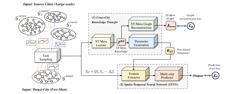
Figure 1. The framework of proposed ST-GFSL. The left side is the input of the model, in which the source cities have large-scale training samples and the target city’s is few-shot. The right side shows two main parts of ST-GFSL: (1) Cross-City Knowledge Transfer and (2) Spatio-Temporal Neural Network (STNN).

3. Preliminary

We denote the spatio-temporal graph as $\mathcal{G}_{ST}=(\mathcal{V},\mathcal{E},\mathbf{A},\mathbf{X})$. (1) $\mathcal{V}=\{v_{1},v_{2},\cdots,v_{N}\}$ denotes the nodes set, and $N=\left|\mathcal{V}\right|$ is the number of nodes. (2) $\mathcal{E}=\{e_{ij}=(v_{i},v_{j})\}\subseteq(\mathcal{V}\times\mathcal{V})$ denotes the edges set. (3) $\mathbf{A}=\{a_{ij}\}\in\mathbb{R}^{N\times N}$ is the adjacency matrix of spatio-temporal graph. $a_{ij}=1$ indicates that there is an edge between node $v_{i}$ and $v_{j}$; otherwise, $a_{ij}=0$. (4) $\mathbf{X}$ is the node feature matrix, refering to the message passing on the graph, such as traffic speed, concentration of air pollutants and passenger flow of taxis over a period of time. We take the node feature observed at time $t$ as a graph signal $\mathbf{X}^{t}\in\mathbb{R}^{N\times d}$, where $d$ is the dimension of node feature.

Problem 1.

Spatio-Temporal Graph Forecasting  Suppose we have $T$ historical spatio-temporal graph signals, and we want to predict future $M$ graph signals. The forecasting task is formulated as learning a function $f(\cdot)$ given a spatio-temporal graph $\mathcal{G}_{ST}$:

(1) $$[\mathbf{X}^{t-T+1},\cdot\cdot\cdot,\mathbf{X}^{t};\mathcal{G}_{ST}]\xrightarrow{f(\cdot)}[\mathbf{X}^{t+1},\cdot\cdot\cdot,\mathbf{X}^{t+M}]\text{.}$$

Problem 2.

Spatio-Temporal Graph Few-Shot Learning  Suppose we have a set of $P$ source spatio-temporal graphs of data-rich cities $\mathcal{G}^{source}_{1:P}=\{\mathcal{G}_{1}^{source},\cdots,\mathcal{G}_{P}^{source}\}$ and a target spatio-temporal graph of data-scarce city $\mathcal{G}^{target}$. After training on $\mathcal{G}^{source}_{1:P}$, the model is capable of leveraging the meta knowledge from multiple source graphs and is tasked to predict on a disjoint target scenario, where only few-shot structured data of $\mathcal{G}^{target}$ is available.

4. Methodology

In this section, we describe the proposed ST-GFSL framework in detail. We first give an overview of ST-GFSL, as shown in Figure 1. The left side of the figure shows the input of ST-GFSL. We transfer the knowledge from multiple cities, and the target city only has few-shot training samples. The right side of the figure is mainly composed of two parts: Spatio-Temporal Neural Network (STNN) and Cross-city Knowledge Transfer. Specifically, STNN served as the base feature extractor in ST-GFSL, where any spatial-temporal learning architecture can be used, such as Graph Neural Networks (GNNs), Recurrent Neural Networks (RNNs) and other state-of-the-art spatio-temporal graph learning models. Second, Cross-City Knowledge Transfer module transfers knowledge from multiple source cities, which are depicted in the grey dotted box of Figure 1. Concretely, we first design the ST-Meta Learner to obtain the node-level meta knowledge in both spatial and temporal domain. The non-shared feature extractor parameters $\theta_{ST}$ are generated to customize the feature extraction among source cities data and target city data. ST-Meta Graph Reconstruction is further designed for structure-aware meta training by reconstucting structure relations of different cities. The end-to-end learning process of ST-GFSL follows the MAML-based (DBLP:conf/icml/FinnAL17, ) episode learning. By mimicking few-shot scenarios in the target city, batches of few-shot training tasks are sampled to obtain a base model with strong adaptability.

4.1. Spatio-Temporal Neural Network

The Spatio-Temporal Neural Networks (STNN) can be divided into feature extractor and multi-step predictor, as shown in the bottom dotted box of Figure 1. The multi-step predictors often use one or more layers of fully connected networks  (DBLP:conf/ijcai/WuPLJZ19, ; DBLP:conf/cikm/LuGJFZ20, ; DBLP:conf/ijcai/YuYZ18, ) in literature. The feature extractor is designed according to different tasks and data characteristics, like RNN-based, CNN-based and GNN-based models. For example, in the experiment, we select the classical time series analysis networks GRU (DBLP:journals/corr/ChungGCB14, ) and TCN (DBLP:conf/cvpr/LeaFVRH17, ), as well as the superior spatio-temporal graph neural network models STGCN (DBLP:conf/ijcai/YuYZ18, ) and GWN (DBLP:conf/ijcai/WuPLJZ19, ). Since ST-GFSL is designed for a model-agnostic framework, the parameter generation method adaptively generates non-shared feature extractor parameters $\theta_{ST}$ according to corresponding model structure. Therefore, our proposed ST-GFSL enables to benefit data-scarce scenarios from recent technique breakthroughs in spatio-temporal graph learning.

4.2. ST-Meta Learner

Spatio-Temporal Meta Knowledge Learner (ST-Meta Learner) extracts the node-level meta knowledge in both spatial and temporal domains. To encode the temporal dynamics of spatio-temporal graph, we employ Gated Recurrent Unit (GRU)  (DBLP:journals/corr/ChungGCB14, ), which is widely used in time series modeling. Compared with classical RNN model, GRU retains the ability to extract long sequences and reduces the problem of gradient vanishing or exploding. Take node $v_{i}$ as an example, the node-level temporal meta knowledge $z_{i}^{tp}$ is expressed as the final state of $h_{i,t}$:

(2) $$z =\sigma\left(U^{z}x_{i,t}+W^{z}h_{i,t-1}\right)$$

$$r =\sigma\left(U^{r}x_{i,t}+W^{r}h_{i,t-1}\right)$$

$$c =\phi\left(U^{c}x_{i,t}+W^{c}\left(h_{i,t-1}\circ r\right)\right)$$

$$h_{i,t} =(1-z)\circ c+z\circ h_{i,t-1},$$

where $x_{i,t}\in\mathbb{R}^{d}$ is the input vector of node $v_{i}$ at time $t$, and $h_{i,t-1}$ is the hidden state at time $t-1$. $U^{z},U^{r},U^{c}\in\mathbb{R}^{d\times d^{\prime}}$ and $W^{z},W^{r},W^{c}\in\mathbb{R}^{d^{\prime}\times d^{\prime}}$ are weight matrices. $\circ$ is the element-wise multiplication, $\sigma$ is the nonlinear activation function sigmoid, and $\phi$ is tanh. Thus, we derive the temporal meta knowledge of one city with GRU model, denoted as $\mathbf{Z}^{tp}=(z_{1}^{tp},z_{2}^{tp},\cdots,z_{N}^{tp})\in\mathbb{R}^{N\times d^{\prime}}$.

To encode the spatial correlations of spatio-temporal graph, we utilize spatial-based graph attention network (GAT) (DBLP:conf/iclr/VelickovicCCRLB18, ) for feature extraction. Graph attention is treated as a message-passing process in which information can be passed from one node to another along edges directly. Compared with spectral-based graph neural network (DBLP:conf/nips/DefferrardBV16, ; DBLP:conf/iclr/XuSCQC19, ), GAT can adapt to various network structures. Therefore, it is suitable to learn spatial meta knowledge among multiple datasets.

Specifically, we first apply a shared linear transformation to each group of interconnected nodes and compute the attention coefficients $e_{ij}$:

(3) $$e_{ij}=attention(Wh_{i},Wh_{j}),j\in\mathcal{N}_{i}\text{,}$$

where $W\in\mathbb{R}^{d\times O}$ is the weight matrix and $\mathcal{N}_{i}$ is a set of neighbor nodes of node $v_{i}$. The attention mechanism makes $\mathbb{R}^{O}\times\mathbb{R}^{O}\rightarrow\mathbb{R}$. After that, the attention score is normalized across all choices of $j$ using the $softmax$ function:

(4) $$\alpha_{ij}=\mathop{softmax}\nolimits_{j}(e_{ij})=\frac{exp(e_{ij})}{\sum_{k\in\mathcal{N}_{i}}exp(e_{ik})}\text{.}$$

In order to obtain more abundant representation, we execute the attention mechanism for $K$ times independently and employ averaging to achieve the spatial meta knowledge of node $v_{i}$:

(5) $$z_{i}^{sp}=\sigma(\frac{1}{K}\sum\nolimits_{k=1}^{K}\sum\nolimits_{j\in\mathcal{N}_{i}}\alpha_{ij}W^{k}h_{j})\text{.}$$

Thus, we derive the spatial meta knowledge of one city $\mathbf{Z}^{sp}=(z_{1}^{sp},z_{2}^{sp},\cdots,z_{N}^{sp})\in\mathbb{R}^{N\times d^{\prime}}$.

By integrating spatio-temporal features, we obtain the meta knowledge denoted as $\mathbf{Z}^{MK}=(z_{1}^{MK},z_{2}^{MK},\cdots,z_{N}^{MK})\in\mathbb{R}^{N\times d_{MK}}$. We weighted-sum the temporal and spatial meta knowledge through a learnable ratio $\gamma$, and $\gamma\in\mathbb{R}^{d^{\prime}}$. It learns the impact from spatial or temporal domain in a data-driven manner. Compared with the classical concatenation method, it is easier to adapt the spatio-temporal characteristics of cross city data through a learnable ratio. Meanwhile, it reduces the amount of parameters for data generation, which will be further discussed in Parameter Generation. To be specific, the meta knowledge $\mathbf{Z}^{MK}$ is calculated as follows:

(6) $$\mathbf{Z}^{MK}=W^{\gamma}(\gamma\circ\mathbf{Z}^{tp}+(1-\gamma)\circ\mathbf{Z}^{sp})\text{,}$$

where $W^{\gamma}\in\mathbb{R}^{d^{\prime}\times d_{MK}}$ is the weight matrix for meta knowledge output layer, and $d_{MK}$ is the dimension of meta knowledge.

4.3. ST-Meta Graph Reconstruction

In order to express the structural information of graphs and reduces structure deviation caused by different source data distribution, ST-Meta Graph is reconstructed by meta knowledge for structure-aware learning. We predict the likelihood of an edge existing between nodes $v_{i}$ and $v_{j}$, by multiplying learned meta knowledge $z_{i}^{MK}$ and $z_{j}^{MK}$ as follows:

(7) $$p(a_{ij}|z_{i}^{MK},z_{j}^{MK})=sigmoid((z_{i}^{MK})^{T},z_{j}^{MK}).$$

As such, the ST-meta graph $\mathbf{A}_{meta}$ can be constructed as

(8) $$\mathbf{A}_{meta}=sigmoid[(\mathbf{Z^{MK}})^{T}\cdot{\mathbf{Z^{MK}}}],$$

where $(\cdot)^{T}$ is the transpose of meta knowledge matrix.

In order to guide the structure-aware learning of meta knowledge, we introduce graph reconstruction loss $\mathcal{L}_{g}$ between the ST-meta graph $A_{meta}$ and the original adjacency matrix $A$ in training process, which is calculated as follows:

(9) $$\mathcal{L}_{g}=\|\mathbf{A}_{meta}-\mathbf{A}\|^{2}.$$

4.4. Parameter Generation

After we obtain the node-level meta knowledge, due to the great difference across cities and within cities, we propose parameter generation to obtain the non-shared parameters of feature extractors for different scenarios. When the meta-knowledge of a node in target domain is similar to that of a node in multiple source domains, approximate model parameters will be obtained. In other words, the nodes in target city transfer the knowledge of source cities via parameter matching, retrieving from similar spatio-temporal characteristics.

Our parameter generation is a function $\mathcal{F}$ that takes node-level meta knowledge as input and outputs the non-shared feature extractor parameters $\theta_{ST}$. Specifically, linear layer and convolutional layer are two basic neural network units. The following introduces how to generate the parameters of these two units respectively.

Linear Layer   The expression of the linear layer is $\mathbf{Y}=\mathbf{WX}+\mathbf{b}$, where $\mathbf{W}\in\mathbb{R}^{d_{out}\times d_{in}}$ is the weight matrix and $\mathbf{b}\in\mathbb{R}^{d_{out}}$ is the bias. We can generate the model parameters $\mathbf{W}$ and $\mathbf{b}$ based on meta knowledge $\mathbf{Z}^{MK}$.

Take node $v_{i}$ as an example, based on its meta knowledge $z_{i}^{MK}\in\mathbb{R}^{d_{MK}}$, the non-shared weight matrix $\mathbf{W_{i}}$ is generated through a two-step method as shown in Figure 2. First, we perform a linear transformtion through $\mathcal{F}_{W}^{1}:\mathbb{R}^{d_{MK}}\rightarrow\mathbb{R}^{{d_{in}\cdot d_{MK}}}$ and conduct a dimension transformation: $\mathbb{R}^{{d_{in}\cdot d_{MK}}}\rightarrow\mathbb{R}^{d_{in}\times d_{MK}}$. Secondly, we perform the second linear transformation $\mathcal{F}_{W}^{2}:\mathbb{R}^{d_{in}\times d_{MK}}\rightarrow\mathbb{R}^{d_{in}\times d_{out}}$ and achieve the weight matrix $\mathbf{W_{i}}$ of node $v_{i}$. The parameter generation of bias $\mathbf{b}$ can be obtained directly by once linear transformation $\mathcal{F}_{b}$: $\mathbb{R}^{d_{MK}}\rightarrow\mathbb{R}^{d_{out}}$.

The parameter number of the weight matrix $\mathbf{W_{i}}$ generated by two-step methods is $d_{MK}\cdot[d_{in}\times d_{MK}+d_{out}]$. Compared with direct generation of one linear layer ($\mathbb{R}^{d_{MK}}\rightarrow\mathbb{R}^{d_{in}\times d_{out}}$, the parameter number is $d_{MK}\times d_{in}\times d_{out}$). Obviously, two-step generation has less parameters. For example, in our experiment, when $d_{MK}=16$, $d_{in}=8$, $d_{out}=32$, the parameter number of using the two-step method is 2560. Whereas, the parameter number of directly using the one-step method is 4096. Our parameter generation method reduces the number of parameters by 37.5%.

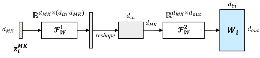
Figure 2. Parameter generation of linear weight matrix $W$.

Convolutional Layer   Similar to the linear layer, the parameter generation of the convolutional layer adopts the two-step method shown in Figure 3, where $C_{in}$ is the number of channels of input data, $C_{out}$ is the number of channels of output data, and $(K_{H},K_{W})$ is the size of the convolution kernel. Through the two-step generation, the convolutional kernel $\mathbf{W}_{i}^{conv}$ of node $v_{i}$ can be obtained after dimension reshape: $\mathbb{R}^{C_{in}\times(C_{out}\cdot K_{H}\cdot K_{W})}\rightarrow\mathbb{R}^{C_{in}\times C_{out}\times K_{H}\times K_{W}}$. For 1D-convolution, the model parameters can be obtained only by adjusting the dimension of the convolutional kernel.

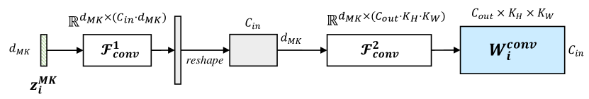
Figure 3. Parameter generation of 2D-conv weight matrix.

4.5. ST-GFSL Learning Process

To handle adaptation with few-shot scenarios, the learning process of ST-GFSL follows the MAML-based episode learning process. ST-GFSL trains the spatio-temporal graph learning model with two stage: base-model meta training and adaptation. In the base-model meta training stage, inspired by MAML (DBLP:conf/icml/FinnAL17, ), ST-GFSL imitates the adaptation process when encountering a new few-shot scene, and optimizes the adaptation capability. Different graph sequences are sampled from multiple large-scale datasets (source datasets) to form a batch of training tasks $\mathcal{T}_{ST}$. Each task $\mathcal{T}_{i}\in\mathcal{T}_{ST}$ includes $K_{\mathcal{S}}$ support sets $\mathcal{S}_{i}$ and $K_{\mathcal{Q}}$ query sets $\mathcal{Q}_{i}$. In the adaptation stage, the ST-GFSL model updates the parameters via several gradient descent steps on target domain data.

To be specific, ST-GFSL first samples batches of task sets $\mathcal{T}_{ST}$ from source datasets. Each task $\mathcal{T}_{i}\in\mathcal{T}_{ST}$ belongs to one single city, and is divided into support set $\mathcal{S}_{\mathcal{T}_{i}}$, query set $\mathcal{Q}_{\mathcal{T}_{i}}$ and $\mathcal{S}_{\mathcal{T}_{i}}\cap\mathcal{Q}_{\mathcal{T}_{i}}=\emptyset$. When learning a task $\mathcal{T}_{i}$, ST-GFSL considers a joint loss function combining prediction error loss $\mathcal{L}_{e}$ and graph reconstruction loss $\mathcal{L}_{g}$. The prediction error loss $\mathcal{L}_{e}$ is the root mean square error between multi-step prediction and ground truth of support set $\mathcal{S}_{\mathcal{T}_{i}}$:

(10) $$\mathcal{L}_{e}=\frac{1}{\|\mathcal{S}_{\mathcal{T}_{i}}\|}\sum_{(x_{j},y_{j})\in\mathcal{S}_{\mathcal{T}_{i}}}(f_{\theta}(x_{j})-y_{j})^{2}.$$

As given in Equation 9, graph reconstruction loss $\mathcal{L}_{g}$ represents the structure-aware capability of meta knowledge. Consequently, the joint loss funtion $\mathcal{L}$ is:

(11) $$\mathcal{L}=\mathcal{L}_{e}+\lambda\mathcal{L}_{g},$$

where $\lambda$ is the sum scale factor of two loss functions. To be specific, the meta objective is to minimize the sum of task loss on query sets, which is expressed as follows:

(12) $$\theta^{*}=\mathop{\arg\min}_{\theta}\sum\limits_{\mathcal{T}_{i}\in\mathcal{T}_{ST}}\mathcal{L}_{\mathcal{T}_{i}}(f_{\theta^{\prime}_{i}}).$$

In order to achieve the optimal model parameter $\theta^{*}$, Algorithm 1 outlines the base-model meta training process of ST-GFSL. First of all, we iteratively sample a batch of task sets $\mathcal{T}_{ST}$ from source datasets (line 4). With regard to training task $\mathcal{T}_{i}\in\mathcal{T}_{ST}$, task-specific model parameter $\theta_{\mathcal{T}_{i}}^{\prime}$ is updated by gradient descents for several steps (line 8-9). The gradient of $f_{\theta_{i}^{\prime}}$ based on query set $Q_{\mathcal{T}_{i}}$ is given in line 10. Finally, the general model parameters $\theta$ are trained based on the summation across all the meta-training tasks (line 11).

Input: Source spatio-temporal Graph Dataset $\mathcal{G}_{ST}$, learning rate hyperparameter $\alpha,\beta$

1

Output: Trained ST-GFSL model parameters $\theta^{*}$

2 $\theta\leftarrow$ random initalization;

3 // $\theta=\theta_{ST}+\theta_{\text{predictor}}$

4while not done do

5       Sample a batch of tasks $\mathcal{T}_{ST}\leftarrow\textsc{SampleTask}(\mathcal{G}_{ST})$ ;

6      

7      for $\mathcal{T}_{i}\in\mathcal{T}_{ST}$ do

8             $\mathcal{S}_{\mathcal{T}_{i}}\leftarrow K_{\mathcal{S}}$ support set sample from $\mathcal{T}_{i}$ ;

9            

10            $\mathcal{Q}_{\mathcal{T}_{i}}\leftarrow K_{\mathcal{Q}}$ query set sample from $\mathcal{T}_{i}$ ;

11            

12            Evaluate $\nabla_{\theta}\mathcal{L}_{\mathcal{T}_{i}}(f_{\theta})$ with $S_{\mathcal{T}_{i}}$ via Equation (11) ;

13            

14            Compute adapted parameters with gradient descent: $\theta^{\prime}_{\mathcal{T}_{i}}=\theta-\alpha\nabla_{\theta}\mathcal{L}_{\mathcal{T}_{i}}(f_{\theta})$ ;

15            

16            Evaluate $\nabla_{\theta}\mathcal{L}_{\mathcal{T}_{i}}(f(\theta^{\prime}_{\mathcal{T}_{i}}))$ with $\mathcal{Q}_{\mathcal{T}_{i}}$ via Equation (11) ;

17            

18      Update $\theta^{*}\leftarrow\theta-\beta\nabla_{\theta}\Sigma_{\mathcal{T}_{i}}\mathcal{L}_{\mathcal{T}_{i}}(f_{\theta^{\prime}_{i}})$

Algorithm 1 ST-GFSL base-model meta training

5. Experiment

In this section, we evaluate ST-GFSL in various aspects through extensive experiments. Specifically, we try to answer the following research questions through our evaluation:

• How well does ST-GFSL perform against other baseline methods on different datasets?

• How well are different spatio-temporal prediction models adaptable under the ST-GFSL framework?

• How does each proposed component of model contribute to the performance of ST-GFSL?

• How does each major hyperparameter affect the performance of ST-GFSL?

5.1. Experiment Settings

5.1.1. Dataset

In the experiment, we take traffic flow prediction as an example to verify our proposed framework. We evaluate the performance of ST-GFSL on four traffic flow datasets: METR-LA, PEMS-BAY, Didi-Chengdu, Didi-Shenzhen  (DBLP:conf/iclr/LiYS018, ; Didi_dataset, ).

In the experiment, the datasets are divided into source datasets, target dataset and test dataset. Take METR-LA as an example. When it is set as the target city, three-day data (a very small amount of data, compared with most works requiring several months of data) are selected as target data for adaptation and the rest are regarded as test data. Other three datasets (PEMS-BAY, Didi-Shenzhen and Didi-Chengdu) are used as source datasets for meta training. The same division method is used for other datasets and Z-score normalization are applied for data preprocessing.

5.1.2. Metrics

In order to fully verify the performance of our framework, we predict the traffic flow in the next 6 time steps with 12 historical time steps. Accordingly, the time step of METR-LA and PEMS-BAY datasets are 5 minutes, while Didi-Chengdu and Didi-Shenzhen datasets are 10 minutes due to the availability. Two widely used metrics are applied between the multi-step prediction and the ground truth for evaluation: Mean Absolute Error (MAE), and Root Mean Squared Error (RMSE).

Table 1. Performance comparison of few-shot learning on four traffic speed datasets. In each column, the best results are highlighted in bold and grey, and the second best is underlined.

	PEMS-BAY Dataset						METR-LA Dataset
	MAE ($\downarrow$)			RMSE ($\downarrow$)			MAE ($\downarrow$)			RMSE ($\downarrow$)
Baselines	5 min	15 min	30 min	5 min	15 min	30 min	5 min	15 min	30 min	5 min	15 min	30 min
HA	4.373	4.373	4.373	6.745	6.745	6.745	6.021	6.021	6.021	9.483	9.483	9.483
ARIMA	2.019	2.307	2.429	3.929	4.648	5.360	2.900	3.058	3.369	4.179	5.279	7.670
Target-only	1.556	1.920	2.368	3.092	4.043	5.153	2.740	3.229	3.860	4.924	6.118	7.417
Fine-tuned (Vanilla)	1.823	2.166	2.590	3.434	4.280	5.276	2.757	3.277	3.900	4.883	6.123	7.413
Fine-tuned (ST-Meta)	1.371	1.791	2.277	2.699	3.747	4.920	2.647	3.188	3.800	4.368	5.759	7.110
AdaRNN (Du2021ADARNN, )	1.248	1.928	2.749	2.084	3.796	5.725	2.513	2.897	[HTML]EFEFEF3.312	4.298	[HTML]EFEFEF5.567	[HTML]EFEFEF6.732
MAML (DBLP:conf/icml/FinnAL17, )	1.081	1.600	2.141	1.906	3.291	4.708	2.405	2.960	3.639	4.159	5.710	7.124
ST-GFSL (ours)	[HTML]EFEFEF1.073	[HTML]EFEFEF1.560	[HTML]EFEFEF2.073	[HTML]EFEFEF1.865	[HTML]EFEFEF3.180	[HTML]EFEFEF4.584	[HTML]EFEFEF2.355	[HTML]EFEFEF2.896	3.557	[HTML]EFEFEF4.099	5.588	6.961
	Didi-Chengdu Dataset						Didi-Shenzhen Dataset
	MAE ($\downarrow$)			RMSE ($\downarrow$)			MAE ($\downarrow$)			RMSE ($\downarrow$)
Baselines	10 min	30 min	60 min	10 min	30 min	60 min	10 min	30 min	60 min	10 min	30 min	60 min
HA	3.438	3.438	3.438	4.879	4.879	4.879	2.955	2.955	2.955	4.342	4.342	4.342
ARIMA	2.825	3.305	4.317	3.889	4.253	5.597	2.888	3.056	3.596	4.489	4.764	5.575
Target-only	2.386	2.700	3.085	3.516	4.017	4.569	2.071	2.454	2.834	3.154	3.793	4.422
Fine-tuned (Vanilla)	2.586	2.877	3.246	3.746	4.213	4.751	2.117	2.490	2.867	3.196	3.831	4.442
Fine-tuned (ST-Meta)	2.240	2.693	3.083	3.249	3.956	4.519	2.033	2.454	2.850	2.989	3.719	4.385
AdaRNN (Du2021ADARNN, )	2.260	2.724	3.036	3.231	3.942	[HTML]EFEFEF4.324	2.107	2.473	2.807	3.041	3.674	4.231
MAML (DBLP:conf/icml/FinnAL17, )	2.215	2.599	2.956	3.215	3.858	4.399	1.917	2.330	2.673	2.825	3.546	4.158
ST-GFSL (ours)	[HTML]EFEFEF2.188	[HTML]EFEFEF2.579	[HTML]EFEFEF2.927	[HTML]EFEFEF3.190	[HTML]EFEFEF3.820	4.339	[HTML]EFEFEF1.890	[HTML]EFEFEF2.288	[HTML]EFEFEF2.644	[HTML]EFEFEF2.763	[HTML]EFEFEF3.477	[HTML]EFEFEF4.100

5.2. Performance Comparison

5.2.1. Superiority of ST-GFSL over Baselines

First, we compare the performance of ST-GFSL with a series of baselines on four datasets:

• HA: Historical Average, which formulates the traffic flow as a seasonal process, and uses average of previous seasons as the prediction.

• ARIMA: Auto-regressive integrated moving average is a well-known model that can understand and predict future values in a time series.

• Target-only: Directly training the model on few-shot data in target domain.

• Fine-tuned (Vanilla): We first train the model on source datasets, and then fine-tune the model on few-shot data in target domain.

• Fine-tuned (ST-Meta): Compared with “Fine-tuned (Vanilla)” method, we combine the proposed parameter generation based on meta knowledge to generate non-shared parameters for the model.

• AdaRNN (Du2021ADARNN, ): A state-of-the-art transfer learning framework for non-stationary time series. This paper aims to reduce the distribution mismatch in the time series to learn an adaptive RNN-based model.

• MAML (DBLP:conf/icml/FinnAL17, ): Model-Agnostic Meta Learning (MAML), a superior meta-learning method that trains a model’s parameters such that a small number of gradient updates will lead to fast learning on a new task.

We can divide the above compared baselines into two categories: non-transfer methods and transfer methods. Non-transfer methods (HA, ARIMA, Target-only) only use the few-shot training data in target city. The rest are transfer methods, and these methods transfer the knowledge learned from multiple source datasets. Since AdaRNN uses GRU model for feature extraction, in order to maintain the fairness and consistency of comparison, other deep learning methods also use GRU model as feature extractor.

Table 1 shows the performance comparison under various methods. We make the following observations: (1) Our proposed framework ST-GFSL obtains the best results on multiple datasets in both short-term and long-term predictions, demonstating the superiority of our method. (2) In respect of AdaRNN, it performs better on some indicators, especially the mid- and long-term prediction on METR-LA dataset. The possible reason is that METR-LA is a relatively small-scale dataset with only 207 sensor nodes, and there is a strong temporal correlation between nodes. The AdaRNN’s design for temporal covariate shift makes it have a better performance in long-term prediction. However, AdaRNN is unstable when adapting to other cities (e.g. PEMS-BAY), and the experiment performance fluctuates greatly on different datasets. (3) For two fine-tuning methods, Fine-tuned (ST-Meta) based on parameter generation has a significant improvement compared to vanilla method. The results imply that our proposed non-shared parameters can better extract spatio-temporal features across the cities. (4) MAML shows good performance in the experiment. Meanwhile, MAML can be regarded as an ablation study of ST-GFSL, which will be further discussed in Section 5.3.

5.2.2. ST-GFSL for different feature extractors

ST-GFSL is a model-agnostic framework. In order to verify the versatility of the framework and further improve the prediction performance from STNN model aspect, we apply some advanced spatio-temporal data graph learning algorithms to our ST-GFSL framework. At the same time, we also train the following model directly on few-shot data in target domain to compare these two methods.

• TCN (DBLP:conf/cvpr/LeaFVRH17, ): 1D dilated convolution network-based temporal convolution network.

• STGCN (DBLP:conf/ijcai/YuYZ18, ): Spatial temporal graph convolution network, which combines graph convolution with 1D convolution.

• GWN (DBLP:conf/ijcai/WuPLJZ19, ): A convolution network structure combines graph convolution with dilated casual convolution and a self-adaptive graph.

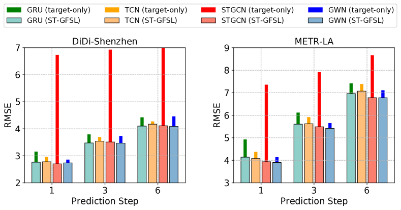
Figure 4. Performance comparison of different feature extractors on Didi-Shenzhen and METR-LA datasets.

Figure 4 shows the performance of different feature extractors on Didi-Shenzhen and METR-LA datasets. STGCN and Graph WaveNet, as the representative work of traffic speed prediction, still maintain their strong feature extraction capabilities under the ST-GFSL framework. Compared with direct training on few-shot target domain, ST-GFSL improves the performance greatly. Especially for STGCN, direct training with few-shot samples has over-fitting, which makes it impossible to predict accurately.

5.2.3. Performance across the cities

In order to explore the performance of transfering across multiple cities, we conduct experiments on different source cities, and obtain the experimental results in Figure 5. For simplicity, METR-LA dataset is denoted as “M”, PEMS-BAY dataset is denoted as “P”, Didi-Chengdu dataset is denoted as “C”, and Didi-Shenzhen dataset is denoted as “S”.

As shown in Figure 5(a), in Step #1, only use Didi-Chengdu dataset as the source city obtain the best performance. In Step #3 and Step #6, the best results are obtained by transfering the knowledge of three cities. In the short-term prediction, since Shenzhen and Chengdu are both first tier cities in China, they have more similar spatio-temporal characteristics. In long-term prediction, the knowledge transfer of multiple cities can help better predict long-term correlations. For METR-LA dataset, better performance is usually achieved when “P+S” is used as the source domain. In Step #3, the best performance can be obtained by using all datasets.

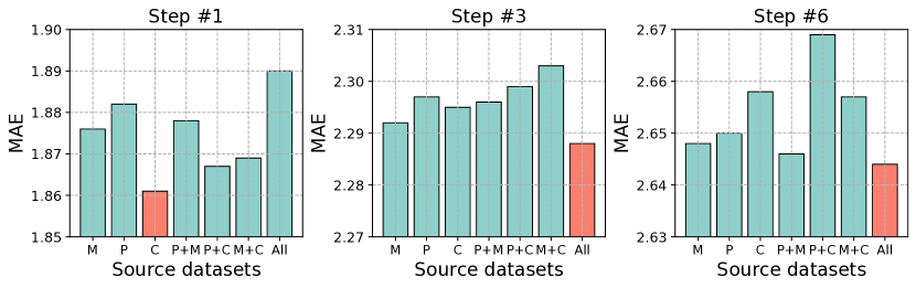
(a) Didi-Shenzhen Dataset

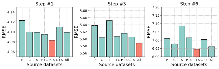
(b) METR-LA Dataset

Figure 5. Performance comparison across different source cities studied on Didi-Shenzhen and METR-LA dataset.

Table 2. Ablation Studies of ST-GFSL on Didi-Shenzhen and METR-LA dataset.

	Didi-Shenzhen Dataset						METR-LA Dataset
	MAE ($\downarrow$)			RMSE ($\downarrow$)			MAE ($\downarrow$)			RMSE ($\downarrow$)
Ablation Methods	10 min	30 min	60 min	10 min	30 min	60 min	10 min	30 min	60 min	10 min	30 min	60 min
(M1a): Use temporal meta knowledge only	1.910	2.317	2.668	2.834	3.530	4.139	[HTML]EFEFEF2.332	2.905	3.616	[HTML]EFEFEF4.077	5.619	6.991
(M1b): Use spatial meta knowledge only	1.872	2.300	2.649	2.756	3.495	4.108	2.364	2.915	3.604	4.112	5.612	6.970
(M1c): Use random initialized vectors	1.937	2.332	2.680	2.841	3.531	4.142	2.422	2.949	3.697	4.182	5.624	7.047
(M2): Remove parameter generator	1.917	2.330	2.673	2.825	3.546	4.158	2.405	2.960	3.639	4.129	5.655	7.075
(M3): Remove graph reconstruction loss $\mathcal{L}_{g}$	2.286	2.652	3.000	3.309	3.979	4.604	3.087	3.585	4.140	4.960	6.209	7.464
ST-GFSL (Ours)	[HTML]EFEFEF1.856	[HTML]EFEFEF2.290	[HTML]EFEFEF2.634	[HTML]EFEFEF2.737	[HTML]EFEFEF3.471	[HTML]EFEFEF4.052	2.387	[HTML]EFEFEF2.895	[HTML]EFEFEF3.546	4.140	[HTML]EFEFEF5.603	[HTML]EFEFEF6.963

5.3. Ablation Study

In this section, we verify the effectiveness of each module in ST-GFSL through ablation study. First of all, we only use time domain features (M1a) or only spatial domain features (M1b) as meta knowledge for parameter generation. We can see that the performance has decreased to a certain extent, which proves that the spatio-temporal joint features are more accurate for parameter generation. It is worth noting that the short-time prediction of METR-LA datasets achieves the best performance by using only temporal meta knowledge. This is because its temporal characteristics are more prominent. Furthermore, we directly use trainable random parameters to replace the learned spatio-temporal features (M1c). Since the spatio-temporal attributes are not explicitly defined, it is difficult for the random initialized vector to capture the complex and dynamic characteristics, so the performance has been greatly reduced. When we remove the parameter generator directly (M2), it degenerates into a vanilla neural network model trained by proposed ST-GFSL framework. Compared with the non-shared model parameters generated by meta knowledge, the performance has more degradation. When we subtract the graph reconstruction loss function during the training process (M3), the model has a severe performance degradation. The reason lies in that meta knowledge is not only expected to be able to extract effective spatio-temporal features, but more importantly, these features are compatible with structural information and can be generalized to more scenarios.

5.4. Case Study

In order to further explore the influence of graph reconstruction loss in cross-city knowledge transfer, we perform visual analysis on the original adjacency matrix and reconstructed ST-Meta graph. For clarity, we select the adjacency relationship of the first 30 nodes as shown in Figure 6. It can be seen that in the process of graph reconstruction, some key structural relationships (represented by red boxes in the figure) are better reconstructed. This shows that the proposed ST-meta graph reconstruction achieves expected effects, and it greatly improves the prediction performance by avoiding structural deviation as shown in the ablation study. Indeed, in the process of knowledge transfer learning across multiple cities, some structural information has not been well captured. This is a great challenge in graph data transfer learning, i.e., how to avoid structure deviation among multiple source datasets, which will become our future work.

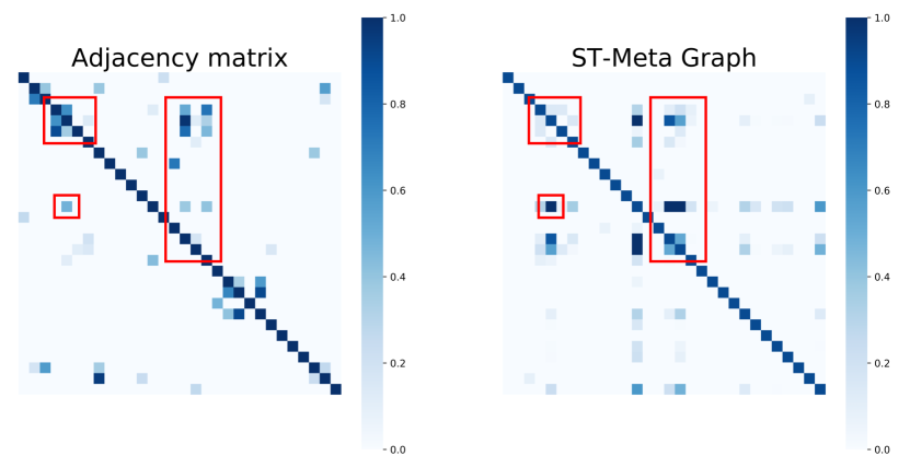
Figure 6. Case study on visualization of adjacency matrix and reconstructed ST-Meta graph.

5.5. Hyperparameter Analysis

We select the hyperparameters by analyzing the experimental results as shown in Figure 7. (1) First, we change the dimension of meta knowledge $d_{MK}$. The dimension of meta knowledge directly affects the efficiency of parameter generation. Overall, when $d_{MK}=16$, there are better performance results in both short and long term prediction. (2) Besides, the trade-off between the two loss functions is an important consideration. By observing the changes of two loss functions, we set $\lambda$ to change from 0.5 to 2.0 in the hyperparameter experiments. When we set $\lambda\textgreater 1$, we can often get better results, which also reflects the importance of graph reconstruction loss. (3) In the experiment, we all use 3-days target domain data as few-shot samples. When we adjust from 1 day to 7 days, the improvement of model performance is gradually significant in general.

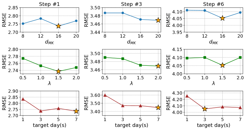
Figure 7. Hyperparameter study on Didi-Shenzhen dataset: meta knowledge dimension $d_{MK}$, sum scale factor $\lambda$ and training sample days of target city.

6. Conclusion

In this paper, we first propose a spatio-temporal graph few-shot learning framework called ST-GFSL for cross-city knowledge transfer. Non-shared feature extractor parameters based on node-level meta knowledge improve the effectiveness of spatio-temporal representation on multiple datasets and transfer the cross-city knowledge via parameter matching from similar spatio-temporal meta knowledge. ST-GFSL integrates the graph reconstruction loss to achieve structure-aware learning. Extensive experimental results in the running case of traffic speed prediction demonstrate the superiority of ST-GFSL over other baseline methods. Besides traffic speed prediction, ST-GFSL could be applied to other few-shot scenarios equipped with spatio-temporal graph learning, such as taxi demand prediction in different cities, indoor environment monitoring in different warehouses, etc. In the future, we will further explore the problem of structure deviation in knowledge transfer among graph data.

Appendix A Appendix

To support the reproducibility of the results in this paper, we have released our code and data.. Our implementation is based on torch 1.8.1, and torch-geometric 1.7.2. All the evaluated models are implemented on a server with two CPUs (Intel Xeon E5-2630 $\times$ 2) and four GPUs (NVIDIA GTX 2080 $\times$ 4). Here, we detail the datasets, evaluation metrics, baselines, and the training settings of ST-GFSL.

A.1. Datasets

We take four public dataset of traffic flow for evaluation. We adopt the same data preprocessing procedures in literature. In all those datasets, we apply Z-Score normalization for data preprocessing. The missing values are filled by the linear interpolation. To construct the road network graph, each traffic sensor or road segment is considered as a vertex and we compute the pairwise road network distances between sensors. The adjacency matrix of the nodes is constructed by road network distance with a thresholded Gaussian kernel. The detailed information of each dataset is shown in Table 3.

Table 3. Statistics of the traffic datasets in experiment.

Datasets	METR-LA	PEMS-BAY	Didi-Chengdu	Didi-Shenzhen
# Nodes	207	325	524	627
# Edges	1,722	2,694	1,120	4,845
Interval	5 min	5 min	10 min	10 min
Time span	34,272	52,116	17,280	17,280
Mean	58.274	61.776	29.023	31.001
Std	13.128	9.285	9.662	10.969

• METR-LA [27]: Traffic data are collected from observation sensors in the highway of Los Angeles County. We use 207 sensors and 4 months of data dated from 1st Mar 2012 until 30th Jun 2012 in the experiment. The readings of the sensors are aggregated into 5-minutes windows.

• PEMS-BAY [27]: PEMS-BAY dataset contains 6 months of data recorded by 325 traffic sensors ranging from January 1st, 2017 to June 30th, 2017 in the Bay Area.

• Didi-Chengdu [28]: Traffic index dataset of Chengdu, China, provided by Didi Chuxing GAIA Initiative. We select data from January to April 2018, with 524 roads in the core urban area of Chengdu. The data collection interval is 10 minutes.

• Didi-Shenzhen [28]: Traffic index dataset of Shenzhen, China, provided by Didi Chuxing GAIA Initiative. We select data from January to April 2018, and it contains 627 roads in downtown Shenzhen. The data collection interval is 10 minutes.

A.2. Evaluation Metrics

To verify the effectiveness of the proposed algorithm, we evaluate the results of multi-step prediction. Two widely used metrics are applied between the multi-step prediction $\hat{y}$ and the ground truth $y$ for evaluation: Mean Absolute Error (MAE), and Root Mean Squared Error (RMSE).

• Mean Absolute Error (MAE)

  $$MAE(y,\hat{y})=\frac{1}{N}\sum\nolimits_{i=1}^{N}\left|\hat{y_{i}}-y_{i}\right|\text{.}$$

• Root Mean Squared Error (RMSE)

  $$RMSE(y,\hat{y})=\sqrt{\frac{1}{N}\sum\nolimits_{i=1}^{N}(\hat{y_{i}}-y_{i})^{2}}\text{.}$$

A.3. Baselines

The details of the baselines are as follows:

• HA: Historical Average, which formulates the traffic flow as a seasonal process, and uses average of previous seasons as the prediction. We use the few-shot sample of target city to calculate the average traffic speed of each node in one day, and use this as the baseline to predict the future values.

• ARIMA: Auto-regressive integrated moving average is a well-known model that can understand and predict future values in a time series. The model are implemented using the statsmodel python package. The orders are (3,0,1).

• Target-only: We directly use the few-shot training samples of target domain to train the model, without utilizing the training data of other source cities for knowledge transfer.

• Fine-tuned (Vanilla): We first train the model on source datasets, and then fine-tune the model on few-shot data in target domain. Here we used all the multiple source cities for training.

• Fine-tuned (ST-Meta): Compared with “Fine-tuned (Vanilla)” method, we combine the proposed parameter generation based on meta knowledge to generate non-shared parameters for the model.

• AdaRNN [29]: A state-of-the-art transfer learning framework for non-stationary time series. This paper aims to reduce the distribution mismatch in the time series to learn an adaptive RNN-based model. In the experiment, we predict each node independently, and the traffic speed of a single node can be analyzed as a typical time series as the setting in AdaRNN.

• MAML [14]: Model-Agnostic Meta Learning (MAML), a superior meta-learning method that trains a model’s parameters such that a small number of gradient updates will lead to fast learning on a new task. It learns a better initialization model from multiple tasks to supervise the target task.

A.4. Training settings

In the experiment, we use $T=12$ historical time steps to predict the traffic speed of the next $M=6$ time steps. Due to different time resolutions, Didi-Shenzhen and Didi-Chengdu datasets will predict the results in the next 60 minutes, while METR-LA and PEMS-BAY datasets will predict the next 30 minutes’. The ST-GFSL framework is trained by Adam optimizer with learning rate decay in both inner loop and outer loop. In ST-Meta Learner, the number of GAT is set to 2, and the the GRU layer is set to 1. Totally, there are several important hyperparameters in our model, and we set them as: the dimension of meta knowledge $d_{MK}=16$, task learning rate $\alpha=0.01$, meta-training rate $\beta=0.001$, task batch number $\|\mathcal{T}\|=5$, and sum scale factor of two loss function $\lambda=1.5$.

In order to compare the performance of different feature extractors in the ST-GFSL framework, we also used three advanced models in this paper, which are described in detail as follows:

• TCN [23]: 1D dilated convolution network-based temporal convolution network. We used the addition of two TCN models as the feature extractor. The size of the dilated convolution kernel is set to 2 and 3 respectively.

• STGCN [21]: Spatial temporal graph convolution network, which combines graph convolution with 1D causal convolution. The layer of STGCN block is set to 2, and use one-layer FC as the multi-step predictor.

• GWN [1]: A convolution network structure combines graph convolution with dilated casual convolution, which introduces a self-adaptive graph to capture the hidden spatial dependency. The block of GWN is set to 4, and the layer of GWN blocks is set to 2.

References

- [1] Zonghan Wu, Shirui Pan, Guodong Long, Jing Jiang, and Chengqi Zhang. Graph wavenet for deep spatial-temporal graph modeling. In Proceedings of the Twenty-Eighth International Joint Conference on Artificial Intelligence, IJCAI 2019, Macao, China, August 10-16, 2019, pages 1907–1913, 2019.
- [2] Bin Lu, Xiaoying Gan, Haiming Jin, Luoyi Fu, and Haisong Zhang. Spatiotemporal adaptive gated graph convolution network for urban traffic flow forecasting. In The 29th ACM International Conference on Information and Knowledge Management, Virtual Event, Ireland, October 19-23, 2020, pages 1025–1034. ACM, 2020.
- [3] Junchen Ye, Leilei Sun, Bowen Du, Yanjie Fu, and Hui Xiong. Coupled layer-wise graph convolution for transportation demand prediction. In Thirty-Fifth AAAI Conference on Artificial Intelligence, AAAI 2021, Virtual Event, February 2-9, 2021, pages 4617–4625, 2021.
- [4] Zhenlong Zhu, Ruixuan Li, Minghui Shan, Yuhua Li, Lu Gao, Fei Wang, Jixing Xu, and Xiwu Gu. Tdp: Personalized taxi demand prediction based on heterogeneous graph embedding. In Proceedings of the 42nd International ACM SIGIR Conference on Research and Development in Information Retrieval, SIGIR’19, page 1177–1180, New York, NY, USA, 2019.
- [5] Chunyang Wang, Yanmin Zhu, Tianzi Zang, Haobing Liu, and Jiadi Yu. Modeling inter-station relationships with attentive temporal graph convolutional network for air quality prediction. In WSDM ’21, The Fourteenth ACM International Conference on Web Search and Data Mining, Virtual Event, Israel, March 8-12, 2021, pages 616–634. ACM, 2021.
- [6] Leye Wang, Xu Geng, Xiaojuan Ma, Feng Liu, and Qiang Yang. Cross-city transfer learning for deep spatio-temporal prediction. In Proceedings of the Twenty-Eighth International Joint Conference on Artificial Intelligence, IJCAI 2019, Macao, China, August 10-16, 2019, pages 1893–1899, 2019.
- [7] Ying Wei, Yu Zheng, and Qiang Yang. Transfer knowledge between cities. In Proceedings of the 22nd ACM SIGKDD International Conference on Knowledge Discovery and Data Mining, KDD ’16, page 1905–1914, New York, NY, USA, 2016.
- [8] Huaxiu Yao, Yiding Liu, Ying Wei, Xianfeng Tang, and Zhenhui Li. Learning from multiple cities: A meta-learning approach for spatial-temporal prediction. In The World Wide Web Conference, WWW ’19, page 2181–2191, New York, NY, USA, 2019.
- [9] Luis Moreira-Matias, Joao Gama, Michel Ferreira, Joao Mendes-Moreira, and Luis Damas. Predicting taxi–passenger demand using streaming data. IEEE Transactions on Intelligent Transportation Systems, 14(3):1393–1402, 2013.
- [10] Lei Bai, Lina Yao, Salil S. Kanhere, Xianzhi Wang, and Quan Z. Sheng. Stg2seq: Spatial-temporal graph to sequence model for multi-step passenger demand forecasting. In Proceedings of the Twenty-Eighth International Joint Conference on Artificial Intelligence, IJCAI 2019, Macao, China, August 10-16, 2019, pages 1981–1987, 2019.
- [11] Tien Huu Do, Evaggelia Tsiligianni, Xuening Qin, Jelle Hofman, Valerio Panzica La Manna, Wilfried Philips, and Nikos Deligiannis. Graph-deep-learning-based inference of fine-grained air quality from mobile iot sensors. IEEE Internet of Things Journal, 7(9):8943–8955, 2020.
- [12] Zheyi Pan, Yuxuan Liang, Weifeng Wang, Yong Yu, Yu Zheng, and Junbo Zhang. Urban traffic prediction from spatio-temporal data using deep meta learning. In Proceedings of the 25th ACM SIGKDD International Conference on Knowledge Discovery & Data Mining, KDD 2019, Anchorage, AK, USA, August 4-8, 2019, pages 1720–1730. ACM, 2019.
- [13] Zheyi Pan, Wentao Zhang, Yuxuan Liang, Weinan Zhang, Yong Yu, Junbo Zhang, and Yu Zheng. Spatio-temporal meta learning for urban traffic prediction. IEEE Transactions on Knowledge and Data Engineering, pages 1–1, 2020.
- [14] Chelsea Finn, Pieter Abbeel, and Sergey Levine. Model-agnostic meta-learning for fast adaptation of deep networks. In Proceedings of the 34th International Conference on Machine Learning, ICML 2017, Sydney, NSW, Australia, 6-11 August 2017, volume 70 of Proceedings of Machine Learning Research, pages 1126–1135. PMLR, 2017.
- [15] Jake Snell, Kevin Swersky, and Richard S. Zemel. Prototypical networks for few-shot learning. In Annual Conference on Neural Information Processing Systems 2017, December 4-9, 2017, Long Beach, CA, USA, pages 4077–4087, 2017.
- [16] Qianru Sun, Yaoyao Liu, Tat-Seng Chua, and Bernt Schiele. Meta-transfer learning for few-shot learning. In IEEE Conference on Computer Vision and Pattern Recognition, CVPR 2019, Long Beach, CA, USA, June 16-20, 2019, pages 403–412. Computer Vision Foundation / IEEE, 2019.
- [17] Fan Zhou, Chengtai Cao, Kunpeng Zhang, Goce Trajcevski, Ting Zhong, and Ji Geng. Meta-gnn: On few-shot node classification in graph meta-learning. In Proceedings of the 28th ACM International Conference on Information and Knowledge Management, CIKM 2019, Beijing, China, November 3-7, 2019, pages 2357–2360, 2019.
- [18] Zemin Liu, Yuan Fang, Chenghao Liu, and Steven CH Hoi. Relative and absolute location embedding for few-shot node classification on graph. In Proceedings of the AAAI Conference on Artificial Intelligence, volume 35, pages 4267–4275, 2021.
- [19] Huaxiu Yao, Chuxu Zhang, Ying Wei, Meng Jiang, Suhang Wang, Junzhou Huang, Nitesh V. Chawla, and Zhenhui Li. Graph few-shot learning via knowledge transfer. In The Thirty-Fourth AAAI Conference on Artificial Intelligence, AAAI 2020, New York, NY, USA, February 7-12, 2020, pages 6656–6663, 2020.
- [20] Kaize Ding, Jianling Wang, Jundong Li, Kai Shu, Chenghao Liu, and Huan Liu. Graph prototypical networks for few-shot learning on attributed networks. In The 29th ACM International Conference on Information and Knowledge Management, Virtual Event, Ireland, October 19-23, 2020, pages 295–304. ACM, 2020.
- [21] Bing Yu, Haoteng Yin, and Zhanxing Zhu. Spatio-temporal graph convolutional networks: A deep learning framework for traffic forecasting. In Proceedings of the Twenty-Seventh International Joint Conference on Artificial Intelligence, IJCAI 2018, July 13-19, 2018, Stockholm, Sweden, pages 3634–3640, 2018.
- [22] Junyoung Chung, Çaglar Gülçehre, KyungHyun Cho, and Yoshua Bengio. Empirical evaluation of gated recurrent neural networks on sequence modeling, 2014.
- [23] Colin Lea, Michael D. Flynn, René Vidal, Austin Reiter, and Gregory D. Hager. Temporal convolutional networks for action segmentation and detection. In 2017 IEEE Conference on Computer Vision and Pattern Recognition, CVPR 2017, Honolulu, HI, USA, July 21-26, 2017, pages 1003–1012, 2017.
- [24] Petar Velickovic, Guillem Cucurull, Arantxa Casanova, Adriana Romero, Pietro Liò, and Yoshua Bengio. Graph attention networks. In 6th International Conference on Learning Representations, ICLR 2018, Vancouver, BC, Canada, April 30 - May 3, 2018, Conference Track Proceedings, 2018.
- [25] Michaël Defferrard, Xavier Bresson, and Pierre Vandergheynst. Convolutional neural networks on graphs with fast localized spectral filtering. In Annual Conference on Neural Information Processing Systems 2016, December 5-10, 2016, Barcelona, Spain, pages 3837–3845, 2016.
- [26] Bingbing Xu, Huawei Shen, Qi Cao, Yunqi Qiu, and Xueqi Cheng. Graph wavelet neural network. In 7th International Conference on Learning Representations, ICLR 2019, New Orleans, LA, USA, May 6-9, 2019, 2019.
- [27] Yaguang Li, Rose Yu, Cyrus Shahabi, and Yan Liu. Diffusion convolutional recurrent neural network: Data-driven traffic forecasting. In 6th International Conference on Learning Representations, ICLR 2018, Vancouver, BC, Canada, April 30 - May 3, 2018, Conference Track Proceedings, 2018.
- [28] Didi-Chuxing. Didi chuxing gaia initiative. https://gaia.didichuxing.com, 2020. Accessed: 2020-02-14.
- [29] Yuntao Du, Jindong Wang, Wenjie Feng, Sinno Pan, Tao Qin, Renjun Xu, and Chongjun Wang. Adarnn: Adaptive learning and forecasting for time series. In Proceedings of the 30th ACM International Conference on Information & Knowledge Management (CIKM), 2021.