CREAM: Weakly Supervised Object Localization via
Class RE-Activation Mapping
Abstract
Weakly Supervised Object Localization (WSOL) aims to localize objects with image-level supervision. Existing works mainly rely on Class Activation Mapping (CAM) derived from a classification model. However, CAM-based methods usually focus on the most discriminative parts of an object (i.e., incomplete localization problem). In this paper, we empirically prove that this problem is associated with the mixup of the activation values between less discriminative foreground regions and the background. To address it, we propose Class RE-Activation Mapping (CREAM), a novel clustering-based approach to boost the activation values of the integral object regions. To this end, we introduce class-specific foreground and background context embeddings as cluster centroids. A CAM-guided momentum preservation strategy is developed to learn the context embeddings during training. At the inference stage, the re-activation mapping is formulated as a parameter estimation problem under Gaussian Mixture Model, which can be solved by deriving an unsupervised Expectation-Maximization based soft-clustering algorithm. By simply integrating CREAM into various WSOL approaches, our method significantly improves their performance. CREAM achieves the state-of-the-art performance on CUB, ILSVRC and OpenImages benchmark datasets. Code will be available at https://github.com/Jazzcharles/CREAM.
1 Introduction
Weakly Supervised Object Localization (WSOL) aims to localize objects only belonging to one class in each image using image-level supervision [38, 34, 6, 33]. WSOL alleviates massive efforts in obtaining fine annotations.
Prior works mainly follow the pipeline of training a classification network then deriving the Class Activation Mapping (CAM) [38] for WSOL. The foreground region is determined by the CAM values larger than the threshold. However, CAM only highlights the most discriminative regions (i.e., incomplete localization). Existing works seek to discover the complete object via adversarial erasing [22, 34], spatial regularization [15, 19] or attention mechanism [6]. Most of them still acquire the activation maps via a classification pipeline like CAM to answer “which pixels contribute to the class prediction”.
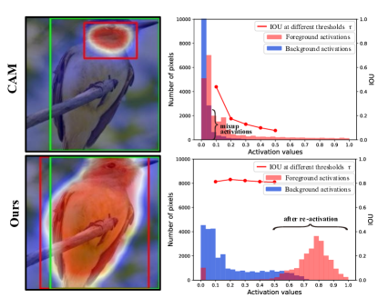
In this paper, we argue that the incomplete localization problem of CAM is associated with the mixup of the activation values between less discriminative foreground regions and the background. Figure 1 (top) illustrates the distributions of foreground activations (red) and background activations (blue) in CAM. High activations are only dominated by the most discriminative parts (e.g., bird head). In contrast, numerous low activations belong to both the less discriminative parts (e.g., bird body) and the background, making them hard to distinguish. The mixup activations bring the challenge of balancing the precision and the recall of the foreground region. Specifically, the widely adopted threshold =0.2 [38, 22, 6] appears too large to completely cover foreground object. Whereas tuning a very small threshold (e.g., <0.1) may induce significant false-positive localizations. Moreover, due to mixup activations, a slight change to the threshold leads to a drastic change to the IOU when is small (red curve), and therefore the localization result is sensitive to the threshold. Choe et al. [5] also revealed that a well chosen threshold could lead to a misconception of improvement over CAM. This indicates the infeasibility of improving CAM by simply controlling the threshold.
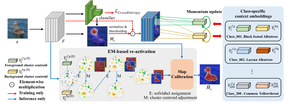
To address the above challenges, we propose Class RE-Activation Mapping (CREAM), a novel framework for WSOL. We rethink the WSOL task by answering “whether the pixel is more similar to the foreground or the background”. In particular, we introduce class-specific foreground (background) context embeddings describing the common foreground (background) features. During training, a momentum preservation strategy is developed to update the context embeddings under the guidance of CAM. With abundant context information, the learned embeddings serve as initial foreground (background) cluster centroids for each class. During inference, we cast the re-activation mapping as a parameter estimation problem formulated under the Gaussian Mixture Model (GMM) framework. We solve it by deriving an Expectation-Maximization (EM) based soft-clustering algorithm. CREAM boosts the activation values of the integral object, eases the foreground-background separation and shows robustness to the threshold, as shown in Figure 1 (bottom). It outperforms prior WSOL works on CUB, ILSVRC and OpenImages datasets.
To sum up, the contributions of this paper are as follows:
-
•
We propose CREAM, a clustering-based method, to solve the mixup of activations between less discriminative foreground regions and the background by boosting the activations of the integral object regions.
-
•
We devise a CAM-guided momentum preservation strategy to learn the class-specific context embeddings and use them as initial cluster centroids for re-activation mapping.
-
•
We regard re-activation mapping as a parameter estimation problem under the GMM framework and solve it by deriving an EM-based soft-clustering algorithm.
-
•
CREAM achieves state-of-the-art localization performance on CUB, ILSVRC and OpenImages benchmark datasets. It can also serve as a plug-and-play method in a variety of existing WSOL approaches.
2 Related Work
2.1 Weakly supervised object localization
Regressor-free WSOL methods. Following Class Activation Mapping (CAM) [38], most approaches obtain the class prediction and the localization map with a classification network only [22, 27, 35, 37, 6, 2]. To tackle the incomplete localization problem of CAM, several methods adopted an iterative erasing strategy on input images [22, 32] or feature maps [27, 35] to force the network’s attention to the remaining parts of an object. Inspired by the attention mechanism, Zhang et al. [36] leveraged pixel-level similarities across different objects to acquire their consistent feature representations. RCAM [1] offered thresholded average pooling, negative weight clamping and percentile thresholding as ways to improving CAM. SEM [37] sampled top-K activations as foreground seeds and used them to assign the label for each pixel. Xie et al.[28] generated compact activation maps under the guidance of low-level features. Different from these approaches, our method obtains the activation map via an EM-based soft clustering mechanism, which naturally relieves the incomplete localization problem.
Regressor-based WSOL methods. This category of work [33, 15, 25, 10] disentangles the WSOL task into image classification and class-agnostic object localization. The intuition is that a model’s high localization performance is accompanied by low classification accuracy in early epochs, and vice versa in late epochs. The disentanglement aims to boost both the localization and classification performance. PSOL [33] first proved that training an additional regression network for bounding box prediction yielded great improvement. The bounding box annotations were obtained using an unsupervised co-localization approach [26]. Lu et al. [15] applied a classifier, a generator and a regressor to impose the geometry constraint for compact object discovery. SLT-Net [10] produced robust localization results with semantic and visual stimuli tolerance strengthening mechanisms. With the assistance of a separate regression network, these works achieve superior localization performance over most regressor-free methods. Our CREAM is applicable to both the regressor-free and regressor-based methods.
2.2 EM-based deep learning methods
Expectation-Maximization (EM) algorithm has been frequently adopted in deep learning in recent works [12, 31, 14, 16, 3, 30]. Hinton et al. [12] introduced EM routing to group capsules for part-whole relationship construction. Yang et al. [31] designed prototype mixture models for few-shot segmentation. They applied EM algorithm to estimate the models’ mean vectors for query images. Biggs et al. [3] used EM algorithm to learn a 3D shape prior for animal reconstruction. Most prior works jointly optimized the parameters in the EM algorithm and the network’s parameters during training. In comparison, we derive an EM based algorithm during inference as an unsupervised soft-clustering mechanism for foreground-background separation.
3 Methodology
3.1 Revisiting class activation mapping for WSOL
Let be the feature map in the last convolutional layer, and each corresponds to the feature map at channel . is the weight for the channel with regard to class . The class activation mapping is defined as:
| (1) |
Meanwhile, the class prediction can be re-written as:
| (2) |
where and stand for the spatial location. In this way, solving WSOL with CAM can be interpreted as answering “which pixels contribute to the class prediction”.
To produce the final bounding box/mask for WSOL evaluation, is then normalized to [0, 1] and thresholded by a pre-defined hyperparameter . Only the CAM values greater than are considered as foreground pixels. However, the activation values of the less discriminative foreground region and the background are indistinguishable, as shown in Figure 1 (top). CAM is thus prone to the incomplete localization problem.
3.2 Class re-activation mapping
For each image, our goal is to discover its foreground region by mapping each pixel into foreground or background cluster. We start by introducing and as the context embeddings. and represent the common foreground and background context features in class , respectively. They can also be regarded as two cluster centroids for each class. The ways to learning the embeddings and realizing re-activation based on the learned embeddings are described below. Figure 2 shows the framework of our proposed Class RE-Activation Mapping.
Training stage: context embedding learning. We follow exactly the same training procedure and the cross-entropy loss as CAM [38] except that we maintain the context embeddings additionally. The basic idea of context embedding learning is to use the foreground (background) features of current mini-batch images to update the embeddings. First, we perform hard-thresholding on CAM to obtain the one-hot binary masks , as foreground-background indicators, which are calculated as:
| (3) |
where is an indicator function; and is set to as suggested in [38]. The foreground (background) features can be retrieved by the element-wise multiplication of the original feature and the mask . For each sample , we exploit a momentum preservation strategy on the foreground (background) embeddings using the spatial average of the foreground (background) features. Suppose , the update of the embeddings with regard to class is given by:
| (4) |
where is the value at location ; is the momentum coefficient; counts the number of non-zero elements. With rich context features, the trained and act as the initial cluster centroids for re-activation.
Inference stage: re-activation mapping. At the inference stage, we formulate re-activation mapping as a parameter estimation problem under Gaussian Mixture Model (GMM) [20] and solve it using an unsupervised Expectation-Maximization (EM) algorithm [7]. EM algorithm is a generalization of Maximum Likelihood Estimation for probabilistic models with latent variables [4].
Problem Formulation. For each sample , the log-likelihood we aim to maximize is given by:
| (5) |
where is the model parameter. In particular, we define the model for each pixel as a probability mixture model of two distributions, i.e., foreground distribution and background distribution:
| (6) |
where the mixing weights and +=1. The foreground (background) base model is designed to measure the similarity between the image features and the learned embeddings. Instead of using the RBF kernel in GMM, the choice of base models is Gaussian function based on cosine similarity for implementation efficiency:
| (7) |
where is a scale parameter. Next, we describe the application of EM in solving the mixture model. We define as the latent variables. represents the probability of belonging to foreground at location .
E-step. In the E-step, current parameters are utilized to evaluate the posterior distribution of the latent variables, i.e., and . In each iteration , assuming the model parameters are fixed, the latent variables are computed as:
| (8) |
From the perspective of soft clustering, Eq. (8) calculates the similarity between each pixel feature and context embeddings (i.e., centroids), and assigns a soft label () to each pixel. Different from the random initialization in EM, in our case, the initial embeddings have gained sufficient class-specific features from context embedding learning.
M-step. In the M-step, the purpose is to adjust the context embeddings by maximizing the expected log-likelihood of the image features using the computed latent variables. This enables class-specific context embeddings to be image-specific. The new model parameters can be obtained by:
| (9) |
where . and are updated by the weighted mean of the features and the effective number of pixels assigned to the foreground, respectively.
Eqs. (8) and (9) execute alternately until convergence. and successfully mark the entire object regions. CREAM naturally re-activates the values of the integral object regions by assigning a higher probability of being foreground to them. The consequent benefit of gaining the activation map via feature clustering is that it avoids Global Average Pooling layer’s bias towards small areas [1].
3.3 Map calibration
So far, and have been serving as object localization results. According to the underlying assumption of CAM, foreground objects correspond to high values in the activation map. However, we cannot tell from Eqs. (7) and (8) whether higher or lower values correspond to the foreground regions in . To be specific, is expected to be the final localization map only if its foreground regions have higher values. Otherwise, should be chosen. To deal with this uncertainty, we perform map calibration by leveraging their averaged probabilities of being the foreground, i.e., and as:
| (10) |
where the foreground region can be similarly retrieved under the guidance of CAM as to the training stage. The calibrated foreground map is defined as the one with greater averaged probability:
| (11) |
To further reduce the re-activations over background regions, the final re-activation map is formulated as the sum of the calibrated foreground map and CAM:
| (12) |
| Methods | CUB (MaxBoxAccV2) | ILSVRC (MaxBoxAccV2) | OpenImages (PxAP) | Total | |||||||||
|---|---|---|---|---|---|---|---|---|---|---|---|---|---|
| VGG | Inception | ResNet | Mean | VGG | Inception | ResNet | Mean | VGG | Inception | ResNet | Mean | Mean | |
| Center baseline | 54.4 | 54.4 | 54.4 | 54.4 | 48.9 | 48.9 | 48.9 | 48.9 | 45.8 | 45.8 | 45.8 | 45.8 | 52.3 |
| CAM[38] | 63.7 | 56.7 | 63.0 | 61.1 | 60.0 | 63.4 | 63.7 | 62.4 | 58.3 | 63.2 | 58.5 | 60.0 | 61.2 |
| HaS[22] | +0.0 | -3.3 | +1.7 | -0.5 | +0.6 | +0.3 | -0.3 | +0.2 | -0.2 | -5.1 | -2.6 | -2.6 | -1.0 |
| ACoL[34] | -6.3 | -0.5 | +3.5 | -1.1 | -2.6 | +0.3 | -1.4 | -1.2 | -4.0 | -6.0 | -1.2 | -3.7 | -2.0 |
| SPG[35] | -7.4 | -0.8 | -2.6 | -3.6 | -0.1 | -0.1 | -0.4 | -0.2 | +0.0 | -0.9 | -1.8 | -0.9 | -1.6 |
| ADL[6] | +2.6 | +2.1 | -4.6 | +0.0 | -0.2 | -2.0 | +0.0 | -0.7 | +0.4 | -6.4 | -3.3 | -3.1 | -1.3 |
| CutMix[32] | -1.4 | +0.8 | -0.2 | -0.3 | -0.6 | +0.5 | -0.4 | -0.2 | -0.2 | -0.7 | -0.8 | -0.6 | -0.3 |
| RCAM[1] | - | - | - | - | - | - | - | - | +1.3 | +0.1 | +2.4 | +1.3 | - |
| CAM_IVR[13] | +1.5 | +4.1 | +3.9 | +3.1 | +1.5 | +2.1 | +1.9 | +1.8 | +1.0 | +0.4 | +0.5 | +0.6 | +1.8 |
| +7.8 | +7.5 | +10.5 | +8.6 | +6.2 | +5.5 | +3.7 | +5.1 | +3.7 | +1.4 | +6.2 | +3.8 | +5.8 | |
4 Experiments
4.1 Experimental setup
Datasets. We evaluate our method on three popular WSOL benchmark datasets, i.e., Caltech-UCSD-Birds-200-2011 (CUB) [24], ILSVRC [8] and OpenImages [5]. CUB is a fine-grained bird dataset with 200 species. The training set and testing set contains 5,994 and 5,794 images, respectively. ILSVRC contains 1.2 million training images and 50,000 validation images of 1,000 classes. Both CUB and ILSVRC datasets provide bounding boxes for WSOL evaluation. OpenImages is a recently proposed benchmark. It consists of 29,819, 2,500 and 5,000 images of 100 categories for training, validation and testing, respectively.
Evaluation metrics. Following [34, 33], we use three threshold-dependent evaluation metrics: Top-1 localization accuracy (Top-1 Loc), Top-5 localization accuracy (Top-5 Loc) and GT-Known localization accuracy (GT-Known). We adopt two recently proposed metrics, MaxBoxAccV2 and Pixel-wise Average Precision (PxAP) [5]. They directly measure the localization performance regardless of the class prediction and the choice of threshold .
Implementation details. We implement our method on three backbones pre-trained on ImageNet [8], i.e., VGG16 [21], InceptionV3 [23] and ResNet50 [11]. Following [34, 35, 5], the input images are resized to 256256 and randomly cropped to 224224. We perform random horizontal flip during training. We train 50/6/10 epochs on CUB, ILSVRC and OpenImages, respectively. The initial learning rate is 0.001 and divided by 10 for every 15/2/3 epochs on three datasets, respectively. Notably, we set scale of the learning rate to the classifier due to its random initialization. The min-max normalization strategy is adopted in all the experiments. The SGD optimizer is used with the batch size of 32. On average, the total iterations =2 is sufficient to cover foreground objects. By default, =8 and =0.8 are set across all datasets. Specifically, we introduce two variants of CREAM in the experiments:
-
•
stands for the base CREAM model that only uses the classification network (i.e., regressor-free) to obtain both the class prediction and the localization result, as shown in Figure 2. Most ablation studies are conducted over .
-
•
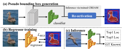
includes a regressor to predict the final bounding box following recent regressor-based methods [33, 10], as illustrated in Figure 3. First, we apply the trained model to generate the pseudo bounding boxes for the training set. We then train a regressor from scratch using the pseudo bounding boxes as the ground truth. The MSE loss is calculated over four coordinates of the box. During inference, the class prediction and object location are derived from the classifier and the regressor, respectively. By disentangling the WSOL task into classification and class-agnostic object localization, solves the contradiction that the localization accuracy gradually decreases while the classification accuracy increases during training [17, 33].
| Methods | Backbone | Localization Accuracy | ||
|---|---|---|---|---|
| Top-1 Loc. | Top-5 Loc. | GT-Known | ||
| CAM [38] | VGG16 | 44.15 | 52.16 | 56.00 |
| CutMix [32] | VGG16 | 43.45 | - | - |
| ACoL [34] | VGG16 | 45.92 | 56.51 | 54.10 |
| SPG [35] | VGG16 | 48.93 | 57.85 | 58.90 |
| HaS-32 [22] | VGG16 | 49.50 | - | 71.60 |
| ADL [6] | VGG16 | 52.36 | - | 75.40 |
| DANet [29] | VGG16 | 52.52 | 61.96 | 67.70 |
| MEIL [17] | VGG16 | 57.46 | - | 73.80 |
| SPA [19] | VGG16 | 60.27 | 72.50 | 77.29 |
| RCAM [1] | VGG16 | 61.30 | - | 80.72 |
| GC-Net [15] | VGG16 | 63.24 | 75.54 | 81.10 |
| PSOL [33] | VGG16 | 66.30 | 84.05 | - |
| SLT-Net [10] | VGG16 | 67.80 | - | 87.60 |
| ORNet [28] | VGG16 | 67.74 | 80.77 | 86.20 |
| FAM [18] | VGG16 | 69.26 | - | 89.26 |
| VGG16 | 70.44 | 85.67 | 90.98 | |
| DANet [29] | InceptionV3 | 49.45 | 60.46 | 67.00 |
| ADL [6] | InceptionV3 | 53.04 | - | - |
| SPA [19] | InceptionV3 | 53.59 | 66.50 | 72.14 |
| I2C [36] | InceptionV3 | 55.99 | 68.34 | 72.60 |
| PSOL [33] | InceptionV3 | 65.51 | 83.44 | - |
| SLT-Net [10] | InceptionV3 | 66.10 | - | 86.50 |
| FAM [18] | InceptionV3 | 70.67 | - | 87.25 |
| TS-CAM [9] | Deit-S | 71.30 | 83.80 | 87.70 |
| InceptionV3 | 71.76 | 86.37 | 90.43 | |
| Methods | Backbone | Localization Accuracy | ||
|---|---|---|---|---|
| Top-1 Loc. | Top-5 Loc. | GT-Known | ||
| CAM[38] | VGG16 | 42.80 | 54.86 | 59.00 |
| CutMix[32] | VGG16 | 43.45 | - | - |
| RCAM[1] | VGG16 | 44.69 | - | 61.69 |
| ADL[6] | VGG16 | 45.92 | - | - |
| ACoL[34] | VGG16 | 45.83 | 59.43 | 62.96 |
| MEIL[17] | VGG16 | 46.81 | - | - |
| I2C[36] | VGG16 | 47.41 | 58.51 | 63.90 |
| SEM[37] | VGG16 | 47.53 | - | 63.74 |
| SPA[19] | VGG16 | 49.56 | 61.32 | 65.05 |
| PSOL[33] | VGG16 | 50.89 | 60.90 | 64.03 |
| SLT-Net[10] | VGG16 | 51.20 | 62.40 | 67.20 |
| ORNet[28] | VGG16 | 52.05 | 63.94 | 68.27 |
| FAM[18] | VGG16 | 51.96 | - | 71.73 |
| VGG16 | 52.37 | 64.20 | 68.32 | |
| CAM[38] | InceptionV3 | 46.29 | 58.19 | 62.68 |
| MEIL[17] | InceptionV3 | 49.48 | - | - |
| GC-Net[15] | InceptionV3 | 49.06 | 58.09 | - |
| SPA[19] | InceptionV3 | 52.73 | 64.27 | 68.33 |
| SEM[37] | InceptionV3 | 53.04 | - | 69.04 |
| I2C[36] | InceptionV3 | 53.11 | 64.13 | 68.50 |
| PSOL[33] | InceptionV3 | 54.82 | 63.25 | 65.21 |
| SLT-Net[10] | InceptionV3 | 55.70 | 65.40 | 67.60 |
| FAM[18] | InceptionV3 | 55.24 | - | 68.62 |
| TS-CAM[9] | Deit-S | 53.40 | 64.30 | 67.60 |
| InceptionV3 | 56.07 | 66.19 | 69.03 | |
4.2 Comparison with state-of-the-art methods
Results on CUB. Tables 1, 2 and 4 show the quantitative comparisons with other methods. Regarding MaxboxAccV2 in Table 1, achieves a consistent improvement on all the backbones, e.g., up to 10.5% on ResNet compared with vanilla CAM. For GT-Known that measures the localization performance only, our method reaches new state-of-the-art GT-Known performance of 90.98% and 90.43% on VGG16 and InceptionV3, respectively. Meanwhile, our method retains the highest accuracy on Top-1 Loc and Top-5 Loc. Especially when the backbone is InceptionV3, surpasses PSOL [33] by 2.9% on Top-5 Loc. Despite variations in bird size and view angle, the results show that our method succeeds in localizing objects in the fine-grained dataset CUB.
Results on ILSVRC. Tables 1, 3 and 4 contain the results on ILSVRC. ILSVRC is more challenging than CUB because of its 1,000 classes and multiple salient objects in an image, resulting in potential false-positive localizations. Despite the difficulties, our method respectively exceeds CAM by 9.3% and 6.4% on VGG16 and InceptionV3. Besides, outperforms CAM by an average of 5.1% on MaxBoxAccV2. In terms of Top-1 Loc., our method achieves a modest improvement of 0.3%, 0.3% and 1.2% over the second best methods using VGG16 and InceptionV3 and ResNet50, respectively.
Results on OpenImages. Regarding pixel-wise WSOL evaluation, also achieves high localization performance. As listed in Table 1, when the backbone is ResNet50, boosts by 6.2% and 3.8% over vanilla CAM and the previous best-performed model RCAM [1], respectively. We attribute the gain to the pixel-level EM clustering in CREAM.
The last column in Table 1 shows the total mean scores across different datasets and threshold-independent metrics. outperforms CAM and CAM_IVR [13] by 5.8% and 4.0% on average. It reveals that the performance gain of comes from the improved activation map instead of the choice of a better threshold.
4.3 Ablation study
In Eq. (12), we combine the calibrated foreground map with CAM () to get the final re-activation map at the inference stage. In Table 5, we compare CAM (row 1), calibrated foreground map (row 2), (row 3), and (row 4). The calibrated foreground map outperforms the vanilla CAM by a large margin, 29.8% and 5.3% on CUB and ILSVRC datasets, respectively. It demonstrates the effectiveness of the proposed re-activation mapping. By combining CAM and the calibrated foreground map, further boosts the localization performance. An improvement of 3.7% is observed on ILSVRC. This is because CAM aids in suppressing the activation values of the background regions, especially on ILSVRC where has potential false-positive localizations. With the aid of the additional separate regression network, consistently improves on both datasets.
| Methods | CUB | ILSVRC | ||
|---|---|---|---|---|
| Top-1 | GT | Top-1 | GT | |
| Baseline CAM () | 44.2 | 56.0 | 42.8 | 59.0 |
| Caliberated foreground map () | 65.5 | 85.8 | 49.1 | 64.3 |
| 67.4 | 86.7 | 51.8 | 68.0 | |
| 70.4 | 91.0 | 52.4 | 68.3 | |
5 Discussion
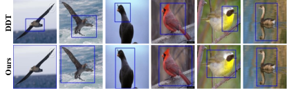
Pseudo bounding box generation. In PSOL [33], a co-supervised method DDT [26] was used to generate pseudo bounding boxes for the training set before a separate classification-regression model was trained. For comparison, we replace DDT with for bounding box generation. Following PSOL, we also adopt the resolution of when generating boxes. The input image resolution of the regression network remains . As listed in Table 6, surpasses DDT by a large margin. On ResNet50 backbone, a significant improvement of 15.6% on CUB is observed. Figure 4 shows the examples of the generated pseudo bounding boxes. DDT fails to capture the entire birds when they have long wings or tails, whereas generates accurate boxes regardless of the changes in bird scale. However, a potential drawback is that both and DDT have difficulty in dealing with the reflection, as shown in the last column.
The regression networks in prior works directly predict the coordinates of the bounding box without improving the localization map. They have difficulties in fitting pixel-wise WSOL evaluation (e.g., on OpenImages). Notably, our proposed improves the activation map before the pseudo box generation in , making CREAM applicable to both bounding box and pixel-wise evaluation.
Iterations and momentum coefficient . Tables 8 and 8 demonstrate the changes of GT-Known with different iterations and momentum coefficients . Both are conducted on . On both CUB and ILSVRC, CREAM yields the best performance when =2. CREAM (=2) outperforms CAM by nearly 30% on CUB with only 4.3-ms longer inference time per image. They have similar training time as context embedding learning is not involved in the back propagation. We visualize the re-activation maps in Figure 5. When =1, the re-activation map roughly captures the foreground object, but there are still false-positive pixels. When =2, as E-step and M-step execute in turn, the improved foreground (background) cluster centroids have a more precise indication on foreground (background), and the re-activation map is automatically refined. Nevertheless, we find that the re-activation map tends to oversmooth when is large. As shown in Table 8, CREAM is not sensitive to the momentum coefficient. A large only performs slightly better. When =1.0, the context embeddings are equivalent to randomly initialized vectors. In this case, the embeddings include much random noise in the EM process, and the performance of CREAM drops dramatically. This suggests that preserving rich context information in context embeddings helps improve the localization.
| CUB | ILSVRC | Time (s) | |
|---|---|---|---|
| 0 | 56.0 | 59.0 | 0.0017 |
| 1 | 69.3 | 65.5 | 0.0058 |
| 2 | 86.7 | 68.0 | 0.0060 |
| 3 | 82.2 | 67.0 | 0.0062 |
| 4 | 75.3 | 66.4 | 0.0065 |
| CUB | ILSVRC | |
|---|---|---|
| 0.2 | 85.2 | 67.3 |
| 0.6 | 85.4 | 67.7 |
| 0.8 | 86.7 | 68.0 |
| 0.99 | 85.6 | 67.9 |
| 1.0 | 53.1 | 60.3 |
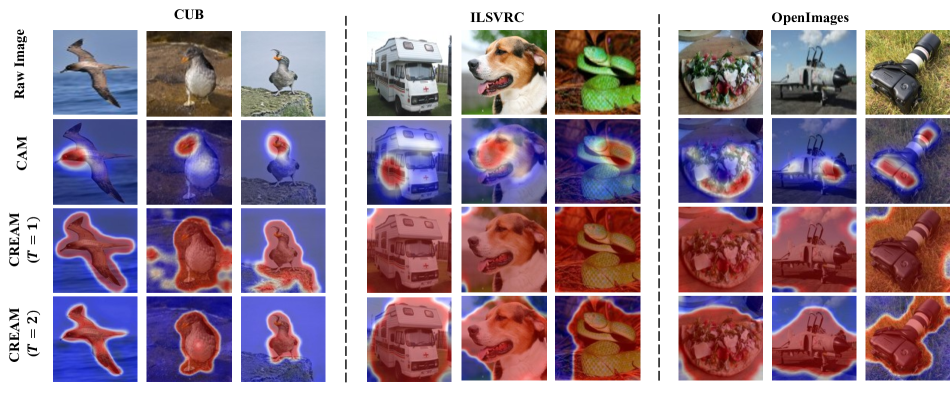
Visualization of the localization results. As shown in Figure 5, our method successfully re-activates complete foreground regions in comparison to CAM. On CUB, even embodies the capability of precise localization by highlighting the objects with a clear contour. We attribute this contour-aware localization to the EM-based re-activation. In EM process, the soft label for each pixel feature is solely determined by the similarity between the feature and the context embeddings. The pixel belongs to the foreground as long as it is more similar to the foreground context embedding than that of the background.
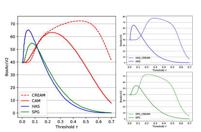
The effect of re-activation and generalization ability of CREAM. Following [5], we re-implement CAM, HAS [22] and SPG [35] on BoxAccV2 [5] using VGG16. As illustrated in Figure 6 (left), HAS and SPG perform better than CAM only when is small (e.g. <0.1). When is large (e.g. >0.2), however, there is no apparent improvement by CAM. In comparison, curve is above CAM curve for most thresholds. Besides, it is flatter around the peak, showing that is more robust to the choice of threshold.
We integrate into HAS and SPG, resulting in HAS_ and SPG_, respectively. As shown in Figure 6 (right), both HAS_ and SPG_ significantly promote the localization performance with an improvement of 10% to 60% under different thresholds. The baselines only perform better when <0.1 as their foreground activations gather around 0.1. Whereas the foreground activations in our CREAM-based counterparts appear larger. Their peaks are also more flatter than original methods. The results demonstrate the effectiveness and the generalization ability of CREAM.
6 Conclusion
In this paper, we attribute the incomplete localization problem of CAM to the mixup of the activations between less discriminative foreground regions and the background. We propose CREAM to boost the activation values of the full extent of object. A CAM-guided momentum preservation strategy is exploited to learn the class-specific context embeddings. During inference, re-activation is formulated as a parameter estimation problem and solved by a derived EM-based soft-clustering algorithm. Extensive experiments show that CREAM outperforms CAM substantially and achieves state-of-the-art results on CUB, ILSVRC and OpenImages. CREAM can be easily integrated into various WSOL approaches and boost their performance.
Acknowledgement
This work is supported by National Science and Technology Innovation 2030 - Major Project (No. 2021ZD0114001; No. 2021ZD0114000), National Natural Science Foundation of China (No. 61976057; No. 62172101), the Science and Technology Commission of Shanghai Municipality (No. 21511101000; No. 20511101203), the Science and Technology Major Project of Commission of Science and Technology of Shanghai (No. 2021SHZDZX0103).
References
- [1] Wonho Bae, Junhyug Noh, and Gunhee Kim. Rethinking class activation mapping for weakly supervised object localization. In ECCV, pages 618–634, 2020.
- [2] Soufiane Belharbi, Aydin Sarraf, Marco Pedersoli, Ismail Ben Ayed, Luke McCaffrey, and Eric Granger. F-cam: Full resolution class activation maps via guided parametric upscaling. In WACV, pages 3490–3499, 2022.
- [3] Benjamin Biggs, Oliver Boyne, James Charles, Andrew Fitzgibbon, and Roberto Cipolla. Who left the dogs out? 3d animal reconstruction with expectation maximization in the loop. In ECCV, pages 195–211, 2020.
- [4] Christopher M Bishop. Pattern recognition and machine learning. springer, 2006.
- [5] Junsuk Choe, Seong Joon Oh, Seungho Lee, Sanghyuk Chun, Zeynep Akata, and Hyunjung Shim. Evaluating weakly supervised object localization methods right. In CVPR, pages 3133–3142, 2020.
- [6] Junsuk Choe and Hyunjung Shim. Attention-based dropout layer for weakly supervised object localization. In CVPR, pages 2219–2228, 2019.
- [7] Arthur P Dempster, Nan M Laird, and Donald B Rubin. Maximum likelihood from incomplete data via the em algorithm. Journal of the Royal Statistical Society: Series B (Methodological), 39(1):1–22, 1977.
- [8] Jia Deng, Wei Dong, Richard Socher, Li-Jia Li, Kai Li, and Li Fei-Fei. Imagenet: A large-scale hierarchical image database. In CVPR, pages 248–255, 2009.
- [9] Wei Gao, Fang Wan, Xingjia Pan, Zhiliang Peng, Qi Tian, Zhenjun Han, Bolei Zhou, and Qixiang Ye. Ts-cam: Token semantic coupled attention map for weakly supervised object localization. arXiv preprint arXiv:2103.14862, 2021.
- [10] Guangyu Guo, Junwei Han, Fang Wan, and Dingwen Zhang. Strengthen learning tolerance for weakly supervised object localization. In CVPR, pages 7403–7412, 2021.
- [11] Kaiming He, Xiangyu Zhang, Shaoqing Ren, and Jian Sun. Deep residual learning for image recognition. In CVPR, pages 770–778, 2016.
- [12] Geoffrey E Hinton, Sara Sabour, and Nicholas Frosst. Matrix capsules with em routing. In ICLR, 2018.
- [13] Jeesoo Kim, Junsuk Choe, Sangdoo Yun, and Nojun Kwak. Normalization matters in weakly supervised object localization. In ICCV, pages 3427–3436, 2021.
- [14] Xia Li, Zhisheng Zhong, Jianlong Wu, Yibo Yang, Zhouchen Lin, and Hong Liu. Expectation-maximization attention networks for semantic segmentation. In ICCV, pages 9167–9176, 2019.
- [15] Weizeng Lu, Xi Jia, Weicheng Xie, Linlin Shen, Yicong Zhou, and Jinming Duan. Geometry constrained weakly supervised object localization. In ECCV, pages 481–496, 2020.
- [16] Zhekun Luo, Devin Guillory, Baifeng Shi, Wei Ke, Fang Wan, Trevor Darrell, and Huijuan Xu. Weakly-supervised action localization with expectation-maximization multi-instance learning. In ECCV, pages 729–745, 2020.
- [17] Jinjie Mai, Meng Yang, and Wenfeng Luo. Erasing integrated learning: A simple yet effective approach for weakly supervised object localization. In CVPR, pages 8766–8775, 2020.
- [18] Meng Meng, Tianzhu Zhang, Qi Tian, Yongdong Zhang, and Feng Wu. Foreground activation maps for weakly supervised object localization. In ICCV, pages 3385–3395, 2021.
- [19] Xingjia Pan, Yingguo Gao, Zhiwen Lin, Fan Tang, Weiming Dong, Haolei Yuan, Feiyue Huang, and Changsheng Xu. Unveiling the potential of structure preserving for weakly supervised object localization. In CVPR, pages 11642–11651, 2021.
- [20] Sylvia Richardson and Peter J Green. On bayesian analysis of mixtures with an unknown number of components (with discussion). Journal of the Royal Statistical Society: series B (statistical methodology), 59(4):731–792, 1997.
- [21] Karen Simonyan and Andrew Zisserman. Very deep convolutional networks for large-scale image recognition. arXiv preprint arXiv:1409.1556, 2014.
- [22] Krishna Kumar Singh and Yong Jae Lee. Hide-and-seek: Forcing a network to be meticulous for weakly-supervised object and action localization. In ICCV, pages 3544–3553, 2017.
- [23] Christian Szegedy, Vincent Vanhoucke, Sergey Ioffe, Jon Shlens, and Zbigniew Wojna. Rethinking the inception architecture for computer vision. In CVPR, pages 2818–2826, 2016.
- [24] Catherine Wah, Steve Branson, Peter Welinder, Pietro Perona, and Serge Belongie. The caltech-ucsd birds-200-2011 dataset. 2011.
- [25] Jun Wei, Qin Wang, Zhen Li, Sheng Wang, S Kevin Zhou, and Shuguang Cui. Shallow feature matters for weakly supervised object localization. In CVPR, pages 5993–6001, 2021.
- [26] Xiu-Shen Wei, Chen-Lin Zhang, Jianxin Wu, Chunhua Shen, and Zhi-Hua Zhou. Unsupervised object discovery and co-localization by deep descriptor transformation. Pattern Recognition, 88:113–126, 2019.
- [27] Yunchao Wei, Jiashi Feng, Xiaodan Liang, Ming-Ming Cheng, Yao Zhao, and Shuicheng Yan. Object region mining with adversarial erasing: A simple classification to semantic segmentation approach. In CVPR, pages 6488–6496, 2017.
- [28] Jinheng Xie, Cheng Luo, Xiangping Zhu, Ziqi Jin, Weizeng Lu, and Linlin Shen. Online refinement of low-level feature based activation map for weakly supervised object localization. In ICCV, pages 132–141, 2021.
- [29] Haolan Xue, Chang Liu, Fang Wan, Jianbin Jiao, Xiangyang Ji, and Qixiang Ye. Danet: Divergent activation for weakly supervised object localization. In ICCV, pages 6589–6598, 2019.
- [30] Shipeng Yan, Jiale Zhou, Jiangwei Xie, Songyang Zhang, and Xuming He. An em framework for online incremental learning of semantic segmentation. arXiv preprint arXiv:2108.03613, 2021.
- [31] Boyu Yang, Chang Liu, Bohao Li, Jianbin Jiao, and Qixiang Ye. Prototype mixture models for few-shot semantic segmentation. In ECCV, pages 763–778, 2020.
- [32] Sangdoo Yun, Dongyoon Han, Seong Joon Oh, Sanghyuk Chun, Junsuk Choe, and Youngjoon Yoo. Cutmix: Regularization strategy to train strong classifiers with localizable features. In ICCV, pages 6023–6032, 2019.
- [33] Chen-Lin Zhang, Yun-Hao Cao, and Jianxin Wu. Rethinking the route towards weakly supervised object localization. In CVPR, pages 13460–13469, 2020.
- [34] Xiaolin Zhang, Yunchao Wei, Jiashi Feng, Yi Yang, and Thomas S Huang. Adversarial complementary learning for weakly supervised object localization. In CVPR, pages 1325–1334, 2018.
- [35] Xiaolin Zhang, Yunchao Wei, Guoliang Kang, Yi Yang, and Thomas Huang. Self-produced guidance for weakly-supervised object localization. In ECCV, pages 597–613, 2018.
- [36] Xiaolin Zhang, Yunchao Wei, and Yi Yang. Inter-image communication for weakly supervised localization. In ECCV, pages 271–287, 2020.
- [37] Xiaolin Zhang, Yunchao Wei, Yi Yang, and Fei Wu. Rethinking localization map: Towards accurate object perception with self-enhancement maps. CoRR, abs/2006.05220, 2020.
- [38] Bolei Zhou, Aditya Khosla, Agata Lapedriza, Aude Oliva, and Antonio Torralba. Learning deep features for discriminative localization. In CVPR, pages 2921–2929, 2016.