Generalization Bounds for Gradient Methods via Discrete and Continuous Prior

Abstract

Proving algorithm-dependent generalization error bounds for gradient-type optimization methods has attracted significant attention recently in learning theory. However, most existing trajectory-based analyses require either restrictive assumptions on the learning rate (e.g., fast decreasing learning rate), or continuous injected noise (such as the Gaussian noise in Langevin dynamics). In this paper, we introduce a new discrete data-dependent prior to the PAC-Bayesian framework, and prove high probability generalization bounds of order $O(\frac{1}{n}\cdot\sum_{t=1}^{T}(\gamma_{t}/\varepsilon_{t})^{2}\left\|{\mathbf{g}_{t}}\right\|^{2})$ for floored GD and SGD (i.e. finite precision versions of GD and SGD with precision level $\varepsilon_{t}$) where, where $n$ is the number of training samples, $\gamma_{t}$ is the learning rate at step $t$, $\mathbf{g}_{t}$ is roughly the difference between the average gradient over all samples and that over only prior samples. $\left\|{\mathbf{g}_{t}}\right\|$ is upper bounded by (typically much smaller) than the gradient norm $\left\|{\nabla f(W_{t})}\right\|$. We remark that our bounds hold for nonconvex and nonsmooth loss functions. Moreover, our theoretical results provide numerically favorable upper bounds of testing errors ($0.026$ on MNIST and $0.198$ on CIFAR10). Furthermore, we study the generalization bounds for gradient Langevin Dynamics (GLD). Using the same framework with a carefully constructed continuous prior, we show a new high probability generalization bound of order $O(\frac{1}{n}+\frac{L^{2}}{n^{2}}\sum_{t=1}^{T}(\gamma_{t}/\sigma_{t})^{2})$ for GLD. The new $1/n^{2}$ rate is obtained using the concentration of the difference between the gradient of training samples and that of the prior.

1 Introduction

Bounding generalization error of learning algorithms is one of the most important problems in machine learning theory. Formally, for a supervised learning problem, the generalization error is defined as the testing error (or population error) minus the training error (or empirical error). In particular, we denote $\mathcal{R}(w,(x,y)):=\mathbbm{1}[h_{w}(x)\neq y]$ as the error of a single data point $(x,y)$, where $h_{w}(x)$ is the output of a model with parameter $w\in\mathbb{R}^{d}$. Suppose $S$ is the set of training data, each i.i.d. sampled from the population distribution $\mathcal{D}$, and we use $\mathcal{R}(w,S):=\frac{1}{|S|}\sum_{z\in S}\mathcal{R}(w,z)$ and $\mathcal{R}(w,\mathcal{D}):=\mathop{\mathbb{E}}_{z\sim D}[\mathcal{R}(w,z)]$ to denote the training error and the testing error, respectively. The generalization error of $w$ is formally defined as $\mathrm{err}_{\textrm{gen}}(w)=\mathcal{R}(w,\mathcal{D})-\mathcal{R}(w,S)$.

Proving tighter generalization bounds for general nonconvex learning and particularly deep learning has attracted significant attention recently. While the classical learning theory (uniform convergence theory) which bounds the generalization error by various complexity measures (e.g., the VC-dimension and Rademacher complexity) of the hypothesis class has been successful in several classical convex learning models, however, they become vacuous and hence fail to explain the success of modern nonconvex over-parametrized neural networks (i.e., the number of parameters significantly exceeds the number of training data) (see e.g., Zhang et al. [2017], Nagarajan and Kolter [2019]). Recently, learning theorists have tried to understand and explain generalization of deep learning from several other perspectives, such as margin theory  [Bartlett et al., 2017, Wei et al., 2019], algorithmic stability [Hardt et al., 2016, Mou et al., 2018, Li et al., 2020, Bousquet et al., 2020], PAC-bayeisan [London, 2017, Bartlett et al., 2017, Neyshabur et al., 2018, Zhou et al., 2019, Yang et al., 2019], neural tangent kernel [Jacot et al., 2018, Du et al., 2019, Arora et al., 2019, Cao and Gu, 2019], information theory [Pensia et al., 2018, Negrea et al., 2019], model compression [Arora et al., 2018, Zhou et al., 2019], differential privacy [Oneto et al., 2017, Wu et al., 2021] and so on.

In this paper, we aim to obtain tighter generalization error bounds that depend on both the training data and the optimization algorithms (a.k.a. gradient-type methods) for general nonconvex learning problems. In particular, we prove algorithm-dependent generalization bounds for several gradient-based optimization algorithms such as certain variants of gradient descent (GD), stochastic gradient descent (SGD) and stochastic gradient Langevin dynamics (SGLD). Our proofs are based on the classic Catoni’s PAC-Bayesian framework [Catoni, 2007] and also have a flavor of algorithmic stability [Bousquet and Elisseeff, 2002]. Several prior works have obtained generalization bounds for SGD and SGLD by analyzing trajectory through either the PAC-Bayesian or the algorithmic stability framework (or closely related information theoretic arguments). However, most existing results based on analyzing the optimization trajectories require either restrictive assumptions on the learning rates, or continuous noise (such as the Gaussian noise in Langevin dynamics) in order to bound the stability or the KL-divergence. In this paper, we resolve the above restrictions by combining the PAC-Bayesian framework with a few simple (yet effective) ideas, so that we can obtain new high probability and non-vacuous generalization bounds for several gradient-based optimization methods with either discrete or continuous noises (in particular certain variants of GD and SGD, either being deterministic or with discrete noise, which cannot be handled by existing techniques).

1.1 Prior work

We first briefly mention some recent work on bounding the generalization error of gradient-based methods. Hardt et al. [2016] first studied the uniform stability (hence the generalization) of stochastic gradient descent (SGD) for both convex and non-convex functions. Their results for non-convex functions requires that the learning rate $\eta_{t}$ scales with $1/t$. Their work motivates a long line of subsequent work on generalization error bounds of gradient-based optimization methods: Kuzborskij and Lampert [2018], London [2016], Chaudhari et al. [2019], Raginsky et al. [2017], Mou et al. [2018], Chen et al. [2018], Li et al. [2020], Negrea et al. [2019], Wang et al. [2021].

Recently, Simsekli et al. [2020], Hodgkinson et al. [2022] obtained generalization bound of SGD through the perspective of heavy-tailed behaviors and using the notion of Hausdorff dimension $\mathrm{d_{H}}$ which depends on both the algorithm and data.

PAC-Bayesian bounds.

The PAC-Bayesian framework [McAllester, 1999] is a powerful method for proving high probability generalization bound [Bartlett et al., 2017, Zhou et al., 2019, Mou et al., 2018]. Roughly speaking, it bounds the generalization error by the KL divergence $\mathrm{KL}\left(Q\,\big{|}\big{|}\,P\right)$, where $Q$ is the distribution of the learned output and $P$ is a prior distribution which is typically independent of dataset $S$. In this framework, bounding $\mathrm{KL}\left(Q\,\big{|}\big{|}\,P\right)$ is the most crucial part for obtaining tighter PAC-Bayesian bounds. In order to bound the KL divergence, both the prior $P$ and posterior $Q$ are typically chosen to be continuous distributions (mostly Gaussians so that KL can be computed in closed form). Hence, most prior work either considered gradient methods with continuous noise (such as Gradient Langevin Dynamics) (e.g., [Mou et al., 2018, Li et al., 2020, Negrea et al., 2019]), or injected a Gaussian noise to the final parameter at the end (e.g., [Neyshabur et al., 2018, Zhou et al., 2019]) (so $Q$ is a Gaussian distribution). We also note that designing effective prior $P$ can be also very important. For example, Lever et al. [2013] proposed to use the population distribution to compute the prior. In fact, the prior can even partially depend on the training data [Parrado-Hernández et al., 2012, Negrea et al., 2019], and our Theorem 4.1 is partially inspired by this idea.

1.2 Our contributions

First, we provide high probability generalization bounds for discrete gradient methods. In particular, we study the generalization of Floored Gradient Descent (FGD), which is a variant of GD, and Floored Stochastic Gradient Descent (FSGD), a variant of SGD. We obtain our bound by an interesting construction of discrete priors. Secondly, we consider well studied gradient methods with continuous noise, (stochastic) gradient Langvin dynamics (GLD and SGLD). We show sharper generalization bounds by carefully bounding the concentration of the sample gradients. Now, we summarize our results.

FGD and FSGD.

We first study an interesting variant of GD, called Floored GD (FGD) (Algorithm 1). The update rule of FGD is defined as follows:

$$W_{t}\leftarrow W_{t-1}-\gamma_{t}\nabla f(W_{t-1},S_{J})-\varepsilon_{t}\mathrm{floor}\left(\gamma_{t}\mathbf{g}_{t}/\varepsilon_{t}\right),$$ (FGD)

where $S_{J}$ is the subset of training dataset $S$ with size $m$ indexed by subset $J\subset[n]$ ($J$ is chosen before training), $\nabla f(W_{t-1},Z):=\frac{1}{|Z|}\sum_{z\in Z}\nabla f(W_{t-1},z)$ is the average gradient over the dataset $Z$, $\gamma_{t}$ is the learning rate, $\varepsilon_{t}$ is the precision level, and $\mathbf{g}_{t}:=\nabla f(W_{t-1},S)-\nabla f(W_{t-1},S_{J})$ is the gradient difference. The flooring operation is defined by $\mathrm{floor}(x):=\mathrm{sign}(x)\lfloor|x|\rfloor$ for any real number $x$. FGD can viewed as GD with given precision limit $\varepsilon_{t}$. We can see if we ignore the floor operation or let $\varepsilon_{t}$ approaches 0, FGD reduces to GD (see also Appendix A).

We also study a finite precision variant of SGD, called Floored SGD (FSGD) (see Section 5 for its formal definition). Empirically, the optimization and generalization capabilities of FGD and FSGD are very close to those of GD and SGD (see Figure 5 and 6 in Appendix H).

By constructing a discrete data-dependent prior and incorporate it into Catoni’s PAC-Bayesian framework, we prove that the following bound (Theorem 5.2) holds for FGD with high probability:

$$\mathcal{R}(W_{T},\mathcal{D}) \leq c_{0}\mathcal{R}(W_{T},S_{[n]\backslash J})+O\left(\frac{1}{n-m}+\frac{\ln(dT)}{n-m}\sum_{t=1}^{T}\frac{\gamma_{t}^{2}}{\varepsilon_{t}^{2}}\left\|\mathbf{g}_{t}\right\|^{2}\right),$$

where $d$ is the dimension of parameter space and $c_{0}$ can be chosen to be a small constant. The bound for FSGD is very similar (see Theorem 5.3). Now we make a few remarks about our results.

1. Our result holds for nonconvex and nonsmooth learning problems (replacing the gradients with subgradients for nonsmooth cases). Moreover, there is no additional requirement on the learning rate $\gamma_{t}$.

2. The gradient difference $\mathbf{g}_{t}$ is typical much smaller than the worst case gradient norm. It usually decreases when $m=|J|$ grows (see Figure 1(c) in Section 7).

3. We obtain non-vacuous generalization bounds on commonly used datasets. Specifically, our theoretical test error upper bounds on MNIST and CIFAR10 are $\mathbf{0.026}$ and $\mathbf{0.198}$, respectively (see Section 7). Both of them are tighter than the best-known MNIST bound ($11\%$) and CIFAR10 bound ($23\%$) reported in Dziugaite et al. [2021]. See Table 1 in Appendix B for more comparisons.

4. In order to bound the KL between $P$ and the deterministic process of FGD, we construct the prior $P$ from a discrete random processes.. We hope it may inspire future research on handling deterministic optimization algorithms or discrete noise.

Why study FGD/FSGD? We would like to remark that we study FGD/FSGD, not because FGD/FSGD have better performances than GD/SGD or other advantages. Indeed, their performances are almost the same as those of GD/SGD (see Appendix H). We use them as important stepping stones to study generalization bounds for GD and SGD. Note that most existing trajectory-based generalization bounds require either fast decreasing learning rate, or continuous injected noise, such as the Gaussian noise in Langevin dynamics, for general non-convex loss functions. Handling deterministic algorithms (such as GD) or discrete noises (such as SGD) is challenging and beyond the reach of existing techniques. In fact, understanding such discrete noises and their effects on generalization has been an important research topic (see e.g., Li et al. [2020], Zhu et al. [2019], Ziyin et al. [2021]). In particular, Zhu et al. [2019] show that it is insufficient to approximate SGD’s discrete noise by isotropic Gaussian noise. Moreover, proving nontrivial generalization bounds for SGD-like algorithms with discrete noise has also been proposed as an open research direction in Li et al. [2020].

GLD and SGLD.

We provide a new generalization bound for Gradient Langevin Dynamics (GLD). The update rule of GLD is defined as follows.

$$W_{t}\leftarrow W_{t-1}+\gamma_{t}\nabla f(W_{t-1},S)+\sigma_{t}\mathcal{N}(0,I_{d}).$$ (GLD)

In this paper, we show that the following generalization bound (Theorem 6.2) holds with high probability over the randomness of $S\sim\mathcal{D}^{n}$ and random subset $J\subset[n]$ ($|J|=m$):

$$\mathcal{R}(W_{T},\mathcal{D})\leq c_{0}\mathcal{R}(W_{T},S_{[n]\backslash J})+O\left(\frac{1}{n-m}+\frac{1}{(n-m)m}\mathop{\mathbb{E}}\left[\sum_{t=1}^{T}\frac{\gamma_{t}^{2}}{\sigma_{t}^{2}}L(W_{t-1})^{2}\right]\right),$$

where $L(W_{t-1}):=\max_{z\in S}\left\|f(W_{t-1},z)\right\|$ is the longest gradient norm of any training sample in $S$ at step $t$ and $m$ is the size of $J$. Since $W_{T}$ is independent of the index set $J$, the first term $\mathcal{R}(W_{T},S_{[n]\backslash J})$ is upper bounded by $\mathcal{R}(W_{T},S)+O(\frac{1}{\sqrt{n-m}})$ with high probability, using standard Hoeffding’s inequality. By setting $m=n/2$, our generalization bound has an $O(\frac{1}{\sqrt{n}}+\frac{1}{n}+\frac{T}{n^{2}})$ rate. The new $1/n^{2}$ rate is obtained using the concentration of the difference between the gradient of training samples and that of the prior (See Lemma 6.1).

We also prove a high probability generalization bound for Stochastic Gradient Langevin Dynamics (SGLD) (see Theorem 6.3):

$$\mathcal{R}(W_{T},\mathcal{D})\leq c_{0}\mathcal{R}(W_{T},S_{[n]\backslash J})+O\left(\frac{1}{n-m}+\frac{1}{n-m}\left(\frac{1}{b}+\frac{1}{m}\right)\mathop{\mathbb{E}}\left[\sum_{t=1}^{T}\frac{\gamma_{t}^{2}}{\sigma_{t}^{2}}L(W_{t-1})^{2}\right]\right).$$

We compare our bounds with other GLD/SGLD bounds obtained in [Mou et al., 2018, Negrea et al., 2019, Li et al., 2020] and the details can be found in Appendix B.

CLD.

Using the PAC-Bayesian framework, we obtain a new generalization bound for Continuous Langevin Dynamics (CLD), defined by the stochastic differential equation $\mathrm{d}W_{t}=-\nabla F(W_{t},S)~{}\mathrm{d}t+\sqrt{2\beta^{-1}}~{}\mathrm{d}B_{t}$. The main term of the generalization bound scales as $O(1/n^{2})$ (by choosing $m=n/2)$ and does not grow to infinity as the training time $T$ increases. See Theorem G.6 for the details.

2 Other Related Work

Stochastic Langevin Dynamics

Stochastic Langevin dynamics is a popular sampling and optimization method in machine learning [Welling and Teh, 2011]. Zhang et al. [2017], Chen et al. [2020] show a polynomial hitting time (hitting a stationary point) of SGLD in general non-convex setting. Raginsky et al. [2017] study the generalization and excess risk of SGLD in nonconvex settings and their bound depends inversely polynomially on a certain spectral gap parameter, which may be exponential small in the dimension. Continuous Langevin dynamics (SDE) with various noise structure has also been used extensively as approximations of SGD in literature (see e.g., [Li et al., 2017, 2021]). However, in terms of generalization, isotropic Gaussian noise is not a good approximation of the discrete noise in SGD (Zhu et al. [2019]).

Nonvacuous PAC-Bayesian Generalization Bounds.

Dziugaite and Roy [2017] first present a non-vacuous PAC-Bayesian generalization bound on MNIST (0.161 for a 1-layer MLP, see column T-600 of Table 1 in their paper). They use a very different training algorithm that explicitly optimizes the PAC-Bayesian bound and the output distribution is a multivariate normal distribution. To computing the closed form of KL, they choose a zero-mean Gaussian distribution as the prior distribution. Zhou et al. [2019] obtain the first non-vacuous generalization bound for ImageNet via a different method. Their method does not require any continuous noise injected but assumes that the network can be significantly compressed (so that the prior distribution is supported over the set of discrete parameters with finite precision). To our best knowledge, it is the only work that utilizes a discrete prior for proving generalization bounds of deep neural networks. Our result for FGD/FSGD has a similar flavor in a high level, that is the optimization method has a finite precision. However, our results do not need any assumption on compressibility of the model and can be applied to nonconvex learning problems other than neural networks.

Generalization bounds via Information theory.

Raginsky et al. [2017] first show that the expected generalization error $\mathop{\mathbb{E}}_{S\sim\mathcal{D}^{n}}[\mathcal{R}(W,\mathcal{D})-\mathcal{R}(W,S)]$ is bounded by $\sqrt{2I(S;W)/n}$, where $I(S;W):=\mathrm{KL}\left(P(S,W)\,\big{|}\big{|}\,P(S)\otimes P(W)\right)$ is the mutual information between the data set $S$ and the parameter $W$. This work motivates several subsequent studies [Pensia et al., 2018, Negrea et al., 2019, Bu et al., 2020, Wang et al., 2021]. The main goal in this line of work is to obtain a tight bound on the mutual information $I(S;W)$. This is again reduced to bounding the KL divergence and thus typically requires continuous injected noise (e.g., Wang et al. [2021], Negrea et al. [2019]).

3 Preliminaries

Notations.

We assume that the training dataset $S=(z_{1},..,z_{n})$ is sampled from $\mathcal{D}^{n}$, where $\mathcal{D}$ is the population distribution over the data domain $\Omega$. The model parameter $w$ is in $\mathbb{R}^{d}$. The risk function $\mathcal{R}:\mathbb{R}^{d}\times\Omega\to[0,1]$ measures the error of a model on a datapoint. The loss function $f:\mathbb{R}^{d}\times\Omega\to\mathbb{R}$ is a proxy of the risk. The optimization algorithm minimizes the loss function and we assume we can compute the gradient of the loss function. We note that the loss function may be different from the risk function (e.g., 0/1 risk vs the cross-entropy loss). The empirical risk is $\mathcal{R}(w,S)=\frac{1}{|S|}\sum_{z\in S}\mathcal{R}(w,z)$ and population risk is $\mathcal{R}(w,\mathcal{D})=\mathop{\mathbb{E}}_{z\sim\mathcal{D}}[\mathcal{R}(w,z)]$. Similarly, we can define the empirical loss $f(w,S)$ and population loss $f(w,\mathcal{D})$. For any $J=(j_{1},..,j_{m})$, we use $S_{J}$ to denote the sequence $(S_{j_{1}},...,S_{j_{m}})$. The subsequence $(A_{i},A_{i+1},...,A_{j})$ is denoted by $A_{i}^{j}$. We use $(A_{1}^{n},B_{1}^{m})$ to denote the merged sequence $(A_{1},A_{2},...,A_{n},B_{1},...,B_{m})$. When the elements in sequence $J$ are distinct, we also use $J$ to represent the set consisting of all of its elements. We may also slightly abuse the notation of a random variable to denote its distribution. For example, $\mathop{\mathbb{E}}_{x\sim X}[f(x)]$ is a shorthand for $\mathop{\mathbb{E}}_{x\sim P_{X}}[f(x)]$, and $\mathrm{KL}\left(X\,\big{|}\big{|}\,Y\right)$ means $\mathrm{KL}\left(P_{X}\,\big{|}\big{|}\,P_{Y}\right)$. For a random variable $W$, we define $\mathcal{R}(W,S)=\mathop{\mathbb{E}}_{w\sim W}[\mathcal{R}(w,S)]$ and $\mathcal{R}(W,\mathcal{D})=\mathop{\mathbb{E}}_{w\sim W}[\mathcal{R}(w,\mathcal{D})]$. The set $\{1,2,...,n\}$ is denoted by $[n]$.

KL-divergence.

Let $P$ and $Q$ be two probability distributions. The Kullback–Leibler divergence $\mathrm{KL}\left(P\,\big{|}\big{|}\,Q\right)$ is defined only when $P$ is absolute continuous with respect to $Q$ (i.e., for any $x$, $Q(x)=0$ implies $P(x)=0$). In particular, if $P$ and $Q$ are discrete distributions, then $\mathrm{KL}\left(P\,\big{|}\big{|}\,Q\right)=\sum_{x}P(x)\ln\frac{P(x)}{Q(x)}$. Otherwise, if $P$ and $Q$ are continuous distributions, it is defined as $\int P(x)\ln\frac{P(x)}{Q(x)}~{}\mathrm{d}x$. The following Lemma 3.1 is frequently used in this paper and is a well known property of KL divergence (see Cover [1999, Theorem 2.5.3], Li et al. [2020], Negrea et al. [2019]).

Lemma 3.1 (Chain Rule of KL).

We are given two random sequences $W=(W_{0},...,W_{T})$ and $W^{\prime}=(W^{\prime}_{0},...,W^{\prime}_{T})$. Then, the following equation holds (given all KLs are well defined):

$$\mathrm{KL}\left(W\,\big{|}\big{|}\,W^{\prime}\right)=\mathrm{KL}\left(W_{0}\,\big{|}\big{|}\,W^{\prime}_{0}\right)+\sum_{t=1}^{T}\mathop{\mathbb{E}}_{w\sim W_{0}^{t-1}}\left[\mathrm{KL}\left(W_{t}|W_{0}^{t-1}=w\,\big{|}\big{|}\,W^{\prime}_{t}|{W^{\prime}}_{0}^{t-1}=w\right)\right].$$

Here $W_{t}|W_{0}^{t-1}=w$ denotes the distribution of $W_{t}$ conditioning on $W_{0}^{t-1}=(W_{0},\ldots,W_{t-1})=w$.

PAC-Bayesian.

In this paper, we use the PAC-Bayesian bound presented in Catoni [2007] which enjoys a tighter $O(\mathrm{KL}\left(Q\,\big{|}\big{|}\,P\right)/n)$ rate comparing to the traditional $O(\sqrt{\mathrm{KL}\left(Q\,\big{|}\big{|}\,P\right)/n})$ bound, but with a slightly larger constant factor on the empirical error. We restate their bound as follows.

Lemma 3.2 (Catoni’s Bound).

(see e.g., Lever et al. [2013]) For any prior distribution $P$ independent of the training set $S$, any $\delta\in(0,1)$, and any $\eta>0$, the following bound holds w.p. $\geq 1-\delta$ over $S\sim\mathcal{D}^{n}$:

$$\mathop{\mathbb{E}}_{W\sim Q}[\mathcal{R}(W,\mathcal{D})] \leq\eta C_{\eta}\mathop{\mathbb{E}}_{W\sim Q}[\mathcal{R}(W,S)]+C_{\eta}\cdot\frac{\mathrm{KL}\left(Q\,\big{|}\big{|}\,P\right)+\ln(1/\delta)}{n}\quad(\forall Q),$$ (1)

where $C_{\eta}=\frac{1}{1-e^{-\eta}}$ is an absolute constant.

Concentration inequality.

We use the following variant of McDiramid inequality (Lemma 3.3) to prove the concentration of cumulative gradient difference in Section 6. The proof is deferred to Appendix C.

Lemma 3.3.

Suppose $\Phi:[n]^{m}\to\mathbb{R}^{+}$ is order-independent and $|\Phi(J)-\Phi(J^{\prime})|\leq c$ holds for any adjacent $J,J^{\prime}\in[n]^{m}$ satisfying $|J\cap J^{\prime}|=m-1$. Let $J$ be $m$ indices sampled uniformly from $[n]$ without replacement. Then $\Pr_{J}\left[\Phi(J)-\mathop{\mathbb{E}}_{J}[\Phi(J)]>\epsilon\right]\leq\exp(\frac{-2\epsilon^{2}}{mc^{2}})$.

4 Data-Dependent PAC-Bayesian Bound

The dominating term in the PAC-Bayesian bound (1) is $\mathrm{KL}\left(Q\,\big{|}\big{|}\,P\right)/n$, where $P$ is a prior distribution independent of the training dataset $S$. Typically, without knowing any information from $S$, the best possible bound for $\mathrm{KL}\left(Q\,\big{|}\big{|}\,P\right)$ we can hope is at least $\Theta(1)$ (it should not be a function of $n$ hence should not decrease with $n$). However, if we are allowed to see $m$ data points from $S$ when constructing our prior, we may produce better prediction on posterior $Q_{S}$. The following theorem enables us to use data-dependent prior in PAC-Bayesian bound. The proof is almost the same as Cantoni’s original proof and we provide a proof for completeness in Appendix D.

Theorem 4.1 (Data-Dependent PAC-Bayesian).

Suppose $J$ is a random sequence including $m$ indices uniformly sampled from $[n]$ without replacement. For any $\delta\in(0,1)$ and $\eta>0$, we have w.p. $\geq 1-\delta$ over $S\sim\mathcal{D}^{n}$ and $J$:

$$\mathcal{R}(Q,\mathcal{D})\leq\eta C_{\eta}\mathcal{R}(Q,S_{I})+C_{\eta}\cdot\frac{\mathrm{KL}\left(Q\,\big{|}\big{|}\,P(S_{J})\right)+\ln(1/\delta)}{n-m}\quad(\forall Q),$$

where $I=[n]\backslash J$ is the set of indices not in $J$, $P(S_{J})$ is the prior distribution only depending on the information of $S_{J}$ ($S_{J}$ is the subset of $S$ indexed by $J$), and $C_{\eta}:=\frac{1}{1-e^{-\eta}}$ is a constant.

Remarks. Note that the above bound holds regardless of whether $Q$ depends on $S$ or not. Also note that the first term in the right hand side is $\mathcal{R}(Q,S_{I})$, not $\mathcal{R}(Q,S)$ as in the usual generalization bounds. We remark that for most of our learning algorithms that are independent of $J$ (i.e., changing $J$ does not change the output $Q$), by standard Chernoff-Hoeffding inequality, $\mathcal{R}(Q,S_{I})$ can be bounded by $\mathcal{R}(Q,S)+O(1/\sqrt{n-m})$ with high probability over the randomness of $J$. For example, the update rules of GLD, SGLD and CLD are independent of $J$, hence $\mathcal{R}(Q,S_{I})$ can be replaced by $\mathcal{R}(Q,S)+O(1/\sqrt{n-m})$ in Theorem 4.1. However, we point out a subtle point that FGD (Algorithm 1) studied in this paper depends on $J$. It may be the case that by knowing $J$, FGD extracts more information from $S_{J}$ but not much from $S_{I}$, unintentionally making $\mathcal{R}(Q,S_{I})$ a validation error, rather than the training error as it should be. However, from our experiment (see Figure 5 and 6 in Appendix H, and Figure 2(a)), we can see that FGD is very close to GD and the $S_{I}$ error $\mathcal{R}(W_{T},S_{I})$ is indeed close to the training error $\mathcal{R}(W_{T},S)$ and both are significantly smaller than the testing error $\mathcal{R}(W_{T},\mathcal{D})$. So $\mathcal{R}(Q,S_{I})$ can be considered as a genuine training error in our study of FGD.

5 FGD and FSGD

In this section, we study the generalization error of finite precision variants of gradient descent and stochastic gradient descent: Floored Gradient Descent (FGD) and Floored Stochastic Gradient Descent (FSGD).

First we need to define the “floor” operation which is used in the definitions of FGD and FSGD.

Definition 5.1 (Floor).

For any vector $X\in\mathbb{R}^{d}$, let $Y=\mathrm{floor}(X)$ defined as:

$$Y_{i}=\mathrm{floor}(X_{i})=\lfloor X_{i}\rfloor\text{ if }X_{i}\geq 0,\quad=-\lfloor-X_{i}\rfloor\text{ if }X_{i}<0,\text{ for all }i\in[d].$$

FGD:

The Floored Gradient Descent algorithm is formally defined in Algorithm 1, where $(\gamma_{t})_{t\geq 0}$ and $(\varepsilon_{t})_{t\geq 0}$ are the step size and precision sequences, respectively. For a subset $Z\subseteq S$, we write $\nabla f(W_{t-1},Z):=\frac{1}{|Z|}\sum_{z\in Z}\nabla f(W_{t-1},z)$. Note that FGD can be viewed as gradient descent with given precision limit $\varepsilon_{t}$. We can see if we ignore the floor operation or let $\varepsilon_{t}$ approach 0, FGD reduces to the ordinary GD (see Appendix A). We also study momentum FGD, in which the 5th line of Algorithm 1 is replaced by

$$W_{t}\leftarrow W_{t-1}+\alpha\cdot\left(W_{t-1}-W_{t-2}\right)-g_{2}-\varepsilon_{t}\cdot\mathrm{floor}((g_{1}-g_{2})/\varepsilon_{t});$$

Here $\alpha>0$ is a constant. We remark that both FGD and its momentum version are deterministic algorithms. The following theorem provides the generalization error bound for both algorithms.

Input: Training dataset $S=(z_{1},..,z_{n})$. Index set $J$.

Result: Parameter $W_{T}\in\mathbb{R}^{d}$.

1 Initialize $W_{0}\leftarrow w_{0}$;

2 for $t:1\to T$ do

3       $g_{1}\leftarrow\gamma_{t}\nabla f(W_{t-1},S)$;

4       $g_{2}\leftarrow\gamma_{t}\nabla f(W_{t-1},S_{J})$;

5       $W_{t}\leftarrow W_{t-1}-g_{2}-\varepsilon_{t}\cdot\mathrm{floor}((g_{1}-g_{2})/\varepsilon_{t})$;

6      

7 end for

Algorithm 1 Floored Gradient Descent (FGD)

Theorem 5.2.

Suppose $J$ is a random sequence consisting of $m$ indices uniformly sampled from $[n]$ without replacement. Then for any $\delta\in(0,1)$, both FGD (Algorithm 1) and its momentum version satisfy the following generalization bound w.p. at least $1-\delta$ over $S\sim\mathcal{D}^{n}$ and $J$:

$$\mathcal{R}(W_{T},\mathcal{D}) \leq\eta C_{\eta}\mathcal{R}(W_{T},S_{I})+C_{\eta}\cdot\frac{\ln(1/\delta)+3}{n-m}+\frac{C_{\eta}\ln(dT)}{n-m}\sum_{t=1}^{T}\left(\frac{\gamma_{t}^{2}}{\varepsilon_{t}^{2}}\left\|\mathbf{g}_{t}\right\|^{2}\right),$$

where $d$ is the dimension of parameter space, $I=[n]\backslash J$ is the set of indices not in $J$, $C_{\eta}:=\frac{1}{1-e^{-\eta}}$ is a constant, and $\mathbf{g}_{t}:=\nabla f(W_{t-1},S)-\nabla f(W_{t-1},S_{J})$.

Proof.

We use Theorem 4.1 to prove our theorem for the momentum version. The ordinary FGD is a special case of the momentum version with $\alpha=0$. The key is to construct the prior distribution $P(S_{J})$ such that $\mathrm{KL}\left(W_{T}\,\big{|}\big{|}\,P(S_{J})\right)$ is tractable. Let $p$ be any real number in $(0,1/3)$. We first define a stochastic process $\{W^{\prime}_{0},\ldots,W^{\prime}_{T}\}$, by the following update rule ($W^{\prime}_{0}:=w_{0}$):

$$W^{\prime}_{t}\leftarrow W^{\prime}_{t-1}+\alpha\cdot\left(W^{\prime}_{t-1}-W^{\prime}_{t-2}\right)-\gamma_{t}\nabla f(W^{\prime}_{t-1},S_{J})-\varepsilon_{t}\cdot\xi_{t},$$

where $\xi_{t}$ is a discrete random variable such that for all $(a_{1},..,a_{d})\in\mathbb{Z}^{d}$:

$$\Pr[\xi_{t}=(a_{1},...,a_{d})^{\top}]:=\left(\sum_{i=-\infty}^{\infty}p^{i^{2}}\right)^{-d}\exp\left(-\sum_{k=1}^{d}\ln(1/p)a_{k}^{2}\right).$$

It is easy to verify that the sum of the probabilities ($\sum_{a\in\mathbb{Z}^{d}}\Pr[\xi_{t}=a]$) equals to $1$. Note that $W^{\prime}_{t}$ only depends on $S_{J}$. We define $P(S_{J})$ as the distribution of $W^{\prime}_{T}$.

Recall that $W_{0}^{t}=(W_{0},...,W_{t})$ is the parameter sequence of FGD (Algorithm 1). Applying the chain rule of KL-divergence (Lemma 3.1), we have:

$$\begin{split}\mathrm{KL}\left(W_{T}\,\big{|}\big{|}\,P(S_{J})\right)&=\mathrm{KL}\left(W_{T}\,\big{|}\big{|}\,W^{\prime}_{T}\right)\leq\mathrm{KL}\left(W_{0}^{T}\,\big{|}\big{|}\,{W^{\prime}}_{0}^{T}\right)\\ &=\sum_{t=1}^{T}\mathop{\mathbb{E}}_{w\sim W_{0}^{t-1}}\left[\mathrm{KL}\left(W_{t}|W_{0}^{t-1}=w\,\big{|}\big{|}\,W^{\prime}_{t}|{W^{\prime}}_{0}^{t-1}=w\right)\right]\\ &=\sum_{t=1}^{T}\mathrm{KL}\left(W_{t}|W_{0}^{t-1}=W_{0}^{t-1}\,\big{|}\big{|}\,W^{\prime}_{t}|{W^{\prime}}_{0}^{t-1}=W_{0}^{t-1}\right).\\ \end{split}$$ (2)

The last equation holds because FGD is deterministic. Let $w=W_{0}^{t-1}$. The distribution of $W_{t}|W_{0}^{t-1}=w$ (where $w=(w_{0},...,w_{t-1})$) is a point mass on

$$w_{t-1}+\alpha\cdot\left(w_{t-1}-w_{t-2}\right)-\gamma_{t}\nabla f(w_{t-1},S_{J})-\varepsilon_{t}\cdot\mathrm{floor}\left(\frac{\gamma_{t}(\nabla f(w_{t-1},S)-\nabla f(w_{t-1},S_{J}))}{\varepsilon_{t}}\right).$$

Let vector $a=(a_{1},\ldots,a_{d})=\mathrm{floor}(\frac{\gamma_{t}}{\varepsilon_{t}}(\nabla f(w_{t-1},S)-\nabla f(w_{t-1},S_{J})))$. By the definition of $W^{\prime}_{t}$, we have

$$\mathrm{KL}\left(W_{t}|W_{0}^{t-1}=w\,\big{|}\big{|}\,W^{\prime}_{t}|{W^{\prime}}_{0}^{t-1}=w\right)=1\cdot\ln\left(1/\Pr\left[\xi_{t}=a\right]\right)$$

$$=\ln\left(\Bigl{(}\sum_{i=-\infty}^{\infty}p^{i^{2}}\Bigr{)}^{d}\right)+\sum_{k=1}^{d}\ln(1/p)\cdot a_{k}^{2}.$$

Since $|i|\leq i^{2}$ and $p\in(0,1/3)$, we have $\ln\left((\sum_{i=-\infty}^{\infty}p^{i^{2}})^{d}\right)$ is at most $d\ln\left(1+2\sum_{i=1}^{\infty}p^{i}\right)$. It can be further bounded by $d\ln\left(1+3p\right)$. Moreover, it can be bounded by $3dp$ as $\ln(1+x)\leq x$. Thus, the above KL-divergence can be bounded by $3dp+\sum_{k=1}^{d}\ln(1/p)a_{k}^{2}$. Recall that the $k$th entry of $a$ is $a_{k}:=\lfloor\frac{\gamma_{t}}{\varepsilon_{t}}\cdot(\nabla_{k}f(w_{t-1},S)-\nabla_{k}f(w_{t-1},S_{J}))\rfloor$, which is less than or equal to $\frac{\gamma_{t}}{\varepsilon_{t}}\cdot(\nabla_{k}f(w_{t-1},S)-\nabla_{k}f(w_{t-1},S_{J}))$. Therefore, we have

$$\mathrm{KL}\left(W_{t}|W_{0}^{t-1}=w\,\big{|}\big{|}\,W^{\prime}_{t}|{W^{\prime}}_{0}^{t-1}=w\right)\leq 3dp+\frac{\ln(1/p)\gamma_{t}^{2}}{\varepsilon_{t}^{2}}\left\|\nabla f(w_{t-1},S)-\nabla f(w_{t-1},S_{J})\right\|_{2}^{2}.$$

Plugging the above inequality into (2), we have

$$\mathrm{KL}\left(W_{T}\,\big{|}\big{|}\,P(S_{J})\right) \leq\sum_{t=1}^{T}\left(3dp+\frac{\ln(1/p)\gamma_{t}^{2}}{\varepsilon_{t}^{2}}\left\|\nabla f(W_{t-1},S)-\nabla f(W_{t-1},S_{J})\right\|_{2}^{2}\right).$$

We conclude our proof by plugging it into Theorem 4.1 (setting $p=1/(Td)$). ∎

FSGD:

We can use a similar approach to prove a generalization bound for Floored Stochastic Gradient Desent (FSGD). Formally, FSGD is identical to Algorithm 1 except for the definitions of $g_{1}$ and $g_{2}$ replaced with:

$$g_{1}\leftarrow\nabla f(W_{t-1},S_{B_{t}}),\quad g_{2}\leftarrow\nabla f(W_{t-1},S_{B_{t}\cap J}),$$

where $B_{t}\subseteq[n]$ is a random batch independent of $S,J$ and $W_{0}^{t-1}$. Formally, each $B_{t}$ is a set including $b$ indices uniformly sampled from $[n]$ without replacement. The following theorem provides a generalization bound for FSGD. The proof can be found in Appendix E.

Theorem 5.3.

Suppose $J$ is a random sequence consisting of $m$ indices uniformly sampled from $[n]$ without replacement. Then for any $\delta\in(0,1),\varepsilon\in(0,1)$, FSGD satisfies the following generalization bound: w.p. at least $1-\delta$ over $S\sim\mathcal{D}^{n}$ and $J$:

$$\mathcal{R}(W_{T},\mathcal{D}) \leq\eta C_{\eta}\mathcal{R}(W_{T},S_{I})+C_{\eta}\cdot\frac{\ln(1/\delta)+3}{n-m}+\frac{C_{\eta}\ln(dT)}{n-m}\mathop{\mathbb{E}}_{B_{0}^{T}}\left[\sum_{t=1}^{T}\frac{\gamma_{t}^{2}}{\varepsilon_{t}^{2}}\left\|\mathbf{g}_{t}\right\|^{2}\right],$$

where $d$ is the dimension of parameter space, $I=[n]\backslash J$, $C_{\eta}:=\frac{1}{1-e^{-\eta}}$ is a constant, and $\mathbf{g}_{t}:=f(W_{t-1},S_{B_{t}})-\nabla f(W_{t-1},S_{J\cap B_{t}})$.

6 Gradient Langevin Dynamics

In this section, we present new generalization bounds for Gradient Langevin Dynamics (GLD) and Stochastic Gradient Langevin Dynamics (SGLD) based on Theorem 4.1.

Gradient Langevin Dynamics (GLD):

The GLD algorithm can be viewed as gradient descent plus a Gaussian noise. Formally, for a given training set $S\sim\mathcal{D}^{n}$, the update rule of GLD is defined as follows:

$$W_{t+1}\leftarrow W_{t}-\frac{\gamma_{t+1}}{n}\sum_{z\in S}\nabla f(W_{t},z)+\sigma_{t+1}\mathcal{N}(0,I_{d}),$$ (GLD)

Here the gradient $\nabla f(W_{t},z)$ can be replaced with any gradient-like vector such as a clipped gradient. The output of GLD is the last step parameter $W_{T}$ or some function of the whole training trajectory $W_{0}^{T}$ (e.g., the average of the suffix $\frac{1}{K}\sum_{t=T-K}^{T}W_{t}$).

We still use the data-dependent PAC-Bayesian framework (Theorem 4.1) to prove the generalization bound for GLD. Unlike FGD (Algorithm 1), GLD is independent of the prior indices $J$, which enables us to prove the following concentration bound (Lemma 6.1) for the gradient difference. The proof is based on Lemma 3.3, which is postponed to Appendix F.

Lemma 6.1.

Let $S=(z_{1},...z_{n})$ be any fixed training set. $J$ is a random sequence including $m$ indices uniformly sampled from $[n]$ without replacement, and $W=(W_{0},...,W_{T})$ is any random sequence independent of $J$. Then the following bound holds with probability at least $1-\delta$ over the randomness of $J$:

$$\mathop{\mathbb{E}}_{W}\left[\sum_{t=1}^{T}\frac{\gamma_{t}^{2}}{\sigma_{t}^{2}}\left\|\nabla f(W_{t-1},S)-\nabla f(W_{t-1},S_{J})\right\|^{2}\right]\leq\frac{C_{\delta}}{m}\mathop{\mathbb{E}}_{W}\left[\sum_{t=1}^{T}\frac{\gamma_{t}^{2}}{\sigma_{t}^{2}}L(W_{t-1})^{2}\right],$$

where $C_{\delta}=4+2\ln(1/\delta)+5.66\sqrt{\ln(1/\delta)}$, and $L(w)=\max_{i\in[n]}\left\|\nabla f(w,z_{i})\right\|$.

Now we are ready to present our main results. The proofs can be found in Appendix F.

Theorem 6.2.

Suppose $J$ is a random sequence consisting of $m$ indices uniformly sampled from $[n]$ without replacement. Let $W_{T}$ be the output of GLD. Then for any $\delta\in(0,\frac{1}{2})$ and $\eta>0$, we have w.p. $\geq 1-2\delta$ over $S\sim\mathcal{D}^{n}$ and $J$, the following holds ($L(w):=\max_{z\in S}\left\|f(w,z)\right\|$):

$$\mathcal{R}(W_{T},\mathcal{D})\leq\eta C_{\eta}\mathcal{R}(W_{T},S_{I}) +\frac{C_{\eta}\ln(1/\delta)}{n-m}+\frac{C_{\eta}C_{\delta}}{2(n-m)m}\mathop{\mathbb{E}}_{W_{0}^{T}}\left[\sum_{t=1}^{T}\frac{\gamma_{t}^{2}}{\sigma_{t}^{2}}L(W_{t-1})^{2}\right],$$

where $C_{\delta}=4+2\ln(1/\delta)+5.66\sqrt{\ln(1/\delta)}$, $I=[n]\backslash J$ and $C_{\eta}=\frac{1}{1-e^{-\eta}}$.

Stochastic Gradient Langevin Dynamics (SGLD):

For a given training data set $S$, the update rule of SGLD is defined as:

$$W_{t+1}\leftarrow W_{t}-\gamma_{t+1}\nabla f(W_{t},S_{B_{t}})+\sigma_{t+1}\mathcal{N}(0,I_{d}),$$ (SGLD)

where $B_{t}\sim\mathrm{uniform}([n])^{b}$ is the mini-batch of size $b$ at step $t$. Note that $B_{t}$ is a sequence instead of a set, thus it may include duplicate elements. Similar to the analysis of GLD, we can prove the following bound for SGLD.

Theorem 6.3.

Let $W_{T}$ be the output of SGLD when the training set is $S$, and $J$ be a random sequence with $m$ indices uniformly sampled from $[n]$ without replacement. For any $\delta\in(0,1)$ and $m\geq 1$, we have w.p. $\geq 1-2\delta$ over $S\sim\mathcal{D}^{n}$ and $J$, the following holds:

$$\mathcal{R}(W_{T},\mathcal{D})\leq\eta C_{\eta}\mathcal{R}(W_{T},S_{I})+\frac{C_{\eta}\ln(1/\delta)}{n-m}+\frac{C_{\eta}}{n-m}\left(\frac{4}{b}+\frac{C_{\delta}}{2m}\right)\mathop{\mathbb{E}}_{W_{0}^{T}}\left[\sum_{t=1}^{T}\frac{\gamma_{t}^{2}}{\sigma_{t}^{2}}L(W_{t-1})^{2}\right],$$

where $L(w):=\max_{z\in S}\left\|f(w,z)\right\|$, $C_{\delta}=4+2\ln(1/\delta)+5.66\sqrt{\ln(1/\delta)}$, $C_{\eta}=\frac{1}{1-e^{-\eta}}$, $b$ is the batch size, and $I=[n]\backslash J$.

Remark 6.4.

If the gradient norm is bounded and we use a decaying learning rate schedule such as $\gamma_{t}\propto O(1/t)$, then the summation in our bound converges. Hence, under such a learning rate schedule, Theorem 6.2 and  6.3 imply the following test error bound for GLD or SGLD: $\mathcal{R}(W_{T},\mathcal{D})\leq\eta C_{\eta}\mathcal{R}(W_{T},S_{I})+\widetilde{O}(\frac{1}{n-m})$ which is independent of $T$, where $\widetilde{O}$ hides some logarithmic factors.

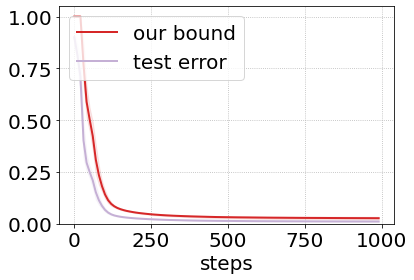
(a) entire training path

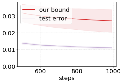
(b) later stage

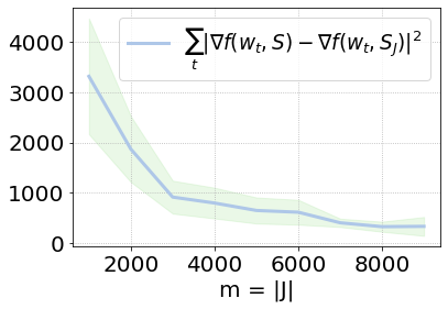
(c) gradient difference

Figure 1: MNIST + CNN + FGD. In (a) and (b), we plot the true test error and our bound (Theorem 5.2 with $\eta=1.5,\delta=0.1$). In (c), we show how cumulative gradient difference decreases as $m$ (the size of $J$) increases.

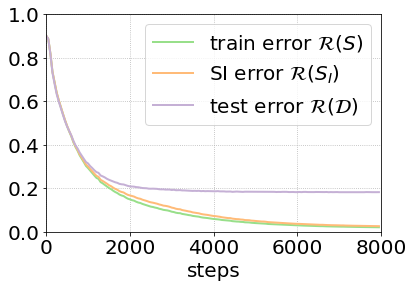
(a) training and test errors (FSGD)

(b) our bound

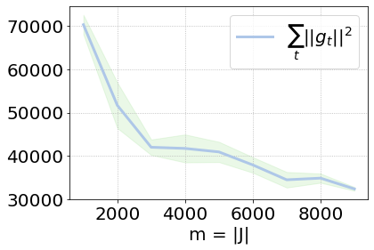
(c) gradient difference

Figure 2: CIFAR10 + SimpleNet + FSGD. In (a), we plot $\mathcal{R}(W_{T},S_{I})$, $\mathcal{R}(W_{T},S)$ and the test error. We can see that $\mathcal{R}(W_{T},S_{I})$ is very close to $\mathcal{R}(W_{T},S)$. In (b), we plot our theoretical bound (Theorem 5.3 with $\eta=2,\delta=0.1$). The red part corresponds to the first term of our bound (the empirical risk) and the green part corresponds to the rest. The last step test error and our bound are $0.18$ and $\mathbf{0.198}$, respectively. In (c), we show how cumulative gradient difference decreases as $m$ (the size of $J$) increases.

7 Experiment

In this section, we conduct experiments for FGD and FSGD on MNIST [LeCun et al., 1998] and CIFAR10 [Krizhevsky et al., 2009] to investigate the the optimization and generalization properties of FGD and FSGD, and the numerical closeness between our theoretical bounds and true test errors. Due to space limit, the detailed experimental setting and some additional experimental results can be found in Appendix H.

FGD/FSGD vs GD/SGD.

We first demonstrate that the training and testing curves of FGD and GD are nearly identical (we choose precision level $\varepsilon=0.005$ or $0.004$). We also show that the same is true for FSGD vs SGD. Due to space limit, the figures are presented in Appendix H (Figure 5 and 6).

Non-vacuous bounds.

For MNIST, we train a CNN ($d=1.4\cdot 10^{6}$) by FGD with $\gamma_{t}=0.005\cdot 0.9^{\lfloor\frac{t}{150}\rfloor}$ and $\varepsilon_{t}=0.005$ and momentum $\alpha=0.9$). The size $m=|J|$ is set to $n/2=30000$. As shown in Figure 1(a) and 1(b), our bound (Theorem 5.2 with $\eta=1.5,\delta=0.1$) tracks the testing error closely. At step $T=990$, our bound is $\mathbf{0.026}$ while the testing error is $0.011$. This is non-vacuous and tighter than best known $11\%$ MNIST bound reported in Dziugaite et al. [2021]. For CIFAR10, we train a SimpleNet [Hasanpour et al., 2016] without BatchNorm and Dropout. The number of parameters $d$ is nearly $18\cdot 10^{6}$. We use FSGD to train our model. The learning rate $\gamma_{t}$ is set to $0.001\cdot 0.9^{\lfloor t/200\rfloor}$, the precision $\varepsilon_{t}$ is set to $0.004$, and the momentum $\alpha$ is set to $0.99$. The batch size is $2000$. $m=|J|$ is set to $n/5=10000$. The result is shown in Figure 2(b). We stop training at step $t=8000$ when the testing error is and $0.18$. At that time, our testing error bound is $\mathbf{0.198}$ which is non-vacuous and tighter than best known ${0.23}$ CIFAR10 bound reported in Dziugaite et al. [2021].

Decrease of the gradient difference.

Intuitively, the cumulative squared norm of gradient difference $\mathbf{g}_{t}:=\nabla f(W_{t},S)-\nabla f(W_{t},S_{J})$ should decrease as $m=|J|$ increases. Although we cannot prove a concentration like Lemma 6.1 (i.e., $\left\|\mathbf{g}_{t}\right\|^{2}$ scales as $O(1/m)$), we can still observe that $\left\|\mathbf{g}_{t}\right\|^{2}$ decreases when $m$ increases. The results are depicted in Figure 1(c) and Figure 2(c).

Random labels.

We conduct the random label experiment designed in Zhang et al. [2017]. Our theoretical bounds can distinguish the datasets with different portion ($p$) of random labels. See Appendix H.

8 Conclusion

In this paper, we prove new generalization bounds for several gradient-based methods with either discrete or continuous noises based on carefully constructed data-dependent priors. Recall that FGD requires to compute the gradient difference for technical reasons. It would be more natural and desirable if we only need to compute the full gradient and rounded to the nearest grid point. An intriguing future direction is to free FGD/FSGD from the dependence of the prior subset $J$ so that we can apply the concentration on the gradient difference to obtain a tighter bound. Of course, a major further direction is to obtain similar generalization bounds for vanilla GD and SGD, which remains to be an important open problem in this line of work. Our technique can be useful for handling deterministic algorithms and discrete noises, but it seems that new technical ideas or assumptions are needed for tackling GD or SGD.

9 Acknowledgements

The authors would like to thank the anonymous reviewers for their constructive comments. The authors are supported in part by the National Natural Science Foundation of China Grant 62161146004, Turing AI Institute of Nanjing and Xi’an Institute for Interdisciplinary Information Core Technology.

Appendix A Floored Gradient Descent

FGD is a finite precision variant of GD. It decomposes the full gradient $g_{1}:=\gamma_{t}\nabla f(W_{t},S)$ (used in GD) into a sum of two parts, $g_{2}:=\gamma_{t}\nabla f(W_{t},S_{J})$ and $\Delta g:=\gamma_{t}(g_{1}-g_{2})=\gamma_{t}\nabla f(W_{t},S)-\gamma_{t}\nabla f(W_{t},S_{J})$, where $J\subseteq[n]$ is a subset fixed before training and $S_{J}$ is the subset of training data corresponding to index set $J$. Note that $S_{J}$ is the “prior" dataset, rather than a mini-batch. Then we reduce the precision of $\Delta g$ to $\varepsilon_{t}$ by applying a floor-operation $\Delta^{\prime}g:=\varepsilon_{t}\mathrm{floor}(\Delta g/\varepsilon_{t})$. Hence, $g_{2}+\Delta^{\prime}g$ can be viewed as an approximation of full gradient $g_{1}=g_{2}+\Delta g$.

It is easy to see that if we ignore the floor operation or when $\varepsilon_{t}$ goes to $0$, FGD becomes GD. More concretely, recall that the update rule of FGD is (WLOG let $\gamma_{t}=1$):

$$W_{t}\leftarrow W_{t-1}-\nabla f(W_{t-1},S_{J})-\varepsilon_{t}\cdot\mathrm{floor}\left(\frac{\nabla f(W_{t-1},S)-\nabla f(W_{t-1},S_{J})}{\varepsilon_{t}}\right).$$

(1) If we ignore the floor operation in the last term, the equation becomes

$$W_{t} \leftarrow W_{t-1}-\nabla f(W_{t-1},S_{J})-\varepsilon_{t}\cdot\left(\frac{\nabla f(W_{t-1},S)-\nabla f(W_{t-1},S_{J})}{\varepsilon_{t}}\right)$$

$$=W_{t-1}-\nabla f(W_{t-1},S_{J})-(\nabla f(W_{t-1},S)-\nabla f(W_{t-1},S_{J}))$$

$$=W_{t-1}-\nabla f(W_{t-1},S).$$

(2) When $\varepsilon\rightarrow 0$, it is easy to see that $\lim_{\varepsilon\rightarrow 0}\varepsilon\cdot\mathrm{floor}(x/\varepsilon)=x$. Again, the FGD update rule reduces to

$$W_{t} \leftarrow W_{t-1}-\nabla f(W_{t-1},S_{J})-(\nabla f(W_{t-1},S)-\nabla f(W_{t-1},S_{J}))$$

$$=W_{t-1}-\nabla f(W_{t-1},S).$$

The contribution of $\nabla f(W_{t-1},S_{J})$ is canceled out, and again FGD becomes GD.

Appendix B Comparison with Existing Work

B.1 Numerical bounds on MNIST and CIFAR10

The following table (Table 1) lists some of existing theoretical test bounds for MNIST and CIFAR10. Typically, for both datasets, one can fit the training set very well and obtain a near zero training error. Hence, the generalization error bound is quite close to the theoretical test error bound. There is no numerical experiment in Mou et al. [2018] and the number is excerpted from Negrea et al. [2019]. The first few rows are excerpted from Nagarajan and Kolter [2017].

Reference	Algorithms	Approach	MNIST	CIFAR10
Harvey et al. [2017]	Any	VC-dim	large	large
Bartlett et al. [2017]	Any	Margin-based	large	large
Golowich et al. [2018]	Any	Rademacher Complexity	large	large
Arora et al. [2018]	Any	Compression	-	large
Dziugaite and Roy [2017]	OPT-PAC	PAC-Bayes	0.161	-
Mou et al. [2018]	SGLD	PAC-Bayes	$\approx$ 1.2	-
Li et al. [2020]	GLD/SGLD	Bayes-Stability	$\approx$ 0.2	$\approx$ 207
Zantedeschi et al. [2021]	Majority Votes	PAC-Bayes	$\approx$ 0.45	-
Zhou et al. [2019]	Any	PAC-Bayes	0.46	-
Negrea et al. [2019]	SGLD	Information theory	0.21	41.13
Haghifam et al. [2020]	SGLD	Information theory	$\approx$ 0.15	$\approx$ 0.72
Dziugaite et al. [2021]	OPT-PAC	PAC-Bayes	0.11	0.23
Our bound	FGD/FSGD	PAC-Bayes	0.026	0.198

Table 1: Comparison with existing theoretical upper bounds of test errors on MNIST and CIFAR10. “Any” means that the bound only depends on the trained network, not the training algorithm. “OPT-PAC" means that the work optimizes a different loss function that corresponds to the PAC-Bayesian bound. “large” means that the bound is far greater than 1 and “-” indicates the bound is not reported in that paper.

B.2 Comparison with Existing GLD/SGLD bounds

We compare our bounds for GLD/SGLD (Theorem 6.2 and 6.3) with existing GLD/SGLD generalization bounds in prior work. For GLD, Mou et al. [2018] provide a generalization bound in expectation based on the uniform stability framework, which is of rate $O(\frac{L\sqrt{T}}{n})$, where $L$ is the global Lipschitz constant (ignoring the factors depending on $\gamma_{t}$ and $\sigma_{t}$). Their bound can be tighten to $O(\frac{1}{n}\sqrt{\sum_{t=1}^{T}L^{2}_{t}})$ where $L_{t}$ is the gradient norm at time $t$ (which is always less than $L$)  [Li et al., 2020]. Their bounds can be converted to high probability bound with an additional factor $O(1/\sqrt{n})$ using the technique developed in [Feldman and Vondrak, 2019]. Bounds of similar orders have been also obtained through information theory [Wang et al., 2021, Haghifam et al., 2020] and differential privacy [Wu et al., 2021]. Note that the main term in our bound is of order $O(\frac{1}{n^{2}}\sum_{t=1}^{T}L^{2}_{t})$, which is quadratically better than theirs if the bound is in $(0,1)$. For SGLD, Mou et al. [2018] and Li et al. [2020] obtained similar bounds, but requires the assumption that the learning rate should be of order $O(1/L)$. Our bound for SGLD does not require such assumption and is more favorable for large minibatch size $b$. For small value of $b$ (say $b=O(1)$), our bound can be worse.

Another closely related work is Negrea et al. [2019]. They also use a data-dependent prior and present an in-expectation bound based on information theory. They introduce a quantity called “incoherence” $\left\|\xi_{t}\right\|$ that is defined somewhat similar to $\|\mathbf{g}_{t}\|$ (it is also the norm of the different between two gradients defined by two different subsets of samples). They obtained an $O(\sqrt{\frac{1}{n-m}\sum_{t=1}^{T}\frac{\gamma_{t}^{2}}{\sigma_{t}^{2}}\mathop{\mathbb{E}}[\left\|\xi_{t}\right\|^{2}]})$ bound for SGLD. By taking expectation, it can be further bounded by $O(\sqrt{\frac{1}{n}\sum_{t=1}^{T}(\frac{1}{b}+\frac{(n-m)}{nm})\frac{\gamma_{t}^{2}}{\sigma_{t}^{2}}V_{t}})$, where $V_{t}$ is a quantity about the same size as the variance of training gradients. In fact, they obtain a worst case $O(\frac{(n-m)^{2}}{n^{2}}\sum_{t=1}^{T}\frac{L^{2}\gamma_{t}^{2}}{\sigma_{t}^{2}})$ bound for $\mathrm{KL}\left(Q\,\big{|}\big{|}\,P(S_{J})\right)$, and if we plug it into Catoni’s PAC-Bayesian bound (Theorem 4.1), one can obtain an $O(\frac{1}{n-m}+\frac{(n-m)}{n^{2}}\sum_{t=1}^{T}\frac{\gamma_{t}^{2}}{\sigma_{t}^{2}}L^{2})$ high probability bound (see Theorem B.1 below for details). To make the 2nd term in their bound have the same $O(1/n^{2})$ rate as ours, one needs to set $n-m=O(1)$ which would result in a large first term $\frac{1}{n-m}=\Omega(1)$. Moreover, our construction of data-dependent prior $P(S_{J})$ is also very different from theirs. Their idea is to use the gradients in $S_{J}$ to cancel out the gradients in $S$ while ours is based on the property that the mean gradient on $S_{J}$ is concentrated around the mean gradient of the whole dataset $S$.

Theorem B.1.

Suppose the loss $f$ is $L$-Lipschitz (i.e., $\left\|\nabla f(w,z)\right\|\leq L$ holds for all $w,z$). Then for GLD, we have the following bound holds w.p. at least $1-\delta$ over the randomness of $J$ and $S\sim\mathcal{D}^{n}$:

$$\mathcal{R}(W_{T},\mathcal{D})\leq\eta C_{\eta}\mathcal{R}(W_{T},S_{[n]\backslash J})+O\left(\frac{\ln(1/\delta)}{n-m}+\frac{(n-m)}{n^{2}}\sum_{t=1}^{T}\frac{\gamma_{t}^{2}}{\sigma_{t}^{2}}L^{2}\right),$$

where $C_{\eta}=\frac{1}{1-e^{-\eta}}$.

Proof.

Using a data-dependent prior $P(S_{J})$ defined in Negrea et al. [2019, Section 3.1.1], one can obtain an $O(\frac{(n-m)^{2}}{n^{2}}\sum_{t=1}^{T}\frac{\gamma_{t}^{2}}{\sigma_{t}^{2}}L^{2})$ bound for $\mathrm{KL}\left(W_{T}\,\big{|}\big{|}\,P(S_{J})\right)$ (see Negrea et al. [2019, Section 3.1.1] for details). We conclude the proof by plugging it into Theorem 4.1. ∎

Mou et al. [2018] also obtain a high probability PAC-Bayesian bound of rate $O(\sqrt{\frac{1}{n}\sum_{t=1}^{T}e^{-r_{t}}L_{t}^{2}})$ if there is an $\ell_{2}$-regularization in the loss (ignoring other factors depending on $\gamma_{t}$ and $\sigma_{t}$). Here $e^{-r_{t}}<1$ is a decay factor depending on the regularization coefficient. There is a similar decay factor in Wang et al. [2021]’s bound (the fact comes from strong data processing inequalities). Note that without $\ell_{2}$-regularization, there is no such decay factor, and Mou et al. [2018]’s bound becomes $O(\sqrt{T/n})$, which is looser than ours. From technical perspective, they use Fokker Planck equation to track the time derivative of KL and Logarithmic Sobolev inequality to related KL with Fisher information. We also use these tools for our generalization bound of Continuous Langevin dynamics (CLD) (see Appendix G), but the general proof idea is very different.

Appendix C Omitted Proofs in Section 3

In this section, we are going to prove a generalized McDiarmid’s inequality (Lemma 3.3). To avoid frequently writing long expression $\Phi(j_{1},j_{2},...,j_{i},J_{i+1},...,J_{m})$, we briefly denoted it as $\Phi(j_{1}^{i},J_{i+1}^{m})$, where $j_{l}^{r}$ is a abbreviation of sequence $(j_{l},j_{l+1},...,j_{r})$. Before proving it, we need the following lemma:

Lemma C.1 (Theorem 5.3 in Dubhashi and Panconesi [2009]).

Let $J=(J_{1},...,J_{m})$ be any random sequence and $\Phi$ be a function of $J$. If for any $i\in[m]$ and any fixed $j_{1}^{i}=(j_{1},..,j_{i})$, it satisfies

$$\left|\mathop{\mathbb{E}}_{J_{i+1}^{m}}[\Phi(j_{1}^{i},J_{i+1}^{m})|J_{1}^{i}=j_{1}^{i}]-\mathop{\mathbb{E}}_{J_{i}^{m}}[\Phi(j_{1}^{i-1},J_{i}^{m})|J_{1}^{i-1}=j_{1}^{i-1}]\right|\leq c_{i}.$$

Then, the following inequality holds:

$$\Pr_{J}\left[\Phi(J)-\mathop{\mathbb{E}}_{J}[\Phi(J)]>\epsilon\right]\leq\exp\left(-\frac{2\epsilon^{2}}{\sum_{i=1}^{m}c_{i}^{2}}\right).$$

Now we are able to prove our result.

Lemma.

3.3  Suppose $\Phi:[n]^{m}\to\mathbb{R}^{+}$ is order-independent and $|\Phi(J)-\Phi(J^{\prime})|\leq c$ holds for any adjacent $J,J^{\prime}\in[n]^{m}$ satisfying $|J\cap J^{\prime}|=m-1$. Let $J$ be $m$ indices sampled uniformly from $[n]$ without replacement. Then $\Pr_{J}\left[\Phi(J)-\mathop{\mathbb{E}}_{J}[\Phi(J)]>\epsilon\right]\leq\exp(\frac{-2\epsilon^{2}}{mc^{2}})$.

Proof.

It suffices to verify that the conditions in Lemma C.1 are satisfied. For any fixed $j_{1}^{i}=(j_{1},...,j_{i})$, let $X$ and $Y$ be two independent random variables with distribution equal to $J|J_{1}^{i}=j_{1}^{i}$ and $J|J_{1}^{i-1}=j_{1}^{i-1}$, respectively.

The goal is to find an upper bound $c_{i}$ for $|\mathop{\mathbb{E}}[\Phi(X)]-\mathop{\mathbb{E}}[\Phi(Y)]|$. We distinguish the following disjoint events.

• $\mathcal{E}_{1}:Y_{i}=j_{i}$.
  Conditioning on this, we have $X_{i+1}^{m}$ and $Y_{i+1}^{m}$ share the same distribution. Notice that $X_{1}^{i}=Y_{1}^{i}$. Thus, we have:

  $$|\mathop{\mathbb{E}}[\Phi(X)-\Phi(Y)\,\,\,|\,\,\mathcal{E}_{1}]|=0.$$

• $\mathcal{E}_{2}:Y_{i}\neq j_{i}\quad\bigcap\quad Y_{i}\notin X_{i+1}^{m}\quad\bigcap\quad j_{i}\notin Y_{i+1}^{m}$.
  Conditioning on this, both suffixes $X_{i+1}^{m}$ and $Y_{i+1}^{m}$ are sampled from $[n]\backslash(j_{1}^{i}\cup J^{\prime}_{i})$. Thus their distributions are identical. We have

  $$|\mathop{\mathbb{E}}[\Phi(X)|\mathcal{E}_{1}] -\mathop{\mathbb{E}}[\Phi(Y)|\mathcal{E}_{2}]|$$

  $$\leq\mathop{\mathbb{E}}_{j_{i+1}^{m}\sim X_{i+1}^{m}}[|\Phi(j_{1}^{i-1},j_{i},j_{i+1}^{m})-\Phi(j_{1}^{i-1},Y_{i},j_{i+1}^{m})|]$$

  $$\leq c.$$ (Assumption)

• $\mathcal{E}_{3}:Y_{i}\neq j_{i}\quad\bigcap\quad Y_{i}\notin X_{i+1}^{m}\quad\bigcap\quad j_{i}\in Y_{i+1}^{m}$.
  Without loss of generality, we assume $Y_{i+1}=j_{i}$. Then $X_{i+1}^{m-1}$ and $Y_{i+2}^{m}$ share the same distribution. Moreover, we have $\mathrm{set}(X)\bigcap\mathrm{set}(Y)=m-1$. The only different pair is $(X_{m},Y_{i})$. Since $\Phi$ is order-independent, we have

  $$|\mathop{\mathbb{E}}[\Phi(X)|\mathcal{E}_{3}]-\mathop{\mathbb{E}}[\Phi(Y)|\mathcal{E}_{3}]|\leq c.$$

• $\mathcal{E}_{4}:Y_{i}\neq j_{i}\quad\bigcap\quad Y_{i}\in X_{i+1}^{m}\quad\bigcap\quad j_{i}\notin Y_{i+1}^{m}$.
  Similar to the previous situation, we can prove

  $$|\mathop{\mathbb{E}}[\Phi(X)|\mathcal{E}_{4}]-\mathop{\mathbb{E}}[\Phi(Y)|\mathcal{E}_{4}]|\leq c.$$

• $\mathcal{E}_{5}:Y_{i}\neq j_{i}\quad\bigcap\quad Y_{i}\in X_{i+1}^{m}\quad\bigcap\quad j_{i}\in Y_{i+1}^{m}$.
  Without loss of generality, we assume $Y_{i+1}=j_{i}$ and $X_{i+1}=Y_{i}$. Then $X_{i+2}^{m}$ and $Y_{i+2}^{m}$ have the same distribution. It further implies

  $$|\mathop{\mathbb{E}}[\Phi(X)|\mathcal{E}_{5}]-\mathop{\mathbb{E}}[\Phi(Y)|\mathcal{E}_{5}]|=0.$$

Putting these together, we have

$$|\mathop{\mathbb{E}}[\Phi(X)]-\mathop{\mathbb{E}}[\Phi(Y)]| \leq\sum_{k=1}^{5}\Pr[\mathcal{E}_{k}]\cdot\left|\mathop{\mathbb{E}}[\Phi(X)|\mathcal{E}_{k}]-\mathop{\mathbb{E}}[\Phi(Y)|\mathcal{E}_{k}]\right|$$

$$\leq c\cdot(\Pr[\mathcal{E}_{2}\bigcup\mathcal{E}_{3}\bigcup\mathcal{E}_{4}])$$

$$=c\cdot(\Pr[Y_{i}\neq j_{i}]-\Pr[\mathcal{E}_{5}])$$

$$=c\cdot\left(\frac{n-i}{n-i+1}-\frac{n-i}{n-i+1}\cdot\frac{1}{n-i}\cdot\frac{1}{n-i}\right)$$

$$=c\cdot\frac{n-i-1}{n-i}.$$

Therefore, we can apply Lemma C.1 with $c_{i}=\frac{c(n-i-1)}{n-i}$ to obtain:

$$\Pr_{J}\left[\Phi(J)-\mathop{\mathbb{E}}_{J}[\Phi(J)]>\epsilon\right] \leq\exp\left(\frac{-2\epsilon^{2}}{\sum_{i=1}^{m}c_{i}^{2}}\right)=\exp\left(\frac{-2\epsilon^{2}}{c^{2}\sum_{i=1}^{m}\frac{(n-i-1)^{2}}{(n-i)^{2}}}\right).$$

∎

Appendix D Omitted Proofs in Section 4

Theorem.

4.1  Suppose $J$ is a random sequence including $m$ indices uniformly sampled from $[n]$ without replacement. For any $\delta\in(0,1)$ and $\eta>0$, we have w.p. $\geq 1-\delta$ over $S\sim\mathcal{D}^{n}$ and $J$:

$$\mathcal{R}(Q,\mathcal{D})\leq\eta C_{\eta}\mathcal{R}(Q,S_{I})+C_{\eta}\cdot\frac{\mathrm{KL}\left(Q\,\big{|}\big{|}\,P(S_{J})\right)+\ln(1/\delta)}{n-m}\quad(\forall Q),$$

where $I=[n]\backslash J$, $P(S_{J})$ is the prior distribution only depending on the information of $S_{J}$, and $C_{\eta}:=\frac{1}{1-e^{-\eta}}$ is a constant.

The proof is almost the same as  Catoni [2007][Theorem 1.2.6]. We prove it here for completeness.

Proof.

For any $\lambda>0$, define $\Phi(x):=-\frac{n-m}{\lambda}\ln(1-(1-e^{-\frac{\lambda}{n-m}})x)$. To simplify notation, let $P_{J}$ denote $P(S_{J})$. The goal is to prove

$$\mathop{\mathbb{E}}_{S\sim\mathcal{D}^{n},J}\left[\exp\left(\sup_{Q\ll P_{J}}(\lambda(\Phi(\mathcal{R}(Q,\mathcal{D}))-\mathcal{R}(Q,S_{I}))-\mathrm{KL}\left(Q\,\big{|}\big{|}\,P_{J}\right)\right)\right]\leq 1.$$ (3)

If (3) holds, we can apply Markov inequality to prove our theorem. Because for any random variable satisfying $\mathop{\mathbb{E}}[e^{X}]\leq 1$, we have $\Pr[X>\ln({1}/{\delta})]=\Pr[e^{X}>\frac{1}{\delta}]$ which is less than or equal to $\frac{\mathop{\mathbb{E}}[e^{X}]}{1/\delta}\leq\delta$. It further implies with probability at least $1-\delta$:

$$\Phi(\mathcal{R}(Q,\mathcal{D}))\leq\mathcal{R}(Q,S_{I})+\frac{\mathrm{KL}\left(Q\,\big{|}\big{|}\,P_{J}\right)+\ln(1/\delta)}{\lambda}.$$ (4)

Note that $\Phi(x):(0,1)\to(0,1)$ is an increasing function whose inverse is given by

$$\Phi^{-1}(x)=\frac{1-\exp(-\frac{x\lambda}{n-m})}{1-\exp(-\frac{\lambda}{n-m})}.$$

We can compose $\Phi^{-1}$ to both sides of (4) and use the basic inequality $1-\exp(-x)\leq x\,\,\,(\forall x>0)$ to prove our theorem (let $\eta=\frac{\lambda}{n-m}$).

It remains to prove (3). First it is easy to verify that $\Phi(x)$ is convex when $x\in(0,1)$. Hence, for any $Q$, we have the following holds by Jensen’s inequality:

$$\Phi(\mathcal{R}(Q,\mathcal{D}))=\Phi(\mathop{\mathbb{E}}_{w\sim Q}\mathcal{R}(w,\mathcal{D})) \leq\mathop{\mathbb{E}}_{w\sim Q}[\Phi(\mathcal{R}(w,\mathcal{D}))].$$

Define $h(w):=\lambda(\Phi(\mathcal{R}(w,\mathcal{D}))-\mathcal{R}(w,S_{I}))$. Then, the LHS of (3) is less than or equal to

$$\mathop{\mathbb{E}}_{S,J}\left[\exp\left(\sup_{Q\ll P_{J}}(\mathop{\mathbb{E}}_{w\sim Q}[h(w)]-\mathrm{KL}\left(Q\,\big{|}\big{|}\,P_{J}\right))\right)\right]$$

$$=\mathop{\mathbb{E}}_{S,J}\left[\exp\left(\ln\mathop{\mathbb{E}}_{w\sim P_{J}}[\exp(h(w))]\right)\right].$$

The last equation is due to Donsker and Varadhan’s variational formula [Donsker and Varadhan, 1983]. Moreover, since the $J$ and $S$ are independent, and $S_{I}$ and $S_{J}$ are independent, it can be rewritten as

$$\mathop{\mathbb{E}}_{J}\mathop{\mathbb{E}}_{S_{J}\sim\mathcal{D}^{m}}\mathop{\mathbb{E}}_{S_{I}\sim\mathcal{D}^{n-m}}\mathop{\mathbb{E}}_{w\sim P_{J}}[\exp(h(w))].$$

Note that $S_{I}$ is independent of $P_{J}$. We have the above formula is equal to

$$\mathop{\mathbb{E}}_{J}\mathop{\mathbb{E}}_{S_{J}\sim\mathcal{D}^{m}}\mathop{\mathbb{E}}_{w\sim P_{J}}\mathop{\mathbb{E}}_{S_{I}\sim\mathcal{D}^{n-m}}[\exp(h(w))].$$

For any fixed $w,J,S_{J}$, let random sequence $S_{I}=(z_{1},..,z_{n-m})$. We have

$$\mathop{\mathbb{E}}_{S_{I}\sim\mathcal{D}^{n-m}}[\exp(h(w))] \leq\prod_{i=1}^{n-m}\mathop{\mathbb{E}}_{z_{i}\sim\mathcal{D}}\left[\exp\left(\frac{\lambda}{n-m}(\Phi(\mathcal{R}(w,\mathcal{D}))-\mathcal{R}(w,z_{i}))\right)\right]$$

$$=\prod_{i=1}^{n-m}1.$$

We give a detailed proof for the last equation. Suppose $i\in[n]$ is fixed. Let $b$ denote the random variable $\mathcal{R}(w,z_{i})$. Note that $b$ is a Bernoulli random variable with mean $q:=\mathcal{R}(w,\mathcal{D})$. Thus, we can directly compute the multiplier term:

$$\exp\left(\frac{\lambda}{n-m}(\Phi(\mathcal{R}(w,\mathcal{D}))\right)\mathop{\mathbb{E}}_{z_{i}\sim\mathcal{D}}\left[\frac{1}{\exp\left(\frac{\lambda}{n-m}\mathcal{R}(w,z_{i})\right)}\right]$$

$$=\frac{1}{1-(1-e^{-\frac{\lambda}{n-m}})q}\cdot\left(qe^{-\frac{\lambda}{n-m}\cdot 1}+(1-q)e^{0}\right)$$

$$=1.$$

∎

Appendix E Omitted Proofs in Section 5

FSGD Proofs.

We formally define FSGD in Algorithm 2. The only difference is that we sample a mini-batch $B_{t}$ before each step. Recall that each $B_{t}$ is a set including $b$ indices uniformly sampled from $[n]$ without replacement.

Input: Training dataset $S=(z_{1},..,z_{n})$. Index set $J$. Momentum coefficient $\alpha$.

Result: Parameter $W_{T}\in\mathbb{R}^{d}$.

1 Initialize $W_{0}\leftarrow w_{0}$;

2 for $t:1\to T$ do

3       $B_{t}\leftarrow$ a random mini-batch with size $n_{\text{batch}}$;

4       $g_{1}\leftarrow\gamma_{t}\nabla f(W_{t-1},S_{B_{t}})$;

5       $g_{2}\leftarrow\gamma_{t}\nabla f(W_{t-1},S_{J\cap B_{t}})$;

6       $W_{t}\leftarrow W_{0}^{t-1}+\alpha\cdot\left(W_{t-1}-W_{t-2}\right)-g_{2}-\varepsilon_{t}\cdot\mathrm{floor}((g_{1}-g_{2})/\varepsilon_{t})$;

7      

8 end for

Algorithm 2 Floored Stochastic Gradient Descent (FSGD)

Theorem.

5.3  Suppose $J$ is a random sequence consisting of $m$ indices uniformly sampled from $[n]$ without replacement. Then for any $\delta\in(0,1),\varepsilon\in(0,1)$, FSGD satisfies the following generalization bound: w.p. at least $1-\delta$ over $S\sim\mathcal{D}^{n}$ and $J$:

$$\mathcal{R}(W_{T},\mathcal{D}) \leq\eta C_{\eta}\mathcal{R}(W_{T},S_{I})+C_{\eta}\cdot\frac{\ln(1/\delta)+3}{n-m}+\frac{C_{\eta}\ln(dT)}{n-m}\mathop{\mathbb{E}}_{W_{0}^{T},B_{0}^{T}}\left[\sum_{t=1}^{T}\frac{\gamma_{t}^{2}}{\varepsilon_{t}^{2}}\left\|\mathbf{g}_{t}\right\|^{2}\right],$$

where $d$ is the dimension of parameter space, $I=[n]\backslash J$ includes indices out of $J$, $C_{\eta}:=\frac{1}{1-e^{-\eta}}$ is a constant, and $\mathbf{g}_{t}:=f(W_{t-1},S_{B_{t}})-\nabla f(W_{t-1},S_{J\cap B_{t}})$ is the gradient difference.

Proof.

The proof is similar to that of Theorem 5.2. We still use Theorem 4.1 to prove our theorem. Let $p$ be an arbitrary real number in $(0,1/3)$. We define $P(S_{J})$ as the distribution of $W^{\prime}_{T}$ obtained by the following update rule ($W^{\prime}_{0}:=w_{0}$):

$$W^{\prime}_{t}\leftarrow W^{\prime}_{t-1}+\alpha\cdot\left(W^{\prime}_{t-1}-W^{\prime}_{t-2}\right)-\gamma_{t}\nabla f(W^{\prime}_{t-1},S_{J_{\cap}B^{\prime}_{t}})-\varepsilon_{t}\cdot\xi_{t},$$

where $B^{\prime}_{t}$ follows the same distribution as $B_{t}$, and $\xi_{t}$ is a discrete random variable such that for all $(a_{1},..,a_{d})\in\mathbb{Z}^{d}$:

$$\Pr[\xi_{t}=(a_{1},...,a_{d})^{\top}]:=\left(\sum_{i=-\infty}^{\infty}p^{i^{2}}\right)^{-d}\exp\left(-\sum_{k=1}^{d}\ln(1/p)a_{k}^{2}\right).$$

By the chain-rule of KL divergence (Lemma 3.1), we have

$$\mathrm{KL}\left(W_{T}\,\big{|}\big{|}\,W^{\prime}_{T}\right) \leq\mathrm{KL}\left(W_{0}^{T}\,\big{|}\big{|}\,{W^{\prime}}_{0}^{T}\right)$$

$$=\sum_{t=1}^{T}\mathop{\mathbb{E}}_{w\sim W_{0}^{t-1}}\left[\mathrm{KL}\left(W_{t}|W_{0}^{t-1}=w\,\big{|}\big{|}\,W^{\prime}_{t}|{W^{\prime}}_{0}^{t-1}=w\right)\right].$$

Again by the chain-rule of KL divergence (the sequences are $(W_{0}^{t-1},B_{t},W_{t})$ and $({W^{\prime}}_{0}^{t-1},B^{\prime}_{t},W^{\prime}_{t})$), we have for any $w$:

$$\mathrm{KL}\left(W_{t}|W_{0}^{t-1}=w\,\big{|}\big{|}\,W^{\prime}_{t}|{W^{\prime}}_{0}^{t-1}=w\right)=\mathrm{KL}\left(B_{t}|W_{0}^{t-1}=w\,\big{|}\big{|}\,B^{\prime}_{t}|{W^{\prime}}_{0}^{t-1}=w\right)$$

$$+\mathop{\mathbb{E}}_{B\sim B_{t}}\left[\mathrm{KL}\left(W_{t}|(W_{0}^{t-1},B_{t})=(w,B)\,\big{|}\big{|}\,W^{\prime}_{t}|({W^{\prime}}_{0}^{t-1},B^{\prime}_{t})=(w,B)\right)\right].$$

Note that $\mathrm{KL}\left(B_{t}|W_{0}^{t-1}=w\,\big{|}\big{|}\,B^{\prime}_{t}|{W^{\prime}}_{0}^{t-1}=w\right)$ is equal to zero by definition of $P(S_{J})$. Moreover, conditioning on $W_{0}^{t-1}={W^{\prime}}_{0}^{t-1}=w$ and $B_{t}=B^{\prime}_{t}=B$, we have the KL divergence between $W_{t}$ and $W^{\prime}_{t}$ is equal to $\ln(1/\Pr[\xi_{t}=a])$, where $a=\mathrm{floor}(\frac{\gamma_{t}}{\varepsilon_{t}}(\nabla f(w,S_{B_{t}})-\nabla f(w,S_{J\cap B_{t}})))$. Applying the method used in the proof of Theorem 1, we can prove

$$\ln(1/\Pr[\xi_{t}=a])\leq 3dp+\frac{\ln(1/p)\gamma_{t}^{2}}{\varepsilon_{t}^{2}}\left\|\nabla f(w,S_{B})-\nabla f(w,S_{J\cap B})\right\|_{2}^{2}.$$

Thus, the KL between posterior $W_{T}$ and prior $W^{\prime}_{T}$ satisfies:

$$\mathrm{KL}\left(W_{T}\,\big{|}\big{|}\,W^{\prime}_{T}\right)\leq 3Tdp+\frac{\ln(1/p)}{\varepsilon_{t}^{2}}\sum_{t=1}^{T}\gamma_{t}^{2}\mathop{\mathbb{E}}\left\|\nabla f(W_{t-1},S_{B_{t}})-\nabla f(W_{t-1},S_{J\cap B_{t}})\right\|_{2}^{2}.$$

We conclude our proof by plugging it into Theorem 4.1 (setting $p=1/(Td)$). ∎

Appendix F Omitted Proofs in Section 6

Lemma.

6.1  Let $S=(z_{1},...z_{n})$ be any fixed training set. $J$ is a random sequence including $m$ indices uniformly sampled from $[n]$ without replacement, and $W=(W_{0},...,W_{T})$ is any random sequence independent of $J$. Then the following bound holds with probability at least $1-\delta$ over the randomness of $J$:

$$\mathop{\mathbb{E}}_{W}\left[\sum_{t=1}^{T}\frac{\gamma_{t}^{2}}{\sigma_{t}^{2}}\left\|\nabla f(W_{t-1},S)-\nabla f(W_{t-1},S_{J})\right\|^{2}\right]\leq\frac{C_{\delta}}{m}\mathop{\mathbb{E}}_{W}\left[\sum_{t=1}^{T}\frac{\gamma_{t}^{2}}{\sigma_{t}^{2}}L(W_{t-1})^{2}\right],$$

where $C_{\delta}=4+2\ln(1/\delta)+5.66\sqrt{\ln(1/\delta)}$, and $L(w)=\max_{i\in[n]}\left\|\nabla f(w,z_{i})\right\|$.

Proof.

The idea is to prove a concentration bound for the following function $\Phi$ via a modified McDiarmid inequality (Lemma 3.3). Define function $\Phi:[n]^{m}\to\mathbb{R}^{+}$ as follows:

$$\Phi(J):=\sqrt{\mathop{\mathbb{E}}_{W}\sum_{t=1}^{T}\frac{\gamma_{t}^{2}}{\sigma_{t}^{2}}\left\|\nabla f(W_{t-1},S)-\nabla f(W_{t-1},S_{J})\right\|^{2}}.$$

Let $J$ and $J^{\prime}$ be any two “neighboring” sequences satisfying $J\cap J^{\prime}=m-1$. It easy to verify that $\Phi(J)$ is order-independent. Define $U_{t}=\nabla f(W_{t-1},S)-\nabla f(W_{t-1},S_{J})$ and $V_{t}=\nabla f(W_{t-1},S_{J})-\nabla f(W_{t-1},S_{J^{\prime}})$. Note that $W$ is independent of $J$. We can prove an upper bound for $\Phi(J^{\prime})-\Phi(J)$.

$$\Phi(J^{\prime})^{2} :=\mathop{\mathbb{E}}_{W}\sum_{t=1}^{T}\frac{\gamma_{t}^{2}}{\sigma_{t}^{2}}\left\|U_{t}+V_{t}\right\|^{2}$$

$$=\mathop{\mathbb{E}}_{W}\sum_{t=1}^{T}\frac{\gamma_{t}^{2}}{\sigma_{t}^{2}}(U_{t}^{\top}U_{t}+V_{t}^{\top}V_{t})+2\mathop{\mathbb{E}}_{W}\sum_{t=1}^{T}\frac{\gamma_{t}^{2}}{\sigma_{t}^{2}}U_{t}^{\top}V_{t}$$

$$\leq\mathop{\mathbb{E}}_{W}\sum_{t=1}^{T}\frac{\gamma_{t}^{2}}{\sigma_{t}^{2}}(U_{t}^{\top}U_{t}+V_{t}^{\top}V_{t})+2\sqrt{\mathop{\mathbb{E}}_{W}\sum_{t=1}^{T}\frac{\gamma_{t}^{2}}{\sigma_{t}^{2}}U_{t}^{\top}U_{t}}\sqrt{\mathop{\mathbb{E}}_{W}\sum_{t=1}^{T}\frac{\gamma_{t}^{2}}{\sigma_{t}^{2}}V_{t}^{\top}V_{t}}$$

$$=\left(\sqrt{\mathop{\mathbb{E}}_{W}\sum_{t=1}^{T}\frac{\gamma_{t}^{2}}{\sigma_{t}^{2}}\left\|U_{t}\right\|^{2}}+\sqrt{\mathop{\mathbb{E}}_{W}\sum_{t=1}^{T}\frac{\gamma_{t}^{2}}{\sigma_{t}^{2}}\left\|V_{t}\right\|^{2}}\right)^{2}$$

$$\leq\left(\Phi(J)+\frac{2}{m}\sqrt{\mathop{\mathbb{E}}_{W}\left[\sum_{t=1}^{T}\frac{\gamma_{t}^{2}}{\sigma_{t}^{2}}L(W_{t-1})^{2}\right]}\right)^{2}.$$

The last inequality holds because $J$ and $J^{\prime}$ only differ in one element. Thus $\left\|V_{t}\right\|^{2}\leq\frac{1}{m^{2}}L(W_{t-1})^{2}$ holds for any $W$ and $t$. It implies $\Phi(J^{\prime})\leq\Phi(J)+\frac{2}{m}\sqrt{\mathop{\mathbb{E}}_{W}\left[\sum_{t=1}^{T}\frac{\gamma_{t}^{2}}{\sigma_{t}^{2}}L(W_{t-1})^{2}\right]}$. Similarly, we can prove $\Phi(J)\leq\Phi(J^{\prime})+\frac{2}{m}\sqrt{\mathop{\mathbb{E}}_{W}\left[\sum_{t=1}^{T}\frac{\gamma_{t}^{2}}{\sigma_{t}^{2}}L(W_{t-1})^{2}\right]}$. Thus we have the following holds for any $J,J^{\prime}$ differing in one element:

$$|\Phi(J)-\Phi(J^{\prime})|\leq\frac{2}{m}\sqrt{\mathop{\mathbb{E}}_{W}\left[\sum_{t=1}^{T}\frac{\gamma_{t}^{2}}{\sigma_{t}^{2}}L(W_{t-1})^{2}\right]}.$$

Applying Lemma 3.3, we have for any $\epsilon>0$:

$$\Pr_{J}\left[\Phi(J)^{2}\geq(\epsilon+\mathop{\mathbb{E}}_{J}[\Phi(J)])^{2}\right] =\Pr_{J}\left[\Phi(J)-\mathop{\mathbb{E}}_{J}[\Phi(J)]\geq\epsilon\right]$$

$$\leq\exp\left(\frac{-2m\epsilon^{2}}{4\mathop{\mathbb{E}}_{W}\left[\sum_{t=1}^{T}\frac{\gamma_{t}^{2}}{\sigma_{t}^{2}}L(W_{t-1})^{2}\right]}\right).$$ (5)

It remains to control the expectation:

$$\mathop{\mathbb{E}}_{J}[\Phi(J)] =\mathop{\mathbb{E}}_{J}\sqrt{\mathop{\mathbb{E}}_{W}\left[\sum_{t=1}^{T}\frac{\gamma_{t}^{2}}{\sigma_{t}^{2}}\left\|\nabla f(W_{t-1},S)-\nabla f(W_{t-1},S_{J})\right\|^{2}\right]}$$

$$\leq\sqrt{\mathop{\mathbb{E}}_{W}\left[\sum_{t=1}^{T}\frac{\gamma_{t}^{2}}{\sigma_{t}^{2}}\mathop{\mathbb{E}}_{J}\left\|\nabla f(W_{t-1},S)-\nabla f(W_{t-1},S_{J})\right\|^{2}\right]} W\perp J$$ ()

For any fixed $W=(W_{0},..,W_{T})$ and $t\leq T$, we define $g[i]:=\nabla f(W_{t-1},S)-\nabla f(W_{t-1},z_{i})$. Let $J=(J_{1},...,J_{m})$. We bound the variance of $\nabla f(W_{t-1},S_{J})$ as follows:

$$\mathop{\mathbb{E}}_{J} \left\|\nabla f(W_{t-1},S)-\nabla f(W_{t-1},S_{J})\right\|^{2}=\mathop{\mathbb{E}}_{J}\left[\left(\frac{1}{m}\sum_{i=1}^{m}g[J_{i}]\right)^{\top}\left(\frac{1}{m}\sum_{i=1}^{m}g[J_{i}]\right)\right]$$

$$=\frac{1}{m^{2}}\sum_{i=1}^{m}\sum_{j=1}^{m}\mathop{\mathbb{E}}_{J_{i},J_{j}}[g[J_{i}]^{\top}g[J_{j}]]$$

$$=\frac{m}{m^{2}}\mathop{\mathbb{E}}_{J_{1}}[\left\|g[J_{1}]\right\|^{2}]+\frac{m(m-1)}{m^{2}}\mathop{\mathbb{E}}_{J_{1},J_{2}}[g[J_{1}]^{\top}g[J_{2}]]$$

$$=\frac{1}{m}\mathop{\mathbb{E}}_{J_{1}}[\left\|g[J_{1}]\right\|^{2}]+\frac{m-1}{mn(n-1)}\sum_{i=1}^{n}\sum_{j\neq i}[g[i]^{\top}g[j]]$$

$$=\frac{1}{m}\mathop{\mathbb{E}}_{J_{1}}[\left\|g[J_{1}]\right\|^{2}]+\frac{m-1}{mn(n-1)}\left(\sum_{i=1}^{n}\sum_{j=1}^{n}[g[i]^{\top}g[j]]-\sum_{i=1}^{n}g[i]^{\top}g[i]\right)$$

$$\leq\frac{4L(W_{t-1})^{2}}{m}. \sum_{i=1}^{n}g[i]=0 g[i]^{\top}g[i]\geq 0$$ ( and )

Therefore, we have

$$\mathop{\mathbb{E}}_{J}[\Phi(J)]\leq\sqrt{\frac{4}{m}\mathop{\mathbb{E}}_{W}\left[\sum_{t=1}^{T}\frac{\gamma_{t}^{2}}{\sigma_{t}^{2}}L(W_{t-1})^{2}\right]}.$$

Plugging the above inequality into (F) and replacing $\epsilon$ with $\sqrt{\frac{\ln(1/\delta)4\mathop{\mathbb{E}}_{W}\left[\sum_{t=1}^{T}\frac{\gamma_{t}^{2}}{\sigma_{t}^{2}}L(W_{t-1})^{2}\right]}{2m}}$, we conclude that:

$$\Pr_{J}\left[\Phi(J)^{2}\leq\frac{4+2\ln(1/\delta)+5.66\sqrt{\ln(1/\delta)}}{m}\mathop{\mathbb{E}}_{W}\left[\sum_{t=1}^{T}\frac{\gamma_{t}^{2}}{\sigma_{t}^{2}}L(W_{t-1})^{2}\right]\right]\geq 1-\delta.$$

∎

Theorem.

6.2  Suppose $J$ is a random sequence consisting for $m$ indices uniformly sampled from $[n]$ without replacement. Let $W_{T}$ be the output of GLD. Then for any $\delta\in(0,\frac{1}{2})$ and $\eta>0$, we have w.p. $\geq 1-2\delta$ over $S\sim\mathcal{D}^{n}$ and $J$, the following holds:

$$\mathcal{R}(W_{T},\mathcal{D})\leq\eta C_{\eta}\mathcal{R}(W_{T},S_{[n]\backslash J}) +\frac{C_{\eta}\ln(1/\delta)}{n-m}+\frac{C_{\eta}C_{\delta}}{2(n-m)m}\mathop{\mathbb{E}}_{W}\left[\sum_{t=1}^{T}\frac{\gamma_{t}^{2}}{\sigma_{t}^{2}}L(W_{t-1})^{2}\right],$$

where $L(w):=\max_{z\in S}\left\|f(w,z)\right\|$, $C_{\delta}=4+2\ln(1/\delta)+5.66\sqrt{\ln(1/\delta)}$, and $C_{\eta}=\frac{1}{1-e^{-\eta}}$.

Proof.

of Theorem 6.2 We use Theorem 4.1 to prove our theorem. The prior process is defined below.

$$W^{\prime}_{t}\leftarrow W^{\prime}_{t-1}-\gamma_{t}\nabla f(W^{\prime}_{t-1},S_{J})+\sigma_{t}\mathcal{N}(0,I_{d}).$$

Then $P(S_{J})$ is defined by the distribution of $W^{\prime}_{T}$. The key is to bound the kl-divergence $\mathrm{KL}\left(W_{T}\,\big{|}\big{|}\,W^{\prime}_{T}\right)$. Applying chain-rule of kl, we have

$$\mathrm{KL}\left(W_{T}\,\big{|}\big{|}\,W^{\prime}_{T}\right) \leq\sum_{t=1}^{T}\mathop{\mathbb{E}}_{w\sim W_{t-1}}[\mathrm{KL}\left(W_{t}|W_{t-1}=w\,\big{|}\big{|}\,W^{\prime}_{t}|W^{\prime}_{t-1}=w\right)].$$

Note that $\mathrm{KL}\left(W_{t}|W_{t-1}=w\,\big{|}\big{|}\,W^{\prime}_{t}|W^{\prime}_{t-1}=w\right)$ is equal to $\mathrm{KL}\left(\mathcal{N}(\mu,\sigma_{t}^{2}I)\,\big{|}\big{|}\,\mathcal{N}(\mu^{\prime},\sigma_{t}^{2}I)\right)$, where $\mu=w-\gamma_{t}\nabla f(w,S)$ and $\mu^{\prime}=w-\gamma_{t}\nabla f(w,S_{J})$. One can directly compute the kl divergence of these two gaussian distributions (see e.g., Duchi [2007, Section 9]) to obtain

$$\mathrm{KL}\left(W_{t}|W_{t-1}=w\,\big{|}\big{|}\,W^{\prime}_{t}|W^{\prime}_{t-1}=w\right)=\frac{\left\|\mu-\mu^{\prime}\right\|^{2}}{2\sigma_{t}^{2}}=\frac{\gamma_{t}^{2}}{2\sigma_{t}^{2}}\left\|\nabla f(w,S)-\nabla f(w,S_{J})\right\|^{2}.$$

Putting this together, we have

$$\mathrm{KL}\left(W_{T}\,\big{|}\big{|}\,W^{\prime}_{T}\right)\leq\mathop{\mathbb{E}}_{W}\left[\sum_{t=1}^{T}\frac{\gamma_{t}^{2}}{2\sigma_{t}^{2}}\left\|\nabla f(w,S)-\nabla f(w,S_{J})\right\|^{2}\right].$$

Recall that $W=(W_{1},..,W_{T})$ is the training trajectory w.r.t. $S$. By Lemma 6.1, we can infer that w.p. at least $1-\delta$ over $J$, the above term is at most

$$\frac{C_{\delta}}{2m}\mathop{\mathbb{E}}_{W}\left[\sum_{t=1}^{T}\frac{\gamma_{t}^{2}}{\sigma_{t}^{2}}L(W_{t-1})^{2}\right].$$

We conclude our proof by using an union bound over $S$ and $J$. ∎

Theorem.

6.3  Let $W_{T}$ be the output of SGLD when the training set is $S$, and $J$ be a random sequence with $m$ indices uniformly sampled from $[n]$ without replacement. For any $\delta\in(0,1)$ and $m\geq 1$, we have w.p. $\geq 1-2\delta$ over $S\sim\mathcal{D}^{n}$ and $J$, the following holds:

$$\mathcal{R}(W_{T},\mathcal{D})\leq\eta C_{\eta}\mathcal{R}(W_{T},S_{I})+\frac{C_{\eta}\ln(1/\delta)}{n-m}+\frac{C_{\eta}}{n-m}\left(\frac{4}{b}+\frac{C_{\delta}}{2m}\right)\mathop{\mathbb{E}}_{W_{0}^{T}}\left[\sum_{t=1}^{T}\frac{\gamma_{t}^{2}}{\sigma_{t}^{2}}L(W_{t-1})^{2}\right],$$

where $L(w):=\max_{z\in S}\left\|f(w,z)\right\|$, $C_{\delta}=4+2\ln(1/\delta)+5.66\sqrt{\ln(1/\delta)}$, $C_{\eta}=\frac{1}{1-e^{-\eta}}$, $b$ is the batch size, and $I=[n]\backslash J$.

Proof.

Similar to Theorem 6.2, we Theorem 4.1 to bound the generalization by the KL from the posterior to a data-dependent prior $P(S_{J})$. We define the prior distribution $P(S_{J})$ as the output distribution of SGLD trained on $S_{J}$. Formally, it is the distribution of $W^{\prime}_{T}$ defined below:

$$W^{\prime}_{t+1}\leftarrow W^{\prime}_{t}-\gamma_{t}\nabla f(W_{t},S_{B^{\prime}_{t}})+\sigma_{t}\mathcal{N}(0,I_{d}),$$

where $B^{\prime}_{t}\sim\mathrm{uniform}([n])^{b}$ is the mini-batch indices at step $t$. It is independent of other random variables including $W_{0}^{t-1},{W^{\prime}}_{0}^{t-1}$, $B_{0}^{t-1}$ and ${B^{\prime}}_{0}^{t-1}$. For any fixed $S$, let $W$ and $W^{\prime}$ be the training trajectory of posterior and prior, respectively. By the chain-rule of KL-divergence, we have

$$\mathrm{KL}\left(W_{T}\,\big{|}\big{|}\,P(S_{J})\right)\leq\sum_{t=1}^{T}\mathop{\mathbb{E}}_{w_{t-1}\sim W_{t-1}}[\mathrm{KL}\left(W_{t}|W_{t-1}=w_{t-1}\,\big{|}\big{|}\,W^{\prime}_{t}|W^{\prime}_{t-1}=w_{t-1}\right)].$$ (6)

For any fixed $w_{t-1}$, let $q$ and $p$ be the pdfs of $W_{t}|W_{t-1}=w_{t-1}$ and $W^{\prime}_{t}|W^{\prime}_{t-1}=w_{t-1}$, respectively. By the definition of SGLD, we have $q=\mathop{\mathbb{E}}_{B_{t}}[q^{B_{t}}]$ and $p=\mathop{\mathbb{E}}_{B^{\prime}_{t}}[p^{B^{\prime}_{t}}]$, where

$$q^{B_{t}}=\mathcal{N}(w_{t-1}-\gamma_{t}\nabla f(w_{t-1},B_{t}),\sigma_{t}^{2}I),$$

$$p^{B^{\prime}_{t}}=\mathcal{N}(w_{t-1}-\gamma_{t}\nabla f(w_{t-1},B^{\prime}_{t}),\sigma_{t}^{2}I).$$

By the convexity of KL-divergence, we can apply Jensen’s inequality to obtain

$$\mathrm{KL}\left(q\,\big{|}\big{|}\,p\right) =\mathrm{KL}\left(\mathop{\mathbb{E}}_{B_{t},B^{\prime}_{t}}[q^{B_{t}}]\,\big{|}\big{|}\,\mathop{\mathbb{E}}_{B_{t},B^{\prime}_{t}}[p^{B^{\prime}_{t}}]\right)$$

$$\leq\mathop{\mathbb{E}}_{B_{t},B^{\prime}_{t}}\left[\mathrm{KL}\left(q^{B_{t}}\,\big{|}\big{|}\,p^{B^{\prime}_{t}}\right)\right]$$

$$\leq\mathop{\mathbb{E}}_{B_{t},B^{\prime}_{t}}\left[\frac{\gamma_{t}^{2}\left\|\nabla f(w_{t-1},B_{t})-\nabla f(w_{t-1},B^{\prime}_{t})\right\|_{2}^{2}}{2\sigma_{t}^{2}}\right].$$

For convenience, we define $g(A):=\frac{1}{|A|}\sum_{z\in A}\nabla f(w_{t-1},z)$ for any $A\subseteq S$. Moreover, let $a$, $b$ and $c$ be $g(S_{B_{t}})-g(S)$, $g(S_{J})-g(S_{B^{\prime}_{t}})$, and $g(S)-g(S_{J})$, respectively. Then we can rewrite the above inequality as

$$\mathrm{KL}\left(q\,\big{|}\big{|}\,p\right) \leq\frac{\gamma_{t}^{2}}{2\sigma_{t}^{2}}\mathop{\mathbb{E}}_{B_{t},B^{\prime}_{t}}[\left\|g(S_{B_{t}})-g(S_{B^{\prime}_{t}})\right\|_{2}^{2}]$$

$$=\frac{\gamma_{t}^{2}}{2\sigma_{t}^{2}}\mathop{\mathbb{E}}_{B_{t},B^{\prime}_{t}}[\left\|g(S_{B_{t}})-g(S)+g(S_{J})-g(S_{B^{\prime}_{t}})+g(S)-g(S_{J})\right\|_{2}^{2}]$$

$$\leq\frac{\gamma_{t}^{2}}{2\sigma_{t}^{2}}\mathop{\mathbb{E}}_{B_{t},B^{\prime}_{t}}[\left\|a+b+c\right\|_{2}^{2}]$$

$$\leq\frac{\gamma_{t}^{2}}{2\sigma_{t}^{2}}\mathop{\mathbb{E}}_{B_{t},B^{\prime}_{t}}[a^{\top}a+a^{\top}(b+c)+b^{\top}b+b^{\top}(a+c)+c^{\top}c+c^{\top}(a+b)]$$

$$=\frac{\gamma_{t}^{2}}{2\sigma_{t}^{2}}\mathop{\mathbb{E}}_{B_{t},B^{\prime}_{t}}[a^{\top}a+b^{\top}b+c^{\top}c].$$

The last step is because $a=g(S_{B_{t}})-g(S)$ is independent of $b=g(S_{J})-g(S_{B^{\prime}_{t}})$ and $\mathop{\mathbb{E}}[a]=\mathop{\mathbb{E}}[b]=0$. Note that $\mathop{\mathbb{E}}[a^{\top}a]=\mathrm{Var}[g(S_{B_{t}})]$ is at most $\frac{4L(w_{t-1})^{2}}{b}$. Similarly, we can show that $\mathop{\mathbb{E}}[b^{\top}b]\leq\frac{4L(w_{t-1})^{2}}{b}$. Since $c^{\top}c$ is a constant when $S$ and $w_{t-1}$ is fixed, we have the following bound:

$$\mathrm{KL}\left(q\,\big{|}\big{|}\,p\right)\leq\frac{\gamma_{t}^{2}}{2\sigma_{t}^{2}}\left(\frac{8L(w_{t-1})^{2}}{b}+\left\|\nabla f(w_{t-1},S)-\nabla f(w_{t-1},S_{J})\right\|_{2}^{2}\right).$$

Plugging the above inequality into (6), we have

$$\mathrm{KL}\left(W\,\big{|}\big{|}\,W^{\prime}\right)\leq\sum_{t=1}^{T}\mathop{\mathbb{E}}_{w_{t-1}\sim W_{t-1}} \left[\frac{4\gamma_{t}^{2}L(w_{t-1})^{2}}{b\sigma_{t}^{2}}+\frac{\gamma_{t}^{2}}{2\sigma_{t}^{2}}\left\|\nabla f(w_{t-1},S)-\nabla f(w_{t-1},S_{J})\right\|_{2}^{2}\right].$$

Lemma 6.1 shows that with probability at least $1-\delta$ over $J$ the following holds:

$$\mathop{\mathbb{E}}_{W_{0}^{T}}\left[\sum_{t=1}^{T}\frac{\gamma_{t}^{2}}{\sigma_{t}^{2}}\left\|\nabla f(w_{t-1},S)-\nabla f(w_{t-1},S_{J})\right\|_{2}^{2}\right]\leq\frac{C_{\delta}}{m}\mathop{\mathbb{E}}\left[\sum_{t=1}^{T}\frac{\gamma_{t}^{2}}{\sigma_{t}^{2}}L(W_{t-1})^{2}.\right]$$

The KL divergence satisfies the following bound w.p $\geq 1-\delta$ over $J$:

$$\mathrm{KL}\left(W_{T}\,\big{|}\big{|}\,P(S_{J})\right)\leq\mathop{\mathbb{E}}_{W_{0}^{T}}\left[\sum_{t=1}^{T}\frac{\gamma_{t}^{2}}{\sigma_{t}^{2}}\left(\frac{4}{b}+\frac{C_{\delta}}{2m}\right)L(W_{t-1})^{2}\right].$$

We conclude our proof by plugging it into Theorem 4.1 and applying an union bound. ∎

Appendix G Continuous Langevin Dynamics

If we let the step size $\gamma_{t}$ approach 0, GLD would become a coninuous diffusion process called Continuous Langevin Dynamics (CLD). Formally, for any fixed $S$, it is defined by the following stochastic differential equation:

$$\mathrm{d}W_{t}=-\nabla F(W_{t},S)~{}\mathrm{d}t+\sqrt{2\beta^{-1}}~{}\mathrm{d}B_{t},\quad W_{0}\sim\mu_{0},$$ (CLD)

where $F(w,S):=f(w,S)+\frac{\lambda}{2}\left\|w\right\|^{2}$, $(B_{t})_{t\geq 0}$ is the standard Brownian motion, and $\mu_{0}$ is the initial distribution. The loss function $F$ is the sum of a bounded original loss $f$ and a $\ell_{2}$-regularization. The main result of this section is the $O(\frac{1}{n}+\frac{1}{n^{2}})$ generalization bound (Theorem G.6) for CLD. Before proving our main theorem, we first introduce two important mathematical tools.

Lemma G.1 (Fokker-Planck Equation).

(see e.g., Risken [1996] or Mou et al. [2018, Appendix C]) For any fixed $S$, let $p(\cdot,t)$ be the pdf of $W_{t}$ defined in CLD. The time evolution of $p(w,t)$ follows the Fokker-Planck equation:

$$\frac{\partial p(w,t)}{\partial t}=\frac{1}{\beta}\Delta p(w,t)-\nabla\cdot(p(w,t)\nabla F(\cdot,S)),$$

where $\Delta=\nabla\cdot\nabla$ is the Laplace operator, and $\nabla$ is the gradient operator w.r.t the first argument ($w$).

The following Log-Sobelev inequality for $p_{t}$ is proven in Li et al. [2020, Lemma 16], which bounds the Fisher information from below by the KL divergence.

Lemma G.2 (Log-Sobelev Inequality (LSI) for CLD).

Suppose $f(w,z)$ is $C$-bounded (i.e., $|f(w,z)|\leq C$ holds for all $w,z$). Let $p_{t}$ be the pdf of $W_{t}$ in CLD with $W_{0}\sim\mathcal{N}(0,\frac{1}{\lambda\beta}I_{d})$. Then, we have for any probability density function $q$ that is absolutely continuous w.r.t. $p_{t}$, the following inequality holds:

$$\mathrm{KL}\left(q\,\big{|}\big{|}\,p_{t}\right)\leq\frac{\exp(8\beta C)}{2\lambda\beta}\int_{\mathbb{R}^{d}}\left\|\nabla\ln\frac{q(w)}{p_{t}(w)}\right\|^{2}q(w)~{}\mathrm{d}w.$$

Applying Theorem 4.1 to CLD, we can obtain the following corollary. The proof for bounding KL uses similar idea developed in Li et al. [2020][Theorem 15].

Corollary G.3.

Assume the original loss function $f(w,z)$ is $C$-bounded (i.e., $|f(w,z)|\leq C$ holds for any $w$ and $z$), and the initial distribution satisfies $\mathrm{d}\mu_{0}=\frac{1}{Z}e^{-\frac{\lambda\beta\left\|w\right\|_{2}}{2}}~{}\mathrm{d}w$. Let $Q_{S}$ be the distribution of $W_{T}$ in CLD. Let $J$ be a random sequence include $m$ indices uniformly sampled from $[n]$ without replacement. Then with probability at least $1-\delta$ over the randomness of $S\sim\mathcal{D}^{n}$ and $J$, the following holds:

$$\mathcal{R}(Q_{S},\mathcal{D})\leq \eta C_{\eta}\mathcal{R}(Q_{S},S_{I})+\frac{C_{\eta}\ln(1/\delta)}{n-m}$$

$$+\frac{C_{\eta}\beta}{2(n-m)}\int_{0}^{T}\exp\left(\frac{\lambda(t-T)}{e^{8\beta C}}\right)\mathop{\mathbb{E}}_{w\sim W_{t}}[\left\|\nabla F(w,S)-\nabla F(w,S_{J})\right\|_{2}^{2}]~{}\mathrm{d}t,$$

where $C_{\eta}:=\frac{1}{1-e^{-\eta}}$ is a constant.

Proof.

Let $P(S_{J}):=Q_{S_{J}}$ be the output distribution of CLD when training data is $S_{J}$. From Theorem 4.1, we can see that

$$\mathcal{R}(Q_{S},\mathcal{D})\leq\eta C_{\eta}\mathcal{R}(Q_{S},S_{I})+C_{\eta}\cdot\frac{\mathrm{KL}\left(Q_{S}\,\big{|}\big{|}\,P(S_{J})\right)+\ln(1/\delta)}{n-m}.$$ (7)

The key is to control $\mathrm{KL}\left(Q_{S}\,\big{|}\big{|}\,P(S_{J})\right)$. Let $W=(W_{t})_{t\geq 0}$ and $W^{\prime}=(W^{\prime}_{t})_{t\geq 0}$ be the training processes when trained on $S$ and $S_{J}$, respectively. Let $q_{t}$ and $p_{t}$ be the probability density function of $W_{t}$ and $W^{\prime}_{t}$, respectively. Note that $\mathrm{KL}\left(Q_{S}\,\big{|}\big{|}\,P(S_{J})\right)$ is equal to $\mathrm{KL}\left(q_{T}\,\big{|}\big{|}\,p_{T}\right)$. We first compute the upper bound of its derivative $\frac{\mathrm{d}}{\mathrm{d}t}\mathrm{KL}\left(q_{t}\,\big{|}\big{|}\,p_{t}\right)$ w.r.t. time $t$.

$$\begin{split}\frac{\mathrm{d}}{\mathrm{d}t}\mathrm{KL}\left(q_{t}\,\big{|}\big{|}\,p_{t}\right)&=\frac{\mathrm{d}}{\mathrm{d}t}\int_{\mathbb{R}^{d}}q_{t}\log\frac{q_{t}}{p_{t}}~{}\mathrm{d}w\\ &=\int_{\mathbb{R}^{d}}\left(\frac{\mathrm{d}q_{t}}{\mathrm{d}t}\log\frac{q_{t}}{p_{t}}+q_{t}\cdot\frac{p_{t}}{q_{t}}\cdot\frac{\frac{\mathrm{d}q_{t}}{\mathrm{d}t}p_{t}-q_{t}\frac{\mathrm{d}p_{t}}{\mathrm{d}t}}{p_{t}^{2}}\right)~{}\mathrm{d}w\\ &=\int_{\mathbb{R}^{d}}\left(\frac{\mathrm{d}q_{t}}{\mathrm{d}t}\log\frac{q_{t}}{p_{t}}\right)~{}\mathrm{d}w-\int_{\mathbb{R}^{d}}\left(\frac{q_{t}}{p_{t}}\frac{\mathrm{d}p_{t}}{\mathrm{d}t}\right)~{}\mathrm{d}w\end{split}$$ (8)

According to Fokker-Planck Equation (Lemma G.1), we can compute the derivative of CLD pdfs w.r.t time $t$:

$$\frac{\partial q_{t}}{\partial t}=\frac{1}{\beta}\Delta q_{t}+\nabla\cdot(q_{t}\nabla F(\cdot,S)),\quad\quad\frac{\partial p_{t}}{\partial t}=\frac{1}{\beta}\Delta p_{t}+\nabla\cdot(p_{t}\nabla F(\cdot,S_{J})).$$

It follows that

$$I :=\int_{\mathbb{R}^{d}}\left(\frac{\mathrm{d}q_{t}}{\mathrm{d}t}\log\frac{q_{t}}{p_{t}}\right)~{}\mathrm{d}w$$

$$=\int_{\mathbb{R}^{d}}\left(\frac{1}{\beta}\Delta q_{t}+\nabla\cdot(q_{t}\nabla F(w,S))\right)\log\frac{q_{t}}{p_{t}}~{}\mathrm{d}w$$

$$=\frac{-1}{\beta}\int_{\mathbb{R}^{d}}\langle\nabla\log\frac{q_{t}}{p_{t}},\nabla q_{t}\rangle~{}\mathrm{d}w-\int_{\mathbb{R}^{d}}\langle\nabla\log\frac{q_{t}}{p_{t}},q_{t}\nabla F(w,S)\rangle~{}\mathrm{d}w,$$ (integration by parts)

and

$$J :=\int_{\mathbb{R}^{d}}\left(\frac{q_{t}}{p_{t}}\frac{\mathrm{d}p_{t}}{\mathrm{d}t}\right)~{}\mathrm{d}w$$

$$=\int_{\mathbb{R}^{d}}\frac{q_{t}}{p_{t}}\left(\frac{1}{\beta}\Delta p_{t}+\nabla\cdot(p_{t}\nabla F(w,{S_{J}}))\right)~{}\mathrm{d}w$$

$$=\frac{-1}{\beta}\int_{\mathbb{R}^{d}}\langle\nabla\frac{q_{t}}{p_{t}},\nabla p_{t}\rangle~{}\mathrm{d}w-\int_{\mathbb{R}^{d}}\langle\nabla\frac{q_{t}}{p_{t}},p_{t}\nabla F(w,{S_{J}})\rangle~{}\mathrm{d}w.$$ (integration by parts)

Together with (8), we have

$$\frac{\mathrm{d}}{\mathrm{d}t}\mathrm{KL}\left(q_{t}\,\big{|}\big{|}\,p_{t}\right) =I-J$$

$$=\frac{-1}{\beta}\int_{\mathbb{R}^{d}}\left(\langle\frac{\nabla q_{t}}{q_{t}}-\frac{\nabla p_{t}}{p_{t}},\nabla q_{t}\rangle-\langle\frac{\nabla q_{t}}{p_{t}}-\frac{q_{t}\nabla p_{t}}{p_{t}^{2}},\nabla p_{t}\rangle\right)~{}\mathrm{d}w$$

$$-\int_{\mathbb{R}^{d}}\left(\langle\nabla\log\frac{q_{t}}{p_{t}},q_{t}\nabla F(w,{S})\rangle-\frac{q_{t}}{p_{t}}\langle\nabla\log\frac{q_{t}}{p_{t}},p_{t}\nabla F(w,{S_{J}})\rangle\right)~{}\mathrm{d}w$$

$$=\frac{-1}{\beta}\int_{\mathbb{R}^{d}}q_{t}\left\|\nabla\log\frac{q_{t}}{p_{t}}\right\|_{2}^{2}~{}\mathrm{d}w+\int_{\mathbb{R}^{d}}q_{t}\langle\nabla\log\frac{q_{t}}{p_{t}},\nabla F(w,{S})-\nabla F(w,{S_{J}})\rangle~{}\mathrm{d}w$$

$$\leq\frac{-1}{2\beta}\int_{\mathbb{R}^{d}}q_{t}\left\|\nabla\log\frac{q_{t}}{p_{t}}\right\|_{2}^{2}~{}\mathrm{d}w+\frac{\beta}{2}\int_{\mathbb{R}^{d}}q_{t}\left\|\nabla F(w,{S})-\nabla F(w,{S_{J}})\right\|_{2}^{2}~{}\mathrm{d}w.$$

The last step holds because $\langle\mathbf{a}/\sqrt{\beta},\mathbf{b}\sqrt{\beta}\rangle\leq\frac{\left\|\mathbf{a}\right\|_{2}^{2}}{2\beta}+\frac{\beta\left\|\mathbf{b}\right\|_{2}^{2}}{2}$. By the Log-Sobolev inequality for CLD (Lemma G.2), we have

$$\int_{\mathbb{R}^{d}}q_{t}\left\|\nabla\log\frac{q_{t}}{p_{t}}\right\|_{2}^{2}~{}\mathrm{d}w\geq\frac{2\lambda\beta}{\exp(8\beta C)}\mathrm{KL}\left(q_{t}\,\big{|}\big{|}\,p_{t}\right).$$

Hence the derivative satisfies the following bound:

$$\frac{\mathrm{d}}{\mathrm{d}t}\mathrm{KL}\left(q_{t}\,\big{|}\big{|}\,p_{t}\right)\leq\frac{-\lambda}{\exp(8\beta C)}\mathrm{KL}\left(q_{t}\,\big{|}\big{|}\,\pi_{t}\right)+\frac{\beta}{2}\mathop{\mathbb{E}}_{W_{t}}[\left\|\nabla F(W_{t},S)-\nabla F(W_{t},S_{J})\right\|_{2}^{2}].$$

Let $\alpha=\frac{\lambda}{e^{8\beta C}}$, $y(t):=\mathrm{KL}\left(q_{t}\,\big{|}\big{|}\,p_{t}\right)$, and $g(t)=\frac{\beta}{2}\mathop{\mathbb{E}}_{W_{t}}[\left\|\nabla F(W_{t},S)-\nabla F(W_{t},S_{J})\right\|_{2}^{2}]$. Then we can rewrite the above inequality as

$$y(t)^{\prime}\leq-\alpha y(t)+g(t),\qquad y(0)=0.$$

Solving this inequality, we have

$$\mathrm{KL}\left(q_{T}\,\big{|}\big{|}\,p_{T}\right) \leq\frac{\beta}{2}\int_{0}^{T}\exp\left(\frac{\lambda(t-T)}{e^{8\beta C}}\right)\mathop{\mathbb{E}}_{W_{t}}[\left\|\nabla F(W_{t},S)-\nabla F(W_{t},S_{J})\right\|_{2}^{2}]~{}\mathrm{d}t.$$

∎

The following Lemma G.5 demonstrates that the integral of the gradient difference $\left\|\nabla F_{S}-\nabla F_{S_{J}}\right\|_{2}^{2}$ enjoys a concentration property like Lemma 6.1.

Definition G.4 (Lipschitz).

A differentiable function is $L$-Lipschitz if and only if $\left\|\nabla_{w}f(w,z)\right\|\leq L$ holds for any $w\in\mathbb{R}^{d}$.

Lemma G.5.

Suppose the loss function $f$ is $L$-Lipschitz. Let $S\in\mathcal{Z}^{n}$ be any fixed training set, and $W=(W_{t})_{t\in[0,T]}$ be any random process. For any $\alpha>0$, we have the following bound holds w.p. $\geq 1-\delta$ over the randomness of $J$ ($m$ indices sampled from $[n]$ without replacement):

$$\mathop{\mathbb{E}}_{W}\left[\int_{0}^{T}e^{\alpha(t-T)}\left\|f(W_{t},S)-f(W_{t},S_{J})\right\|_{2}^{2}~{}\mathrm{d}t\right]\leq\frac{C_{\delta}L^{2}(1-e^{-\alpha T})}{\alpha m},$$

where $C_{\delta}=4+2\ln(1/\delta)+5.66\sqrt{\ln(1/\delta)}$.

Proof.

Define function $\Phi:[n]^{m}\to\mathbb{R}^{+}$ as follows:

$$\Phi(J):=\sqrt{\mathop{\mathbb{E}}_{W}\left[\int_{0}^{T}e^{\alpha(t-T)}\left\|f(W_{t},S)-f(W_{t},S_{J})\right\|_{2}^{2}~{}\mathrm{d}t\right]}.$$

Let $J$ and $J^{\prime}$ be any two “neighboring” index-sets. In other words, they should satisfy $J\cap J^{\prime}=m-1$. Similar to the proof of Lemma 6.1, we first show that $|\Phi(J)-\Phi(J^{\prime})|$ is small. Formally, define $U_{t}=\nabla f(W_{t-1},S)-\nabla f(W_{t-1},S_{J})$ and $V_{t}=\nabla f(W_{t-1},S_{J})-\nabla f(W_{t-1},S_{J^{\prime}})$. We have

$$\Phi(J^{\prime})^{2} :=\mathop{\mathbb{E}}_{W}\left[\int_{0}^{T}e^{\alpha(t-T)}\left\|U_{t}+V_{t}\right\|_{2}^{2}~{}\mathrm{d}t\right]$$

$$=\mathop{\mathbb{E}}_{W}\left[\int_{0}^{T}e^{\alpha(t-T)}\left(U_{t}^{\top}U_{t}+V_{t}^{\top}V_{t}\right)~{}\mathrm{d}t\right]+2\mathop{\mathbb{E}}_{W}\left[\int_{0}^{T}e^{\alpha(t-T)}U_{t}^{\top}V_{t}~{}\mathrm{d}t\right]$$

$$\leq\mathop{\mathbb{E}}_{W}\left[\int_{0}^{T}e^{\alpha(t-T)}\left(\left\|U_{t}\right\|_{2}^{2}+\left\|V_{t}\right\|_{2}^{2}\right)~{}\mathrm{d}t\right]$$

$$\qquad+2\sqrt{\mathop{\mathbb{E}}_{W}\left[\int_{0}^{T}e^{\alpha(t-T)}\left\|U_{t}\right\|^{2}_{2}~{}\mathrm{d}t\right]}\sqrt{\mathop{\mathbb{E}}_{W}\left[\int_{0}^{T}e^{\alpha(t-T)}\left\|V_{t}\right\|^{2}_{2}~{}\mathrm{d}t\right]}$$

$$=\left(\sqrt{\mathop{\mathbb{E}}_{W}\left[\int_{0}^{T}e^{\alpha(t-T)}\left\|U_{t}\right\|^{2}_{2}~{}\mathrm{d}t\right]}+\sqrt{\mathop{\mathbb{E}}_{W}\left[\int_{0}^{T}e^{\alpha(t-T)}\left\|V_{t}\right\|^{2}_{2}~{}\mathrm{d}t\right]}\right)^{2}$$

$$=\left(\Phi(J)+\sqrt{\mathop{\mathbb{E}}_{W}\left[\int_{0}^{T}e^{\alpha(t-T)}\left\|V_{t}\right\|^{2}_{2}~{}\mathrm{d}t\right]}\right)^{2}.$$

For any fixed $W$, we have

$$\int_{0}^{T}e^{\alpha(t-T)}\left\|U_{t}\right\|_{2}^{2}~{}\mathrm{d}t \leq\int_{0}^{T}e^{\alpha(t-T)}\frac{4L^{2}}{m^{2}}~{}\mathrm{d}t$$

$$=\frac{4L^{2}(1-e^{\alpha T})}{\alpha m^{2}}.$$

Plugging it into the above inequality, we obtain

$$\Phi(J^{\prime})^{2}\leq\left(\Phi(J)+\frac{2L}{m}\sqrt{\frac{1-e^{-\alpha T}}{\alpha}}\right)^{2}.$$

The other direction can be proved in a same way. Therefore, for any $J$ and $J^{\prime}$ that are different in only one element, we have:

$$|\Phi(J)-\Phi(J^{\prime})|\leq\frac{2L}{m}\sqrt{\frac{1-e^{\alpha T}}{\alpha}}.$$

Applying Lemma 3.3, one can infer that for any $\epsilon>0$:

$$\Pr_{J}\left[\Phi(J)-\mathop{\mathbb{E}}_{J}[\Phi(J)]\geq\epsilon\right]\leq\exp\left(\frac{-2m\epsilon^{2}}{4L^{2}(1-e^{-\alpha T})/\alpha}\right).$$

It further implies that

$$\Pr_{J}\left[\Phi(J)^{2}\geq(\epsilon+\mathop{\mathbb{E}}_{J}[\Phi(J)])^{2}\right]\leq\exp\left(\frac{-2m\epsilon^{2}}{4L^{2}(1-e^{-\alpha T})/\alpha}\right).$$ (9)

It remains to bound the expectation:

$$\mathop{\mathbb{E}}_{J}[\Phi(J)] =\mathop{\mathbb{E}}_{J}\sqrt{\mathop{\mathbb{E}}_{W}\left[\int_{0}^{T}e^{\alpha(t-T)}\left\|f(W_{t},S)-f(W_{t},S_{J})\right\|_{2}^{2}~{}\mathrm{d}t\right]}$$

$$\leq\sqrt{\mathop{\mathbb{E}}_{W}\left[\int_{0}^{T}e^{\alpha(t-T)}\mathop{\mathbb{E}}_{J}[\left\|f(W_{t},S)-f(W_{t},S_{J})\right\|_{2}^{2}]~{}\mathrm{d}t\right]}$$

$$\leq\sqrt{\int_{0}^{T}e^{\alpha(t-T)}\frac{4L^{2}}{m}~{}\mathrm{d}t}$$ (a)

$$=\frac{2L}{\sqrt{m}}\sqrt{\frac{1-e^{-\alpha T}}{\alpha}},$$

Plugging it into (9) and replacing $\epsilon$ with $\sqrt{\frac{4L^{2}(1-e^{-\alpha T})/\alpha\cdot\ln(1/\delta)}{2m}}$, we can conclude the proof. It remains to prove (a) in the above inequality. For any fixed $W$ and $t\in[0,T]$, we define $g[i]:=\nabla f(W_{t},S)-\nabla f(W_{t},z_{i})$. Let $J=(J_{1},...,J_{m})$. We bound the variance of $\nabla f(W_{t},S_{J})$ as follows:

$$\mathop{\mathbb{E}}_{J} \left\|\nabla f(W_{t},S)-\nabla f(W_{t},S_{J})\right\|^{2}=\mathop{\mathbb{E}}_{J}\left[\left(\frac{1}{m}\sum_{i=1}^{m}g[J_{i}]\right)^{\top}\left(\frac{1}{m}\sum_{i=1}^{m}g[J_{i}]\right)\right]$$

$$=\frac{1}{m^{2}}\sum_{i=1}^{m}\sum_{j=1}^{m}\mathop{\mathbb{E}}_{J_{i},J_{j}}[g[J_{i}]^{\top}g[J_{j}]]$$

$$=\frac{m}{m^{2}}\mathop{\mathbb{E}}_{J_{1}}[\left\|g[J_{1}]\right\|^{2}]+\frac{m(m-1)}{m^{2}}\mathop{\mathbb{E}}_{J_{1},J_{2}}[g[J_{1}]^{\top}g[J_{2}]]$$

$$=\frac{1}{m}\mathop{\mathbb{E}}_{J_{1}}[\left\|g[J_{1}]\right\|^{2}]+\frac{m-1}{mn(n-1)}\sum_{i=1}^{n}\sum_{j\neq i}[g[i]^{\top}g[j]]$$

$$=\frac{1}{m}\mathop{\mathbb{E}}_{J_{1}}[\left\|g[J_{1}]\right\|^{2}]+\frac{m-1}{mn(n-1)}\left(\sum_{i=1}^{n}\sum_{j=1}^{n}[g[i]^{\top}g[j]]-\sum_{i=1}^{n}g[i]^{\top}g[i]\right)$$

$$\leq\frac{4L^{2}}{m}. \sum_{i=1}^{n}g[i]=0 g[i]^{\top}g[i]\geq 0$$ ( and )

∎

Now we are ready to prove our generalization bound for CLD.

Theorem G.6.

Assume the original loss function $f(w,z)$ is $C$-bounded (i.e. $|f(w,z)|\leq C$ holds for all $w,z$), and $W_{0}\sim\mathcal{N}(0,\frac{1}{\lambda\beta}I_{d})$. Let $W_{T}$ be the output of CLD. Then, for any $\delta\in(0,1)$ and $\eta>0$, we have the following inequality holds with probability at least $1-2\delta$ over the randomness of $S\sim\mathcal{D}^{n}$ and $J$ ($m$ indices uniformly sampled from $[n]$ without replacement):

$$\mathcal{R}(W_{T},\mathcal{D})\leq \eta C_{\eta}\mathcal{R}(W_{T},S_{I})+\frac{C_{\eta}\ln(1/\delta)}{n-m}+\frac{C_{\eta}C_{\delta}\beta L^{2}\cdot e^{8\beta C}\left(1-\exp({-\frac{\lambda T}{e^{8\beta C}}})\right)}{2\lambda(n-m)m},$$

where $C_{\delta}=4+2\ln(1/\delta)+5.66\sqrt{\ln(1/\delta)}$, $C_{\eta}=\frac{1}{1-e^{-\eta}}$, and $I=[n]\backslash J$.

Proof.

Let $W=(W_{t})_{t\in[0,T]}$ be the training trajectory of CLD when dataset is $S$. Applying Lemma G.5 with $\alpha=\frac{\lambda}{e^{8\beta C}}$, we have w.p. $\geq 1-\delta$ over $J$:

$$\int_{0}^{T}\exp\left(\frac{\lambda(t-T)}{e^{8\beta C}}\right)\mathop{\mathbb{E}}_{W_{t}}[\left\|\nabla F(W_{t},S)-\nabla F(W_{t},S_{J})\right\|_{2}^{2}]~{}\mathrm{d}t$$

$$=\mathop{\mathbb{E}}_{W}\left[\int_{0}^{T}\exp\left(\frac{\lambda(t-T)}{e^{8\beta C}}\right)\left\|\nabla f(W_{t},S)-\nabla f(W_{t},S_{J})\right\|_{2}^{2}~{}\mathrm{d}t\right]$$

$$\leq\frac{C_{\delta}L^{2}\cdot e^{8\beta C}\left(1-\exp({-\frac{\lambda T}{e^{8\beta C}}})\right)}{\lambda m}.$$

we conclude our proof by plugging it into Corollary G.3 and use an union bound over $S$ and $J$. ∎

Appendix H Experimental Details

We train our model on a single server equipped with Intel Xeon CPU (2.40GHZ, 16 cores), 256G memory, and GeForce GTX 1080 Ti (11G) GPU.

Models.

For MNIST experiments, we use a CNN defined as follows (conv kernel size is $5\times 5$):

1	2	3	4
conv(32) + relu	conv(512)	fc(1024) + relu	fc(10)
conv(32) + relu	relu
maxpool(2)

For CIFAR10 experiments, we use a modifed version (turnoff the BatchNorm and Dropout) of SimpleNet [Hasanpour et al., 2016] which is defined below (convolution kernel size is $3\times 3$):

1	2	3	4	5	6
conv(64) + relu	conv(128) + relu	conv(256) + relu	conv(512) + relu	conv(2048) + relu	conv(256)
conv(64) + relu	conv(128) + relu	conv(256) + relu		conv(256) + relu
conv(64) + relu	conv(256) + relu
conv(64) + relu
maxpool(2)	maxpool(2)	maxpool(2)	maxpool(2)	maxpool(2)	fc(10)

Train FGD on MNIST.

We train a CNN defined above by FGD ($\varepsilon_{t}=0.005$, momentum $\alpha=0.9$, $m=n/2=30000$) 20 times (with different initialization $w_{0}$ and $J$). We plot the means and stds (error bar) in Figure 1(a) and 1(b). Recall that the bound at step $T$ is the RHS of Theorem 5.2 ($\eta=1$, $\delta=0.1,d=1,407,370$):

$$\mathrm{bound}=\frac{1}{1-e^{-1}}\left[\mathcal{R}(W_{T},S_{I})+\frac{\ln(10)+3}{30000}+\frac{\ln(dT)}{30000}\sum_{t=1}^{T}\frac{\gamma_{t}^{2}}{\varepsilon_{t}^{2}}\left\|\mathbf{g}_{t}\right\|^{2}\right],$$

where $\mathbf{g}_{t}:=\nabla f(W_{t-1},S)-\nabla f(W_{t-1},S_{J})$ is deterministic when $w_{0},J$ are fixed.

We also study how the prior size $m$ affects the squared norm of gradient difference $\left\|\mathbf{g}_{t}\right\|^{2}$. We test 9 different choices of $m$ (from 1000 to 9000). For each prior size $m=|J|$, we run our experiment 30 times and report the means and stds (error bar) in Figure 1(c).

Train FSGD on CIFAR10.

It should be very time-consuming to train our SimpleNet on CIFAR10 by FGD as it requires computing full gradient and demands for more training steps. Hence we use the stochastic FSGD (Algorithm 2) to train our model. The learning rate $\gamma_{t}$ and the precision $\varepsilon_{t}$ are set to $0.001\cdot 0.9^{\lfloor\frac{t}{200}\rfloor}$ and $0.004$, respectively. At each step, the random mini-batch with size $b=2000$ is made up of $1000$ indices uniformly sampled from $I$ and $1000$ indices uniformly sampled from $J$. We run FSGD ($m=n/5=10000$) 15 times and report the means and stds (error bar) in Figure 2(a), 2(b) and  2(c), where the bound is the RHS of Theorem 5.3 ( $\eta=2,\delta=0.1$, $d=18,072,202$):

$$\mathrm{bound}=\frac{1}{1-e^{-3}}\left[3\mathcal{R}(W_{T},S_{I})+\frac{\ln(10)+3}{40000}+\sum_{t=1}^{T}\frac{\gamma_{t}^{2}}{\varepsilon_{t}^{2}}\left\|\mathbf{g}_{t}\right\|^{2}\right],$$

where $\mathbf{g}_{t}:=\nabla f(W_{t-1},S_{B_{t}})-\nabla f(W_{t-1},S_{J\cap B_{t}})$ is the gradient difference w.r.t. this run. Note that in Theorem 5.3, the bound should take expectation over the randomness of $B_{0}^{T}$. However, one can view the random seed generating $B_{0}^{T}$ is fixed so that FSGD becomes a deterministic algorithm.

Random labels.

We conduct the random label experiment designed in Zhang et al. [2017]. We replace the true labels of some training samples with random labels. The portion of random labels is specified by $p$ ($0\leq p\leq 1$). Concretely, if the training dataset includes $n$ samples, the labels of $np$ samples (randomly chosen) are replaced with random labels. We use the same neural network architectures as above. In Figure 3, we train a CNN defined above by FGD ($\varepsilon_{t}=0.0005$, $\gamma_{t}=0.0005\times 0.9^{\lfloor\frac{t}{150}\rfloor}$ momentum $\alpha=0.9$, $m=n/2=30000$) 20 times per random portion $p$. In Figure 4, we train a SimpleNet by FSGD ($\gamma_{t}=0.001\cdot 0.9^{\lfloor\frac{t}{200}\rfloor}$ and $\epsilon_{t}=0.004$) 10 times per random portion $p$. One can see that even for such datasets with larger true test errors, our bounds are still non-vacuous.

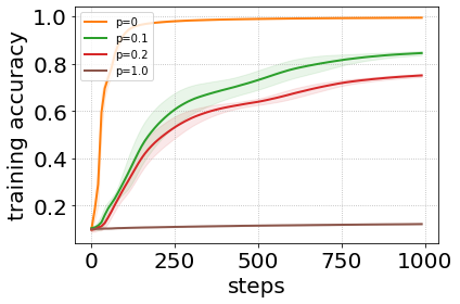
(a) training accuracy

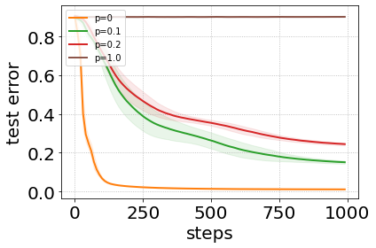
(b) test error

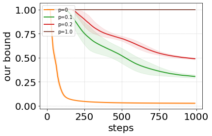
(c) our bound

Figure 3: Random labels (MNIST + FGD). Here $p$ is the portion of random labels.

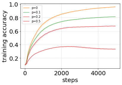
(a)

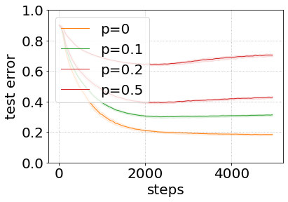
(b)

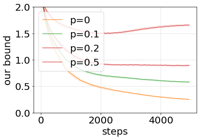
(c)

Figure 4: Random labels (FSGD + CIFAR10).

FGD vs GD

We attempt to show that the performance of FGD (Algorithm 1) with reasonable precision $\varepsilon_{t}$ is similar to the traditional Gradient Descent (GD) defined below (with momentum $\alpha$):

$$W_{t}\leftarrow W_{t-1}+\alpha(W_{t-1}-W_{t-2})+\gamma_{t}\nabla f(W_{t-1},S).$$ (GD)

We train a CNN defined above on MNIST by GD ($\gamma_{t}=0.005\times 0.9^{\lfloor\frac{t}{150}\rfloor}$, $\alpha=0.9$). And we compare the training curves with that of FGD under the same hyper-parameter setting ($\varepsilon_{t}=\gamma_{t}=0.005$, $\alpha=0.9$). We repeat our experiment on GD $25$ times. The result is shown in Figure 5.

(a) FGD

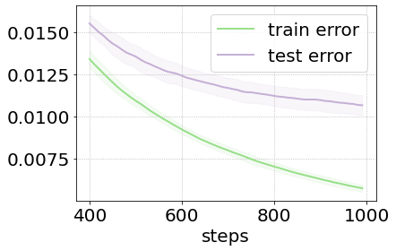
(b) GD

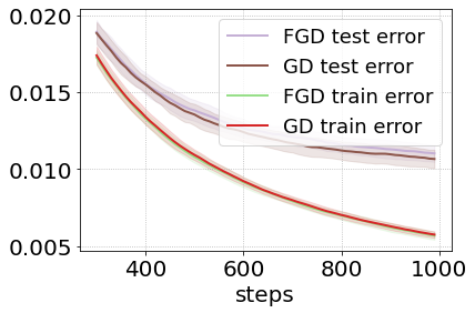
(c) together

Figure 5: MNIST: FGD vs GD. In (c), we plot FGD and GD together. As we can see that, the curves of FGD and GD are almost coincident.

(a) FSGD

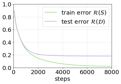
(b) SGD

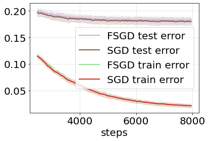
(c) together

Figure 6: CIFAR10: FSGD vs SGD.

As we can see from the figures, the optimization as well as generalization performance of GD and FGD are close.

FSGD vs SGD

We also show that the performance of FSGD (Algorithm 2) with reasonable precision $\varepsilon_{t}$ is very close to the ordinary Stochastic Gradient Descent (SGD) defined below (with momentum $\alpha$ and a). The only difference is that we sample a mini-batch $B_{t}$ before each step.:

$$W_{t}\leftarrow W_{t-1}+\alpha(W_{t-1}-W_{t-2})+\gamma_{t}\nabla f(W_{t-1},S_{B_{t}}).$$ (SGD)

We train a SimpleNet defined above on CIFAR10 by SGD ($\gamma_{t}=0.001$, $\alpha=0.99$). And we compare the training curves with that of FSGD under the same hyper-parameter setting ($\varepsilon_{t}=0.001,\gamma_{t}=0.001\times 0.9^{\lfloor\frac{t}{200}\rfloor},\alpha=0.99$). We repeat our experiment on SGD $10$ times. The result is shown in Figure 6. As we can see from the figures, the optimization as well as generalization performance of FSGD are close to SGD.

References

- Arora et al. [2018] Sanjeev Arora, Rong Ge, Behnam Neyshabur, and Yi Zhang. Stronger generalization bounds for deep nets via a compression approach. In International Conference on Machine Learning, pages 254–263. PMLR, 2018.
- Arora et al. [2019] Sanjeev Arora, Simon Du, Wei Hu, Zhiyuan Li, and Ruosong Wang. Fine-grained analysis of optimization and generalization for overparameterized two-layer neural networks. In International Conference on Machine Learning, pages 322–332. PMLR, 2019.
- Bartlett et al. [2017] Peter L Bartlett, Dylan J Foster, and Matus J Telgarsky. Spectrally-normalized margin bounds for neural networks. Advances in neural information processing systems, 30, 2017.
- Bousquet and Elisseeff [2002] Olivier Bousquet and André Elisseeff. Stability and generalization. The Journal of Machine Learning Research, 2:499–526, 2002.
- Bousquet et al. [2020] Olivier Bousquet, Yegor Klochkov, and Nikita Zhivotovskiy. Sharper bounds for uniformly stable algorithms. In Conference on Learning Theory, pages 610–626. PMLR, 2020.
- Bu et al. [2020] Yuheng Bu, Shaofeng Zou, and Venugopal V Veeravalli. Tightening mutual information-based bounds on generalization error. IEEE Journal on Selected Areas in Information Theory, 1(1):121–130, 2020.
- Cao and Gu [2019] Yuan Cao and Quanquan Gu. Generalization bounds of stochastic gradient descent for wide and deep neural networks. Advances in neural information processing systems, 32, 2019.
- Catoni [2007] Olivier Catoni. Pac-bayesian supervised classification: the thermodynamics of statistical learning. IMS Lecture Notes Monograph Series, 56:1–163, 2007. doi: 10.1214/074921707000000391.
- Chaudhari et al. [2019] Pratik Chaudhari, Anna Choromanska, Stefano Soatto, Yann LeCun, Carlo Baldassi, Christian Borgs, Jennifer Chayes, Levent Sagun, and Riccardo Zecchina. Entropy-sgd: Biasing gradient descent into wide valleys. Journal of Statistical Mechanics: Theory and Experiment, 2019(12):124018, 2019.
- Chen et al. [2020] Xi Chen, Simon S Du, and Xin T Tong. On stationary-point hitting time and ergodicity of stochastic gradient langevin dynamics. Journal of Machine Learning Research, 2020.
- Chen et al. [2018] Yuansi Chen, Chi Jin, and Bin Yu. Stability and convergence trade-off of iterative optimization algorithms. CoRR, 2018.
- Cover [1999] Thomas M Cover. Elements of information theory. John Wiley & Sons, 1999.
- Donsker and Varadhan [1983] Monroe D Donsker and SR Srinivasa Varadhan. Asymptotic evaluation of certain markov process expectations for large time. iv. Communications on pure and applied mathematics, 36(2):183–212, 1983.
- Du et al. [2019] Simon Du, Jason Lee, Haochuan Li, Liwei Wang, and Xiyu Zhai. Gradient descent finds global minima of deep neural networks. In International conference on machine learning, pages 1675–1685. PMLR, 2019.
- Dubhashi and Panconesi [2009] Devdatt P. Dubhashi and Alessandro Panconesi. Concentration of Measure for the Analysis of Randomized Algorithms. Cambridge University Press, 2009. ISBN 978-0-521-88427-3.
- Duchi [2007] John Duchi. Derivations for linear algebra and optimization. Berkeley, California, 3(1):2325–5870, 2007.
- Dziugaite and Roy [2017] Gintare Karolina Dziugaite and Daniel M Roy. Computing nonvacuous generalization bounds for deep (stochastic) neural networks with many more parameters than training data. UAI, 2017.
- Dziugaite et al. [2021] Gintare Karolina Dziugaite, Kyle Hsu, Waseem Gharbieh, Gabriel Arpino, and Daniel Roy. On the role of data in pac-bayes bounds. In International Conference on Artificial Intelligence and Statistics, pages 604–612. PMLR, 2021.
- Feldman and Vondrak [2019] Vitaly Feldman and Jan Vondrak. High probability generalization bounds for uniformly stable algorithms with nearly optimal rate. In Conference on Learning Theory, pages 1270–1279. PMLR, 2019.
- Golowich et al. [2018] Noah Golowich, Alexander Rakhlin, and Ohad Shamir. Size-independent sample complexity of neural networks. In Conference On Learning Theory, pages 297–299. PMLR, 2018.
- Haghifam et al. [2020] Mahdi Haghifam, Jeffrey Negrea, Ashish Khisti, Daniel M Roy, and Gintare Karolina Dziugaite. Sharpened generalization bounds based on conditional mutual information and an application to noisy, iterative algorithms. Advances in Neural Information Processing Systems, 33:9925–9935, 2020.
- Hardt et al. [2016] Moritz Hardt, Ben Recht, and Yoram Singer. Train faster, generalize better: Stability of stochastic gradient descent. In International conference on machine learning, pages 1225–1234. PMLR, 2016.
- Harvey et al. [2017] Nick Harvey, Christopher Liaw, and Abbas Mehrabian. Nearly-tight vc-dimension bounds for piecewise linear neural networks. In Conference on learning theory, pages 1064–1068. PMLR, 2017.
- Hasanpour et al. [2016] Seyyed Hossein Hasanpour, Mohammad Rouhani, Mohsen Fayyaz, and Mohammad Sabokrou. Lets keep it simple, using simple architectures to outperform deeper and more complex architectures. CoRR, 2016.
- Hodgkinson et al. [2022] Liam Hodgkinson, Umut Simsekli, Rajiv Khanna, and Michael Mahoney. Generalization bounds using lower tail exponents in stochastic optimizers. In International Conference on Machine Learning, pages 8774–8795. PMLR, 2022.
- Jacot et al. [2018] Arthur Jacot, Franck Gabriel, and Clément Hongler. Neural tangent kernel: Convergence and generalization in neural networks. Advances in neural information processing systems, 31, 2018.
- Krizhevsky et al. [2009] Alex Krizhevsky, Geoffrey Hinton, et al. Learning multiple layers of features from tiny images. Master’s thesis, University of Tront, 2009.
- Kuzborskij and Lampert [2018] Ilja Kuzborskij and Christoph Lampert. Data-dependent stability of stochastic gradient descent. In International Conference on Machine Learning, pages 2815–2824. PMLR, 2018.
- LeCun et al. [1998] Yann LeCun, Léon Bottou, Yoshua Bengio, and Patrick Haffner. Gradient-based learning applied to document recognition. Proceedings of the IEEE, 86(11):2278–2324, 1998.
- Lever et al. [2013] Guy Lever, François Laviolette, and John Shawe-Taylor. Tighter pac-bayes bounds through distribution-dependent priors. Theoretical Computer Science, 473:4–28, 2013.
- Li et al. [2020] Jian Li, Xuanyuan Luo, and Mingda Qiao. On generalization error bounds of noisy gradient methods for non-convex learning. In International Conference on Learning Representations, 2020.
- Li et al. [2017] Qianxiao Li, Cheng Tai, and E Weinan. Stochastic modified equations and adaptive stochastic gradient algorithms. In International Conference on Machine Learning, pages 2101–2110. PMLR, 2017.
- Li et al. [2021] Zhiyuan Li, Sadhika Malladi, and Sanjeev Arora. On the validity of modeling sgd with stochastic differential equations (sdes). Advances in Neural Information Processing Systems, 34, 2021.
- London [2016] Ben London. Generalization bounds for randomized learning with application to stochastic gradient descent. In NIPS Workshop on Optimizing the Optimizers, 2016.
- London [2017] Ben London. A pac-bayesian analysis of randomized learning with application to stochastic gradient descent. Advances in Neural Information Processing Systems, 30, 2017.
- McAllester [1999] David A McAllester. Some pac-bayesian theorems. Machine Learning, 37(3):355–363, 1999.
- Mou et al. [2018] Wenlong Mou, Liwei Wang, Xiyu Zhai, and Kai Zheng. Generalization bounds of sgld for non-convex learning: Two theoretical viewpoints. In Conference on Learning Theory, pages 605–638. PMLR, 2018.
- Nagarajan and Kolter [2017] Vaishnavh Nagarajan and J Zico Kolter. Generalization in deep networks: The role of distance from initialization. NeurIPS, 2017.
- Nagarajan and Kolter [2019] Vaishnavh Nagarajan and J Zico Kolter. Uniform convergence may be unable to explain generalization in deep learning. Advances in Neural Information Processing Systems, 32, 2019.
- Negrea et al. [2019] Jeffrey Negrea, Mahdi Haghifam, Gintare Karolina Dziugaite, Ashish Khisti, and Daniel M Roy. Information-theoretic generalization bounds for sgld via data-dependent estimates. Advances in Neural Information Processing Systems, 32, 2019.
- Neyshabur et al. [2018] Behnam Neyshabur, Srinadh Bhojanapalli, and Nathan Srebro. A pac-bayesian approach to spectrally-normalized margin bounds for neural networks. In International Conference on Learning Representations, 2018.
- Oneto et al. [2017] Luca Oneto, Sandro Ridella, and Davide Anguita. Differential privacy and generalization: Sharper bounds with applications. Pattern Recognition Letters, 89:31–38, 2017.
- Parrado-Hernández et al. [2012] Emilio Parrado-Hernández, Amiran Ambroladze, John Shawe-Taylor, and Shiliang Sun. Pac-bayes bounds with data dependent priors. The Journal of Machine Learning Research, 13(1):3507–3531, 2012.
- Pensia et al. [2018] Ankit Pensia, Varun Jog, and Po-Ling Loh. Generalization error bounds for noisy, iterative algorithms. In 2018 IEEE International Symposium on Information Theory (ISIT), pages 546–550. IEEE, 2018.
- Raginsky et al. [2017] Maxim Raginsky, Alexander Rakhlin, and Matus Telgarsky. Non-convex learning via stochastic gradient langevin dynamics: a nonasymptotic analysis. In Conference on Learning Theory, pages 1674–1703. PMLR, 2017.
- Risken [1996] Hannes Risken. Fokker-planck equation. In The Fokker-Planck Equation, pages 63–95. Springer, 1996.
- Simsekli et al. [2020] Umut Simsekli, Ozan Sener, George Deligiannidis, and Murat A Erdogdu. Hausdorff dimension, heavy tails, and generalization in neural networks. Advances in Neural Information Processing Systems, 33:5138–5151, 2020.
- Wang et al. [2021] Hao Wang, Yizhe Huang, Rui Gao, and Flavio Calmon. Analyzing the generalization capability of sgld using properties of gaussian channels. Advances in Neural Information Processing Systems, 34, 2021.
- Wei et al. [2019] Colin Wei, Jason D Lee, Qiang Liu, and Tengyu Ma. Regularization matters: Generalization and optimization of neural nets vs their induced kernel. Advances in Neural Information Processing Systems, 32, 2019.
- Welling and Teh [2011] Max Welling and Yee W Teh. Bayesian learning via stochastic gradient langevin dynamics. In Proceedings of the 28th international conference on machine learning (ICML-11), pages 681–688. Citeseer, 2011.
- Wu et al. [2021] Bingzhe Wu, Zhicong Liang, Yatao Bian, ChaoChao Chen, Junzhou Huang, and Yuan Yao. Generalization bounds for stochastic gradient langevin dynamics: A unified view via information leakage analysis. CoRR, 2021.
- Yang et al. [2019] Jun Yang, Shengyang Sun, and Daniel M Roy. Fast-rate pac-bayes generalization bounds via shifted rademacher processes. Advances in Neural Information Processing Systems, 32, 2019.
- Zantedeschi et al. [2021] Valentina Zantedeschi, Paul Viallard, Emilie Morvant, Rémi Emonet, Amaury Habrard, Pascal Germain, and Benjamin Guedj. Learning stochastic majority votes by minimizing a pac-bayes generalization bound. Advances in Neural Information Processing Systems, 34:455–467, 2021.
- Zhang et al. [2017] Chiyuan Zhang, Samy Bengio, Moritz Hardt, Benjamin Recht, and Oriol Vinyals. Understanding deep learning requires rethinking generalization. In 5th International Conference on Learning Representations, ICLR 2017, Toulon, France, April 24-26, 2017, Conference Track Proceedings. OpenReview.net, 2017.
- Zhang et al. [2017] Yuchen Zhang, Percy Liang, and Moses Charikar. A hitting time analysis of stochastic gradient langevin dynamics. In Conference on Learning Theory, pages 1980–2022. PMLR, 2017.
- Zhou et al. [2019] Wenda Zhou, Victor Veitch, Morgane Austern, Ryan P. Adams, and Peter Orbanz. Non-vacuous generalization bounds at the imagenet scale: a pac-bayesian compression approach. In 7th International Conference on Learning Representations, ICLR 2019, New Orleans, LA, USA, May 6-9, 2019. OpenReview.net, 2019.
- Zhu et al. [2019] Zhanxing Zhu, Jingfeng Wu, Bing Yu, Lei Wu, and Jinwen Ma. The anisotropic noise in stochastic gradient descent: Its behavior of escaping from sharp minima and regularization effects. In International Conference on Machine Learning, pages 7654–7663. PMLR, 2019.
- Ziyin et al. [2021] Liu Ziyin, Kangqiao Liu, Takashi Mori, and Masahito Ueda. Strength of minibatch noise in sgd. In International Conference on Learning Representations, 2021.