Improving Item Cold-start Recommendation via Model-agnostic Conditional Variational Autoencoder

Abstract.

Embedding & MLP has become a paradigm for modern large-scale recommendation system. However, this paradigm suffers from the cold-start problem which will seriously compromise the ecological health of recommendation systems. This paper attempts to tackle the item cold-start problem by generating enhanced warmed-up ID embeddings for cold items with historical data and limited interaction records. From the aspect of industrial practice, we mainly focus on the following three points of item cold-start: 1) How to conduct cold-start without additional data requirements and make strategy easy to be deployed in online recommendation scenarios. 2) How to leverage both historical records and constantly emerging interaction data of new items. 3) How to model the relationship between item ID and side information stably from interaction data. To address these problems, we propose a model-agnostic Conditional Variational Autoencoder based Recommendation() framework with some advantages including compatibility on various backbones, no extra requirements for data, utilization of both historical data and recent emerging interactions. uses latent variables to learn a distribution over item side information and generates desirable item ID embeddings using a conditional decoder. The proposed method is evaluated by extensive offline experiments on public datasets and online A/B tests on Tencent News recommendation platform, which further illustrate the advantages and robustness of .

1. Introduction

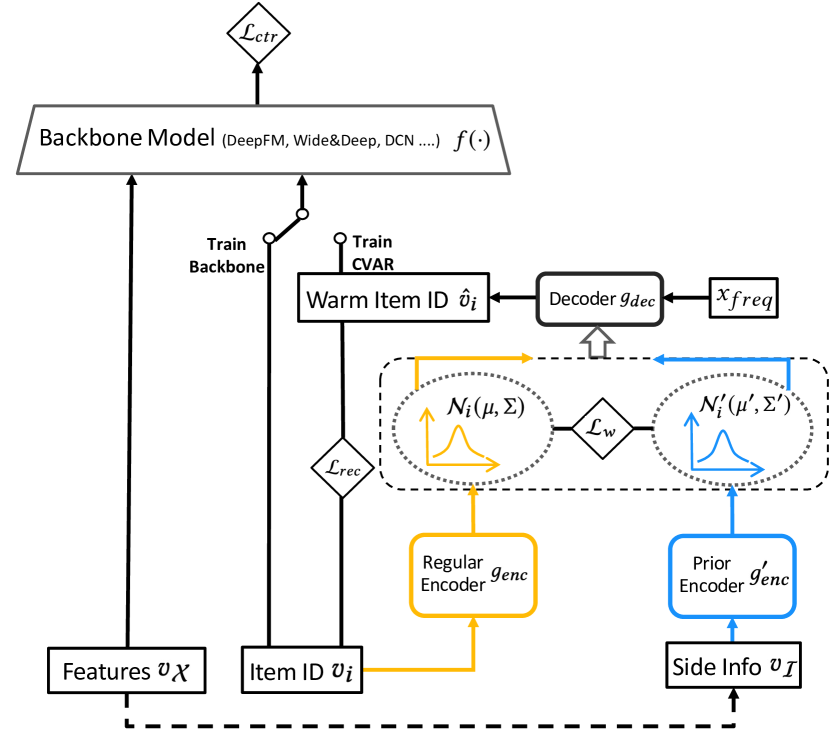
Figure 1. The proposed model-agnostic Framework, where Backbone Model can be any CTR prediction model with embedding layer.

In the era of mobile internet, various online applications continuously emerge and explosively grow, in which recommendation systems play a key role in connecting users and content. Due to the excellent scalability and convenience of handling massive features, Embedding & MLP (Sedhain et al., 2015; He and Chua, 2017; Guo et al., 2017; Cheng et al., 2016) has become a paradigm for modern large-scale recommendation systems (Zhou et al., 2018; Ma et al., 2018; Covington et al., 2016; Zhou et al., 2019; Davidson et al., 2010). However, this paradigm is data demanding and suffers from cold-start problem (Lam et al., 2008; Sethi and Mehrotra, 2021; Gope and Jain, 2017). Concretely, for a large amount of new emerging items with limited interactions, their embeddings are insufficiently trained which leads to poor recommendation performance. The cold-start problem has become a crucial obstacle for online recommendation. Under the influence of Pareto (Ribeiro et al., 2014) effect in our industrial system, A small portion of well-trained items tend to obtain more accurate recommendations and more impressions, which will further compromise the distributing efficiency of system.

Some approaches have been proposed to address the item cold-start challenge. CLCRec (Wei et al., 2021) proposes to address cold-start problem by maximizing two kinds of mutual information using contrastive learning technology. Heater (Zhu et al., 2020) uses the sum squared error (SSE) loss to model the collaborative embedding. Notice that CLCRec and Heater are only designed for the CF-based backbone models. There are also some model-agnostic methods that could be widely equipped to various backbones. DropoutNet (Volkovs et al., 2017) applies dropout technology to relieve the model‘s dependency on item ID. Meta Embedding (Pan et al., 2019) focuses on learning how to learn the ID embedding for new items with meta learning technology. MWUF (Zhu et al., 2021) proposes meta Scaling and meta Shifting Networks to warm up cold ID embeddings. Although these methods are model-agnostic, they all have extra and strict requirements on data. For instance, DropoutNet and MWUF require the interacted user set of items for cold-start, while Meta Embedding requires building two mini-batches containing the same items for training. In the online scenario of industrial recommendation, these extra requirements on data stream make the deployment process rather difficult.

Generally, there are two ways to solve the cold-start problem: the first is to mine the distribution patterns hidden in historical data (Zheng et al., 2021; Wang et al., 2020a; Pan et al., 2019; Zhu et al., 2021; Zhao et al., 2020a), such as learning the transformation relationship between side information and item ID (Wei et al., 2021; Zhu et al., 2020; Pan et al., 2019; Zhu et al., 2021). The second is to improve the learning efficiency with limited samples of cold items, such as methods based on meta learning (Lee et al., 2019; Zhang et al., 2021; Ouyang et al., 2021; Lu et al., 2020). However, previous works rarely consider both directions at the same time. In other words, methods in the first category only focus on the initialization of embedding, while the methods in the second category usually ignore patterns hidden in historical data.

Considering the issues mentioned above in previous research along with our industrial practice, we summarize three key points for the design of cold-start method: 1) How to conduct cold-start without additional data requirements and make strategy easy to be deployed in online recommendation scenario. 2) How the cold-start method can leverage both historical records and constantly emerging interaction data of new items. 3) How to model the relationship between item ID and side information stably from interaction data and minimize the discrepancy between cold item ID embedding and fully trained embedding space.

To achieve these desiderata, we propose a Conditional Variational Autoencoder based model-agnostic Recommendation () framework. As an independent framework, could be equipped on various backbone models and be trained in an end-to-end way, using the same samples as backbone. Thus makes no redundant requirements for training data. In addition to giving desirable initialization in the cold-start phase, will leverage the continuously updating item ID embeddings from the backbone to generate enhanced warmed-up embeddings with superior quality. Therefore can fulfill the second concern mentioned above.

As for the third problem mentioned before, aligns the representation of item ID and side information in the latent space of Conditional Variational AutoEncoder(CVAE) (Sohn et al., 2015; Zhao et al., 2017; Walker et al., 2016), which is shown in Figure 1. Specifically, previous works (Zhu et al., 2020; Pan et al., 2019; Zhu et al., 2021) usually train a learnable mapping from item side information to item ID. However, item ID contains not only content information, but also lots of interaction information which makes it difficult to learn a precise mapping directly. Inspired by Denoise Autoencoder (Vincent et al., 2010), we first conduct dimension reduction of item ID embedding with Encoder-Decoder paradigm and get the denoised representation of item ID in a latent space. Then the side information is transformed to the latent space and aligned with the denoised representation of item ID. Corresponding with the design in CVAE, latent representation is defined as normal distribution which could maintain some Exploit-Exposure ability for .

The main contributions of this work are summarized into four folds:

1. We propose a model-agnostic to warm up cold item ID embeddings. has no extra data requirements which makes it easy to be deployed in online scenario.

2. not only learns the pattern in historical data but also leverages the continuously updating item ID embedding from the backbone to generate enhanced warmed-up embeddings with superior quality.

3. We propose to model the relationship between item id and side information in the latent space and generate desirable ID embeddings using a conditional decoder.

4. Extensive offline and online experiments are conducted to demonstrate the effectiveness and compatibility of .

2. Proposed Method

In this section, we propose , a model-agnostic framework to warm up ID embeddings for new items. is designed based on the Click-Through-Rate(CTR) prediction task (Richardson et al., 2007; Graepel et al., 2010), predicting the click/watch/purchase behavior in recommendation scenario, which is usually formulated as a supervised binary classification task. Each sample in CTR task consists of multiple input features $\mathbf{x}$ and the binary label $y$. Generally, the input features x could be splitted into three parts, i.e. $\mathbf{x}=(i,\mathcal{X})$.

• $i$, item ID, a unique number or string to identify each item in recommendation system.

• $\mathcal{X}=\{x_{1},...,x_{|\mathcal{X}|}\}$, features which are used for CTR predict , may be categorical or continuous, such as the user attributes and contextual information.

Moreover, We take part of features from $\mathcal{X}$ as item side information $\mathcal{I}\subset\mathcal{X}$, which will be consumed in item cold-start procedure. Standard feature preprocessing (Richardson et al., 2007; Graepel et al., 2010) has been applied in this work. Continuous features are normalized to range between 0 and 1. Following the embedding technology (Le and Mikolov, 2014; Mikolov et al., 2013), categorical features are transformed to dense vectors, called embeddings. Normalized values of continuous features and dense embeddings of categorical features are concatenated together to constitute the final representation of input features. We denote the representations of $i$, $\mathcal{I}$, $\mathcal{X}$ as $v_{i}\in\mathbb{R}^{d}$, $v_{\mathcal{I}}\in\mathbb{R}^{d\times|\mathcal{I}|}$ and $v_{\mathcal{X}}\in\mathbb{R}^{d\times|\mathcal{X}|}$ respectively. Note that $v_{\mathcal{I}}$ and $v_{\mathcal{X}}$ are the concatenation of multiple feature embeddings.

The CTR target is to approximate the probability $\hat{y}=Pr(y=1|\mathbf{x})$ by a discriminative function $f(\cdot)$:

(1) $$\hat{y}=f(v_{i},v_{\mathcal{X}};\theta)$$

where $\theta$ denotes the parameters of the backbone model $f(\cdot)$. Then the Binary Cross Entropy (De Boer et al., 2005) is used to format the loss function:

(2) $$\mathcal{L}(\theta,\phi)=-y\log\hat{y}-(1-y)\log(1-\hat{y})$$

where $\phi$ denotes the parameters of the embedding layer, including $v_{i}$, $v_{\mathcal{I}}$ and $v_{\mathcal{X}}$. As the parameters is trained by historical data, the item ID embeddings of recent emerging items are rarely updated and stay around the initial point, leading to a low testing accuracy. It is known as the item cold-start problem.

As the relationship between cold-start and warm-up in recommendation system is confusing, we will give a brief discussion here. Generally speaking, cold-start strategies are applied to items which first appear in the system, while warm-up strategies are applied to items whose exposure numbers are lower than a threshold. Note that this threshold is inconsistent across different systems. In other words, warm-up is a subsequent procedure of cold-start. In this work, We conduct cold-start and warm-up in a unified framework .

The structure of is shown in Figure 1. The basic design of is generating a better embedding for item ID and replace the original unsufficiently trained embedding. The Item ID in Figure 1 denotes the original item ID embedding $v_{i}$ trained by backbone model, while the Warm Item ID denotes the enhanced warmed-up embedding $\hat{v}_{i}$ generated by . Instead of directly learning a transformation from $v_{\mathcal{I}}$ to $v_{i}$, aligns the representations transformed from $v_{i}$ and $v_{\mathcal{I}}$ in the autoencoder’s latent space (Wang et al., 2016; Durkan et al., 2019; Ye et al., 2021). Following the design of CVAE (Sohn et al., 2015), the autoencoder applied to $v_{i}$ is formulated as:

(3) $$\mu,\sigma=g_{enc}(v_{i};w_{enc});\mu\in\mathbb{R}^{k},\sigma\in\mathbb{R}^{k}$$

(4) $$z\sim\mathcal{N}_{i}(\mu,\Sigma);\Sigma\in\mathbb{R}^{k\times k},diag(\Sigma)=\sigma$$

(5) $$\hat{v}_{i}=g_{dec}(z,x_{freq};w_{dec});\hat{v}_{i}\in\mathbb{R}^{d}$$

where $g_{enc}$ and $g_{dec}$ correspond to the Regular Encoder and Decoder in Figure 1, $w_{enc}$ and $w_{dec}$ denote the parameters of $g_{enc}$ and $g_{dec}$, $k$ denotes the dimension of latent space. Notice that as shown in Equation (3) the latent representation is defined as a multivariate normal distribution $\mathcal{N}_{i}(\mu,\Sigma)$ with mean $\mu$ and diagonal covariance matrix $\Sigma$ whose trace is $\sigma$. In Equation (4), latent representation $z$ is sampled from $\mathcal{N}_{i}(\mu,\Sigma)$ using the reparameterization trick (Pham and Le, 2020). Decoder $g_{dec}$ takes $z$ along with conditional frequency $x_{freq}$ as input and reconstructs item ID embedding as $\hat{v}_{i}$. Since the item frequency information has a direct impact on the distribution of ID embedding and is operated in the entire warm-up phase, unlike traditional CVAE design (Sohn et al., 2015; Zhao et al., 2017; Walker et al., 2016), we only filter $x_{freq}$ from the full side information as the condition of decoder to emphasize its impact.

Reconstruction Loss between $v_{i}$ and $\hat{v}_{i}$ is formulated by Euclidean distance:

(6) $$\mathcal{L}_{rec}(w_{enc},w_{dec})=\|v_{i}-\hat{v}_{i}\|^{2}_{2}$$

Notice that rarely updated $v_{i}$ of almost cold items in Equation (6) may mislead the training procedure. However, with $x_{freq}$ as condition to $g_{dec}$, the generated embedding will be restricted to a reasonable space according to $x_{freq}$ which could relieve this misleading effect. Thus we do not deal with this case separately. Besides, in inference stage, we set $x_{freq}$ as a huge value which will help to produce warm ID embeddings.

Through the autoencoder structure described above, we obtain the information-compressed latent distribution $\mathcal{N}_{i}(\mu,\Sigma)$ of $v_{i}$. Aligning embeddings or distributions in autoencoder’s latent space is a generally used technology which has been proven effective in various fields (Durkan et al., 2019). Thus we consider mapping the side information embedding $v_{\mathcal{I}}$ into the same latent space and aligning with $\mathcal{N}_{i}(\mu,\Sigma)$. Specifically, Prior Encoder $g^{\prime}_{enc}$ maps $v_{\mathcal{I}}$ to $\mathcal{N}_{i}(\mu^{\prime},\Sigma^{\prime})$ and a wasserstein loss (Peyré et al., 2019; Shen et al., 2018) function is applied to aligning distribution $\mathcal{N}_{i}(\mu,\Sigma)$ with $\mathcal{N}_{i}(\mu^{\prime},\Sigma^{\prime})$:

(7) $$\mu^{\prime},\sigma^{\prime}=g^{\prime}_{enc}(v_{\mathcal{I}};w^{\prime}_{enc});\mu^{\prime}\in\mathbb{R}^{k},\sigma^{\prime}\in\mathbb{R}^{k}$$

(8) $$z^{\prime}\sim\mathcal{N}_{i}^{\prime}(\mu^{\prime},\Sigma^{\prime});\Sigma^{\prime}\in\mathbb{R}^{k\times k},trace(\Sigma^{\prime})=\sigma^{\prime}$$

(9) $$\hat{v}_{i}^{\prime}=g_{dec}(z^{\prime},x_{freq};w_{dec});\hat{v}_{i}^{\prime}\in\mathbb{R}^{d}$$

(10) $$\mathcal{L}_{w}(w_{enc},w^{\prime}_{enc})=W_{2}(\mathcal{N}_{i}(\mu,\Sigma),\mathcal{N}_{i}^{\prime}(\mu^{\prime},\Sigma^{\prime}))$$

where $w^{\prime}_{enc}$ denotes the parameters of $g^{\prime}_{enc}$, $W_{2}(\cdot,\cdot)$ denotes the Wasserstein Distance. Instead of KL Divergence (Bu et al., 2018) or other distribution measurement, we choose Wasserstein Distance considering its symmetry and stability which is widely used in various scenarios (Zhao et al., 2020b, c; Wang et al., 2020b; Liao et al., 2022).

We will give an additional discussion about the design of $x_{freq}$. Since that it’s not feasible to extract frequency information from side information by $g^{\prime}_{enc}$ in item cold start scenario, the latent space ideally should contain no frequency information. However, the frequency information is already utilized in the origin item ID embedding $v_{i}$ and automatically compressed to the latent space under the Encoder-Decoder framework. Thus we set $x_{freq}$ as the a independent condition of decoder to reduce the proportion of frequency information in latent space.

In addition to $\mathcal{L}_{rec}$ and $\mathcal{L}_{w}$, we replace $v_{i}$ in Equation (1) with enhanced warmed-up $\hat{v}_{i}^{\prime}$ as item ID input to backbone and get the CTR loss $\mathcal{L}_{ctr}$ by forward computation:

(11) $$\hat{y}_{warm} =f(\hat{v}_{i}^{\prime},v_{\mathcal{X}};\theta)$$

(12) $$\mathcal{L}_{ctr}(w_{enc},w_{dec})=-y\log \hat{y}_{warm}-(1-y)\log(1-\hat{y}_{warm})$$

To avoid disturbing the recommendation of hot items, is taken as an independent module with backbone. During the training of , optimization of $\mathcal{L}_{ctr}$ in Equation (12) is only applied to $w_{enc}$ and $w_{dec}$, while the parameters $\theta$ of $f(\cdot)$ are fixed. We finally get the loss function to train :

(13) $$\mathcal{L}_{warm}(w_{enc},w_{dec},w^{\prime}_{enc})=\mathcal{L}_{ctr}+\alpha\mathcal{L}_{rec}+\beta\mathcal{L}_{w}$$

where $\alpha$ and $\beta$ are hyperparameters to fuse the losses. Moreover, training of is along with the backbone’s training. As shown in Equation (13), will be trained by optimizing $w_{enc},w_{dec},w^{\prime}_{enc}$ to minimize $\mathcal{L}_{warm}$, using the same samples as training backbone, without any additional requirements on data. For a coming batch of samples, it’s first fed to backbone to update the original item ID embedding $v_{i}$, then used to train and update $w_{enc},w_{dec},w^{\prime}_{enc}$. Updated $v_{i}$ is also consumed in the training of at each step. Thus we claim that not only learns the pattern in historical data but also uses the information of update at each step to relieve the cold-start issue.

In inference phase of recent emerging items, their item ID embeddings $v_{i}$ are not well tained. Therefore we obtain $z{\prime}$ by sampling from $\mathcal{N}^{\prime}_{i}$ which is generated by item side information and get enhanced warmed-up ID item $\hat{v}_{i}^{\prime}$ by passing $z^{\prime}$ to $g_{dec}$ as Equation (7) and  (8) shown. Then we could replace $v_{i}$ with $v_{i}^{\prime}$ for testing of recent emerging items. As marked in Figure 1, Equation (4) and (5) are operated in training of , while Equation (8) and (9) play a role for recent emerging items in testing phase. For a single item, besides just searching for a better initialization of ID embedding, this replacement operation will continue until $v_{i}$ is fully trained.

3. Experiments

Table 1. Model Comparison of cold-start effectiveness on two datasets(Movielens 1M and Taobao Ad), under two backbones(DeepFM and Wide&Deep), three runs for each. The best improvements are highlighted in bold.

Methods	Cold phase		Warm-a phase		Warm-b phase		Warm-c phase
	AUC	F1	AUC	F1	AUC	F1	AUC	F1
Dataset: Movielens 1M & Backbone: DeepFM
DeepFM	0.7267	0.6231	0.7424	0.6383	0.7574	0.6503	0.7694	0.6608
DropoutNet	0.7387	0.6339	0.7491	0.6441	0.7587	0.6531	0.7673	0.6599
Meta-E	0.7327	0.6344	0.7441	0.6432	0.7544	0.6519	0.7633	0.6592
MWUF	0.7316	0.6289	0.7462	0.6413	0.7589	0.6521	0.7701	0.6616
1-9[1.5pt/2pt] (Init Only)	0.7401	0.6353	0.7518	0.6454	0.7624	0.6547	0.7717	0.6622
	0.7419	0.6356	0.7927	0.6789	0.8021	0.6856	0.8041	0.6878
Dataset: Movielens 1M & Backbone: Wide&Deep
Wide&Deep	0.7071	0.5972	0.7232	0.6164	0.7354	0.6273	0.7461	0.6372
DropoutNet	0.7125	0.6038	0.7228	0.6159	0.7313	0.6244	0.7390	0.6314
Meta-E	0.6727	0.5287	0.7201	0.6120	0.7345	0.6280	0.7450	0.6374
MWUF	0.7063	0.5966	0.7230	0.6157	0.7355	0.6275	0.7459	0.6366
1-9[1.5pt/2pt] (Init Only)	0.7020	0.5795	0.7255	0.6160	0.7375	0.6293	0.7473	0.6380
	0.6937	0.5643	0.7627	0.6525	0.7756	0.6639	0.7840	0.6712
Dataset: Taobao Ad & Backbone: DeepFM
DeepFM	0.5983	0.1350	0.6097	0.1378	0.6207	0.1401	0.6311	0.1438
DropoutNet	0.5989	0.1352	0.6098	0.1374	0.6203	0.1396	0.6302	0.1435
Meta-E	0.5982	0.1346	0.6093	0.1377	0.6195	0.1400	0.6294	0.1428
MWUF	0.5986	0.1348	0.6082	0.1374	0.6184	0.1399	0.6279	0.1429
1-9[1.5pt/2pt] (Init Only)	0.5987	0.1350	0.6098	0.1376	0.6204	0.1398	0.6306	0.1432
	0.5978	0.1347	0.6198	0.1408	0.6308	0.1477	0.6380	0.1503
Dataset: Taobao Ad & Backbone: Wide&Deep
Wide&Deep	0.6081	0.1360	0.6129	0.1427	0.6207	0.1455	0.6287	0.1484
DropoutNet	0.6095	0.1359	0.6184	0.1427	0.6246	0.1454	0.6312	0.1474
Meta-E	0.6082	0.1378	0.6122	0.1443	0.6190	0.1477	0.6259	0.1506
MWUF	0.6089	0.1382	0.6125	0.1423	0.6210	0.1457	0.6285	0.1483
1-9[1.5pt/2pt] (Init Only)	0.6027	0.1359	0.6065	0.1429	0.6163	0.1471	0.6232	0.1496
	0.6051	0.1368	0.6220	0.1457	0.6290	0.1495	0.6336	0.1511

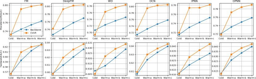
Figure 2. AUC curves through warming-up on two datasets, over six popular backbone models, three runs for each.

3.1. Offline Experiments

3.1.1. Experiment Setup

In this section, we will introduce the offline experiment setup.

Public Datasets. For offline experiments, We evaluate on the following two public datasets MovieLens-1M and Taobao Ad.

• MovieLens-1M: One of the most well-known recommendation benchmark dataset. The data consists of 1 million movie ranking instances over thousands of movies and users. Features of a movie include its title, year of release, and genres which are seen as item side information. Titles and genres are lists of tokens. Each user has features including the user’s ID, age, gender and occupation.

• Taobao Display Ad Click: It randomly samples 1140000 users from 26 million ad display / click records on Taobao  website to construct the dataset. We take each Ad as a item for CTR prediction, with 4 categorical attributes as side information, including category ID, campaign ID, brand ID, advertiser ID. Each user has features including Micro group ID, cms_group_id, gender, age, consumption grade, shopping depth, occupation and city level.

Dataset Split. To demonstrate the recommendation performance in both cold-start and warm-up phases, we conduct the experiments by splitting the datasets following (Pan et al., 2019) and (Zhu et al., 2021). We divide items into two groups, old and new based on their frequency, where items with more than $N$ labeled instances are old and others are new. We use $N$ of 200 and 2000 for Movielens-1M and Taobao Ad data. Note that the ratio of new items to old items is approximately 8:2, which is similar to the definition of long-tail items (Chen et al., 2020). Besides, new item instances sorted by timestamp are divided into four groups denoted as warm-a, -b, -c, and test set following (Pan et al., 2019) and (Zhu et al., 2021).

Backbones and Baselines. Because is model-agnostic, it can be applied to various existing models in the Embedding & MLP paradigm. Thus we conduct experiments upon the following representative backbones: FM (Rendle, 2010), DeepFM (Guo et al., 2017), Wide&Deep (Cheng et al., 2016), DCN (Wang et al., 2017), IPNN (Qu et al., 2016), OPNN (Qu et al., 2016). Meanwhile we choose some State-Of-The-Art(SOTA) methods for the item cold-start problem as baselines: DropoutNet (Volkovs et al., 2017), Meta embedding(Meta-E) (Pan et al., 2019), MWUF (Zhu et al., 2021). We reproduce each baseline based on open source code or their publications if the code is unavailable. We open all of the related source code on Github .

Implementation Details. For a fair comparison, we use the same setting for all methods. The MLPs in backbones and cold-start modules use the same structure with two dense layers (hidden units 16). The embedding size of each feature is fixed to 16. Learning rate and mini-batch size are set to 0.001 and 2048 respectively. At the inference stage, $x_{freq}$ of new emerging items is set to the largest item frequency in the corresponding dataset to generate warmed-up embeddings. Training is done with Adam (Kingma and Ba, 2015) optimizer over shuffled samples. In experiments, we firstly use old item instances to pretrain the backbone model as well as the cold-start module and evaluate on the test set(Initialization phase). Then we in turn feed warm-a, -b, -c data to train the backbone or and evaluate models on the test set step by step. We take the AUC score (Ling et al., 2003) and the F1 score (Huang et al., 2015) as evaluation metrics.

Table 2. performance(AUC) with different $x_{freq}$ on Movielens1M and Wide&Deep, three runs for each. The best improvements are highlighted in bold.

$x_{freq}$	Cold	Warm-a	Warm-b	Warm-c
0.01	0.6936	0.7627	0.7756	0.7839
0.1	0.6939	0.7629	0.7756	0.7837
0.25	0.6946	0.7627	0.7754	0.7842
0.5	0.6956	0.7638	0.7754	0.7844
1.0	0.6973	0.7649	0.7757	0.7845

3.1.2. Experimental Results

We compare the cold-start effectiveness of with backbone and three SOTA cold-start baselines including DropoutNet, Meta-E, MWUF. Meanwhile, we choose two most famous CTR prediction methods as backbones, DeepFM and Wide&Deep. To evaluate the quality of initial embedding generated by and further prove the effectiveness of in leveraging the changing id embedding for better warm-up, we conduct a version of contrast experiment for denoted as (Init Only), where only plays a role in initialization phase and is disabled in following three warm-up phases. We conduct experiments on two datasets and evaluate the mean results over three runs.

The main experimental results are shown in Table 1. Notice that (Init Only) outperforms other baselines in most cases, which indicates a high quality of initial embeddings generated by . Moreover, superior performance of (Init Only) proves that distribution alignment in latent space is better than directly mapping side information to item id which is adopted in Meta-E and MWUF. Except for a better initialization, can significantly improve the prediction performance in warm-up stages which is proven by the outstanding results of in Table 1. This phenomenon demonstrates that can indeed produce high quality warmed-up embedding based on the evolving item ID embedding learned by backbone in warm-up stage.

Method compatibility. Since is model-agnostic, we conduct experiments in more scenarios to verify its compatibility. Results on six popular backbones and two datasets in Figure 2 demonstrate the compatibility and robustness of .

Comparison of different frequency condition As mentioned before, $x_{freq}$ is set as the condition of decoder in and has a direct impact on the distribution of ID embedding. Considering the final $x_{freq}$ is uncertain for new emerging items at inference stage, we compare the performance of with different $x_{freq}$. Because $x_{freq}$ is normalized before using, we conduct five experiments with $x_{freq}$ equal 0.01, 0.1, 0.25, 0.5 and 1. Experimental results are shown in Table 2. It’s shown that performance of increases gradually with the increase of $x_{freq}$, which explains why we set $x_{freq}$ as a huge value at inference stage for cold start.

3.2. Online A/B tests

To verify the effectiveness of , we further conduct online A/B tests (Kohavi and Longbotham, 2017) for 7 days on Tencent News recommendation platform. As usually adopted in industry recommendation, the whole coarse-to-fine recommendation progress can be divided into four stages : candidate generation, coarse-grained ranking, fine-grained ranking, and re-ranking. In our industrial scenario, is applied to the ranking stage whose backbone is MMOE (Ma et al., 2018; Tang et al., 2020). Consistent with the four phases in offline experiments, we group online items into four groups: cold, warm-a, -b, -c, with increasing exposed frequency. In our system, there are two mediums of news: Article and Video. We focus on the following metrics (Gunawardana and Shani, 2009) (from high importance to low): Exposure Rate, Watch Time, Page(Video) Views. Exposure Rate measures the distribution percentage of the item group. Watch Time and Page(Video) Views reflect how users are attracted by recommended content.

We show the online results on various item groups in Table 3. It’s apparent that metrics of cold items are significantly improved, which proves the effectiveness of . As expected, the gain of gradually diminishes as the exposed frequency increases. Moreover, exposed items’ Gini coefficient (Zhou et al., 2010) on various item categories reduces from 0.7413 to 0.7369 after applying , which indicates could alleviate the Matthew Effect (Wang et al., 2018) to some extent.

Table 3. Online A/B results of item groups with increasing warm-up level: cold, warm-a, warm-b and warm-c. Red results mean they are statistically significant (whose p-value in hypothesis testing (Biau et al., 2010) is stable less than 0.05.)

Metrics	Cold	Warm-a	Warm-b	Warm-c	Total
Exposure Rate	+1.48%	-0.21%	-0.04%	+0.17%	-
Watch Time	+2.49%	+2.90%	+1.40%	+0.39%	+0.38%
Article Watch Time	+2.39%	+4.51%	+2.08%	+0.16%	+0.13%
Video Watch Time	+2.60%	+1.78%	+0.72%	+0.68%	+0.66%
Total Page Views	+4.46%	+2.87%	+1.42%	+0.62%	+1.09%
Article Page Views	+3.58%	+3.37%	+1.74%	+0.31%	+0.82%
Video Views	+5.84%	+2.25%	+1.05%	+1.01%	+1.35%

4. Conclusion

In this paper, we proposed the model-agnostic for item cold-start which uses latent variables to learn a distribution over side information and generates desirable ID embeddings using a conditional decoder. For better cold-start performance, not only learns the pattern in historical data but also leverages the continuously updating item ID embedding from the backbone to generate enhanced warmed-up embeddings with superior quality. From the aspect of industrial practice, we claim that additional strict data requirements of cold-start methods will make the deployment process rather difficult in online scenario. Thus is designed to be trained with the same raw samples as training main prediction model. Note that the proposed is a general framework that can be applied to various backbones. Finally, extensive offline experiments on public datasets and online A/B tests show the effectiveness and compatibility of .

References

- (1)
- Biau et al. (2010) David Jean Biau, Brigitte M Jolles, and Raphaël Porcher. 2010. P value and the theory of hypothesis testing: an explanation for new researchers. Clinical Orthopaedics and Related Research® 468, 3 (2010), 885–892.
- Bu et al. (2018) Yuheng Bu, Shaofeng Zou, Yingbin Liang, and Venugopal V Veeravalli. 2018. Estimation of KL divergence: Optimal minimax rate. IEEE Transactions on Information Theory 64, 4 (2018), 2648–2674.
- Chen et al. (2020) Zhihong Chen, Rong Xiao, Chenliang Li, Gangfeng Ye, Haochuan Sun, and Hongbo Deng. 2020. ESAM: Discriminative domain adaptation with non-displayed items to improve long-tail performance. In SIGIR.
- Cheng et al. (2016) Heng-Tze Cheng, Levent Koc, Jeremiah Harmsen, Tal Shaked, Tushar Chandra, Hrishi Aradhye, Glen Anderson, Greg Corrado, Wei Chai, Mustafa Ispir, et al. 2016. Wide & deep learning for recommender systems. In Recsys workshop.
- Covington et al. (2016) Paul Covington, Jay Adams, and Emre Sargin. 2016. Deep neural networks for youtube recommendations. In Recsys.
- Davidson et al. (2010) James Davidson, Benjamin Liebald, Junning Liu, Palash Nandy, Taylor Van Vleet, Ullas Gargi, Sujoy Gupta, Yu He, Mike Lambert, Blake Livingston, et al. 2010. The YouTube video recommendation system. In Recsys.
- De Boer et al. (2005) Pieter-Tjerk De Boer, Dirk P Kroese, Shie Mannor, and Reuven Y Rubinstein. 2005. A tutorial on the cross-entropy method. Annals of operations research 134, 1 (2005), 19–67.
- Durkan et al. (2019) Conor Durkan, Artur Bekasov, Iain Murray, and George Papamakarios. 2019. Neural spline flows. In NeurIPS.
- Gope and Jain (2017) Jyotirmoy Gope and Sanjay Kumar Jain. 2017. A survey on solving cold start problem in recommender systems. In ICCCA.
- Graepel et al. (2010) Thore Graepel, Joaquin Quinonero Candela, Thomas Borchert, and Ralf Herbrich. 2010. Web-scale bayesian click-through rate prediction for sponsored search advertising in microsoft’s bing search engine. In ICML.
- Gunawardana and Shani (2009) Asela Gunawardana and Guy Shani. 2009. A survey of accuracy evaluation metrics of recommendation tasks. Journal of Machine Learning Research 10, 12 (2009).
- Guo et al. (2017) Huifeng Guo, Ruiming Tang, Yunming Ye, Zhenguo Li, and Xiuqiang He. 2017. DeepFM: a factorization-machine based neural network for CTR prediction. In AAAI.
- He and Chua (2017) Xiangnan He and Tat-Seng Chua. 2017. Neural factorization machines for sparse predictive analytics. In SIGIR.
- Huang et al. (2015) Hao Huang, Haihua Xu, Xianhui Wang, and Wushour Silamu. 2015. Maximum F1-score discriminative training criterion for automatic mispronunciation detection. IEEE/ACM Transactions on Audio, Speech, and Language Processing 23, 4 (2015), 787–797.
- Kingma and Ba (2015) Diederik P Kingma and Jimmy Ba. 2015. Adam: A method for stochastic optimization. In ICLR.
- Kohavi and Longbotham (2017) Ron Kohavi and Roger Longbotham. 2017. Online Controlled Experiments and A/B Testing. Encyclopedia of machine learning and data mining 7, 8 (2017), 922–929.
- Lam et al. (2008) Xuan Nhat Lam, Thuc Vu, Trong Duc Le, and Anh Duc Duong. 2008. Addressing cold-start problem in recommendation systems. In ICUIMC. 208–211.
- Le and Mikolov (2014) Quoc V. Le and Tomás Mikolov. 2014. Distributed Representations of Sentences and Documents. In ICML.
- Lee et al. (2019) Hoyeop Lee, Jinbae Im, Seongwon Jang, Hyunsouk Cho, and Sehee Chung. 2019. Melu: Meta-learned user preference estimator for cold-start recommendation. In SIGKDD.
- Liao et al. (2022) Qichen Liao, Jing Chen, Zihao Wang, Bo Bai, Shi Jin, and Hao Wu. 2022. Fast Sinkhorn I: An O (N) algorithm for the Wasserstein-1 metric. arXiv preprint arXiv:2202.10042 (2022).
- Ling et al. (2003) Charles X Ling, Jin Huang, Harry Zhang, et al. 2003. AUC: a statistically consistent and more discriminating measure than accuracy. In IJCAI.
- Lu et al. (2020) Yuanfu Lu, Yuan Fang, and Chuan Shi. 2020. Meta-learning on heterogeneous information networks for cold-start recommendation. In SIGKDD.
- Ma et al. (2018) Jiaqi Ma, Zhe Zhao, Xinyang Yi, Jilin Chen, Lichan Hong, and Ed H Chi. 2018. Modeling task relationships in multi-task learning with multi-gate mixture-of-experts. In SIGKDD.
- Mikolov et al. (2013) Tomás Mikolov, Kai Chen, Greg Corrado, and Jeffrey Dean. 2013. Efficient Estimation of Word Representations in Vector Space. In ICLR.
- Ouyang et al. (2021) Wentao Ouyang, Xiuwu Zhang, Shukui Ren, Li Li, Kun Zhang, Jinmei Luo, Zhaojie Liu, and Yanlong Du. 2021. Learning graph meta embeddings for cold-start ads in click-through rate prediction. In SIGIR.
- Pan et al. (2019) Feiyang Pan, Shuokai Li, Xiang Ao, Pingzhong Tang, and Qing He. 2019. Warm up cold-start advertisements: Improving ctr predictions via learning to learn id embeddings. In SIGIR.
- Peyré et al. (2019) Gabriel Peyré, Marco Cuturi, et al. 2019. Computational optimal transport: With applications to data science. Foundations and Trends® in Machine Learning 11, 5-6 (2019), 355–607.
- Pham and Le (2020) Dang Pham and Tuan M. V. Le. 2020. Auto-Encoding Variational Bayes for Inferring Topics and Visualization. In COLING.
- Qu et al. (2016) Yanru Qu, Han Cai, Kan Ren, Weinan Zhang, Yong Yu, Ying Wen, and Jun Wang. 2016. Product-based neural networks for user response prediction. In ICDM.
- Rendle (2010) Steffen Rendle. 2010. Factorization machines. In ICDM.
- Ribeiro et al. (2014) Marco Tulio Ribeiro, Nivio Ziviani, Edleno Silva De Moura, Itamar Hata, Anisio Lacerda, and Adriano Veloso. 2014. Multiobjective pareto-efficient approaches for recommender systems. ACM Transactions on Intelligent Systems and Technology (TIST) 5, 4 (2014), 1–20.
- Richardson et al. (2007) Matthew Richardson, Ewa Dominowska, and Robert Ragno. 2007. Predicting clicks: estimating the click-through rate for new ads. In WWW.
- Sedhain et al. (2015) Suvash Sedhain, Aditya Krishna Menon, Scott Sanner, and Lexing Xie. 2015. Autorec: Autoencoders meet collaborative filtering. In WWW.
- Sethi and Mehrotra (2021) Rachna Sethi and Monica Mehrotra. 2021. Cold Start in Recommender Systems—A Survey from Domain Perspective. (2021), 223–232.
- Shen et al. (2018) Jian Shen, Yanru Qu, Weinan Zhang, and Yong Yu. 2018. Wasserstein distance guided representation learning for domain adaptation. In AAAI.
- Sohn et al. (2015) Kihyuk Sohn, Honglak Lee, and Xinchen Yan. 2015. Learning Structured Output Representation using Deep Conditional Generative Models. In NeurPIS.
- Tang et al. (2020) Hongyan Tang, Junning Liu, Ming Zhao, and Xudong Gong. 2020. Progressive layered extraction (ple): A novel multi-task learning (mtl) model for personalized recommendations. In Recsys.
- Vincent et al. (2010) Pascal Vincent, Hugo Larochelle, Isabelle Lajoie, Yoshua Bengio, Pierre-Antoine Manzagol, and Léon Bottou. 2010. Stacked denoising autoencoders: Learning useful representations in a deep network with a local denoising criterion. Journal of machine learning research (2010).
- Volkovs et al. (2017) Maksims Volkovs, Guangwei Yu, and Tomi Poutanen. 2017. Dropoutnet: Addressing cold start in recommender systems. In NeurIPS.
- Walker et al. (2016) Jacob Walker, Carl Doersch, Abhinav Gupta, and Martial Hebert. 2016. An uncertain future: Forecasting from static images using variational autoencoders. In ECCV.
- Wang et al. (2018) Hao Wang, Zonghu Wang, and Weishi Zhang. 2018. Quantitative analysis of Matthew effect and sparsity problem of recommender systems. In ICCCBDA.
- Wang et al. (2017) Ruoxi Wang, Bin Fu, Gang Fu, and Mingliang Wang. 2017. Deep & cross network for ad click predictions. In ADKDD.
- Wang et al. (2020a) Yifan Wang, Suyao Tang, Yuntong Lei, Weiping Song, Sheng Wang, and Ming Zhang. 2020a. Disenhan: Disentangled heterogeneous graph attention network for recommendation. In CIKM.
- Wang et al. (2016) Yasi Wang, Hongxun Yao, and Sicheng Zhao. 2016. Auto-encoder based dimensionality reduction. Neurocomputing 184 (2016), 232–242.
- Wang et al. (2020b) Zihao Wang, Datong Zhou, Ming Yang, Yong Zhang, Chenglong Rao, and Hao Wu. 2020b. Robust document distance with wasserstein-fisher-rao metric. In ACML.
- Wei et al. (2021) Yinwei Wei, Xiang Wang, Qi Li, Liqiang Nie, Yan Li, Xuanping Li, and Tat-Seng Chua. 2021. Contrastive learning for cold-start recommendation. In ACMMM.
- Ye et al. (2021) Wenhao Ye, Boxiang Ren, Zihao Wang, Huihui Wu, Hao Wu, Bo Bai, and Gong Zhang. 2021. Autoencoder-based MIMO Communications with Learnable ADCs. In ICCT.
- Zhang et al. (2021) Yin Zhang, Derek Zhiyuan Cheng, Tiansheng Yao, Xinyang Yi, Lichan Hong, and Ed H Chi. 2021. A model of two tales: Dual transfer learning framework for improved long-tail item recommendation. In WWW.
- Zhao et al. (2020a) Cheng Zhao, Chenliang Li, Rong Xiao, Hongbo Deng, and Aixin Sun. 2020a. CATN: Cross-domain recommendation for cold-start users via aspect transfer network. In SIGIR.
- Zhao et al. (2017) Tiancheng Zhao, Ran Zhao, and Maxine Eskénazi. 2017. Learning Discourse-level Diversity for Neural Dialog Models using Conditional Variational Autoencoders. In ACL.
- Zhao et al. (2020b) Xu Zhao, Zihao Wang, Hao Wu, and Yong Zhang. 2020b. A relaxed matching procedure for unsupervised BLI. In ACL.
- Zhao et al. (2020c) Xu Zhao, Zihao Wang, Hao Wu, and Yong Zhang. 2020c. Semi-supervised bilingual lexicon induction with two-way interaction. In EMNLP.
- Zheng et al. (2021) Jiawei Zheng, Qianli Ma, Hao Gu, and Zhenjing Zheng. 2021. Multi-view Denoising Graph Auto-Encoders on Heterogeneous Information Networks for Cold-start Recommendation. In SIGKDD.
- Zhou et al. (2019) Guorui Zhou, Na Mou, Ying Fan, Qi Pi, Weijie Bian, Chang Zhou, Xiaoqiang Zhu, and Kun Gai. 2019. Deep interest evolution network for click-through rate prediction. In AAAI.
- Zhou et al. (2018) Guorui Zhou, Xiaoqiang Zhu, Chenru Song, Ying Fan, Han Zhu, Xiao Ma, Yanghui Yan, Junqi Jin, Han Li, and Kun Gai. 2018. Deep interest network for click-through rate prediction. In SIGKDD.
- Zhou et al. (2010) Renjie Zhou, Samamon Khemmarat, and Lixin Gao. 2010. The impact of YouTube recommendation system on video views. In SIGCOMM.
- Zhu et al. (2021) Yongchun Zhu, Ruobing Xie, Fuzhen Zhuang, Kaikai Ge, Ying Sun, Xu Zhang, Leyu Lin, and Juan Cao. 2021. Learning to warm up cold item embeddings for cold-start recommendation with meta scaling and shifting networks. In SIGIR.
- Zhu et al. (2020) Ziwei Zhu, Shahin Sefati, Parsa Saadatpanah, and James Caverlee. 2020. Recommendation for new users and new items via randomized training and mixture-of-experts transformation. In SIGIR.