A statistical mechanics for immiscible and incompressible two-phase flow in porous media

Abstract

We construct a statistical mechanics for immiscible and incompressible two-phase flow in porous media under local steady-state conditions based on the Jaynes maximum entropy principle. A cluster entropy is assigned to our lack of knowledge of, and control over, the fluid and flow configurations in the pore space. As a consequence, two new variables describing the flow emerge: The agiture, that describes the level of agitation of the two fluids, and the flow derivative which is conjugate to the saturation. Agiture and flow derivative are the analogs of temperature and chemical potential in standard (thermal) statistical mechanics. The associated thermodynamics-like formalism reveals a number of hitherto unknown relations between the variables that describe the flow, including fluctuations. The formalism opens for new approaches to characterize porous media with respect to multi-phase flow for practical applications, replacing the simplistic relative permeability theory while still keeping the number of variables tractable.

I Introduction

Flow in porous mediab88 ; s11 ; b17 ; ffh22 is a large field that spans many disciplines, from biology and chemistry to soil science, geophysics, materials science. A central problem is to find a theoretical description of immiscible two-phase flow in porous media at scales large enough for the pores to be negligible in size, often referred to as the continuum or Darcy scale. This is neither a new problem, nor are attempts at solutions new. The earliest attempt at solving the problem was that of Wyckoff and Botset wb36 who regarded the flow of each of the immiscible fluids as one moving in a pore space reduced by the other fluids, thus reducing its own ability to move. This approach, now known as relative permeability theory, is today the standard framework used for practical applications.

There has been no lack of attempts to go beyond this simple theory. Perhaps the most advanced attempt to date is Thermodynamically Constrained Averaging Theory (TCAT) hg90 ; hg93 ; hg93b ; nbh11 ; gm14 , based on thermodynamically consistent definitions made at the continuum scale based on volume averages of pore-scale thermodynamic quantities. Closure relations are then formulated at the macro-scale along the lines of the homogenization approach of Whittaker w86 . A key strength of TCAT is that all variables are defined in terms of pore-scale variables. A key disadvantage of TCAT is that many averaged variables are produced, and many complicated assumptions are needed to derive useful results. Another development based on non-equilibrium thermodynamics uses Euler homogeneity to define the up-scaled pressure. From this, Kjelstrup et al. derive constitutive equations for the flow while keeping the number of variables down kbhhg19 ; kbhhg19b ; bk22 . A challenge here is how to incorporate the structure of the fluid clusters spanning many pores. There is also a class of theories based on detailed and specific assumptions concerning the physics involved. An example is Local Porosity Theory hb00 ; h06a ; h06b ; h06c ; hd10 ; dhh12 . Another example is the Decomposition in Prototype Flow (DeProf) theory which is a fluid mechanical model combined with non-equilibrium statistical mechanics based on a classification scheme of fluid configurations at the pore level vcp98 ; v12 ; v18 .

Recent work hsbkgv18 ; rsh20 ; rpsh22 explores a new approach to immiscible two-phase flow in porous media based on the Euler homogeneity theorem. It provides a transformation from the seepage velocity (i.e., average pore velocity) of the more wetting fluid, $v_{w}$ and the less wetting fluid $v_{n}$ to another pair of fluid velocities, the average seepage velocity of both fluids combined $v_{p}$, and the co-moving velocity $v_{m}$. The co-moving velocity appears as a result of the Euler homogeneity assumption. The transformation is reversible: knowing the average seepage velocity and the co-moving velocity, one can determine the seepage velocity of each fluid, $(v_{p},v_{m})\rightleftarrows(v_{w},v_{n})$.

The mapping from the average velocity and the co-moving velocity to the seepage velocity of each fluid together with the assumption that the fluids are incompressible, constitutes a closed set of equations when supplemented by constitutive equations for the average velocity $v_{p}$ and the co-moving velocity $v_{m}$. These two constitutive equations relate the two velocities to the driving forces, the pressure and saturation gradients.

The constitutive equation for the average flow velocity $v_{p}$ relates to recent findings starting with Tallakstad et al. tkrlmtf09 ; tlkrfm09 who reported pressure drop proportional to the volumetric flow rate raised to a power $0.54\pm 0.08$ in a two-dimensional model porous medium using a mixture of a compressible and an incompressible fluid under steady-state conditions. Aursjø et al. aetfhm14 found a power law with a somewhat larger exponent using the same model porous medium, but with two incompressible fluids. Similar results have since been observed by a number of groups, see sh17 ; glbb20 ; zbglb21 . There has also been a considerable effort to understand these results theoretically and reproduce them numerically tkrlmtf09 ; tlkrfm09 ; gh11 ; sh12 ; shbk13 ; xw14 ; ydkst19 ; rsh19a ; rsh19b ; lhrt21 ; fsrh21 .

The constitutive equation for the co-moving velocity $v_{m}$ has recently been studied by Roy et al. rpsh22 by reverse-engineering published relative permeability data and by using a dynamic pore network model. It turns out that this constitutive equation has a surprisingly simple form. We will return to this further on in this paper.

We note that these two constitutive laws are based on the collective behavior of both fluids combined. It would seem to be an impossible task to disassemble these two collective constitutive equations into one for each fluid. However, this is precisely what the mapping $(v_{p},v_{m})\rightarrow(v_{w},v_{n})$ makes possible.

The theory just described is modeled on thermodynamics as presented by Callen c74 ; c91 , which essentially consists of two ingredients: 1. an energy budget, i.e. the Gibbs relation and 2. an assumption that the variables describing the energy are Euler homogeneous functions. In the theory of Hansen et al. hsbkgv18 , only the second assumption is used. Hence, the following question may be posed: Can one complete the analogy between immiscible fluid flow in porous media and thermodynamics? Finding a positive answer to this question is the aim of this paper.

The theory we are developing here assumes local steady-state flow. This corresponds to local equilibrium in thermodynamics. By steady-state flow we mean that the macroscopic averages characterizing the flow are well-defined. This does not rule out that fluid clusters move, breaking up and merging at the pore level.

Finding an analogy between thermodynamics and non-thermal macroscopic systems is not new. Edwards and Oakeshott in their “Theory of Powders” eo89 had the same aim when setting up a theory for static granular media. By making the assumption that all packing configurations having the same packing fraction are equally probable, thus constructing a microcanonical ensemble with the packing fraction playing the role of energy, an analogy with statistical mechanics was made. As a result, a non-thermal pseudo-thermodynamics would follow. The ensuing theory thus had the same structure as thermodynamics, but the variables have nothing to do with thermodynamics — only the framework being the same.

In order to arrive at an analogue to thermodynamics in the present case, we take as a starting point the information theoretical statistical mechanics of Jaynes j57 . This generalizes the principles of statistical mechanics from being a theory specifically for mechanical systems, e.g., assemblies of molecules, to a framework that can be implemented once certain criteria are in place, whatever the system. In essence the Jaynes approach generalizes the Laplace Principle of Insufficient Reason. Quoting Jaynes j57 , “Laplace’s ‘Principle of Insufficient Reason’ was an attempt to supply a criterion of choice, in which one said that two events are to be assigned equal probabilities if there is no reason to think otherwise.”

Jaynes furthermore builds his approach on Shannon’s interpretation of entropy as a quantitative measure of what one does not know about a system — the less is known, the larger the entropy. From a set of properties that such a function of ignorance must have, Shannon managed to construct a unique one fulfilling them s48 . One of these properties was that knowing nothing at all, this function would have its maximum when all possible states of the system would be equally probable, thus generalizing the Laplace principle of insufficient reason. Jaynes then interprets our knowledge about the system as constraints on our ignorance, so that that the Shannon entropy should be maximized under these constraints.

Constructing a theory along these principles for immiscible two-phase flow in porous media leads to a pseudo-thermodynamics describing the flow. This entails finding powerful relations between the variables describing the flow. Furthermore, it introduces new variables. One such new variable is the cluster entropy associated with the shapes of the fluid clusters. This allows us to define an agiture, essentially measuring the level of agitation of the two fluids. We have chosen the name “agiture” to emphasize that it is not a temperature. Another variable is the flow derivative which is the conjugate of the saturation. This variable is an analogue of the chemical potential in ordinary thermodynamics. A third new variable is the flow pressure which is conjugate to the porosity.

Furthermore, statistical mechanics is more powerful than thermodynamics in that all of thermodynamics may be derived from statistical mechanics but not vice versa. This is also the case here. For example, fluctuations in the macroscopic variables are accessible via statistical mechanics only.

We review in the next section the Euler homogeneity approach of hsbkgv18 . Here we describe the system we consider, defining central concepts. In particular, we derive the two-way mapping $(v_{p},v_{m})\rightleftarrows(v_{w},v_{n})$ and discuss the co-moving velocity $v_{m}$. In Section III we construct the Jaynes statistical mechanics for immiscible flow in porous media, and from this a pseudo-thermodynamics. In order to effectuate these ideas in practice, we need to define how we measure the relevant variables. This means defining averaging procedures, which should be done both in space and in time as already pointed out by McClure et al. mba21a ; mba21b . We go as far in this section as to define and exemplify the equivalents of the Maxwell relations in ordinary thermodynamics. The next section IV concerns saturation and porosity fluctuations. In Section V, we discuss the relation between the agiture, flow derivative and the pressure gradient. We do this by considering the internal balance in a porous medium having two regions with different matrix properties.

We end the paper by a discussion and conclusion section. Here we list a number of questions that remain open.

II Review of Euler homogeneity approach

Before we turn to constructing the statistical mechanics, we review the Euler homogeneity approach to immiscible and incompressible two-phase flow in porous media first introduced by Hansen et al. hsbkgv18 .

II.1 Representative Elementary Area

We imagine a porous medium plug as shown in Figure 1. It is homogeneous, i.e., the local porosity and permeability fluctuate around well-defined averages. The sides of the plug are sealed while the two ends remain open. We ignore gravity. A mixture of two immiscible fluids are injected through the lower end, and fluids are drained at the upper end. Flow into the plug is constant, leading to steady-state flow inside the plug esthfm13 .

Due to the sealed sides of the plug, the average flow direction is along the symmetry axis of the plug. We now imagine a plane cutting though the plug orthogonally to the average flow direction. In this plane, we choose a point. Around this point, we choose an area $A$, e.g., bounded by a circle, as shown in Figure 1. We assume that the area is large enough for averages of variables characterizing the flow are well-defined, but not larger. Furthermore, we assume the linear size of the area to be larger than any relevant correlation length in the system. This defines the Representative Elementary Area (REA) bb12 at the chosen point. We may do the same at any point in the plane, and we may do this at any other such plane.

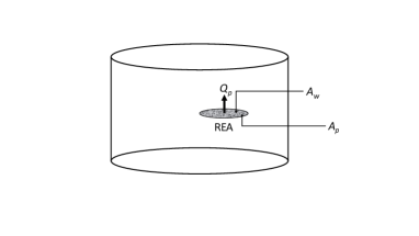
Figure 1: A Representative Elementary Area (REA) inside a porous medium plug. There is a volumetric flow rate $Q_{p}$ passing though the REA which has a transverse pore area $A_{p}$, of which an area $A_{w}$ is covered by the wetting fluid.

II.2 Some definitions

The REA has an area $A$. Part of this area is covered by the matrix material, whereas another part is covered by the pores. This latter area, $A_{p}$, we will refer to as the transverse pore area. The porosity of the REA is then given by

$$\phi=\frac{A_{p}}{A}\;.$$ (1)

There is a volumetric flow rate through the REA shown in Figure 1, $Q_{p}$. The seepage velocity of the fluids passing through the REA is then

$$v_{p}=\frac{Q_{p}}{A_{p}}\;.$$ (2)

The flow consists of a mixture of two incompressible fluids, one being more wetting with respect to the matrix than the other one. We will refer to this fluid as the “wetting fluid.” The less wetting fluid, we will refer to as the “non-wetting fluid.” Each of them is associated with a volumetric flow rate, $Q_{w}$ and $Q_{n}$, and we have

$$Q_{p}=Q_{w}+Q_{n}\;.$$ (3)

The transverse pore area of the REA may also be divide into an area associated with the wetting fluid, $A_{w}$ and an area associated with the non-wetting fluid, $A_{n}$, so that

$$A_{p}=A_{w}+A_{n}\;.$$ (4)

We may define a seepage velocity for each of the two fluids,

$$v_{w} = \frac{Q_{w}}{A_{w}}\;,$$ (5)

$$v_{n} = \frac{Q_{n}}{A_{n}}\;.$$ (6)

We define the saturations of the two fluids passing through the REA as

$$S_{w} = \frac{A_{w}}{A_{p}}\;,$$ (7)

$$S_{n} = \frac{A_{n}}{A_{p}}\;.$$ (8)

We may now combine these equations (2) —(8) to expressing the average seepage velocity as

$$v_{p}=S_{w}v_{w}+S_{n}v_{n}\;.$$ (9)

We note that could have made these definitions based on the density of the two fluids, $\rho_{w}$ and $\rho_{n}$ rather than volumes.

The porosity $\phi$, saturations $S_{w}$ and $S_{n}$, and the seepage velocities $v_{p}$, $v_{w}$ and $v_{n}$ are variables that may be associated with the chosen point surrounded by the REA. Since there for every point in the porous medium one may associate an REA, these variables, which do not depend on the size or shape of the REA, may be seen as continuous fields.

The variables we have defined should be well-defined. This is only possible if they are not fluctuating too strongly. Flooding processes typically generate fractal structures ffh22 . There are, however, length scales associated with the mechanisms controlling these structures mmhft21 , and beyond the largest of these length scales, they cease to be fractal. The same is true for steady-state flow which we consider here. We expect self averaging to take place beyond these length scales, i.e., the relative strength of the fluctuations shrinks with increasing size of the system. Hence, we assume the plug and the REAs to be large enough for the fluctuations not to dominate.

In the discussion that follows, we need to assign another property to the variables beyond being self averaging. We need them to be state variables. By this we mean that they depend on the flow properties there and then and not the history of the flow. Erpelding et al. esthfm13 studied this question experimentally and computationally, finding that this is indeed so.

A last aspect to be considered is that of hysteresis. There may indeed be hysteresis in the state variables. Knudsen and Hansen kh06 studied immiscible two-phase flow under steady-state conditions using a dynamic pore network model. They found that there are two transitions between two-phase flow and single-phase flow when the wetting saturation is the control parameter. The transition between only the non-wetting fluid moving at low saturation to both fluids moving at higher saturation does not show any hysteresis with respect to which way one passes through the transition. On the other hand, the transition between only the wetting fluid moving at high saturation and both fluids moving at lower saturation does show a strong hysteresis, see Figure 2 in Knudsen and Hansen kh06 . This hysteresis is probably caused by this transition being equivalent to a first order or a spinodal phase transition. It is well known that such transitions in ordinary equilibrium thermodynamics lead to hysteretic behavior in the state variables. Hysteretic behavior signals that there are regions of parameter space where the macroscopic state variables are multi-valued. Hence, the underlying microscopic physics has more than one locally stable mode.

II.3 Relations between the seepage velocities

Hansen et al. hsbkgv18 made the weak assumption that the volumetric flow rate through the REA is a homogeneous function of order one. That is, if we scale $A\to\lambda A$ where $\lambda$ is a scale factor, the volumetric flow rate would scale in the same way, i.e.,

$$Q_{p}(\lambda A_{w},\lambda A_{n})=\lambda Q_{p}(A_{w},A_{n})\;.$$ (10)

We have here assumed that $A_{w}$ and $A_{n}$ are independent variables. This means that that we may change the area $A$ of the REA by changing $A_{w}$, while keeping $A_{n}$ fixed or changing $A_{n}$ while keeping $A_{w}$ fixed. This makes $A$ and $A_{p}$ defined in equation (4) dependent variables. We refer to Hansen et al. hsbkgv18 for details around this.

By taking the derivative of equation (10) with respect to $\lambda$ and then setting $\lambda=1$, we find

$$Q_{p}(A_{w},A_{n})=\left(\frac{\partial Q_{p}}{\partial A_{w}}\right)_{A_{n}}A_{w}+\left(\frac{\partial Q_{p}}{\partial A_{n}}\right)_{A_{w}}A_{n}\;.$$ (11)

See Section 7.2 in Hansen et al. hsbkgv18 for a step-by-step demonstration of how these derivatives are done for a capillary fiber bundle model.

By invoking equations (2), (7) and (8), we find

$$v_{p} = \frac{Q_{p}}{A_{P}}=S_{w}\left(\frac{\partial Q_{p}}{\partial A_{w}}\right)_{A_{n}}+S_{n}\left(\frac{\partial Q_{p}}{\partial A_{n}}\right)_{A_{w}}$$ (12)

$$= S_{w}\hat{v}_{w}+S_{n}\hat{v}_{n}\;,$$

where we have defined

$$\hat{v}_{w}=\left(\frac{\partial Q_{p}}{\partial A_{w}}\right)_{A_{n}}\;,$$ (13)

$$\hat{v}_{n}=\left(\frac{\partial Q_{p}}{\partial A_{n}}\right)_{A_{w}}\;.$$ (14)

We will refer to $\hat{v}_{w}$ and $\hat{v}_{n}$ as the thermodynamic velocities.

Let us now switch to treating $S_{w}$ and $A_{p}$ as the independent variables. Simple manipulations give

$$\left(\frac{\partial}{\partial A_{w}}\right)_{A_{n}} = \left(\frac{\partial}{\partial A_{p}}\right)_{S_{w}}+\frac{S_{n}}{A_{p}}\ \left(\frac{\partial}{\partial S_{w}}\right)_{A_{p}}\;,$$ (15)

$$\left(\frac{\partial}{\partial A_{n}}\right)_{A_{w}} = \left(\frac{\partial}{\partial A_{p}}\right)_{S_{w}}-\frac{S_{w}}{A_{p}}\ \left(\frac{\partial}{\partial S_{w}}\right)_{A_{p}}\;.$$ (16)

Combining these two expressions with the definitions of the thermodynamic velocities (13) and (14) gives

$$\hat{v}_{w}=v_{p}+S_{n}\frac{dv_{p}}{dS_{w}}\;,$$ (17)

$$\hat{v}_{n}=v_{p}-S_{w}\frac{dv_{p}}{dS_{w}}\;,$$ (18)

where we note that $S_{n}$, ${\hat{v}}_{w}$, ${\hat{v}}_{n}$ and $v_{p}$ are all function of $S_{w}$ and not of $A_{p}$.

We combine equations (9) and (12),

$$v_{p}=S_{w}v_{w}+S_{n}v_{n}=S_{w}\hat{v}_{w}+S_{n}\hat{v}_{n}\;.$$ (19)

This does not imply that $v_{w}=\hat{v}_{w}$ and $\hat{v}_{n}=v_{n}$. Rather, the most general relation between them is

$$\hat{v}_{w}=v_{w}+v_{m}S_{n}\;,$$ (20)

$$\hat{v}_{n}=v_{n}-v_{m}S_{w}\;,$$ (21)

where $v_{m}$ is the co-moving velocity hsbkgv18 ; rsh20 ; rpsh22 .

Combining these two expressions with equations (17) and (18) expresses the physical seepage velocities $v_{w}$ and $v_{n}$ in terms of the average seepage velocity $v_{p}$ and the co-moving velocity $v_{m}$,

$$v_{w}=v_{p}+S_{n}\left(\frac{dv_{p}}{dS_{w}}-v_{m}\right)\;,$$ (22)

$$v_{n}=v_{p}-S_{w}\left(\frac{dv_{p}}{dS_{w}}-v_{m}\right)\;.$$ (23)

We may invert equations (22) and (23), finding

$$v_{p}=S_{w}v_{w}+S_{n}v_{n}\;,$$ (24)

$$v_{m}=S_{w}\frac{dv_{w}}{dS_{w}}+S_{n}\frac{dv_{n}}{dS_{w}}\;.$$ (25)

These four equations, (22) to (25), constitute a two-way mapping $(v_{p},v_{m})\rightleftarrows(v_{w},v_{n})$. This means that having constitutive equations for $v_{p}$ and $v_{m}$, makes it possible to derive constitutive equations for $v_{w}$ and $v_{n}$. In other theories, such as relative permeability theory, only the mapping $(v_{w},v_{n})\to v_{p}$ is given, making it impossible to start from a constitutive equation for $v_{p}$.

How to measure these variables from experimental data, see Roy et al. rpsh22 , who studied the co-moving velocity in detail using relative permeability data from the literature and from analyzing data obtained using a dynamic pore network model. They found that the co-moving velocity takes the very simple form

$$v_{m}=A+B\frac{dv_{p}}{dS_{w}}\;,$$ (26)

where $A$ and $B$ are coefficients dependent on the capillary number. It is still an open question as to why it has this simple form. We will in the following be able to give a partial answer.

With these equations, the assumption that the two fluids are incompressible and constitutive equations for $v_{p}$ and $v_{m}$, we have a closed set of equations describing the flow.

III Statistical Mechanics

III.1 Fluid configurations in a plug

We show in Figure 1 the porous plug that we discussed in Section II.1. We will center our discussion on this plug in the following.

We assume that there is a volumetric flow rate ${\cal Q}_{p}$ passing through the plug under steady-state conditions. This volumetric flow rate may be split into a wetting and a non-wetting volumetric flow rate, ${\cal Q}_{w}$ and ${\cal Q}_{n}$ so that ${\cal Q}_{p}={\cal Q}_{w}+{\cal Q}_{n}$. We use script characters to distinguish the flow through the entire plug from the flow through an REA. We show in Figure 2 three planes orthogonal to the symmetry axis of the plug, i.e., orthogonal to the average flow direction. We introduce a coordinate $z$ along the symmetry axis of the plug measuring the distance from the plug’s lower boundary to any given plane. As the sides of the plug are sealed, we have that ${\cal Q}_{p}$ is the same through the three orthogonal planes — or any other such orthogonal plane. The volumetric flow rate ${\cal Q}_{p}$ is a conserved quantity as we move along the $z$ axis. On the other hand, the volumetric flow rates of each of the two fluids, ${\cal Q}_{w}$ and ${\cal Q}_{n}$ are not conserved. Only their averages over several orthogonal planes will remain constant. One may imagine the fluids being layered in the flow direction to realize this. We also note that the transverse pore area $A_{p}$ will fluctuate from plane to plane due to fluctuations in the local porosity. The transverse area associated with the wetting fluid, $A_{w}$, will also fluctuate for two reasons: $A_{p}$ fluctuates, but more importantly because the fluid clusters fluctuate.

We pick one of the planes, assuming it is at $z_{0}$. We assume $z_{0}$ is large enough so that there are no end effects in the plane from the inlet at $z=0$. One may at each point in the plane at $z_{0}$ assign a marker for whether the point is 1. in the solid matrix, 2. in the wetting fluid or 3. in the non-wetting fluid (thus ignoring the finite thickness of the interfaces and contact lines). We also assign a velocity vector to the point, which is zero if the point is in the solid matrix. This information collected for all points in the plane at $z_{0}$ at time $t$, we will refer to as the fluid configuration ${\cal X}={\cal X}(z_{0},t)$ in this plane.

We now imagine a stack of planes. We assume the neighboring planes are a distance $dz>0$ apart.

In order to determine the flow configurations in each plane in the stack, it is not enough to know it at entry plane of the stack, $z=z_{0}$. The reason for this is that we do not know the cluster structure inside the stack. However, the configurations in each plane are still measurable.

If we move through the plug along the $z$-axis where $z_{0}\leq z\leq z_{1}$, and the plug is long enough, we will explore the space of possible configurations $\cal X$. We may do this at a fixed time $t$ (hence moving infinitely fast) or at a finite speed along the $z$-axis so that time is running. We will in both cases explore the space of possible configurations. If we choose a given plane and then average over the configurations that pass it, we will not be averaging over the matrix structure, which will be fixed in the plane. However, if we imagine an ensemble of plugs each being a realization of the same statistical pore structure, we will eventually see all configurations $\cal X$ also in this case.

This leads us directly to defining a configurational probability density ${\tilde{p}}({\cal X})$. We have also in the process sketched out an ergodicity assumption: the probability distribution for configurations in a given plane measured over an ensemble of plugs is the same as measuring it along different planes in a given plug.

Time seems to have fallen out of the description. Time keeps track of the motion of each Lagrangian fluid element as we illustrate in Figure 2. This is more information than we need. All we need is to know the fluid configurations in the planes. For this purpose, the $z$-axis acts as an effective time axis. Hence, the reference to an equivalent to the ergodic hypothesis which normally is a statement about time averaging vs. ensemble averaging.

Since we cannot reconstruct the configurations inside the stack given a knowledge of the configuration at the entry plane at $z_{0}$, one may be inclined to reject the idea to interpret the $z$-axis as an effective time direction. We point out that the same type of problem is encountered in relativistic mechanics of charged particles in strong fields where the position vs. time world lines of the particles are not single-valued functions of time f48 ; hr81 . This means that it is not possible to reconstruct the later motion of such particles from knowing their configuration at a given time.

Statistical mechanics constitutes a calculational formalism based on the knowledge of the probability distribution for configurations. The Jaynes maximum entropy principle provides a recipe for determining the configurational probability density j57 . Central to this principle is the definition of a function that quantitatively measures what we do not know about our system. This function is the Shannon entropy s48 . We construct it for the present system as

$$\Sigma_{plane}=-\int d{\cal X}{\tilde{p}}({\cal X})\ln{\tilde{p}}({\cal X})\;,$$ (27)

where the integral is over all hydrodynamically possible fluid configurations in the plane we focus on. The task is to calculate this entropy and from it determine $\tilde{p}({\cal X})$.

We will refer to the entropy defined in equation (27) as the cluster entropy. We have chosen the name as it reflects the cluster structure that the fluids are making. We emphasize that the cluster entropy is not the thermodynamic entropy defined in other work such as kbhhg19 ; kbhhg19b ; bk22 . Whereas there is production of thermodynamic entropy in the plug as we are dealing with a driven system, there is no production of cluster entropy as we are dealing with steady-state flow.

The fluid states ${\cal X}$ are not discrete. Rather, they form a continuum. Hence, we use an integral in equation (27). There are mathematical problems related to defining the measure $d{\cal X}$ is this integral. However, these difficulties we presume are of the same type encountered in ordinary statistical mechanics. We will not delve into these problems here, but rather just note their existence and that they have been solved in ordinary statistical mechanics.

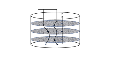
Figure 2: We show three planes orthogonal to the symmetry axis of the porous plug from Figure 1 at different $z$ coordinates. We also show the trajectories of two Lagrangian fluid elements. They started simultaneously at time $t=0$ at the plug inlet. At time $t$ they are at the indicated positions.

III.2 REA fluid configurations

We have in Section II.1 defined the REA. As for the entire plug, we may define a configuration $X$ for the REA as a hydrodynamically possible configuration within the area $A$. The configuration in the plane where the REA sits is ${\cal X}$. Hence, $X$ is a subset of $\cal X$. We also define the fluid configuration in the rest of the plane that is not part of the REA, $X_{r}$. We will refer to this part of the plane as the “reservoir.” Hence, we have that

$${\cal X}=X\cup X_{r}\;.$$ (28)

A central question is now, how independent are the configurations $X$ and $X_{r}$? If they are independent, we may focus entirely on the REA configurations $X$ as we may write the configurational probability for the entire plane as

$$\tilde{p}({\cal X})=p(X)p_{r}(X_{r})\;,$$ (29)

where $p(X)$ is the configurational probability for the REA and $p_{r}(X_{r})$ is the configurational probability for the reservoir.

Fyhn et al. fsh22 have recently studied the validity of equation (29) in a two-dimensional dynamic pore network model. By changing the size of the two-dimensional plug, while keeping the size of the REA fixed, they checked whether the statistical distributions of $Q_{p}$ and $A_{w}$ were dependent on the size of the plug. Only a very weak dependency was found which decrease with size. It is therefore realistic to assume equation (29) to be valid for large enough plugs and REAs.

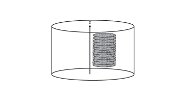
Figure 3: Averaging over a stack of REAs in the flow ($z$) direction. This ensures that the averaging is also over fluctuations in the pore structure.

We proposed in Section III.1 to view the average flow direction through the plug, the $z$-axis as a playing the role of a time axis. Averaging over time thus corresponds to averaging over a stack of REAs as shown in Figure 3. When we in the next section refer to averaging, it is averaging over this stack we mean.

We may treat the interactions between the REA and the reservoir in different ways. We may remove the REA stack from the plug and treat it as a closed-off system. This amounts to treating the REA as a plug on its own. We may leave it in the original plug, allowing it to freely interact with the reservoir. We may allow the stack to interact fully with the reservoir, but in such a way that the amount of wetting fluid is kept constant. It is not possible to implement such constraints experimentally nor computationally, but theoretically it is. The same goes for the transverse pore area: we may keep it constant theoretically, but not experimentally or computationally. Nevertheless, we will see examples of such ensembles in the following, as they correspond to different control parameters.

III.3 Jaynes maximum entropy approach

Following the Jaynes recipe, we need to maximize the cluster entropy in the REA, which is

$$\Sigma=-\int dXp(X)\ln p(X)\;,$$ (30)

under the constraints of what we know about the system. The probability density $p(X)$ is defined in equation (29).

There are three variables that we measure, the volumetric flow rate through the REA, $Q_{p}$ and the transverse pore area covered by the wetting fluid, $A_{w}$ and the transverse pore area $A_{p}$. All three of them are averages over fluctuating quantities when performed as shown in Figure 3, i.e., we average over a stack of REAs.

The average of the volumetric flow rate is

$$\int dX\ p(X)Q_{p}(X)=Q_{p}\;.$$ (31)

where the $Q_{p}(X)$ is associated with fluid configuration $X$. Likewise, the average wetting area is given by

$$\int dX\ p(X)A_{w}(X)=A_{w}\;,$$ (32)

where $A_{w}(X)$ is the wetting area associated with configuration $X$. The third variable we consider is the average transverse pore area

$$\int dX\ p(X)A_{p}(X)=A_{p}\;.$$ (33)

All three variables $Q_{p}$, $A_{w}$ and $A_{p}$ are extensive in the area of the REA, $A$. The aim now is to determine $p(X)$ based on the knowledge of these variable averages.

Following Jaynes, we use the Lagrangian multiplier technique. We start by constructing the Lagrangian which we then will maximize,

$${\cal L}= - \int dX\ p(X)\ln p(X)$$

$$- \Lambda\left(1-\int dX\ p(X)\right)$$

$$+ \lambda_{Q}\left(Q_{p}-\int dX\ p(X)Q_{p}(X)\right)$$

$$+ \lambda_{w}\left(A_{w}-\int dX\ p(X)A_{w}(X)\right)$$

$$+ \lambda_{A}\left(A_{p}-\int dX\ p(X)A_{p}(X)\right)\;,$$

with the aim to determine $p(X)$.

We assume that the three Lagrange multipliers $\lambda_{Q}$, $\lambda_{w}$ and $\lambda_{A}$ are intensive in the area of the REA, $A$. The Lagrange multiplier $\Lambda$, on the other hand, is extensive in the area $A$. It follows that the cluster entropy $\Sigma$ is extensive in $A$.

Necessary conditions for maximizing the Lagrangian (III.3) are

$$\frac{\partial{\cal L}}{\partial p(X)} = 0\;,$$ (35)

$$\frac{\partial{\cal L}}{\partial\Lambda} = 0\;,$$ (36)

$$\frac{\partial{\cal L}}{\partial\lambda_{Q}} = 0\;,$$ (37)

$$\frac{\partial{\cal L}}{\partial\lambda_{w}} = 0\;,$$ (38)

$$\frac{\partial{\cal L}}{\partial\lambda_{A}} = 0\;.$$ (39)

One may ask why not additional information is included here, such as the average wetting flow rate, $Q_{w}$? The answer to this lies in the Euler theory hsbkgv18 : there are three independent variables in the problem for which we may fix their averages. We choose here $Q_{p}$, $A_{w}$ and $A_{p}$. Other averages will then follow from the formalism we are about to develop.

Equation (35) gives

$$p(X)=e^{1-\Lambda}\ e^{-\lambda_{Q}Q_{p}(X)-\lambda_{w}A_{w}(X)-\lambda_{A}A_{p}(X)}\;,$$ (40)

and the normalization condition, equation (36) gives

$$e^{\Lambda-1}=\int dXe^{-\lambda_{Q}Q_{p}(X)-\lambda_{w}A_{w}(X)-\lambda_{A}A_{p}(X)}=Z\;,$$ (41)

where we have defined the partition function $Z=Z(\lambda_{Q},\lambda_{w},\lambda_{A})$.

We are now in a position to calculate the cluster entropy combining equations (30) and (40),

$$\Sigma = -\int p(X)\ln p(X)$$

$$= \ln Z(\lambda_{Q},\lambda_{w},\lambda_{A})+\lambda_{Q}Q_{p}+\lambda_{w}A_{w}+\lambda_{A}A_{p}\;,$$

We note that

$$Q_{p}(\lambda_{Q},\lambda_{w},\lambda_{A})=-\left(\frac{\partial\ln Z}{\partial\lambda_{Q}}\right)_{\lambda_{w},\lambda_{A}}\;,$$ (43)

$$A_{w}(\lambda_{Q},\lambda_{w},\lambda_{A})=-\left(\frac{\partial\ln Z}{\partial\lambda_{w}}\right)_{\lambda_{Q},\lambda_{A}}\;,$$ (44)

$$A_{p}(\lambda_{Q},\lambda_{w},\lambda_{A})=-\left(\frac{\partial\ln Z}{\partial\lambda_{A}}\right)_{\lambda_{Q},\lambda_{w}}\;.$$ (45)

These three equations may be solved to give $\lambda_{Q}$, $\lambda_{w}$ and $\lambda_{A}$ as functions of the three variables we know, $Q_{p}$, $A_{w}$ and $A_{p}$. They also make equation (III.3) a triple Legendre transformation, changing the control variables $\lambda_{Q}\to Q_{p}$ and $\lambda_{w}\to A_{w}$ and $\lambda_{A}\to A_{p}$. Hence, the control variables of the flow entropy are $\Sigma=\Sigma(Q_{p},A_{w},A_{p})$:

$$\Sigma(Q_{p},A_{w},A_{p})=-\int p(X)\ln p(X)$$ (46)

$$= \ln Z(\lambda_{Q},\lambda_{w},\lambda_{A})-\lambda_{Q}\left(\frac{\partial\ln Z}{\partial\lambda_{Q}}\right)_{\lambda_{w},\lambda_{A}}$$

$$- \lambda_{W}\left(\frac{\partial\ln Z}{\partial\lambda_{w}}\right)_{\lambda_{Q},\lambda_{A}}-\lambda_{A}\left(\frac{\partial\ln Z}{\partial\lambda_{A}}\right)_{\lambda_{Q},\lambda_{w}}\;,$$

We define a new variable $Q_{G}=Q_{G}(\lambda_{Q},\lambda_{w},\lambda_{A})$ through the equation

$$Z(\lambda_{Q},\lambda_{w},\lambda_{A})=e^{-\lambda_{Q}Q_{G}(\lambda_{Q},\lambda_{w},\lambda_{A})}\;.$$ (47)

It plays the role corresponding to that of a free energy in ordinary thermodynamics.

Our next step is to invert equation (III.3) so that $Q_{p}$ becomes a function of $\Sigma$ rather the other way round. That is, we transform $\Sigma(Q_{p},A_{w},A_{p})$ to $Q_{p}(\Sigma,A_{w},A_{p})$. Hence, we may write equation (III.3) or (46) as

$$Q_{G}(\lambda_{Q},\lambda_{w},\lambda_{A}) = Q_{p}(\Sigma,A_{w},A_{p})-\Sigma\frac{1}{\lambda_{Q}}$$ (48)

$$+ A_{w}\frac{\lambda_{w}}{\lambda_{Q}}+A_{p}\frac{\lambda_{A}}{\lambda_{Q}}\;,$$

where we have also used equation (47).

We see that

$$\left(\frac{\partial Q_{p}(\Sigma,A_{w},A_{p})}{\partial\Sigma}\right)_{A_{w},A_{p}}=\frac{1}{\lambda_{Q}}\;.$$ (49)

Hence, we note that the following equation, which forms part of the right hand side of equation (48), constitutes a Legendre transformation,

$$Q_{F}\left(\lambda_{Q},A_{w},A_{p}\right)=Q_{p}(\Sigma,A_{w},A_{p})-\Sigma\ \frac{1}{\lambda_{Q}}$$

$$= Q_{p}(\Sigma,A_{w},A_{p})-\Sigma\ \left(\frac{\partial Q_{p}(\Sigma,A_{w},A_{p})}{\partial\Sigma}\right)_{A_{w},A_{p}}\;.$$

Here $Q_{F}$ corresponds to another free energy in ordinary thermodynamics.

We rewrite equation (48) as

$$Q_{G}(\lambda_{Q},\lambda_{w},\lambda_{A}) - A_{p}\frac{\lambda_{A}}{\lambda_{Q}}$$

$$= Q_{F}\left(\lambda_{Q},A_{w},A_{P}\right)+A_{w}\frac{\lambda_{w}}{\lambda_{Q}}\;.$$

The left hand side of this equation constitutes a Legendre transform,

$$Q_{M}\left(\lambda_{Q},\lambda_{w},A_{p}\right)=Q_{G}(\lambda_{Q},\lambda_{w},\lambda_{A})-\frac{A_{p}}{\lambda_{Q}}\ {\lambda_{A}}\;,$$ (52)

as we have

$$\left(\frac{\partial Q_{G}(\lambda_{Q},\lambda_{w},\lambda_{A})}{\partial\left(\frac{\lambda_{A}}{\lambda_{Q}}\right)}\right)_{\lambda_{Q},\lambda_{w}}=A_{p}\;.$$ (53)

Hence, we have now transformed equation (48) to

$$Q_{M}\left(\lambda_{Q},\lambda_{w},A_{p}\right)=Q_{F}\left(\lambda_{Q},A_{w},A_{p}\right)+A_{w}\frac{\lambda_{w}}{\lambda_{Q}}\;.$$ (54)

III.4 Agiture, flow derivative and flow pressure

Let us now define three new intensive variables built from the Lagrange multipliers $\lambda_{Q}$, $\lambda_{w}$ and $\lambda_{A}$,

$$\theta = +\frac{1}{\lambda_{Q}}\;,$$ (55)

$$\pi = -\frac{\lambda_{A}}{\lambda_{Q}}\;,$$ (56)

$$\mu = -\frac{\lambda_{w}}{\lambda_{Q}}\;.$$ (57)

The first one, $\theta$, by its resemblance to temperature in ordinary statistical mechanics, we will name the agiture. The unit of the agiture is the same as volumetric flow rate. However, it is an intensive variable.

The second one, $\pi$, we will name the flow pressure. This variable is the conjugate of the flow area $A_{p}$,

$$\pi = \left(\frac{\partial Q_{F}(\theta,A_{w},A_{p})}{\partial A_{p}}\right)_{\theta,A_{w}}$$ (58)

$$= \left(\frac{\partial Q_{p}(\Sigma,A_{w},A_{p})}{\partial A_{p}}\right)_{\Sigma,A_{w}}\;.$$

The unit of $\pi$ is inverse velocity. Referring to equation (1), we see that $A_{p}$ is a measure of the porosity $\phi$ and $\pi$ is therefore a velocity variable conjugate to the porosity.

The third variable, equation (57) we name the flow derivative. We will explain the name in the next section. As $\pi$, its unit is that of a velocity. It is the conjugate of the transversal wetting fluid area $A_{w}$,

$$\mu = \left(\frac{\partial Q_{F}(\theta,A_{w},A_{p})}{\partial A_{w}}\right)_{\theta,A_{p}}$$ (59)

$$= \left(\frac{\partial Q_{p}(\Sigma,A_{w},A_{p})}{\partial A_{w}}\right)_{\Sigma,A_{p}}\;.$$

playing a role similar to a chemical potential in ordinary statistical mechanics. Through equation (7), we see that the flow derivative is the conjugate of the wetting saturation $S_{w}$.

III.5 Connection with Euler homogeneity approach

We need to define one more variable,

$$Q_{N}(\Sigma,\mu,A_{p})=Q_{M}\left(\theta,\mu,A_{p}\right)-\Sigma(\theta,\mu,A_{p})\theta\;,$$ (60)

where

$$\Sigma(\theta,\mu,A_{p})=\left(\frac{\partial Q_{M}(\theta,\mu,A_{p})}{\partial\theta}\right)_{\mu,A_{p}}\;.$$ (61)

Combining this definition with equations (III.3) and (54) gives

$$Q_{N}\left(\Sigma,\mu,A_{p}\right)=Q_{p}\left(\Sigma,A_{w},A_{p}\right)-A_{w}\mu\;.$$ (62)

We use the fact that both $Q_{N}(\Sigma,\mu,A_{p})$ and $Q_{p}(\Sigma,A_{w},A_{p})$ are homogeneous functions of order one in the extensive variables $\Sigma$, $A_{w}$ and $A_{p}$,

$$Q_{N}\left(\lambda\Sigma,\mu,\lambda A_{p}\right) = \lambda Q_{N}\left(\Sigma,\mu,A_{p}\right)\;,$$ (63)

$$Q_{p}\left(\lambda\Sigma,\lambda A_{w},\lambda A_{p}\right) = \lambda Q_{p}\left(\Sigma,A_{w},A_{p}\right)\;.$$ (64)

We now set $\lambda=1/A_{p}$ and combine these two expressions with equation (62), finding

$$A_{p}Q_{N}\left(\sigma,\mu,1\right)=A_{p}Q_{p}\left(\sigma,S_{w},1\right)-A_{w}\mu\;,$$ (65)

where we also have used equation (7) and we have defined the cluster entropy density

$$\sigma=\frac{\Sigma}{A_{p}}\;.$$ (66)

We now divide equation (65) by $A_{p}$, noting that

$$Q_{N}\left(\sigma,\mu,1\right) = v_{N}(\sigma,\mu)\;,$$ (67)

$$Q_{p}(\sigma,S_{w},1) = v_{p}(\sigma,S_{w})\;,$$ (68)

i.e., $v_{N}$ and $v_{p}$ are velocities. We recognize $v_{p}=Q_{p}/A_{p}$ from equation (2) as the average seepage velocity of the two fluids. Equation (65) then takes on the form

$$v_{N}(\sigma,\mu)=v_{p}(\sigma,S_{w})-S_{w}\mu\;.$$ (69)

Let us now go back to equation (59) and use scaling relation (64) to find

$$\left(\frac{\partial v_{p}(\sigma,S_{w})}{\partial S_{w}}\right)_{\sigma}=\mu\;.$$ (70)

This expression is the reason why we name $\mu$ the flow derivative. We now compare these two equations (69) and (70) to equation (21), which we reproduce here:

$${\hat{v}}_{n}=v_{p}-S_{w}\left(\frac{dv_{p}}{dS_{w}}\right)\;.$$

This equation is one of the central results derived by Hansen et al. hsbkgv18 . By comparison, we identify

$$v_{N}={\hat{v}}_{n}\;,$$ (71)

where the thermodynamic velocity of the non-wetting fluid, ${\hat{v}}_{n}$, is defined in equation (14). Equation (69) may be written

$${\hat{v}}_{n}(\sigma,\mu)=v_{p}(\sigma,S_{w}(\sigma,\mu))-S_{w}(\sigma,\mu)\mu\;,$$ (72)

and we have that

$$S_{w}(\sigma,\mu)=-\left(\frac{\partial{\hat{v}}_{n}(\sigma,\mu)}{\partial\mu}\right)_{\sigma}\;.$$ (73)

These two equations are our central result. It demonstrates that the thermodynamic velocity of the non-wetting fluid is the Legendre transform of the average seepage velocity with respect to the wetting saturation and that the wetting saturation is minus the derivative of the non-wetting thermodynamic velocity with respect to the flow derivative. Equation (21) was derived based on the volumetric flow rate being a homogeneous function of the first kind in the transverse pore area. Now, we see this equation as a fundamental equation resulting from an underlying statistical mechanics, with variables $(\theta,\Sigma)$ and $(\mu,S_{w})$, and $(\pi,\phi)$ forming conjugate pairs.

III.6 Partition functions

The partition function is given by

$$Z(\theta,\mu,\pi)=\int\ dX\ e^{-Q_{p}(X)/\theta+\mu A_{w}(X)/\theta+\pi A_{p}(X)/\theta}\;.$$ (74)

We may split the integration over states $X$ into an integral over $A_{p}$ and then over all states $X$ that has a given $A_{p}$,

$$Z(\theta,\mu,\pi) = e^{-Q_{G}(\theta,\mu,\pi)/\theta}$$ (75)

$$= \int_{0}^{A}\ dA_{p}e^{\pi A_{p}/\theta}\ Z(\theta,\mu,A_{p})\;,$$

where we have defined

$$Z(\theta,\mu,A_{p})$$

$$= \int\ dX\ \delta(A_{p}(X)-A_{p})\ e^{-Q_{p}(X)/\theta+\mu A_{w}(X)/\theta}$$

$$= \frac{1}{A}\int\ dX\ \delta(\phi(X)-\phi)\ e^{-Q_{p}(X)/\theta+\mu A_{w}(X)/\theta}\;,$$

and where $\delta(\cdots)$ is the Dirac delta-function. We have used that $A\phi=A_{p}$, see equation (1). We have that

$$Z(\theta,\mu,A_{p})=\frac{1}{A}\ e^{-Q_{M}(\theta,\mu,A_{p})/\theta}\;,$$ (77)

where $Q_{M}(\theta,\mu,A_{p})$ is defined in equation (62).

We may now write partition function $Z(\theta,\mu,A_{p})$ in equation (III.6) as

$$Z(\theta,\mu,A_{p})=\int_{0}^{A_{p}}\ dA_{w}\ e^{\mu A_{w}/\theta}Z(\theta,A_{w},A_{p})\;,$$ (78)

where we have defined

$$Z(\theta,A_{w},A_{p})$$

$$= \int\ dX\ \delta(A_{w}(X)-A_{w})\ \delta(A_{p}(X)-A_{p})e^{-Q_{p}(X)/\theta}\;,$$

$$= \int\ \frac{dX}{A_{p}\ A}\ \delta(S_{w}(X)-S_{w})\ \delta(\phi(X)-\phi)e^{-Q_{p}(X)/\theta}\;,$$

which we may write as

$$Z(\theta,A_{w},A_{p})=\frac{1}{A_{p}\ A}\ e^{-Q_{F}(\theta,A_{w},A_{p})/\theta}\;.$$ (80)

We may repeat this procedure one more time. We rewrite the partition function $Z(\theta,A_{w},A_{p})$, equation (III.6) as

$$Z(\theta,A_{w},A_{p})=\int_{-\infty}^{+\infty}\ dQ_{p}e^{-Q_{p}/\theta}\ Z(Q_{p},A_{w},A_{p})\;,$$ (81)

where

$$Z(Q_{p},A_{w},A_{p})=\int\ dX\$$

$$\delta(Q_{p}(X)-Q_{p})\ \delta(A_{w}(X)-A_{w})\ \delta(A_{p}(X)-A_{p})\;.$$

This microcanonical partition function (as $Q_{p}$ is the control variable) is also the (unnormalized) density of states with respect to the variables $Q_{p}$, $A_{w}$ and $A_{p}$. It demonstrates that all states $X$ with the same $Q_{p}$, $A_{w}$ and $A_{p}$ are equally probable. This brings us back to our starting point: the entropy has its maximum when all states that comply with the constraints (31), (32) and (33) are equally probable.

III.7 Co-moving velocity

The co-moving velocity, which is defined in equations (20) and (21), constitutes the bridge between the seepage velocities, equations (5) and (6), and the thermodynamics velocities, equations (13) and (14). By combining the defining equations for the co-moving velocities with the two equations ensuing from the Euler scaling assumption for the volumetric flow rate, we express the seepage velocity of the two fluid species in terms of the average seepage velocity and the co-moving velocity in equations (22) and (23).

Combining equation (23) with equation (73) based on statistical mechanics, we find a consistent structure

$$v_{n}(\sigma,\mu)=v_{p}\left(\sigma,S_{w}(\sigma,\mu)\right)-S_{w}(\sigma,\mu)\left(\mu-v_{m}(\sigma,\mu)\right)\;,\\$$ (83)

when assuming that $v_{n}=v_{n}(\sigma,\mu)$ and $v_{m}=v_{m}(\sigma,\mu)$. Thus, we have expressed the physical seepage velocity for the non-wetting fluid within the pseudo-thermodynamic formalism we are developing. The corresponding physical seepage velocity for the wetting fluid may then be found e.g. by using equation (9).

The phenomenological form found by Roy et al. rpsh22 , equation (26), is consistent with the assumption for $v_{m}$, as equation (26) then takes the form

$$v_{m}(\sigma,\mu)=A(\sigma)+B(\sigma)\mu\;,$$ (84)

with

$$B(\sigma)=\left(\frac{\partial v_{m}(\sigma,\mu)}{\partial\mu}\right)_{\sigma}\;.$$ (85)

We note that the dependence of $A$ and $B$ on the capillary number is consistent with the two coefficients depending on the cluster entropy density $\sigma$.

Why $v_{m}$ is linear in $\mu$ is not known.

III.8 Maxwell relations

We now see that the Euler homogeneity approach of Hansen et al. hsbkgv18 was just the tip of an iceberg. Having anchored the approach in a statistical mechanics, we now have access to a rich formalism that parallels thermodynamics.

For example, we find the equivalents of the Maxwell relations in ordinary thermodynamics. We derive just one in the following.

We have that

$$\left(\frac{\partial Q_{F}(\theta,A_{w},A_{p})}{\partial\theta}\right)_{A_{w},A_{p}}=\Sigma\;.$$ (86)

We combine this equation with equation (59), taking the cross derivatives, and finding

$$\left(\frac{\partial\Sigma}{\partial A_{w}}\right)_{\theta,A_{p}}=\left(\frac{\partial\mu}{\partial\theta}\right)_{A_{w},A_{p}}\;,$$ (87)

which may be written as

$$\left(\frac{\partial\sigma}{\partial S_{w}}\right)_{\theta}=\left(\frac{\partial\mu}{\partial\theta}\right)_{S_{w}}\;.$$ (88)

IV Fluctuations and agiture

Our starting point are equations (41) and (47), i.e.,

$$Q_{G}(\theta,\mu,\pi)=-\theta\ln[Z(\theta,\mu,\pi)]$$

$$= -\theta\ln\left[\int dXe^{-Q_{p}(X)/\theta+\mu A_{w}(X)/\theta+\pi A_{p}(X)/\theta}\right]\;.$$

This immediately gives

$$\left(\frac{\partial Q_{G}(\theta,\mu,\pi)}{\partial\mu}\right)_{\theta,\pi}$$ (90)

$$= \frac{1}{Z}\int dXA_{w}(X)e^{-Q_{p}(X)/\theta+\mu A_{w}(X)/\theta+\pi A_{p}(X)/\theta}$$

$$= A_{w}\;.$$

Taking the derivative a second time with respect to $\mu$ gives

$$- \theta\left(\frac{\partial^{2}Q_{G}(\theta,\mu,\pi)}{\partial\mu^{2}}\right)_{\theta,\pi}$$ (91)

$$= \frac{1}{Z}\int dXA_{w}^{2}(X)e^{-Q_{p}(X)/\theta+\mu A_{w}(X)/\theta+\pi A_{p}(X)/\theta}$$

$$- \left[\frac{1}{Z}\int dXA_{w}(X)e^{-Q_{p}(X)/\theta+\mu A_{w}(X)/\theta+\pi A_{p}(X)/\theta}\right]^{2}$$

$$= \langle A_{w}^{2}\rangle-A_{w}^{2}=\Delta A_{w}^{2}\;,$$

where we have defined the fluctuations $\Delta A_{w}^{2}$. We now combine equations (1) and (7) to find

$$A_{w}=A\ \frac{A_{p}}{A}\ \frac{A_{w}}{A_{p}}=A\phi S_{w}\;.$$ (92)

This allows us to transform equation (91) into

$$\Delta(\phi S_{w})^{2}=\frac{\theta}{A}\left(\frac{\partial(\phi S_{w})}{\partial\mu}\right)_{\theta,\pi}\;.$$ (93)

We see that the agiture $\theta$ seems proportional to the fluctuations $\Delta(\phi S_{w})^{2}$. However, due to the term $(\partial\phi S_{w}/\partial\mu)_{\theta,\pi}$, the relation between them is complex. We may calculate the porosity fluctuations by taking the partition function $Z(\theta,\mu,\pi)$, equation (74), as starting point. We find

$$\Delta\phi^{2}=\frac{\theta}{A}\ \left(\frac{\partial\phi}{\partial\pi}\right)_{\theta,\mu}\;,$$ (94)

where

$$\Delta\phi^{2}=\frac{1}{A^{2}}\left[\langle A_{p}(X)^{2}\rangle-A_{p}^{2}\right]\;.$$ (95)

We note that the porosity field $\phi$ is a property of the matrix and not the flow. Hence, equation (94) gives a direct link between the agiture $\theta$ and the flow pressure $\pi$,

$$\theta=A\Delta\phi^{2}\ \left(\frac{\partial\pi}{\partial\phi}\right)_{\theta,\mu}\;.$$ (96)

V Conditions for steady state in a heterogeneous plug

We consider in the following the conditions for steady state in a heterogeneous plug.

We show in Figure 4 a plug that is divided into a region A and a region B, which have different matrix properties. The difference may for example be that the wetting properties of the matrix in region A differ from those of region B. The full system, which consists of both regions A and B, is a closed system.

We will in the following focus on the four quantities $Q_{p}$, $A_{w}$, $A_{p}$ and $\Sigma$ that describe the flow in the plug. Strictly speaking, we should change our notation, e.g., $Q_{p}\to{\cal Q}_{p}$, since we are considering the entire plug. However, in order to avoid complicating the notation and therefore making the material less accessible, we refrain from making the change.

These four quantities are extensive, i.e., additive. This means that we may express them in terms of the two regions A and B. We have

$$Q_{p}=Q_{p}^{A}+Q_{p}^{B}\;,$$ (97)

$$\Sigma=\Sigma^{A}+\Sigma^{B}\;,$$ (98)

$$A_{w}=A_{w}^{A}+A_{w}^{B}\;,$$ (99)

$$A_{p}=A_{p}^{A}+A_{p}^{B}\;.$$ (100)

We write $Q_{p}$ in terms of the control variables $\Sigma$, $A_{w}$ and $A_{p}$,

$$Q_{p}(\Sigma,A_{w},A_{p})=Q_{p}^{A}(\Sigma^{A},A_{w}^{A},A_{p}^{A})+Q_{p}^{B}(\Sigma^{B},A_{w}^{B},A_{p}^{B})\;.$$ (101)

Since the total volumetric flow rate is conserved in the plug, we must have that fluctuations in it must be zero, i.e,

$$\delta Q_{p}=\delta Q_{p}^{A}+\delta Q_{p}^{B}=0\;.$$ (102)

The fluctuations in $Q_{p}^{A}$ and $Q_{p}^{B}$ come from fluctuations in $\Sigma^{A}$ and $\Sigma^{B}$, $A_{w}^{A}$ and $A_{w}^{B}$, and $A_{p}^{A}$ and $A_{p}^{B}$. We express $\delta Q_{p}^{A}$ and $\delta Q_{p}^{B}$ in terms of the fluctuations of these variables,

$$\delta Q_{p}^{A}(\Sigma^{A},A_{w}^{A},A_{p}^{A})$$

$$= \left(\frac{\partial Q_{p}^{A}(\Sigma^{A},A_{w}^{A},A_{p}^{A})}{\partial\Sigma^{A}}\right)_{A_{w}^{A},A_{p}^{A}}\ \delta\Sigma^{A}$$

$$+ \left(\frac{\partial Q_{p}^{A}(\Sigma^{A},A_{w}^{A},A_{p}^{A})}{\partial A_{w}^{A}}\right)_{\Sigma^{A},A_{p}^{A}}\ \delta A_{w}^{A}$$

$$+ \left(\frac{\partial Q_{p}^{A}(\Sigma^{A},A_{w}^{A},A_{p}^{A})}{\partial A_{p}^{A}}\right)_{\Sigma^{A},A_{w}^{A}}\ \delta A_{p}^{A}\;.$$

Likewise, we have

$$\delta Q_{p}^{B}(\Sigma^{B},A_{w}^{B},A_{p}^{B})$$

$$= \left(\frac{\partial Q_{p}^{B}(\Sigma^{B},A_{w}^{B},A_{p}^{B})}{\partial\Sigma^{B}}\right)_{A_{w}^{B},A_{p}^{B}}\ \delta\Sigma^{B}$$

$$+ \left(\frac{\partial Q_{p}^{B}(\Sigma^{B},A_{w}^{B},A_{p}^{B})}{\partial A_{w}^{B}}\right)_{\Sigma^{B},A_{p}^{B}}\ \delta A_{w}^{B}$$

$$+ \left(\frac{\partial Q_{p}^{B}(\Sigma^{B},A_{w}^{B},A_{p}^{B})}{\partial A_{p}^{B}}\right)_{\Sigma^{B},A_{w}^{B}}\ \delta A_{p}^{B}\;.$$

There is no production of cluster entropy as this entropy is at a maximum. However, cluster entropy may move between regions A and B. Hence, we have

$$\delta\Sigma=\delta\Sigma^{A}+\delta\Sigma^{B}=0\;.$$ (105)

Furthermore, we keep the control variables $A_{w}$ and $A_{p}$ fixed. This is of course not possible experimentally. However, as a theoretical concept, it is permissible. Hence, we have that

$$\delta A_{w}=\delta A_{w}^{A}+\delta A_{w}^{B}=0\;,$$ (106)

$$\delta A_{p}=\delta A_{p}^{A}+\delta A_{p}^{B}=0\;.$$ (107)

We now combine equations (102) — (107) to find

$$\delta Q_{p}(\Sigma,A_{w},A_{p})$$

$$= \left[\left(\frac{\partial Q_{p}^{A}}{\partial\Sigma^{A}}\right)_{A_{w}^{A},A_{p}^{A}}-\left(\frac{\partial Q_{p}^{B}}{\partial\Sigma^{B}}\right)_{A_{w}^{B},A_{p}^{B}}\right]\delta\Sigma^{A}$$

$$+ \left[\left(\frac{\partial Q_{p}^{A}}{\partial A_{w}^{A}}\right)_{\Sigma^{A},A_{p}^{A}}-\left(\frac{\partial Q_{p}^{B}}{\partial A_{w}^{B}}\right)_{\Sigma^{B},A_{p}^{B}}\right]\delta A_{w}^{A}$$

$$+ \left[\left(\frac{\partial Q_{p}^{A}}{\partial A_{p}^{A}}\right)_{\Sigma^{A},A_{w}^{A}}-\left(\frac{\partial Q_{p}^{B}}{\partial A_{p}^{B}}\right)_{\Sigma^{B},A_{w}^{B}}\right]\delta A_{p}^{A}=0\;.$$

We now assume that the cluster entropy fluctuations $\delta\Sigma^{A}$ are independent of the fluctuations in $\delta A_{w}^{A}$ and $\delta A_{p}^{A}$. This leads to

$$\theta^{A} = \left(\frac{\partial Q_{p}^{A}(\Sigma^{A},A_{w}^{A},A_{p}^{A})}{\partial\Sigma^{A}}\right)_{A_{w}^{A},A_{p}^{A}}$$

$$= \left(\frac{\partial Q_{p}^{B}(\Sigma^{B},A_{w}^{B},A_{p}^{B})}{\partial\Sigma^{B}}\right)_{A_{w}^{B},A_{p}^{B}}=\theta^{B}\;,$$

where we have used equations (49) and (55).

If we now furthermore assume that the fluctuations in $\delta A_{w}^{A}$ and $\delta A_{p}^{A}$ are uncorrelated, we find

$$\mu^{A} = \left(\frac{\partial Q_{p}^{A}(\Sigma^{A},A_{w}^{A},A_{p}^{A})}{\partial A_{w}^{A}}\right)_{\Sigma^{A},A_{p}^{A}}$$

$$= \left(\frac{\partial Q_{p}^{B}(\Sigma^{B},A_{w}^{B},A_{p}^{B})}{\partial A_{w}^{B}}\right)_{\Sigma^{B},A_{p}^{B}}=\mu^{B}\;,$$

and

$$\pi^{A} = \left(\frac{\partial Q_{p}^{A}(\Sigma^{A},A_{w}^{A},A_{p}^{A})}{\partial A_{p}^{A}}\right)_{\Sigma^{A},A_{w}^{A}}$$

$$= \left(\frac{\partial Q_{p}^{B}(\Sigma^{B},A_{w}^{B},A_{p}^{B})}{\partial A_{p}^{B}}\right)_{\Sigma^{B},A_{w}^{B}}=\pi^{B}\;.$$

These three criteria for steady state flow, equations (V), (V) and (V), are analogous to the criteria for two open systems in thermal contact and in equilibrium: here the temperature, pressure and the chemical potential must be the same.

It is important to point out the following. In ordinary thermodynamics, the rule is that the conjugate of a conserved quantity is constant in a heterogeneous system at equilibrium. This is e.g., the argument for the temperature being the same everywhere in the system at equilibrium as the entropy is at a maximum. This is the same argument as we have used here which leads to equation (V). However, consider two magnets with different magnetic susceptibilities in contact which is placed in a uniform magnetic field $H$. The conjugate of the magnetization $M$, which is the magnetic flux $B$, is not equal in the two magnets in contact, $B^{A}\neq B^{B}$. What goes wrong here is that it is not possible to let magnetization fluctuate between the two magnets so that its sum is constant, i.e., $\delta M^{A}=-\delta M^{B}$ while simultaneously keeping the total internal energy and the total entropy constant, i.e., $\delta U=\delta U^{A}+\delta U^{B}=0$ and $\delta S=\delta S^{A}+\delta S^{B}=0$. In our system — steady-state two-phase flow in a porous medium — the following question then becomes central: is it possible to fulfill $\delta Q_{p}=0$ and $\delta\Sigma=0$, and at the same time have $\delta A_{w}^{A}=-\delta A_{w}^{B}$ and $\delta A_{p}^{A}=-\delta A_{p}^{B}$? The answer to this question is not obvious. Only experiments or computations on models may provide an answer. If the answer is no, only equation (V) will be valid, and not equations (V) and (V).

What about the pressure gradient? We must have that

$$\nabla P^{A}=\nabla P^{B}$$ (112)

for steady-state conditions to apply. If the two pressure gradients were different, a pressure gradient orthogonal to the flow direction would develop, which would then divert the flow from the $z$ direction, breaking the assumption of steady-state flow.

Equation (112) is fulfilled if we have that

$$|\nabla P|=|\nabla P|(\theta,\mu,\pi)\;,$$ (113)

due to (V), and if (V) and (V) are valid.

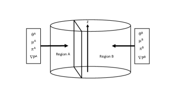
Figure 4: The plug is now divided into a region A and a region B which differ in composition. The flow in region A is characterized by the variables $\theta^{A}$, $\mu^{A}$, $\pi^{A}$ and $\nabla P^{A}$, whereas in region B we have $\theta^{B}$, $\mu^{B}$, $\pi^{B}$ and $\nabla P^{B}$. Steady state flow is attained when $\theta^{A}=\theta^{B}$ and $\mu^{A}=\mu^{B}$ and $\pi^{A}=\pi^{B}$ according to equations (V), (V) and (V). In addition we have $\nabla P^{A}=\nabla P^{B}$.

VI Discussion and Conclusion

A central problem in the physics of porous media is how to scale up knowledge of the physics at the pore level to the continuum scale, often referred to as the Darcy scale, where the pores are negligible in size. The notion of up-scaling is of course only meaningful if we know which coarse-scale physics we are up-scaling to, and the traditional relative permeability theory has well known weak points. The theory of Hansen et al. hsbkgv18 is a radically different approach to the coarse-scale physics. This theory is formally similar to some parts of thermodynamics, but it is the flow rates, and the relations between flow rates, that are the central players. In its core the theory is based on the volumetric flow rate being an Euler homogeneous function.

In the present paper, we have developed a statistical mechanics framework for immiscible incompressible two-phase flow. In this framework, total flow rate plays the same role as energy in ordinary statistical mechanics, and local steady state flow plays the role of local thermodynamic equilibrium. We have shown that the pseudo-thermodynamics that follows from the statistical mechanics framework extends the earlier theory of Hansen et al. hsbkgv18 , rendering it a complete pseudo-thermodynamics in the spirit of Edwards and Oakeshot’s pseudo-thermodynamics for powders eo89 .

In the same way that ordinary statistical mechanics serves as a tool for calculating macro-scale properties from known molecular scale physics, the present statistical mechanics links the pore scale hydrodynamic description to a continuum scale physics, thus solving the up-scaling problem. The key link is the partition function $Z(\theta,\mu,\pi)$ defined in equation (41). The integral is over all physical fluid configurations, and he physics sits in the measure $dX$ over configurations and pore structure.

The up-scaling from the intermittent flow of fluid clusters through pore space to a description with a small number of continuum scale variables admits an immense level of ignorance. This ignorance is reflected in the pseudo-thermodynamics as the cluster entropy. We call the conjugate variable to this cluster entropy the agiture. The agiture measure the level of agitation in the flow. Typically a high agiture is associated with high flow rates, in the same way high temperature is associated with high energies in thermal systems.

We have not proposed here any technique as to how the agiture $\theta$ may be measured, or controlled, experimentally or computationally. The flow pressure $\pi$ seems also difficult to measure. Measuring the flow derivative is, on the other hand, seemingly easier to measure. In terms of the average seepage velocity and the saturation, it may be written

$$\mu=\left(\frac{\partial v_{p}(\sigma,S_{w})}{\partial S_{w}}\right)_{\sigma}\;.$$ (114)

Since we are assuming steady-state flow, the cluster entropy is at a maximum and therefore constant.

We also note that we have used five different ensembles in this work, where control parameters are respectively

$$(\theta,\mu,\pi)\;,$$

$$(\theta,\mu,A_{p})\;,$$

$$(\Sigma,\mu,A_{p})\;,$$

$$(\theta,A_{w},A_{p})\;,$$

$$(\Sigma,A_{w},A_{p})\;.$$

The first of these ensembles is easily realizable experimentally as this describes an REA communicating freely with the rest of the porous medium. The second one, with $A_{p}$ controlled, is feasible e.g. by using 3D printing techniques to construct the porous medium. The two last three ensembles must be seen as theoretical constructs. We note, however, that this is standard procedure in thermodynamics in that one always starts with the Gibbs relation, which relates variations in the internal energy to variations in the extensive variables irrespective of whether this ensemble is accessible experimentally or not.

We see that a steady-state condition in a heterogeneous porous medium such as that shown in Figure 4 is that the agiture is constant throughout the entire system, equation (V). On the other hand, the two additional equilibrium conditions, equations (V) and (V), hinge on additional assumptions that need to be verified experimentally or computationally. In light of the above discussion, verifying the validity of equation (V) is the easier one of the three equations.

The probability to find a flow configuration $p(X)$ in the REA which is the central to the theory we present here. It was emphasized at the beginning of Section III.3 that the fluid configuration $X$ refers to the configuration in the REA, not the entire plane cutting through the plug, ${\cal X}=X\cup X_{r}$. It is crucial for the theory that $p(X)$ does not depend on the properties of the entire plug. Recent numerical work by Fyhn et al. fsh22 indicates that this is indeed correct.

Given all these caveats and open question, the fact remains that the framework we have presented here, opens up for viewing immiscible two-phase flow in porous media in a different way than before. We have here divided the problem into 1. constructing a framework by which the concepts that are necessary are put in place, and 2. connecting these concepts to the underlying fluid dynamics and thermodynamics. This paper accomplishes the first goal.

References

- (1) J. Bear, Dynamics of Fluids in Porous Media (Dover, Mineola, 1988).
- (2) M. Sahimi, Flow and transport in porous media and fractured rock: from classical methods to modern approaches, (Wiley, New York, 2011); doi.org/10.1002/9783527636693.
- (3) M. J. Blunt, Multiphase flow in permeable media (Cambridge Univ. Press, Cambridge, 2017).
- (4) J. Feder, E. G. Flekkøy and A. Hansen, Physics of flow in porous media, (Cambridge Univ. Press, Cambridge, 2022); ISBN 9781108989114.
- (5) R. D. Wyckoff and H. G. Botset, The flow of gas-liquid mixtures through unconsolidated sands, Physics 7, 325 (1936); doi.org/10.1063/1.1745402.
- (6) S. M. Hassanizadeh and W. G. Gray, Mechanics and thermodynamics of multiphase flow in porous media including interphase boundaries, Adv. Water Res. 13, 169 (1990).
- (7) S. M. Hassanizadeh and W. G. Gray, Towards an improved description of the physics of two-phase flow, Adv. Water Res. 16, 53 (1993).
- (8) S. M. Hassanizadeh and W. G. Gray, Thermodynamic basis of capillary pressure in porous media, Water Resour. Res. 29, 3389 (1993).
- (9) J. Niessner, S. Berg and S. M. Hassanizadeh, Comparison of two-phase Darcy’s law with a thermodynamically consistent approach, Transp. Por. Med. 88, 133 (2011).
- (10) W. G. Gray and C. T. Miller, Introduction to the thermodynamically constrained averaging theory for porous medium systems (Springer Verlag, Berlin, 2014).
- (11) S. Whitaker, Flow in porous media II: The governing equations for immiscible, two-phase flow, Transp. Por. Med. 1, 105 (1986); doi.org/10.1007/BF00714688.
- (12) S. Kjelstrup, D. Bedeaux, A. Hansen, B. Hafskjold and O. Galteland, Non-isothermal transport of multi-phase fluids in porous media. the entropy production, Front. Phys. 6, 126 (2018); doi.org/10.3389/fphy.2018.00126.
- (13) S. Kjelstrup, D. Bedeaux, A. Hansen, B. Hafskjold and O. Galteland, Non-isothermal transport of multi-phase fluids in porous media. Constitutive equations, Front. Phys. 6, 150 (2019); doi.org/10.3389/fphy.2018.00150.
- (14) D. Bedeaux and S. Kjelstrup, Fluctuation-dissipiation theorems for multiphase flow in porous media, Entropy, 24, 46 (2022); doi.org/10.3390/e24010046.
- (15) R. Hilfer and H. Besserer, Macroscopic two-phase flow in porous media, Physica B, 279, 125 (2000); doi.org/10.1016/S0921-4526(99)00694-8.
- (16) R. Hilfer, Capillary pressure, hysteresis and residual saturation in porous media, Physica A, 359, 119 (2006); doi.org/10.1016/j.physa.2005.05.086.
- (17) R. Hilfer, Macroscopic capillarity and hysteresis for flow in porous media, Phys. Rev. E, 73, 016307 (2006); doi.org/10.1103/PhysRevE.73.016307.
- (18) R. Hilfer, Macroscopic capillarity without a constitutive capillary pressure function, Physica A, 371, 209 (2006); doi.org/10.1016/j.physa.2006.04.051.
- (19) R. Hilfer and F. Döster, Percolation as a basic concept for capillarity, Transp. Por. Med. 82, 507 (2010); doi.org/10.1007/s11242-009-9395-0.
- (20) F. Döster, O. Hönig and R. Hilfer, Horizontal flow and capillarity-driven redistribution in porous media, Phys. Rev. E, 86, 016317 (2012); doi.org/10.1103/PhysRevE.86.016317.
- (21) M. S. Valavanides, G. N. Constantinides and A. C. Payatakes, Mechanistic Model of steady-state two-phase flow in porous media based on ganglion dynamics, Transp. Por. Med. 30, 267 (1998); doi.org/10.1023/A:1006558121674.
- (22) M. S. Valavanides, Steady-state two-phase flow in porous media: review of progress in the development of the DeProF theory bridging pore- to statistical thermodynamics-scales, Oil Gas Sci. Technol. 67, 787 (2012); doi.org/10.2516/ogst/2012056.
- (23) M. S. Valavanides, Review of steady-state two-phase flow in porous media: independent variables, universal energy efficiency map, critical flow conditions, effective characterization of flow and pore network, Transp. Porous Media, 123, 45 (2018); doi.org/10.1007/s11242-018-1026-1.
- (24) A. Hansen, S. Sinha, D. Bedeaux, S. Kjelstrup, M. A. Gjennestad and M. Vassvik, Relations between seepage velocities in immiscible, incompressible two-phase flow in porous Media, Transp. Por. Med. 125, 565 (2018); doi.org/10.1007/s11242-018-1139-6.
- (25) S. Roy, S. Sinha and A. Hansen, Flow-area relations in immiscible two-phase flow in porous media, Front. Phys. 8, 4 (2020); doi.org/10.3389/fphy.2020.00004.
- (26) S. Roy, H. Pedersen, S. Sinha and A. Hansen, The Co-moving Velocity in immiscible two-phase flow in porous media, arXiv:2108.10187, to appear in Transp. Por. Med. (2022).
- (27) K. T. Tallakstad, H. A. Knudsen, T. Ramstad, G. Løvoll, K. J. Måløy, R. Toussaint and E. G. Flekkøy, Steady-state two-phase flow in porous media: statistics and transport properties, Phys. Rev. Lett. 102, 074502 (2009); doi.org/ 10.1103/PhysRevLett.102.074502.
- (28) K. T. Tallakstad, G. Løvoll, H. A. Knudsen, T. Ramstad, E. G. Flekkøy and K. J. Måløy, Steady-state simultaneous two-phase flow in porous media: an experimental study, Phys. Rev. E 80, 036308 (2009); doi.org/10.1103/PhysRevE.80.036308.
- (29) O. Aursjø, M. Erpelding, K. T. Tallakstad, E. G. Flekkøy, A. Hansen and K. J. Måløy, Film flow dominated simultaneous flow of two viscous incompressible fluids through a porous medium, Front. Phys. 2, 63 (2014); doi.org/10.3389/fphy.2014.00063.
- (30) S. Sinha, A. T. Bender, M. Danczyk, K. Keepseagle, C. A. Prather, J. M. Bray, L. W. Thrane, J. D. Seymour, S. L. Codd and A. Hansen, Effective rheology of two-phase flow in three-dimensional porous media: experiment and simulation, Transp. Por. Med. 119, 77-94 (2017); doi.org/10.1007/s11242-017-0874-4.
- (31) Y. Gao, Q. Lin, B. Bijeljic and M. J. Blunt, Pore-scale dynamics and the multiphase Darcy law, Phys. Rev. Fluids, 5, 013801 (2020); doi.org/10.1103/PhysRevFluids.5.013801.
- (32) Y. Zhang, B. Bijeljic, Y. Gao, Q. Lin and M. J. Blunt, Quantification of nonlinear multiphase flow in porous media, Geophys. Res. Lett. 48, e2020GL090477 (2021); doi.org/10.1029/2020GL090477.
- (33) M. Grøva and A. Hansen, Two-phase flow in porous media: power-law scaling of effective permeability, J. Phys.: Conf. Ser. 319, 012009 (2011); doi.org/10.1088/1742-6596/319/1/012009.
- (34) S. Sinha and A. Hansen, Effective rheology of immiscible two-phase flow in porous media, EPL, 99, 44004 (2012); doi.org/10.1209/0295-5075/99/44004.
- (35) S. Sinha, A. Hansen, D. Bedeaux and S. Kjelstrup, Effective rheology of bubbles moving in a capillary tube, Phys. Rev. E 87, 025001 (2013); doi.org/10.1103/PhysRevE.87.025001.
- (36) X. Xu and X. Wang, Non-Darcy behavior of two-phase channel flow, Phys. Rev. E, 90, 023010 (2014); doi.org/10.1103/PhysRevE.90.023010.
- (37) A. G. Yiotis, A. Dollari, M. E. Kainourgiakis, D. Salin, and L. Talon, Nonlinear Darcy flow dynamics during ganglia stranding and mobilization in heterogeneous porous domains, Phys. Rev. Fluids 4, 114302 (2019); doi.org/10.1103/PhysRevFluids.4.114302.
- (38) S. Roy, S. Sinha and A. Hansen, Effective rheology of two-phase flow in a capillary fiber bundle model, Front. Phys. 7, 92 (2019); doi.org/10.3389/fphy.2019.00092.
- (39) S. Roy, S. Sinha and A. Hansen, Immiscible two-phase flow in porous media: effective rheology in the continuum limit, arXiv:1912.05248.
- (40) F. Lanza, A. Hansen, A. Rosso and L. Talon, Non-Newtonian rheology in a capillary tube with varying radius, arXiv:2106.04325.
- (41) H. Fyhn, S. Sinha, S. Roy and A. Hansen, Rheology of immiscible two-phase flow in mixed wet porous media: dynamic pore network model and capillary fiber bundle model results, Tranp. Por. Med. 139, 491 (2021); doi.org/10.1007/s11242-021-01674-3.
- (42) H. B. Callen, Thermodynamics as a science of symmetry, Found. Phys. 4, 423 (1974); doi.org/10.1007/BF00708519.
- (43) H. B. Callen, Thermodynamics and an introduction to thermostatistics, 2nd Edition (Wiley, New York, 1991); ISBN: 978-0-471-86256-7.
- (44) S. F. Edwards and R. B. S. Oakeshott, Theory of powders, Physica A, 157, 1080 (1989); doi.org/10.1016/0378-4371(89)90034-4.
- (45) E. T. Jaynes, Information theory of statistical mechanics, Phys. Rev. 106, 620 (1957); doi.org/10.1103/PhysRev.106.620.
- (46) C. E. Shannon, A Mathematical theory of communication, The Bell System Technical Journal, 27, 379 (1948); doi.org/10.1002/j.1538-7305.1948.tb01338.x.
- (47) J. E. McClure, S. Berg and R. T. Armstrong, Capillary fluctuations and energy dynamics for flow in porous media, Phys. Fluids, 33, 083323 (2021); doi.org/10.1063/5.0057428.
- (48) J. E. McClure, S. Berg and R. T. Armstrong, Thermodynamics of fluctuations based on time-and-space averages, Phy. Rev. E, 104, 035106 (2021); doi.org/10.1103/PhysRevE.104.035106.
- (49) M. Erpelding, S. Sinha, K. T. Tallakstad, A. Hansen, E. G. Flekkøy, K. J. Måløy, History independence of steady state in simultaneous two-phase flow through two-dimensional porous media, Phys. Rev. E, 88, 053004 (2013); doi.org/10.1103/PhysRevE.88.053004.
- (50) J. Bear and Y. Bachmat, Introduction to modeling of transport phenomena in porous media, (Springer, Berlin, 2012); doi.org/10.1007/978-94-009-1926-6.
- (51) K. J. Måløy, M. Moura, A. Hansen, E. G. Flekkøy and R. Toussaint, Burst dynamics, upscaling and dissipation of slow drainage in porous media, Front. Phys. 9, 796019 (2021); doi.org/10.3389/fphy.2021.796019.
- (52) H. A. Knudsen and A. Hansen, Two-phase flow in porous media: dynamical phase transition, Eur. Phys. J. B, 49, 109 (2006); doi.org/10.1140/epjb/e2006-00019-y.
- (53) R. P. Feynman, A Relativistic cut-off for classical electrodynamics, Phys. Rev. 74, 939 (1948); doi.org/10.1103/PhysRev.74.939.
- (54) A. Hansen and F. Ravndal, Klein’s paradox and its resolution, Phys. Script. 23, 1036 (1981); doi.org/10.1088/0031-8949/23/6/002.
- (55) H. Fyhn, S. Sinha and A. Hansen, Local statistics of immiscible two-phase flow in porous media, in preparation (2022).