On EDA-Driven Learning for SAT Solving
Abstract
We present DeepSAT, a novel end-to-end learning framework for the Boolean satisfiability (SAT) problem. Unlike existing solutions trained on random SAT instances with relatively weak supervision, we propose applying the knowledge of the well-developed electronic design automation (EDA) field for SAT solving. Specifically, we first resort to logic synthesis algorithms to pre-process SAT instances into optimized and-inverter graphs (AIGs). By doing so, the distribution diversity among various SAT instances can be dramatically reduced, which facilitates improving the generalization capability of the learned model. Next, we regard the distribution of SAT solutions being a product of conditional Bernoulli distributions. Based on this observation, we approximate the SAT solving procedure with a conditional generative model, leveraging a novel directed acyclic graph neural network (DAGNN) with two polarity prototypes for conditional SAT modeling. To effectively train the generative model, with the help of logic simulation tools, we obtain the probabilities of nodes in the AIG being logic ‘1’ as rich supervision. We conduct comprehensive experiments on various SAT problems. Our results show that, DeepSAT achieves significant accuracy improvements over state-of-the-art learning-based SAT solutions, especially when generalized to SAT instances that are relatively large or with diverse distributions.
I Introduction
The Boolean satisfiability (SAT) problem, which determines whether a combination of binary input variables exists to satisfy a given Boolean formula, has a broad range of applications, such as planning [1], scheduling[2], and verification [3].
SAT is NP-complete. Over the past decades, many powerful heuristic-based SAT solvers are presented in the literature [4, 5]. Recently, a family of data-driven techniques that apply deep learning (DL) for SAT solving has emerged. Some methods try to learn optimized search policies used in existing heuristic-based SAT solvers [6, 7, 8]. Though effective, the resulting model’s performance is bounded by the best solutions provided by the general template of heuristics used in the underlying classical SAT solvers. As an alternative, several end-to-end DL models are proposed for SAT solving [9, 10, 11]. These approaches try to learn SAT solutions from scratch, and they have the potential to achieve solutions beyond those of existing heuristic-based SAT solvers, despite the inferior performance as of now.
While promising, current end-to-end DL models for SAT solving share a few common weaknesses. On the one hand, there exists notable distribution diversity among different SAT distributions, which makes generalization difficult. On the other hand, the supervision cues used for model training are relatively weak. Existing models are either trained with binary classification labels (i.e., SAT or UNSAT) [9] or in an unsupervised manner [10], resulting in unsatisfactory performance.
Given the above challenges, this work re-explores the essential elements of end-to-end DL models for SAT solving. We investigate it from a fundamentally different perspective: we transfer the domain knowledge from the electronic design automation (EDA) field to SAT solving and mimic the Boolean constraint propagation (BCP) [12] using a bidirectional propagation process.
Specifically, we first propose a pre-processing procedure that applies logic synthesis algorithms [13, 14] to represent SAT instances as optimized and-invertor graphs (AIGs), thereby reducing the diversity between training and testing SAT distributions. Second, we formulate the SAT solving process as a generative modeling procedure of the joint Bernoulli distribution of the binary inputs. Inspired by PixelCNN [15], we factorize the joint Bernoulli distribution as a product of conditional univariate Bernoulli distribution of every variable. Next, we obtain rich supervision labels by applying efficient logic simulation on the AIG circuits to estimate the parameters in univariate Bernoulli distributions, i.e., the probability of signals in the AIG being logic ‘1’. The conditional generative model for approximating the conditional probability is realized as a dedicated directed acyclic graph neural network (DAGNN) with two polarity prototypes. The DAGNN learns a hidden space with good interpretability of logic values through a bidirectional propagation process conditioned on gate masks. Finally, we produce satisfying assignments for the SAT instance from the trained conditional generative model using a simple solution sampling scheme.
We refer to the proposed framework for end-to-end SAT solving as DeepSAT. Overall, we make the following contributions:
-
•
To the best of our knowledge, DeepSAT is the first work that systematically transfers the knowledge from EDA to learning-based SAT solving. In particular, we apply two well-established EDA techniques, namely logic synthesis and logic simulation, for reducing the distribution diversity of SAT instances and constructing the supervision labels, respectively.
-
•
We reformulate the SAT solving process as a conditional generative modeling procedure to sequentially determine the value of the variables based on previously resolved variables, which enables the explicit SAT assignment prediction.
-
•
We realize the conditional generative modeling using a novel DAGNN with two polarity prototypes, and propose to train DAGNN through bidirectional propagation conditioned on gate masks to mimic the BCP in traditional SAT solving. In this way, our DAGNN learns interpretable hidden states for solution sampling compared with other GNN-based solvers.
Experimental results show that the proposed DeepSAT solver achieves superior performance on both accuracy and generalization capabilities, compared to existing end-to-end learning-based solutions.
II Related Work
Learning-based SAT solvers. Applying deep learning techniques for combinatorial optimization (CO) has been explored in the last few years [16, 17]. The problems of interest are often NP-complete, and traditional methods rely on heuristics to produce approximate solutions for large problem instances [7]. Among them, as one of the most fundamental problems, SAT has become a popular target for learning-based solutions.
There are mainly two kinds of learning-based SAT solvers in the literature. Some propose to use neural networks to learn the optimal heuristics within the conventional SAT solvers automatically [7, 6]. Nevertheless, the performance of these methods is bounded by the heuristic-based framework, which is sub-optimal in nature [10]. Alternatively, we could train a deep learning model towards solving SAT from scratch [9, 10]. The representative approaches include NeuroSAT [9] and DG-DAGRNN [10]. Specifically, NeuroSAT processes SAT problems as a binary classification task and proposes a clustering-based post-processing analysis to find SAT solutions. DG-DAGRNN approximates logic calculation with an evaluator network and trains the model to maximize the satisfiability value for SAT instances.
Graph neural networks. Graph neural networks (GNNs) effectively model non-Euclidean structured data and achieve impressive performances for various challenging problems, thereby attracting lots of attention from both academia and industry [18]. Circuits can be naturally modeled as directed acyclic graphs (DAGs) with logic relationships. Recently, several GNN techniques are proposed to handle DAGs [19], and there are also a few DAG-GNN solutions dedicated for circuit analysis [20].
III DeepSAT
In this section, we introduce the proposed DeepSAT framework in detail. To facilitate understanding, we first show preliminaries of SAT solving problem in Section III-A, where three different representations of SAT instances are presented. In Section III-B, we introduce our logic synthesis based pre-processing procedure. In Section III-C, we present our formulation of SAT solving as a conditional generative procedure and the construction of the supervision labels. We detail the model design in Section III-D, and show how to produce satisfying assignments with the trained conditional generative model in Section III-E.
III-A Preliminaries
A Boolean logic/propositional formula takes a set of variables , and combines them using Boolean operators , returning logic ‘’ (True) or logic ‘’ (False). The Boolean satisfiability (SAT) problem asks whether there exists at least one combination of binary input for which a Boolean logic formula returns logic ‘1’. If so, is called satisfiable; otherwise unsatisfiable.
There are various forms for representing a Boolean formula. The most commonly used form is conjunctive normal form (CNF), wherein the variables are organized as a conjunction () of disjunctions () of variables. By convention, each disjunction inside parentheses is termed a clause, and each variable (possibly negation) within a clause is termed a literal. Such CNF forms are used in NeuroSAT [9] and its follow-ups [7, 6, 8, 11] to represent Boolean formulas, resulting in bipartite graphs with two node types: literal and clause. Besides CNF, a Boolean formula can be represented in a Boolean circuit format (also known as Circuit-SAT), wherein the primary inputs (PIs) of the circuit denote variables of a Boolean formula, and the internal gates denote Boolean operators. In this way, more structure information can be embedded in the inputs. A usage of Circuit-SAT can be found in [10], where the CNF instances constructed from Boolean formulas are further converted to circuits, and encoded as directed acyclic graphs (DAGs).
In this work, inspired by the common practice in many EDA processes, we propose to represent Boolean formulas in a unique format of circuits, i.e., and-invertor graph (AIG) which is more brief compared with normal circuits. An AIG contains three types of nodes: PIs, two-input AND gates, and one-input NOT gates. It is theoretically guaranteed that any Boolean circuit has an AIG counterpart. By representing SAT instances in AIGs, we can bridge SAT solving and advanced EDA algorithms, e.g., using logic synthesis to pre-process the circuit forms (See Section III-B).
III-B Pre-processing via Logic Synthesis
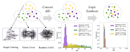
Existing learning based SAT solvers [9, 7, 6, 8] show poor generalization ability for different SAT classes, i.e., they need to design different heuristics for different distributions of SAT problems. Figure 1 shows the distribution diversity among three SAT instances, each belonging to a different SAT class. [7] also observe that the performance of heuristic specialized to a particular SAT distribution degrades considerably on other distributions.
To this end, we leverage the logic synthesis techniques [13, 14] in the EDA field to reduce the distribution diversity among different SAT distributions, thus improving the generalizability of DeepSAT. Specifically, we first represent the given SAT instances in AIG format. Then we apply two logic synthesis techniques, i.e., logic rewriting [14] and logic balancing [21]. The former reduces the total number of AIG nodes, and latter constructs a more balanced circuit with minimal logic level. Please refer to [22] for more technical details about these techniques.
We quantitatively show the change of the distributions before and after logical synthesis, using a scale-independent measurement, i.e., balance ratio (BR) [23] - the average ratio of larger fanin region size to smaller fanin region size for each two-fanin gate, i.e., AND gate in AIG. A BR value closer to 1 indicates more balanced fanin regions of the gate. As shown in Figure 1, AIGs from different SAT sources have distinct frequency histogram of BR values. But after performing logic synthesis, these histograms become similar showing BR values close to 1, since all the AIGs are optimized to have more balanced fanin regions of the gate. This demonstrates that logic synthesis can reduce the distribution diversities among AIGs from different SAT sources, which naturally introduces a strong inductive bias (i.e., compactness and balance) for more effective SAT solving.
III-C SAT Solving as a Conditional Generative Procedure
Problem formulation. As introduced in Section III-A, we represent a Boolean formula as an AIG-based directed graph , where the nodes correspond to the primary inputs (PIs), the nodes denote the logic gates, and the directed edges represent wires among the gates. The PI states can be viewed as a random variable following the multivariate Bernoulli distribution, , where is the number of PIs and is the parameter of the distribution. The primary output (PO) is the state of the gate at the last logic level, which follows the univariate Bernoulli distribution, indicating whether the Boolean circuit evaluates to logic ‘1’ or not. A feasible solution for a satisfiable Boolean circuit can be derived by:
| (1) |
Similar to PixelCNN [15], we handle the intractable joint probability distribution of by factorizing it into a product of conditional univariate Bernoulli distributions:
| (2) |
where denote the PIs of which the values have been determined, and .
Supervision label construction. To obtain the joint probability in Equation 2, we need to figure out , and then calculate . Note that different from PixelCNN [15], we do not have a natural fixed order for picking s. To facilitate subsequent discussions, we rewrite the condition terms in Equation 2 as . The determined PIs are designated using a mask to simulate the generative procedure, which is applied on all nodes to indicate whether the state of a node is determined or not:
| (3) |
Following a frequentest setting, we estimate a value for each by maximum likelihood estimation (MLE). Suppose we feed random assignments (also known as logic simulation in EDA context) to the Boolean circuit and observe variable being logic ‘1’ for times. Then we can obtain the maximum likelihood estimator for of :
| (4) |
It should be noted that such estimation is achieved without any conditions, e.g., the circuit being satisfiable or values of some nodes are known in advance. If some conditions are imposed into the circuit, we simply filter out the random assignments that violate the conditions during logic simulation, therefore can estimate in the conditional distribution.
We refer as the simulated probability of node being logic ‘1’ in the following discussion. To avoid in-accurate estimation associated with maximum likelihood, we perform logic simulations with a large number of random patterns (e.g., k random patterns to each AIG in our experiments) to obtain faithfully simulated probability values. Alternatively, for larger problems, a practical way is to first use an efficient all solutions SAT solver [24] to obtain all possible satisfying solutions, and then estimate the supervision signal from these assignments. In general, the cost of our logic simulation is on par with those of other SAT solving algorithms such as NeuroSAT [9], where the SAT-related supervision labels are generated from a classical SAT solver.
Training objective. The core of our approach is a graph-based model taking a DAG and the conditions as inputs to approximate the simulated probabilities at the node-level directly. Our hypothesis is that a DAG structure sufficiently defines the logic computation of the Boolean circuit and characterizes the dependence of the different gates/variables. With enough relational inductive biases, a parameterized graph-based model is able to predict the simulated probability of all gates under logic simulation. Driven by this hypothesis, we designate the training objective as the following mapping:
| (5) |
where the condition corresponds to the determined nodes defined by the mask (Equation 3). We generate a mask initialized from a zero vector by fixing the element for PO to 1 (i.e., let ), and then assign the elements corresponds to a randomly designated condition terms with 1 or -1. Given , the objective is to regress the simulated probabilities of the remaining nodes being logic ‘1’, i.e., to approximate . Each conditional probability is parameterized by a deep neural network whose architecture is chosen according to the required inductive biases for the graph-structured Boolean circuits. The function is learned by minimizing the least absolute error between the prediction and the supervision label .
III-D The Proposed Model
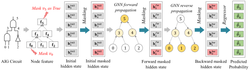
To capture directed relational bias embedded in circuits, we leverage the dedicated directed acyclic GNNs (DAGNNs) [19] as the model in Equation 5 to learn structural information and the computational behavior of logic circuits, and embed them as vectors on every logic gate [20]. As shown in Figure 2, the model consists of two stages of directed acyclic GNN propagation along with the masking operations defined in Equation 3. Then a multi-layer perceptron (MLP) regressor is applied on node vectors for predicting the simulated probability.
Given a circuit graph , we use and to denote the gate type and the hidden vector, respectively. Specifically, as three types of gates, i.e., PI, AND and NOT, are present in AIGs, we encode the gate type as a -d one-hot embedding for each node according to its gate type. We elaborate the details of the model design in DeepSAT below.
Polarity prototypes. The training objective derived in Equation 5 requires the model to be able to condition on some given gate states. To enable such conditional modeling, we define two prototypes [25], and , for two polarities of node probabilities, one for node being logic ‘1’ (positive polar) and the other for node being logic ‘0’ (negative polar), respectively.
Assuming every node is encoded as a hidden vector , the hidden vectors for the masked nodes are replaced by their corresponding prototypes according to the value of the mask:
| (6) |
In practice, the initial hidden vectors are sampled from a normal Gaussian distribution. Therefore, we fix the hidden vectors for two polarities as two near-boundary points, i.e, all positive ones for logic () and all negative ones for logic (), respectively. The two polarity prototypes can be thought of as two extreme points lying on opposite sides of a sphere in hidden space. Intuitively, during training, the hidden vectors of gates with a probability close to will be pulled to all ones, and vice versa. Therefore, the two polarity prototypes facilitate learning a continuous and compact hidden space with good interpretability of logic values. Note that other polarity prototypes are also feasible, as long as the two polarity prototypes are far away from each other in the hidden space.
For notational simplicity, we omit the superscript prime ’′’, and directly use to denote the input hidden vector after the masking operation defined in Equation 6.
Forward propagation. To aggregate the information from node ’s predecessors, we implement the attention mechanism in the additive form [19] as:
| (7) |
where denotes the set of direct predecessors of . Using the ‘Attention’ language, the inital hidden state serves as a query, and the representation of predecessors serves as a key. We then use the Gated Recurrent Unit (GRU) to combine the aggregated information with ’s information, including the encoded gate type and the initial hidden vector to update the hidden vector of target node :
| (8) |
wherein , are concatenated together and treated as input, while is the past state of GRU. The above functions process nodes according to the logic levels defined by circuit’s topological orders, starting from PIs and ending up with the single PO. After that, the node hidden vector is further updated by according to the same mask following Equation 6.
Reverse propagation. To model the effect of the conditional term related to satisfiability, i.e., in Equation 5, we perform a reverse information propagation after the forward propagation. Specifically, we impose the condition of satisfiability PO by masking its hidden vector as , and process the graph in reversed topological order to propagate the condition to PIs. By doing so, the updated node hidden vector contains extra information about the satisfiability compared with that is obtained only using forward propagation.
The backward propagation is similar to the forward propagation regarding computation of aggregation and combination function, except that during the aggregation, we only consider the direct successors of target node . The hidden vector is further processed using the same mask as above following Equation 6, and fed into the regressor for predicting the simulated probabilities.

Comparison with previous methods using bidirectional propagation. Adopting a reverse propagation besides the forward propagation for training DAG structures is not new in GNN-based SAT solving [10, 19], yet we highlight key differences that support the superior SAT solving performance of DeepSAT. In DAGNN [19] and DG-DAGRNN [10], the reason to perform forward and reverse propagation is to enrich the node state vectors with information from both the ancestor and the descendant nodes. While in DeepSAT, the goal of using bidirectional propagation along with polarity prototypes is to mimic the Boolean constraint propagation (BCP) [26, 27] mechanism in logic reasoning.
Specifically, BCP is initiated when a logic value is assigned to an unassigned gate , which leads to value changing of some unassigned gates in the neighbourhood of (i.e., fanin and fanout). There are two types of propagation considering the direction: forward propagation and reverse propagation (Figure 3). Similarly, in DeepSAT, we introduce polarity prototypes as hidden states for gates assigned with known logic states. Specially, the satisfiability is modeled by assigning logic ‘1’ to PO. To this end, optimizing the conditional gate-level probability (Equation 2) with bidirectional propagation and polarity prototypes enables learning BCP in the hidden space (Figure 3). Such design encourages a continuous and compact hidden space with good interpretability of logic values. More importantly, with polarity-regularized hidden space, we can manipulate the states of nodes and thus perform conditional solution sampling as described below.
III-E Solution sampling scheme
To sample solutions from the well-trained conditional model, we iteratively select the undetermined PI with the highest confidence values predicted by the model, i.e., the PI with probability prediction closest to or . Specifically, given an SAT instance with variables, we conduct the following auto-regressive procedure: 1) We mask PO as logic ‘1’, and generate the corresponding mask vector . 2) At iteration , we pass to well-trained DeepSAT model to estimate the simulated probability of all un-masked PIs. The PI with the highest confidence is selected and masked as logic ‘0’ if the prediction is smaller than 0.5, otherwise logic ‘1’. According to the selected PI and its masked value, a new mask is generated. 3) Repeat the second step until all PIs have been masked ( iterations in total). Then we obtain a candidate assignments from .
To explore more possible assignments to satisfy the SAT instance, we also develop a simple flipping-based strategy to sample more solutions from the conditional model ( solutions in the worst case). Briefly, if the initial sampled assignment is not the satisfying solution, we record the order of PIs being masked and flip a specific PI in the next sampling step, following the recorded order.
IV Experiments
| Same Iterations | Test Metric Converges | |||||||||||
| Methods | Format | SR() | SR() | SR() | SR() | SR() | SR() | SR() | SR() | SR() | SR() | |
| NeuroSAT | CNF | 65% | 58% | 32% | 20% | 20% | 92% | 74% | 42% | 20% | 20% | |
| DeepSAT | Raw AIG | 67% | 60% | 36% | 23% | 21% | 94% | 79% | 45% | 25% | 23% | |
| Opt. AIG | 72% | 66% | 40% | 31% | 23% | 98% | 85% | 51% | 37% | 26% | ||
IV-A Experimental settings
Baselines. We compare our solution with the representative end-to-end method for SAT solving in the literature 111We do not compare DeepSAT with DG-DAGRNN [10] as we cannot reproduce its results, despite that we have rigorously followed the descriptions in the paper.: NeuroSAT [9]. NeuroSAT assumes that the input problem is in CNF. There are several follow-up works of NeuroSAT [7, 6, 8, 11] that consuming CNFs. Nevertheless, they target on different settings and NeuroSAT still stands for a strong baseline for end-to-end SAT solving. To enable a fair comparison, we implement DeepSAT and NeuroSAT in a unified frameworkwith PyTorch Geometric (PyG) [28] package.
Training datasets. We follow the SAT instance generation scheme proposed in NeuroSAT [9] to generative random -SAT CNF pairs. We use SR() to denote random -SAT problems on variables generated by this scheme. In particular, we generate a SR() dataset of k SAT and UNSAT pairs. We restrict the scale of the training dataset due to limited GPU resources. However, we demonstrate that DeepSAT can generalize well to problems that are larger or with novel distributions, as shown below. For NeuroSAT, these pairs are directly used for binary classification, while DeepSAT is only trained on SAT instances. For DeepSAT, we convert CNFs to Raw AIG222Convert CNF to AIG using the cnf2aig tool: http://fmv.jku.at/cnf2aig/and Optimized AIG via logic synthesis (abbreviated as Opt. AIG). Note that in all experiments we convert the test instances to the same formats as the ones used in model training.
Evaluation metric. DeepSAT is an incomplete [8, 10] solver, i.e., an instance is detected as satisfiable only after the model finds a satisfying assignment and otherwise returns unsolved. Therefore, we only include satisfiable instances in the testing dataset for all experiments and measure the percentage of the successfully solved SAT instances out of all instances (abbreviated as Problems Solved).
IV-B Random k-SAT
This section shows comparisons of DeepSAT and NeuroSAT on solving random -SAT problem. To evaluate the generalization performance, we validate our method on SAT instances generated from a much larger number of variables. In particular, we evaluate the well-trained DeepSAT on SR(), SR(), SR(), SR() and SR(), and compare with the results with the baseline.
Since DeepSAT and NeuroSAT use different assignment decoding schemes to yield the SAT assignments given an SAT instance, we consider two experimental settings for performance comparison: i) compare under the same computational cost, which is measured by the number of message passing iterations, and ii) compare the upper-bound of performance regardless of the computational cost. For the first setting, we fix the number of message passing iterations as for an -variable SAT instance. This is because DeepSAT needs to perform at least message passing iterations to generate a solution for an -variable SAT instance, while NeuroSAT can generate the solution for a specific problem once by clustering on the literal embedding after a number of bidirectional message passing iterations. Hence, for a -variable SAT instance, we fix the number of message passing iterations as , in which case DeepSAT can generate one and only one complete assignment and NeuroSAT are aligned with same message passing cost. For the second setting, we let both models generate as many assignments as possible until the test metric converges. In this way, NeuroSAT is queried for multiple times for assignment decoding under different iterations of message passing, in order to monitor the test metric. In other words, NeuroSAT will generate multiple assignments for one SAT instance. As for DeepSAT, we follow the proposed solution sampling scheme introduced in Section III-E, which samples at most solutions in worst case.
We present Problems Solved on different testing datasets with different formats in Table I. From this table, we have several observations. First, compared with the baselines, DeepSAT can achieve the highest Problems Solved on all evaluated datasets under both experiment settings, with a significant margin. For example, on SR(), DeepSAT trained on Opt. AIGs can solve of problems, while NeuroSAT trained on CNFs only solve of problems. Second, the performance of both models degrades as we increase the number of variables. Yet, DeepSAT generalizes better to bigger and harder problems than NeuroSAT.
To further validate the effectiveness of our proposed formulation, i.e., SAT solving as a generative modeling procedure, we monitor Problems Solved during the solution sampling procedure on SR(). By sampling a single solution for each problem, DeepSAT can solve of all problems. If we sample two more solutions for each problem from DeepSAT, the percentage of solved problems increases to . Contrarily, to solve of problems on SR(), NeuroSAT requires additional tens of iterations of message propagation to make prediction coverage. DeepSAT terminates when the latest sampled solutions are satisfying and samples solutions on average for SR(). The result on other test datasets shows the same tendency.
IV-C Effectiveness of Logic Synthesis
In Table I, we see that DeepSAT maintains state-of-the-art performance even when trained on raw AIGs without logic synthesis. Specifically, DeepSAT trained on raw AIGs outperforms NeuroSAT trained on CNFs consistently across all test sets, despite that raw AIGs include less structural information for learning. For example, DeepSAT trained on raw AIGs successfully solves and out of SR() and SR() problems, respectively, which is better NeuroSAT trained on CNFs. In summary, we believe that the performance gain of DeepSAT not only comes from EDA optimization, but also thanks to the customized bidirectional propagation with polarity prototypes that can effectively model the conditional distribution of possible assignments.
| Method | Format | Coloring Acc. | Domset Acc. | Clique Acc. | Vertex Acc. | Avg. Acc. |
|---|---|---|---|---|---|---|
| NeuroSAT | CNF | 0% | 44% | 35% | 0% | 22% |
| DeepSAT | Raw AIG | 63% | 81% | 77% | 82% | 76% |
| Opt. AIG | 98% | 99% | 92% | 97% | 97% |
IV-D Novel Distributions
To further investigate the generalization ability of our DeepSAT model, we evaluate the model trained on SR() on the different NP-Complete problems with novel distributions: graph -coloring, vertex -cover, -clique-detection and dominating -set. The above problems can be reduced to the SAT problems and solved by a SAT solver. We generate 100 random graphs with nodes and the edge percentage of for each problem. For each graph in each problem type, we generate graph coloring instances (), dominating set problems (), clique-detection problems () and vertex cover problems (). We report the results when the test metric converges. Notably, the generated problem instances are not particularly difficult for state-of-the-art SAT solvers. For our purpose, the evaluated results in this section serve as simple benchmarks to demonstrate the superiority of DeepSAT over the baseline.
As shown in Table II, DeepSAT trained on Opt. AIGs can solve of graph coloring problems, of dominating set problems, of clique-detection problems, and of vertex cover problems. When DeepSAT is trained on raw AIGs, the performance degrades to some extent, yet is still better than NeuroSAT on these datasets. In contrast, we observe there is an apparent discrepancy in performance of NeuroSAT between novel distribution problems and the in-sample distribution used for training, even though the size of problems is similar. To sum up, DeepSAT maintains the same solving ability on novel problems, and the pre-processing of logic synthesis enables better generalization ability of novel distributions.
V Conclusion and Future Work
This paper presents DeepSAT, an EDA-driven end-to-end learning framework for SAT solving. Specifically, we first propose to apply a logic synthesis-based pre-processing procedure to reduce the distribution diversity among various SAT instances. Next, we formulate SAT solving as a conditional generative procedure and construct more informative supervisions with simulated logic probabilities. A dedicated directed acyclic graph neural network with polarity prototypes is then trained to approximate the conditional distribution of SAT solutions. Our experimental results show that DeepSAT outperforms the existing end-to-end baseline.
While DeepSAT demonstrates considerable improvements in end-to-end SAT solving, there is still a significant performance gap compared to state-of-the-art heuristic-based SAT solvers. In our future work, on the one hand, we plan to improve its performance further; on the other hand, we would also explore novel joint solutions that combine them, e.g., using constraint propagation mechanism learned in DeepSAT to guide better heuristic in classical Circuit-SAT solvers.
References
- [1] M. Büttner and J. Rintanen, “Satisfiability planning with constraints on the number of actions.” in International Conference on Automated Planning and Scheduling, 2005, pp. 292–299.
- [2] A. Horbach, “A boolean satisfiability approach to the resource-constrained project scheduling problem,” Annals of Operations Research, vol. 181, no. 1, pp. 89–107, 2010.
- [3] Y. Vizel, G. Weissenbacher, and S. Malik, “Boolean satisfiability solvers and their applications in model checking,” Proceedings of the IEEE, vol. 103, no. 11, pp. 2021–2035, 2015.
- [4] N. Sorensson and N. Een, “Minisat v1. 13-a sat solver with conflict-clause minimization,” SAT, vol. 2005, no. 53, pp. 1–2, 2005.
- [5] A. B. K. F. M. Fleury and M. Heisinger, “Cadical, kissat, paracooba, plingeling and treengeling entering the sat competition 2020,” SAT COMPETITION, vol. 2020, p. 50, 2020.
- [6] V. Kurin, S. Godil, S. Whiteson, and B. Catanzaro, “Can q-learning with graph networks learn a generalizable branching heuristic for a sat solver?” Advances in Neural Information Processing Systems, vol. 33, pp. 9608–9621, 2020.
- [7] E. Yolcu and B. Póczos, “Learning local search heuristics for boolean satisfiability,” Advances in Neural Information Processing Systems, vol. 32, 2019.
- [8] W. Zhang, Z. Sun, Q. Zhu, G. Li, S. Cai, Y. Xiong, and L. Zhang, “Nlocalsat: boosting local search with solution prediction,” in Proceedings of the Twenty-Ninth International Conference on International Joint Conferences on Artificial Intelligence, 2021, pp. 1177–1183.
- [9] D. Selsam, M. Lamm, B. Bünz, P. Liang, L. de Moura, and D. L. Dill, “Learning a SAT solver from single-bit supervision,” in International Conference on Learning Representations, 2019.
- [10] S. Amizadeh, S. Matusevych, and M. Weimer, “Learning to solve circuit-SAT: An unsupervised differentiable approach,” in International Conference on Learning Representations, 2019.
- [11] H. Duan, P. Vaezipoor, M. B. Paulus, Y. Ruan, and C. Maddison, “Augment with care: Contrastive learning for combinatorial problems,” in International Conference on Machine Learning. PMLR, 2022, pp. 5627–5642.
- [12] C.-A. Wu, T.-H. Lin, C.-C. Lee, and C.-Y. Huang, “Qutesat: a robust circuit-based sat solver for complex circuit structure,” in 2007 Design, Automation & Test in Europe Conference & Exhibition. IEEE, 2007, pp. 1–6.
- [13] P. Bjesse and A. Boralv, “Dag-aware circuit compression for formal verification,” in IEEE/ACM International Conference on Computer Aided Design, 2004. ICCAD-2004. IEEE, 2004, pp. 42–49.
- [14] A. Mishchenko, S. Chatterjee, and R. Brayton, “Dag-aware aig rewriting: A fresh look at combinational logic synthesis,” in 2006 43rd ACM/IEEE Design Automation Conference. IEEE, 2006, pp. 532–535.
- [15] A. v. d. Oord, N. Kalchbrenner, O. Vinyals, L. Espeholt, A. Graves, and K. Kavukcuoglu, “Conditional image generation with pixelcnn decoders,” in Proceedings of the 30th International Conference on Neural Information Processing Systems, 2016, pp. 4797–4805.
- [16] E. Khalil, H. Dai, Y. Zhang, B. Dilkina, and L. Song, “Learning combinatorial optimization algorithms over graphs,” Advances in neural information processing systems, vol. 30, 2017.
- [17] B. Hudson, Q. Li, M. Malencia, and A. Prorok, “Graph neural network guided local search for the traveling salesperson problem,” in International Conference on Learning Representations, 2022.
- [18] Z. Wu, S. Pan, F. Chen, G. Long, C. Zhang, and S. Y. Philip, “A comprehensive survey on graph neural networks,” IEEE transactions on neural networks and learning systems, vol. 32, no. 1, pp. 4–24, 2020.
- [19] V. Thost and J. Chen, “Directed acyclic graph neural networks,” in International Conference on Learning Representations, 2021.
- [20] M. Li, S. Khan, Z. Shi, N. Wang, Y. Huang, and Q. Xu, “Deepgate: learning neural representations of logic gates,” in Proceedings of the 59th ACM/IEEE Design Automation Conference, 2022, pp. 667–672.
- [21] J. Cortadella, “Timing-driven logic bi-decomposition,” IEEE Transactions on Computer-Aided Design of Integrated Circuits and Systems, vol. 22, no. 6, pp. 675–685, 2003.
- [22] R. Brayton and A. Mishchenko, “Abc: An academic industrial-strength verification tool,” in International Conference on Computer Aided Verification. Springer, 2010, pp. 24–40.
- [23] A. Walker and D. Wood, “Locally balanced binary trees,” The Computer Journal, vol. 19, no. 4, pp. 322–325, 1976.
- [24] T. Toda and T. Soh, “Implementing efficient all solutions sat solvers,” Journal of Experimental Algorithmics (JEA), vol. 21, pp. 1–44, 2016.
- [25] J. Snell, K. Swersky, and R. Zemel, “Prototypical networks for few-shot learning,” in Proceedings of the 31st International Conference on Neural Information Processing Systems, 2017, pp. 4080–4090.
- [26] A. Belov and Z. Stachniak, “Improved local search for circuit satisfiability,” in International Conference on Theory and Applications of Satisfiability Testing. Springer, 2010, pp. 293–299.
- [27] H.-T. Zhang, J.-H. R. Jiang, and A. Mishchenko, “A circuit-based sat solver for logic synthesis,” in 2021 IEEE/ACM International Conference On Computer Aided Design (ICCAD). IEEE, 2021, pp. 1–6.
- [28] M. Fey and J. E. Lenssen, “Fast graph representation learning with PyTorch Geometric,” in ICLR Workshop on Representation Learning on Graphs and Manifolds, 2019.