Observable effect of quantized cylindrical gravitational waves

Abstract

We investigate the response of a model gravitational wave detector consisting of two particles to the quantized cylindrical gravitational waves and obtain a relation between the standard deviation of the distance between two particles and the distance from the source to the detector. It is found that the quantum effect carried by the cylindrical gravitational wave can be observed above Planck scale even though the source is as far as the cosmological horizon. The equation of motion for the change of the distance between two particles is obtained when the cylindrical gravitational waves pass. It is surprising that the dissipative term does not exist up to the first order approximation due to cylindrical symmetry of the gravitational wave.

I Introduction

Some physical effects such as black hole evaporation and early-universe cosmology ck07 ; cr08 imply there should be a quantum theory about gravity, but there is no experimental or observational evidence to support that ck06 ; arp14 ; adm14 up to now. An important confirmation is to test the hypothetical quanta of the gravitational field such as gravitons, but it is nearly impossible to conclude in the foreseeable future fd13 ; kst21 . Gravitational waves (GWs), however, can be used to examine the possible implications for the quantization of gravity since the GWs have been directly detected by LIGO in 2015 for the first time aaa16 .

Recently, Parikh, Wilczek and Zahariade treated the GWs as quantum entity and explored its implications for quantization of gravity from the perspective of experimental observation pwz211 ; pwz212 . They calculated the effect of quantized gravitational field on falling bodies, and found that the dynamics of the separation of a pair of free falling particles is no longer deterministic, but probabilistic, as acted on by a novel stochastic force. In this paper, we will investigate this using the Einstein-Rosen wave er37 by coupling it with a pair of free falling particles which is a simplified model for the GW detector.

The Einstein-Rosen wave is an exact solution of general relativity with two commuting Killing vectors and describes a cylindrical GW, so using it to study the aspects of nonlinearity originating from Einstein gravity is convenient and significant mt17 . Historically, it played an important role in early attempts at defining the energy carried by gravitational waves kst65 ; sc86 , since the energy of GWs is difficult to be described locally due to the equivalence principle rai68 ; mab97 ; fjb40 ; llf75 . Thus, the Einstein-Rosen waves as cylindrical GWs from some proper astrophysical sources bsw20 could be observed really ww57 as they can carry the energy with themselves. Moreover, the Einstein-Rosen wave has a nice quantum description kk71 and its quantization coupled to massless scalar field has been obtained gv05 . Although the quantization of Einstein-Rosen cylindrical GWs has received a lot of attention aa96 ; ap96 ; am00 ; gp97 ; dt99 ; mv00 ; cms98 ; rt96 ; ks98 ; bgv03 ; bgv04 , its implication from the observable point of view has not been discussed. In this paper, we study its possible quantum signatures from cylindrical GWs by calculating the response of a model GW detector to the quantized gravitational field. It is found that the signatures for the quantization of GWs contains the information about the distance from the source to the detector which is derived from the specific form of cylindrical GWs and cannot be obtained from the general description for GWs.

The paper is organized as follows. In the second section, the theory of Einstein-Rosen wave is reviewed. In particular, its quantized form is given for the later discussion for the observable effect of cylindrical GWs. In the third section, we use a simple detection model to study the observable effect of the cylindrical GWs and some novel results are obtained. Finally, we give a conclusion in the fourth section.

II Einstein-Rosen wave

Consider a spacetime with the cylindrical symmetry and its metric can be expressed with a conformally flat form kk71 ,

$$ds^{2}=e^{-\psi}\left[e^{\gamma}\left(-dT^{2}+dR^{2}\right)+R^{2}d\theta^{2}\right]+e^{\psi}dZ^{2},$$ (1)

where the metric functions $\psi$ and $\gamma\$depend only on the coordinates $R$ and $T$. Using the vacuum Einstein field equation, it is obtained that

$$\frac{\partial^{2}\psi}{\partial T^{2}}-\frac{\partial^{2}\psi}{\partial R^{2}}-\frac{1}{R}\frac{\partial\psi}{\partial R}=0,$$ (2)

which is the wave equation of physical degrees of freedom and has exactly the same form as the wave equation of the cylindrically symmetric massless scalar field $\psi$ evolving in Minkowskian spacetime background kk71 . This means that the metric function $\psi$ represents cylindrical gravitational waves or Einstein-Rosen waves. The metric function $\gamma$ can be obtained as

$$\gamma=\frac{1}{2}\int_{0}^{R_{0}}dRR\left[\left(\frac{\partial\psi}{\partial T}\right)^{2}+\left(\frac{\partial\psi}{\partial R}\right)^{2}\right].$$ (3)

This is the energy of cylindrical GWs in a ball of radius $R_{0}$, which derives from the definition about C-energy introduced by Thorne kst65 and a recent detailed discussion refers to Ref. bgp19 .

The solution of Eq. (2) for a particular wave number $k$ can be obtained as

$$\psi_{k}(R,T)=\frac{1}{\sqrt{2\hbar G}}J_{0}(kR)\left(a(k)e^{-ikT}+a^{\dagger}(k)e^{ikT}\right),$$ (4)

where $J_{0}(kR)$ is the Bessel function of zeroth order. When the canonical quantization is implemented, the parameters $a(k)$ and $a^{\dagger}(k)$ are regarded as operators satisfying the commutation relations $\left[a(k),a^{\dagger}(k^{\prime})\right]=\hbar\delta(k,k^{\prime})$, and they can be physically interpreted as annihilation and creation operators.

As discussed in the Introduction, the observable effect of cylindrical GWs is considered at the place with a large distance from the source, so the linearized form of this metric (1),

$$ds^{2}=(1-\psi)ds_{3}^{2}+(1+\psi)dZ^{2},$$ (5)

with $ds_{3}^{2}=-(1+\gamma)dT^{2}+(1+\gamma)dR^{2}+R^{2}d\theta^{2}$, is adequate in the following discussion. It is noted that in the linearized metric, the wave equation (2) still holds, but the energy function $\gamma$ takes the asymptotic form. When $R\ \rightarrow\infty$, the energy of gravitational waves is obtained as

$$\gamma_{\infty}=\int_{0}^{\infty}dkka^{\dagger}(k)a(k),$$ (6)

by putting the Eq. (4) into Eq. (3) and taking the large $R$ limit ap96 ; bgv03 . This shows that the energy remains finite at large $R$.

According to the analyses in Refs. kk71 ; rt96 ; bgv03 , the Hamiltonian of this linearized gravity can be written as

$$H_{G0}=\int_{0}^{\infty}dR\left[\frac{p_{\psi}^{2}}{2R}+\frac{R}{2}\left(\frac{\partial\psi}{\partial R}\right)^{2}\right],$$ (7)

where the gauge fixing conditions $p_{\gamma}=0$ and $R=r$ are imposed. $p_{\psi}$ and $p_{\gamma}$ are the canonical momenta conjugated to the metric fields $\psi$ and $\gamma$, respectively. $R=r$ indicates that $R$ can be used to measure the distance from the source to the detector. Noted that the metric in Eq. (1) has used the gauge $R=r$ since in the initial expression the term $R^{2}d\theta^{2}$ should be $r^{2}d\theta^{2}$. It is not hard to confirm that $H_{G0}=\gamma_{\infty}$ when the expression of $p_{\psi}$ is used. For the cylindrical GWs, there is another physically related Hamiltonian $H_{G}=2\left(1-e^{-H_{G0}/2}\right)$ which describes the energy per unit length along the symmetry axis in general relativity ap96 . $H_{G}$ is related to the physical time $t$ which is gotten by the transformation $t=e^{\gamma_{\infty}/2}T$. Furthermore, with time $t$, the annihilation and creation operators can expressed as

$$a_{E}(k,t) =a(k)\exp\left[-itE(k)e^{-H_{G0}/2}\right],$$

$$a_{E}^{\dagger}(k,t) =a^{\dagger}(k)\exp\left[itE(k)e^{-H_{G0}/2}\right],$$ (8)

where $E(x)=2\left(1-e^{-x/2}\right)$. When the dimensional constants $\hbar$ and $G$ are restored, $E(k)$ can be expressed as $\left(1-e^{-4\hbar G}\right)/(4G)$, which gives $\frac{1}{\hbar}E(k)=k+O\left(\hbar\right)$. Thus, we take the first approximation $E(k)\sim k$ in the calculation below. Substituting these equations into metric field in Eq. (4), we have

$$\psi(R,t)=\frac{1}{\sqrt{2\hbar G}}\int_{0}^{\infty}dkJ_{0}(kR)\left[a_{E}(k,t)+a_{E}^{\dagger}(k,t)\right].$$ (9)

Define $q_{k}(t)=a_{E}(k,t)+a_{E}^{\dagger}(k,t)$, and decompose $\psi(R,t)$ into discrete modes. Thus, the metric field becomes

$$\psi(R,t)=\frac{1}{\sqrt{2\hbar G}}\sum_{k}J_{0}(kR)q_{k}(t),$$ (10)

where the zeroth-order Bessel function $J_{0}(kR)$ satisfies the integral relation, $\int_{0}^{\infty}dRRJ_{0}(kR)J_{0}(k^{\prime}R)=\frac{L}{2\pi}\delta(k-k^{\prime})$, for the period boundary condition $k=2\pi R/L$.

Based on the discussion above, the Einstein-Hilbert action of linearized cylindrically symmetric GWs can be written as

$$S_{G} =\frac{1}{64\pi G}\int_{t_{1}}^{t_{2}}\int_{0}^{\infty}dTdR\left(p_{\psi}\frac{\partial\psi}{\partial T}-H_{0}\right)$$

$$=\frac{1}{64\pi G}\int_{t_{1}}^{t_{2}}\int_{0}^{\infty}dTdR\frac{R}{2}\left[\left(\frac{\partial\psi}{\partial T}\right)^{2}-\left(\frac{\partial\psi}{\partial R}\right)^{2}\right]$$

$$=\frac{1}{2}m\int_{t_{1}}^{t_{2}}dt\sum_{k}\left((\dot{q}_{k})^{2}-e^{-\gamma_{\infty}}k^{2}(q_{k})^{2}\right),$$ (11)

where the dot denotes the derivative with respect to $t$. $m\equiv\frac{e^{\frac{\gamma_{\infty}}{2}}L}{128\pi^{2}\hbar G^{2}}$ is similar to the meaning of the mass, $p_{\psi}=R\frac{\partial\psi}{\partial T}$ is used in the second line, and Eq. (10) and the integral relation for the zeroth-order Bessel function $J_{0}(kR)$ are used in the third line.

III Detection

In this section, we consider the observable effect of the cylindrical GWs. In this linearized metric (5), the Riemann curvature tensor $R_{\text{ }0,R0}^{R}$ can be calculated, which gives the geodesic deviation equation, $\frac{d^{2}l}{dt^{2}}=-R_{\text{ }0,R0}^{R}l$ with $l$ denoting the distance between two free falling testing particles. With these, we can construct a simple model to test the cylindrical GWs by the change of the distance between a pair of particles with the action,

$$S_{M} =\int_{t_{1}}^{t_{2}}dt\left(\frac{1}{2}m_{0}\dot{l}^{2}-\frac{1}{2}m_{0}\left(\dot{\gamma}-\dot{\psi}\right)\dot{l}l\right)$$

$$=\int_{t_{1}}^{t_{2}}dt\left(\frac{1}{2}m_{0}\dot{l}^{2}+g\sum_{k}J_{0}(kR)\dot{q}_{k}\dot{l}l\right),$$ (12)

where $m_{0}$ is the mass of the particle and $g\equiv\frac{m_{0}}{2\sqrt{2\hbar G}}$ similar to the coupling parameter between the GWs and two particles. In the second line of the calculation, Eq. (10) is used, and $\dot{\gamma}=0$ is imposed when the distance $R$ is large as required for the discussion of the observable effect of cylindrical GWs. The independence of $\gamma$ on the time means that the energy carried by the cylindrical GWs is constant at large $R$ gv05 ; ap96 ; bgv03 . Thus, the effect of the cylindrical GWs on the distance between two particles derives mainly from the metric function $\psi$.

Together with the action of cylindrical GWs, we have the total action as

$$S=S_{G}+S_{M}.$$ (13)

Now we can calculate the physical effect. Similar to the consideration in Refs. pwz211 ; pwz212 , the transition probability of the particles from the state $\phi_{A}$ to state $\phi_{B}$ in time $t$, $P_{\psi_{\omega}}(\phi_{A}\rightarrow\phi_{B})=\sum_{\left|f\right\rangle}|\left\langle f,\phi_{B}\right|U(t_{f},0)\left|\psi_{\omega},\phi_{A}\right\rangle|^{2}$ where $\psi_{\omega}$ and $f$ are the initial and final gravitational field states, is calculated in what follows. $U(t_{f},0)$ is the time evolving operator which is related to the total Hamiltonian of the combined GWs with particles. Due to the weak gravitational field, linearity allows us to write the whole action as $S=\sum_{\omega}S_{\omega}$ with

$$S_{\omega}=\int_{t_{1}}^{t_{2}}dt\left(\frac{1}{2}m\dot{q}^{2}+\frac{1}{2}m_{0}\dot{l}^{2}-\frac{1}{2}m\omega^{2}q^{2}e^{-\gamma_{\infty}}+gJ_{0}(\omega R)\dot{q}\dot{l}l\right),$$ (14)

where the relativistic dispersion relation $\omega=k$ is used and the subscript on $q_{k}$ is ignored for brevity. Then, the total canonical momenta are introduced as $p=m\dot{q}+gJ_{0}(kR)\dot{l}l$ for the field and $\pi=m_{0}\dot{l}+gJ_{0}(kR)\dot{q}l$ for the particle system, and the total Hamiltonian is obtained as

$$H=\left(\frac{p^{2}}{2m}+\frac{\pi^{2}}{2m_{0}}-\frac{gp\pi J_{0}l}{mm_{0}}\right)\left(1-\frac{g^{2}J_{0}^{2}l^{2}}{mm_{0}}\right)^{-1}+\frac{1}{2}m\omega^{2}q^{2}e^{-\gamma_{\infty}}.$$ (15)

Thus, the time evolving operator can be calculated according to $U_{l}(t_{f},0)=\exp\left(-\frac{i}{\hbar}\int Hdt\right)$.

Inserting several complete bases of joint position eigenstates, $\int dqdl\left|q,l\right\rangle\left\langle q,l\right|$, and calculating the integral of the variables $q$ and $\pi$, the transition probability becomes

$$P_{\psi_{\omega}}[\phi_{A}\rightarrow\phi_{B}]=C\int\tilde{\mathcal{D}}l\tilde{\mathcal{D}}l^{\prime}e^{\frac{i}{\hbar}\int_{0}^{t_{f}}dt\frac{1}{2}m_{0}(\dot{l}^{2}-\dot{l}^{\prime 2})}F_{\psi_{\omega}}[l,l^{\prime}],$$ (16)

where the unrelated factor $C=\int dl_{i}dl_{i}^{\prime}dl_{f}dl_{f}^{\prime}\phi_{A}^{\ast}(l_{i}^{\prime})\phi_{B}(l_{f}^{\prime})\phi_{B}^{\ast}(l_{f})\phi_{A}(l_{i})$. $F_{\psi_{\omega}}[l,l^{\prime}]=\left\langle\psi_{\omega}\right|U_{l^{\prime}}^{\dagger}(t_{f},0)U_{l}(t_{f},0)\left|\psi_{\omega}\right\rangle$ is the well-known Feynman-Vernon influence functional fv63 ; ch94 ; blh99 . A further calculation (see the appendix for the detail) gives

$$F_{\psi_{\omega}}[l,l^{\prime}]=F_{0\omega}[l,l^{\prime}]\left\langle\psi_{\omega}\right|e^{W^{\ast}a^{\dagger}}e^{-Wa}\left|\psi_{\omega}\right\rangle,$$ (17)

where

$$W\equiv\frac{ig}{\sqrt{8m\hbar\omega}}\int_{0}^{t_{f}}dt\left(X(t)-X^{\prime}(t)\right)J_{0}(\omega R)e^{-it\omega e^{-\gamma_{\infty}/2}},$$ (18)

and

$$F_{0\omega}[l,l^{\prime}] =\exp[-\frac{g^{2}}{8m\hbar\omega}\int_{0}^{t_{f}}\int_{0}^{t}dtdt^{\prime}J_{0}(\omega R_{1})J_{0}(\omega R_{2})$$

$$\times\left(X(t)-X^{\prime}(t)\right)\left(X(t^{\prime})e^{-i(t-t^{\prime})\omega}-X^{\prime}(t^{\prime})e^{i(t-t^{\prime})\omega}\right)],$$ (19)

with $X(t)\equiv\frac{d^{2}}{dt^{2}}l^{2}(t)$ and $X^{\prime}(t)\equiv\frac{d^{2}}{dt^{2}}l^{\prime 2}(t)$. Note that we consider the source and the two particles being in the same line. $R_{1}$ and $R_{2}$ are the distances between the source and the two particles respectively, with $R_{2}-R_{1}=l$ for the distance between two particles.

The calculation above is made only for a single mode, and sum up all these modes to derive the vacuum influence phase as

$$i\Phi_{0}[l,l^{\prime}]$$

$$=\sum_{k}i\Phi_{0\omega}[l,l^{\prime}]$$

$$=-\frac{4\pi m_{0}^{2}G}{\hbar}\int_{0}^{t_{f}}\int_{0}^{t}dtdt^{\prime}\int_{0}^{\infty}d\omega[\cos((t-t^{\prime})\omega)$$

$$\times J_{0}(\omega R_{1})J_{0}(\omega R_{2})\left(X(t)-X^{\prime}(t)\right)\left(X(t^{\prime})-X^{\prime}(t^{\prime})\right)]$$

$$+\frac{i4\pi m_{0}^{2}G}{\hbar}\int_{0}^{t_{f}}\int_{0}^{t}dtdt^{\prime}\int_{0}^{\infty}d\omega[\sin((t-t^{\prime})\omega)$$

$$\times J_{0}(\omega R_{1})J_{0}(\omega R_{2})\left(X(t)-X^{\prime}(t)\right)\left(X(t^{\prime})+X^{\prime}(t^{\prime})\right)],$$ (20)

where the relation $F_{0\omega}[l,l^{\prime}]=\exp[i\Phi_{0}[l,l^{\prime}]]$ is used. It is surprising that the second term is zero due to the relation $\int_{0}^{\infty}J_{\nu}(ax)J_{\nu}(bx)\sin(cx)=0$ for the situation with $Re[\nu]>-1$, $0<c<b-a$, and $0<a<b$. As discussed in Refs. pwz211 ; pwz212 , the second term in Eq. (20) is related to the dissipation during the interaction between the GW and the particles. So the dissipation is zero in the situation we discuss due to the cylindrical symmetry of GW. Actually, this term could exist when the $E(k)$ takes the higher-order term, but these terms are suppressed by the higher-order power of $\hbar$.

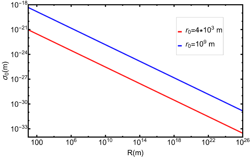
Figure 1: The standard deviation $\sigma_{0}$ for the change of the length between two particles (or test masses) influenced by cylindrical GWs as a function of the distance from the source to the detector. The length for different lines is taken according to the present setups or plans for GW detection, i.e. the red line represents the arm length of ground detector like LIGO and the blue line represents the arm length of spatial detectors like LISA, Taiji, or Tianqin.

Instead of continuing to calculate the transition probability that requires an unambiguous expression for the state $\left|\psi_{\omega}\right\rangle$ of the gravitational field, we use the correlation function to illustrate the observable effect. The correlation function can be defined as in pwz212 through the vacuum part of the influence phase by,

$$A_{0}(t,t^{\prime})\equiv\frac{4\hbar G}{\pi}\int_{0}^{\infty}d\omega\cos((t-t^{\prime})\omega)J_{0}(\omega R_{1})J_{0}(\omega R_{2}).$$ (21)

It is noted that $A_{0}(t,t^{\prime})=$ $\langle N_{0}(t)N_{0}(t^{\prime})\rangle=\int\mathcal{D}N_{0}\exp\left[-\frac{1}{2}\int_{0}^{T}\int_{0}^{T}dtdt^{\prime}A_{0}^{-1}(t,t^{\prime})N_{0}(t)N_{0}(t^{\prime})\right]N_{0}(t)N_{0}(t^{\prime})$ is the auto-correlation function of quantum stochastic noise $N_{0}$ using the Feynman-Vernon trick pwz212 ; fv63 . An observable signature is obtained through the standard deviation when $t^{\prime}=t$ given by

$$\sigma_{0} =\langle\left(l(t)-\langle l(t)\rangle\right)^{2}\rangle^{\frac{1}{2}}$$

$$\approx\frac{l_{0}}{2}\sqrt{\langle N_{0}(t)N_{0}(t)\rangle}$$

$$=\frac{l_{0}}{2}\sqrt{A_{0}(t,t)},$$ (22)

where $l_{0}$ is the initial distance between two particles (it can also be considered as the arm length of the GW detector hz22 ). $A_{0}(t,t)=\frac{4\hbar G}{\pi}\int_{0}^{\infty}d\omega J_{0}(\omega R_{1})J_{0}(\omega R_{2})$ is a convergent integral, which is different from the result in Refs. pwz211 ; pwz212 where the integral about $A_{0}(t,t)$ is divergent so the frequency has to be cut off at $\omega_{max}\sim$ $2\pi c/l_{0}$ with dipolelike approximation. A striking character of our result (22) is the dependence of the correlation function $A$ on the distance from the source to the detector. This is demonstrated in Fig. 1. It is seen that the samller the initial distance between two particles is, the higher the required sensitivity of detection would be. For the present detected possible sources that focused on the distance from the source to the detector about $1$ Gpc ($\sim 10^{25}m$) bpa1 ; bpa2 ; bpa3 , it is found that the present detector is unable to detect the quantum effect of GWs, since its requirement for the ability to detect the change of $10^{-32}$m for the length using the ground detector and $10^{-29}$m using the spatial detectors is beyond the ability of the present technology bbf16 ; pas12 ; jl16 ; hw17 . However, the quantum effect of cylindrical GW is larger than the Planck scale even though the distance from the source to the detector reaches at the cosmological horizon ($\sim 14$Gpc), which means that the quantum property of GW can be observed above Planck scale.

Finally, we want to give the expression for the equation of motion for the separation of two particles. For this, such term as $\left\langle\psi_{\omega}\right|e^{W^{\ast a\dagger}}e^{-Wa}\left|\psi_{\omega}\right\rangle$ in Eq. (17) has to be calculated. Using the same method as in Ref. pwz212 , we have the Langevin-like equation

$$\ddot{l}-\frac{1}{2}\left[\ddot{\psi}(t)+\ddot{N}_{0}(t)\right]l(t)=0,$$ (23)

for the state $\psi_{\omega}$ taken as the coherent state. The first term is related to the classical effect of cylindrical GW, and the second term derives from the quantum property of GW, which can be regarded as a stochastic noise pwz211 ; pwz212 distinguished from the classically deterministic evolution. In particular, the fifth-order derivative term that existed in the earlier discussion pwz211 ; pwz212 disappears here because the second term is zero in Eq. (20). Other states as the squeezed vacuum state can be used to do the calculation, but no more new results are obtained than those presented here or in the earlier study pwz211 ; pwz212 .

IV Conclusion

In this paper, we have investigated the quantized Einstein-Rosen wave and its detectable effect. The Einstein-Rosen wave has the cylindrical symmetry, the well-defined local energy, and a nice quantized form similar to that for the quantum harmonic oscillators. Based on these, we calculated the influence of passing cylindrical GW on a two-particle system that is a simple model for the GW detector. Unlike the general GW detection, the parallel propagation along the direction of two-particle connection works for our discussion. Using the methods of the path integral and the Feynman-Vernon influence functional, we have calculated the transition probability for the combined system of two particles and GWs. In particular, we discuss the standard deviation for the quantity of geodesic deviation of two-particle free motion. This can be regarded as an observable signature. It is significant to note that the signature carries the information about the distance from the source to the detector. As illustrated in Fig. 1, the observable sensitivity depends not only on the distance from the source to the detector, but also on the distance between two particles. Interestingly, even for the sources at the cosmological horizon, the quantum effect of cylindrical GWs could be observed above the Planck scale. Finally, we have obtained a Langevin-like equation for the quantity of geodesic deviation for two-particle’s motion. Different from earlier results, there is no gravitational radiation reaction term existed in our calculation up to the first approximation due to the cylindrical symmetry of GW. Based on these results, it is interesting to study further in what case or how the cylindrical waves can be generated, which will be included in our future work.

V Acknowledgment

This work is supported from Grant No. 11654001 of the National Natural Science Foundation of China (NSFC).

VI Appendix: Derivation of equation of motion

The purpose of the appendix is to give a detailed calculation about the significant and different results in the third section of the main text using the method in Ref. pwz211 ; pwz212 . Starting from the Hamiltonian (15) of the detection model, we continue to make the calculation about the transition probability of particle from sate $\phi_{A}$ to state $\phi_{B}$

$$P_{\psi_{\omega}}(\phi_{A}\rightarrow\phi_{B})=\sum_{|f\rangle}|\langle f,\phi_{B}|U(t_{f},0)|\psi_{\omega},\phi_{A}\rangle|^{2},$$ (24)

where $|a,b\rangle\equiv|a\rangle\otimes|b\rangle$ and $U(t_{f},0)=\exp(-\frac{i}{\hbar}\int Hdt)$ is the unitary time-evolution operator. We now insert several complete bases of joint position eigenstates, $\int dqdl|q,l\rangle\langle q,l|$, and have

$$P_{\psi_{\omega}}(\phi_{A} \rightarrow\phi_{B})$$

$$=\sum_{|f\rangle}\langle\psi_{\omega},\phi_{A}|U^{{\dagger}}(t_{f},0)|f,\phi_{B}\rangle\langle f,\phi_{B}|U(t_{f},0)|\psi_{\omega},\phi_{A}\rangle$$

$$=\sum_{|f\rangle}\int dq_{i}dq_{i}^{\prime}dq_{f}dq_{f}^{\prime}dl_{i}dl_{i}^{\prime}dl_{f}dl_{f}^{\prime}\langle\psi_{\omega},\phi_{A}|q_{i}^{\prime},l_{i}^{\prime}\rangle\langle q_{i}^{\prime},l_{i}^{\prime}|U^{{\dagger}}(t_{f},0)|q_{f}^{\prime},l_{f}^{\prime}\rangle$$

$$\times\langle q_{f}^{\prime},l_{f}^{\prime}|f,\phi_{B}\rangle\langle f,\phi_{B}|q_{f},l_{f}\rangle\langle q_{f},l_{f}|U(t_{f},0)|q_{i},l_{i}\rangle\langle q_{i},l_{i}|\psi_{\omega},\phi_{A}\rangle$$

$$=\int dq_{i}dq_{i}^{\prime}dq_{f}dq_{f}^{\prime}dl_{i}dl_{i}^{\prime}dl_{f}dl_{f}^{\prime}\psi_{\omega}^{\ast}(q_{i}^{\prime})\phi_{A}^{\ast}(l_{i}^{\prime})\phi_{B}(l_{f}^{\prime})\phi_{B}^{\ast}(l_{f})\psi_{\omega}(q_{i})\phi_{A}(l_{i})$$

$$\times\langle q_{i}^{\prime},l_{i}^{\prime}|U^{{\dagger}}(t_{f},0)|q_{f}^{\prime},l_{f}^{\prime}\rangle\langle q_{f},l_{f}|U(t_{f},0)|q_{i},l_{i}\rangle,$$ (25)

where $\psi_{\omega}(q)$, $\phi_{A}(l)$, $\phi_{B}(l)$ are the corresponding wave functions in position representation for the states $|\psi_{\omega}\rangle$, $|\phi_{A}\rangle$, $|\phi_{B}\rangle$, respectively. In order to express each of the amplitudes in canonical path-integral form, we write the transition probability as

$$P_{\psi_{\omega}}[\phi_{A}\rightarrow\phi_{B}]=\int dl_{i}dl_{i}^{\prime}dl_{f}dl_{f}^{\prime}\phi_{A}^{\ast}(l_{i}^{\prime})\phi_{B}(l_{f}^{\prime})\phi_{B}^{\ast}(l_{f})\phi_{A}(l_{i})\int\tilde{\mathcal{D}}l\tilde{\mathcal{D}}l^{\prime}e^{\frac{i}{\hbar}\int_{0}^{t_{f}}dt\frac{1}{2}m_{0}(\dot{l}^{2}-\dot{l}^{\prime 2})}F_{\psi_{\omega}}[l,l^{\prime}]$$ (26)

where the Feynman-Vernon influence functional is introduced according to the definition as

$$F_{\psi_{\omega}}[l,l^{\prime}]=\langle\psi_{\omega}|U^{{\dagger}}(t_{f},0)U(t_{f},0)|\psi_{\omega}\rangle.$$ (27)

The influence functional indicates the effect of the quantized gravitational field mode on the arm length of the detector.

In order to calculate further the Feynman-Vernon functional, we require that we change the Hamiltonian form (15) in main text. Using the amplitudes in canonical path-integral form,

$$\langle q_{f},l_{f}|U(t_{f},0)|q_{i},l_{i}\rangle=\int\mathcal{D}\pi\mathcal{D}l\mathcal{D}p\mathcal{D}q\exp{\left(\frac{i}{\hbar}\int_{0}^{t_{f}}dt\left(\pi\dot{l}+p\dot{q}-H(q,p,l,\pi)\right)\right)},$$ (28)

and then performing the path integral over $\pi$, we find

$$\langle q_{f},l_{f}|U(t_{f},0)|q_{i},l_{i}\rangle=\int\tilde{\mathcal{D}}le^{\frac{i}{\hbar}\int dt\frac{1}{2}m_{0}\dot{l}^{2}}\int\mathcal{D}p\mathcal{D}q\exp{\left(\frac{i}{\hbar}\int_{0}^{t_{f}}dt\left(p\dot{q}-H_{l}(q,p)\right)\right),}$$ (29)

where

$$H_{l}(p,q)=\frac{\left(p-gJ_{0}(\omega R)l\dot{l}\right)^{2}}{2m}+\frac{1}{2}m\omega^{2}q^{2}e^{-\gamma_{\infty}}.$$ (30)

This is just the Hamiltonian required in the following calculation. Furthermore, it can been split into a time-independent free piece and an interaction piece, $H_{l}=H_{0}+H_{I}$ with

$$H_{0}=\frac{p^{2}}{2m}+\frac{1}{2}m\omega^{2}q^{2}e^{-\gamma_{\infty}},$$ (31)

$$H_{I}=-\frac{gJ_{0}(\omega R)p\dot{l}l}{m}+\frac{g^{2}J_{0}(\omega R_{1})J_{0}(\omega R_{2})\dot{l}^{2}l^{2}}{2m}.$$ (32)

Notice from the form of (30) that the instantaneous eigenstates are merely those of a simple harmonic oscillator but shifted in momentum space by $p\rightarrow p+gJ_{0}(\omega R)\dot{l}l$. Since shifts in momentum space are generated by the position operator, we can rewrite the time-evolution operator as

$$U(t_{f},0)=e^{-\frac{i}{\hbar}J_{0}(\omega R)qg\dot{l}(0)l(0)}U(t_{f},0)e^{\frac{i}{\hbar}J_{0}(\omega R)qg\dot{l}(t_{f})l(t_{f})}$$ (33)

Using this $U(t_{f},0)$, the influence functional in Eq. (27) becomes

$$F_{\psi_{\omega}}[l,l^{\prime}]$$

$$=\langle\psi_{\omega}|e^{-\frac{i}{\hbar}J_{0}(\omega R)qgl^{\prime}(0)\dot{l}^{\prime}(0)}U^{{\dagger}}(t_{f},0)e^{-\frac{i}{\hbar}J_{0}(\omega R)qgl^{\prime}(t_{f})\dot{l}^{\prime}(t_{f})}e^{-\frac{i}{\hbar}J_{0}(\omega R)qgl(t_{f})\dot{l}(t_{f})}U(t_{f},0)e^{-\frac{i}{\hbar}J_{0}(\omega R)qgl(0)\dot{l}(0)}|\psi_{\omega}\rangle$$

$$=\langle\psi_{\omega}|e^{-\frac{i}{\hbar}J_{0}(\omega R)q_{I}gl_{i}^{\prime}\dot{l}_{i}^{\prime}}U_{I}^{{\dagger}}(t_{f})e^{-\frac{i}{\hbar}J_{0}(\omega R)q_{I}(t_{f})gl_{f}^{\prime}\dot{l}_{f}^{\prime}}e^{-\frac{i}{\hbar}J_{0}(\omega R)q_{I}(t_{f})gl_{f}\dot{l}_{f}}U_{I}(t_{f})e^{-\frac{i}{\hbar}J_{0}(\omega R)q_{I}(t_{f})gl_{i}\dot{l}_{i}}|\psi_{\omega}\rangle,$$ (34)

where $l_{i}=l(0)$, $l_{f}=l(t_{f})$ and quantities with a subscript $I$ are defined in the interaction picture (e.g. $q_{I}(t)=e^{iH_{0}t/\hbar}qe^{-iH_{0}t/\hbar}$). Since in the interaction picture, $p_{I}=m\dot{q}_{I}$, we can rewrite the interaction Hamiltonian as

$$H_{I}=J_{0}(\omega R)g\dot{q}_{I}l\dot{l}+\frac{J_{0}(\omega R_{1})J_{0}(\omega R_{2})\left(gl\dot{l}\right)^{2}}{2m}.$$ (35)

Since the commutator $\left[H_{I}(t),H_{I}(t^{\prime})\right]=g^{2}J_{0}(\omega R_{1})J_{0}(\omega R_{2})l(t)\dot{l}(t)l(t^{\prime})\dot{l}(t^{\prime})\left[\dot{q}_{I}(t),\dot{q}_{I}(t^{\prime})\right]$ is easy to be confirmed to be a constant, we can eliminate the time-ordering symbol in the interaction evolution operator $U_{I}(t_{f})=\mathcal{T}(e^{-\frac{i}{\hbar}\int_{0}^{t_{f}}H_{I}dldt})$ at the expense of an additional term in the exponent which can be seen in the following form,

$$U_{I}(t_{f}) =\exp\left(-\frac{i}{\hbar}\int_{0}^{t_{f}}H_{I}dt-\frac{1}{2\hbar^{2}}\int_{0}^{t_{f}}\int_{0}^{t}dtdt^{\prime}\left[H_{I}(t),H_{I}(t^{\prime})\right]\right)$$

$$=\exp\left(\frac{ig}{\hbar}\int_{0}^{t_{f}}J_{0}(\omega R)\dot{q}_{I}l(t)\dot{l}(t)dt+\frac{ig^{2}}{2m\hbar}\int_{0}^{t_{f}}J_{0}(\omega R_{1})J_{0}(\omega R_{2})(l(t)\dot{l}(t))^{2}dt\right)$$

$$\times\exp\left(-\frac{g^{2}}{2\hbar^{2}}\int_{0}^{t_{f}}\int_{0}^{t}dtdt^{\prime}J_{0}(\omega R_{1})J_{0}(\omega R_{2})l(t)\dot{l}(t)l(t^{\prime})\dot{l}(t^{\prime})\left[\dot{q}_{I}(t),\dot{q}_{I}(t^{\prime})\right]\right).$$ (36)

After repeated use of integration by parts to remove the time derivatives from the $q_{I}$ operators, this expression becomes

$$U_{I}(t_{f}) =\exp\left(\frac{ig}{\hbar}\int_{0}^{t_{f}}J_{0}(\omega R)\dot{q}_{I}l(t)\dot{l}(t)dt+\frac{ig^{2}}{2m\hbar}\int_{0}^{t_{f}}J_{0}(\omega R_{1})J_{0}(\omega R_{2})(l(t)\dot{l}(t))^{2}dt\right)$$

$$\times\exp\left(-\frac{g^{2}}{2\hbar^{2}}\int_{0}^{t_{f}}\int_{0}^{t}dtdt^{\prime}J_{0}(\omega R_{1})J_{0}(\omega R_{2})l(t)\dot{l}(t)l(t^{\prime})\dot{l}(t^{\prime})\left[\dot{q}_{I}(t),\dot{q}_{I}(t^{\prime})\right]\right).$$

$$=\exp\left(\frac{ig}{2\hbar}\int_{0}^{t_{f}}dtJ_{0}(\omega R)q_{I}(t)X(t)-\frac{ig}{\hbar}J_{0}(\omega R)q_{I}(T)l_{f}\dot{l}_{f}+\frac{ig}{\hbar}J_{0}(\omega R)q_{I}l_{i}\dot{l}_{i}\right)$$

$$\times\exp\left(-\frac{g^{2}}{8\hbar^{2}}\int_{0}^{t_{f}}\int_{0}^{t}dtdt^{\prime}J_{0}(\omega R_{1})J_{0}(\omega R_{2})\left[q_{I}(t),q_{I}(t^{\prime})\right]X(t)X(t^{\prime})\right.$$

$$\left.-\frac{g^{2}}{4\hbar^{2}}\int_{0}^{t_{f}}dtJ_{0}(\omega R_{1})J_{0}(\omega R_{2})[q_{I}(t),q_{I}(t^{\prime})]l_{i}\dot{l}_{i}X(t)\right.$$

$$\left.+\frac{g^{2}}{4\hbar^{2}}\int_{0}^{t_{f}}dt^{\prime}J_{0}(\omega R_{1})J_{0}(\omega R_{2})[q_{I}(t),q_{I}(t^{\prime})]l_{f}\dot{l}_{f}X(t^{\prime})+\frac{g^{2}}{2\hbar^{2}}J_{0}(\omega R_{1})J_{0}(\omega R_{2})[q_{I}(t),q_{I}(t^{\prime})]l_{i}\dot{l}_{i}l_{f}\dot{l}_{f}\right)$$ (37)

where $q=q_{I}(0)$, $X(t)$ and $X^{{\prime}}(t)$ are defined after Eq. (17) in the main text.

Then, using the relation $e^{A}e^{B}=e^{A+B}e^{\frac{1}{2}[A,B]}$ where $A$ and $B$ are operators, $U_{I}(t_{f})$ can be reduced to be

$$U_{I}(t_{f}) =e^{-\frac{ig}{\hbar}J_{0}(\omega R)q_{I}(t_{f})l_{f}\dot{l}_{f}}e^{\frac{ig}{2\hbar}\int_{0}^{t_{f}}dtJ_{0}(\omega R)q_{I}(t)X(t)}e^{\frac{ig}{\hbar}J_{0}(\omega R)q_{I}l_{i}\dot{l}_{i}}$$

$$\times e^{-\frac{g^{2}}{8\hbar^{2}}\int_{0}^{t_{f}}\int_{0}^{t}dtdt^{\prime}J_{0}(\omega R_{1})J_{0}(\omega R_{2})\left[q_{I}(t),q_{I}(t^{\prime})\right]X(t)X(t^{\prime})},$$ (38)

With this expression, we can simplify the form of the influence functional (34) as

$$F_{\psi_{\omega}}[l,l^{\prime}]=e^{\mathcal{S}}\langle\psi_{\omega}|e^{-\frac{ig}{2\hbar}\int_{0}^{t_{f}}dldtJ_{0}(\omega R)q_{I}(t)X^{\prime}(t)}e^{\frac{ig}{2\hbar}\int_{0}^{t_{f}}dldtJ_{0}(\omega R)q_{I}(t)X(t)}|\psi_{\omega}\rangle,$$ (39)

where

$$\mathcal{S}\equiv\frac{g^{2}}{8\hbar^{2}}\int_{0}^{t_{f}}\int_{0}^{t}dldtdt^{\prime}J_{0}(\omega R_{1})J_{0}(\omega R_{2})\left[q_{I}(t),q_{I}(t^{\prime})\right]\left(X^{\prime}(t)X^{\prime}(t^{\prime})-X(t)X(t^{\prime})\right),$$ (40)

Thus, we obtain a suitable form of the influence functional as

$$F_{\omega}[l,l^{\prime}]=F_{0\omega}[l,l^{\prime}]\langle\psi_{\omega}|e^{-W^{\ast}a^{\dagger}+Wa}|\psi_{\omega}\rangle.$$ (41)

This is the formula (17) in the main text.

In order to calculate the Eq. (23) in the main text, the concrete quantum state for the gravitational field has to be chosen. We choose the coherent states, $|\psi_{\omega}\rangle=|\alpha_{\omega}\rangle$, where $\alpha_{\omega}$ is the eigenvalue of the annihilation operator $a$, $a|\alpha_{\omega}\rangle=\alpha_{\omega}|\alpha_{\omega}\rangle$. Since the classical cylindrical gravitational wave mode $q$ is $q_{cl}(t)=Q_{\omega}\cos(\omega t+\varphi_{\omega})$, the classical cylindrical gravitational wave can be written as

$$\psi(t)=J_{0}(\omega R)q_{cl}(t).$$ (42)

The influence functional becomes

$$F_{\omega}[l,l^{\prime}] =F_{0\omega}[l,l^{\prime}]e^{-W^{\ast}\alpha_{\omega}^{\ast}+W\alpha_{\omega}}$$

$$=F_{0\omega}[l,l^{\prime}]\exp\left[\frac{ig}{2\hbar}J_{0}(\omega R)Q_{\omega}\cos(\omega t+q_{\omega})\left(X(t)-X^{\prime}(t)\right)\right].$$ (43)

Putting all this together, we find that the transition probability can be written as

$$P(\phi_{A} \rightarrow\phi_{B})=\int dl_{i}dl_{i}^{\prime}dl_{f}dl_{f}^{\prime}\phi_{A}^{\ast}(l_{i}^{\prime})\phi_{B}(l_{f}^{\prime})\phi_{B}^{\ast}(l_{f})\phi_{A}(l_{i})$$

$$\times\int\tilde{\mathcal{D}}l\tilde{\mathcal{D}}l^{\prime}\exp\left[-\frac{1}{2}\int_{0}^{t_{f}}\int_{0}^{t_{f}}dtdt^{\prime}A_{0}^{-1}N_{0}(t)N_{0}(t^{\prime})\right]$$

$$\times\exp\left[\frac{i}{\hbar}\int_{0}^{t_{f}}dt\{\frac{1}{2}m_{0}\left(\dot{l}^{2}-\dot{l}^{\prime 2}\right)+\frac{1}{4}m_{0}\left(\psi(R,t)+N_{0}(t)\right)\left(X(t)-X^{\prime}(t)\right)\}\right].$$ (44)

Using the saddle point approximation, we get the equation of motion for the separation distance $l$ as

$$\frac{\partial L}{\partial l}-\frac{d}{dt}\frac{\partial L}{\partial\dot{l}}+\frac{d^{2}}{dt^{2}}\frac{\partial L}{\partial\ddot{l}}=0,$$ (45)

with the Lagrangian as

$$L=\frac{1}{2}m_{0}\left(\dot{l}^{2}-\dot{l}^{\prime 2}\right)+\frac{1}{4}m_{0}\left(\psi(R,t)+N_{0}(t)\right)\left(X(t)-X^{\prime}(t)\right).$$ (46)

Thus, we have the Langevin-like equation

$$\ddot{l}-\frac{1}{2}\left[\ddot{N}_{0}(t)+\ddot{\psi}(R,t)\right]l(t)=0.$$ (47)

This is the formula (23) in the main text.

References

• (1) C. Kiefer, In Approaches to fundamental physics (Springer, New York, 2007), pp. 123–130.
• (2) C. Rovelli, Living Rev. Relativity 11, 1 (2008).
• (3) C. Kiefer, Ann. Phys. (Berlin) 15, 129 (2006).
• (4) A. Albrecht, A. Retzker, and M. B. Plenio, Phys. Rev. A 90, 033834 (2014).
• (5) A. Ashoorioon, P. S. B. Dev, and A. Mazumdar, Mod. Phys. Lett. A 29, 1450163 (2014).
• (6) F. Dyson, Int. J. Mod. Phys. A 28, 25 (2013).
• (7) S. Kanno, J. Soda, and J. Tokuda, Phys. Rev. D 103, 044017 (2021).
• (8) B. P. Abbott, R. Abbott, T. D. Abbott, et al., Phys. Rev. Lett. 116, 061102 (2016).
• (9) M. Parikh, F. Wilczek, and G. Zahariade, Phys. Rev. Lett. 127, 081602 (2021).
• (10) M. Parikh, F. Wilczek, and G. Zahariade, Phys. Rev. D 104, 046021 (2021).
• (11) A. Einstein and N. Rosen, J. Franklin Inst. 223, 43 (1937).
• (12) T. Mishima and S. Tomizawa, Phys. Rev. D 96, 024023 (2017).
• (13) K. S. Thorne, Phys. Rev. 138, B251 (1965).
• (14) S. Chandrasekhar, Proc. R. Soc. A. 408, 209 (1986).
• (15) R. A Isaacson, Phys. Rev. 166, 1263 (1968).
• (16) V. F. Mukhanov, L. R. W. Abramo, and R. H. Brandenberger, Phys. Rev. Lett. 78, 1624 (1997).
• (17) F. J. Belinfante, Physica (Utrecht) 7, 449 (1940).
• (18) L. D. Landau, E. M. Lifshitz, The Classical Theory of Fields (Butterworth-Heinemann, Oxford, 1980), Vol. 2.
• (19) Kirill A. Bronnikov, N. O. Santos, and Anzhong Wang, Classical and Quantum Gravity 37, 113002 (2020).
• (20) J. Weber and J. A. Wheeler, Rev. Mod. Phys. 29, 509 (1957).
• (21) K. Kuchař, Phys. Rev. D 4, 955 (1971).
• (22) J. Fernando Barbero G., I. Garay, and E. J. S. Villaseñor, Phys. Rev. Lett. 95, 051301 (2005).
• (23) A. Ashtekar, Phys. Rev. Lett. 77, 4864 (1996).
• (24) A. Ashtekar and M. Pierri, J. Math. Phys. (N. Y.) 37, 6250 (1996).
• (25) M. E. Angulo and G. A. M. Marugan, Int. J. Mod. Phys. D 9, 669 (2000).
• (26) R. Gambini and J. Pullin, Mod. Phys. Lett. A 12, 2407 (1997).
• (27) A. E. Dominguez and M. H. Tiglio, Phys. Rev. D 60, 064001 (1999).
• (28) M. Varadarajan, Classical and Quantum Gravity 17, 189 (2000).
• (29) J. Cruz, A. Miković, and J. Navarro-Salas, Phys. Lett. B 437, 273 (1998).
• (30) J. D. Romano and C. G. Torre, Phys. Rev. D 53, 5634 (1996).
• (31) D. Korotkin and H. Samtleben, Phys. Rev. Lett. 80, 14 (1998).
• (32) J. Fernando Barbero G., G. A. Mena Marugán, and E. J. S. Villaseñor, Phys. Rev. D 67, 124006 (2003).
• (33) J. Fernando Barbero G., G. A. Mena Marugán, and E. J. S. Villaseñor, J. Math. Phys. (N. Y.) 45, 3498 (2004).
• (34) D. Bini, A. Geralico, and W. Plastino, Classical and Quantum Gravity 36, 095012 (2019).
• (35) R. P. Feynman and F. L. Vernon, Jr., Ann. Phys. 24, 118 (1963).
• (36) E. Calzetta and B. L. Hu, Phys. Rev. D 49, 6636 (1994).
• (37) B. L. Hu, Int. J. Theor. Phys. 38, 2987 (1999).
• (38) For the detector with the construction as LIGO, the interference is changed like this: The length of the arm parrallel to the propagation of GW is changed according to the way described in the text, which is different from the change for the length of the other arm since in the case the arm is perpendicular to the propagation of GW and there is $R_{1}=R_{2}$ in the function $A_{0}(t,t)$.
• (39) B. P. Abbott et al., Phys. Rev. X 9, 031040 (2019).
• (40) B. P. Abbott et al., Phys. Rev. X 11, 021053 (2021).
• (41) B. P. Abbott et al., arXiv: 2111.03606v2.
• (42) C. Bond, D. Brown, A. Freise et al., Living Rev. Relativity 19, 3 (2016).
• (43) P. Amaro-Seoane et al., Classical and Quantum Gravity 29, 124016 (2012).
• (44) J. Luo et al., Classical and Quantum Gravity 33, 035010 (2016).
• (45) W. R. Hu and Y. L. Wu, Nat. Sci. Rev. 4, 685 (2017).