\AtAppendix

lemmasection

Tensor-Train AR

Yuefeng Si, Yingying Zhang and Guodong Li
University of Hong Kong and East China Normal University

An efficient tensor regression for high-dimensional data

Yuefeng Si, Yingying Zhang and Guodong Li
University of Hong Kong and East China Normal University
Abstract

Most currently used tensor regression models for high-dimensional data are based on Tucker decomposition, which has good properties but loses its efficiency in compressing tensors very quickly as the order of tensors increases, say greater than four or five. However, for the simplest tensor autoregression in handling time series data, its coefficient tensor already has the order of six. This paper revises a newly proposed tensor train (TT) decomposition and then applies it to tensor regression such that a nice statistical interpretation can be obtained. The new tensor regression can well match the data with hierarchical structures, and it even can lead to a better interpretation for the data with factorial structures, which are supposed to be better fitted by models with Tucker decomposition. More importantly, the new tensor regression can be easily applied to the case with higher order tensors since TT decomposition can compress the coefficient tensors much more efficiently. The methodology is also extended to tensor autoregression for time series data, and nonasymptotic properties are derived for the ordinary least squares estimations of both tensor regression and autoregression. A new algorithm is introduced to search for estimators, and its theoretical justification is also discussed. Theoretical and computational properties of the proposed methodology are verified by simulation studies, and the advantages over existing methods are illustrated by two real examples.

Keywords: high-dimensional time series, nonasymptotic properties, projected gradient descent, tensor decomposition, tensor regression

1 Introduction

Modern society has witnessed an enormous progress in collecting all kinds of data with complex structures, and datasets in the form of tensors have been increasingly encountered from many fields, such as signal processing (Zhao et al.,, 2012; Shimoda et al.,, 2012), medical imaging analysis (Zhou et al.,, 2013; Li et al.,, 2018), economics and finance (Chen et al.,, 2022; Wang et al., 2021b, ), digital marketing (Hao et al.,, 2021; Bi et al.,, 2018) and many others. Many unsupervised learning methods have been considered for these datasets, and they include the principal component analysis (Zhang and Ng,, 2022), clustering (Sun and Li,, 2019; Luo and Zhang,, 2022), and factor modeling (Bi et al.,, 2018; Chen et al.,, 2022). On the other hand, there is a bigger literature for analyzing tensor-valued observations with supervised learning methods, and most of them come from the area of machine learning by using neural networks (Novikov et al.,, 2015; Kossaifi et al.,, 2020). As the most important supervised learning method, regression plays an important role in modelling statistical association between responses and predictors and then making forecasts for responses, and its application on tensor-valued observations, called tenor regression, has recently attracted more and more attention in the literature (Raskutti et al.,, 2019; Han et al., 2022a, ; Wang et al., 2021a, ).

Tensor regression usually involves a huge number of parameters, which actually grows exponentially with the order of tensors, and the situation is much more serious for tensor autoregression in handling time series data since both responses and predictors are high-order tensors with the same sizes (Wang et al., 2021a, ; Chen et al.,, 2021). To address this challenge, some dimension reduction tools will be needed for the coefficients of a tensor regression, while canonical polyadic (CP) and Tucker decomposition are two most commonly used tools for compressing tensors in the literature (Kolda and Bader,, 2009). CP decomposition (Harshman,, 1970) can compress a tensor dramatically by representing them into a linear combination of basis tensors with rank one, and this makes it very useful in handling higher order tensors. However, CP decomposition is lack of many desirable mathematical properties, and its calculation is also computationally unstable (Oseledets and Tyrtyshnikov,, 2010; Hillar and Lim,, 2013). Accordingly, only a few researches in statistics employ CP decomposition to restrict the parameter space of tensor regression (Lock,, 2018; Zhou et al.,, 2013).

In the meanwhile, Tucker decomposition (Tucker,, 1966) has many good theoretical properties in mathematics, and its numerical performance is also the most stable among almost all tensor decomposition tools (Kolda and Bader,, 2009). More importantly, tensor regression with Tucker decomposition can be well interpreted from statistical perspectives; see Section 2.2 for details. As a result, Tucker decomposition has dominated the applications of tensor regression (Zhao et al.,, 2012; Li et al.,, 2018; Raskutti et al.,, 2019; Hao et al.,, 2021; Han et al., 2022a, ; Gahrooei et al.,, 2021) and autoregression (Wang et al., 2021a, ; Wang et al., 2021b, ; Li and Xiao,, 2021). However, Tucker decomposition is well known not be able to effectively compress higher order tensors, and it loses the efficiency very quickly as the order of a tensor increases (Oseledets,, 2011). This hinders its further applications on tensor regression. As an illustration, consider a time series with observed values at each time point being a third order tensor, and an autoregression with order one is applied. The corresponding coefficient tensor has the order of six, and the number of free parameters will be larger than $5^{6}=15625$ even if Tucker ranks are as small as five; see Section 2 for more details. In fact, these successful empirical applications of tensor regression with Tucker decomposition are all limited to the data with very low order tensors.

Tensor train (TT) decomposition (Oseledets,, 2011) is a newly proposed dimension reduction tool for tensor compressing, and it inherits advantages from both CP and Tucker decomposition. Specifically, TT decomposition can compress tensors as significantly as CP decomposition, while its calculation is as stable as Tucker decomposition; see Oseledets, (2011). Due to its better performance in practice, TT decomposition has been widely used in many areas, including machine learning (Novikov et al.,, 2015; Yang et al.,, 2017; Kim et al.,, 2019; Su et al.,, 2020), physics and quantumn computation (Orús,, 2019; Bravyi et al.,, 2021), signal processing (Cichocki et al.,, 2015), and many others. On the other hand, it has an obvious drawback and, comparing with CP and Tucker decomposition, it is much harder to interpret the components from TT decomposition. Zhou et al., (2022) proposed a tensor train orthogonal iteration (TTOI) algorithm to conduct low-rank TT approximation for noisy high-order tensors and, as a byproduct, the relationship between the sequential matricization of a tensor and the components of its TT decomposition was also established. This opens a door to apply TT decomposition to statistical problems.

The first contribution of this paper is to revise the classical TT decomposition by introducing orthogonality to some matrices in Section 2.1, and then tensor regression with the new TT decomposition can be well interpreted from statistical perspectives in Section 2.2. When applying to tensor regression, both Tucker and TT decomposition first summarize responses and predictors into factors and then regress response factors on predictor ones, while CP decomposition does not have such interpretation. On the other hand, comparing with Tucker decomposition, TT decomposition have three advantages: (i.) it exactly matches the data with nested, or hierarchical, structures since its factor extraction proceeds sequentially along modes; (ii.) even for the data with factorial or nested-factorial structures, TT decomposition will lead to much less number of factors by taking into account the coherence among modes of response or predictor tensors, and hence the resulting model can be better interpreted; and (iii.) TT decomposition regresses the response factors on predictor ones in the element-wise sense, and it hence can compress the parameter space dramatically. Liu et al., (2020) considered the classical TT decomposition to tensor regression, while there is no interpretation and theoretical justification. This paper also has another three main contributions:

  • (a)

    The ordinary least squares (OLS) estimation is considered for tensor regression with the new TT decomposition in Section 3.1, and its nonasymptotic properties are established. As a byproduct, the covering number for tensors with TT decomposition is also derived, and it may be of independent interest.

  • (b)

    The new methodology is applied to time series data, resulting in a new tensor autoregressive model in Section 3.2. Since time series data have special structures and probabilistic properties, it is nontrivial to arrange TT decomposition into the model and to derive the nonasymptotic properties.

  • (c)

    An approximate projected gradient descent algorithm is introduced to search for estimators in Section 4, and its theoretical justification is discussed. Moreover, two selection methods for TT ranks are proposed with their selection consistency being justified asymptotically.

In addition, Section 5 conducts simulation experiments to evaluate the finite-sample performance of the proposed methodology, and its usefulness is further demonstrated by two real examples in Section 6. A short conclusion and discussion is given in Section 7, and technical proofs are provided in a separate supplementary file.

2 Tensor train decomposition and tensor regression

2.1 Tensor notation and decomposition

This subsection introduces some tensor notations and algebra, as well as three tensor decomposition techniques: Tucker, canonical polyadic (CP) and tensor train (TT) decomposition.

Tensors, a.k.a. multidimensional arrays, are natural high-order extensions of matrices, and the order of a tensor is known as the dimension, way or mode; see Kolda and Bader, (2009) for a review of basic tensor algebra. A $d$-th order tensor $\mbox{\boldmath$\mathscr{X}$}\in\mathbb{R}^{p_{\_}1\times p_{\_}2\times\cdots\times p_{\_}d}$ is defined as a $d$-dimensional array, where each order is called a mode, and its element is denoted by $\mbox{\boldmath$\mathscr{X}$}_{\_}{i_{\_}1,i_{\_}2,\ldots,i_{\_}d}$ for $1\leq i_{\_}{l}\leq p_{\_}{l}$ with $1\leq l\leq d$.

For a $d$-th order tensor $\mbox{\boldmath$\mathscr{X}$}\in\mathbb{R}^{p_{\_}1\times p_{\_}2\times\cdots\times p_{\_}d}$ and a matrix $\boldsymbol{Y}\in\mathbb{R}^{q_{\_}k\times p_{\_}k}$, their mode-$k$ multiplication is defined as $\mbox{\boldmath$\mathscr{X}$}\times_{\_}k\boldsymbol{Y}\in\mathbb{R}^{p_{\_}1\times\cdots\times p_{\_}{k-1}\times q_{\_}k\times p_{\_}{k+1}\times\cdots\times p_{\_}d}$ with elements of

$$(\mbox{\boldmath$\mathscr{X}$}\times_{\_}k\boldsymbol{Y})_{\_}{i_{\_}1,\ldots,i_{\_}{k-1},j,i_{\_}{k+1},\ldots,i_{\_}d}=\sum_{\_}{i_{\_}k=1}^{p_{\_}k}\mbox{\boldmath$\mathscr{X}$}_{\_}{i_{\_}1,\ldots,i_{\_}d}\boldsymbol{Y}_{\_}{ji_{\_}k},$$

where $1\leq j\leq q_{\_}k$, and $1\leq i_{\_}l\leq p_{\_}l$ with $1\leq l\leq d$ and $l\neq k$. Given another $(d-m)$-th order tensor $\mbox{\boldmath$\mathscr{Z}$}\in\mathbb{R}^{p_{\_}{m+1}\times p_{\_}{m+2}\times\cdots\times p_{\_}d}$, the generalized inner product of $\mathscr{X}$ and $\mathscr{Z}$ is defined as $\langle\mbox{\boldmath$\mathscr{X}$},\mbox{\boldmath$\mathscr{Z}$}\rangle\in\mathbb{R}^{p_{\_}{1}\times\cdots\times p_{\_}{m}}$ with elements of

$$\langle\mbox{\boldmath$\mathscr{X}$},\mbox{\boldmath$\mathscr{Z}$}\rangle_{\_}{i_{\_}{1},\ldots,i_{\_}m}=\sum_{\_}{i_{\_}{m+1}=1}^{p_{\_}{m+1}}\sum_{\_}{i_{\_}{m+2}=1}^{p_{\_}{m+2}}\cdots\sum_{\_}{i_{\_}d=1}^{p_{\_}d}\mbox{\boldmath$\mathscr{X}$}_{\_}{i_{\_}1,i_{\_}2,\ldots,i_{\_}d}\mbox{\boldmath$\mathscr{Z}$}_{\_}{i_{\_}{m+1},i_{\_}{m+2},\ldots,i_{\_}d}\text{ for $1\leq i_{\_}l\leq p_{\_}l$ with $1\leq l\leq m$}.$$

When $m=0$, it will reduce to a scalar, and then the generalized inner product becomes an inner product. Moreover, the Frobenius norm of $\mathscr{X}$ is defined as $\left\lVert\mbox{\boldmath$\mathscr{X}$}\right\rVert_{\_}{\mathrm{F}}=\sqrt{\langle\mbox{\boldmath$\mathscr{X}$},\mbox{\boldmath$\mathscr{X}$}\rangle}$.

Matricization or unfolding is an operation to reshape a tensor into matrices of different sizes, and this paper will involve two types of matricization: mode matricization and sequential matricization. Mode-$s$ matricization sets the $s$-th mode as rows, and columns enumerate the rest modes. Specifically, let $p_{\_}{-s}=\prod_{\_}{i=1,i\neq s}^{d}p_{\_}i$, and tensor $\mathscr{X}$ is reshaped into a $p_{\_}s$-by-$p_{\_}{-s}$ matrix, denoted by $[\mbox{\boldmath$\mathscr{X}$}]_{\_}{(s)}$, where the element $\mbox{\boldmath$\mathscr{X}$}_{\_}{i_{\_}1,i_{\_}2,\ldots,i_{\_}d}$ is mapped to $(i_{\_}s,j)$-th element of $[\mbox{\boldmath$\mathscr{X}$}]_{\_}{(s)}$ with

$$j=1+\sum_{\_}{k=1,k\neq s}^{d}(i_{\_}k-1)J_{\_}k\hskip 5.69054pt\text{and}\hskip 5.69054ptJ_{\_}k=\prod_{\_}{l=1,l\neq s}^{k-1}p_{\_}l.$$

Sequential matricization reshapes tensor $\mathscr{X}$ into a $\prod_{\_}{i=1}^{s}p_{\_}i$-by-$\prod_{\_}{i=s+1}^{d}p_{\_}i$ matrix, denoted by $[\mbox{\boldmath$\mathscr{X}$}]_{\_}{s}$, where rows enumerate all indices from modes 1 to $s$, and columns enumerate modes $s+1$ to $d$. Specifically, $\mbox{\boldmath$\mathscr{X}$}_{\_}{i_{\_}1,i_{\_}2,\ldots,i_{\_}d}$ is mapped to $(i,j)$-th element of $[\mbox{\boldmath$\mathscr{X}$}]_{\_}{s}$ with

$$i=(i_{\_}s-1)p_{\_}1\cdots p_{\_}{s-1}+(i_{\_}{s-1}-1)p_{\_}1\cdots p_{\_}{s-2}+\cdots+i_{\_}1\hskip 5.69054pt\text{and}\hskip 5.69054ptj=(i_{\_}d-1)p_{\_}{s+1}\cdots p_{\_}{d-1}+\cdots+i_{\_}{s+1}.$$

There are two commonly used dimension reduction tools for tensors in the literature: Tucker and CP decomposition. Suppose that, for each $1\leq i\leq d$, mode-$i$ matricization of $\mathscr{X}$ has a low rank, i.e. $r_{\_}i=\operatorname*{rank}([\mbox{\boldmath$\mathscr{X}$}]_{\_}{(i)})$, and then the tensor $\mathscr{X}$ is said to have Tucker ranks $(r_{\_}1,r_{\_}2,\ldots,r_{\_}d)$. As a result, there exists a Tucker decomposition,

$$\mbox{\boldmath$\mathscr{X}$}=\mbox{\boldmath$\mathscr{G}$}\times_{\_}1\boldsymbol{U}_{\_}1\times_{\_}2\boldsymbol{U}_{\_}2\times_{\_}3\cdots\times_{\_}d\boldsymbol{U}_{\_}d,$$ (1)

where $\mbox{\boldmath$\mathscr{G}$}\in\mathbb{R}^{r_{\_}1\times r_{\_}2\times\cdots\times r_{\_}d}$ is the core tensor and $\boldsymbol{U}_{\_}i\in\mathbb{R}^{p_{\_}i\times r_{\_}i}$ with $1\leq i\leq d$ are factor matrices. Accordingly, for each $1\leq i\leq d$, its mode-$i$ matricization could be expressed as

$$[\mbox{\boldmath$\mathscr{X}$}]_{\_}{(i)}=\boldsymbol{U}_{\_}i[\mbox{\boldmath$\mathscr{G}$}]_{\_}{(i)}(\boldsymbol{U}_{\_}d\otimes\cdots\otimes\boldsymbol{U}_{\_}{i+1}\otimes\boldsymbol{U}_{\_}{i-1}\otimes\cdots\otimes\boldsymbol{U}_{\_}1)^{\top},$$

where $\otimes$ denotes Kronecker product. Note that Tucker decomposition is not unique, since $\mbox{\boldmath$\mathscr{X}$}=\mbox{\boldmath$\mathscr{G}$}\times_{\_}1\boldsymbol{U}_{\_}1\times_{\_}2\cdots\times_{\_}d\boldsymbol{U}_{\_}d=(\mbox{\boldmath$\mathscr{G}$}\times_{\_}1\boldsymbol{O}_{\_}1\times_{\_}2\cdots\times_{\_}d\boldsymbol{O}_{\_}d)\times_{\_}1(\boldsymbol{U}_{\_}1\boldsymbol{O}_{\_}1^{-1})\times_{\_}2\cdots\times_{\_}d(\boldsymbol{U}_{\_}d\boldsymbol{O}_{\_}d^{-1})$ for any invertible matrices $\boldsymbol{O}_{\_}i\in\mathbb{R}^{r_{\_}i\times r_{\_}i}$ with $1\leq i\leq d$. We can consider the higher order singular value decomposition (HOSVD) of $\mathscr{X}$, a special Tucker decomposition uniquely defined by choosing $\boldsymbol{U}_{\_}i$ as the tall matrix consisting of the top $r_{\_}i$ left singular vectors of $[\mbox{\boldmath$\mathscr{X}$}]_{\_}{(i)}$ and then setting $\mbox{\boldmath$\mathscr{G}$}=\mbox{\boldmath$\mathscr{X}$}\times_{\_}1\boldsymbol{U}_{\_}1^{\top}\times_{\_}2\cdots\times_{\_}d\boldsymbol{U}_{\_}d^{\top}$. Note that $\boldsymbol{U}_{\_}i$’s are orthonormal, i.e., $\boldsymbol{U}_{\_}i^{\top}\boldsymbol{U}_{\_}i=\boldsymbol{I}_{\_}{r_{\_}i}$ with $1\leq i\leq d$.

Tucker decomposition has a wonderful performance for lower order tensors, especially for third order tensors, while it loses the efficiency very quickly as $d$ increases. This is due to the fact that Tucker decomposition fails to compress the space dramatically (Oseledets,, 2011). In the meanwhile, CP decomposition is a good candidate for this scenario, and it has the form of

$$\mbox{\boldmath$\mathscr{X}$}=\sum_{\_}{j=1}^{r}g_{\_}i\boldsymbol{u}_{\_}1(j)\circ\boldsymbol{u}_{\_}2(j)\circ\cdots\circ\boldsymbol{u}_{\_}d(j),$$ (2)

where $\circ$ denotes the outer product, $\boldsymbol{u}_{\_}i(j)\in\mathbb{R}^{p_{\_}j}$ and $\|\boldsymbol{u}_{\_}i(j)\|_{\_}2=1$ for all $1\leq i\leq d$ and $1\leq j\leq r$, and $\boldsymbol{U}_{\_}i=(\boldsymbol{u}_{\_}i(1),\ldots,\boldsymbol{u}_{\_}i(r))\in\mathbb{R}^{p_{\_}i\times r}$ with $1\leq i\leq d$ are factor matrices. However, when it is applied to supervised or unsupervised statistical problems, we may need to orthogonalize $\boldsymbol{U}_{\_}i$’s in deriving theoretical properties, and this will result in Tucker decomposition in general. As a result, its statistical properties are not better than those with Tucker decomposition, and this may be the reason that CP decomposition is involved in only few statistical problems. Moreover, CP decomposition is well known to be unstable numerically (Oseledets and Tyrtyshnikov,, 2010).

The recently proposed TT decomposition (Oseledets,, 2011) is another dimension reduction tool for tensors. This tool is stable like Tucker decomposition, while it can compress the space as significantly as CP decomposition. Specifically, each element of tensor $\mbox{\boldmath$\mathscr{X}$}\in\mathbb{R}^{p_{\_}1\times p_{\_}2\times\cdots\times p_{\_}d}$ can be decomposed into

$$\mbox{\boldmath$\mathscr{X}$}_{\_}{i_{\_}1,i_{\_}2,\ldots,i_{\_}d}=\boldsymbol{G}_{\_}1(i_{\_}1)\boldsymbol{G}_{\_}2(i_{\_}2)\cdots\boldsymbol{G}_{\_}{d-1}(i_{\_}{d-1})\boldsymbol{G}_{\_}d(i_{\_}d),$$ (3)

where $\boldsymbol{G}_{\_}{k}(i_{\_}{k})$ is an $r_{\_}{k-1}\times r_{\_}{k}$ matrix for $1\leq k\leq d$, and $r_{\_}0=r_{\_}d=1$. For $2\leq k\leq d-1$, we stack these matrices $\boldsymbol{G}_{\_}{k}(i_{\_}{k})$’s into a tensor $\mbox{\boldmath$\mathscr{G}$}_{\_}{k}\in\mathbb{R}^{r_{\_}{k-1}\times p_{\_}{k}\times r_{\_}{k}}$ such that $[\mbox{\boldmath$\mathscr{G}$}_{\_}{k}]_{\_}{(3)}=(\boldsymbol{G}_{\_}k^{\top}(1),\ldots,\boldsymbol{G}_{\_}k^{\top}(p_{\_}k))$. Moreover, let $\boldsymbol{G}_{\_}{1}=(\boldsymbol{G}_{\_}{1}^{\top}(1),\ldots,\boldsymbol{G}_{\_}1^{\top}({p_{\_}1}))^{\top}\in\mathbb{R}^{p_{\_}{1}\times r_{\_}{1}}$ and $\boldsymbol{G}_{\_}{d}=(\boldsymbol{G}_{\_}{d}(1),\ldots,\boldsymbol{G}_{\_}d({p_{\_}d}))^{\top}\in\mathbb{R}^{p_{\_}{d}\times r_{\_}{d-1}}$, and we call $\boldsymbol{G}_{\_}1,\mbox{\boldmath$\mathscr{G}$}_{\_}2\cdots\mbox{\boldmath$\mathscr{G}$}_{\_}{d-1},\boldsymbol{G}_{\_}d$ the TT cores. From (3), the element of $\mathscr{X}$ can be obtained by multiplying the $i_{\_}{1}$-th vector of $\boldsymbol{G}_{\_}{1}$, $i_{\_}{2}$-th matrix of $\mbox{\boldmath$\mathscr{G}$}_{\_}{2}$, $\ldots$, $i_{\_}{d-1}$-th matrix of $\mbox{\boldmath$\mathscr{G}$}_{\_}{d-1}$, and the $i_{\_}{d}$-th vector of $\boldsymbol{G}_{\_}{d}$ sequentially. It is like a “train”, and hence the name of tensor train decomposition.

The TT ranks are defined as $(r_{\_}1,\ldots,r_{\_}{d-1})$, and it can be verified that $r_{\_}i=\operatorname*{rank}([\mbox{\boldmath$\mathscr{X}$}]_{\_}i)$ for all $1\leq i\leq d-1$. From Lemma 3.1 in Zhou et al., (2022), its sequential matricization has a form of

$$[\mbox{\boldmath$\mathscr{X}$}]_{\_}k=(\boldsymbol{I}_{\_}{p_{\_}2\cdots p_{\_}k}\otimes\boldsymbol{G}_{\_}1)\cdots(\boldsymbol{I}_{\_}{p_{\_}k}\otimes[\mbox{\boldmath$\mathscr{G}$}_{\_}{k-1}]_{\_}2)[\mbox{\boldmath$\mathscr{G}$}_{\_}k]_{\_}2[\mbox{\boldmath$\mathscr{G}$}_{\_}{k+1}]_{\_}1([\mbox{\boldmath$\mathscr{G}$}_{\_}{k+2}]_{\_}1\otimes\boldsymbol{I}_{\_}{p_{\_}{k+1}})\cdots(\boldsymbol{G}_{\_}{d}^{\top}\otimes\boldsymbol{I}_{\_}{p_{\_}{k+1}\cdots p_{\_}{d-1}})$$

for each $1\leq k\leq d-1$ and, not like the form at (3), this form makes it possible to statistically interpret TT decomposition. This paper introduces another variant, by adding the orthogonality to some matrices, such that TT decomposition can be applied to tensor regression with nice statistical interpretation in the next subsection.

Proposition 1.

For a fixed $1\leq k\leq d-1$, the $k$th sequential matricization of tensor $\mathscr{X}$ at (3) can be decomposed into

$$[\mbox{\boldmath$\mathscr{X}$}]_{\_}k=(\boldsymbol{I}_{\_}{p_{\_}2\cdots p_{\_}k}\otimes\boldsymbol{G}_{\_}1)\cdots(\boldsymbol{I}_{\_}{p_{\_}k}\otimes[\mbox{\boldmath$\mathscr{G}$}_{\_}{k-1}]_{\_}2)[\mbox{\boldmath$\mathscr{G}$}_{\_}k]_{\_}2\boldsymbol{\Sigma}[\mbox{\boldmath$\mathscr{G}$}_{\_}{k+1}]_{\_}1([\mbox{\boldmath$\mathscr{G}$}_{\_}{k+2}]_{\_}1\otimes\boldsymbol{I}_{\_}{p_{\_}{k+1}})\cdots(\boldsymbol{G}_{\_}{d}^{\top}\otimes\boldsymbol{I}_{\_}{p_{\_}{k+1}\cdots p_{\_}{d-1}}),$$ (4)

where $\boldsymbol{G}_{\_}1^{\top}\boldsymbol{G}_{\_}1=\boldsymbol{I}_{\_}{r_{\_}1}$, $[\mbox{\boldmath$\mathscr{G}$}_{\_}i]_{\_}2^{\top}[\mbox{\boldmath$\mathscr{G}$}_{\_}i]_{\_}2=\boldsymbol{I}_{\_}{r_{\_}i}$ for $2\leq i\leq k$, $[\mbox{\boldmath$\mathscr{G}$}_{\_}i]_{\_}1[\mbox{\boldmath$\mathscr{G}$}_{\_}i]_{\_}1^{\top}=\boldsymbol{I}_{\_}{r_{\_}{i-1}}$ for $k+1\leq i\leq d-1$, $\boldsymbol{G}_{\_}d^{\top}\boldsymbol{G}_{\_}d=\boldsymbol{I}_{\_}{r_{\_}{d-1}}$, and $\boldsymbol{\Sigma}\in\mathbb{R}^{r_{\_}k\times r_{\_}k}$ is a diagonal weight matrix.

The above decomposition can be conducted by Algorithm 2 in Section 4. For a tensor satisfying Proposition 1, we denote it by $\mbox{\boldmath$\mathscr{X}$}=[[\boldsymbol{G}_{\_}1,\mbox{\boldmath$\mathscr{G}$}_{\_}2,\ldots,\boldsymbol{\Sigma},\ldots,\mbox{\boldmath$\mathscr{G}$}_{\_}{d-1},\boldsymbol{G}_{\_}{d}]]$ for simplicity.

In addition, this paper denotes vectors by boldface small letters, e.g. $\boldsymbol{x}$; matrices by boldface capital letters, e.g. $\boldsymbol{X}$; tensors by boldface Euler capital letters, e.g. $\mathscr{X}$. For a generic matrix $\boldsymbol{X}$, we denote by $\boldsymbol{X}^{\top}$, $\left\lVert\boldsymbol{X}\right\rVert_{\_}{\mathrm{F}}$, $\left\lVert\boldsymbol{X}\right\rVert_{\_}2$, and $\operatorname*{vec}(\boldsymbol{X})$ its transpose, Frobenius norm, spectral norm, and a long vector obtained by stacking all its columns, respectively. If $\boldsymbol{X}$ is further a square matrix, then denote its minimum and maximum eigenvalue by $\lambda_{\_}{\min}(\boldsymbol{X})$ and $\lambda_{\_}{\max}(\boldsymbol{X})$, respectively. For two real-valued sequences $x_{\_}k$ and $y_{\_}k$, $x_{\_}k\gtrsim y_{\_}k$ if there exists a $C>0$ such that $x_{\_}k\geq Cy_{\_}k$ for all $k$. In addition, we write $x_{\_}k\asymp y_{\_}k$ if $x_{\_}k\gtrsim y_{\_}k$ and $y_{\_}k\gtrsim x_{\_}k$.

2.2 Advantages of tensor train decomposition for tensor regression

This subsection applies tensor train (TT) decomposition at Proposition 1 to a simple tensor regression such that its statistical interpretation can be well demonstrated. Its advantages are also presented from both physical interpretations and efficiency over Tucker decomposition, which has been commonly used for tensor regression (Raskutti et al.,, 2019; Wang et al., 2021b, ).

Consider a simple tensor regression with matrix-valued responses and predictors,

$$\boldsymbol{Y}_{\_}i=\langle\mbox{\boldmath$\mathscr{A}$},\boldsymbol{X}_{\_}i\rangle+\boldsymbol{E}_{\_}i\hskip 5.69054pt\text{for}\hskip 5.69054pt1\leq i\leq N,$$ (5)

where $\boldsymbol{Y}_{\_}i\in\mathbb{R}^{q_{\_}1\times q_{\_}2}$, $\boldsymbol{X}_{\_}i\in\mathbb{R}^{p_{\_}1\times p_{\_}2}$, $\mbox{\boldmath$\mathscr{A}$}\in\mathbb{R}^{q_{\_}1\times q_{\_}{2}\times p_{\_}1\times p_{\_}2}$ is the coefficient tensor, $\boldsymbol{E}_{\_}i\in\mathbb{R}^{q_{\_}1\times q_{\_}2}$ is the error term, and $N$ is the sample size. We first apply Tucker decomposition to model (5) for dimension reduction. Suppose that the coefficient tensor $\mathscr{A}$ has Tucker ranks $(r_{\_}1,r_{\_}2,r_{\_}3,r_{\_}4)$, and we then have a Tucker decomposition, $\mbox{\boldmath$\mathscr{A}$}=\mbox{\boldmath$\mathscr{G}$}\times_{\_}{i=1}^{4}\boldsymbol{U}_{\_}{i}$, where $\boldsymbol{U}_{\_}{i}\in\mathbb{R}^{q_{\_}i\times r_{\_}i}$ and $\boldsymbol{U}_{\_}{j}\in\mathbb{R}^{p_{\_}{j-2}\times r_{\_}j}$ with $i\in\{1,2\}$ and $j\in\{3,4\}$ are orthonormal factor matrices, and $\mbox{\boldmath$\mathscr{G}$}\in\mathbb{R}^{r_{\_}{1}\times r_{\_}{2}\times r_{\_}3\times r_{\_}4}$ is the core tensor. As a result, model (5) can be rewritten into

$$\boldsymbol{U}_{\_}1^{\top}\boldsymbol{Y}_{\_}i\boldsymbol{U}_{\_}2=\langle\mbox{\boldmath$\mathscr{G}$},\boldsymbol{U}_{\_}3^{\top}\boldsymbol{X}_{\_}i\boldsymbol{U}_{\_}4\rangle+\boldsymbol{U}_{\_}1^{\top}\boldsymbol{E}_{\_}i\boldsymbol{U}_{\_}2,$$ (6)

where dimension reduction is first conducted to the responses $\boldsymbol{Y}_{\_}i\in\mathbb{R}^{q_{\_}1\times q_{\_}2}$ and predictors $\boldsymbol{X}_{\_}i\in\mathbb{R}^{p_{\_}1\times p_{\_}2}$, and we then regress the resulting lower dimensional response factors $\boldsymbol{U}_{\_}1^{\top}\boldsymbol{Y}_{\_}i\boldsymbol{U}_{\_}2\in\mathbb{R}^{r_{\_}1\times r_{\_}2}$ on predictor factors $\boldsymbol{U}_{\_}3^{\top}\boldsymbol{X}_{\_}i\boldsymbol{U}_{\_}4\in\mathbb{R}^{r_{\_}3\times r_{\_}4}$; see Figure 1 for the illustration.

Refer to caption
Figure 1: Illustration of a simple tensor regression via Tucker and TT decomposition with matrix-valued responses and predictors.

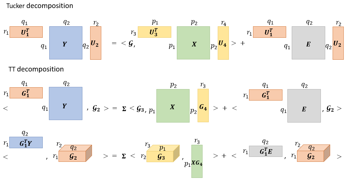
We next conduct dimension reduction to model (5) by TT decomposition. Suppose that $\mathscr{A}$ has TT ranks $(r_{\_}{1},r_{\_}{2},r_{\_}3)$, and it then has a TT decomposition $\mbox{\boldmath$\mathscr{A}$}=[[\boldsymbol{G}_{\_}1,\mbox{\boldmath$\mathscr{G}$}_{\_}2,\boldsymbol{\Sigma},\mbox{\boldmath$\mathscr{G}$}_{\_}{3},\boldsymbol{G}_{\_}{4}]]$, i.e.

$$[\mbox{\boldmath$\mathscr{A}$}]_{\_}2=(\boldsymbol{I}_{\_}{p_{\_}2}\otimes\boldsymbol{G}_{\_}1)[\mbox{\boldmath$\mathscr{G}$}_{\_}2]_{\_}2\boldsymbol{\Sigma}[\mbox{\boldmath$\mathscr{G}$}_{\_}{3}]_{\_}1(\boldsymbol{G}_{\_}{4}^{\top}\otimes\boldsymbol{I}_{\_}{p_{\_}{3}}),$$

where $\boldsymbol{G}_{\_}1^{\top}\boldsymbol{G}_{\_}1=\boldsymbol{I}_{\_}{r_{\_}1}$, $[\mbox{\boldmath$\mathscr{G}$}_{\_}2]_{\_}2^{\top}[\mbox{\boldmath$\mathscr{G}$}_{\_}2]_{\_}2=[\mbox{\boldmath$\mathscr{G}$}_{\_}3]_{\_}1[\mbox{\boldmath$\mathscr{G}$}_{\_}3]_{\_}1^{\top}=\boldsymbol{I}_{\_}{r_{\_}{2}}$, $\boldsymbol{G}_{\_}4^{\top}\boldsymbol{G}_{\_}4=\boldsymbol{I}_{\_}{r_{\_}3}$, and $\boldsymbol{\Sigma}\in\mathbb{R}^{r_{\_}2\times r_{\_}2}$ is a diagonal matrix. From model (5), $\operatorname*{vec}(\boldsymbol{Y}_{\_}i)=[\mbox{\boldmath$\mathscr{A}$}]_{\_}2\operatorname*{vec}(\boldsymbol{X}_{\_}i)+\operatorname*{vec}(\boldsymbol{E}_{\_}i)$, and it then holds that

$$[\mbox{\boldmath$\mathscr{G}$}_{\_}2]_{\_}{2}^{\top}\operatorname*{vec}(\boldsymbol{G}_{\_}1^{\top}\boldsymbol{Y}_{\_}i)=\boldsymbol{\Sigma}[\mbox{\boldmath$\mathscr{G}$}_{\_}{3}]_{\_}1\operatorname*{vec}(\boldsymbol{X}_{\_}i\boldsymbol{G}_{\_}4)+[\mbox{\boldmath$\mathscr{G}$}_{\_}2]_{\_}{2}^{\top}\operatorname*{vec}(\boldsymbol{G}_{\_}1^{\top}\boldsymbol{E}_{\_}i),$$ (7)

where $[\mbox{\boldmath$\mathscr{G}$}_{\_}2]_{\_}{2}^{\top}\operatorname*{vec}(\boldsymbol{G}_{\_}1^{\top}\boldsymbol{Y}_{\_}i)=\langle\boldsymbol{G}_{\_}1^{\top}\boldsymbol{Y}_{\_}i,\mbox{\boldmath$\mathscr{G}$}_{\_}2\rangle$, and $[\mbox{\boldmath$\mathscr{G}$}_{\_}{3}]_{\_}1\operatorname*{vec}(\boldsymbol{X}_{\_}i\boldsymbol{G}_{\_}4)=\langle\mbox{\boldmath$\mathscr{G}$}_{\_}{3},\boldsymbol{X}_{\_}i\boldsymbol{G}_{\_}4\rangle$; see Figure 1 for its illustration. It can be seen that the responses $\boldsymbol{Y}_{\_}i\in\mathbb{R}^{q_{\_}1\times q_{\_}2}$ and predictors $\boldsymbol{X}_{\_}i\in\mathbb{R}^{p_{\_}1\times p_{\_}2}$ are first summarized into response factors $[\mbox{\boldmath$\mathscr{G}$}_{\_}2]_{\_}{2}^{\top}\operatorname*{vec}(\boldsymbol{G}_{\_}1^{\top}\boldsymbol{Y}_{\_}i)\in\mathbb{R}^{r_{\_}2}$ and predictor factors $[\mbox{\boldmath$\mathscr{G}$}_{\_}{3}]_{\_}1\operatorname*{vec}(\boldsymbol{X}_{\_}i\boldsymbol{G}_{\_}4)\in\mathbb{R}^{r_{\_}2}$, respectively, and we then regress the response factors on predictor ones in the element-wise sense since the coefficient matrix $\boldsymbol{\Sigma}\in\mathbb{R}^{r_{\_}2\times r_{\_}2}$ is diagonal.

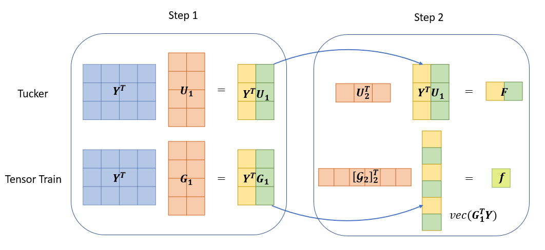
On one hand, both models via Tucker and TT decomposition share similar two-stage procedures: summarizing responses and predictors into factors, and then regressing response factors on predictor ones. On the other hand, the two procedures are different in details. We next demonstrate how Tucker and TT decomposition conduct dimension reduction for responses $\boldsymbol{Y}$ in the first stage. Specifically, from (6) and (7), the $q_{\_}1$ variables along the first mode of $\boldsymbol{Y}\in\mathbb{R}^{q_{\_}1\times q_{\_}2}$ are first summarized into $r_{\_}1$ factors, $\boldsymbol{U}_{\_}1^{\top}\boldsymbol{Y}_{\_}i$ and $\boldsymbol{G}_{\_}1^{\top}\boldsymbol{Y}_{\_}i$, by Tucker and TT decomposition in the same way. When further compressing the second mode of $\boldsymbol{Y}\in\mathbb{R}^{q_{\_}1\times q_{\_}2}$, Tucker decomposition conducts dimension reduction for the $q_{\_}2$ variables within each of summarized $r_{\_}1$ factors, while TT decomposition does it for all summarized $q_{\_}2r_{\_}1$ factors; see Figure 2 for the illustration. Note that TT decomposition extracts response and predictor factors in a reverse order. Moreover, CP decomposition does not enjoy the above factor modeling interpretation.

Refer to caption
Figure 2: Illustration on how Tucker and TT decomposition extract response factors for a simple tensor regression with matrix-valued responses.

TT decomposition is more suitable for the data with nested, or hierarchical, structures, and an empirical example is given below (Montgomery,, 2006, Chpater 14). Consider a company that purchases raw material from $q_{\_}2=3$ different suppliers, and the purity of material is of interest. There are $q_{\_}1=4$ batches of raw material, with first two batches having relatively higher purity, available from each supplier, and $N$ determinations of purity are to be taken from each batch. Note that batches are nested under each supplier. As in Figure 2, TT decomposition first summarize the $q_{\_}1=4$ batches of raw material into $r_{\_}1=2$ factors for each supplier, and the two factors represent the higher and lower purity, respectively. Each supplier has two factors, and there are six ones in total. TT decomposition further summarizes these six factors into one. Note that the suppliers may be of different quality, and it hence is not suitable for Tucker decomposition to summarize the $q_{\_}2=3$ suppliers within each of $r_{\_}1=2$ factors, respectively.

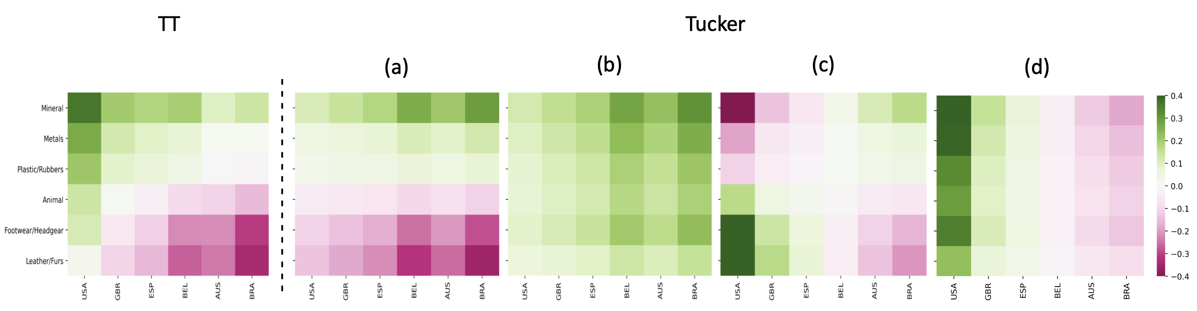
TT decomposition also enjoys advantages for the data with a seemingly factorial structure by creating much less number of factors. For example, consider the monthly international import trade data from January 2010 to December 2019, and we choose $q_{\_}1=6$ product categories and $q_{\_}2=6$ countries such that these countries have different preferred product categories for importation. The predictors are set to $\boldsymbol{X}_{\_}i=\boldsymbol{Y}_{\_}{i-1}^{\top}$. TT and Tucker decomposition are applied to coefficient tensor $\mathscr{A}$ with ranks $(2,1,1)$ and $(2,2,1,1)$, respectively, such that they have similar estimation errors and the same number of parameters. Note that Tucker decomposition leads to four response factors, while there is only one for TT decomposition. Heatmaps of their loading matrices are presented in Figure 3 and, from the one for TT decomposition, the products and countries are coherent to each other although it is factorial. As a result, we need at least four factors from Tucker decomposition to represent it.

Finally, the models via Tucker and TT decomposition will involve different numbers of parameters in the second stage, and they correspond to the sizes of $\mathscr{G}$ at (6) and $\boldsymbol{\Sigma}$ at (7), which are $\prod_{\_}{i=1}^{4}r_{\_}i$ and $r_{\_}2$, respectively. Consider a model with both responses and predictors being third-order tensors, and suppose that the coefficient tensor $\mathscr{A}$ has Tucker ranks $(r_{\_}1,\cdots,r_{\_}6)$ with $r_{\_}i$’s being as small as five. As a result, the size of $\mathscr{G}$ is $5^{6}=15625$. In fact, Tucker decomposition has a poor performance for a higher order tensor (Oseledets,, 2011), and the situation is much more serious for regression problems. In the meanwhile, we can always control the size of $\boldsymbol{\Sigma}$ within a reasonable range. This further confirms the necessity of TT decomposition for tensor regression, especially for responses and predictors with high order tensors.

3 Tensor train regression for high-dimensional data

3.1 Tensor train regression

This subsection considers a general regression with tensor-valued responses and predictors,

$$\mbox{\boldmath$\mathscr{Y}$}_{\_}i=\langle\mbox{\boldmath$\mathscr{A}$},\mbox{\boldmath$\mathscr{X}$}_{\_}i\rangle+\mbox{\boldmath$\mathscr{E}$}_{\_}i\hskip 5.69054pt\text{for}\hskip 5.69054pt1\leq i\leq N,$$ (8)

where $\mbox{\boldmath$\mathscr{Y}$}_{\_}i\in\mathbb{R}^{q_{\_}1\times q_{\_}2\times\cdots\times q_{\_}n}$, $\mbox{\boldmath$\mathscr{X}$}_{\_}i\in\mathbb{R}^{p_{\_}1\times p_{\_}2\times\cdots\times p_{\_}m}$, $\mbox{\boldmath$\mathscr{A}$}\in\mathbb{R}^{q_{\_}1\times\cdots\times q_{\_}n\times p_{\_}1\times\cdots\times p_{\_}m}$ is the coefficient tensor, $\mbox{\boldmath$\mathscr{E}$}_{\_}i\in\mathbb{R}^{q_{\_}1\times q_{\_}2\times\cdots\times q_{\_}n}$ is the error term, and $N$ is the sample size. As in Section 2.2, the responses $\mbox{\boldmath$\mathscr{Y}$}_{\_}i$ are supposed to have a nested or hierarchical structure, and its $j$th mode is nested under each level of $(j+1)$th mode for all $1\leq j\leq n-1$. In the meanwhile, it is common that some modes are arranged in a factorial layout and other modes are nested, and this corresponds to a nested-factorial design in the area of experimental designs (Montgomery,, 2006, Chpater 14). In fact, all modes may even be factorial. For these cases, the modes are first arranged according to our experiences and, for these modes with no preference, we may simply put the ones with more levels, i.e. larger values of $q_{\_}j$’s, at lower places since they will be summarized into lower dimensional factors earlier. Finally, since the predictor factors are extracted in a reverse order, we assume that the predictors $\mbox{\boldmath$\mathscr{X}$}_{\_}i$ also have a nested structure, while its $j$th mode is nested under each level of $(j-1)$th mode for all $2\leq j\leq m$.

Suppose that the coefficient tensor $\mathscr{A}$ has tensor train (TT) ranks $R=(r_{\_}{1},r_{\_}{2},\ldots,r_{\_}{m+n-1})$, i.e. $r_{\_}i=\operatorname*{rank}([\mbox{\boldmath$\mathscr{A}$}]_{\_}i)$ for all $1\leq i\leq m+n-1$, and then the parameter space can be denoted by

$$\boldsymbol{\Theta}_{\_}1(R)=\{\mbox{\boldmath$\mathscr{A}$}\in\mathbb{R}^{q_{\_}1\times\cdots\times q_{\_}n\times p_{\_}1\times\cdots\times p_{\_}m}:\operatorname*{rank}([\mbox{\boldmath$\mathscr{A}$}]_{\_}i)\leq r_{\_}i\text{ for all }1\leq i\leq m+n-1\}.$$

From Proposition 1, we have $\mbox{\boldmath$\mathscr{A}$}=[[\boldsymbol{G}_{\_}1,\mbox{\boldmath$\mathscr{G}$}_{\_}2,\ldots,\boldsymbol{\Sigma},\ldots,\mbox{\boldmath$\mathscr{G}$}_{\_}{n+m-1},\boldsymbol{G}_{\_}{n+m}]]$, i.e.

$$[\mbox{\boldmath$\mathscr{A}$}]_{\_}n=(\boldsymbol{I}_{\_}{q_{\_}2\cdots q_{\_}n}\otimes\boldsymbol{G}_{\_}1)\cdots(\boldsymbol{I}_{\_}{q_{\_}n}\otimes[\mbox{\boldmath$\mathscr{G}$}_{\_}{n-1}]_{\_}2)[\mbox{\boldmath$\mathscr{G}$}_{\_}n]_{\_}2\boldsymbol{\Sigma}[\mbox{\boldmath$\mathscr{G}$}_{\_}{n+1}]_{\_}1([\mbox{\boldmath$\mathscr{G}$}_{\_}{n+2}]_{\_}1\otimes\boldsymbol{I}_{\_}{p_{\_}{1}})\cdots(\boldsymbol{G}_{\_}{n+m}^{\top}\otimes\boldsymbol{I}_{\_}{p_{\_}{1}\cdots p_{\_}{m-1}}),$$

where $\boldsymbol{G}_{\_}1^{\top}\boldsymbol{G}_{\_}1=\boldsymbol{I}_{\_}{r_{\_}1}$, $[\mbox{\boldmath$\mathscr{G}$}_{\_}i]_{\_}2^{\top}[\mbox{\boldmath$\mathscr{G}$}_{\_}i]_{\_}2=\boldsymbol{I}_{\_}{r_{\_}i}$ for $2\leq i\leq n$, $[\mbox{\boldmath$\mathscr{G}$}_{\_}i]_{\_}1[\mbox{\boldmath$\mathscr{G}$}_{\_}i]_{\_}1^{\top}=\boldsymbol{I}_{\_}{r_{\_}{i-1}}$ for $n+1\leq i\leq n+m-1$, $\boldsymbol{G}_{\_}{n+m}^{\top}\boldsymbol{G}_{\_}{n+m}=\boldsymbol{I}_{\_}{r_{\_}{n+m-1}}$, and $\boldsymbol{\Sigma}\in\mathbb{R}^{r_{\_}n\times r_{\_}n}$ is diagonal. Note that $\operatorname*{vec}(\mbox{\boldmath$\mathscr{Y}$}_{\_}i)=[\mbox{\boldmath$\mathscr{A}$}]_{\_}n\operatorname*{vec}(\mbox{\boldmath$\mathscr{X}$}_{\_}i)+\operatorname*{vec}(\mbox{\boldmath$\mathscr{E}$}_{\_}i)$, and then model (8) can be rewritten into

$\displaystyle\begin{split}[\mbox{\boldmath$\mathscr{G}$}_{\_}n]_{\_}{2}^{\top}(\boldsymbol{I}_{\_}{q_{\_}n}\otimes[\mbox{\boldmath$\mathscr{G}$}_{\_}{n-1}]_{\_}{2}^{\top})&\cdots(\boldsymbol{I}_{\_}{q_{\_}2\cdots q_{\_}n}\otimes\boldsymbol{G}_{\_}{1}^{\top})\operatorname*{vec}(\mbox{\boldmath$\mathscr{Y}$}_{\_}i)\\ &=\boldsymbol{\Sigma}\{[\mbox{\boldmath$\mathscr{G}$}_{\_}{n+1}]_{\_}1([\mbox{\boldmath$\mathscr{G}$}_{\_}{n+2}]_{\_}1\otimes\boldsymbol{I}_{\_}{p_{\_}{1}})\cdots(\boldsymbol{G}_{\_}{n+m}^{\top}\otimes\boldsymbol{I}_{\_}{p_{\_}{1}\cdots p_{\_}{m-1}})\operatorname*{vec}(\mbox{\boldmath$\mathscr{X}$}_{\_}i)\}\\ &\hskip 71.13188pt+[\mbox{\boldmath$\mathscr{G}$}_{\_}n]_{\_}{2}^{\top}(\boldsymbol{I}_{\_}{q_{\_}n}\otimes[\mbox{\boldmath$\mathscr{G}$}_{\_}{n-1}]_{\_}{2}^{\top})\cdots(\boldsymbol{I}_{\_}{q_{\_}2\cdots q_{\_}n}\otimes\boldsymbol{G}_{\_}{1}^{\top})\operatorname*{vec}(\mbox{\boldmath$\mathscr{E}$}_{\_}i).\end{split}$ (9)

For simplicity, we call the above model tensor train regression.

Similar to the illustrative example in Section 2.2, model (9) consists of two stages: summarizing factors and conducting regression on the resulting factors in the element-wise sense. In the first stage, we first perform dimension reduction for $\mbox{\boldmath$\mathscr{Y}$}_{\_}i$ along the first mode by summarizing $q_{\_}1$ variables into $r_{\_}1$ factors through $\boldsymbol{G}_{\_}1$, then compress the stacked first and second modes by summarizing $r_{\_}1q_{\_}2$ factors into $r_{\_}2$ ones through $\mbox{\boldmath$\mathscr{G}$}_{\_}2$, and so on. The procedure will end until we extract $r_{\_}k$ factors from responses. On the contrary, the factor-extracting procedure for $\mbox{\boldmath$\mathscr{X}$}_{\_}i$ follows a reverse order, and it rolls up from the last mode until the first mode one-by-one. At the end, it will also produce $r_{\_}k$ factors from predictors; see the supplementary file for the illustration on how to extract factors from a third order predictor tensor. Finally, the second stage regresses $r_{\_}k$ response factors on $r_{\_}k$ predictor ones with the coefficient matrix $\boldsymbol{\Sigma}$ being diagonal, and hence there are only $r_{\_}k$ parameters involved.

Consider the ordinary least squares (OLS) estimation for linear regression at (9),

$$\mbox{\boldmath$\mathscr{\widehat{A}}$}_{\_}{\mathrm{LR}}=\arg\min_{\_}{\mbox{\boldmath$\mathscr{A}$}\in\boldsymbol{\Theta}_{\_}1(R)}\sum_{\_}{i=1}^{N}\|\mbox{\boldmath$\mathscr{Y}$}_{\_}i-\langle\mbox{\boldmath$\mathscr{A}$},\mbox{\boldmath$\mathscr{X}$}_{\_}i\rangle\|_{\_}{\mathrm{F}}^{2}.$$

Let $P=\prod_{\_}{i=1}^{m}p_{\_}i$, $Q=\prod_{\_}{i=1}^{n}q_{\_}i$, $r_{\_}{\mathrm{max}}=\mathrm{max}\{r_{\_}1,r_{\_}2,\ldots,r_{\_}{m+n-1}\}$ and $d_{\_}{\mathrm{LR}}=4r_{\_}{\mathrm{max}}^{2}(\sum_{\_}{i=1}^{m}p_{\_}i+\sum_{\_}{i=1}^{n}q_{\_}i)+2r_{\_}{\mathrm{max}}$. In order to establish nonasymptotic properties for the OLS estimator, we first make two assumptions on predictors $\boldsymbol{x}_{\_}i=\operatorname*{vec}(\mbox{\boldmath$\mathscr{X}$}_{\_}i)\in\mathbb{R}^{P}$ and error terms $\boldsymbol{e}_{\_}i=\operatorname*{vec}(\mbox{\boldmath$\mathscr{E}$}_{\_}{i})\in\mathbb{R}^{Q}$, respectively, and they both are commonly used in the literature (Wainwright,, 2019).

Assumption 1.

Predictors $\{\boldsymbol{x}_{\_}i\}$ are $i.i.d$ with $\mathbb{E}(\boldsymbol{x}_{\_}i)=0$, $\mathrm{var}(\boldsymbol{x}_{\_}i)=\boldsymbol{\Sigma}_{\_}x$ and $\sigma^{2}$-sub-Gaussian distribution. There exist constants $0<c_{\_}{x}<C_{\_}{x}<\infty$ such that $c_{\_}x\boldsymbol{I}_{\_}P\leq\boldsymbol{\Sigma}_{\_}x\leq C_{\_}x\boldsymbol{I}_{\_}P$.

Assumption 2.

Error terms $\{\boldsymbol{e}_{\_}i\}$ are $i.i.d$ and, conditional on $\boldsymbol{x}_{\_}i$, $\boldsymbol{e}_{\_}i$ has mean zero and follows $\kappa^{2}$-sub-Gaussian distribution.

Theorem 1.

Suppose that Assumptions 1 and 2 hold, and the true coefficient tensor $\mbox{\boldmath$\mathscr{A}$}^{*}$ has TT ranks $R=(r_{\_}1,r_{\_}2,\ldots,r_{\_}{m+n-1})$. If the sample size $N\gtrsim\max\{\sigma^{2}/c_{\_}x,\sigma^{4}/c_{\_}x^{2}\}\cdot\{[0.5(m+n)+2]\log[6\sqrt{C_{\_}x/c_{\_}x}(m+n+1)]d_{\_}{\mathrm{LR}}+\log Q\}$, then

$\displaystyle\|\mbox{\boldmath$\mathscr{\widehat{A}}$}_{\_}{\mathrm{LR}}-\mbox{\boldmath$\mathscr{A}$}^{*}\|_{\_}{\mathrm{F}}$ $\displaystyle\leq\frac{\delta c_{\_}1\kappa}{c_{\_}x^{2}}\sqrt{\frac{C_{\_}{x}[0.5(m+n)+2]\log(6m+6n+6)d_{\_}{\mathrm{LR}}}{N}}$

for some $\delta>1$ with probability at least

$\displaystyle 1$ $\displaystyle-2Q\exp\{-cN\min\left(c_{\_}x/\sigma^{2},c_{\_}x^{2}/\sigma^{4}\right)+[0.5(m+n)+2]\log[6\sqrt{C_{\_}x/c_{\_}x}(m+n+1)]d_{\_}{\mathrm{LR}}\}$
$\displaystyle-\exp\{-\delta^{2}[0.5(m+n)+2]\log(6m+6n+6)d_{\_}{\mathrm{LR}}\},$

where $c$ and $c_{\_}1$ are positive constants given in the proof.

From the above theorem, when $m$ and $n$ are fixed, and the parameters $c_{\_}x$, $C_{\_}x$, $\sigma^{2}$ and $\kappa^{2}$ are bounded away from zero and infinity, we then have $\|\mbox{\boldmath$\mathscr{\widehat{A}}$}_{\_}{\mathrm{LR}}-\mbox{\boldmath$\mathscr{A}$}^{*}\|_{\_}{\mathrm{F}}=O_{\_}p(\sqrt{d_{\_}{\mathrm{LR}}/N})$, where $d_{\_}{\mathrm{LR}}$ is the corresponding model complexity. Moreover, if Tucker decomposition is applied to the coefficient tensor $\mathscr{A}$ with Tucker ranks $(r_{\_}1,\ldots,r_{\_}{m+n})$, then the resulting OLS estimator will have the convergence rate of $\sqrt{d_{\_}{\mathrm{Tucker}}/N}$, and the model complexity is $d_{\_}{\mathrm{Tucker}}=\prod_{\_}{i=1}^{m+n}r_{\_}i+\sum_{\_}{i=1}^{m}p_{\_}ir_{\_}i+\sum_{\_}{i=1}^{n}q_{\_}ir_{\_}i$; see Han et al., 2022a . The term of $\prod_{\_}{i=1}^{m+n}r_{\_}i$ will result in a huge number even for very low ranks and small values of $m$ and $n$, and this actually hinders the application of Tucker decomposition on tensor regression with higher order response and predictor tensors. Finally, the proof of Theorem 1 heavily depends on an delicate analysis on the covering numbers of $\mathscr{A}$ under TT decomposition, which is of interest independently.

3.2 Tensor train autoregression

We first consider a simple autoregressive (AR) model for tensor-valued time series $\{\mbox{\boldmath$\mathscr{Y}$}_{\_}t\}$,

$$\mbox{\boldmath$\mathscr{Y}$}_{\_}t=\langle\mbox{\boldmath$\mathscr{A}$},\mbox{\boldmath$\mathscr{Y}$}_{\_}{t-1}\rangle+\mbox{\boldmath$\mathscr{E}$}_{\_}t,$$ (10)

where $\mbox{\boldmath$\mathscr{Y}$}_{\_}t\in\mathbb{R}^{p_{\_}1\times p_{\_}2\times\cdots\times p_{\_}d}$, $\mbox{\boldmath$\mathscr{A}$}\in\mathbb{R}^{p_{\_}1\times\cdots\times p_{\_}d\times p_{\_}1\times\cdots\times p_{\_}d}$ is the coefficient tensor, and $\mbox{\boldmath$\mathscr{E}$}_{\_}t\in\mathbb{R}^{p_{\_}1\times p_{\_}2\times\cdots\times p_{\_}d}$ is the error term. As in Section 3.1, we rearrange $\mbox{\boldmath$\mathscr{Y}$}_{\_}t$ into a nested structure, and its $j$th mode is nested under each level of $(j+1)$th mode for all $1\leq j\leq d-1$. Moreover, denote by $\mbox{\boldmath$\mathscr{Y}$}_{\_}{t}^{\top}$ the rearrangement of $\mbox{\boldmath$\mathscr{Y}$}_{\_}{t}$ such that the $1,2,\ldots,d$-th modes of $\mbox{\boldmath$\mathscr{Y}$}_{\_}{t}$ correspond to the $d,\ldots,2,1$-th modes of $\mbox{\boldmath$\mathscr{Y}$}_{\_}{t}^{\top}$, respectively. As a result, $\mbox{\boldmath$\mathscr{Y}$}_{\_}{t-1}^{\top}$ also has a nested structure but with a reverse order, and hence model (10) can be reorganized into

$$\mbox{\boldmath$\mathscr{Y}$}_{\_}t=\langle\mathcal{M}(\mbox{\boldmath$\mathscr{A}$}),\mbox{\boldmath$\mathscr{Y}$}_{\_}{t-1}^{\top}\rangle+\mbox{\boldmath$\mathscr{E}$}_{\_}t,$$

where $\mathcal{M}(\mbox{\boldmath$\mathscr{A}$})$ is the rearrangement of $\mathscr{A}$ according to $\mbox{\boldmath$\mathscr{Y}$}_{\_}{t-1}^{\top}$. Suppose that the reshaped coefficient tensor $\mathcal{M}(\mbox{\boldmath$\mathscr{A}$})$ has low TT ranks $R=(r_{\_}1,r_{\_}2,\ldots,r_{\_}{2d-1})$, i.e. $r_{\_}i=\operatorname*{rank}([\mathcal{M}(\mbox{\boldmath$\mathscr{A}$})]_{\_}i)$ for all $1\leq i\leq 2d-1$, and the corresponding parameter space can then be denoted by

$$\boldsymbol{\Theta}_{\_}2(R)=\{\mbox{\boldmath$\mathscr{A}$}\in\mathbb{R}^{p_{\_}1\times\cdots\times p_{\_}d\times p_{\_}1\times\cdots\times p_{\_}d}:\operatorname*{rank}([\mathcal{M}(\mbox{\boldmath$\mathscr{A}$})]_{\_}i)\leq r_{\_}i\text{ for all }1\leq i\leq 2d-1\}.$$

For simplicity, we call model (10), together with the parameter space of $\boldsymbol{\Theta}_{\_}2(R)$, tensor train autoregression with order one, and its physical interpretation is similar to that of tensor regression.

For an observed time series $\{\mbox{\boldmath$\mathscr{Y}$}_{\_}0,\mbox{\boldmath$\mathscr{Y}$}_{\_}1,\ldots,\mbox{\boldmath$\mathscr{Y}$}_{\_}N\}$ generated by model (10) with TT ranks $R=(r_{\_}1,r_{\_}2,\ldots,r_{\_}{2d-1})$, the OLS estimation can be defined as

$$\mbox{\boldmath$\mathscr{\widehat{A}}$}_{\_}{\mathrm{AR}}=\arg\min_{\_}{\mbox{\boldmath$\mathscr{A}$}\in\boldsymbol{\Theta}_{\_}2(R)}\sum_{\_}{t=1}^{N}\|\mbox{\boldmath$\mathscr{Y}$}_{\_}{t}-\langle\mbox{\boldmath$\mathscr{A}$},\mbox{\boldmath$\mathscr{Y}$}_{\_}{t-1}\rangle\|_{\_}{\mathrm{F}}^{2}.$$ (11)
Assumption 3.

Sequential matricization $[\mbox{\boldmath$\mathscr{A}$}]_{\_}d$ has the spectral radius strictly less than one.

Assumption 4.

For the error term, let $\boldsymbol{e}_{\_}t=\operatorname*{vec}(\mbox{\boldmath$\mathscr{E}$}_{\_}{t})=\boldsymbol{\Sigma}_{\_}e^{1/2}\boldsymbol{\xi}_{\_}t$ and $P=\prod_{\_}{i=1}^{d}p_{\_}i$. Random vectors $\{\boldsymbol{\xi}_{\_}t\}$ are $i.i.d.$ with $\mathbb{E}(\boldsymbol{\xi}_{\_}t)=0$ and $\mathrm{var}(\boldsymbol{\xi}_{\_}t)=\boldsymbol{I}_{\_}P$, the entries $(\boldsymbol{\xi}_{\_}{tj})_{\_}{1\leq j\leq P}$ of $\boldsymbol{\xi}_{\_}t$ are mutually independent and $\kappa^{2}$-sub-Gaussian distributed, and there exist constants $0<c_{\_}{e}<C_{\_}{e}<\infty$ such that $c_{\_}{e}\boldsymbol{I}_{\_}P\leq\boldsymbol{\Sigma}_{\_}e\leq C_{\_}{e}\boldsymbol{I}_{\_}P$.

Assumption 3 is necessary and sufficient for the existence of a unique strictly stationary solution to model (10). The sub-Gaussian condition in Assumption 4 is weaker than the commonly used Gaussian assumption in the literature (Basu and Michailidis,, 2015), and it thanks to the established martingale-based concentration bound, which is a nontrival task for high-dimensional time series and is of interest independently, in the technical proofs.

We next establish the estimation error bound of $\mbox{\boldmath$\mathscr{\widehat{A}}$}_{\_}{\mathrm{AR}}$, which will rely on the temporal and cross-sectional dependence of $\{\mbox{\boldmath$\mathscr{Y}$}_{\_}t\}$ (Basu and Michailidis,, 2015). To this end, we first define a matrix polynomial $\mbox{\boldmath$\mathscr{A}$}(z):=\boldsymbol{I}_{\_}P-[\mbox{\boldmath$\mathscr{A}$}]_{\_}dz$, where $z\in\mathbb{C}$ with $\mathbb{C}$ being the complex space, and its conjugate transpose is denoted by $\bar{\mbox{\boldmath$\mathscr{A}$}}(z)$. Let

$$\mu_{\_}{\mathrm{min}}(\mbox{\boldmath$\mathscr{A}$})=\mathrm{min}_{\_}{|z|=1}\lambda_{\_}{\mathrm{min}}(\bar{\mbox{\boldmath$\mathscr{A}$}}(z)\mbox{\boldmath$\mathscr{A}$}(z))\hskip 14.22636pt\text{and}\hskip 14.22636pt\mu_{\_}{\mathrm{max}}(\mbox{\boldmath$\mathscr{A}$})=\mathrm{max}_{\_}{|z|=1}\lambda_{\_}{\mathrm{max}}(\bar{\mbox{\boldmath$\mathscr{A}$}}(z)\mbox{\boldmath$\mathscr{A}$}(z)).$$

We then denote $r_{\_}{\mathrm{max}}=\mathrm{max}(r_{\_}1,r_{\_}2,\cdots,r_{\_}{2d-1})$, $d_{\_}{\mathrm{AR}}=8r_{\_}{\mathrm{max}}^{2}\sum_{\_}{i=1}^{d}p_{\_}i+2r_{\_}{\mathrm{max}}$, $\kappa_{\_}U=C_{\_}{e}/\mu_{\_}{\mathrm{min}}(\mbox{\boldmath$\mathscr{A}$}^{*})$ and $\kappa_{\_}L=c_{\_}{e}/\mu_{\_}{\mathrm{max}}(\mbox{\boldmath$\mathscr{A}$}^{*})$, where $\mbox{\boldmath$\mathscr{A}$}^{*}(z)$ is the polynomial with $\mbox{\boldmath$\mathscr{A}$}=\mbox{\boldmath$\mathscr{A}$}^{*}$, and $\mbox{\boldmath$\mathscr{A}$}^{*}$ is the true coefficient tensor.

Theorem 2.

Suppose that Assumptions 3 and 4 hold, and the reshaped true coefficient tensor $\mathcal{M}(\mbox{\boldmath$\mathscr{A}$}^{*})$ has TT ranks $R=(r_{\_}1,r_{\_}2,\ldots,r_{\_}{2d-1})$. If $N\gtrsim\max\left(\kappa^{2}\kappa_{\_}U/\kappa_{\_}L,\kappa^{4}\kappa_{\_}U^{2}/\kappa_{\_}L^{2}\right)\cdot(d+2)\log[6\sqrt{\kappa_{\_}U/\kappa_{\_}L}(2d+1)]d_{\_}{\mathrm{AR}}$, then

$\displaystyle\|{\mbox{\boldmath$\mathscr{\widehat{A}}$}_{\_}{\mathrm{AR}}-\mbox{\boldmath$\mathscr{A}$}^{*}}\|_{\_}{\mathrm{F}}$ $\displaystyle\leq\frac{\delta c_{\_}1\kappa}{\kappa_{\_}L}\sqrt{\frac{C_{\_}{e}\kappa_{\_}U(d+2)\log(12d+6)d_{\_}{\mathrm{AR}}}{N}}$

for some $\delta>1$ with probability at least

$\displaystyle 1-$ $\displaystyle 2\exp\left\{-cN\min\left(\frac{\kappa_{\_}L}{\kappa^{2}\kappa_{\_}U},\frac{\kappa_{\_}L^{2}}{\kappa^{4}\kappa_{\_}U^{2}}\right)+(d+2)\log\left[6\sqrt{\frac{\kappa_{\_}U}{\kappa_{\_}L}}(2d+1)\right]d_{\_}{\mathrm{AR}}\right\}$
$\displaystyle-$ $\displaystyle\exp\left\{-\delta^{2}(d+2)\log(12d+6)d_{\_}{\mathrm{AR}}\right\},$

where $c$ and $c_{\_}1$ are positive constants given in the proof.

From the above theorem, when $d$ is fixed, and the parameters $c_{\_}e$, $C_{\_}e$, $\kappa^{2}$, $\mu_{\_}{\mathrm{min}}(\mbox{\boldmath$\mathscr{A}$}^{*})$ and $\mu_{\_}{\mathrm{max}}(\mbox{\boldmath$\mathscr{A}$}^{*})$ are bounded away from zero and infinity, we then have $\|\mbox{\boldmath$\mathscr{\widehat{A}}$}_{\_}{\mathrm{AR}}-\mbox{\boldmath$\mathscr{A}$}^{*}\|_{\_}{\mathrm{F}}=O_{\_}{P}(\sqrt{d_{\_}{\mathrm{AR}}/N})$, where $d_{\_}{\mathrm{AR}}$ the corresponding model complexity.

The AR model with lag one at model (10) may not be enough to fit the data with more complicated autocorrelation structures, and we next extend it to the case with a general order $p$,

$$\mbox{\boldmath$\mathscr{Y}$}_{\_}t=\langle\mbox{\boldmath$\mathscr{A}$}_{\_}1,\mbox{\boldmath$\mathscr{Y}$}_{\_}{t-1}\rangle+\langle\mbox{\boldmath$\mathscr{A}$}_{\_}2,\mbox{\boldmath$\mathscr{Y}$}_{\_}{t-2}\rangle+\ldots+\langle\mbox{\boldmath$\mathscr{A}$}_{\_}p,\mbox{\boldmath$\mathscr{Y}$}_{\_}{t-p}\rangle+\mbox{\boldmath$\mathscr{E}$}_{\_}t.$$ (12)

We first stack $\mbox{\boldmath$\mathscr{Y}$}_{\_}{t-1},\ldots,\mbox{\boldmath$\mathscr{Y}$}_{\_}{t-p}$ into a new tensor $\mbox{\boldmath$\mathscr{Y}$}_{\_}{t-1:t-p}\in\mathbb{R}^{p\times p_{\_}1\times\cdots\times p_{\_}d}$ with $(d+1)$ modes, and then $\mbox{\boldmath$\mathscr{A}$}_{\_}{1},\ldots,\mbox{\boldmath$\mathscr{A}$}_{\_}{p}$ are also stacked into another new tensor $\mbox{\boldmath$\mathscr{A}$}_{\_}{1:p}\in\mathbb{R}^{p_{\_}1\times\cdots\times p_{\_}d\times p\times p_{\_}1\times\cdots\times p_{\_}d}$ with $(2d+1)$ modes accordingly. Note that, for $\mbox{\boldmath$\mathscr{Y}$}_{\_}t$, its $j$th mode is nested under each level of $(j+1)$th mode for all $1\leq j\leq d-1$, and we here actually put the new mode of lags at the lowest place in the hierarchical structure. It certainly can be at the highest place, i.e. all modes are nested under each lag, and the notations can be adjusted accordingly. On the other hand, as in Wang et al., 2021b , such arrangement will make it convenient to further explore the possible low-rank structure along lags.

Denote by $\mbox{\boldmath$\mathscr{Y}$}_{\_}{t-1:t-p}^{\top}$ the rearrangement of $\mbox{\boldmath$\mathscr{Y}$}_{\_}{t-1:t-p}$ such that the $1,2,\ldots,(d+1)$-th modes of $\mbox{\boldmath$\mathscr{Y}$}_{\_}{t-1:t-p}$ correspond to the $(d+1),\ldots,2,1$-th modes of $\mbox{\boldmath$\mathscr{Y}$}_{\_}{t-1:t-p}^{\top}$, respectively. As a result, model (12) can be rewritten into

$$\mbox{\boldmath$\mathscr{Y}$}_{\_}t=\langle\mbox{\boldmath$\mathscr{A}$}_{\_}{1:p},\mbox{\boldmath$\mathscr{Y}$}_{\_}{t-1:t-p}\rangle+\mbox{\boldmath$\mathscr{E}$}_{\_}t\hskip 14.22636pt\text{or}\hskip 14.22636pt\mbox{\boldmath$\mathscr{Y}$}_{\_}t=\langle\mathcal{M}(\mbox{\boldmath$\mathscr{A}$}_{\_}{1:p}),\mbox{\boldmath$\mathscr{Y}$}_{\_}{t-1:t-p}^{\top}\rangle+\mbox{\boldmath$\mathscr{E}$}_{\_}t,$$ (13)

where $\mathcal{M}(\mbox{\boldmath$\mathscr{A}$}_{\_}{1:p})$ is the rearrangement of $\mbox{\boldmath$\mathscr{A}$}_{\_}{1:p}$ according to $\mbox{\boldmath$\mathscr{Y}$}_{\_}{t-1:t-p}^{\top}$. Suppose that the reshaped coefficient tensor $\mathcal{M}(\mbox{\boldmath$\mathscr{A}$}_{\_}{1:p})$ has low TT ranks $R=(r_{\_}1,r_{\_}2,\ldots,r_{\_}{2d})$, i.e. $r_{\_}i=\operatorname*{rank}([\mathcal{M}(\mbox{\boldmath$\mathscr{A}$})]_{\_}i)$ for all $1\leq i\leq 2d$, and then the parameter space for model (13) can be denoted by

$$\boldsymbol{\Theta}_{\_}3(R)=\{\mbox{\boldmath$\mathscr{A}$}\in\mathbb{R}^{p_{\_}1\times\cdots\times p_{\_}d\times p\times p_{\_}1\times\cdots\times p_{\_}d}:\operatorname*{rank}([\mathcal{M}(\mbox{\boldmath$\mathscr{A}$})]_{\_}i)\leq r_{\_}i\text{ for all }1\leq i\leq 2d\}.$$

We refer the tensor train autoregression with the order of $p$ to model (12) or (13) with the parameter space of $\boldsymbol{\Theta}_{\_}3(R)$. For a generated time series $\{\mbox{\boldmath$\mathscr{Y}$}_{\_}{1-p},\ldots,\mbox{\boldmath$\mathscr{Y}$}_{\_}0,\mbox{\boldmath$\mathscr{Y}$}_{\_}1,\ldots,\mbox{\boldmath$\mathscr{Y}$}_{\_}N\}$, the OLS estimation is defined as

$$\mbox{\boldmath$\mathscr{\widehat{A}}$}_{\_}{1:p}=\arg\min_{\_}{\mbox{\boldmath$\mathscr{A}$}\in\boldsymbol{\Theta}_{\_}3(R)}\sum_{\_}{t=1}^{N}\|\mbox{\boldmath$\mathscr{Y}$}_{\_}{t}-\langle\mbox{\boldmath$\mathscr{A}$}_{\_}{1:p},\mbox{\boldmath$\mathscr{Y}$}_{\_}{t-1:t-p}\rangle\|_{\_}{\mathrm{F}}^{2}.$$ (14)

The matrix polynomial for model (12) can be defined as $\mbox{\boldmath$\mathscr{A}$}(z):=\boldsymbol{I}_{\_}P-[\mbox{\boldmath$\mathscr{A}$}_{\_}1]_{\_}dz-\cdots-[\mbox{\boldmath$\mathscr{A}$}_{\_}p]_{\_}dz^{p}$, where $z\in\mathbb{C}$, and similarly the notations of $\mu_{\_}{\mathrm{min}}(\mbox{\boldmath$\mathscr{A}$})$ and $\mu_{\_}{\mathrm{max}}(\mbox{\boldmath$\mathscr{A}$})$. Let $r_{\_}{\mathrm{max}}=\mathrm{max}(r_{\_}1,r_{\_}2,\ldots,r_{\_}{2d})$, $d_{\_}{\mathrm{M}}=4r_{\_}{\mathrm{max}}^{2}(2\sum_{\_}{i=1}^{d}p_{\_}i+p)+2r_{\_}{\mathrm{max}}$, $\kappa_{\_}U=C_{\_}{e}/\mu_{\_}{\mathrm{min}}(\mbox{\boldmath$\mathscr{A}$}^{*})$ and $\kappa_{\_}L=c_{\_}{e}/\mu_{\_}{\mathrm{max}}(\mbox{\boldmath$\mathscr{A}$}^{*})$, where $\mbox{\boldmath$\mathscr{A}$}^{*}(z)$ is the polynomial with $\mbox{\boldmath$\mathscr{A}$}_{\_}{1:p}=\mbox{\boldmath$\mathscr{A}$}_{\_}{1:p}^{*}$, and $\mbox{\boldmath$\mathscr{A}$}_{\_}{1:p}^{*}$ is the true coefficient tensor.

Assumption 5.

The determinant of $\mbox{\boldmath$\mathscr{A}$}(z)$ is not equal to zero for all $|z|<1$.

Theorem 3.

Suppose that Assumptions 4-5 hold, and the reshaped true coefficient tensor $\mathcal{M}(\mbox{\boldmath$\mathscr{A}$}_{\_}{1:p}^{*})$ has TT ranks $R=(r_{\_}1,r_{\_}2,\ldots,r_{\_}{2d})$. If $N\gtrsim\max\left(\kappa^{2}\kappa_{\_}U/\kappa_{\_}L,\kappa^{4}\kappa_{\_}U^{2}/\kappa_{\_}L^{2}\right)\cdot(d+2)\log[12\sqrt{\kappa_{\_}U/\kappa_{\_}L}(d+1)]d_{\_}{\mathrm{M}}$, then

$\displaystyle\|\mbox{\boldmath$\mathscr{\widehat{A}}$}_{\_}{1:p}-\mbox{\boldmath$\mathscr{A}$}_{\_}{1:p}^{*}\|_{\_}{\mathrm{F}}$ $\displaystyle\leq\frac{\delta c_{\_}1\kappa}{\kappa_{\_}L}\sqrt{\frac{C_{\_}{e}\kappa_{\_}U(d+2)\log(12d+12)d_{\_}{M}}{N}}$

for some $\delta>1$ with probability at least

$\displaystyle 1-$ $\displaystyle 2\exp\left\{-cN\min\left(\frac{\kappa_{\_}L}{\kappa^{2}\kappa_{\_}U},\frac{\kappa_{\_}L^{2}}{\kappa^{4}\kappa_{\_}U^{2}}\right)+(d+2)\log\left[12\sqrt{\frac{\kappa_{\_}U}{\kappa_{\_}L}}(d+1)\right]d_{\_}{\mathrm{M}}\right\}$
$\displaystyle-$ $\displaystyle\exp\left\{-\delta^{2}(d+2)\log(12d+12)d_{\_}{\mathrm{M}}\right\}$

where $c$ and $c_{\_}1$ are positive constants given in the proof.

Note that $\|\mbox{\boldmath$\mathscr{\widehat{A}}$}_{\_}{1:p}-\mbox{\boldmath$\mathscr{A}$}_{\_}{1:p}^{*}\|_{\_}{\mathrm{F}}^{2}=\sum_{\_}{j=1}^{p}\|\mbox{\boldmath$\mathscr{\widehat{A}}$}_{\_}j-\mbox{\boldmath$\mathscr{A}$}_{\_}j^{*}\|_{\_}{\mathrm{F}}^{2}$, where $\mbox{\boldmath$\mathscr{\widehat{A}}$}_{\_}j$’s and $\mbox{\boldmath$\mathscr{A}$}_{\_}j^{*}$’s are OLS estimators and true coefficients, respectively. From Theorem 3, when $d$ is fixed, and the parameters $c_{\_}e$, $C_{\_}e$, $\kappa^{2}$, $\mu_{\_}{\mathrm{min}}(\mbox{\boldmath$\mathscr{A}$}^{*})$ and $\mu_{\_}{\mathrm{max}}(\mbox{\boldmath$\mathscr{A}$}^{*})$ are bounded away from zero and infinity, it holds that $\sum_{\_}{j=1}^{p}\|\mbox{\boldmath$\mathscr{\widehat{A}}$}_{\_}j-\mbox{\boldmath$\mathscr{A}$}_{\_}j^{*}\|_{\_}{\mathrm{F}}=O_{\_}{P}(\sqrt{d_{\_}{\mathrm{M}}/N})$, where $d_{\_}{\mathrm{M}}$ is the corresponding model complexity.

4 Algorithm and its theoretical justifications

4.1 Algorithm and convergence analysis

The three estimation problems in the previous section can be summarized into

$$\mbox{\boldmath$\mathscr{\widehat{A}}$}=\arg\min_{\_}{\mbox{\boldmath$\mathscr{A}$}\in\boldsymbol{\Theta}}\mathcal{L}_{\_}N(\mbox{\boldmath$\mathscr{A}$})\hskip 8.53581pt\text{with}\hskip 8.53581pt\mathcal{L}_{\_}N(\mbox{\boldmath$\mathscr{A}$})=\frac{1}{N}\sum_{\_}{i=1}^{N}\|\mbox{\boldmath$\mathscr{Y}$}_{\_}i-\langle\mbox{\boldmath$\mathscr{A}$},\mbox{\boldmath$\mathscr{X}$}_{\_}i\rangle\|_{\_}{\mathrm{F}}^{2},$$ (15)

where $(\boldsymbol{\Theta},\mbox{\boldmath$\mathscr{A}$},\mbox{\boldmath$\mathscr{X}$}_{\_}i)=(\boldsymbol{\Theta}_{\_}1(R),\mbox{\boldmath$\mathscr{A}$},\mbox{\boldmath$\mathscr{X}$}_{\_}i)$ for regression, $(\boldsymbol{\Theta}_{\_}2(R),\mathcal{M}(\mbox{\boldmath$\mathscr{A}$}),\mbox{\boldmath$\mathscr{Y}$}_{\_}{i-1}^{\top})$ for autoregression with order one, and $(\boldsymbol{\Theta}_{\_}3(R),\mathcal{M}(\mbox{\boldmath$\mathscr{A}$}_{\_}{1:p}),\mbox{\boldmath$\mathscr{Y}$}_{\_}{i-1:i-p}^{\top})$ for autoregression with a general order $p$. Suppose that TT ranks $R=(r_{\_}1,\ldots,r_{\_}{m+n-1})$ are known. The optimization at (15) is nonconvex, and it usually is challenging to solve it both numerically and theoretically.

This paper introduces an approximate projected gradient descent algorithm for the optimization problem at (15); see Algorithm 1 for details. Specifically, denote by $\nabla\mathcal{L}(\mbox{\boldmath$\mathscr{A}$})=2N^{-1}\sum_{\_}{i=1}^{N}(\langle\mbox{\boldmath$\mathscr{A}$},\mbox{\boldmath$\mathscr{X}$}_{\_}i\rangle-\mbox{\boldmath$\mathscr{Y}$}_{\_}i)\circ\mbox{\boldmath$\mathscr{X}$}_{\_}{i}$ the gradient function of $\mathcal{L}(\mbox{\boldmath$\mathscr{A}$})$. For each updating in Algorithm 1, the gradient descent is first conducted without any constraint, and we then project the updated estimator onto $\boldsymbol{\Theta}$. In the meanwhile, it is usually difficult to directly project a tensor onto low-rank spaces in the literature (De Lathauwer et al.,, 2000). As in Chen et al., (2019), we consider an approximate projection method for it, and the projection is performed by singular value decomposition (SVD) to each mode separately; see Algorithm 1 for details. As for higher order orthogonal iteration (HOOI) and tensor train orthogonal iteration (TTOI) algorithms (De Lathauwer et al.,, 2000; Zhou et al.,, 2022), we may further iterate the approximate projection to improve the accuracy, while it may not be necessary for the regression problem in this paper.

Algorithm 1 Approximate projected gradient descent algorithm
Input: $\{(\mbox{\boldmath$\mathscr{Y}$}_{\_}i,\mbox{\boldmath$\mathscr{X}$}_{\_}i),1\leq i\leq N\}$, TT ranks $R=(r_{\_}{1},\ldots,r_{\_}{m+n-1})$, number of iterations $K$, step size $\eta$, initial values $\mbox{\boldmath$\mathscr{A}$}^{(0)}\in\boldsymbol{\Theta}$.
for $k=1,2,\ldots,K$ do
     $\mbox{\boldmath$\mathscr{\widetilde{A}}$}=\mbox{\boldmath$\mathscr{A}$}^{(k-1)}-\eta\nabla\mathcal{L}(\mbox{\boldmath$\mathscr{A}$}^{(k-1)})$  (gradient descent)
     Initialize $\mbox{\boldmath$\mathscr{B}$}^{(0)}=\mbox{\boldmath$\mathscr{\widetilde{A}}$}$
     for $j=1,2,\cdots,m+n-1$ do
         $[\mbox{\boldmath$\mathscr{B}$}^{(j-1)}]_{\_}j=\mathcal{M}_{\_}{j}(\mbox{\boldmath$\mathscr{B}$}^{(j-1)})$  (mode-$j$ sequential matricization)
         $\boldsymbol{B}^{(j)}=P_{\_}{r_{\_}j}([\mbox{\boldmath$\mathscr{B}$}^{(j-1)}]_{\_}j)$  (best low rank $r_{\_}j$ approximation by SVD)
         $\mbox{\boldmath$\mathscr{B}$}^{(j)}=\mathcal{M}_{\_}j^{-1}(\boldsymbol{B}^{(j)})$  (reshape into a tensor by reversing the sequential matricization)
     end for
     $\mbox{\boldmath$\mathscr{A}$}^{(k)}=\mbox{\boldmath$\mathscr{B}$}^{(m+n-1)}$  (approximate projection)
end for
return $\mbox{\boldmath$\mathscr{A}$}^{(K)}$

The following theorem provides theoretical justifications for the proposed algorithm under autoregression with order one. The convergence analysis for regression and autoregression with a general order $p$ is similar, and hence omitted.

Theorem 4.

Suppose that the reshaped true coefficient tensor $\mathcal{M}(\mbox{\boldmath$\mathscr{A}$}^{*})$ has TT ranks $R=(r_{\_}1,r_{\_}2,\ldots,r_{\_}{2d-1})$, and $r_{\_}i^{\prime}\geq c_{\_}dr_{\_}i$ for $1\leq i\leq 2d-1$ with $c_{\_}d=(\sqrt[2d-1]{1+\kappa_{\_}L/(128\kappa_{\_}U)}-1)^{-2}$, where $(r_{\_}1^{\prime},r_{\_}2^{\prime},\ldots,r_{\_}{2d-1}^{\prime})$ are running ranks used in Algorithm 1. If step size $\eta=1/(4\kappa_{\_}U)$ and the conditions in Theorem 2 hold, then, after $k$th iteration,

$$\|\mbox{\boldmath$\mathscr{A}$}^{(k)}-\mbox{\boldmath$\mathscr{A}$}^{*}\|_{\_}{\mathrm{F}}\leq(1-\frac{\kappa_{\_}L}{128\kappa_{\_}U})^{k}\|\mbox{\boldmath$\mathscr{A}$}^{(0)}-\mbox{\boldmath$\mathscr{A}$}^{*}\|_{\_}{\mathrm{F}}+\frac{\delta c_{\_}1\kappa}{\kappa_{\_}L}\sqrt{\frac{C_{\_}{e}\kappa_{\_}U(d+2)\log(12d+6)d_{\_}{\mathrm{AR}}^{\prime}}{N}}$$ (16)

for some $\delta>1$, with probability at least

$\displaystyle 1-$ $\displaystyle 2\exp\left\{-cN\min\left(\frac{\kappa_{\_}L}{\kappa^{2}\kappa_{\_}U},\frac{\kappa_{\_}L^{2}}{\kappa^{4}\kappa_{\_}U^{2}}\right)+(d+2)\log\left[6\sqrt{\frac{\kappa_{\_}U}{\kappa_{\_}L}}(2d+1)\right]d_{\_}{\mathrm{AR}}^{\prime}\right\}$
$\displaystyle-$ $\displaystyle\exp\left\{-\delta^{2}(d+2)\log(12d+6)d_{\_}{\mathrm{AR}}^{\prime}\right\},$

where $d_{\_}{\mathrm{AR}}^{\prime}=2r_{\_}{\mathrm{max}}^{\prime 2}\sum_{\_}{i=1}^{d}p_{\_}i+r_{\_}{\mathrm{max}}^{\prime}$, $r_{\_}{\mathrm{max}}^{\prime}=\mathrm{max}(r_{\_}1+r_{\_}1^{\prime},\ldots,r_{\_}{2d-1}+r_{\_}{2d-1}^{\prime})$, and $\kappa_{\_}U$, $\kappa_{\_}L$, $c$ and $c_{\_}1$ are defined in Theorem 2.

The two terms at the right hand side of (16) correspond to the optimization and statistical errors, respectively, and the statistical error has a form similar to that in Theorem 2. Note that $\kappa_{\_}L<\kappa_{\_}U$, and hence the linear convergence rate is implied for the optimization error. In other words, for any $\epsilon>0$, we can choose the number of iterations $K=[\log(\epsilon)-\log\|\mbox{\boldmath$\mathscr{A}$}^{(0)}-\mbox{\boldmath$\mathscr{A}$}^{*}\|_{\_}{\mathrm{F}}]/\log[1-{\kappa_{\_}L}/{(128\kappa_{\_}U})]$ such that the optimization error is smaller than $\epsilon$. Moreover, from Theorem 4, we may conclude that the proposed approximate projection in Algorithm 1 works well. Finally, we may simply set initial values for $\mbox{\boldmath$\mathscr{A}$}^{(0)}$ to zero in practice.

On the other hand, the physical interpretations for tensor train regression or autoregression heavily reply on the TT decomposition in Proposition 1. In order to further decompose $\mbox{\boldmath$\mathscr{A}$}^{(K)}$, We next introduce an algorithm, which is modified from the singular value decomposition for tensor train (TT-SVD) in Oseledets, (2011). Specifically, there are three stages in Algorithm 2: first compressing the variables from modes 1 to $n-1$ by the SVD, then the variables from modes $n+2$ to $n+m$ in a reverse order, and finally conducting the SVD to the resulting matrix.

Algorithm 2 Algorithm for TT-decompositon
Input: $\mbox{\boldmath$\mathscr{A}$}\in\mathbb{R}^{q_{\_}1\times\cdots\times q_{\_}n\times p_{\_}1\times\cdots\times p_{\_}m}$ with $P=\prod_{\_}{i=1}^{m}p_{\_}i$, TT ranks $(r_{\_}0,r_{\_}1,\cdots,r_{\_}{m+n})$ with $r_{\_}0=r_{\_}{m+n}=1$.
Initialize an intermediate tensor: $\mbox{\boldmath$\mathscr{C}$}=\mbox{\boldmath$\mathscr{A}$}$
for $i=1,2,\cdots,n-1$ do
     Conduct SVD to obtain $\mathcal{M}_{\_}1(\mbox{\boldmath$\mathscr{C}$})=[\mbox{\boldmath$\mathscr{C}$}]_{\_}1=\boldsymbol{U}_{\_}{i}\boldsymbol{\Sigma}_{\_}i\boldsymbol{V}_{\_}i^{\top}$ with rank $r_{\_}{i}$
     Reshape $\boldsymbol{U}_{\_}{i}\in\mathbb{R}^{r_{\_}{i-1}q_{\_}i\times r_{\_}i}$ into $\mbox{\boldmath$\mathscr{G}$}_{\_}i\in\mathbb{R}^{r_{\_}{i-1}\times q_{\_}i\times r_{\_}{i}}$
     Reshape $\boldsymbol{\Sigma}_{\_}i\boldsymbol{V}_{\_}i^{\top}\in\mathbb{R}^{r_{\_}i\times(\prod_{\_}{l=i+1}^{n}q_{\_}l)P}$ into $\mbox{\boldmath$\mathscr{C}$}\in\mathbb{R}^{(r_{\_}iq_{\_}{i+1})\times q_{\_}{i+2}\times\cdots\times q_{\_}n\times p_{\_}1\times\cdots\times p_{\_}m}$
end for      (The intermediate tensor becomes $\mbox{\boldmath$\mathscr{C}$}\in\mathbb{R}^{(r_{\_}{n-1}q_{\_}n)\times p_{\_}1\times\cdots\times p_{\_}m}$.)
for $i=m+n,m+n-1,\cdots,n+2$ do
     Conduct SVD to obtain $\mathcal{M}_{\_}{-1}(\mbox{\boldmath$\mathscr{C}$})=[\mbox{\boldmath$\mathscr{C}$}]_{\_}{i-n}=\boldsymbol{U}_{\_}{i}\boldsymbol{\Sigma}_{\_}i\boldsymbol{V}_{\_}i^{\top}$ with rank $r_{\_}{i-1}$
     Reshape $\boldsymbol{V}_{\_}{i}^{\top}\in\mathbb{R}^{r_{\_}{i-1}\times p_{\_}ir_{\_}i}$ into $\mbox{\boldmath$\mathscr{G}$}_{\_}i\in\mathbb{R}^{r_{\_}{i-1}\times p_{\_}i\times r_{\_}{i}}$
     Reshape $\boldsymbol{U}_{\_}{i}\boldsymbol{\Sigma}_{\_}i\in\mathbb{R}^{r_{\_}{n-1}q_{\_}n\prod_{\_}{l=1}^{i-n-1}p_{\_}l\times r_{\_}{i-1}}$ into $\mbox{\boldmath$\mathscr{C}$}\in\mathbb{R}^{r_{\_}{n-1}q_{\_}n\times p_{\_}1\times\cdots\times p_{\_}{i-n-2}\times(p_{\_}{i-n-1}r_{\_}{i-1})}$
end for     (The intermediate tensor becomes $\mbox{\boldmath$\mathscr{C}$}\in\mathbb{R}^{(r_{\_}{n-1}q_{\_}n)\times(p_{\_}1r_{\_}{n+1})}$.)
Conduct SVD to obtain $\mbox{\boldmath$\mathscr{C}$}=\boldsymbol{U}\boldsymbol{\Sigma}\boldsymbol{V}^{\top}$ with rank $r_{\_}n$
Reshape $\boldsymbol{U}\in\mathbb{R}^{r_{\_}{n-1}q_{\_}n\times r_{\_}n}$ into $\mbox{\boldmath$\mathscr{G}$}_{\_}n\in\mathbb{R}^{r_{\_}{n-1}\times q_{\_}n\times r_{\_}{n}}$
Reshape $\boldsymbol{V}^{\top}\in\mathbb{R}^{r_{\_}n\times p_{\_}1r_{\_}{n+1}}$ into $\mbox{\boldmath$\mathscr{G}$}_{\_}{n+1}\in\mathbb{R}^{r_{\_}{n}\times p_{\_}1\times r_{\_}{n+1}}$
return $[[\boldsymbol{G}_{\_}1,\mbox{\boldmath$\mathscr{G}$}_{\_}2,\ldots,\mbox{\boldmath$\mathscr{G}$}_{\_}n,\boldsymbol{\Sigma},\mbox{\boldmath$\mathscr{G}$}_{\_}{n+1},\ldots,\mbox{\boldmath$\mathscr{G}$}_{\_}{m+n-1},\boldsymbol{G}_{\_}{m+n}]]$

4.2 Rank Selection

TT ranks are assumed to be known in the proposed methodology, while they are unknown in most real applications. This subsection introduces an information criterion to select them.

Denote by $\mbox{\boldmath$\mathscr{\widehat{A}}$}(R)$ the estimator from (15), where TT ranks $R=(r_{\_}1,\ldots,r_{\_}{m+n-1})$, and then the Bayesian information criterion (BIC) can be constructed below,

$$\mathrm{BIC}(R)=N\log\left\{N^{-1}\sum_{\_}{i=1}^{N}\|\mbox{\boldmath$\mathscr{Y}$}_{\_}{i}-\langle\mbox{\boldmath$\mathscr{\widehat{A}}$}(R),\mbox{\boldmath$\mathscr{X}$}_{\_}{i}\rangle\|_{\_}{\mathrm{F}}^{2}\right\}+\phi d(R)\log(N),$$ (17)

where $\phi$ is a tunning parameter, which is set to 0.02 in all simulations and empirical examples, and $d(R)=\sum_{\_}{i=1}^{n}q_{\_}ir_{\_}ir_{\_}{i-1}+\sum_{\_}{j=1}^{m}p_{\_}jr_{\_}{n+j}r_{\_}{n+j-1}+r_{\_}n$ with $r_{\_}0=r_{\_}{m+n}=1$ is the number of free parameters. As a result, TT ranks can be selected by $\widehat{R}_{\_}{\mathrm{Joint}}=\operatorname*{arg\,min}_{\_}{r_{\_}i\leq\bar{r},1\leq i\leq m+n-1}\mathrm{BIC}(R)$, where $\bar{r}$ is a predetermined upper bound of ranks, while the computational cost will be very high for larger values of $m$ and $n$. We may search for the best rank separately for each mode. Specifically, define

$$\widehat{r}_{\_}{j}=\operatorname*{arg\,min}_{\_}{r_{\_}{j}\leq\bar{r}}\mathrm{BIC}(\bar{r},\ldots,\bar{r},r_{\_}{j},\bar{r},\ldots,\bar{r})$$

for $1\leq j\leq m+n-1$, and the selected TT ranks are then $\widehat{R}_{\_}{\mathrm{Separate}}=(\widehat{r}_{\_}1,\ldots,\widehat{r}_{\_}{m+n-1})$.

We next provide theoretical justifications for the above selecting criteria under autoregression with order one. Justifications under regression and autoregression with a general order $p$ are similar and hence omitted. For the reshaped true coefficient tensor $\mathcal{M}(\mbox{\boldmath$\mathscr{A}$}^{\ast})$ with TT ranks $R=(r_{\_}1,\ldots,r_{\_}{2d-1})$, let $\lambda_{\_}{\mathrm{min}}=\min\{\sigma_{\_}{r_{\_}1}([\mathcal{M}(\mbox{\boldmath$\mathscr{A}$}^{\ast})]_{\_}1),\sigma_{\_}{r_{\_}2}([\mathcal{M}(\mbox{\boldmath$\mathscr{A}$}^{\ast})]_{\_}2),\ldots,\sigma_{\_}{r_{\_}{2d-1}}([\mathcal{M}(\mbox{\boldmath$\mathscr{A}$}^{\ast})]_{\_}{2d-1})\}$, where $\sigma_{\_}{r}(\boldsymbol{A})$ denotes the $r$-th singular value of a matrix $\boldsymbol{A}$. Note that $\lambda_{\_}{\mathrm{min}}$ refers to the minimum of nonzero singular values of sequential matricization along each mode and, intuitively, it should not be too small such that we can correctly identify the ranks. Moreover, denote $P=\prod_{\_}{i=1}^{d}p_{\_}i$ and $\bar{d}=8\bar{r}^{2}\sum_{\_}{i=1}^{d}p_{\_}i+2\bar{r}$. The consistency for rank selection is then given below.

Theorem 5.

Suppose that $\lambda_{\_}{\mathrm{min}}^{2}\geq c_{\_}1\kappa^{2}\kappa_{\_}UC_{\_}e(d+2)\log(12d+6)\bar{d}/N+c_{\_}2P$, where $c_{\_}1$, $\kappa$, $\kappa_{\_}U$ and $C_{\_}e$ are given in Theorem 2, and positive constant $c_{\_}2$ is given in the proof. If the conditions of Theorem 2 hold, and $r_{\_}j\leq\bar{r}$ for all $1\leq j\leq 2d-1$, then $\mathbb{P}\{\widehat{R}=R\}\rightarrow 1$ for both $\widehat{R}=\widehat{R}_{\_}{\mathrm{Joint}}$ and $\widehat{R}_{\_}{\mathrm{Separate}}$ as $N\rightarrow\infty$.

5 Simulation Studies

5.1 Finite-sample performance of the proposed methodology

This subsection conducts two simulation experiments to evaluate the finite-sample performance of OLS estimators for TT regression and the consistency for rank selection, respectively.

The data generating process in the first experiment is TT regression model at (8) with $(n,m)=(2,3)$, i.e. $\mbox{\boldmath$\mathscr{Y}$}_{\_}i\in\mathbb{R}^{q_{\_}1\times q_{\_}2}$ and $\mbox{\boldmath$\mathscr{X}$}_{\_}i\in\mathbb{R}^{p_{\_}1\times p_{\_}2\times p_{\_}3}$. For the components of predictors $\mbox{\boldmath$\mathscr{X}$}_{\_}i$ and errors $\mbox{\boldmath$\mathscr{E}$}_{\_}i$, they are (i.) independent with uniform distribution on $(-0.5,0.5)$, (ii.) independent with standard normal distribution, or (iii.) correlated with normality, i.e. $\operatorname*{vec}(\mbox{\boldmath$\mathscr{X}$}_{\_}i){\sim}N(\boldsymbol{0},\boldsymbol{\Sigma}_{\_}x)$ and $\operatorname*{vec}(\mbox{\boldmath$\mathscr{E}$}_{\_}i){\sim}N(\boldsymbol{0},\boldsymbol{\Sigma}_{\_}e)$ with $\boldsymbol{\Sigma}_{\_}x=(0.5^{|i-j|})_{\_}{1\leq i,j\leq P}$ and $\boldsymbol{\Sigma}_{\_}e=(0.5^{|i-j|})_{\_}{1\leq i,j\leq Q}$, where $P=p_{\_}1p_{\_}2p_{\_}3$ and $Q=q_{\_}1q_{\_}2$. The coefficient tensor has a TT decomposition $\mbox{\boldmath$\mathscr{A}$}=[[\boldsymbol{G}_{\_}1,\mbox{\boldmath$\mathscr{G}$}_{\_}2,\boldsymbol{\Sigma},\mbox{\boldmath$\mathscr{G}$}_{\_}{3},\mbox{\boldmath$\mathscr{G}$}_{\_}{4},\boldsymbol{G}_{\_}5]]\in\mathbb{R}^{q_{\_}1\times q_{\_}2\times p_{\_}1\times p_{\_}2\times p_{\_}3}$, and TT ranks are set to $R=(r,r,r,r)$ for simplicity. Orthonormal matrices $\boldsymbol{G}_{\_}1,[\mbox{\boldmath$\mathscr{G}$}_{\_}2]_{\_}2,[\mbox{\boldmath$\mathscr{G}$}_{\_}3]_{\_}1,[\mbox{\boldmath$\mathscr{G}$}_{\_}4]_{\_}1$ and $\boldsymbol{G}_{\_}5$ are generated by extracting leading singular vectors of Gaussian random matrices, and $\boldsymbol{\Sigma}$ is a Gaussian random diagonal matrix and rescaled such that $\left\lVert\boldsymbol{\Sigma}\right\rVert_{\_}{\mathrm{F}}=5$.

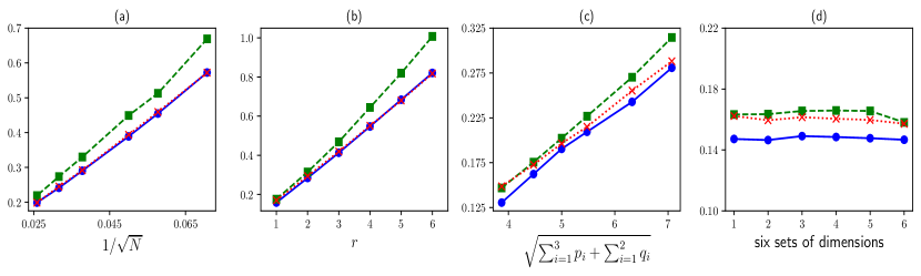
From Theorem 1, the estimation error has the convergence rate of $\sqrt{d_{\_}{\mathrm{LR}}/N}$ with $d_{\_}{\mathrm{LR}}=4r^{2}(\sum_{\_}{i=1}^{3}p_{\_}i+\sum_{\_}{i=1}^{2}q_{\_}i)+2r$, and it is proportional to $1/\sqrt{N}$, $r$ and $(\sum_{\_}{i=1}^{3}p_{\_}i+\sum_{\_}{i=1}^{2}q_{\_}i)^{1/2}$, respectively. To numerically verify them, we consider four settings: (a) $(p_{\_}i,q_{\_}j,r)$ is fixed at $(5,4,2)$ for all $i\in\{1,2,3\}$ and $j\in\{1,2\}$, while the sample size $N$ varies among the set of $\{200,300,400,700,1000,1500\}$; (b) $(p_{\_}i,q_{\_}j,N)$ is fixed at $(6,6,1000)$ for all $i\in\{1,2,3\}$ and $j\in\{1,2\}$, while the rank $r$ varies from one to six; (c) $(r,N)$ is fixed at $(1,600)$, while we use the same value for all $p_{\_}i$’s and $q_{\_}j$’s, and it varies among $\{3,4,5,6,8,10\}$; and (d) $(r,N,\sum_{\_}{i=1}^{3}p_{\_}i+\sum_{\_}{i=1}^{2}q_{\_}i)$ is fixed at $(1,600,26)$, while we vary $(p_{\_}1,p_{\_}2,p_{\_}3,q_{\_}1,q_{\_}2)$ among six different values, given in the supplementary file. Algorithm 1 with step size $\eta=0.01$ is employed to search for OLS estimators $\mbox{\boldmath$\mathscr{\widehat{A}}$}_{\_}{\mathrm{LR}}$. Estimation errors $\|\mbox{\boldmath$\mathscr{\widehat{A}}$}_{\_}{\mathrm{LR}}-\mbox{\boldmath$\mathscr{A}$}\|_{\_}{\mathrm{F}}$, averaged over 300 replications, are calculated and given in Figure 4.

The linearity in Figure 4(a)-(c) implies that $\|\mbox{\boldmath$\mathscr{\widehat{A}}$}_{\_}{\mathrm{LR}}-\mbox{\boldmath$\mathscr{A}$}\|_{\_}{\mathrm{F}}$ is proportional to $1/\sqrt{N}$, $r$, $(\sum_{\_}{i=1}^{3}p_{\_}i+\sum_{\_}{i=1}^{2}q_{\_}i)^{1/2}$, respectively, and the constancy in Figure 4(d) further verifies that the estimation error depends on dimensions only through $\sum_{\_}{i=1}^{3}p_{\_}i+\sum_{\_}{i=1}^{2}q_{\_}i$, which is one of the main advantages of tensor train regression. The theoretical findings in Theorem 1 are hence confirmed. Moreover, for the correlated data from (iii.), all estimators have a slightly worse performance, and a generalized least squares method may be needed to improve their efficiency. The finite-sample performance of OLS estimators for TT autoregression in handling time series data was also evaluated by simulation experiments, and similar findings can be observed; see the supplementary file for details.

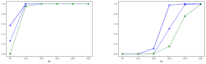
The second experiment is to evaluate the proposed rank selection methods in Section 4.2, and TT autoregression with order one at (10) is used to generate the tensor-valued time series with $d=3$ modes and $p_{\_}1=p_{\_}2=p_{\_}3=5$. The TT ranks of reshaped coefficient tensors $\mathcal{M}(\mbox{\boldmath$\mathscr{A}$})$ are set to $R=(2,2,2,2,2)$. For weight matrix $\boldsymbol{\Sigma}=\mbox{diag}\{\sigma_{\_}1,\sigma_{\_}2\}$, we consider two types of signals, $(\sigma_{\_}1,\sigma_{\_}2)=(1.5\sigma,1.5\sigma)$ and $(2\sigma,\sigma)$, with two strengths $\sigma=1$ and 2. The orthonormal matrices in the TT decomposition of $\mathcal{M}(\mbox{\boldmath$\mathscr{A}$})$ are generated as in the first experiment, and the stationarity condition in Assumption 3 is guaranteed. We set the upper bounds of ranks $\bar{r}=3$, and the sample sizes are $N=50+100j$ with $j=0,1,\cdots,5$. The BIC in Section 4.2 is conducted to select TT ranks, where the time-consuming joint rank selection procedure $\widehat{R}_{\_}{\mathrm{Joint}}$ is applied to the cases with $\sigma_{\_}{1}=\sigma_{\_}{2}$ only, while the separate rank selection procedure $\widehat{R}_{\_}{\mathrm{Separate}}$ is for all four cases.

The correct rank selection refers to the case that all five TT ranks are correctly chosen, and Figure 5 presents its proportions over 500 replications with strengths of $\sigma=1$ and 2. It can be seen that both $\widehat{R}_{\_}{\mathrm{Joint}}$ and $\widehat{R}_{\_}{\mathrm{Separate}}$ can choose the correct ranks with a higher percentage as the sample size $N$ becomes larger, and they can even correctly select the ranks for almost all 500 replications when sample size is $N=550$. The consistency in Theorem 5 is hence confirmed. Moreover, both rank selection methods perform better for stronger signals with $\sigma=2$ and, as expected, $\widehat{R}_{\_}{\mathrm{Joint}}$ has a better performance than $\widehat{R}_{\_}{\mathrm{Separate}}$ for both cases. Finally, the rank selection methods have a better performance for the cases with $\sigma_{\_}{1}=\sigma_{\_}{2}$, and we may argue that their performance is determined by the minimum strength rather than the averaged one. In fact, the minimum singular value of sequential matricization of $\mathcal{M}(\mbox{\boldmath$\mathscr{A}$})$ is $\lambda_{\_}{\mathrm{min}}=2.28$ or $1.56$ for the cases with $(\sigma_{\_}1,\sigma_{\_}2)=(3,3)$ and $(4,2)$, respectively.

5.2 Comparison to Tucker decomposition

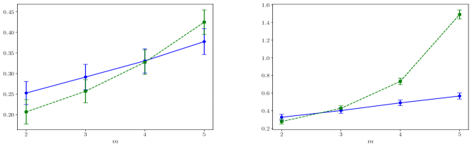
This subsection conducts a simulation experiment to compare tensor regression models with Tucker and TT decomposition. The data generating process is tensor regression model at (8) with $n=1$ and $2\leq m\leq 5$, i.e. $\boldsymbol{y}_{\_}i\in\mathbb{R}^{q_{\_}1}$ and $\mbox{\boldmath$\mathscr{X}$}_{\_}i\in\mathbb{R}^{p_{\_}1\times\cdots\times p_{\_}m}$, where $q_{\_}1=p_{\_}1=\cdots=p_{\_}m=5$, and the components of predictors $\mbox{\boldmath$\mathscr{X}$}_{\_}i$ and errors $\mbox{\boldmath$\mathscr{E}$}_{\_}i$ are independent with standard normal distribution. Note that the coefficient tensor $\mathscr{A}$ has $m+1$ modes. We first generate a coefficient tensor $\mbox{\boldmath$\mathscr{A}$}_{\_}{\mathrm{Tucker}}$ by Tucker decomposition as in (1), and all Tucker ranks are simply set to $r=2$ or 3. Orthonormal matrices, $\boldsymbol{U}_{\_}i$ with $1\leq i\leq m+1$, are generated as in the first experiment at Section 5.1, while core tensor $\mathscr{G}$ has independent entries from standard normal distribution and rescaled such that $\left\lVert\mbox{\boldmath$\mathscr{G}$}\right\rVert_{\_}{\mathrm{F}}=5$. The sample size is fixed at $N=600$. Tensor regression via Tucker decomposition (Chen et al.,, 2019) is applied to the generated samples, and a projected gradient descent algorithm is used to search for OLS estimators $\mbox{\boldmath$\mathscr{\widehat{A}}$}_{\_}{\mathrm{Tucker}}$. The averaged estimation errors $\|\mbox{\boldmath$\mathscr{\widehat{A}}$}_{\_}{\mathrm{Tucker}}-\mbox{\boldmath$\mathscr{A}$}_{\_}{\mathrm{Tucker}}\|_{\_}{\mathrm{F}}$ over 300 replications is presented in Figure 6, with one standard deviation plotted above and below the averaged value.

As a comparison, we also generate another coefficient tensor $\mbox{\boldmath$\mathscr{A}$}_{\_}{\mathrm{TT}}$ by TT decomposition as in the first experiment at Section 5.1, and all TT ranks are set to $r=2$ or 3. TT regression at Section 3.1 is applied accordingly, and Algorithm 1 is employed to search for OLS estimators $\mbox{\boldmath$\mathscr{\widehat{A}}$}_{\_}{\mathrm{TT}}$. Figure 6 also gives the averaged estimation errors $\|\mbox{\boldmath$\mathscr{\widehat{A}}$}_{\_}{\mathrm{TT}}-\mbox{\boldmath$\mathscr{A}$}_{\_}{\mathrm{TT}}\|_{\_}{\mathrm{F}}$ over 300 replications. Interestingly, as $m$ increases, estimation error $\|\mbox{\boldmath$\mathscr{\widehat{A}}$}_{\_}{\mathrm{Tucker}}-\mbox{\boldmath$\mathscr{A}$}_{\_}{\mathrm{Tucker}}\|_{\_}{\mathrm{F}}$ exhibits an exponential trend, while $\|\mbox{\boldmath$\mathscr{\widehat{A}}$}_{\_}{\mathrm{TT}}-\mbox{\boldmath$\mathscr{A}$}_{\_}{\mathrm{TT}}\|_{\_}{\mathrm{F}}$ shows a linear trend. Such difference becomes much more obvious when the ranks change a little bit from two to three. We may conclude that Tucker decomposition is only suitable for low-order tensors, while TT decomposition is preferable for high-order tensors.

6 Two empirical examples

6.1 Decoding hand trajectories from ECoG signals

Electrocorticography (ECoG) has been widely used to record brain activity for brain-machine interface (BMI) technology, and it has two categories: subdural and epidural ECoGs. The epidural ECoG is a more practical interface for real applications since it has long-term durability, and this subsection analyzes the epidural ECoG data in Shimoda et al., (2012).

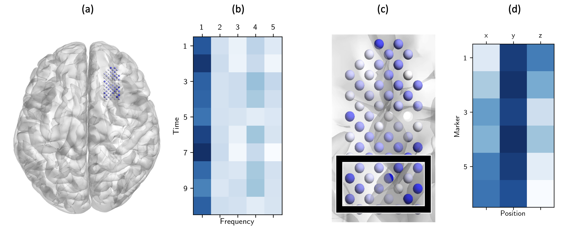
In detail, two adult Japanese monkeys were first implanted with 64-channel ECoG electrodes in the epidural space of the left hemisphere at Firgure 7(a), and they were then trained to retrieve foods using the right hand. Six markers were placed at left and right shoulder, elbow and wrist, respectively, and their 3D positions were recorded at a certain moment $i$, where the three values of a position represent the left-right, forward-backward and up-down movements, respectively. As a result, 3D positions are nested under each marker, and the hand position can be described by a matrix $\boldsymbol{Y}_{\_}i\in\mathbb{R}^{3\times 6}$. On the other hand, the ECoG signals from 64 channels were recorded with a sampling rate of 1 kHz per channel, and they were then preprocessed by the Morlet wavelet transformation at five center frequencies, 160, 80, 40, 30 and 20 Hz, where the cutoff frequencies are at 0.1 and 400 Hz; see Zhao et al., (2012). Moreover, there are ten timestamps per second, and the ECoG signals in the previous second is believed to be able to affect hand positions. Hence, a tensor is formed for predictors $\mbox{\boldmath$\mathscr{X}$}_{\_}i\in\mathbb{R}^{64\times 10\times 5}$, where the three modes represent channel, timestamp and center frequency, respectively. It has a factorial structure, and the arrangement will be explained later. We use the records for 1045 seconds on August 2, 2010, and hand position was extracted for every 0.5 second. This results in $N=2089$ observations for a regression problem $\{(\boldsymbol{Y}_{\_}i,\mbox{\boldmath$\mathscr{X}$}_{\_}i),1\leq i\leq N\}$.

Tensor regression model at (8) is applied with coefficient tensor $\mbox{\boldmath$\mathscr{A}$}\in\mathbb{R}^{3\times 6\times 64\times 10\times 5}$, and it has $57600$ parameters in total. To conduct a feasible estimation, we have to restrict $\mathscr{A}$ onto a low-dimensional space, and four dimension reduction techniques are considered. They include TT, CP and Tucker decomposition, and the fourth one is an early stopping (ES) technique in the area of machine learning (Goodfellow et al.,, 2016). Specifically, we use the gradient descent method only to update $\mbox{\boldmath$\mathscr{A}$}^{(k)}$ in Algorithm 1, while the total number of iterations are restricted to be the same as that of tensor train regression. For the sake of comparison, observations are split into two sets: the first 1500 ones for training and the last 589 for testing. We first fit TT regression to the training set, and the selected TT ranks are $R_{\_}{\mathrm{Joint}}=(2,1,3,3)$ with $\bar{r}=5$. For CP decomposition at (2), the OLS estimation is considered as in Lock, (2018), while the ridge regularization is removed. Moreover, the BIC at (17) is adapted for rank selection with $d(r)=r(\sum_{\_}{i=1}^{3}p_{\_}i+\sum_{\_}{i=1}^{2}q_{\_}i)$, $\phi=0.5$ and the upper bound of ranks $\bar{r}=5$, and the selected rank is $\widehat{r}=2$. For Tucker decomposition at (1), the OLS estimation is employed again, and the selected Tucker ranks are $\widehat{R}=(2,2,1,2,2)$ by the 95% cumulative percentage of total variation (Han et al., 2022a, ).

We next evaluate the performance of these four dimension reduction techniques on the testing set, and their $\ell_{\_}1$ and $\ell_{\_}2$ norms of forecast errors are displayed in Table 1. Specifically, the $\ell_{\_}1$ norm of forecast errors is defined as $589^{-1}\sum_{\_}{i=1}^{589}\|\operatorname*{vec}(\boldsymbol{Y}_{\_}i)-\operatorname*{vec}(\boldsymbol{\widehat{Y}}_{\_}i)\|_{\_}1$, where $\boldsymbol{\widehat{Y}}_{\_}i=\langle\mbox{\boldmath$\mathscr{\widehat{A}}$},\mbox{\boldmath$\mathscr{X}$}_{\_}i\rangle$ is the predicted value, and similarly we can define the $\ell_{\_}2$ norm of forecast errors. From Table 1, TT decomposition outperforms Tucker decomposition significantly, while it is slightly better than CP decomposition. It may be due to the facts that, for high-order tensors, Tucker decomposition fails to compress the space dramatically, while TT decomposition can reduce the parameter space as significantly as CP decomposition. Moreover, according to our experience in the model fitting, the algorithm with CP decomposition is very unstable. Finally, the ES method has the worst performance, and this is under expectation since no dimension reduction is performed.

Finally, we refit TT regression by using all observations with TT ranks $R=(2,1,3,3)$ being selected in the above, and Algorithm 2 is then employed to calculate TT decomposition, $\mbox{\boldmath$\mathscr{\widehat{A}}$}=[[\boldsymbol{G}_{\_}1,\mbox{\boldmath$\mathscr{G}$}_{\_}2,\boldsymbol{\Sigma},\mbox{\boldmath$\mathscr{G}$}_{\_}3,\mbox{\boldmath$\mathscr{G}$}_{\_}4,\boldsymbol{G}_{\_}5]]$. As a result, there are only one response factor $[\mbox{\boldmath$\mathscr{G}$}_{\_}2]_{\_}{2}^{\top}\operatorname*{vec}(\boldsymbol{G}_{\_}1^{\top}\boldsymbol{Y}_{\_}i)\in\mathbb{R}$ and one predictor factor $[\mbox{\boldmath$\mathscr{G}$}_{\_}{3}]_{\_}1([\mbox{\boldmath$\mathscr{G}$}_{\_}{4}]_{\_}1\otimes\boldsymbol{I}_{\_}{64})(\boldsymbol{G}_{\_}{5}^{\top}\otimes\boldsymbol{I}_{\_}{640})\operatorname*{vec}(\mbox{\boldmath$\mathscr{X}$}_{\_}i)\in\mathbb{R}$ in total; see Section 2.2 and (9) for details. For predictors, the orthonormal matrix $\boldsymbol{G}_{\_}5$ is first used to extract three factors from five center frequencies: the high-frequency band (or high-gamma band), low-frequency band (or beta band) and a band with mixed frequencies. We then use $\mbox{\boldmath$\mathscr{G}$}_{\_}4$ to summary all 30 factors across timestamps into three ones, one of which is obviously for high-gamma band, and finally the predictor factor can be obtained by applying $\mbox{\boldmath$\mathscr{G}$}_{\_}3$; see loading matrices in the supplementary file. To further understand how the predictor factor summarizes center frequencies and timestamps, we average the absolute loading tensor along channels, and the corresponding heatmap is presented at Figure 7(b). It can be seen that the loadings concentrate on the highest center frequency, while there is no clear trend for timestamps. This is consistent with the well known fact for ECoG that the motor behavior is highly related to the high-gamma band (Schalk et al.,, 2007; Scherer et al.,, 2009). We then focus on the high-gamma band factor from $\boldsymbol{G}_{\_}5$ and $\mbox{\boldmath$\mathscr{G}$}_{\_}4$, and the absolute loadings of its 64 channels from $\mbox{\boldmath$\mathscr{G}$}_{\_}3$ are depicted at Figure 7(c) in the term of heatmaps, where the black bounding box corresponds to primary motor cortex. Due to the importance of primary motor cortex in decoding ECoG (Shimoda et al.,, 2012), the heavy loadings on electrode channels in the black bounding box further confirm the usefulness of the proposed TT regression. For the arrangement of three modes in predictors, we placed the channel at the highest level since it is the most important to detect influential electrode channels. In the meanwhile, from the above analysis, the high-frequency band plays a key role, and hence we placed center frequencies at the lowest level such that they can be first summarized.

For the response factor, Figure 7(d) displays its heatmap of the absolute loading matrix, and six markers have roughly equal contributions to motor behavior. The forward-backward movement dominates the interpretation of hand positions, while the left-right or up-down movements have a different receptive field. It is noteworthy to point out that the fitted tensor regression via Tucker decomposition has four response and four predictor factors since the Tucker ranks are $R=(2,2,1,2,2)$, while that via CP decomposition has predictor factors only.

6.2 Australian domestic tourism flows

This subsection analyzes the Australian domestic tourism flows data, which come from the National Visitor Survey, Australia, and have been studied by Wickramasuriya et al., (2019) as a hierarchical time series. The tourism flow is measured by the total number of nights spent by Australians away from home, and three purposes of travels are considered: ”holiday”, ”visiting friends & relatives” and “business”. Four states are involved, and each has four zones; see the supplementary file for details. They forms a geographically hierarchical structure, and we consider a tensor-valued time series with the three modes corresponding to zones, states and purposes, respectively. The data were collected monthly from January 1998 to December 2016 with $N=228$ observations in total. The $\log$ transformation is first applied and, given unusual large tourism flows in every January, we then replace January’s mean by that of rest months. The resulting sequence is denoted by $\{\mbox{\boldmath$\mathscr{Y}$}_{\_}t\}$ with $\mbox{\boldmath$\mathscr{Y}$}_{\_}t\in\mathbb{R}^{4\times 4\times 3}$, and the tensor autoregression with order one at (10) has $2304$ parameters.

We consider TT autoregression with orders $p=1$ and 2 at (13), and the selected TT ranks are $\widehat{R}_{\_}{\mathrm{Joint}}=(2,2,2,2,2)$ and $(2,2,3,2,3,1)$, respectively, by using all observations. As a comparison, four commonly used methods in the literature are also considered: (i.) tensor autoregression (TAR) with order one and no restriction on the coefficient tensor, (ii.) Tucker tensor autoregression in Wang et al., 2021a with the order $p=1$ and Tucker ranks $\widehat{R}=(2,2,1,2,2,1)$ chosen by a truncation method, (iii.) multi-linear tensor autoregression (TenAR) in Li and Xiao, (2021) with the order $p=2$ and ranks $\widehat{R}=(1,1)$, both of which are selected by the extended BIC, and (iv.) tensor factor model (TFM) in Chen et al., (2022) with ranks $\widehat{R}=(1,1,1)$ by an information criterion in Han et al., 2022b . Note that there is only one factor from TFM, and hence a univariate autoregression with order one is further applied for the sake of prediction. The rolling forecast method is employed to evaluate the performance. Specifically, from January 2015, i.e. $t=205$, to December 2016, i.e. $t=228$, we keep fitting models by using the data up to time $t-1$ and then calculating the one-step-ahead forecast $\mbox{\boldmath$\mathscr{\widehat{Y}}$}_{\_}t$, and the $\ell_{\_}1$ and $\ell_{\_}2$ norms of forecast errors are given in Table 1. TT autoregression outperforms all the other four methods, and the model with order $p=2$ performs the best. Note that the TenAR method is based on CP decomposition. However, Tucker and CP decomposition, as well as factor modeling, are all for data with factorial structures, and they are not suitable for hierarchical time series.

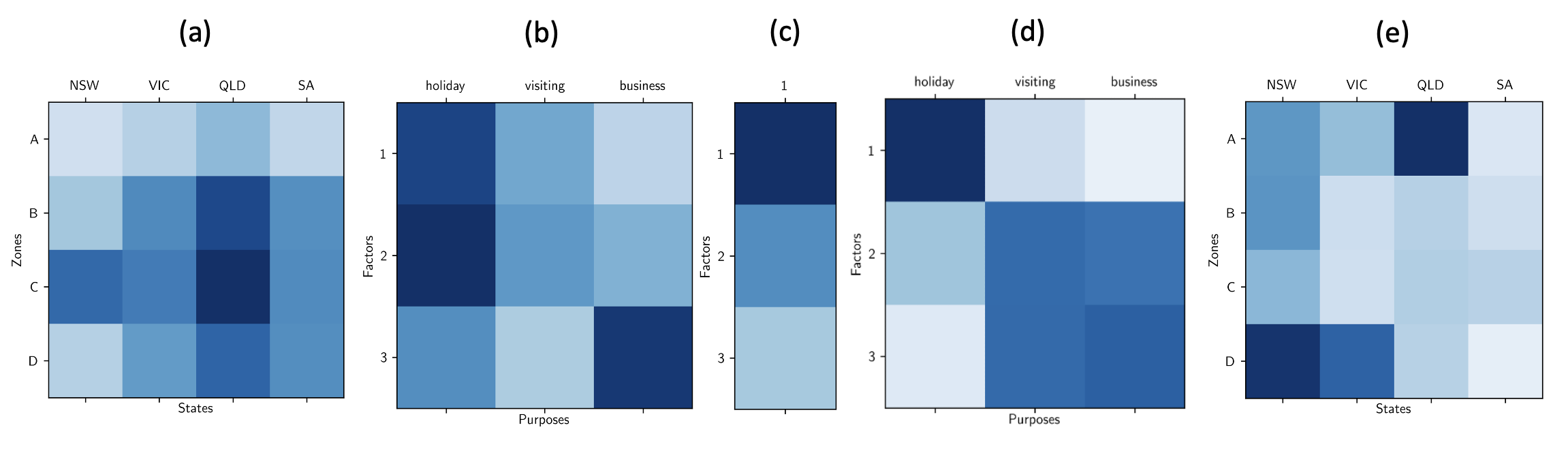
Finally, we refit the TT autoregression by using all time points with order $p=2$ and TT ranks $R=(2,2,3,2,3,1)$ selected in the above, and Algorithm 2 is then employed to calculate TT decomposition, $\mathcal{M}(\mbox{\boldmath$\mathscr{\widehat{A}}$}_{\_}{1:2})=[[\boldsymbol{G}_{\_}1,\mbox{\boldmath$\mathscr{G}$}_{\_}2,\mbox{\boldmath$\mathscr{G}$}_{\_}3,\boldsymbol{\Sigma},\mbox{\boldmath$\mathscr{G}$}_{\_}4,\mbox{\boldmath$\mathscr{G}$}_{\_}5,\mbox{\boldmath$\mathscr{G}$}_{\_}6,\boldsymbol{G}_{\_}7]]$. From Section 2.2 and (9), there are three pairs of response and predictor factors. Figure 8(a) and (e) presents the absolute loadings of zones and states from response and predictor factors, respectively, where all other modes of the loading tensors are averaged out. Note that A zone is the metro zone for each state, and their tourism flows are relatively stable, i.e. metros are not the key areas of growth (Wickramasuriya et al.,, 2019). This leads to their less contributions to the response factors in Figure 8(a). Moreover, from Figure 8(e), South Australia (SA) has less weights, and it may be due to the fact that tourism flows at SA are relatively small and hence are less powerful in driving the tourism flows of whole Australia. Thirdly, as predicted by Wickramasuriya et al., (2019), the D zone of Victoria (VIC) and B zone of Queensland (QLD) have the growth rates up to 20% in 2017, and this can be explained by the large weights in Figure 8(a). Finally, Figure 8(b) and (d) give the absolute loadings of purposes from response and predictor factors, respectively, and the diagonal elements of $\boldsymbol{\Sigma}$ are also displayed at Figure 8(c) in terms of heatmaps. It can be seen that holiday explains more variation for travel, which is consistent with the findings in Wickramasuriya et al., (2019).

7 Conclusions and discussions

This paper proposes a new tenor regression, tensor train (TT) regression, by revising the classical TT decomposition and then applying it to the coefficient tensor, and the new model is further extended to TT autoregression in handling time series data. Comparing with the models via Tucker decomposition, the two new models can be applied to the case with higher order responses and predictors, while they have the same stable numerical performance. Moreover, the proposed new models are shown to well match the data with hierarchical structures, and they also have better interpretation even for factorial data, which are supposed to be better fitted by Tucker decomposition.

The proposed methodology in this paper can be extended along three directions. First, for TT regression, the sample size is required to be $N\gtrsim\sum_{\_}{i=1}^{m}p_{\_}i+\sum_{\_}{i=1}^{n}q_{\_}i$ such that the estimation consistency can be obtained, while the number of variables for some modes may be larger than the sample size $N$ in some real applications. To handle this case, we may further impose sparsity to the components of TT decomposition (Basu and Michailidis,, 2015; Wang et al., 2021b, ). Specifically, for the coefficient tensor $\mbox{\boldmath$\mathscr{A}$}=[[\boldsymbol{G}_{\_}1,\mbox{\boldmath$\mathscr{G}$}_{\_}2,\cdots,\boldsymbol{\Sigma},\cdots,\mbox{\boldmath$\mathscr{G}$}_{\_}{m+n-1},\boldsymbol{G}_{\_}{m+n}]]$ with TT ranks $(r_{\_}1,\ldots,r_{\_}{m+n-1})$, let $s_{\_}1$ and $s_{\_}{m+n}$ be the number of non-zero rows of $\boldsymbol{G}_{\_}1\in\mathbb{R}^{q_{\_}1\times r_{\_}1}$ and $\boldsymbol{G}_{\_}{m+n}\in\mathbb{R}^{q_{\_}{m+n}\times r_{\_}{m+n-1}}$, respectively, and $s_{\_}k$ be the number of non-zero lateral slices of $\mbox{\boldmath$\mathscr{G}$}_{\_}k\in\mathbb{R}^{r_{\_}{k-1}\times q_{\_}k\times r_{\_}k}$ with $2\leq k\leq m+n-1$, where $q_{\_}{n+j}=p_{\_}j$ for $1\leq j\leq m$. Note that $1\leq s_{\_}k\leq q_{\_}k$ for $1\leq k\leq m+n$, and we can conduct estimation by a hard thresholding method. Denote by $\mbox{\boldmath$\mathscr{\widehat{A}}$}_{\_}{\mathrm{SP}}$ the corresponding estimator, and it can be verified that $\|\mbox{\boldmath$\mathscr{\widehat{A}}$}_{\_}{\mathrm{SP}}-\mbox{\boldmath$\mathscr{A}$}^{*}\|_{\_}{\mathrm{F}}\lesssim\sqrt{s_{\_}{\max}(r_{\_}{\max}^{2}+\sum_{\_}{i=1}^{m}\log p_{\_}i+\sum_{\_}{i=1}^{n}\log q_{\_}i)/N}$ with high probability, where $s_{\_}{\max}=\mathrm{max}\{s_{\_}1,s_{\_}2,\cdots,s_{\_}{m+n}\}$, and the required sample size is significantly reduced. The algorithms in Section 4 can also be adopted to search for estimators. Secondly, the currently used factor modeling methods for tensor-valued time series are all based on Tucker decomposition (Chen et al.,, 2022; Wang et al.,, 2019) and, as mentioned in Section 2.2, they cannot be used for the data with hierarchical structures. It is of interest to use TT decomposition for factor modeling. Finally, when solving the optimization problems, the alternating method is well known to be faster than the projected one since no singular value decomposition is involved (Zhang and Xia,, 2018), and we may also consider an alternating least squares method (Han et al., 2022a, ) to search for the estimators in this paper. However, it is more difficult to discuss the convergence analysis for TT decomposition, and we leave it for future research.

References

  • Basu and Michailidis, (2015) Basu, S. and Michailidis, G. (2015). Regularized estimation in sparse high-dimensional time series models. The Annals of Statistics, 43:1535–1567.
  • Bi et al., (2018) Bi, X., Qu, A., and Shen, X. (2018). Multilayer tensor factorization with applications to recommender systems. The Annals of Statistics, 46:3308–3333.
  • Bravyi et al., (2021) Bravyi, S., Gosset, D., and Movassagh, R. (2021). Classical algorithms for quantum mean values. Nature Physics, 17:337–341.
  • Candes and Plan, (2011) Candes, E. J. and Plan, Y. (2011). Tight oracle inequalities for low-rank matrix recovery from a minimal number of noisy random measurements. IEEE Transactions on Information Theory, 57:2342–2359.
  • Chen et al., (2019) Chen, H., Raskutti, G., and Yuan, M. (2019). Non-convex projected gradient descent for generalized low-rank tensor regression. Journal of Machine Learning Research, 20:172–208.
  • Chen et al., (2021) Chen, R., Xiao, H., and Yang, D. (2021). Autoregressive models for matrix-valued time series. Journal of Econometrics, 222:539–560.
  • Chen et al., (2022) Chen, R., Yang, D., and Zhang, C.-H. (2022). Factor models for high-dimensional tensor time series. Journal of the American Statistical Association, 117:94–116.
  • Cichocki et al., (2015) Cichocki, A., Mandic, D., De Lathauwer, L., Zhou, G., Zhao, Q., Caiafa, C., and Phan, H. A. (2015). Tensor decompositions for signal processing applications: from two-way to multiway component analysis. IEEE Signal Processing Magazine, 32:145–163.
  • De Lathauwer et al., (2000) De Lathauwer, L., De Moor, B., and Vandewalle, J. (2000). On the best rank-1 and rank-($r_{\_}1$, $r_{\_}2$,…, $r_{\_}n$) approximation of higher-order tensors. SIAM Journal on Matrix Analysis and Applications, 21:1324–1342.
  • Gahrooei et al., (2021) Gahrooei, M. R., Yan, H., Paynabar, K., and Shi, J. (2021). Multiple tensor-on-tensor regression: an approach for modeling processes with heterogeneous sources of data. Technometrics, 63:147–159.
  • Goodfellow et al., (2016) Goodfellow, I. J., Bengio, Y., and Courville, A. (2016). Deep Learning. MIT Press, Cambridge.
  • (12) Han, R., Willett, R., and Zhang, A. (2022a). An optimal statistical and computational framework for generalized tensor estimation. The Annals of Statistics, 50:1–29.
  • (13) Han, Y., Chen, R., and Zhang, C.-H. (2022b). Rank determination in tensor factor model. Electronic Journal of Statistics, 16:1726–1803.
  • Hao et al., (2021) Hao, B., Wang, B., Wang, P., Zhang, J., Yang, J., and Sun, W. W. (2021). Sparse tensor additive regression. Journal of Machine Learning Research, 22:1–43.
  • Harshman, (1970) Harshman, R. A. (1970). Foundations of the PARAFAC procedure: models and conditions for an ”explanatory” multimodal factor analysis. UCLA Working Papers in Phonetics, 16:1–84.
  • Hillar and Lim, (2013) Hillar, C. J. and Lim, L.-H. (2013). Most tensor problems are NP-hard. Journal of the ACM, 60:1–39.
  • Jain et al., (2014) Jain, P., Tewari, A., and Kar, P. (2014). On iterative hard thresholding methods for high-dimensional m-estimation. Advances in neural information processing systems, 27.
  • Kim et al., (2019) Kim, T., Lee, J., and Choe, Y. (2019). Tensor train decomposition for efficient memory saving in perceptual feature-maps. In Proceedings of the IEEE/CVF International Conference on Computer Vision Workshops, pages 599–604.
  • Kolda and Bader, (2009) Kolda, T. G. and Bader, B. W. (2009). Tensor decompositions and applications. SIAM Review, 51:455–500.
  • Kossaifi et al., (2020) Kossaifi, J., Lipton, Z. C., Kolbeinsson, A., Khanna, A., Furlanello, T., and Anandkumar, A. (2020). Tensor regression networks. Journal of Machine Learning Research, 21:1–21.
  • Li et al., (2018) Li, X., Xu, D., Zhou, H., and Li, L. (2018). Tucker tensor regression and neuroimaging analysis. Statistics in Biosciences, 10:520–545.
  • Li and Xiao, (2021) Li, Z. and Xiao, H. (2021). Multi-linear tensor autoregressive models. arXiv preprint arXiv:2110.00928.
  • Liu et al., (2020) Liu, Y., Liu, J., and Zhu, C. (2020). Low-rank tensor train coefficient array estimation for tensor-on-tensor regression. IEEE Transactions on Neural Networks and Learning Systems, 31:5402–5411.
  • Lock, (2018) Lock, E. F. (2018). Tensor-on-tensor regression. Journal of Computational and Graphical Statistics, 27:638–647.
  • Luo and Zhang, (2022) Luo, Y. and Zhang, A. R. (2022). Tensor clustering with planted structures: statistical optimality and computational limits. The Annals of Statistics, 50:584–613.
  • Montgomery, (2006) Montgomery, D. C. (2006). Design and Analysis of Experiments. John Wiley & Sons, Inc., Hoboken.
  • Novikov et al., (2015) Novikov, A., Podoprikhin, D., Osokin, A., and Vetrov, D. P. (2015). Tensorizing neural networks. Advances in neural information processing systems, 28.
  • Orús, (2019) Orús, R. (2019). Tensor networks for complex quantum systems. Nature Reviews Physics, 1:538–550.
  • Oseledets and Tyrtyshnikov, (2010) Oseledets, I. and Tyrtyshnikov, E. (2010). TT-cross approximation for multidimensional arrays. Linear Algebra and its Applications, 432:70–88.
  • Oseledets, (2011) Oseledets, I. V. (2011). Tensor-train decomposition. SIAM Journal on Scientific Computing, 33:2295–2317.
  • Raskutti et al., (2019) Raskutti, G., Yuan, M., and Chen, H. (2019). Convex regularization for high-dimensional multiresponse tensor regression. The Annals of Statistics, 47:1554–1584.
  • Rigollet, (2015) Rigollet, P. (2015). High dimensional statistics. Massachusetts Institute of Technology: MIT OpenCourseWare, https://ocw.mit.edu.
  • Schalk et al., (2007) Schalk, G., Kubanek, J., Miller, K. J., Anderson, N., Leuthardt, E. C., Ojemann, J. G., Limbrick, D., Moran, D., Gerhardt, L. A., and Wolpaw, J. R. (2007). Decoding two-dimensional movement trajectories using electrocorticographic signals in humans. Journal of Neural Engineering, 4:264.
  • Scherer et al., (2009) Scherer, R., Zanos, S. P., Miller, K. J., Rao, R. P., and Ojemann, J. G. (2009). Classification of contralateral and ipsilateral finger movements for electrocorticographic brain-computer interfaces. Neurosurgical Focus, 27:E12.
  • Shimoda et al., (2012) Shimoda, K., Nagasaka, Y., Chao, Z. C., and Fujii, N. (2012). Decoding continuous three-dimensional hand trajectories from epidural electrocorticographic signals in japanese macaques. Journal of Neural Engineering, 9:036015.
  • Su et al., (2020) Su, J., Byeon, W., Kossaifi, J., Huang, F., Kautz, J., and Anandkumar, A. (2020). Convolutional tensor-train lstm for spatio-temporal learning. Advances in Neural Information Processing Systems, 33:13714–13726.
  • Sun and Li, (2019) Sun, W. W. and Li, L. (2019). Dynamic tensor clustering. Journal of the American Statistical Association, 114:1894–1907.
  • Tucker, (1966) Tucker, L. R. (1966). Some mathematical notes on three-mode factor analysis. Psychometrika, 31:279–311.
  • Wainwright, (2019) Wainwright, M. J. (2019). High-Dimensional Statistics: A Non-Asymptotic Viewpoint. Cambridge University Press, Cambridge.
  • Wang et al., (2019) Wang, D., Liu, X., and Chen, R. (2019). Factor models for matrix-valued high-dimensional time series. Journal of Econometrics, 208:231–248.
  • (41) Wang, D., Zheng, Y., and Li, G. (2021a). High-dimensional low-rank tensor autoregressive time series modeling. arXiv preprint arXiv:2101.04276.
  • (42) Wang, D., Zheng, Y., Lian, H., and Li, G. (2021b). High-dimensional vector autoregressive time series modeling via tensor decomposition. Journal of the American Statistical Association. To appear.
  • Wickramasuriya et al., (2019) Wickramasuriya, S. L., Athanasopoulos, G., and Hyndman, R. J. (2019). Optimal forecast reconciliation for hierarchical and grouped time series through trace minimization. Journal of the American Statistical Association, 114:804–819.
  • Yang et al., (2017) Yang, Y., Krompass, D., and Tresp, V. (2017). Tensor-train recurrent neural networks for video classification. In International Conference on Machine Learning, pages 3891–3900. PMLR.
  • Zhang and Xia, (2018) Zhang, A. and Xia, D. (2018). Tensor SVD: Statistical and computational limits. IEEE Transactions on Information Theory, 64:7311–7338.
  • Zhang and Ng, (2022) Zhang, X. and Ng, M. K. (2022). Robust tensor train component analysis. Numerical Linear Algebra with Applications, 29:e2403.
  • Zhao et al., (2012) Zhao, Q., Caiafa, C. F., Mandic, D. P., Chao, Z. C., Nagasaka, Y., Fujii, N., Zhang, L., and Cichocki, A. (2012). Higher order partial least squares (HOPLS): a generalized multilinear regression method. IEEE Transactions on Pattern Analysis and Machine Intelligence, 35:1660–1673.
  • Zhou et al., (2013) Zhou, H., Li, L., and Zhu, H. (2013). Tensor regression with applications in neuroimaging data analysis. Journal of the American Statistical Association, 108:540–552.
  • Zhou et al., (2022) Zhou, Y., Zhang, A. R., Zheng, L., and Wang, Y. (2022). Optimal high-order tensor svd via tensor-train orthogonal iteration. IEEE Transactions on Information Theory. To appear.
Refer to caption
Figure 3: Heatmaps of loading matrices from one response factor by TT decomposition and four by Tucker decomposition. Six countries consists of USA, United Kingdom (GBR), Spain (ESP), Belgium (BEL), Australia (AUS) and Brazil (BRA).
Refer to caption
Figure 4: Averaged estimation errors $\|\mbox{\boldmath$\mathscr{\widehat{A}}$}_{\_}{\mathrm{LR}}-\mbox{\boldmath$\mathscr{A}$}\|_{\_}{\mathrm{F}}$ for tensor train regression under Settings (a)-(d). Predictors and errors are independent with uniform distribution ( ), independent with normality ( ) or correlated with normality ( ).
Refer to caption
Figure 5: Proportions of correct rank selection for the data with stronger (left panel) and weaker (right panel) signals, corresponding to $\sigma=2$ and 1, respectively. We consider the joint selection procedure $\widehat{R}_{\_}{\mathrm{Joint}}$ for the case with $\sigma_{\_}{1}=\sigma_{\_}{2}$ ( ), and separate selection procedure $\widehat{R}_{\_}{\mathrm{Separate}}$ for the cases with $\sigma_{\_}{1}=\sigma_{\_}{2}$ ( ) and $\sigma_{\_}{1}\neq\sigma_{\_}{2}$ ( ).
Refer to caption
Figure 6: Averaged estimation errors $\|\mbox{\boldmath$\mathscr{\widehat{A}}$}-\mbox{\boldmath$\mathscr{A}$}\|_{\_}{\mathrm{F}}$ for tensor regression via Tucker ( ) and TT ( ) decomposition with ranks being $r=2$ (left panel) or 3 (right panel). One standard deviation is plotted above and below the averaged value.
Table 1: $\ell_{\_}1$ and $\ell_{\_}2$ norms of forecasting errors for the epidural ECoG and Australian tourism flows examples in Sections 6.1 and 6.2, respectively.
ECoG example Tourism flows example
Criterion TT CP Tucker ES TT-1 TT-2 TAR Tucker TenAR TFM
$\ell_{\_}1$ norm 12.97 12.97 15.32 15.40 16.60 16.41 17.76 17.64 16.74 17.88
$\ell_{\_}2$ norm 3.41 3.42 3.99 4.07 3.35 3.32 3.65 3.56 3.37 3.59
Refer to caption
(a)
Figure 7: Four plots from the ECoG example: (a) location the epidural space (blue area), (b) heatmap of absolute loadings on timestamps and center frequencies for the predictor factor with the mode of channels being averaged, (c) absolute loadings on 64 electrode channels for the high-frequency band factor from $\boldsymbol{G}_{\_}5$ and $\mbox{\boldmath$\mathscr{G}$}_{\_}4$, and (d) heatmap of the absolute loading matrix for the response factor. Larger values are presented with darker colors, and the black bounding box at (c) corresponds to the primary motor cortex (Shimoda et al.,, 2012).
Refer to caption
Figure 8: Five heatmaps from the Tourism flows example: (a) absolute loadings of zones and states from response factors, (b) absolute loadings of purposes from three response factors, (c) regression coefficients of response factors on predictor ones, i.e. the diagonal elements of $\boldsymbol{\Sigma}$, (d) absolute loadings of purposes from three predictor factors, and (e) absolute loadings of states and zones from predictor factors. All other modes of loading tensors are averaged out.

A Technical proofs of propositions and theorems

Section A.1 gives the technical proofs of Proposition 1 and Theorems 1-5, which depend on five auxiliary lemmas in Section A.2.

A.1 Proofs of Proposition 1 and Theorems 1-5

Proof of Proposition 1..

We first discuss the identification problem of tensor train decomposition. If $\mathscr{X}$ has TT-cores $\boldsymbol{G}_{\_}1,\mbox{\boldmath$\mathscr{G}$}_{\_}2\cdots\mbox{\boldmath$\mathscr{G}$}_{\_}{d-1},\boldsymbol{G}_{\_}d$, by Lemma 3.1 in Zhou et al., (2022), for $1\leq k\leq d-1$,

$$[\mbox{\boldmath$\mathscr{X}$}]_{\_}k=(\boldsymbol{I}_{\_}{p_{\_}2\cdots p_{\_}k}\otimes\boldsymbol{G}_{\_}1)\cdots(\boldsymbol{I}_{\_}{p_{\_}k}\otimes[\mbox{\boldmath$\mathscr{G}$}_{\_}{k-1}]_{\_}2)[\mbox{\boldmath$\mathscr{G}$}_{\_}k]_{\_}2[\mbox{\boldmath$\mathscr{G}$}_{\_}{k+1}]_{\_}1([\mbox{\boldmath$\mathscr{G}$}_{\_}{k+2}]_{\_}1\otimes\boldsymbol{I}_{\_}{p_{\_}{k+1}})\cdots(\boldsymbol{G}_{\_}{d}^{\top}\otimes\boldsymbol{I}_{\_}{p_{\_}{k+1}\cdots p_{\_}{d-1}}).$$

Note that given nonsingular matrices $\boldsymbol{O}_{\_}i\in\mathbb{R}^{r_{\_}{i}\times r_{\_}i}$ for $1\leq i\leq d-1$. Since

$\displaystyle[\mbox{\boldmath$\mathscr{X}$}]_{\_}1$ $\displaystyle=\boldsymbol{G}_{\_}1[\mbox{\boldmath$\mathscr{G}$}_{\_}2]_{\_}1([\mbox{\boldmath$\mathscr{G}$}_{\_}3]_{\_}1\otimes\boldsymbol{I}_{\_}{p_{\_}2})\cdots(\boldsymbol{G}_{\_}{d}^{\top}\otimes\boldsymbol{I}_{\_}{p_{\_}{2}\cdots p_{\_}{d-1}})$
$\displaystyle=\boldsymbol{G}_{\_}1\boldsymbol{O}_{\_}1\boldsymbol{O}_{\_}1^{-1}[\mbox{\boldmath$\mathscr{G}$}_{\_}2]_{\_}1([\mbox{\boldmath$\mathscr{G}$}_{\_}3]_{\_}1\otimes\boldsymbol{I}_{\_}{p_{\_}2})\cdots(\boldsymbol{G}_{\_}{d}^{\top}\otimes\boldsymbol{I}_{\_}{p_{\_}{2}\cdots p_{\_}{d-1}}),$

the tensor $\mathscr{X}$ could also be decomposed to $\boldsymbol{G}_{\_}1\boldsymbol{O}_{\_}1,\mbox{\boldmath$\mathscr{G}$}_{\_}2\times_{\_}1\boldsymbol{O}_{\_}1^{-1},\mbox{\boldmath$\mathscr{G}$}_{\_}3\cdots\mbox{\boldmath$\mathscr{G}$}_{\_}{d-1},\boldsymbol{G}_{\_}d$. Sequentially matricize $\mathscr{X}$ to $[\mbox{\boldmath$\mathscr{X}$}]_{\_}{2},\cdots,[\mbox{\boldmath$\mathscr{X}$}]_{\_}{d-1}$ and repeatly apply Lemma 3.1 in Zhou et al., (2022), we can see that $\mathscr{X}$ can also decomposed to $\boldsymbol{G}_{\_}1\boldsymbol{O}_{\_}1,\mbox{\boldmath$\mathscr{G}$}_{\_}2\times_{\_}1\boldsymbol{O}_{\_}1^{-1}\times_{\_}3\boldsymbol{O}_{\_}2^{\top}\cdots\mbox{\boldmath$\mathscr{G}$}_{\_}{d-1}\times_{\_}1\boldsymbol{O}_{\_}{d-2}^{-1}\times_{\_}3\boldsymbol{O}_{\_}{d-1}^{\top},\boldsymbol{O}_{\_}{d-1}^{-1}\boldsymbol{G}_{\_}d$.

To fix the decomposition, by applying Algorithm 2, we can get orthonormal cores $[\mbox{\boldmath$\mathscr{G}$}_{\_}i]_{\_}2^{\top}[\mbox{\boldmath$\mathscr{G}$}_{\_}i]_{\_}2=\boldsymbol{I}_{\_}{r_{\_}i}$ for $2\leq i\leq k$, $[\mbox{\boldmath$\mathscr{G}$}_{\_}i]_{\_}1[\mbox{\boldmath$\mathscr{G}$}_{\_}i]_{\_}1^{\top}=\boldsymbol{I}_{\_}{r_{\_}{i-1}}$ for $k+1\leq i\leq d-1$, $\boldsymbol{G}_{\_}1^{\top}\boldsymbol{G}_{\_}1=\boldsymbol{I}_{\_}{r_{\_}1}$ and $\boldsymbol{G}_{\_}d\boldsymbol{G}_{\_}d^{\top}=\boldsymbol{I}_{\_}{r_{\_}{d-1}}$. As a result, $\boldsymbol{\Sigma}\in\mathbb{R}^{r_{\_}k\times r_{\_}k}$ is a diagonal matrix. It produces a unique Tensor Train decomposition, for which the $k$th sequential matricization could be expressed as

$$[\mbox{\boldmath$\mathscr{X}$}]_{\_}k=(\boldsymbol{I}_{\_}{p_{\_}2\cdots p_{\_}k}\otimes\boldsymbol{G}_{\_}1)\cdots(\boldsymbol{I}_{\_}{p_{\_}k}\otimes[\mbox{\boldmath$\mathscr{G}$}_{\_}{k-1}]_{\_}2)[\mbox{\boldmath$\mathscr{G}$}_{\_}k]_{\_}2\boldsymbol{\Sigma}[\mbox{\boldmath$\mathscr{G}$}_{\_}{k+1}]_{\_}1([\mbox{\boldmath$\mathscr{G}$}_{\_}{k+2}]_{\_}1\otimes\boldsymbol{I}_{\_}{p_{\_}{k+1}})\cdots(\boldsymbol{G}_{\_}{d}^{\top}\otimes\boldsymbol{I}_{\_}{p_{\_}{k+1}\cdots p_{\_}{d-1}}).$$

Proof of Theorem 1..

Denote sets ${\mathcal{S}}_{\_}R=\{\mbox{\boldmath$\mathscr{A}$}\in\mathbb{R}^{q_{\_}{1}\times\cdots\times q_{\_}{n}\times p_{\_}{1}\times\cdots p_{\_}{m}}:\mbox{\boldmath$\mathscr{A}$}(i_{\_}1,\cdots,i_{\_}{n+m})$ $=\boldsymbol{G}_{\_}1{(i_{\_}1)}\boldsymbol{G}_{\_}2{(i_{\_}2)}\cdots\boldsymbol{G}_{\_}{n+m}{(i_{\_}{n+m})}:\boldsymbol{G}_{\_}k{(i_{\_}k)}\in\mathbb{R}^{r_{\_}{k-1}\times r_{\_}k}$ for $k=1,2,\cdots,n+m\}$ and $\mathcal{S}_{\_}R^{\prime}=\{\mbox{\boldmath$\mathscr{A}$}\in{\mathcal{S}}_{\_}R:\|\mbox{\boldmath$\mathscr{A}$}\|_{\_}{\mathrm{F}}=1\}$, where $R=(r_{\_}0,r_{\_}1,\cdots,r_{\_}n,\cdots,r_{\_}{n+m})$ with $r_{\_}0=r_{\_}{n+m}=1$, and $r_{\_}{\mathrm{max}}=\mathrm{max}\{r_{\_}1,r_{\_}2,\cdots,r_{\_}{n+m-1}\}$. The quadratic loss function could be shown as

$$L(\mbox{\boldmath$\mathscr{A}$})=\frac{1}{N}\sum_{\_}{i=1}^{N}\left\lVert\mbox{\boldmath$\mathscr{Y}$}_{\_}i-\langle\mbox{\boldmath$\mathscr{A}$},\mbox{\boldmath$\mathscr{X}$}_{\_}{i}\rangle\right\rVert_{\_}{\mathrm{F}}^{2}=\frac{1}{N}\sum_{\_}{i=1}^{N}\left\lVert\operatorname*{vec}{(\mbox{\boldmath$\mathscr{Y}$}_{\_}i)}-[\mbox{\boldmath$\mathscr{A}$}]_{\_}{n}\operatorname*{vec}{(\mbox{\boldmath$\mathscr{X}$}_{\_}{i})}\right\rVert_{\_}2^{2}.$$

Denote $\boldsymbol{y}_{\_}i=\operatorname*{vec}(\mbox{\boldmath$\mathscr{Y}$}_{\_}i)$, $\boldsymbol{x}_{\_}i=\operatorname*{vec}(\mbox{\boldmath$\mathscr{X}$}_{\_}i)$ and $\boldsymbol{e}_{\_}i=\operatorname*{vec}(\mbox{\boldmath$\mathscr{E}$}_{\_}i)$. By the optimality of $\mbox{\boldmath$\mathscr{\widehat{A}}$}_{\_}{\mathrm{LR}}$, we have

$\displaystyle\frac{1}{N}\sum_{\_}{i=1}^{N}\left\lVert\boldsymbol{y}_{\_}i-[\mbox{\boldmath$\mathscr{\widehat{A}}$}_{\_}{\mathrm{LR}}]_{\_}n\boldsymbol{x}_{\_}{i}\right\rVert_{\_}2^{2}\leq\frac{1}{N}\sum_{\_}{i=1}^{N}\left\lVert\boldsymbol{y}_{\_}i-[\mbox{\boldmath$\mathscr{A}$}^{\ast}]_{\_}{n}\boldsymbol{x}_{\_}{i}\right\rVert_{\_}2^{2}$
$\displaystyle\Rightarrow$ $\displaystyle\frac{1}{N}\sum_{\_}{i=1}^{N}\left\lVert[\boldsymbol{\Delta}]_{\_}{n}\boldsymbol{x}_{\_}{i}\right\rVert_{\_}2^{2}\leq\frac{2}{N}\sum_{\_}{i=1}^{N}\langle\boldsymbol{e}_{\_}i,[\boldsymbol{\Delta}]_{\_}{n}\boldsymbol{x}_{\_}{i}\rangle$
$\displaystyle\Rightarrow$ $\displaystyle\frac{1}{N}\sum_{\_}{i=1}^{N}\left\lVert[\boldsymbol{\Delta}]_{\_}{n}\boldsymbol{x}_{\_}{i}\right\rVert_{\_}2^{2}\leq 2\langle\frac{1}{N}\sum_{\_}{i=1}^{N}\mbox{\boldmath$\mathscr{E}$}_{\_}{i}\circ\mbox{\boldmath$\mathscr{X}$}_{\_}i,\boldsymbol{\Delta}\rangle$
$\displaystyle\Rightarrow$ $\displaystyle\frac{1}{N}\sum_{\_}{i=1}^{N}\left\lVert[\boldsymbol{\Delta}]_{\_}{n}\boldsymbol{x}_{\_}{i}\right\rVert_{\_}2^{2}\leq 2\left\lVert\boldsymbol{\Delta}\right\rVert_{\_}{\mathrm{F}}\sup_{\_}{\boldsymbol{\Delta}\in\mathcal{S}_{\_}{2R}^{\prime}}\langle\frac{1}{N}\sum_{\_}{i=1}^{N}\mbox{\boldmath$\mathscr{E}$}_{\_}{i}\circ\mbox{\boldmath$\mathscr{X}$}_{\_}i,\boldsymbol{\Delta}\rangle,$ (A.1)

where $\boldsymbol{\Delta}=\mbox{\boldmath$\mathscr{\widehat{A}}$}_{\_}{\mathrm{LR}}-\mbox{\boldmath$\mathscr{A}$}^{\ast}\in{\mathcal{S}}_{\_}{2R}$ since $\mbox{\boldmath$\mathscr{A}$}^{\ast},\mbox{\boldmath$\mathscr{\widehat{A}}$}_{\_}{\mathrm{LR}}\in{\mathcal{S}}_{\_}R$ and the outer product of two tensors $\mbox{\boldmath$\mathscr{X}$}\in\mathbb{R}^{p_{\_}{1}\times\cdots\times p_{\_}{m}}$ and $\mbox{\boldmath$\mathscr{Y}$}\in\mathbb{R}^{q_{\_}{1}\times\cdots\times q_{\_}{n}}$ is defined as $(\mbox{\boldmath$\mathscr{X}$}\circ\mbox{\boldmath$\mathscr{Y}$})\in\mathbb{R}^{p_{\_}{1}\times\cdots p_{\_}{m}\times q_{\_}{1}\times\cdots q_{\_}{n}}$ where

$$(\mbox{\boldmath$\mathscr{X}$}\circ\mbox{\boldmath$\mathscr{Y}$})_{\_}{i_{\_}{1}\ldots i_{\_}{m+n}}=\mbox{\boldmath$\mathscr{X}$}_{\_}{i_{\_}{1}\ldots i_{\_}{m}}\mbox{\boldmath$\mathscr{Y}$}_{\_}{i_{\_}{m+1}\ldots i_{\_}{m+n}}.$$

Consider a $\epsilon$-net $\bar{\mathcal{S}}_{\_}{2R}$ with the cardinality of $\mathcal{N}(2R,\epsilon)$ for $\mathcal{S}_{\_}{2R}^{\prime}$. For any $\boldsymbol{\Delta}\in\mathcal{S}_{\_}{2R}^{\prime}$, there exists a $\bar{\boldsymbol{\Delta}}_{\_}k\in\bar{\mathcal{S}}_{\_}{2R}$ such that $\left\lVert\boldsymbol{\Delta}-\bar{\boldsymbol{\Delta}}_{\_}k\right\rVert_{\_}{\mathrm{F}}\leq\epsilon$. Since the rank of ${\boldsymbol{\Delta}-\bar{\boldsymbol{\Delta}}_{\_}k}$ is not contrained up to $2R$, we introduce the following decomposition. From Lemma 1(a), there exists $\boldsymbol{\Delta}_{\_}1,\boldsymbol{\Delta}_{\_}2,\cdots,\boldsymbol{\Delta}_{\_}{2^{m+n-1}}\in\mathcal{S}_{\_}{2R}$ such that $\boldsymbol{\Delta}-\bar{\boldsymbol{\Delta}}_{\_}k=\boldsymbol{\Delta}_{\_}1+\boldsymbol{\Delta}_{\_}2+\cdots+\boldsymbol{\Delta}_{\_}{2^{m+n-1}}$ and $\langle\boldsymbol{\Delta}_{\_}s,\boldsymbol{\Delta}_{\_}l\rangle=0$ for $s,l=1,2,\cdots,2^{m+n-1}$, $s\neq l$. By Cauchy-Schwarz inequality, $\left\lVert\boldsymbol{\Delta}_{\_}1\right\rVert_{\_}{\mathrm{F}}+\left\lVert\boldsymbol{\Delta}_{\_}2\right\rVert_{\_}{\mathrm{F}}+\cdots+\left\lVert\boldsymbol{\Delta}_{\_}{2^{m+n-1}}\right\rVert_{\_}{\mathrm{F}}\leq 2^{\frac{m+n-1}{2}}\left\lVert\boldsymbol{\Delta}-\bar{\boldsymbol{\Delta}}_{\_}k\right\rVert_{\_}{\mathrm{F}}<2^{\frac{m+n}{2}}\epsilon$ since $\left\lVert\boldsymbol{\Delta}-\bar{\boldsymbol{\Delta}}_{\_}k\right\rVert_{\_}{\mathrm{F}}^{2}=\left\lVert\boldsymbol{\Delta}_{\_}1\right\rVert_{\_}{\mathrm{F}}^{2}+\left\lVert\boldsymbol{\Delta}_{\_}2\right\rVert_{\_}{\mathrm{F}}^{2}+\cdots+\left\lVert\boldsymbol{\Delta}_{\_}{2^{m+n-1}}\right\rVert_{\_}{\mathrm{F}}^{2}$. Hence for any $\boldsymbol{\Delta}\in\mathcal{S}_{\_}{2R}^{\prime}$, we have

$\displaystyle\langle\frac{1}{N}\sum_{\_}{i=1}^{N}\mbox{\boldmath$\mathscr{E}$}_{\_}{i}\circ\mbox{\boldmath$\mathscr{X}$}_{\_}i,\boldsymbol{\Delta}\rangle\leq\max_{\_}{1\leq k\leq\mathcal{N}(2R,\epsilon)}\langle\frac{1}{N}\sum_{\_}{i=1}^{N}\mbox{\boldmath$\mathscr{E}$}_{\_}{i}\circ\mbox{\boldmath$\mathscr{X}$}_{\_}i,\bar{\boldsymbol{\Delta}}_{\_}k\rangle+2^{\frac{m+n}{2}}\epsilon\sup_{\_}{\boldsymbol{\Delta}\in\mathcal{S}_{\_}{2R}^{\prime}}\langle\frac{1}{N}\sum_{\_}{i=1}^{N}\mbox{\boldmath$\mathscr{E}$}_{\_}{i}\circ\mbox{\boldmath$\mathscr{X}$}_{\_}i,\boldsymbol{\Delta}\rangle,$
$\displaystyle\sup_{\_}{\boldsymbol{\Delta}\in\mathcal{S}_{\_}{2R}^{\prime}}\langle\frac{1}{N}\sum_{\_}{i=1}^{N}\mbox{\boldmath$\mathscr{E}$}_{\_}{i}\circ\mbox{\boldmath$\mathscr{X}$}_{\_}i,\boldsymbol{\Delta}\rangle\leq(1-2^{\frac{m+n}{2}}\epsilon)^{-1}\max_{\_}{1\leq k\leq\mathcal{N}(2R,\epsilon)}\langle\frac{1}{N}\sum_{\_}{i=1}^{N}\mbox{\boldmath$\mathscr{E}$}_{\_}{i}\circ\mbox{\boldmath$\mathscr{X}$}_{\_}i,\bar{\boldsymbol{\Delta}}_{\_}k\rangle.$

Taking $\epsilon=(2^{(m+n)/2+2})^{-1}$, we have

$$\sup_{\_}{\boldsymbol{\Delta}\in\mathcal{S}_{\_}{2R}^{\prime}}\langle\frac{1}{N}\sum_{\_}{i=1}^{N}\mbox{\boldmath$\mathscr{E}$}_{\_}{i}\circ\mbox{\boldmath$\mathscr{X}$}_{\_}i,\boldsymbol{\Delta}\rangle\leq 2\max_{\_}{1\leq k\leq\mathcal{N}(2R,\epsilon)}\langle\frac{1}{N}\sum_{\_}{i=1}^{N}\mbox{\boldmath$\mathscr{E}$}_{\_}{i}\circ\mbox{\boldmath$\mathscr{X}$}_{\_}i,\bar{\boldsymbol{\Delta}}_{\_}k\rangle.$$

One can check that, conditional on $\boldsymbol{x}_{\_}{i}$, $\langle\mbox{\boldmath$\mathscr{E}$}_{\_}{i}\circ\mbox{\boldmath$\mathscr{X}$}_{\_}i,\boldsymbol{\Delta}\rangle=\langle\boldsymbol{e}_{\_}i,[\boldsymbol{\Delta}]_{\_}n\boldsymbol{x}_{\_}i\rangle$ is a sub-Gaussian random variable with parameter $\kappa^{2}\left\lVert[\boldsymbol{\Delta}]_{\_}n\boldsymbol{x}_{\_}i\right\rVert_{\_}2^{2}$. By the Hoeffding bound of Proposition 2.5 in (Wainwright,, 2019), we have for any $\boldsymbol{\Delta}\in\mathcal{S}_{\_}{2R}^{\prime}$

$\displaystyle\begin{split}\mathbb{P}\left\{\langle\frac{1}{N}\sum_{\_}{i=1}^{N}\mbox{\boldmath$\mathscr{E}$}_{\_}{i}\circ\mbox{\boldmath$\mathscr{X}$}_{\_}i,\boldsymbol{\Delta}\rangle\geq x\right\}\leq&\exp\left\{-\frac{Nx^{2}}{2\kappa^{2}\frac{1}{N}\sum_{\_}{i=1}^{N}\left\lVert[\boldsymbol{\Delta}]_{\_}n\boldsymbol{x}_{\_}i\right\rVert_{\_}2^{2}}\right\}\\ \leq&\exp\left\{-\frac{Nx^{2}}{2\kappa^{2}\sup_{\_}{\boldsymbol{\Delta}\in\mathcal{S}_{\_}{2R}^{\prime}}\left\lVert\boldsymbol{\Delta}\right\rVert_{\_}N^{2}}\right\},\end{split}$

where $\left\lVert\boldsymbol{\Delta}\right\rVert_{\_}N^{2}:=\sum_{\_}{i=1}^{N}\left\lVert[\boldsymbol{\Delta}]_{\_}{n}\boldsymbol{x}_{\_}{i}\right\rVert_{\_}2^{2}/N$ is the empirical norm. From Lemma 1(b), we have $\log\mathcal{N}(2R,\epsilon)$ $\leq d_{\_}{\mathrm{LR}}\log((3m+3n+3)/\epsilon)\leq d_{\_}{\mathrm{LR}}d_{\_}{c}$, where $d_{\_}{\mathrm{LR}}=4r_{\_}{\mathrm{max}}^{2}(\sum_{\_}{i=1}^{m}p_{\_}i+\sum_{\_}{i=1}^{n}q_{\_}i)+2r_{\_}\mathrm{max}$ and $d_{\_}{c}=((m+n)/2+2)\log(6m+6n+6)$. Hence,

$\displaystyle\begin{split}&\mathbb{P}\left\{\sup_{\_}{\boldsymbol{\Delta}\in\mathcal{S}_{\_}{2R}^{\prime}}\langle\frac{1}{N}\sum_{\_}{i=1}^{N}\mbox{\boldmath$\mathscr{E}$}_{\_}{i}\circ\mbox{\boldmath$\mathscr{X}$}_{\_}i,\boldsymbol{\Delta}\rangle\geq x,\sup_{\_}{\boldsymbol{\Delta}\in\mathcal{S}_{\_}{2R}^{\prime}}\left\lVert\boldsymbol{\Delta}\right\rVert_{\_}N^{2}\leq 4C_{\_}x\right\}\\ \leq&\mathbb{P}\left\{\max_{\_}{1\leq k\leq\mathcal{N}(2R,\epsilon)}\langle\frac{1}{N}\sum_{\_}{i=1}^{N}\mbox{\boldmath$\mathscr{E}$}_{\_}{i}\circ\mbox{\boldmath$\mathscr{X}$}_{\_}i,\bar{\boldsymbol{\Delta}}_{\_}k\rangle\geq\frac{1}{2}x,\sup_{\_}{\boldsymbol{\Delta}\in\mathcal{S}_{\_}{2R}^{\prime}}\left\lVert\boldsymbol{\Delta}\right\rVert_{\_}N^{2}\leq 4C_{\_}x\right\}\\ \leq&\sum_{\_}{k=1}^{\mathcal{N}(2R,\epsilon)}\mathbb{P}\left\{\langle\frac{1}{N}\sum_{\_}{i=1}^{N}\mbox{\boldmath$\mathscr{E}$}_{\_}{i}\circ\mbox{\boldmath$\mathscr{X}$}_{\_}i,\bar{\boldsymbol{\Delta}}_{\_}k\rangle\geq\frac{1}{2}x,\left\lVert\bar{\boldsymbol{\Delta}}_{\_}k\right\rVert_{\_}N^{2}\leq 4C_{\_}x\right\}\\ \leq&\exp\left\{-\frac{Nx^{2}}{32\kappa^{2}C_{\_}x}+d_{\_}cd_{\_}{\mathrm{LR}}\right\}.\end{split}$

Taking $x=8{\delta}\kappa\sqrt{C_{\_}xd_{\_}cd_{\_}{\mathrm{LR}}/N}$ for some $\delta>1$, we have

$\displaystyle\mathbb{P}\left\{\sup_{\_}{\boldsymbol{\Delta}\in\mathcal{S}_{\_}{2R}^{\prime}}\langle\frac{1}{N}\sum_{\_}{i=1}^{N}\mbox{\boldmath$\mathscr{E}$}_{\_}{i}\circ\mbox{\boldmath$\mathscr{X}$}_{\_}i,\boldsymbol{\Delta}\rangle\geq 8{\delta}\kappa\sqrt{C_{\_}xd_{\_}cd_{\_}{\mathrm{LR}}/N},\sup_{\_}{\boldsymbol{\Delta}\in\mathcal{S}_{\_}{2R}^{\prime}}\left\lVert\boldsymbol{\Delta}\right\rVert_{\_}N^{2}\leq 4C_{\_}x\right\}\leq\exp\left\{-{\delta^{2}}d_{\_}cd_{\_}{\mathrm{LR}}\right\}.$

Combining Lemma 2, we could further obtain

$\displaystyle\mathbb{P}\left\{\sup_{\_}{\boldsymbol{\Delta}\in\mathcal{S}_{\_}{2R}^{\prime}}\langle\frac{1}{N}\sum_{\_}{i=1}^{N}\mbox{\boldmath$\mathscr{E}$}_{\_}{i}\circ\mbox{\boldmath$\mathscr{X}$}_{\_}i,\boldsymbol{\Delta}\rangle\leq 8{\delta}\kappa\sqrt{C_{\_}xd_{\_}cd_{\_}{\mathrm{LR}}/N}\right\}\geq 1-\exp\left\{-{\delta^{2}}d_{\_}cd_{\_}{\mathrm{LR}}\right\}$
$\displaystyle-2Q\exp\left\{-cN\min\left(\frac{c_{\_}x}{\sigma^{2}},\frac{c_{\_}x^{2}}{\sigma^{4}}\right)+\frac{\log(C_{\_}{x}/c_{\_}{x})}{2\log(6m+6n+6)}d_{\_}cd_{\_}{\mathrm{LR}}+d_{\_}cd_{\_}{\mathrm{LR}}\right\},$ (A.2)

where $Q=\prod_{\_}{i=1}^{n}q_{\_}i$, $c$ is a positive constant. Combining (A.1), (A.2) and Lemma 2, we can show

$\displaystyle\mathbb{P}\left\{\frac{c_{\_}{x}}{16}\left\lVert\boldsymbol{\Delta}\right\rVert_{\_}{\mathrm{F}}^{2}\leq\|\boldsymbol{\Delta}\|_{\_}{N}^{2}\leq 16{\delta}\kappa\sqrt{C_{\_}xd_{\_}cd_{\_}{\mathrm{LR}}/N}\left\lVert\boldsymbol{\Delta}\right\rVert_{\_}{\mathrm{F}}\right\}\geq 1-\exp\left\{-{\delta^{2}}d_{\_}cd_{\_}{\mathrm{LR}}\right\}$
$\displaystyle-2Q\exp\left\{-cN\min\left(\frac{c_{\_}x}{\sigma^{2}},\frac{c_{\_}x^{2}}{\sigma^{4}}\right)+\frac{\log(C_{\_}{x}/c_{\_}{x})}{2\log(6m+6n+6)}d_{\_}cd_{\_}{\mathrm{LR}}+d_{\_}cd_{\_}{\mathrm{LR}}\right\}:=p.$

Thus, $\left\lVert\boldsymbol{\Delta}\right\rVert_{\_}{\mathrm{F}}\leq c_{\_}{1}{\delta}\kappa\sqrt{C_{\_}{x}d_{\_}{c}d_{\_}{\mathrm{LR}}/N}/c_{\_}{x}^{2}$ hold with probability at least $p$. This finishes the proof. ∎

Proof of Theorem 2..

Denote $\mathcal{S}_{\_}R=\{\mbox{\boldmath$\mathscr{A}$}\in\mathbb{R}^{p_{\_}{1}\times\cdots\times p_{\_}{d}\times p_{\_}{1}\times\cdots\times p_{\_}{d}}:\mathcal{M}(\mbox{\boldmath$\mathscr{A}$})(i_{\_}1,\cdots,i_{\_}{2d})$ $=\boldsymbol{G}_{\_}1{(i_{\_}1)}\boldsymbol{G}_{\_}2{(i_{\_}2)}\cdots\boldsymbol{G}_{\_}{2d}{(i_{\_}{2d})}:\boldsymbol{G}_{\_}k{(i_{\_}k)}\in\mathbb{R}^{r_{\_}{k-1}\times r_{\_}k}$ for $k=1,2,\cdots,2d\}$ and $\mathcal{S}_{\_}R^{\prime}=\{\mbox{\boldmath$\mathscr{A}$}\in\mathcal{S}_{\_}R:\|\mbox{\boldmath$\mathscr{A}$}\|_{\_}{\mathrm{F}}=1\}$ where $\mathcal{R}$ represents $(r_{\_}0,r_{\_}1,\cdots,r_{\_}d,\cdots r_{\_}{2d})$ with $r_{\_}0=r_{\_}{2d}=1$, $r_{\_}\mathrm{max}=\mathrm{max}\{r_{\_}1,r_{\_}2,\cdots,r_{\_}{2d-1}\}$. Recall TAR model (10), $\mbox{\boldmath$\mathscr{Y}$}_{\_}t=\langle\mbox{\boldmath$\mathscr{A}$},\mbox{\boldmath$\mathscr{Y}$}_{\_}{t-1}\rangle+\mbox{\boldmath$\mathscr{E}$}_{\_}t$ where $\mbox{\boldmath$\mathscr{Y}$}_{\_}t,\mbox{\boldmath$\mathscr{Y}$}_{\_}{t-1}\in\mathbb{R}^{p_{\_}1\times p_{\_}2\times\cdots p_{\_}d}$. The quadratic loss function could be shown as

$$L(\mbox{\boldmath$\mathscr{A}$})=\frac{1}{N}\sum_{\_}{t=1}^{N}\left\lVert\mbox{\boldmath$\mathscr{Y}$}_{\_}t-\langle\mbox{\boldmath$\mathscr{A}$},\mbox{\boldmath$\mathscr{Y}$}_{\_}{t-1}\rangle\right\rVert_{\_}{\mathrm{F}}^{2}=\frac{1}{N}\sum_{\_}{t=1}^{N}\left\lVert\operatorname*{vec}{(\mbox{\boldmath$\mathscr{Y}$}_{\_}t)}-[\mbox{\boldmath$\mathscr{A}$}]_{\_}d\operatorname*{vec}{(\mbox{\boldmath$\mathscr{Y}$}_{\_}{t-1})}\right\rVert_{\_}2^{2}.$$

Denote $\boldsymbol{y}_{\_}t=\operatorname*{vec}(\mbox{\boldmath$\mathscr{Y}$}_{\_}t)$, and $P=\prod_{\_}{i=1}^{d}p_{\_}i$. By the optimality of estimator and $\mbox{\boldmath$\mathscr{A}$}^{\ast}\in\mathcal{S}_{\_}R$, $\boldsymbol{\Delta}=\mbox{\boldmath$\mathscr{\widehat{A}}$}_{\_}{\mathrm{AR}}-\mbox{\boldmath$\mathscr{A}$}^{\ast}\in\mathcal{S}_{\_}{2R}$, similar to Theorem 1 we could obtain

$$\begin{split}&\frac{1}{N}\sum_{\_}{t=1}^{N}\left\lVert[\boldsymbol{\Delta}]_{\_}d\boldsymbol{y}_{\_}{t-1}\right\rVert_{\_}2^{2}\leq 2\left\lVert\boldsymbol{\Delta}\right\rVert_{\_}{\mathrm{F}}\sup_{\_}{\boldsymbol{\Delta}\in\mathcal{S}_{\_}{2R}^{\prime}}\langle\frac{1}{N}\sum_{\_}{t=1}^{N}\mbox{\boldmath$\mathscr{E}$}_{\_}{t}\circ\mbox{\boldmath$\mathscr{Y}$}_{\_}{t-1},\boldsymbol{\Delta}\rangle.\end{split}$$ (A.3)

Recall $\left\lVert\boldsymbol{\Delta}\right\rVert_{\_}N^{2}:=\sum_{\_}{t=1}^{N}\left\lVert[\boldsymbol{\Delta}]_{\_}d\boldsymbol{y}_{\_}{t-1}\right\rVert_{\_}2^{2}/N$ is the empirical norm. Consider a $\epsilon$-net $\bar{\mathcal{S}}_{\_}{2R}$ with the cardinality of $\mathcal{N}(2R,\epsilon)$ for $\mathcal{S}_{\_}{2R}^{\prime}$. Using similar covering argument as Theorem 1, we construct $\bar{\mathcal{S}}_{\_}{2R}$ with $\epsilon=(2^{d+2})^{-1}$, $\log\mathcal{N}(2R,\epsilon)\leq d_{\_}{\mathrm{AR}}\log((6d+3)/\epsilon)\leq d_{\_}cd_{\_}{\mathrm{AR}}$ where $d_{\_}c=(d+2)\log(12d+6)$ and $d_{\_}{\mathrm{AR}}=8r_{\_}\mathrm{max}^{2}\sum_{\_}{i=1}^{d}p_{\_}i+2r_{\_}\mathrm{max}$. We have

$$\sup_{\_}{\boldsymbol{\Delta}\in\mathcal{S}_{\_}{2R}^{\prime}}\langle\frac{1}{N}\sum_{\_}{t=1}^{N}\mbox{\boldmath$\mathscr{E}$}_{\_}{t}\circ\mbox{\boldmath$\mathscr{Y}$}_{\_}{t-1},\boldsymbol{\Delta}\rangle\leq 2\max_{\_}{1\leq k\leq\mathcal{N}(2R,\epsilon)}\langle\frac{1}{N}\sum_{\_}{t=1}^{N}\mbox{\boldmath$\mathscr{E}$}_{\_}{t}\circ\mbox{\boldmath$\mathscr{Y}$}_{\_}{t-1},\bar{\boldsymbol{\Delta}}_{\_}k\rangle.$$ (A.4)

From assumption 4, $c_{\_}e\boldsymbol{I}\leq\mathrm{var}(\boldsymbol{e}_{\_}t)\leq C_{\_}e\boldsymbol{I}$. Using Lemma 4 as well as (A.4), we have

$$\begin{split}&\mathbb{P}\left\{\sup_{\_}{\boldsymbol{\Delta}\in\mathcal{S}_{\_}{2R}^{\prime}}\langle\frac{1}{N}\sum_{\_}{t=1}^{N}\mbox{\boldmath$\mathscr{E}$}_{\_}{t}\circ\mbox{\boldmath$\mathscr{Y}$}_{\_}{t-1},\boldsymbol{\Delta}\rangle\geq x,\sup_{\_}{\boldsymbol{\Delta}\in\mathcal{S}_{\_}{2R}^{\prime}}\left\lVert\boldsymbol{\Delta}\right\rVert_{\_}N^{2}\leq 4\kappa_{\_}U\right\}\\ \leq&\mathbb{P}\left\{\max_{\_}{1\leq k\leq\mathcal{N}(2R,\epsilon)}\langle\frac{1}{N}\sum_{\_}{t=1}^{N}\mbox{\boldmath$\mathscr{E}$}_{\_}{t}\circ\mbox{\boldmath$\mathscr{Y}$}_{\_}{t-1},\bar{\boldsymbol{\Delta}}_{\_}k\rangle\geq\frac{1}{2}x,\sup_{\_}{\boldsymbol{\Delta}\in\mathcal{S}_{\_}{2R}^{\prime}}\left\lVert\boldsymbol{\Delta}\right\rVert_{\_}N^{2}\leq 4\kappa_{\_}U\right\}\\ \leq&\sum_{\_}{k=1}^{\mathcal{N}(2R,\epsilon)}\mathbb{P}\left\{\langle\frac{1}{N}\sum_{\_}{t=1}^{N}\mbox{\boldmath$\mathscr{E}$}_{\_}{t}\circ\mbox{\boldmath$\mathscr{Y}$}_{\_}{t-1},\bar{\boldsymbol{\Delta}}_{\_}k\rangle\geq\frac{1}{2}x,\left\lVert\bar{\boldsymbol{\Delta}}_{\_}k\right\rVert_{\_}N^{2}\leq 4\kappa_{\_}U\right\}\\ \leq&\exp\left\{-\frac{Nx^{2}}{32\kappa^{2}\kappa_{\_}UC_{\_}{e}}+d_{\_}cd_{\_}{\mathrm{AR}}\right\}.\end{split}$$ (A.5)

Taking $x=8\delta\kappa\sqrt{C_{\_}{e}\kappa_{\_}Ud_{\_}cd_{\_}{\mathrm{AR}}/N}$ for some $\delta>1$, and combining Lemma 3, we could further obtain

$\displaystyle\mathbb{P}\left\{\sup_{\_}{\boldsymbol{\Delta}\in\mathcal{S}_{\_}{2R}^{\prime}}\langle\frac{1}{N}\sum_{\_}{t=1}^{N}\mbox{\boldmath$\mathscr{E}$}_{\_}{t}\circ\mbox{\boldmath$\mathscr{Y}$}_{\_}{t-1},\boldsymbol{\Delta}\rangle\leq 8\delta\kappa\sqrt{C_{\_}{e}\kappa_{\_}Ud_{\_}cd_{\_}{\mathrm{AR}}/N}\right\}\geq 1-\exp\left\{-\delta^{2}d_{\_}cd_{\_}{\mathrm{AR}}\right\}$
$\displaystyle-2\exp\left\{-cN\min\left(\frac{\kappa_{\_}L}{\kappa^{2}\kappa_{\_}U},\frac{\kappa_{\_}L^{2}}{\kappa^{4}\kappa_{\_}U^{2}}\right)+(d+2)\log(6\sqrt{\frac{\kappa_{\_}U}{\kappa_{\_}L}}(2d+1))d_{\_}{\mathrm{AR}}\right\}.$ (A.6)

Combining (A.3), (A.6) and Lemma 3, we can show

$\displaystyle\mathbb{P}\left\{\frac{\kappa_{\_}L}{16}\left\lVert\boldsymbol{\Delta}\right\rVert_{\_}{\mathrm{F}}^{2}\leq\|\boldsymbol{\Delta}\|_{\_}{N}^{2}\leq 16\delta\kappa\sqrt{C_{\_}e\kappa_{\_}Ud_{\_}cd_{\_}{\mathrm{AR}}/N}\left\lVert\boldsymbol{\Delta}\right\rVert_{\_}{\mathrm{F}}\right\}\geq 1-\exp\left\{-\delta^{2}d_{\_}cd_{\_}{\mathrm{AR}}\right\}$
$\displaystyle-2\exp\left\{-cN\min\left(\frac{\kappa_{\_}L}{\kappa^{2}\kappa_{\_}U},\frac{\kappa_{\_}L^{2}}{\kappa^{4}\kappa_{\_}U^{2}}\right)+(d+2)\log(6\sqrt{\frac{\kappa_{\_}U}{\kappa_{\_}L}}(2d+1))d_{\_}{\mathrm{AR}}\right\}:=p.$

Thus, $\left\lVert\boldsymbol{\Delta}\right\rVert_{\_}{\mathrm{F}}\leq c_{\_}{1}\delta\kappa\sqrt{C_{\_}{e}\kappa_{\_}Ud_{\_}{c}d_{\_}{\mathrm{AR}}/N}/\kappa_{\_}L$ hold with probability at least $p$. This finishes the proof. ∎

Proof of Theorem 3.

When stationarity condition at Assumption 5 holds, we could express VAR($p$) as VMA($\infty$) process as in lemma 3. Spectral measures, $\mu_{\_}{\mathrm{min}}(\mbox{\boldmath$\mathscr{A}$}^{\ast})$ and $\mu_{\_}{\mathrm{max}}(\mbox{\boldmath$\mathscr{A}$}^{\ast})$ in Basu and Michailidis, (2015), could also be used to measure stability. The rest follows from Theorem 2 with one more dimension lag $p$. ∎

Proof of Theorem 4..

The proof follows from Theorem 1 in Chen et al., (2019). Denote $\boldsymbol{\Theta}_{\_}2(r_{\_}1,\cdots,r_{\_}{2d-1})$ as the tensor subspace in $\mathbb{R}^{p_{\_}{1}\times\cdots\times p_{\_}{d}\times p_{\_}{1}\times\cdots\times p_{\_}{d}}$ with TT-rank at most $(r_{\_}1,\cdots,r_{\_}{2d-1})$. If $\mbox{\boldmath$\mathscr{A}$}\in\boldsymbol{\Theta}_{\_}2(r_{\_}1,\cdots,r_{\_}{2d-1})$ and $\mbox{\boldmath$\mathscr{{A}}$}^{(k)}\in\boldsymbol{\Theta}_{\_}2(r_{\_}1^{\prime},\cdots,r_{\_}{2d-1}^{\prime})$, then $\mbox{\boldmath$\mathscr{A}$}-\mbox{\boldmath$\mathscr{{A}}$}^{(k)}\in\mathcal{S}=\boldsymbol{\Theta}_{\_}2(r_{\_}1+r_{\_}1^{\prime},\cdots,r_{\_}{2d-1}+r_{\_}{2d-1}^{\prime})$ by the addition property of two tensors in TT-format. Let $(\cdot)_{\_}\mathcal{S}$ stand for projection onto the subspace $\mathcal{S}$. Thus we have

$$\|\mbox{\boldmath$\mathscr{{A}}$}^{(k)}-\mbox{\boldmath$\mathscr{A}$}\|_{\_}{\mathrm{F}}=\|(\mbox{\boldmath$\mathscr{{A}}$}^{(k)}-\mbox{\boldmath$\mathscr{A}$})_{\_}\mathcal{S}\|_{\_}{\mathrm{F}}\leq\|(\mbox{\boldmath$\mathscr{{A}}$}^{(k)}-\mbox{\boldmath$\mathscr{\widetilde{{A}}}$})_{\_}{\mathcal{S}}\|_{\_}{\mathrm{F}}+\|(\mbox{\boldmath$\mathscr{A}$}-\mbox{\boldmath$\mathscr{\widetilde{{A}}}$})_{\_}{\mathcal{S}}\|_{\_}{\mathrm{F}}.$$

Moreover, since $\mbox{\boldmath$\mathscr{{A}}$}^{(k)}\in\mathcal{S}$ and $\mbox{\boldmath$\mathscr{A}$}\in\mathcal{S}$, by lemma 5 and $r_{\_}i^{\prime}/r_{\_}{i}\geq(\sqrt[2d-1]{1+\kappa_{\_}L/(128\kappa_{\_}U)}-1)^{-2}$ for $i=1,2,\cdots,2d-1$, we have

$$\begin{split}\|(\mbox{\boldmath$\mathscr{{A}}$}^{(k)}-\mbox{\boldmath$\mathscr{\widetilde{{A}}}$})_{\_}{\mathcal{S}}\|_{\_}{\mathrm{F}}&\leq[\prod_{\_}{i=1}^{2d-1}(\sqrt{\frac{r_{\_}i}{r_{\_}i^{\prime}}}+1)-1]\|(\mbox{\boldmath$\mathscr{A}$}-\mbox{\boldmath$\mathscr{\widetilde{{A}}}$})_{\_}{\mathcal{S}}\|_{\_}{\mathrm{F}}\\ &\leq[(\prod_{\_}{i=1}^{2d-1}\sqrt[2d-1]{1+\frac{\kappa_{\_}L}{128\kappa_{\_}U}})-1]\|(\mbox{\boldmath$\mathscr{A}$}-\mbox{\boldmath$\mathscr{\widetilde{{A}}}$})_{\_}{\mathcal{S}}\|_{\_}{\mathrm{F}}\\ &=\frac{\kappa_{\_}L}{128\kappa_{\_}U}\|(\mbox{\boldmath$\mathscr{A}$}-\mbox{\boldmath$\mathscr{\widetilde{{A}}}$})_{\_}{\mathcal{S}}\|_{\_}{\mathrm{F}}.\end{split}$$

Thus

$$\begin{split}&\|\mbox{\boldmath$\mathscr{{A}}$}^{(k)}-\mbox{\boldmath$\mathscr{A}$}\|_{\_}{\mathrm{F}}\leq(1+\frac{\kappa_{\_}L}{128\kappa_{\_}U})\|(\mbox{\boldmath$\mathscr{A}$}-\mbox{\boldmath$\mathscr{\widetilde{{A}}}$})_{\_}{\mathcal{S}}\|_{\_}{\mathrm{F}}.\\ \end{split}$$ (A.7)

By the definition of $\mathscr{\widetilde{A}}$, we have

$$\begin{split}\|(\mbox{\boldmath$\mathscr{A}$}-\mbox{\boldmath$\mathscr{\widetilde{A}}$})_{\_}{\mathcal{S}}\|_{\_}{\mathrm{F}}\leq&\|(\mbox{\boldmath$\mathscr{A}$}-\mbox{\boldmath$\mathscr{{A}}$}^{(k-1)}-\eta(\nabla L(\mbox{\boldmath$\mathscr{A}$})-\nabla L(\mbox{\boldmath$\mathscr{{A}}$}^{(k-1)})))_{\_}{\mathcal{S}}\|_{\_}{\mathrm{F}}+\eta\|(\nabla L(\mbox{\boldmath$\mathscr{A}$}))_{\_}\mathcal{S}\|_{\_}{\mathrm{F}}.\\ \end{split}$$ (A.8)

Define $\boldsymbol{H}(\cdot)$ as the hessian matrix of loss function with respect to vectorized tensor. By mean value theorem, $\operatorname*{vec}(\nabla L(\mbox{\boldmath$\mathscr{A}$})-\nabla L(\mbox{\boldmath$\mathscr{{A}}$}^{(k-1)}))=\boldsymbol{H}(\mbox{\boldmath$\mathscr{A}$}^{\prime})\operatorname*{vec}(\mbox{\boldmath$\mathscr{A}$}-\mbox{\boldmath$\mathscr{{A}}$}^{(k-1)})$ where $\mbox{\boldmath$\mathscr{A}$}^{\prime}=\alpha\mbox{\boldmath$\mathscr{A}$}+(1-\alpha)\mbox{\boldmath$\mathscr{{A}}$}^{(k-1)}$ for some $0\leq\alpha\leq 1$. Thus

$$\|(\mbox{\boldmath$\mathscr{A}$}-\mbox{\boldmath$\mathscr{\widetilde{{A}}}$})_{\_}{\mathcal{S}}\|_{\_}{\mathrm{F}}\leq\|((\boldsymbol{I}-\eta\boldsymbol{H}(\mbox{\boldmath$\mathscr{A}$}^{\prime}))\operatorname*{vec}(\mbox{\boldmath$\mathscr{A}$}-\mbox{\boldmath$\mathscr{{A}}$}^{(k-1)}))_{\_}\mathcal{S}\|_{\_}2+\eta\|(\nabla L(\mbox{\boldmath$\mathscr{A}$}))_{\_}\mathcal{S}\|_{\_}{\mathrm{F}}.$$ (A.9)

To analyze the first term on the right side, we apply Lemma 4 in Chen et al., (2019) with $\eta=1/(4\kappa_{\_}U)$. By Lemma 3, with probability at least

$\displaystyle 1-$ $\displaystyle 2\exp\left\{-cN\min\left(\frac{\kappa_{\_}L}{\kappa^{2}\kappa_{\_}U},\frac{\kappa_{\_}L^{2}}{\kappa^{4}\kappa_{\_}U^{2}}\right)+(d+2)\log(6\sqrt{\frac{\kappa_{\_}U}{\kappa_{\_}L}}(2d+1))d_{\_}{\mathrm{AR}}\right\}$
$\displaystyle-$ $\displaystyle\exp\left\{-\delta^{2}(d+2)\log(12d+6)d_{\_}{\mathrm{AR}}\right\}:=1-p,$

we have $\kappa_{\_}L\left\lVert\boldsymbol{\Delta}\right\rVert_{\_}{\mathrm{F}}^{2}/16\leq\left\lVert\boldsymbol{\Delta}\right\rVert_{\_}N^{2}\leq 4\kappa_{\_}U\left\lVert\boldsymbol{\Delta}\right\rVert_{\_}{\mathrm{F}}^{2}.$ Note that $\left\lVert\boldsymbol{\Delta}\right\rVert_{\_}N^{2}=\sum_{\_}{t=1}^{N}\left\lVert[\boldsymbol{\Delta}]_{\_}d\boldsymbol{y}_{\_}{t-1}\right\rVert_{\_}2^{2}/N=\sum_{\_}{t=1}^{N}\left\lVert(\boldsymbol{y}_{\_}{t-1}^{\prime}\otimes\boldsymbol{I}_{\_}P)\operatorname*{vec}(\boldsymbol{\Delta})\right\rVert_{\_}2^{2}/N=\operatorname*{vec}(\boldsymbol{\Delta})^{\prime}\boldsymbol{H}(\mbox{\boldmath$\mathscr{A}$}^{\prime})\operatorname*{vec}(\boldsymbol{\Delta})$. Hence for any $\boldsymbol{\Delta}\in\mathcal{S}$

$\displaystyle\frac{1}{16}\kappa_{\_}L\left\lVert\boldsymbol{\Delta}\right\rVert_{\_}{\mathrm{F}}^{2}\leq\operatorname*{vec}(\boldsymbol{\Delta})^{\prime}\boldsymbol{H}(\mbox{\boldmath$\mathscr{A}$}^{\prime})\operatorname*{vec}(\boldsymbol{\Delta})\leq 4\kappa_{\_}U\left\lVert\boldsymbol{\Delta}\right\rVert_{\_}{\mathrm{F}}^{2},$
$\displaystyle\frac{\kappa_{\_}L}{64\kappa_{\_}U}\left\lVert\boldsymbol{\Delta}\right\rVert_{\_}{\mathrm{F}}^{2}\leq\operatorname*{vec}(\boldsymbol{\Delta})^{\prime}\eta\boldsymbol{H}(\mbox{\boldmath$\mathscr{A}$}^{\prime})\operatorname*{vec}(\boldsymbol{\Delta})\leq\left\lVert\boldsymbol{\Delta}\right\rVert_{\_}{\mathrm{F}}^{2}\leq(2-\frac{\kappa_{\_}L}{64\kappa_{\_}U})\left\lVert\boldsymbol{\Delta}\right\rVert_{\_}{\mathrm{F}}^{2}$

hold with probability at least $1-p$. Combining with $\mbox{\boldmath$\mathscr{{A}}$}^{(k-1)}-\mbox{\boldmath$\mathscr{A}$}\in\mathcal{S}$, we can apply Lemma 4 in Chen et al., (2019) and obtain

$$\|((\boldsymbol{I}-\eta\boldsymbol{H}(\mbox{\boldmath$\mathscr{A}$}^{\prime}))\operatorname*{vec}(\mbox{\boldmath$\mathscr{A}$}-\mbox{\boldmath$\mathscr{{A}}$}^{(k-1)}))_{\_}\mathcal{S}\|_{\_}2\leq(1-\frac{\kappa_{\_}L}{64\kappa_{\_}U})\|\mbox{\boldmath$\mathscr{{A}}$}^{(k-1)}-\mbox{\boldmath$\mathscr{A}$}\|_{\_}{\mathrm{F}}.$$

Together with (A.9), we have

$$\|(\mbox{\boldmath$\mathscr{A}$}-\mbox{\boldmath$\mathscr{\widetilde{{A}}}$})_{\_}{\mathcal{S}}\|_{\_}{\mathrm{F}}\leq(1-\frac{\kappa_{\_}L}{64\kappa_{\_}U})\|\mbox{\boldmath$\mathscr{{A}}$}^{(k-1)}-\mbox{\boldmath$\mathscr{A}$}\|_{\_}{\mathrm{F}}+\eta\|(\nabla L(\mbox{\boldmath$\mathscr{A}$}))_{\_}\mathcal{S}\|_{\_}{\mathrm{F}}.$$

Then by (A.7) and $1+\kappa_{\_}L/(128\kappa_{\_}U)<2$, we have

$$\|\mbox{\boldmath$\mathscr{{A}}$}^{(k)}-\mbox{\boldmath$\mathscr{A}$}\|_{\_}{\mathrm{F}}\leq(1-\frac{\kappa_{\_}L}{128\kappa_{\_}U})\|\mbox{\boldmath$\mathscr{{A}}$}^{(k-1)}-\mbox{\boldmath$\mathscr{A}$}\|_{\_}{\mathrm{F}}+2\eta\|(\nabla L(\mbox{\boldmath$\mathscr{A}$}))_{\_}\mathcal{S}\|_{\_}{\mathrm{F}}.$$

Iteratively updating the above equation, finally we have

$\displaystyle\|\mbox{\boldmath$\mathscr{{A}}$}^{(k)}-\mbox{\boldmath$\mathscr{A}$}\|_{\_}{\mathrm{F}}$ $\displaystyle\leq(1-\frac{\kappa_{\_}L}{128\kappa_{\_}U})^{k+1}\|\mbox{\boldmath$\mathscr{\widehat{A}}$}_{\_}0-\mbox{\boldmath$\mathscr{A}$}\|_{\_}{\mathrm{F}}+256\eta\frac{\kappa_{\_}U}{\kappa_{\_}L}\|(\nabla L(\mbox{\boldmath$\mathscr{A}$}))_{\_}\mathcal{S}\|_{\_}{\mathrm{F}}$
$\displaystyle=(1-\frac{\kappa_{\_}L}{128\kappa_{\_}U})^{k+1}\|\mbox{\boldmath$\mathscr{\widehat{A}}$}_{\_}0-\mbox{\boldmath$\mathscr{A}$}\|_{\_}{\mathrm{F}}+\frac{64}{\kappa_{\_}L}\|(\nabla L(\mbox{\boldmath$\mathscr{A}$}))_{\_}\mathcal{S}\|_{\_}{\mathrm{F}}.$

By equation (A.6) in Theorem 2,

$$\begin{split}\|(\nabla L(\mbox{\boldmath$\mathscr{A}$}))_{\_}\mathcal{S}\|_{\_}{\mathrm{F}}&=\sup_{\_}{\boldsymbol{S}\in\mathcal{S}\cap\mathbb{B}_{\_}{\mathrm{F}}(1)}\langle\nabla L(\mbox{\boldmath$\mathscr{A}$}),\boldsymbol{S}\rangle=2\sup_{\_}{\boldsymbol{S}\in\mathcal{S}\cap\mathbb{B}_{\_}{\mathrm{F}}(1)}\langle\sum_{\_}{t=1}^{N}\mbox{\boldmath$\mathscr{E}$}_{\_}{t}\circ\mbox{\boldmath$\mathscr{Y}$}_{\_}{t-1}/N,\boldsymbol{S}\rangle\\ &\leq\delta\kappa\sqrt{C_{\_}{e}\kappa_{\_}Ud_{\_}cd_{\_}{\mathrm{AR}}/N},\end{split}$$

with probability at least $1-p$, which finishes the proof. ∎

Proof of Theorem 5..

We first prove for the joint selection procedure. Denote $\mbox{\boldmath$\mathscr{\widehat{A}}$}(\widehat{R})$ as the estimate obtained under estimated rank $\widehat{R}$. Denote $\mbox{\boldmath$\mathscr{\widehat{A}}$}(R)$ as our estimator and we use $R$ to emphasis that the estimation is under rank constraint $R$. It is sufficient to show

$$\lim_{\_}{N\to\infty}\mathbb{P}\{\text{BIC}(\widehat{R})\leq\text{BIC}(R)\}\to 0,~{}\text{if}~{}\widehat{R}\neq R.$$

Equivalently,

$$\begin{split}&\text{BIC}(\widehat{R})\leq\text{BIC}(R)\iff\log\left\{\frac{L(\mbox{\boldmath$\mathscr{\widehat{A}}$}({\widehat{R}}))}{L(\mbox{\boldmath$\mathscr{\widehat{A}}$}(R))}\right\}\leq\phi\frac{\log N}{N}(d(R)-d(\widehat{R})),\end{split}$$ (A.10)

where $L(\mbox{\boldmath$\mathscr{\widehat{A}}$}({\widehat{R}}))=\sum_{\_}{t}\|\mbox{\boldmath$\mathscr{Y}$}_{\_}{t}-\langle\mbox{\boldmath$\mathscr{\widehat{A}}$}({\widehat{R}}),\mbox{\boldmath$\mathscr{Y}$}_{\_}{t-1}\rangle\|_{\_}{\mathrm{F}}^{2}/N$, $L(\mbox{\boldmath$\mathscr{\widehat{A}}$}({{R}}))=\sum_{\_}{t}\|\mbox{\boldmath$\mathscr{Y}$}_{\_}{t}-\langle\mbox{\boldmath$\mathscr{\widehat{A}}$}({{R}}),\mbox{\boldmath$\mathscr{Y}$}_{\_}{t-1}\rangle\|_{\_}{\mathrm{F}}^{2}/N$. We prove the result in two cases. Case 1 is that $\widehat{r}_{\_}i\geq r_{\_}i$ for all $i=1,2,\cdots,2d-1$ but the equality can not hold for all $i$ otherwise $\widehat{R}=R$. Case 2 is that there exists $\widehat{r}_{\_}i<r_{\_}i$ for some $i=1,2,\cdots,2d-1$.

Case 1: Specifically we have

$$\begin{split}L(\mbox{\boldmath$\mathscr{\widehat{A}}$}{(\widehat{R})})&=\frac{1}{N}\sum_{\_}{t=1}^{N}\|\langle\mbox{\boldmath$\mathscr{A}$}-\mbox{\boldmath$\mathscr{\widehat{A}}$}{(\widehat{R})},\mbox{\boldmath$\mathscr{Y}$}_{\_}{t-1}\rangle+\mbox{\boldmath$\mathscr{E}$}_{\_}t\|_{\_}{\mathrm{F}}^{2}\\ &=\frac{1}{N}\sum_{\_}{t=1}^{N}\|\langle\boldsymbol{\Delta},\mbox{\boldmath$\mathscr{Y}$}_{\_}{t-1}\rangle\|_{\_}{\mathrm{F}}^{2}-\frac{2}{N}\sum_{\_}{t=1}^{N}\langle\boldsymbol{\Delta},\mbox{\boldmath$\mathscr{E}$}_{\_}t\circ\mbox{\boldmath$\mathscr{Y}$}_{\_}{t-1}\rangle+\frac{1}{N}\sum_{\_}{t=1}^{N}\|\mbox{\boldmath$\mathscr{E}$}_{\_}t\|_{\_}{\mathrm{F}}^{2},\end{split}$$

where $\boldsymbol{\Delta}=\mbox{\boldmath$\mathscr{\widehat{A}}$}{(\widehat{R})}-\mbox{\boldmath$\mathscr{A}$}^{\ast}$. By triangle inequality, $\lvert L(\mbox{\boldmath$\mathscr{\widehat{A}}$}{(\widehat{R})})-L(\mbox{\boldmath$\mathscr{\widehat{A}}$}{({R})})\rvert\leq\lvert L(\mbox{\boldmath$\mathscr{\widehat{A}}$}{(\widehat{R})})-L(\mbox{\boldmath$\mathscr{A}$}^{\ast})\rvert+\lvert L(\mbox{\boldmath$\mathscr{A}$}^{\ast})-L(\mbox{\boldmath$\mathscr{\widehat{A}}$}{({R})})\rvert$. Denote $R_{\_}\mathrm{max}=(r_{\_}\mathrm{max},\ldots,r_{\_}\mathrm{max})^{\prime}$. Thus $\mbox{\boldmath$\mathscr{\widehat{A}}$}(R),\mbox{\boldmath$\mathscr{\widehat{A}}$}(\widehat{R})\in\mathcal{S}_{\_}{R_{\_}\mathrm{max}}$ and $\mbox{\boldmath$\mathscr{\widehat{A}}$}{(\widehat{R})}-\mbox{\boldmath$\mathscr{A}$}^{\ast},\mbox{\boldmath$\mathscr{A}$}^{\ast}-\mbox{\boldmath$\mathscr{\widehat{A}}$}(R)\in\mathcal{S}_{\_}{2R_{\_}\mathrm{max}}$. Then

$$\begin{split}\lvert L(\mbox{\boldmath$\mathscr{\widehat{A}}$}({\widehat{R}}))-L(\mbox{\boldmath$\mathscr{A}$}^{\ast})\rvert&\leq\frac{1}{N}\sum_{\_}{t=1}^{N}\|\langle\boldsymbol{\Delta},\mbox{\boldmath$\mathscr{Y}$}_{\_}{t-1}\rangle\|_{\_}{\mathrm{F}}^{2}+2\left\lVert\boldsymbol{\Delta}\right\rVert_{\_}{\mathrm{F}}\sup_{\_}{\boldsymbol{\Delta}\in\mathcal{S}_{\_}{2R_{\_}\mathrm{max}}^{\prime}}\langle\boldsymbol{\Delta},\frac{1}{N}\sum_{\_}{t=1}^{N}\mbox{\boldmath$\mathscr{E}$}_{\_}t\circ\mbox{\boldmath$\mathscr{Y}$}_{\_}{t-1}\rangle.\end{split}$$

By (A.6) and $d(R_{\_}\mathrm{max})=2r_{\_}\mathrm{max}p_{\_}1+2r_{\_}\mathrm{max}^{2}\sum_{\_}{i=2}^{d}p_{\_}i+r_{\_}\mathrm{max}$, we have

$$\begin{split}&P\left\{\sup_{\_}{\boldsymbol{\Delta}\in\mathcal{S}_{\_}{2R_{\_}\mathrm{max}}^{\prime}}\langle\boldsymbol{\Delta},\frac{1}{N}\sum_{\_}{t=1}^{N}\mbox{\boldmath$\mathscr{E}$}_{\_}t\circ\mbox{\boldmath$\mathscr{Y}$}_{\_}{t-1}\rangle\leq 8\delta\kappa\sqrt{C_{\_}e\kappa_{\_}Ud_{\_}cd(R_{\_}\mathrm{max})/N}\right\}\geq 1-\exp\{-\delta^{2}d_{\_}{c}d(R_{\_}\mathrm{max})\}\\ &-2\exp\left\{-cN\min\left(\frac{\kappa_{\_}L}{\kappa^{2}\kappa_{\_}U},\frac{\kappa_{\_}L^{2}}{\kappa^{4}\kappa_{\_}U^{2}}\right)+(d+2)\log(6\sqrt{\frac{\kappa_{\_}U}{\kappa_{\_}L}}(2d+1))d(R_{\_}\mathrm{max})\right\}:=p.\end{split}$$

By Lemma 3, we have

$$\begin{split}&P\left\{\frac{1}{N}\sum_{\_}{t=1}^{N}\|\langle\boldsymbol{\Delta},\mbox{\boldmath$\mathscr{Y}$}_{\_}{t-1}\rangle\|_{\_}{\mathrm{F}}^{2}\leq 4\kappa_{\_}U\left\lVert\boldsymbol{\Delta}\right\rVert_{\_}{\mathrm{F}}^{2}\right\}\geq p.\end{split}$$

Combining with the error bound in Theorem 2, we have

$$\begin{split}&P\left\{\lvert L(\mbox{\boldmath$\mathscr{\widehat{A}}$}(\widehat{R}))-L(\mbox{\boldmath$\mathscr{A}$}^{\ast})\rvert\leq C_{\_}{\kappa}C_{\_}{e}d_{\_}{c}d(R_{\_}\mathrm{max})/N\right\}\geq p,\end{split}$$

where $C_{\_}{\kappa}$ is a constant related with $\kappa,\kappa_{\_}L,\kappa_{\_}{U},\delta$. This inequlality also applies to $\lvert L(\mbox{\boldmath$\mathscr{A}$}^{\ast})-L(\mbox{\boldmath$\mathscr{\widehat{A}}$}{(R)})\rvert$ by the same argument. Thus

$$P\left\{\lvert L(\mbox{\boldmath$\mathscr{\widehat{A}}$}(\widehat{R}))-L(\mbox{\boldmath$\mathscr{\widehat{A}}$}({R}))\rvert\leq C_{\_}{\kappa}C_{\_}{e}d_{\_}{c}d(R_{\_}\mathrm{max})/N\right\}\geq p.$$

It implies that with probability at least $p$, when $N>2C_{\_}{\kappa}C_{\_}{e}d_{\_}{c}d(R_{\_}\mathrm{max})$,

$$\log\left\{\frac{L(\mbox{\boldmath$\mathscr{\widehat{A}}$}(\widehat{R}))}{L(\mbox{\boldmath$\mathscr{\widehat{A}}$}(R))}\right\}\geq\log\left\{1-C_{\_}{\kappa}C_{\_}{e}\frac{d_{\_}{c}d(R_{\_}\mathrm{max})}{N}\right\}\geq-2C_{\_}{\kappa}C_{\_}{e}\frac{d_{\_}{c}d(R_{\_}\mathrm{max})}{N},$$

where $\log(1+x)\geq-2|x|$ for any $|x|<1/2$. Since $d(R)-d(\widehat{R})<0$, when $\log N\gtrsim d_{\_}{c}d(R_{\_}\mathrm{max})$, with probability at least p,

$$\log\left\{\frac{L(\mbox{\boldmath$\mathscr{\widehat{A}}$}(\widehat{R}))}{L(\mbox{\boldmath$\mathscr{\widehat{A}}$}(R))}\right\}\geq-2C_{\_}{\kappa}C_{\_}{e}\frac{d_{\_}{c}d(R_{\_}\mathrm{max})}{N}\geq\phi(d(R)-d(\widehat{R}))\frac{\log N}{N}.$$

When $N\to\infty$, $p\to 1$. Thus (A.10) holds with probability converging to 0.
Case 2. We assume $\widehat{r}_{\_}i<r_{\_}i$ for the $i$-th rank.

$\displaystyle\left\lVert\boldsymbol{\Delta}\right\rVert_{\_}{\mathrm{F}}^{2}=\left\lVert\mbox{\boldmath$\mathscr{A}$}^{\ast}-\mbox{\boldmath$\mathscr{\widehat{A}}$}(\widehat{R})\right\rVert_{\_}{\mathrm{F}}^{2}=\left\lVert[\mbox{\boldmath$\mathscr{A}$}^{\ast}]_{\_}i-[\mbox{\boldmath$\mathscr{\widehat{A}}$}(\widehat{R})]_{\_}i\right\rVert_{\_}{\mathrm{F}}^{2}\geq\{\sigma_{\_}{r_{\_}i}([\mbox{\boldmath$\mathscr{A}$}^{\ast}]_{\_}i)\}^{2}\geq\lambda^{2}.$ (A.11)

The first inequality is due to Eckart-Young theorem. As Case 1,

$$\begin{split}L(\mbox{\boldmath$\mathscr{\widehat{A}}$}(\widehat{R}))-L(\mbox{\boldmath$\mathscr{A}$}^{\ast})&=\frac{1}{N}\sum_{\_}{t=1}^{N}\|\langle\boldsymbol{\Delta},\mbox{\boldmath$\mathscr{Y}$}_{\_}{t-1}\rangle\|_{\_}{\mathrm{F}}^{2}-\frac{2}{N}\sum_{\_}{t=1}^{N}\langle\boldsymbol{\Delta},\mbox{\boldmath$\mathscr{E}$}_{\_}t\circ\mbox{\boldmath$\mathscr{Y}$}_{\_}{t-1}\rangle.\end{split}$$

By Lemma 3 and (A.6), we have

$$P\left\{L(\mbox{\boldmath$\mathscr{\widehat{A}}$}(\widehat{R}))-L(\mbox{\boldmath$\mathscr{A}$}^{\ast})\geq\frac{1}{16}\kappa_{\_}L\left\lVert\boldsymbol{\Delta}\right\rVert_{\_}{\mathrm{F}}^{2}-16\delta\kappa\left\lVert\boldsymbol{\Delta}\right\rVert_{\_}{\mathrm{F}}\sqrt{\frac{C_{\_}{e}\kappa_{\_}Ud_{\_}cd(R_{\_}\mathrm{max})}{N}}\right\}\geq p.$$

Combining with the error bound in Theorem 2, we have

$$P\left\{L(\mbox{\boldmath$\mathscr{\widehat{A}}$}(\widehat{R}))-L(\mbox{\boldmath$\mathscr{A}$}^{\ast})\geq\frac{1}{16}\kappa_{\_}L\left\lVert\boldsymbol{\Delta}\right\rVert_{\_}{\mathrm{F}}^{2}-\frac{c\delta^{2}\kappa^{2}\kappa_{\_}UC_{\_}ed_{\_}cd(R_{\_}\mathrm{max})}{\kappa_{\_}LN}\right\}\geq p.$$

By condition of Theorem 5,

$$P\left\{L(\mbox{\boldmath$\mathscr{\widehat{A}}$}(\widehat{R}))-L(\mbox{\boldmath$\mathscr{A}$}^{\ast})\geq c\kappa_{\_}LP\right\}\geq p.$$

Since $L(\mbox{\boldmath$\mathscr{\widehat{A}}$}(R))\leq L(\mbox{\boldmath$\mathscr{A}$}^{\ast})$ by definition, $P\{L(\mbox{\boldmath$\mathscr{\widehat{A}}$}(\widehat{R}))-L(\mbox{\boldmath$\mathscr{\widehat{A}}$}(R))\geq c\kappa_{\_}LP\}\geq p$. Hence with probability at least $p$,

$\displaystyle\frac{L(\mbox{\boldmath$\mathscr{\widehat{A}}$}(\widehat{R}))}{L(\mbox{\boldmath$\mathscr{\widehat{A}}$}(R))}\geq 1+\frac{c\kappa_{\_}LP}{L(\mbox{\boldmath$\mathscr{\widehat{A}}$}(R))}.$

In the following, we provide an upper bound for $L(\mbox{\boldmath$\mathscr{\widehat{A}}$}(R))$ with high probability. By Assumption 4,

$$L(\mbox{\boldmath$\mathscr{\widehat{A}}$}(R))\leq L(\mbox{\boldmath$\mathscr{A}$}^{\ast})=\frac{1}{N}\sum_{\_}{t=1}^{N}\|\mbox{\boldmath$\mathscr{E}$}_{\_}t\|_{\_}{\mathrm{F}}^{2}=\frac{1}{N}\sum_{\_}{t=1}^{N}\boldsymbol{\xi}_{\_}t^{\prime}\boldsymbol{\Sigma}_{\_}e\boldsymbol{\xi}_{\_}t\leq C_{\_}e\frac{1}{N}\sum_{\_}{t=1}^{N}\sum_{\_}{j=1}^{P}\boldsymbol{\xi}_{\_}{tj}^{2}.$$ (A.12)

The entries $(\boldsymbol{\xi}_{\_}{tj})_{\_}{1\leq j\leq P}$ of $\boldsymbol{\xi}_{\_}t$ are mutually independent and $\kappa^{2}$-sub-Gaussian, by Lemmas 1.4 and 1.12 in Rigollet, (2015), we have $\mathbb{E}(\boldsymbol{\xi}_{\_}{tj}^{2})\leq 4\kappa^{2}$ and $\boldsymbol{\xi}_{\_}{tj}^{2}-\mathbb{E}(\boldsymbol{\xi}_{\_}{tj}^{2})$ are $16\kappa^{2}$-sub-Exponential. By Bernstein’s inequality,

$$\mathbb{P}\left\{\frac{1}{N}\sum_{\_}{t=1}^{N}\sum_{\_}{j=1}^{P}\boldsymbol{\xi}_{\_}{tj}^{2}-4P\kappa^{2}\geq t\right\}\leq\exp\left\{-\frac{N}{2}\min(\frac{t^{2}}{256P^{2}\kappa^{4}},\frac{t}{16P\kappa^{2}})\right\}.$$

Take $t=P\kappa^{2}$, we have $\sum_{\_}{t=1}^{N}\sum_{\_}{j=1}^{P}\boldsymbol{\xi}_{\_}{tj}^{2}/N\leq 5P\kappa^{2}$ with probability at least $1-\exp\{-cN\}$. Combining with (A.12), $L(\mbox{\boldmath$\mathscr{\widehat{A}}$}(R))\leq 5C_{\_}eP\kappa^{2}$ with probability at least $1-\exp\{-cN\}$. Hence,

$\displaystyle P\left[\log\left\{\frac{L(\mbox{\boldmath$\mathscr{\widehat{A}}$}(\widehat{R}))}{L(\mbox{\boldmath$\mathscr{\widehat{A}}$}(R))}\right\}\geq\log(1+\frac{c\kappa_{\_}L}{5C_{\_}e\kappa^{2}})>0\right]\geq p-\exp\{-cN\}.$

As $N\to\infty$, $c(d(R)-d(\widehat{R}))\log N/N\to 0$ which implies $\log(L(\mbox{\boldmath$\mathscr{\widehat{A}}$}(\widehat{R}))/L(\mbox{\boldmath$\mathscr{\widehat{A}}$}(R)))>c(d(R)-d(\widehat{R}))\log N/N$ with probability at least $p-\exp\{-cN\}$ when $N$ is sufficiently large. Overall, if $\widehat{R}\neq R$, $\text{BIC}(\widehat{R})\leq\text{BIC}(R)$ holds with probability tends to 1 when $N\to\infty$.

For the separate selection procedure, denote $\mbox{\boldmath$\mathscr{\widehat{A}}$}(\widehat{R}_{\_}i)$ as the estimate obtained under $\widehat{R}_{\_}{i}=(\bar{r},\ldots,\widehat{r}_{\_}{i},\ldots,\bar{r})$. Denote $\mbox{\boldmath$\mathscr{\widehat{A}}$}(R_{\_}i)$ as the estimate obtained under $R_{\_}{i}=(\bar{r},\ldots,r_{\_}{i},\ldots,\bar{r})$. It is sufficient to show

$$\lim_{\_}{N\to\infty}\mathbb{P}\{\text{BIC}(\widehat{R}_{\_}i)\leq\text{BIC}(R_{\_}{i})\}\to 0,~{}\text{if}~{}\widehat{r}_{\_}{i}\neq r_{\_}{i}.$$

The following proof follows the same vein.

A.2 Auxiliary Lemmas

There are five auxiliary lemmas in this subsection. Lemma 1 establishes the covering number of TT decomposition and will be used to prove all theorems in this paper. Lemmas 2 and 3 derive the restricted strong convexity (RSC) for TT regression and autoregression with order one, respectively, and they will be used in the proofs of Theorems 1 and 2, respectively. Lemma 4 gives a concentration inequality and is used in the proof of Theorem 2. Lemma 5 derives the contractive projection property (CPP), which is used in the proof of Theorem 4.

Lemma 1 (TT covering).

Let ${\mathcal{S}}_{\_}R=\{\mbox{\boldmath$\mathscr{A}$}\in\mathbb{R}^{q_{\_}{1}\times\cdots\times q_{\_}{n}\times p_{\_}{1}\times\cdots\times p_{\_}{m}}:\mbox{\boldmath$\mathscr{A}$}(i_{\_}1,\cdots,i_{\_}{n+m})$ $=\boldsymbol{G}_{\_}1{(i_{\_}1)}\boldsymbol{G}_{\_}2{(i_{\_}2)}\cdots\boldsymbol{G}_{\_}{n+m}{(i_{\_}{n+m})}:\boldsymbol{G}_{\_}k{(i_{\_}k)}\in\mathbb{R}^{r_{\_}{k-1}\times r_{\_}k}$ for $k=1,2,\cdots,n+m\}$ and $\mathcal{S}_{\_}R^{\prime}=\{\mbox{\boldmath$\mathscr{A}$}\in{\mathcal{S}}_{\_}R:\|\mbox{\boldmath$\mathscr{A}$}\|_{\_}{\mathrm{F}}=1\}$ where $R=(r_{\_}0,r_{\_}1,\cdots r_{\_}{n+m})$ with $r_{\_}0=r_{\_}{n+m}=1$.

  • (a)

    For any $\boldsymbol{\Delta}_{\_}a,\boldsymbol{\Delta}_{\_}b\in{\mathcal{S}}_{\_}{R}$, there exist $\boldsymbol{\Delta}_{\_}1,\boldsymbol{\Delta}_{\_}2,\cdots,\boldsymbol{\Delta}_{\_}{2^{n+m-1}}\in{\mathcal{S}}_{\_}{R}$ such that $\boldsymbol{\Delta}_{\_}a-\boldsymbol{\Delta}_{\_}b=\boldsymbol{\Delta}_{\_}1+\boldsymbol{\Delta}_{\_}2+\cdots+\boldsymbol{\Delta}_{\_}{2^{n+m-1}}$ and $\langle\boldsymbol{\Delta}_{\_}i,\boldsymbol{\Delta}_{\_}j\rangle=0$ for $i,j=1,2,\cdots,2^{n+m-1}$ and $i\neq j$.

  • (b)

    The $\varepsilon$-covering number of $\mathcal{S}_{\_}{R}^{\prime}$ is

    $$\mathcal{N}(R,\varepsilon)\leq((3m+3n+3)/\varepsilon)^{r_{\_}\mathrm{max}^{2}(\sum_{\_}{i=1}^{m}p_{\_}i+\sum_{\_}{i=1}^{n}q_{\_}i)+r_{\_}\mathrm{max}},$$

    where $r_{\_}\mathrm{max}=\mathrm{max}(r_{\_}1,r_{\_}2,\cdots,r_{\_}{n+m-1})$.

Proof.

(a) To simplify the notation, we would first discuss the set of $4$-th order tensors ${\mathcal{S}}_{\_}R=\{\mbox{\boldmath$\mathscr{A}$}\in\mathbb{R}^{p_{\_}{1}\times p_{\_}2\times p_{\_}{3}\times p_{\_}{4}}:\mbox{\boldmath$\mathscr{A}$}(i_{\_}1,i_{\_}2,i_{\_}3,i_{\_}{4})=\boldsymbol{G}_{\_}1{(i_{\_}1)}\boldsymbol{G}_{\_}2{(i_{\_}2)}\boldsymbol{G}_{\_}3{(i_{\_}3)}\boldsymbol{G}_{\_}{4}{(i_{\_}{4})}:\boldsymbol{G}_{\_}k{(i_{\_}k)}\in\mathbb{R}^{r_{\_}{k-1}\times r_{\_}k}$ for $k=1,2,3,4\}$ and then extend the result to higher-order tensors without loss of generality. Since $\boldsymbol{\Delta}_{\_}a,\boldsymbol{\Delta}_{\_}b\in\mathcal{S}_{\_}{R}$, $\boldsymbol{\Delta}_{\_}a-\boldsymbol{\Delta}_{\_}b=\boldsymbol{\Delta}\in\mathcal{S}_{\_}{R^{\prime}}$ where $R^{\prime}$ represents $(r_{\_}0,2r_{\_}1,2r_{\_}2,2r_{\_}{3},r_{\_}4)$ with $r_{\_}0=r_{\_}{4}=1$ by the Tensor Train addition property. $\boldsymbol{\Delta}$ has TT-rank at most $(r_{\_}0,2r_{\_}1,2r_{\_}2,2r_{\_}{3},r_{\_}{4})$. Consider SVD of $[\boldsymbol{\Delta}]_{\_}1\in\mathbb{R}^{p_{\_}{1}\times p_{\_}{2}p_{\_}{3}p_{\_}{4}}$, we could split its singular vectors and values to two parts, written as

$$[\boldsymbol{\Delta}]_{\_}1=\boldsymbol{U}_{\_}1\boldsymbol{\Sigma}_{\_}1\boldsymbol{V}_{\_}1^{\top}+\boldsymbol{U}_{\_}2\boldsymbol{\Sigma}_{\_}2\boldsymbol{V}_{\_}2^{\top},$$

where $\boldsymbol{U}_{\_}1\in\mathbb{R}^{p_{\_}1\times r_{\_}1}$ is top $r_{\_}1$ left singular vectors of $[\boldsymbol{\Delta}]_{\_}1$, $\boldsymbol{U}_{\_}2\in\mathbb{R}^{p_{\_}1\times r_{\_}{-1}}$ is the remaining singular vectors. We here use $r_{\_}{-i}=\operatorname*{rank}([\boldsymbol{\Delta}]_{\_}i)-r_{\_}i$ to denote the number of remaining singular vectors for $i=1,2,3$. They both have rank up to $r_{\_}1$. Fold $\boldsymbol{\Sigma}_{\_}1\boldsymbol{V}_{\_}1^{\top}\in\mathbb{R}^{r_{\_}{1}\times p_{\_}{2}p_{\_}{3}p_{\_}{4}},\boldsymbol{\Sigma}_{\_}2\boldsymbol{V}_{\_}2^{\top}\in\mathbb{R}^{r_{\_}{-1}\times p_{\_}{2}p_{\_}{3}p_{\_}{4}}$ back to tensor of order $4$ as $\boldsymbol{\Delta}^{1}\in\mathbb{R}^{r_{\_}1\times p_{\_}2\times p_{\_}3\times p_{\_}4}$, $\boldsymbol{\Delta}^{2}\in\mathbb{R}^{r_{\_}{-1}\times p_{\_}2\times p_{\_}3\times p_{\_}4}$. Consider SVD for $[\boldsymbol{\Delta}^{1}]_{\_}2\in\mathbb{R}^{r_{\_}{1}p_{\_}{2}\times p_{\_}{3}p_{\_}{4}}$, $[\boldsymbol{\Delta}^{2}]_{\_}2\in\mathbb{R}^{r_{\_}{-1}p_{\_}{2}\times p_{\_}{3}p_{\_}{4}}$ as

$\displaystyle[\boldsymbol{\Delta}^{1}]_{\_}2=$ $\displaystyle\boldsymbol{U}_{\_}{11}\boldsymbol{\Sigma}_{\_}{11}\boldsymbol{V}_{\_}{11}^{\top}+\boldsymbol{U}_{\_}{12}\boldsymbol{\Sigma}_{\_}{12}\boldsymbol{V}_{\_}{12}^{\top},$
$\displaystyle[\boldsymbol{\Delta}^{2}]_{\_}2=$ $\displaystyle\boldsymbol{U}_{\_}{21}\boldsymbol{\Sigma}_{\_}{21}\boldsymbol{V}_{\_}{21}^{\top}+\boldsymbol{U}_{\_}{22}\boldsymbol{\Sigma}_{\_}{22}\boldsymbol{V}_{\_}{22}^{\top},$

where $\boldsymbol{U}_{\_}{11}\in\mathbb{R}^{r_{\_}{1}p_{\_}{2}\times r_{\_}{2}},\boldsymbol{U}_{\_}{21}\in\mathbb{R}^{r_{\_}{-1}p_{\_}{2}\times r_{\_}{2}}$ are top $r_{\_}2$ left singular vectors, $\boldsymbol{U}_{\_}{12},\boldsymbol{U}_{\_}{22}$ are remaining singular vectors. They have rank up to $r_{\_}2$. Repeat the previous reshaping and fold $\boldsymbol{\Sigma}_{\_}{11}\boldsymbol{V}_{\_}{11}^{\top},\boldsymbol{\Sigma}_{\_}{21}\boldsymbol{V}_{\_}{21}^{\top}\in\mathbb{R}^{r_{\_}{2}\times p_{\_}{3}p_{\_}{4}},\boldsymbol{\Sigma}_{\_}{12}\boldsymbol{V}_{\_}{12}^{\top},\boldsymbol{\Sigma}_{\_}{22}\boldsymbol{V}_{\_}{22}^{\top}\in\mathbb{R}^{r_{\_}{-2}\times p_{\_}{3}p_{\_}{4}}$ back to tensors of order 3: $\boldsymbol{\Delta}^{11},\boldsymbol{\Delta}^{21}\in\mathbb{R}^{r_{\_}{2}\times p_{\_}{3}\times p_{\_}{4}},\boldsymbol{\Delta}^{12},\boldsymbol{\Delta}^{22}\in\mathbb{R}^{r_{\_}{-2}\times p_{\_}{3}\times p_{\_}{4}}$. Applying the SVD to their sequential matricization $[\cdot]_{\_}2$, we have

$\displaystyle[\boldsymbol{\Delta}^{11}]_{\_}2=$ $\displaystyle\boldsymbol{U}_{\_}{111}\boldsymbol{\Sigma}_{\_}{111}\boldsymbol{V}_{\_}{111}^{\top}+\boldsymbol{U}_{\_}{112}\boldsymbol{\Sigma}_{\_}{112}\boldsymbol{V}_{\_}{112}^{\top},$
$\displaystyle[\boldsymbol{\Delta}^{12}]_{\_}2=$ $\displaystyle\boldsymbol{U}_{\_}{121}\boldsymbol{\Sigma}_{\_}{121}\boldsymbol{V}_{\_}{121}^{\top}+\boldsymbol{U}_{\_}{122}\boldsymbol{\Sigma}_{\_}{122}\boldsymbol{V}_{\_}{122}^{\top},$
$\displaystyle[\boldsymbol{\Delta}^{21}]_{\_}2=$ $\displaystyle\boldsymbol{U}_{\_}{211}\boldsymbol{\Sigma}_{\_}{211}\boldsymbol{V}_{\_}{211}^{\top}+\boldsymbol{U}_{\_}{212}\boldsymbol{\Sigma}_{\_}{212}\boldsymbol{V}_{\_}{212}^{\top},$
$\displaystyle[\boldsymbol{\Delta}^{22}]_{\_}2=$ $\displaystyle\boldsymbol{U}_{\_}{221}\boldsymbol{\Sigma}_{\_}{221}\boldsymbol{V}_{\_}{221}^{\top}+\boldsymbol{U}_{\_}{222}\boldsymbol{\Sigma}_{\_}{222}\boldsymbol{V}_{\_}{222}^{\top}.$

Similarly, $\boldsymbol{U}_{\_}{111},\boldsymbol{U}_{\_}{211}\in\mathbb{R}^{r_{\_}{2}p_{\_}{3}\times r_{\_}{3}}$ and $\boldsymbol{U}_{\_}{121},\boldsymbol{U}_{\_}{221}\in\mathbb{R}^{r_{\_}{-2}p_{\_}{3}\times r_{\_}{3}}$ are top $r_{\_}3$ left singular vectors, $\boldsymbol{U}_{\_}{112},\boldsymbol{U}_{\_}{122}$, $\boldsymbol{U}_{\_}{212}$ and $\boldsymbol{U}_{\_}{222}$ are remaining singular vectors, which all have rank up to $r_{\_}3$. Now we are ready to assemble for $\boldsymbol{\Delta}_{\_}1,\boldsymbol{\Delta}_{\_}2,\cdots,\boldsymbol{\Delta}_{\_}8$ as follows,

$\displaystyle[\boldsymbol{\Delta}_{\_}1]_{\_}3$ $\displaystyle=(\boldsymbol{I}_{\_}{p_{\_}2p_{\_}3}\otimes\boldsymbol{U}_{\_}1)(\boldsymbol{I}_{\_}{p_{\_}3}\otimes\boldsymbol{U}_{\_}{11})\boldsymbol{U}_{\_}{111}\boldsymbol{\Sigma}_{\_}{111}\boldsymbol{V}_{\_}{111}^{\top},$
$\displaystyle[\boldsymbol{\Delta}_{\_}2]_{\_}3$ $\displaystyle=(\boldsymbol{I}_{\_}{p_{\_}2p_{\_}3}\otimes\boldsymbol{U}_{\_}1)(\boldsymbol{I}_{\_}{p_{\_}3}\otimes\boldsymbol{U}_{\_}{11})\boldsymbol{U}_{\_}{112}\boldsymbol{\Sigma}_{\_}{112}\boldsymbol{V}_{\_}{112}^{\top},$
$\displaystyle[\boldsymbol{\Delta}_{\_}3]_{\_}3$ $\displaystyle=(\boldsymbol{I}_{\_}{p_{\_}2p_{\_}3}\otimes\boldsymbol{U}_{\_}1)(\boldsymbol{I}_{\_}{p_{\_}3}\otimes\boldsymbol{U}_{\_}{12})\boldsymbol{U}_{\_}{121}\boldsymbol{\Sigma}_{\_}{121}\boldsymbol{V}_{\_}{121}^{\top},$
$\displaystyle[\boldsymbol{\Delta}_{\_}4]_{\_}3$ $\displaystyle=(\boldsymbol{I}_{\_}{p_{\_}2p_{\_}3}\otimes\boldsymbol{U}_{\_}1)(\boldsymbol{I}_{\_}{p_{\_}3}\otimes\boldsymbol{U}_{\_}{12})\boldsymbol{U}_{\_}{122}\boldsymbol{\Sigma}_{\_}{122}\boldsymbol{V}_{\_}{122}^{\top},$
$\displaystyle[\boldsymbol{\Delta}_{\_}5]_{\_}3$ $\displaystyle=(\boldsymbol{I}_{\_}{p_{\_}2p_{\_}3}\otimes\boldsymbol{U}_{\_}2)(\boldsymbol{I}_{\_}{p_{\_}3}\otimes\boldsymbol{U}_{\_}{21})\boldsymbol{U}_{\_}{211}\boldsymbol{\Sigma}_{\_}{211}\boldsymbol{V}_{\_}{211}^{\top},$
$\displaystyle[\boldsymbol{\Delta}_{\_}6]_{\_}3$ $\displaystyle=(\boldsymbol{I}_{\_}{p_{\_}2p_{\_}3}\otimes\boldsymbol{U}_{\_}2)(\boldsymbol{I}_{\_}{p_{\_}3}\otimes\boldsymbol{U}_{\_}{21})\boldsymbol{U}_{\_}{212}\boldsymbol{\Sigma}_{\_}{212}\boldsymbol{V}_{\_}{212}^{\top},$
$\displaystyle[\boldsymbol{\Delta}_{\_}7]_{\_}3$ $\displaystyle=(\boldsymbol{I}_{\_}{p_{\_}2p_{\_}3}\otimes\boldsymbol{U}_{\_}2)(\boldsymbol{I}_{\_}{p_{\_}3}\otimes\boldsymbol{U}_{\_}{22})\boldsymbol{U}_{\_}{221}\boldsymbol{\Sigma}_{\_}{221}\boldsymbol{V}_{\_}{221}^{\top},$
$\displaystyle[\boldsymbol{\Delta}_{\_}8]_{\_}3$ $\displaystyle=(\boldsymbol{I}_{\_}{p_{\_}2p_{\_}3}\otimes\boldsymbol{U}_{\_}2)(\boldsymbol{I}_{\_}{p_{\_}3}\otimes\boldsymbol{U}_{\_}{22})\boldsymbol{U}_{\_}{222}\boldsymbol{\Sigma}_{\_}{222}\boldsymbol{V}_{\_}{222}^{\top}.$

It is obvious that $\boldsymbol{\Delta}_{\_}i\in\mathcal{S}_{\_}R$ for $i=1,2,\cdots 8$. Then we will prove $\boldsymbol{\Delta}=\sum_{\_}{i=1}^{8}\boldsymbol{\Delta}_{\_}i$. Recall that $[\cdot]_{\_}i$ is sequential matricization along mode-$i$, we introduce $[\cdot]^{i}$ as the corresponding inverse operator, i.e. folding back to tensor.

$\displaystyle\sum_{\_}{i=1}^{8}\boldsymbol{\Delta}_{\_}{i}=[([\boldsymbol{\Delta}_{\_}1]_{\_}3+[\boldsymbol{\Delta}_{\_}2]_{\_}3)+([\boldsymbol{\Delta}_{\_}3]_{\_}3+[\boldsymbol{\Delta}_{\_}4]_{\_}3)+([\boldsymbol{\Delta}_{\_}5]_{\_}3+[\boldsymbol{\Delta}_{\_}6]_{\_}3)+([\boldsymbol{\Delta}_{\_}7]_{\_}3+[\boldsymbol{\Delta}_{\_}8]_{\_}3)]^{3}$
$\displaystyle=$ $\displaystyle{[\sum_{\_}{i,j=1}^{2}(\boldsymbol{I}_{\_}{p_{\_}2p_{\_}3}\otimes\boldsymbol{U}_{\_}i)(\boldsymbol{I}_{\_}{p_{\_}3}\otimes\boldsymbol{U}_{\_}{ij})[[\boldsymbol{\Sigma}_{\_}{ij}\boldsymbol{V}_{\_}{ij}^{\top}]^{1}]_{\_}2]^{3}=[\sum_{\_}{i,j=1}^{2}(\boldsymbol{I}_{\_}{p_{\_}2}\otimes\boldsymbol{U}_{\_}i)\boldsymbol{U}_{\_}{ij}\boldsymbol{\Sigma}_{\_}{ij}\boldsymbol{V}_{\_}{ij}^{\top}]^{2}}$
$\displaystyle=$ $\displaystyle[\boldsymbol{U}_{\_}1\boldsymbol{\Sigma}_{\_}1\boldsymbol{V}_{\_}1^{\top}+\boldsymbol{U}_{\_}2\boldsymbol{\Sigma}_{\_}2\boldsymbol{V}_{\_}2^{\top}]^{1}=\boldsymbol{\Delta}=\boldsymbol{\Delta}_{\_}a-\boldsymbol{\Delta}_{\_}b.$

Moreover, we would verify the validity of $\langle\boldsymbol{\Delta}_{\_}i,\boldsymbol{\Delta}_{\_}j\rangle=0$. By Lemma 3.1 of Zhou et al., (2022), we can rewrite $\boldsymbol{\Delta}_{\_}i=[[\boldsymbol{U}_{\_}{a_{\_}i},[\boldsymbol{U}_{\_}{a_{\_}ib_{\_}i}]^{2},[\boldsymbol{U}_{\_}{a_{\_}ib_{\_}ic_{\_}i}]^{2},\boldsymbol{V}_{\_}{a_{\_}ib_{\_}ic_{\_}i}\boldsymbol{\Sigma}_{\_}{a_{\_}ib_{\_}ic_{\_}i}^{\top}]]$ where $i=1,2,\cdots 8$ and $a_{\_}i,b_{\_}i,c_{\_}i=1,2$. Different $\boldsymbol{\Delta}_{\_}i$ corresponds to different subscripts $(a_{\_}i,b_{\_}i,c_{\_}i)$. Assume subscripts of $\boldsymbol{\Delta}_{\_}i$ and $\boldsymbol{\Delta}_{\_}j$ differ at location $b$ for the first time, i.e. $a_{\_}i=a_{\_}j$ and $b_{\_}i\neq b_{\_}j$.

$\displaystyle\langle\boldsymbol{\Delta}_{\_}{i},\boldsymbol{\Delta}_{\_}{j}\rangle=\langle[\boldsymbol{\Delta}_{\_}{i}]_{\_}{3},[\boldsymbol{\Delta}_{\_}{j}]_{\_}{3}\rangle=\text{tr}\left\{[\boldsymbol{\Delta}_{\_}{i}]_{\_}{3}^{\top}[\boldsymbol{\Delta}_{\_}{j}]_{\_}{3}\right\}$
$\displaystyle=$ $\displaystyle\text{tr}\left\{\boldsymbol{V}_{\_}{a_{\_}ib_{\_}ic_{\_}i}\boldsymbol{\Sigma}_{\_}{a_{\_}ib_{\_}ic_{\_}i}^{\top}\boldsymbol{U}_{\_}{a_{\_}jb_{\_}jc_{\_}j}^{\top}(\boldsymbol{I}_{\_}{p_{\_}3}\otimes\boldsymbol{U}_{\_}{a_{\_}ib_{\_}i}^{\top})(\boldsymbol{I}_{\_}{p_{\_}2p_{\_}3}\otimes\boldsymbol{U}_{\_}{a_{\_}i}^{\top})(\boldsymbol{I}_{\_}{p_{\_}2p_{\_}3}\otimes\boldsymbol{U}_{\_}{a_{\_}j})(\boldsymbol{I}_{\_}{p_{\_}3}\otimes\boldsymbol{U}_{\_}{a_{\_}jb_{\_}j})\boldsymbol{U}_{\_}{a_{\_}jb_{\_}jc_{\_}j}\boldsymbol{\Sigma}_{\_}{a_{\_}jb_{\_}jc_{\_}j}\boldsymbol{V}_{\_}{a_{\_}jb_{\_}jc_{\_}j}^{\top}\right\}$
$\displaystyle=$ $\displaystyle\text{tr}\left\{\boldsymbol{V}_{\_}{a_{\_}ib_{\_}ic_{\_}i}\boldsymbol{\Sigma}_{\_}{a_{\_}ib_{\_}ic_{\_}i}^{\top}\boldsymbol{U}_{\_}{a_{\_}jb_{\_}jc_{\_}j}^{\top}(\boldsymbol{I}_{\_}{p_{\_}3}\otimes(\boldsymbol{U}_{\_}{a_{\_}ib_{\_}i}^{\top}\boldsymbol{U}_{\_}{a_{\_}jb_{\_}j}))\boldsymbol{U}_{\_}{a_{\_}jb_{\_}jc_{\_}j}\boldsymbol{\Sigma}_{\_}{a_{\_}jb_{\_}jc_{\_}j}\boldsymbol{V}_{\_}{a_{\_}jb_{\_}jc_{\_}j}^{\top}\right\}=0,$

where the first equality is vectorized operation of Tensor Train decomposition, third equality stems from $\boldsymbol{U}_{\_}{a_{\_}i}^{\top}\boldsymbol{U}_{\_}{a_{\_}j}=\boldsymbol{I}$ when $a_{\_}i=a_{\_}j$ and the last inequality comes from $\boldsymbol{U}_{\_}{a_{\_}ib_{\_}i}^{\top}\boldsymbol{U}_{\_}{a_{\_}jb_{\_}j}=\boldsymbol{0}$. This hierarchical SVD procedure could be extended from $4$-th order tensors to $(n+m)$-th order tensors, which would produces a total of $2^{n+m-1}$ terms $\{\boldsymbol{\Delta}_{\_}{i},1\leq i\leq 2^{n+m-1}\}$ satisfying Lemma 1(a). This finishes the proof.

(b) Following the procedure of Algorithm 2, $\boldsymbol{\Delta}$ has a unique Tensor-Train decomposition expressed as

$$\begin{split}[\boldsymbol{\Delta}]_{\_}{n}=&(\boldsymbol{I}_{\_}{q_{\_}2\cdots q_{\_}{n}}\otimes\boldsymbol{G}_{\_}1)(\boldsymbol{I}_{\_}{q_{\_}3\cdots q_{\_}{n}}\otimes\boldsymbol{G}_{\_}2)\cdots(\boldsymbol{I}_{\_}{q_{\_}n}\otimes\boldsymbol{G}_{\_}{n-1})\boldsymbol{G}_{\_}n\boldsymbol{\Sigma}\boldsymbol{G}_{\_}{n+1}^{\top}\\ &(\boldsymbol{G}_{\_}{n+2}^{\top}\otimes\boldsymbol{I}_{\_}{p_{\_}{1}})\cdots(\boldsymbol{G}_{\_}{m+n-1}^{\top}\otimes\boldsymbol{I}_{\_}{p_{\_}{1}\cdots p_{\_}{m-2}})(\boldsymbol{G}_{\_}{m+n}^{\top}\otimes\boldsymbol{I}_{\_}{p_{\_}{1}\cdots p_{\_}{m-1}}),\end{split}$$ (A.13)

where $\boldsymbol{G}_{\_}k\in\mathbb{R}^{q_{\_}kr_{\_}{k-1}\times r_{\_}k}$ with $\boldsymbol{G}_{\_}k^{\top}\boldsymbol{G}_{\_}k=\boldsymbol{I}_{\_}{r_{\_}k}$ for $k=1,2,\cdots,n$, diagonal matrix $\boldsymbol{\Sigma}\in\mathbb{R}^{r_{\_}{n}\times r_{\_}{n}}$ and $\boldsymbol{G}_{\_}k\in\mathbb{R}^{p_{\_}{k-n}r_{\_}k\times r_{\_}{k-1}}$ with $\boldsymbol{G}_{\_}k^{\top}\boldsymbol{G}_{\_}k=\boldsymbol{I}_{\_}{r_{\_}{k-1}}$ for $k=n+1,\cdots,n+m$.

Following the proof of Lemma 3.1 in Candes and Plan, (2011), we can construct a $\varepsilon/(n+m+1)$-net $\boldsymbol{\bar{\Sigma}}$ for $\boldsymbol{\Sigma}\in\mathbb{R}^{r_{\_}{d}\times r_{\_}{d}}$ with $|\boldsymbol{\bar{\Sigma}}|\leq((3m+3n+3)/\varepsilon)^{r_{\_}{d}}$. And for any $\boldsymbol{\Sigma}\in\mathbb{R}^{r_{\_}{d}\times r_{\_}{d}}$, there exists a $\boldsymbol{\Sigma}^{\prime}\in\boldsymbol{\bar{\Sigma}}$ such that $\|\boldsymbol{\Sigma}-\boldsymbol{\Sigma}^{\prime}\|_{\_}{\mathrm{F}}<\varepsilon/(n+m+1)$.

For any $\boldsymbol{G}_{\_}k$ in (A.13), it belongs to the orthogonal set $\boldsymbol{O}_{\_}{l,r}=\{\boldsymbol{U}\in\mathbb{R}^{l\times r}:\boldsymbol{U}^{\top}\boldsymbol{U}=\boldsymbol{I}\}$ where $l$ and $r$ denotes the rows and columns of $\boldsymbol{G}_{\_}k$ and can be different for different $k$. We use the covering argument for the set $\boldsymbol{O}_{\_}{l,r}$ associated with spectral norm. By Lemma 7 in (Zhang and Xia,, 2018), we can construct a $\varepsilon/(m+n+1)$-net ${\boldsymbol{\bar{O}}}_{\_}{l,r}$ for $\boldsymbol{O}_{\_}{l,r}$ with $|{\boldsymbol{\bar{O}}}_{\_}{l,r}|\leq((3n+3m+3)/\varepsilon)^{lr}$. And for any $\boldsymbol{G}_{\_}{k}\in\mathbb{R}^{l\times r}$, there exists a $\boldsymbol{G}_{\_}{k}^{\prime}\in\boldsymbol{\bar{O}}_{\_}{l,r}$ such that $\|\boldsymbol{G}_{\_}{k}-\boldsymbol{G}_{\_}{k}^{\prime}\|_{\_}{2}<\varepsilon/(n+m+1)$.

We could build a $\varepsilon$-net $\bar{\mathcal{S}}_{\_}R=\{\mbox{\boldmath$\mathscr{A}$}\in\mathcal{S}_{\_}{R}:[\mbox{\boldmath$\mathscr{A}$}]_{\_}{n}=(\boldsymbol{I}_{\_}{q_{\_}2\cdots q_{\_}{n}}\otimes\bar{\boldsymbol{G}}_{\_}1)(\boldsymbol{I}_{\_}{q_{\_}3\cdots q_{\_}{n}}\otimes\bar{\boldsymbol{G}_{\_}2})\cdots(\boldsymbol{I}_{\_}{q_{\_}n}\otimes\bar{\boldsymbol{G}}_{\_}{n-1})\bar{\boldsymbol{G}}_{\_}n\bar{\boldsymbol{\Sigma}}\bar{\boldsymbol{G}}_{\_}{n+1}^{\top}(\bar{\boldsymbol{G}}_{\_}{n+2}^{\top}\otimes\boldsymbol{I}_{\_}{p_{\_}{1}})\cdots(\bar{\boldsymbol{G}}_{\_}{m+n-1}^{\top}\otimes\boldsymbol{I}_{\_}{p_{\_}{1}\cdots p_{\_}{m-2}})(\bar{\boldsymbol{G}}_{\_}{m+n}^{\top}\otimes\boldsymbol{I}_{\_}{p_{\_}{1}\cdots p_{\_}{m-1}}),\|\mbox{\boldmath$\mathscr{A}$}\|_{\_}{\mathrm{F}}=1\}$ for $\mathcal{S}_{\_}R$ where $\bar{\boldsymbol{G}}_{\_}{k}$’s and $\bar{\boldsymbol{\Sigma}}$ are in the corresponding $\varepsilon/(n+m+1)$-net and obeying $|\bar{\mathcal{S}}_{\_}R|\leq((3m+3n+3)/\varepsilon)^{r_{\_}\mathrm{max}^{2}(\sum_{\_}{i=1}^{m}p_{\_}i+\sum_{\_}{i=1}^{n}q_{\_}i)+r_{\_}\mathrm{max}}$ with $r_{\_}\mathrm{max}=\mathrm{max}(r_{\_}1,r_{\_}2,\cdots,r_{\_}{n+m-1})$. It remains to show that for all $\boldsymbol{X}\in\mathcal{S}_{\_}R$, there exists $\bar{\boldsymbol{X}}\in\bar{\boldsymbol{S}}_{\_}R$ such that $\|\boldsymbol{X}-\bar{\boldsymbol{X}}\|_{\_}{\mathrm{F}}\leq\varepsilon$. Recall equation (A.13),

$\displaystyle\|\boldsymbol{X}-\bar{\boldsymbol{X}}\|_{\_}{\mathrm{F}}=$ $\displaystyle\|(\boldsymbol{I}_{\_}{q_{\_}2\cdots q_{\_}{n}}\otimes\boldsymbol{G}_{\_}1)(\boldsymbol{I}_{\_}{q_{\_}3\cdots q_{\_}{n}}\otimes\boldsymbol{G}_{\_}2)\cdots(\boldsymbol{I}_{\_}{q_{\_}n}\otimes\boldsymbol{G}_{\_}{n-1})\boldsymbol{G}_{\_}n\boldsymbol{\Sigma}\boldsymbol{G}_{\_}{n+1}^{\top}$
$\displaystyle(\boldsymbol{G}_{\_}{n+2}^{\top}\otimes\boldsymbol{I}_{\_}{p_{\_}{1}})\cdots(\boldsymbol{G}_{\_}{m+n-1}^{\top}\otimes\boldsymbol{I}_{\_}{p_{\_}{1}\cdots p_{\_}{m-2}})(\boldsymbol{G}_{\_}{m+n}^{\top}\otimes\boldsymbol{I}_{\_}{p_{\_}{1}\cdots p_{\_}{m-1}})$
$\displaystyle-(\boldsymbol{I}_{\_}{q_{\_}2\cdots q_{\_}{n}}\otimes\bar{\boldsymbol{G}}_{\_}1)(\boldsymbol{I}_{\_}{q_{\_}3\cdots q_{\_}{n}}\otimes\bar{\boldsymbol{G}}_{\_}2)\cdots(\boldsymbol{I}_{\_}{q_{\_}n}\otimes\bar{\boldsymbol{G}}_{\_}{n-1})\bar{\boldsymbol{G}}_{\_}n\bar{\boldsymbol{\Sigma}}\bar{\boldsymbol{G}}_{\_}{n+1}^{\top}$
$\displaystyle(\bar{\boldsymbol{G}}_{\_}{n+2}^{\top}\otimes\boldsymbol{I}_{\_}{p_{\_}{1}})\cdots(\bar{\boldsymbol{G}}_{\_}{m+n-1}^{\top}\otimes\boldsymbol{I}_{\_}{p_{\_}{1}\cdots p_{\_}{m-2}})(\bar{\boldsymbol{G}}_{\_}{m+n}^{\top}\otimes\boldsymbol{I}_{\_}{p_{\_}{1}\cdots p_{\_}{m-1}})\|_{\_}{\mathrm{F}}$
$\displaystyle\leq$ $\displaystyle\|(\boldsymbol{I}_{\_}{q_{\_}2\cdots q_{\_}{n}}\otimes(\boldsymbol{G}_{\_}1-\bar{\boldsymbol{G}}_{\_}1))(\boldsymbol{I}_{\_}{q_{\_}3\cdots q_{\_}{n}}\otimes\boldsymbol{G}_{\_}2)\cdots(\boldsymbol{I}_{\_}{q_{\_}n}\otimes\boldsymbol{G}_{\_}{n-1})\boldsymbol{G}_{\_}n\boldsymbol{\Sigma}\boldsymbol{G}_{\_}{n+1}^{\top}$
$\displaystyle(\boldsymbol{G}_{\_}{n+2}^{\top}\otimes\boldsymbol{I}_{\_}{p_{\_}{1}})\cdots(\boldsymbol{G}_{\_}{m+n-1}^{\top}\otimes\boldsymbol{I}_{\_}{p_{\_}{1}\cdots p_{\_}{m-2}})(\boldsymbol{G}_{\_}{m+n}^{\top}\otimes\boldsymbol{I}_{\_}{p_{\_}{1}\cdots p_{\_}{m-1}})\|_{\_}{\mathrm{F}}+\cdots$
$\displaystyle+\|(\boldsymbol{I}_{\_}{q_{\_}2\cdots q_{\_}{n}}\otimes\bar{\boldsymbol{G}}_{\_}1)(\boldsymbol{I}_{\_}{q_{\_}3\cdots q_{\_}{n}}\otimes\bar{\boldsymbol{G}}_{\_}2)\cdots(\boldsymbol{I}_{\_}{q_{\_}n}\otimes\bar{\boldsymbol{G}}_{\_}{n-1})\bar{\boldsymbol{G}}_{\_}n(\boldsymbol{\Sigma}-\bar{\boldsymbol{\Sigma}})\boldsymbol{G}_{\_}{n+1}^{\top}$
$\displaystyle(\boldsymbol{G}_{\_}{n+2}^{\top}\otimes\boldsymbol{I}_{\_}{p_{\_}{1}})\cdots(\boldsymbol{G}_{\_}{m+n-1}^{\top}\otimes\boldsymbol{I}_{\_}{p_{\_}{1}\cdots p_{\_}{m-2}})(\boldsymbol{G}_{\_}{m+n}^{\top}\otimes\boldsymbol{I}_{\_}{p_{\_}{1}\cdots p_{\_}{m-1}})\|_{\_}{\mathrm{F}}+\cdots$
$\displaystyle~{}~{}~{}~{}~{}~{}~{}~{}~{}~{}~{}~{}~{}~{}~{}~{}~{}~{}+\|(\boldsymbol{I}_{\_}{q_{\_}2\cdots q_{\_}{n}}\otimes\bar{\boldsymbol{G}}_{\_}1)(\boldsymbol{I}_{\_}{q_{\_}3\cdots q_{\_}{n}}\otimes\bar{\boldsymbol{G}}_{\_}2)\cdots(\boldsymbol{I}_{\_}{q_{\_}n}\otimes\bar{\boldsymbol{G}}_{\_}{n-1})\bar{\boldsymbol{G}}_{\_}n\bar{\boldsymbol{\Sigma}}\bar{\boldsymbol{G}}_{\_}{n+1}^{\top}$
$\displaystyle~{}~{}~{}~{}~{}~{}~{}~{}~{}~{}~{}~{}~{}~{}~{}~{}~{}~{}(\bar{\boldsymbol{G}}_{\_}{n+2}^{\top}\otimes\boldsymbol{I}_{\_}{p_{\_}{1}})\cdots(\bar{\boldsymbol{G}}_{\_}{m+n-1}^{\top}\otimes\boldsymbol{I}_{\_}{p_{\_}{1}\cdots p_{\_}{m-2}})((\boldsymbol{G}_{\_}{m+n}^{\top}-\bar{\boldsymbol{G}}_{\_}{m+n}^{\top})\otimes\boldsymbol{I}_{\_}{p_{\_}{1}\cdots p_{\_}{m-1}})\|_{\_}{\mathrm{F}}.$

In the following, we will bound each term of the second inequality in R.H.S. Define the $\|\cdot\|_{\_}{1,2}$ norm as as $\|\boldsymbol{X}\|_{\_}{1,2}=\mathrm{max}_{\_}i{\|\boldsymbol{X}_{\_}{\cdot i}\|_{\_}{\mathrm{F}}}$ where $\boldsymbol{X}_{\_}{\cdot i}$ denotes the $i$th column of $\boldsymbol{X}$. Take the fist term of second inequality R.H.S as an example.

$\displaystyle\|(\boldsymbol{I}_{\_}{q_{\_}2\cdots q_{\_}{n}}\otimes(\boldsymbol{G}_{\_}1$ $\displaystyle-\bar{\boldsymbol{G}}_{\_}1))(\boldsymbol{I}_{\_}{q_{\_}3\cdots q_{\_}{n}}\otimes\boldsymbol{G}_{\_}2)\cdots(\boldsymbol{I}_{\_}{q_{\_}n}\otimes\boldsymbol{G}_{\_}{n-1})\boldsymbol{G}_{\_}n\boldsymbol{\Sigma}\boldsymbol{G}_{\_}{n+1}^{\top}$
$\displaystyle(\boldsymbol{G}_{\_}{n+2}^{\top}\otimes\boldsymbol{I}_{\_}{p_{\_}{1}})\cdots(\boldsymbol{G}_{\_}{m+n-1}^{\top}\otimes\boldsymbol{I}_{\_}{p_{\_}{1}\cdots p_{\_}{m-2}})(\boldsymbol{G}_{\_}{m+n}^{\top}\otimes\boldsymbol{I}_{\_}{p_{\_}{1}\cdots p_{\_}{m-1}})\|_{\_}{\mathrm{F}}$
$\displaystyle=$ $\displaystyle\|(\boldsymbol{I}_{\_}{q_{\_}2\cdots q_{\_}{n}}\otimes(\boldsymbol{G}_{\_}1-\bar{\boldsymbol{G}}_{\_}1))(\boldsymbol{I}_{\_}{q_{\_}3\cdots q_{\_}{n}}\otimes\boldsymbol{G}_{\_}2)\cdots(\boldsymbol{I}_{\_}{q_{\_}n}\otimes\boldsymbol{G}_{\_}{n-1})\boldsymbol{G}_{\_}n\boldsymbol{\Sigma}\|_{\_}{\mathrm{F}}$
$\displaystyle\leq$ $\displaystyle\|\boldsymbol{\Sigma}\|_{\_}{\mathrm{F}}\|(\boldsymbol{I}_{\_}{q_{\_}2\cdots q_{\_}{n}}\otimes(\boldsymbol{G}_{\_}1-\bar{\boldsymbol{G}}_{\_}1))(\boldsymbol{I}_{\_}{q_{\_}3\cdots q_{\_}{n}}\otimes\boldsymbol{G}_{\_}2)\cdots(\boldsymbol{I}_{\_}{q_{\_}n}\otimes\boldsymbol{G}_{\_}{n-1})\boldsymbol{G}_{\_}n\|_{\_}{1,2}$
$\displaystyle=$ $\displaystyle\mathrm{max}_{\_}{{1\leq i\leq r_{\_}{n}}}\|(\boldsymbol{I}_{\_}{q_{\_}2\cdots q_{\_}{n}}\otimes(\boldsymbol{G}_{\_}1-\bar{\boldsymbol{G}}_{\_}1))(\boldsymbol{I}_{\_}{q_{\_}3\cdots q_{\_}{n}}\otimes\boldsymbol{G}_{\_}2)\cdots(\boldsymbol{I}_{\_}{q_{\_}n}\otimes\boldsymbol{G}_{\_}{n-1})\boldsymbol{G}_{\_}n\boldsymbol{e}_{\_}{i}\|_{\_}2,$

where the first equality using $\|A\|_{\_}{\mathrm{F}}^{2}=\text{tr}(A^{T}A)$ for any matrix $A$ and $\boldsymbol{G}_{\_}{k}^{\top}\boldsymbol{G}_{\_}{k}=I_{\_}{r_{\_}{k-1}}$ for $k=n+1,\cdots,n+m$. The second inequality follows from $\|\boldsymbol{A}\boldsymbol{\Sigma}\|_{\_}{\mathrm{F}}^{2}=\sum_{\_}{1\leq i\leq r}\boldsymbol{\Sigma}_{\_}{i,i}^{2}\|\boldsymbol{A}_{\_}{\cdot i}\|_{\_}2^{2}\leq\|\boldsymbol{\Sigma}\|_{\_}{\mathrm{F}}^{2}\|\boldsymbol{A}\|_{\_}{1,2}^{2}$ for any $\boldsymbol{A}\in\mathbb{R}^{p\times r}$, diagonal matrix $\boldsymbol{\Sigma}\in\mathbb{R}^{r\times r}$. And $e_{\_}{i}\in\mathbb{R}^{r_{\_}{n}}$ is the basis vector with the $i$-th element $1$ and others 00.

$\displaystyle\mathrm{max}_{\_}{1\leq i\leq r_{\_}{k-1}}\|(\boldsymbol{I}_{\_}{q_{\_}2\cdots q_{\_}{n}}\otimes(\boldsymbol{G}_{\_}1-\bar{\boldsymbol{G}}_{\_}1))(\boldsymbol{I}_{\_}{q_{\_}3\cdots q_{\_}{n}}\otimes\boldsymbol{G}_{\_}2)\cdots(\boldsymbol{I}_{\_}{q_{\_}n}\otimes\boldsymbol{G}_{\_}{n-1})\boldsymbol{G}_{\_}n\boldsymbol{e}_{\_}i\|_{\_}2$
$\displaystyle\leq$ $\displaystyle\mathrm{max}_{\_}{1\leq i\leq r_{\_}{k-1}}\|\boldsymbol{I}_{\_}{q_{\_}2\cdots q_{\_}{n}}\otimes(\boldsymbol{G}_{\_}1-\bar{\boldsymbol{G}}_{\_}1)\|_{\_}2\|\boldsymbol{I}_{\_}{q_{\_}3\cdots q_{\_}{n}}\otimes\boldsymbol{G}_{\_}2\|_{\_}2\cdots\|\boldsymbol{G}_{\_}n\|_{\_}2\|\boldsymbol{e}_{\_}{i}\|_{\_}2$
$\displaystyle\leq$ $\displaystyle\|\boldsymbol{G}_{\_}1-\bar{\boldsymbol{G}}_{\_}1\|_{\_}2\|\boldsymbol{G}_{\_}2\|_{\_}2\cdots\|\boldsymbol{G}_{\_}n\|_{\_}2\leq\varepsilon/(2d+1),$

where the first inequality follows from $\|\boldsymbol{A}\|_{\_}2=\sup\|\boldsymbol{A}\boldsymbol{x}\|/{\|\boldsymbol{x}\|_{\_}2}$ and $\|\boldsymbol{A}\boldsymbol{B}\|_{\_}2\leq\|\boldsymbol{A}\|_{\_}2\|\boldsymbol{B}\|_{\_}2$. The last inequality stems from $\|\boldsymbol{G}_{\_}{1}-\bar{\boldsymbol{G}}_{\_}{1}\|_{\_}{2}\leq\varepsilon/(m+n+1)$ and $\|\boldsymbol{G}_{\_}{k}\|_{\_}{2}=1$ for $2\leq k\leq n$. Other terms could be derived in a similar method. Thus we can conclude that $\|\boldsymbol{X}-\bar{\boldsymbol{X}}\|_{\_}{\mathrm{F}}\leq(m+n+1)\varepsilon/(m+n+1)=\varepsilon$. Denote $r_{\_}\mathrm{max}=\mathrm{max}(r_{\_}1,r_{\_}2,\cdots,r_{\_}{m+n-1})$, $\varepsilon$-covering number of $\mathcal{S}_{\_}R$ satisfies $\mathcal{N}(R,\varepsilon)\leq((3m+3n+3)/\varepsilon)^{r_{\_}\mathrm{max}^{2}(\sum_{\_}{i=1}^{m}p_{\_}i+\sum_{\_}{i=1}^{n}q_{\_}i)+r_{\_}\mathrm{max}}$. ∎

Lemma 2 (Regression RSC).

Suppose that Assumption 1 holds and $N\gtrsim\max(\sigma^{2}/c_{\_}x,$ $\sigma^{4}/c_{\_}x^{2})((\frac{m+n}{2}+2)\log(6\eta(m+n+1))d_{\_}{\mathrm{LR}}+\log Q)$, we have

$$\frac{1}{4}\sqrt{c_{\_}x}\left\lVert\boldsymbol{\Delta}\right\rVert_{\_}{\mathrm{F}}\leq\left\lVert\boldsymbol{\Delta}\right\rVert_{\_}N\leq 2\sqrt{C_{\_}x}\left\lVert\boldsymbol{\Delta}\right\rVert_{\_}{\mathrm{F}},$$

for all $\boldsymbol{\Delta}\in\mathcal{S}_{\_}{2R}$ with probability at least

$$1-2Q\exp\left\{-cN\min\left(c_{\_}{x}/\sigma^{2},c_{\_}{x}^{2}/\sigma^{4}\right)+(\frac{m+n}{2}+2)\log(6\eta(m+n+1))d_{\_}{\mathrm{LR}}\right\},$$

where $Q=\prod_{\_}{i=1}^{n}q_{\_}i$, $\eta=\sqrt{C_{\_}x/c_{\_}x}$, $d_{\_}{\mathrm{LR}}=4r_{\_}\mathrm{max}^{2}(\sum_{\_}{i=1}^{m}p_{\_}i+\sum_{\_}{i=1}^{n}q_{\_}i)+2r_{\_}\mathrm{max}$, $r_{\_}\mathrm{max}=\mathrm{max}(r_{\_}1,r_{\_}2,$ $\cdots,r_{\_}{m+n-1})$ is the maximum of TT ranks and c is positive constant.

Proof.

Recall that $\left\lVert\boldsymbol{\Delta}\right\rVert_{\_}N^{2}:=\sum_{\_}{i=1}^{N}\left\lVert[\boldsymbol{\Delta}]_{\_}{n}\boldsymbol{x}_{\_}{i}\right\rVert_{\_}2^{2}/N$ is the empirical norm. It is sufficient to show that $\sup_{\_}{\boldsymbol{\Delta}\in\mathcal{S}_{\_}{2R}^{\prime}}\left\lVert\boldsymbol{\Delta}\right\rVert_{\_}N\leq 2\sqrt{C_{\_}x}$ and $\inf_{\_}{\boldsymbol{\Delta}\in\mathcal{S}_{\_}{2R}^{\prime}}\left\lVert\boldsymbol{\Delta}\right\rVert_{\_}N\geq\sqrt{c_{\_}x}/4$ hold with high probability where $\mathcal{S}_{\_}{2R}^{\prime}=\{\mathcal{A}\in\mathcal{S}_{\_}{2R}:\|\mathcal{A}\|_{\_}{\mathrm{F}}=1\}$ is defined in Lemma 1.

In the first step, we will give the upper bound and lower bound for $\mathbb{E}\left\lVert\boldsymbol{\Delta}\right\rVert_{\_}N^{2}$. Take the upper bound for example.

$$\begin{split}\mathbb{E}\left\lVert\boldsymbol{\Delta}\right\rVert_{\_}N^{2}&=\mathbb{E}\operatorname*{tr}(\boldsymbol{x}_{\_}{i}^{\prime}[\boldsymbol{\Delta}]_{\_}{n}^{\prime}[\boldsymbol{\Delta}]_{\_}{n}\boldsymbol{x}_{\_}{i})=\mathbb{E}\operatorname*{tr}([\boldsymbol{\Delta}]_{\_}{n}^{\prime}[\boldsymbol{\Delta}]_{\_}{n}\boldsymbol{x}_{\_}{i}\boldsymbol{x}_{\_}{i}^{\prime})=\operatorname*{tr}([\boldsymbol{\Delta}]_{\_}{n}^{\prime}[\boldsymbol{\Delta}]_{\_}{n}\boldsymbol{\Sigma_{\_}{x}})\\ &=\operatorname*{tr}([\boldsymbol{\Delta}]_{\_}{n}\boldsymbol{\Sigma_{\_}{x}}[\boldsymbol{\Delta}]_{\_}{n}^{\prime})=\|\boldsymbol{\Sigma_{\_}{x}}^{1/2}[\boldsymbol{\Delta}]_{\_}{n}^{\prime}\|_{\_}{F}^{2}\leq\|\boldsymbol{\Sigma}_{\_}{x}^{1/2}\|_{\_}{op}^{2}\|[\boldsymbol{\Delta}]_{\_}{n}^{\prime}\|_{\_}F^{2}\leq C_{\_}{x},\end{split}$$ (A.14)

using $\|[\boldsymbol{\Delta}]_{\_}n\|_{\_}{\mathrm{F}}=1$. A similar argument could be used to lower bound $\mathbb{E}\left\lVert\boldsymbol{\Delta}\right\rVert_{\_}N^{2}$ and we have $c_{\_}{x}\leq\mathbb{E}\left\lVert\boldsymbol{\Delta}\right\rVert_{\_}N^{2}\leq C_{\_}{x}$.

In the second step, we will show a concentration result for a fixed $\boldsymbol{\Delta}$. Note that $[\boldsymbol{\Delta}]_{\_}n\in\mathbb{R}^{Q\times P}$ where $P=\prod_{\_}{i=1}^{m}p_{\_}i$. We denote $[\boldsymbol{\Delta}]_{\_}n^{j}\in\mathbb{R}^{P}$ as $j$-th row of $[\boldsymbol{\Delta}]_{\_}n$ for $1\leq j\leq Q$. Hence we further have

$$\left\lVert\boldsymbol{\Delta}\right\rVert_{\_}N^{2}=\frac{1}{N}\sum_{\_}{i=1}^{N}\sum_{\_}{j=1}^{Q}\langle[\boldsymbol{\Delta}]_{\_}n^{j},\boldsymbol{x}_{\_}i\rangle^{2}=\sum_{\_}{j=1}^{Q}[\boldsymbol{\Delta}]_{\_}n^{j\prime}(\frac{1}{N}\sum_{\_}{i=1}^{N}\boldsymbol{x}_{\_}i\boldsymbol{x}_{\_}i^{\prime})[\boldsymbol{\Delta}]_{\_}n^{j}.$$

By (6.22) from Theorem 6.5 in Wainwright, (2019), we have

$$\mathbb{P}\left\{|\langle[\boldsymbol{\Delta}]_{\_}n^{j},(\frac{1}{N}\sum_{\_}{i=1}^{N}\boldsymbol{x}_{\_}i\boldsymbol{x}_{\_}i^{\prime}-\boldsymbol{\Sigma}_{\_}x)[\boldsymbol{\Delta}]_{\_}n^{j}\rangle|>t\|[\boldsymbol{\Delta}]_{\_}n^{j}\|_{\_}2^{2}\right\}<2\exp\left\{-cN\min\left(\frac{t}{\sigma^{2}},\frac{t^{2}}{\sigma^{4}}\right)\right\},$$

for all $1\leq j\leq Q$. Recall $\|[\boldsymbol{\Delta}]_{\_}n\|_{\_}F^{2}=\sum_{\_}{j=1}^{Q}\|[\boldsymbol{\Delta}]_{\_}n^{j}\|_{\_}2^{2}=1$, using Boole’s inequality

$\displaystyle\begin{split}\mathbb{P}\left\{\left|\left\lVert\boldsymbol{\Delta}\right\rVert_{\_}N^{2}-\mathbb{E}\left\lVert\boldsymbol{\Delta}\right\rVert_{\_}N^{2}\right|\geq t\right\}&=\mathbb{P}\left\{|\sum_{\_}{j=1}^{Q}\langle[\boldsymbol{\Delta}]_{\_}n^{j},(\frac{1}{N}\sum_{\_}{i=1}^{N}\boldsymbol{x}_{\_}i\boldsymbol{x}_{\_}i^{\prime}-\boldsymbol{\Sigma}_{\_}x)[\boldsymbol{\Delta}]_{\_}n^{j}\rangle|\geq t\sum_{\_}{j=1}^{Q}\|[\boldsymbol{\Delta}]_{\_}n^{j}\|_{\_}2^{2}\right\}\\ &\leq\mathbb{P}\left\{\sum_{\_}{j=1}^{Q}|\langle[\boldsymbol{\Delta}]_{\_}n^{j},(\frac{1}{N}\sum_{\_}{i=1}^{N}\boldsymbol{x}_{\_}i\boldsymbol{x}_{\_}i^{\prime}-\boldsymbol{\Sigma}_{\_}x)[\boldsymbol{\Delta}]_{\_}n^{j}\rangle|\geq t\|[\boldsymbol{\Delta}]_{\_}n^{j}\|_{\_}2^{2}\right\}\\ &\leq 2Q\exp\left\{-cN\min\left(\frac{t}{\sigma^{2}},\frac{t^{2}}{\sigma^{4}}\right)\right\}.\end{split}$

In the third step, we employ the covering argument. We construct a $\epsilon$-net $\bar{\mathcal{S}}_{\_}{2R}$ for $\mathcal{S}_{\_}{2R}^{\prime}$, where $\epsilon=2^{-(m+n)/2-2}/\eta$ and $\eta=\sqrt{C_{\_}x/c_{\_}x}$. From Lemma 1(b), $\log\mathcal{N}(2R,\epsilon)\leq d_{\_}{\mathrm{LR}}\log((3m+3n+3)/\epsilon)<((m+n)/2+2)\log(6\eta(m+n+1))d_{\_}{\mathrm{LR}}$ where $d_{\_}{\mathrm{LR}}=4r_{\_}\mathrm{max}^{2}(\sum_{\_}{i=1}^{m}p_{\_}i+\sum_{\_}{i=1}^{n}q_{\_}i)+2r_{\_}\mathrm{max}$. Let $\bar{\boldsymbol{\Delta}}_{\_}k\in\bar{\mathcal{S}}_{\_}{2R}$ and take the union bound

$$\begin{split}&\mathbb{P}\left\{\max_{\_}{1\leq k\leq\mathcal{N}(2R,\epsilon)}|\left\lVert\bar{\boldsymbol{\Delta}}_{\_}k\right\rVert_{\_}N^{2}-\mathbb{E}\left\lVert\bar{\boldsymbol{\Delta}}_{\_}k\right\rVert_{\_}N^{2}|\geq\frac{t}{4}\right\}\\ &\leq\sum_{\_}{k=1}^{\mathcal{N}(2R,\epsilon)}\mathbb{P}\left\{|\left\lVert\bar{\boldsymbol{\Delta}}_{\_}k\right\rVert_{\_}N^{2}-\mathbb{E}\left\lVert\bar{\boldsymbol{\Delta}}_{\_}k\right\rVert_{\_}N^{2}|\geq\frac{t}{4}\right\}\\ &\leq 2Q\exp\left\{-cN\min\left(\frac{t}{\sigma^{2}},\frac{t^{2}}{\sigma^{4}}\right)+(\frac{m+n}{2}+2)\log(6\eta(m+n+1))d_{\_}{\mathrm{LR}}\right\}.\end{split}$$

Taking $t=c_{\_}x$, since $c_{\_}x\leq\mathbb{E}\left\lVert\bar{\boldsymbol{\Delta}}_{\_}k\right\rVert_{\_}N^{2}\leq C_{\_}x$ for all $1\leq k\leq\mathcal{N}(2R,\epsilon)$, we have

$$\begin{split}&\mathbb{P}\left\{\max_{\_}{1\leq k\leq\mathcal{N}(2R,\epsilon)}\left\lVert\bar{\boldsymbol{\Delta}}_{\_}k\right\rVert_{\_}N^{2}\leq C_{\_}{x}+\frac{c_{\_}{x}}{4},\min_{\_}{1\leq k\leq\mathcal{N}(2R,\epsilon)}\left\lVert\bar{\boldsymbol{\Delta}}_{\_}k\right\rVert_{\_}N^{2}\geq\frac{3c_{\_}{x}}{4}\right\}\\ &\geq 1-2Q\exp\left\{-cN\min\left(\frac{c_{\_}{x}}{\sigma^{2}},\frac{c_{\_}{x}^{2}}{\sigma^{4}}\right)+(\frac{m+n}{2}+2)\log(6\eta(m+n+1))d_{\_}{\mathrm{LR}}\right\}.\end{split}$$ (A.15)

At last, for any $\boldsymbol{\Delta}\in\mathcal{S}_{\_}{2R}^{\prime}$, there exists $\bar{\boldsymbol{\Delta}}_{\_}k\in\bar{\mathcal{S}}_{\_}{2R}$ such that $\left\lVert\boldsymbol{\Delta}-\bar{\boldsymbol{\Delta}}_{\_}k\right\rVert_{\_}{\mathrm{F}}\leq 2^{-(m+n)/2-2}/\eta$. Let $\boldsymbol{X}=(\boldsymbol{x}_{\_}{1},\boldsymbol{x}_{\_}{2},\ldots,\boldsymbol{x}_{\_}{N})/\sqrt{N}$. Then

$$\kappa_{\_}R=\sup_{\_}{\boldsymbol{\Delta}\in\mathcal{S}_{\_}{2R}^{\prime}}\left\lVert\boldsymbol{\Delta}\right\rVert_{\_}N=\sup_{\_}{\boldsymbol{\Delta}\in\mathcal{S}_{\_}{2R}^{\prime}}\left\lVert[\boldsymbol{\Delta}]_{\_}{n}\boldsymbol{X}\right\rVert_{\_}{\mathrm{F}}.$$

One goal is to find a upper bound for $\kappa_{\_}R$. Denote the event in (A.15) by $\mathcal{F}$, conditional on $\mathcal{F}$, we have

$\displaystyle\begin{split}\left\lVert[\boldsymbol{\Delta}]_{\_}{N}\boldsymbol{X}\right\rVert_{\_}{\mathrm{F}}&\leq\left\lVert([\boldsymbol{\Delta}]_{\_}{n}-[\bar{\boldsymbol{\Delta}}_{\_}k]_{\_}n)\boldsymbol{X}\right\rVert_{\_}{\mathrm{F}}+\left\lVert[\bar{\boldsymbol{\Delta}}_{\_}k]_{\_}n\boldsymbol{X}\right\rVert_{\_}{\mathrm{F}}\\ &\leq\left\lVert([\boldsymbol{\Delta}]_{\_}{n}-[\bar{\boldsymbol{\Delta}}_{\_}k]_{\_}n)\boldsymbol{X}\right\rVert_{\_}{\mathrm{F}}+\sqrt{C_{\_}x+\frac{1}{4}c_{\_}x}.\end{split}$

From Lemma 1(a), there exists $\boldsymbol{\Delta}_{\_}1,\boldsymbol{\Delta}_{\_}2,\cdots,\boldsymbol{\Delta}_{\_}{2^{m+n-1}}\in\mathcal{S}_{\_}{2R}$ such that $\boldsymbol{\Delta}-\bar{\boldsymbol{\Delta}}_{\_}k=\boldsymbol{\Delta}_{\_}1+\boldsymbol{\Delta}_{\_}2+\cdots+\boldsymbol{\Delta}_{\_}{2^{m+n-1}}$ and $\langle\boldsymbol{\Delta}_{\_}s,\boldsymbol{\Delta}_{\_}l\rangle=0$ for $s,l=1,2,\cdots,2^{m+n-1}$ and $s\neq l$. By Cauchy-Schwarz inequality, $\left\lVert\boldsymbol{\Delta}_{\_}1\right\rVert_{\_}{\mathrm{F}}+\left\lVert\boldsymbol{\Delta}_{\_}2\right\rVert_{\_}{\mathrm{F}}+\cdots+\left\lVert\boldsymbol{\Delta}_{\_}{2^{m+n-1}}\right\rVert_{\_}{\mathrm{F}}\leq 2^{\frac{m+n-1}{2}}\left\lVert\boldsymbol{\Delta}-\bar{\boldsymbol{\Delta}}_{\_}j\right\rVert_{\_}{\mathrm{F}}<1/(4\eta)$ since $\left\lVert\boldsymbol{\Delta}-\bar{\boldsymbol{\Delta}}_{\_}j\right\rVert_{\_}{\mathrm{F}}^{2}=\left\lVert\boldsymbol{\Delta}_{\_}1\right\rVert_{\_}{\mathrm{F}}^{2}+\left\lVert\boldsymbol{\Delta}_{\_}2\right\rVert_{\_}{\mathrm{F}}^{2}+\cdots+\left\lVert\boldsymbol{\Delta}_{\_}{2^{m+n-1}}\right\rVert_{\_}{\mathrm{F}}^{2}$. Then

$\displaystyle\begin{split}\left\lVert([\boldsymbol{\Delta}]_{\_}{n}-[\bar{\boldsymbol{\Delta}}_{\_}k]_{\_}n)\boldsymbol{X}\right\rVert_{\_}{\mathrm{F}}&\leq\left\lVert[\boldsymbol{\Delta}_{\_}1]_{\_}n\boldsymbol{X}\right\rVert_{\_}{\mathrm{F}}+\left\lVert[\boldsymbol{\Delta}_{\_}2]_{\_}n\boldsymbol{X}\right\rVert_{\_}{\mathrm{F}}+\cdots+\left\lVert[\boldsymbol{\Delta}_{\_}{2^{m+n-1}}]_{\_}n\boldsymbol{X}\right\rVert_{\_}{\mathrm{F}}\\ &\leq\kappa_{\_}R(\left\lVert\boldsymbol{\Delta}_{\_}1\right\rVert_{\_}{\mathrm{F}}+\left\lVert\boldsymbol{\Delta}_{\_}2\right\rVert_{\_}{\mathrm{F}}+\cdots+\left\lVert\boldsymbol{\Delta}_{\_}{2^{m+n-1}}\right\rVert_{\_}{\mathrm{F}})\leq\frac{\kappa_{\_}R}{4\eta}.\end{split}$

Thus conditional on $\mathcal{F}$, we have

$\displaystyle\begin{split}\kappa_{\_}R=\sup_{\_}{\boldsymbol{\Delta}\in\mathcal{S}_{\_}{2R}^{\prime}}\left\lVert[\boldsymbol{\Delta}]_{\_}{N}\boldsymbol{X}\right\rVert_{\_}{\mathrm{F}}&\leq\frac{\kappa_{\_}R}{4\eta}+\sqrt{C_{\_}x+\frac{1}{4}c_{\_}x}.\end{split}$

Since $\eta=\sqrt{C_{\_}{x}/c_{\_}{x}}>1$, we have

$\displaystyle\begin{split}\kappa_{\_}R\leq\frac{4}{3}\sqrt{C_{\_}x+\frac{1}{4}c_{\_}x}<2\sqrt{C_{\_}x}.\end{split}$

On the other hand, for any $\boldsymbol{\Delta}\in\mathcal{S}_{\_}{2R}^{\prime}$ and conditional on the event $\mathcal{F}$, there exists $\bar{\boldsymbol{\Delta}}_{\_}k\in\bar{\mathcal{S}}_{\_}{2R}$ such that $\left\lVert\boldsymbol{\Delta}-\bar{\boldsymbol{\Delta}}_{\_}k\right\rVert_{\_}{\mathrm{F}}\leq 2^{-(m+n)/2-2}/\eta$ and

$\displaystyle\begin{split}\left\lVert[\boldsymbol{\Delta}]_{\_}{n}\boldsymbol{X}\right\rVert_{\_}{\mathrm{F}}&\geq\left\lVert[\bar{\boldsymbol{\Delta}}_{\_}k]_{\_}n\boldsymbol{X}\right\rVert_{\_}{\mathrm{F}}-\left\lVert([\boldsymbol{\Delta}]_{\_}{n}-[\bar{\boldsymbol{\Delta}}_{\_}k]_{\_}n)\boldsymbol{X}\right\rVert_{\_}{\mathrm{F}}\\ &\geq\frac{\sqrt{3}}{2}\sqrt{c_{\_}x}-\frac{2\sqrt{C_{\_}x}}{4\eta}=\frac{\sqrt{3}}{2}\sqrt{c_{\_}x}-\frac{1}{2}\sqrt{c_{\_}x}>\frac{1}{4}\sqrt{c_{\_}x}.\end{split}$

Combining the above claim, conditional on the event $\mathcal{F}$, we have

$$\sup_{\_}{\boldsymbol{\Delta}\in\mathcal{S}_{\_}{2R}^{\prime}}\left\lVert[\boldsymbol{\Delta}]_{\_}{n}\boldsymbol{X}\right\rVert_{\_}{\mathrm{F}}\leq 2\sqrt{C_{\_}{x}}\text{~{}and~{}}\inf_{\_}{\boldsymbol{\Delta}\in\mathcal{S}_{\_}{2R}^{\prime}}\left\lVert[\boldsymbol{\Delta}]_{\_}{n}\boldsymbol{X}\right\rVert_{\_}{\mathrm{F}}\geq\frac{1}{4}\sqrt{c_{\_}{x}}.$$ (A.16)

So by (A.15) and (A.16), the result of Lemma 2 holds with probability at least

$$1-2Q\exp\left\{-cN\min\left(\frac{c_{\_}{x}}{\sigma^{2}},\frac{c_{\_}{x}^{2}}{\sigma^{4}}\right)+(\frac{m+n}{2}+2)\log(6\eta(m+n+1))d_{\_}{\mathrm{LR}}\right\}.$$

Lemma 3 (Autoregression RSC).

Suppose that Assumption 4 holds and $N\gtrsim\max(\kappa^{2}\kappa_{\_}U/\kappa_{\_}L,$ $\kappa^{4}\kappa_{\_}U^{2}/\kappa_{\_}L^{2})(d+2)\log(6\eta(2d+1))d_{\_}{\mathrm{AR}}$, we have

$$\frac{1}{4}\sqrt{\kappa_{\_}L}\left\lVert\boldsymbol{\Delta}\right\rVert_{\_}{\mathrm{F}}\leq\left\lVert\boldsymbol{\Delta}\right\rVert_{\_}N\leq 2\sqrt{\kappa_{\_}U}\left\lVert\boldsymbol{\Delta}\right\rVert_{\_}{\mathrm{F}},$$

for all $\boldsymbol{\Delta}\in\mathcal{S}_{\_}{2R}$ with probability at least

$$1-2\exp\left\{-cN\min\left(\frac{\kappa_{\_}L}{\kappa^{2}\kappa_{\_}U},\frac{\kappa_{\_}L^{2}}{\kappa^{4}\kappa_{\_}U^{2}}\right)+(d+2)\log(6\eta(2d+1))d_{\_}{\mathrm{AR}}\right\},$$

where $\eta=\sqrt{\kappa_{\_}U/\kappa_{\_}L}$, $d_{\_}{\mathrm{AR}}=8r_{\_}\mathrm{max}^{2}\sum_{\_}{i=1}^{d}p_{\_}i+2r_{\_}\mathrm{max}$, $\kappa_{\_}U=C_{\_}{e}/\mu_{\_}{\mathrm{min}}(\mbox{\boldmath$\mathscr{A}$}^{\ast})$, $\kappa_{\_}L=c_{\_}{e}/\mu_{\_}{\mathrm{max}}(\mbox{\boldmath$\mathscr{A}$}^{\ast})$, $r_{\_}\mathrm{max}=\mathrm{max}(r_{\_}1,r_{\_}2,\cdots r_{\_}d,\cdots,r_{\_}{2d-1})$ is the maximum of TT ranks and c is positive constant.

Proof.

Similar to lemma 2, we define $\left\lVert\boldsymbol{\Delta}\right\rVert_{\_}N^{2}:=\sum_{\_}{t=1}^{N}\left\lVert[\boldsymbol{\Delta}]_{\_}d\boldsymbol{y}_{\_}{t-1}\right\rVert_{\_}2^{2}/N$ as the empirical norm. It is sufficient to show that $\sup_{\_}{\boldsymbol{\Delta}\in\mathcal{S}_{\_}{2R}^{\prime}}\left\lVert\boldsymbol{\Delta}\right\rVert_{\_}N\leq 2\sqrt{\kappa_{\_}U}$ and $\inf_{\_}{\boldsymbol{\Delta}\in\mathcal{S}_{\_}{2R}^{\prime}}\left\lVert\boldsymbol{\Delta}\right\rVert_{\_}N\geq\sqrt{\kappa_{\_}L}/4$ hold with high probability.

Denote $\boldsymbol{y}_{\_}t=\operatorname*{vec}(\mbox{\boldmath$\mathscr{Y}$}_{\_}t)$, $\boldsymbol{y}=(\boldsymbol{y}_{\_}{N-1}^{\prime},\boldsymbol{y}_{\_}{N-2}^{\prime},\cdots,\boldsymbol{y}_{\_}0^{\prime})^{\prime}$, $\boldsymbol{e}=(\boldsymbol{e}_{\_}{N-1}^{\prime},\boldsymbol{e}_{\_}{N-2}^{\prime},\cdots,\boldsymbol{e}_{\_}0^{\prime})^{\prime}$. Recall the VAR(1) representation of Tensor Autoregressive model as $\boldsymbol{y}_{\_}t=[\mbox{\boldmath$\mathscr{A}$}]_{\_}d\boldsymbol{y}_{\_}{t-1}+\boldsymbol{e}_{\_}{t}$. To simplify our notation, we use $\boldsymbol{A}$ to represent $[\mbox{\boldmath$\mathscr{A}$}]_{\_}d$. Thus we could rewrite the VAR(1) model as VMA($\infty$) model $\boldsymbol{y}_{\_}t=\boldsymbol{e}_{\_}t+\boldsymbol{A}\boldsymbol{e}_{\_}{t-1}+\boldsymbol{A}^{2}\boldsymbol{e}_{\_}{t-2}+\cdots$. Then we could reformulate VMA($\infty$) to $\boldsymbol{y}=\boldsymbol{P}\boldsymbol{e}$, where $\boldsymbol{P}\in\mathbb{R}^{PN\times PN}$, $P=\prod_{\_}{i=1}^{d}p_{\_}i$ and $\boldsymbol{P}$ could be shown as

$$\boldsymbol{P}=\begin{bmatrix}\boldsymbol{I}_{\_}P&\boldsymbol{A}&\boldsymbol{A}^{2}&\cdots&\boldsymbol{A}^{N-1}&\cdots\\ \boldsymbol{O}&\boldsymbol{I}_{\_}P&\boldsymbol{A}&\cdots&\boldsymbol{A}^{N-2}&\cdots\\ \boldsymbol{O}&\boldsymbol{O}&\boldsymbol{I}_{\_}P&\cdots&\boldsymbol{A}^{N-3}&\cdots\\ \vdots&\vdots&\vdots&\ddots&\vdots&\cdots\\ \boldsymbol{O}&\boldsymbol{O}&\boldsymbol{O}&\cdots&\boldsymbol{I}_{\_}P&\cdots\end{bmatrix}.$$

Denote $\boldsymbol{\xi}=(\boldsymbol{\xi}_{\_}{N-1}^{\prime},\boldsymbol{\xi}_{\_}{N-2}^{\prime},\cdots,\boldsymbol{\xi}_{\_}0^{\prime})^{\prime}$. We can rewrite the empirical norm as

$$\begin{split}\left\lVert\boldsymbol{\Delta}\right\rVert_{\_}N^{2}&=\frac{1}{N}\sum_{\_}{t=1}^{N}\left\lVert[\boldsymbol{\Delta}]_{\_}d\boldsymbol{y}_{\_}{t-1}\right\rVert_{\_}2^{2}=\frac{1}{N}\boldsymbol{y}^{\prime}(\boldsymbol{I}_{\_}N\otimes[\boldsymbol{\Delta}]_{\_}d^{\prime}[\boldsymbol{\Delta}^{]}_{\_}d)\boldsymbol{y}\\ &=\frac{1}{N}\boldsymbol{e}^{\prime}\boldsymbol{P}^{\prime}(\boldsymbol{I}_{\_}N\otimes[\boldsymbol{\Delta}]_{\_}d^{\prime}[\boldsymbol{\Delta}]_{\_}d)\boldsymbol{P}\boldsymbol{e}=\frac{1}{N}\boldsymbol{\xi}^{\prime}\boldsymbol{D}\boldsymbol{P}^{\prime}(\boldsymbol{I}_{\_}N\otimes[\boldsymbol{\Delta}]_{\_}d^{\prime}[\boldsymbol{\Delta}]_{\_}d)\boldsymbol{P}\boldsymbol{D}\boldsymbol{\xi}\\ &=\boldsymbol{\xi}^{\prime}(\frac{1}{N}\boldsymbol{D}\boldsymbol{P}^{\prime}(\boldsymbol{I}_{\_}N\otimes[\boldsymbol{\Delta}]_{\_}d^{\prime}[\boldsymbol{\Delta}]_{\_}d)\boldsymbol{P}\boldsymbol{D})\boldsymbol{\xi}=\boldsymbol{\xi}^{\prime}\boldsymbol{Q}\boldsymbol{\xi}.\end{split}$$ (A.17)

where $\boldsymbol{Q}=\frac{1}{N}\boldsymbol{D}\boldsymbol{P}^{\prime}(\boldsymbol{I}_{\_}N\otimes[\boldsymbol{\Delta}]_{\_}d^{\prime}[\boldsymbol{\Delta}]_{\_}d)\boldsymbol{P}\boldsymbol{D}$ and $\boldsymbol{D}\in\mathbb{R}^{PN\times PN}$ is defined as

$$\boldsymbol{D}=\begin{bmatrix}\boldsymbol{\Sigma}_{\_}e^{1/2}&\boldsymbol{O}&\boldsymbol{O}&\cdots\\ \boldsymbol{O}&\boldsymbol{\Sigma}_{\_}e^{1/2}&\boldsymbol{O}&\cdots\\ \boldsymbol{O}&\boldsymbol{O}&\boldsymbol{\Sigma}_{\_}e^{1/2}&\cdots\\ \vdots&\vdots&\vdots&\ddots\\ \end{bmatrix}.$$

We then provide an upper and lower bound for $\mathbb{E}\left\lVert\boldsymbol{\Delta}\right\rVert_{\_}N^{2}$.

$\displaystyle\mathbb{E}\left\lVert\boldsymbol{\Delta}\right\rVert_{\_}N^{2}=$ $\displaystyle\mathbb{E}\operatorname*{tr}(\boldsymbol{\xi}^{\prime}\boldsymbol{Q}\boldsymbol{\xi})=\operatorname*{tr}(\boldsymbol{Q}\mathbb{E}(\boldsymbol{\xi}\boldsymbol{\xi}^{\prime}))=\operatorname*{tr}(\boldsymbol{Q})$
$\displaystyle=$ $\displaystyle\frac{1}{N}\operatorname*{tr}{((\boldsymbol{I}_{\_}N\otimes[\boldsymbol{\Delta}]_{\_}d)\boldsymbol{P}\boldsymbol{D}\boldsymbol{D}\boldsymbol{P}^{\prime}(\boldsymbol{I}_{\_}N\otimes[\boldsymbol{\Delta}]_{\_}d^{\prime}))}$
$\displaystyle=$ $\displaystyle\frac{1}{N}\left\lVert(\boldsymbol{I}_{\_}N\otimes[\boldsymbol{\Delta}]_{\_}d)\boldsymbol{P}\boldsymbol{D}\right\rVert_{\_}{\mathrm{F}}^{2}\leq\frac{1}{N}\left\lVert\boldsymbol{P}\right\rVert_{\_}{op}^{2}\left\lVert\boldsymbol{D}\right\rVert_{\_}{op}^{2}\left\lVert\boldsymbol{I}_{\_}N\otimes[\boldsymbol{\Delta}]_{\_}d\right\rVert_{\_}{\mathrm{F}}^{2}$
$\displaystyle\leq$ $\displaystyle\frac{1}{N}\lambda_{\_}{\mathrm{max}}(\boldsymbol{P}\boldsymbol{P}^{\prime})C_{\_}{e}\left\lVert\boldsymbol{I}_{\_}N\right\rVert_{\_}{\mathrm{F}}^{2}\left\lVert[\boldsymbol{\Delta}]_{\_}d\right\rVert_{\_}{\mathrm{F}}^{2}=\lambda_{\_}{\mathrm{max}}(\boldsymbol{P}\boldsymbol{P}^{\prime})C_{\_}{e},$

where the first inequality is from $\left\lVert\boldsymbol{A}\boldsymbol{B}\right\rVert_{\_}{\mathrm{F}}\leq\left\lVert\boldsymbol{A}\right\rVert_{\_}{op}\left\lVert\boldsymbol{B}\right\rVert_{\_}{\mathrm{F}}$ and the last equality hold since $\left\lVert[\boldsymbol{\Delta}]_{\_}d\right\rVert_{\_}{\mathrm{F}}=1$. A similar argument could be used to lower bound $\mathbb{E}\left\lVert\boldsymbol{\Delta}\right\rVert_{\_}N^{2}$ and we have

$$\lambda_{\_}{\mathrm{min}}(\boldsymbol{P}\boldsymbol{P}^{\prime})c_{\_}{e}\leq\mathbb{E}\left\lVert\boldsymbol{\Delta}\right\rVert_{\_}N^{2}\leq\lambda_{\_}{\mathrm{max}}(\boldsymbol{P}\boldsymbol{P}^{\prime})C_{\_}{e}.$$

Next we derive a concentration inequality for $\left\lVert\boldsymbol{\Delta}\right\rVert_{\_}N^{2}$. Note that $\boldsymbol{Q}=\boldsymbol{Q}_{\_}1\boldsymbol{Q}_{\_}1^{\prime}$ for $\boldsymbol{Q}_{\_}1=N^{-\frac{1}{2}}\boldsymbol{D}\boldsymbol{P}^{\prime}(\boldsymbol{I}_{\_}N\otimes[\boldsymbol{\Delta}]_{\_}d^{\prime})$. We would provide upper bound for $\left\lVert\boldsymbol{Q}\right\rVert_{\_}{op}$ and $\left\lVert\boldsymbol{Q}\right\rVert_{\_}{\mathrm{F}}^{2}$.

$$\begin{split}\left\lVert\boldsymbol{Q}\right\rVert_{\_}{op}&\leq\left\lVert\boldsymbol{Q}_{\_}1\right\rVert_{\_}{op}^{2}=\frac{1}{N}\left\lVert\boldsymbol{D}\boldsymbol{P}^{\prime}(\boldsymbol{I}_{\_}N\otimes[\boldsymbol{\Delta}]_{\_}d^{\prime})\right\rVert_{\_}{op}^{2}\leq\frac{1}{N}\left\lVert\boldsymbol{D}\right\rVert_{\_}{op}^{2}\left\lVert\boldsymbol{P}\right\rVert_{\_}{op}^{2}\left\lVert\boldsymbol{I}_{\_}N\otimes[\boldsymbol{\Delta}]_{\_}d^{\prime}\right\rVert_{\_}{op}^{2}\\ &\leq\frac{1}{N}C_{\_}{e}\lambda_{\_}{\mathrm{max}}(\boldsymbol{P}\boldsymbol{P}^{\prime})\left\lVert\boldsymbol{I}_{\_}N\right\rVert_{\_}{op}^{2}\left\lVert[\boldsymbol{\Delta}]_{\_}d\right\rVert_{\_}{op}^{2}\leq\frac{1}{N}C_{\_}{e}\lambda_{\_}{\mathrm{max}}(\boldsymbol{P}\boldsymbol{P}^{\prime}).\\ \left\lVert\boldsymbol{Q}\right\rVert_{\_}{\mathrm{F}}^{2}&=\left\lVert\boldsymbol{Q}_{\_}1\boldsymbol{Q}_{\_}1^{\prime}\right\rVert_{\_}{\mathrm{F}}^{2}\leq\left\lVert\boldsymbol{Q}_{\_}1\right\rVert_{\_}{op}^{2}\left\lVert\boldsymbol{Q}_{\_}1\right\rVert_{\_}{\mathrm{F}}^{2}=\left\lVert\boldsymbol{Q}_{\_}1\right\rVert_{\_}{op}^{2}\operatorname*{tr}(\boldsymbol{Q})\leq\frac{1}{N}(C_{\_}{e}\lambda_{\_}{\mathrm{max}}(\boldsymbol{P}\boldsymbol{P}^{\prime}))^{2}.\end{split}$$ (A.18)

since $\left\lVert[\boldsymbol{\Delta}]_{\_}d\right\rVert_{\_}{op}\leq\left\lVert[\boldsymbol{\Delta}]_{\_}d\right\rVert_{\_}{\mathrm{F}}=1$. By the Hanson-wright inequality, together with (A.17), we have for any $t>0$,

$\displaystyle\mathbb{P}\left\{\left|\left\lVert\boldsymbol{\Delta}\right\rVert_{\_}N^{2}-\mathbb{E}\left\lVert\boldsymbol{\Delta}\right\rVert_{\_}N^{2}\right|\geq t\right\}$ (A.19)
$\displaystyle\leq$ $\displaystyle 2\exp\left\{-c\min\left(\frac{t}{\kappa^{2}\left\lVert\boldsymbol{Q}\right\rVert}_{\_}{\mathrm{op}},\frac{t^{2}}{\kappa^{4}\left\lVert\boldsymbol{Q}\right\rVert_{\_}{\mathrm{F}}^{2}}\right)\right\}$
$\displaystyle\leq$ $\displaystyle 2\exp\left\{-cN\min\left({t}/{(\kappa^{2}C_{\_}{e}\lambda_{\_}{\mathrm{max}}(\boldsymbol{P}\boldsymbol{P}^{\prime}))},({t}/{(\kappa^{2}C_{\_}{e}\lambda_{\_}{\mathrm{max}}(\boldsymbol{P}\boldsymbol{P}^{\prime}))})^{2}\right)\right\}$
$\displaystyle=$ $\displaystyle 2\exp\left\{-cN\min\left({t}/{(\kappa^{2}\kappa_{\_}U)},({t}/{(\kappa^{2}\kappa_{\_}U)})^{2}\right)\right\},$

where $\kappa_{\_}U=C_{\_}{e}\lambda_{\_}{\mathrm{max}}(\boldsymbol{P}\boldsymbol{P}^{\prime})$.

By a similar covering argument as in Lemma 2, we can construct a $\epsilon$-net $\bar{\mathcal{S}}_{\_}{2R}$ for $\mathcal{S}_{\_}{2R}^{\prime}$, where $\epsilon=2^{-(d+2)}/\eta$ and $\eta=\sqrt{\kappa_{\_}U/\kappa_{\_}L}$, $\kappa_{\_}L=c_{\_}{e}\lambda_{\_}{\mathrm{min}}(\boldsymbol{P}\boldsymbol{P}^{\prime})$. From Lemma 1(b), $\log\mathcal{N}(2R,\epsilon)\leq(d+2)\log(6\eta(2d+1))d_{\_}{\mathrm{AR}}$ where $d_{\_}{\mathrm{AR}}=8r_{\_}\mathrm{max}^{2}\sum_{\_}{i=1}^{d}p_{\_}i+2r_{\_}\mathrm{max}$. Let $\bar{\boldsymbol{\Delta}}_{\_}k\in\bar{\mathcal{S}}_{\_}{2R}$, $t=\kappa_{\_}L$ and take the union bound

$$\begin{split}&\mathbb{P}\left\{\max_{\_}{1\leq k\leq\mathcal{N}(2R,\epsilon)}|\left\lVert\bar{\boldsymbol{\Delta}}_{\_}k\right\rVert_{\_}N^{2}-\mathbb{E}\left\lVert\bar{\boldsymbol{\Delta}}_{\_}k\right\rVert_{\_}N^{2}|\geq\frac{\kappa_{\_}L}{4}\right\}\\ &\leq 2\exp\left\{-cN\min\left(\frac{\kappa_{\_}L}{\kappa^{2}\kappa_{\_}U},\frac{\kappa_{\_}L^{2}}{\kappa^{4}\kappa_{\_}U^{2}}\right)+(d+2)\log(6\eta(2d+1))d_{\_}{\mathrm{AR}}\right\}.\end{split}$$

Using the similar argument as Lemma 2 and $\kappa_{\_}L\leq\mathbb{E}\left\lVert\bar{\boldsymbol{\Delta}}_{\_}k\right\rVert_{\_}N^{2}\leq\kappa_{\_}U$ for all $1\leq k\leq\mathcal{N}(2R,\epsilon)$, we have

$$\sup_{\_}{\boldsymbol{\Delta}\in\mathcal{S}_{\_}{2R}^{\prime}}\left\lVert\boldsymbol{\Delta}\right\rVert_{\_}N\leq 2\sqrt{\kappa_{\_}U}\text{~{}and~{}}\inf_{\_}{\boldsymbol{\Delta}\in\mathcal{S}_{\_}{2R}^{\prime}}\left\lVert\boldsymbol{\Delta}\right\rVert_{\_}N\geq\frac{1}{4}\sqrt{\kappa_{\_}L}$$ (A.20)

with probability at least

$$1-2\exp\left\{-cN\min\left(\frac{\kappa_{\_}L}{\kappa^{2}\kappa_{\_}U},\frac{\kappa_{\_}L^{2}}{\kappa^{4}\kappa_{\_}U^{2}}\right)+(d+2)\log(6\eta(2d+1))d_{\_}{\mathrm{AR}}\right\}.$$

From spectral measure of ARMA process in Basu and Michailidis, (2015), we could replace $\lambda_{\_}{\mathrm{max}}(\boldsymbol{P}\boldsymbol{P}^{\prime})$ and $\lambda_{\_}{\mathrm{min}}(\boldsymbol{P}\boldsymbol{P}^{\prime})$ by $1/\mu_{\_}{\mathrm{min}}(\mbox{\boldmath$\mathscr{A}$}^{\ast})$ and $1/\mu_{\_}{\mathrm{max}}(\mbox{\boldmath$\mathscr{A}$}^{\ast})$ respectively. Thus, it finishes the proof.

Lemma 4.

For a fixed $\boldsymbol{M}$, let $S_{\_}t(\boldsymbol{M})=\frac{1}{t}\sum_{\_}{s=1}^{t}\langle\boldsymbol{e}_{\_}s,\boldsymbol{M}\boldsymbol{y}_{\_}{s-1}\rangle$ and $R_{\_}t(\boldsymbol{M})=\frac{1}{t}\sum_{\_}{s=0}^{t-1}\left\lVert\boldsymbol{M}\boldsymbol{y}_{\_}s\right\rVert_{\_}2^{2}$ for $1\leq t\leq N$. If $\boldsymbol{e}_{\_}t$ follows assumption 4, then for any $\alpha>0$, $\beta>0$

$$\mathbb{P}\left[\left\{S_{\_}N(\boldsymbol{M})\geq\alpha\right\}\cap\left\{R_{\_}N(\boldsymbol{M})\leq\beta\right\}\right]\leq\exp\left(-\frac{N\alpha^{2}}{2\kappa^{2}C_{\_}{e}\beta}\right).$$
Proof.

We can prove the lemma by martingale method similar to Lemma B.5 in Wang et al., 2021a . ∎

Denote by $\boldsymbol{\Theta}(r_{\_}1,r_{\_}2,\cdots,r_{\_}{d-1})$ the tensor subspace in $\mathbb{R}^{p_{\_}1\times p_{\_}2\times\cdots\times p_{\_}d}$ with TT-rank at most $(r_{\_}1,r_{\_}2,\cdots,r_{\_}{d-1})$.

Lemma 5 (CPP Property).

Suppose that $\mbox{\boldmath$\mathscr{X}$}\in\boldsymbol{\Theta}(r_{\_}1^{\prime\prime},r_{\_}2^{\prime\prime},\cdots,r_{\_}{d-1}^{\prime\prime})$, for any $\mbox{\boldmath$\mathscr{Y}$}\in\boldsymbol{\Theta}(r_{\_}1,r_{\_}2,\cdots,r_{\_}{d-1})$ and $r_{\_}{i}<r_{\_}{i}^{\prime}<r_{\_}{i}^{\prime\prime}$ for $i=1,2,\cdots,d-1$, we have

$$\|P_{\_}{\Theta(r_{\_}1^{\prime},r_{\_}2^{\prime},\cdots,r_{\_}{d-1}^{\prime})}(\mbox{\boldmath$\mathscr{X}$})-\mbox{\boldmath$\mathscr{X}$}\|_{\_}{\mathrm{F}}\leq[\prod_{\_}{i=1}^{d-1}(\beta_{\_}i+1)-1]\|\mbox{\boldmath$\mathscr{Y}$}-\mbox{\boldmath$\mathscr{X}$}\|_{\_}{\mathrm{F}},$$

where $\beta_{\_}i$=$\sqrt{{(r_{\_}i^{\prime\prime}-r_{\_}i^{\prime})/(r_{\_}i^{\prime\prime}-r_{\_}i)}}$.

Proof.

The proof could be divided into two parts. First we show a matrix low-rank projection result, i.e. for two matrices $\boldsymbol{W}$, $\boldsymbol{A}\in\mathbb{R}^{p_{\_}1\times p_{\_}2}$, $\operatorname*{rank}(\boldsymbol{A})=r<r^{\prime}<r^{\prime\prime}=\operatorname*{rank}(\boldsymbol{W})$, we have $\|P_{\_}{r^{\prime}}(\boldsymbol{W})-\boldsymbol{W}\|_{\_}{\mathrm{F}}^{2}\leq(r/r^{\prime})\|\boldsymbol{A}-\boldsymbol{W}\|_{\_}{\mathrm{F}}^{2}$ where $P_{\_}{r^{\prime}}$ denotes projection to matrix subspace with $\operatorname*{rank}(\boldsymbol{W})\leq r^{\prime}$. Second, we extend the result to tensors with the approximate projection operator $P_{\_}{\Theta(r_{\_}{1}^{\prime},r_{\_}{2}^{\prime},\cdots,r_{\_}{d-1}^{\prime})}$.

The first part mainly follows Lemma 1 and 2 in Jain et al., (2014). Consider a SVD $\boldsymbol{W}=\boldsymbol{U}\boldsymbol{\Sigma}\boldsymbol{V}^{\top}$ with singular values $\sigma_{\_}1\geq\sigma_{\_}2\geq\cdots\geq\sigma_{\_}{r^{\prime\prime}}$, and it then holds that

$$\|P_{\_}{r^{\prime}}(\boldsymbol{W})-\boldsymbol{W}\|_{\_}{\mathrm{F}}^{2}=\sum_{\_}{i=r^{\prime}+1}^{r^{\prime\prime}}\sigma_{\_}i^{2}=\|p_{\_}{r^{\prime}}(\text{diag}(\boldsymbol{\Sigma}))-\text{diag}(\boldsymbol{\Sigma})\|_{\_}2^{2},$$

where $\text{diag}(\Sigma)$ returns a column vector of the elements on the diagonal of $\Sigma$ and $p_{\_}{r^{\prime}}(\text{diag}(\Sigma))$ takes the $r^{\prime}$ largest elements of the vector $\text{diag}(\Sigma)$. Then we consider the expression

$\displaystyle\frac{\|p_{\_}{r}(\text{diag}(\boldsymbol{\Sigma}))-\text{diag}(\boldsymbol{\Sigma})\|_{\_}2^{2}}{r^{\prime\prime}-r}-\frac{\|p_{\_}{r^{\prime}}(\text{diag}(\boldsymbol{\Sigma}))-\text{diag}(\boldsymbol{\Sigma})\|_{\_}2^{2}}{r^{\prime\prime}-r^{\prime}}$
$\displaystyle=$ $\displaystyle\frac{1}{r^{\prime\prime}-r}\sum_{\_}{i=r+1}^{r^{\prime}}\sigma_{\_}i^{2}+(\frac{1}{r^{\prime\prime}-r}-\frac{1}{r^{\prime\prime}-r^{\prime}})\sum_{\_}{i=r^{\prime}+1}^{r^{\prime\prime}}\sigma_{\_}i^{2}\geq 0.$

Hence, $\|p_{\_}{r^{\prime}}(\text{diag}(\boldsymbol{\Sigma}))-\text{diag}(\boldsymbol{\Sigma})\|_{\_}2^{2}\leq((r^{\prime\prime}-r^{\prime})/(r^{\prime\prime}-r))\|p_{\_}{r}(\text{diag}(\boldsymbol{\Sigma}))-\text{diag}(\boldsymbol{\Sigma})\|_{\_}2^{2}=((r^{\prime\prime}-r^{\prime})/(r^{\prime\prime}-r))\|P_{\_}{r}(\boldsymbol{W})-\boldsymbol{W}\|_{\_}{\mathrm{F}}^{2}\leq((r^{\prime\prime}-r^{\prime})/(r^{\prime\prime}-r))\|\boldsymbol{A}-\boldsymbol{W}\|_{\_}{\mathrm{F}}^{2}$. The last inequality is due to Eckart Young Theorem and finishes the proof for the first part.

Second we consider the approximate projection of tensor $P_{\_}{\Theta(r_{\_}1^{\prime},r_{\_}2^{\prime},\cdots,r_{\_}{d-1}^{\prime})}(\mbox{\boldmath$\mathscr{X}$})$. Recall that

$$P_{\_}{\Theta(r_{\_}1^{\prime},r_{\_}2^{\prime},\cdots,r_{\_}{d-1}^{\prime})}(\mbox{\boldmath$\mathscr{X}$})=(\mathcal{M}_{\_}{d-1}^{-1}\circ{P}_{\_}{r_{\_}{d-1}^{\prime}}\circ\mathcal{M}_{\_}{d-1})\circ\cdots\circ(\mathcal{M}_{\_}1^{-1}\circ{P}_{\_}{r_{\_}1^{\prime}}\circ\mathcal{M}_{\_}1)\circ\mbox{\boldmath$\mathscr{X}$}.$$

We then introduce following notation for projection operator sequentially

$\displaystyle\mbox{\boldmath$\mathscr{X}$}_{\_}{(1)}=$ $\displaystyle(\mathcal{M}_{\_}1^{-1}\circ{P}_{\_}{r_{\_}1^{\prime}}\circ\mathcal{M}_{\_}1)\circ\mbox{\boldmath$\mathscr{X}$},$
$\displaystyle\mbox{\boldmath$\mathscr{X}$}_{\_}{(i)}=$ $\displaystyle(\mathcal{M}_{\_}i^{-1}\circ{P}_{\_}{r_{\_}i^{\prime}}\circ\mathcal{M}_{\_}i)\circ\mbox{\boldmath$\mathscr{X}$}_{\_}{(i-1)},$

for $i=2,3,\cdots,d-1$. $\mathcal{M}_{\_}i$ represents mode-$i$ sequential matricization. So it is obvious that $P_{\_}{\Theta(r_{\_}1^{\prime},r_{\_}2^{\prime},\cdots,r_{\_}{d-1}^{\prime})}(\mbox{\boldmath$\mathscr{X}$})=\mbox{\boldmath$\mathscr{X}$}_{\_}{(d-1)}$. By triangle inequality,

$\displaystyle\|\mbox{\boldmath$\mathscr{X}$}_{\_}{(d-1)}-\mbox{\boldmath$\mathscr{X}$}\|_{\_}{\mathrm{F}}\leq\|\mbox{\boldmath$\mathscr{X}$}_{\_}{(1)}-\mbox{\boldmath$\mathscr{X}$}\|_{\_}{\mathrm{F}}+\|\mbox{\boldmath$\mathscr{X}$}_{\_}{(2)}-\mbox{\boldmath$\mathscr{X}$}_{\_}{(1)}\|_{\_}{\mathrm{F}}+\cdots+\|\mbox{\boldmath$\mathscr{X}$}_{\_}{(d-1)}-\mbox{\boldmath$\mathscr{X}$}_{\_}{(d-2)}\|_{\_}{\mathrm{F}}.$

Let $\beta_{\_}i$=$\sqrt{{(r_{\_}i^{\prime\prime}-r_{\_}i^{\prime})/(r_{\_}i^{\prime\prime}-r_{\_}i)}}$ for $i=1,2,\cdots,d-1$. Now we use the result in the first part to analyze every term on the right side of the above inequality. For any $\mathscr{Y}$ such that $\operatorname*{rank}([\mbox{\boldmath$\mathscr{Y}$}]_{\_}1)\leq r_{\_}1$,

$$\|\mbox{\boldmath$\mathscr{X}$}_{\_}{(1)}-\mbox{\boldmath$\mathscr{X}$}\|_{\_}{\mathrm{F}}\leq\beta_{\_}1\|\mbox{\boldmath$\mathscr{Y}$}-\mbox{\boldmath$\mathscr{X}$}\|_{\_}{\mathrm{F}}.$$

Similarly,

$$\|\mbox{\boldmath$\mathscr{X}$}_{\_}{(2)}-\mbox{\boldmath$\mathscr{X}$}_{\_}{(1)}\|_{\_}{\mathrm{F}}\leq\beta_{\_}2\|\mbox{\boldmath$\mathscr{Y}$}-\mbox{\boldmath$\mathscr{X}$}_{\_}{(1)}\|_{\_}{\mathrm{F}}\leq\beta_{\_}2(\|\mbox{\boldmath$\mathscr{Y}$}-\mbox{\boldmath$\mathscr{X}$}\|_{\_}{\mathrm{F}}+\|\mbox{\boldmath$\mathscr{X}$}_{\_}{(1)}-\mbox{\boldmath$\mathscr{X}$}\|_{\_}{\mathrm{F}})\leq\beta_{\_}2(1+\beta_{\_}1)\|\mbox{\boldmath$\mathscr{Y}$}-\mbox{\boldmath$\mathscr{X}$}\|_{\_}{\mathrm{F}}.$$

Furthermore,

$\displaystyle\|\mbox{\boldmath$\mathscr{X}$}_{\_}{(3)}-\mbox{\boldmath$\mathscr{X}$}_{\_}{(2)}\|_{\_}{\mathrm{F}}\leq$ $\displaystyle\beta_{\_}3\|\mbox{\boldmath$\mathscr{Y}$}-\mbox{\boldmath$\mathscr{X}$}_{\_}{(2)}\|_{\_}{\mathrm{F}}$
$\displaystyle\leq$ $\displaystyle\beta_{\_}3(\|\mbox{\boldmath$\mathscr{Y}$}-\mbox{\boldmath$\mathscr{X}$}\|_{\_}{\mathrm{F}}+\|\mbox{\boldmath$\mathscr{X}$}_{\_}{(1)}-\mbox{\boldmath$\mathscr{X}$}\|_{\_}{\mathrm{F}}+\|\mbox{\boldmath$\mathscr{X}$}_{\_}{(2)}-\mbox{\boldmath$\mathscr{X}$}_{\_}{(1)}\|_{\_}{\mathrm{F}})$
$\displaystyle\leq$ $\displaystyle\beta_{\_}3(1+\beta_{\_}2)(1+\beta_{\_}1)\|\mbox{\boldmath$\mathscr{Y}$}-\mbox{\boldmath$\mathscr{X}$}\|_{\_}{\mathrm{F}}.$

We could extend it to remaining terms and eventually obtain

$$\|\mbox{\boldmath$\mathscr{X}$}_{\_}{(d-1)}-\mbox{\boldmath$\mathscr{X}$}_{\_}{(d-2)}\|_{\_}{\mathrm{F}}\leq\beta_{\_}{d-1}\prod_{\_}{i=1}^{d-2}(1+\beta_{\_}i)\|\mbox{\boldmath$\mathscr{Y}$}-\mbox{\boldmath$\mathscr{X}$}\|_{\_}{\mathrm{F}}.$$

Sum up these terms and we have

$$\|P_{\_}{\Theta(r_{\_}1^{\prime},r_{\_}2^{\prime},\cdots,r_{\_}{d-1}^{\prime})}(\mbox{\boldmath$\mathscr{X}$})-\mbox{\boldmath$\mathscr{X}$}\|_{\_}{\mathrm{F}}\leq[\prod_{\_}{i=1}^{d-1}(\beta_{\_}i+1)-1]\|\mbox{\boldmath$\mathscr{Y}$}-\mbox{\boldmath$\mathscr{X}$}\|_{\_}{\mathrm{F}}$$

which finishes the proof. ∎