Vetting the Lobster Diagram: Searching for Unseen Companions in Wide Binaries using NASA Space Exoplanet Missions

Abstract

Over the past decade, the number of known wide binary systems has exponentially expanded thanks to the release of data from the Gaia Mission. Some of these wide binary systems are actually higher-order multiples, where one of the components is an unresolved binary itself. One way to search for these systems is by identifying overluminous components in the systems. In this study, we examine 4947 K+K wide binary pairs from the SUPERWIDE catalog and quantify the relative color and luminosity of the components to find evidence for additional, unresolved companions. The method is best illustrated in a graph we call the “Lobster” diagram. To confirm that the identified overluminous components are close binary systems, we cross-match our wide binaries with the TESS, K2 and Kepler archives and search for the signs of eclipses and fast stellar rotation modulation in the light curves. We find that $78.9\%\pm 20.7\%$ of the wide binaries which contain an eclipsing system are identified to be overluminous in the “Lobster Diagram” and $73.5\%\pm 12.4\%$ of the wide binaries which contain a component showing fast rotation ($P<5$) days also show an overluminous component. From these results, we calculate a revised lower limit on the higher-order multiplicity fraction for K+K wide binaries of $40.0\%\pm 1.6\%$. We also examine the higher-order multiplicity fraction as a function of projected physical separation and metallicity. The fraction is unusually constant as a function of projected physical separation while we see no statistically significant evidence that the fraction varies with metallicity.

tablenum SIXtablenum

1 Introduction

Binary stellar systems appear in a wide variety of forms and configurations. Wide binary systems can have separations that can reach many thousands of au and are found mostly as visual binaries where both components are easily resolved on the sky. Angular separations, proper motion differences, parallax/distance differences and radial velocity differences have been used in various different combinations to find and confirm these systems in large astrometric stellar catalogs (Chanamé & Gould, 2004; Lépine & Bongiorno, 2007; Dhital et al., 2010; Lépine, 2011; Shaya & Olling, 2011; Tokovinin & Lépine, 2012; Tokovinin, 2014a; Dhital et al., 2015; Deacon et al., 2016; Andrews et al., 2017; Oh et al., 2017; Oelkers et al., 2017; El-Badry & Rix, 2018; Coronado et al., 2018; Jiménez-Esteban et al., 2019; Hartman & Lépine, 2020; El-Badry et al., 2021). On the other hand, unresolved, close binary systems with separations reaching to less than 1 au can be more challenging to identify and are found using a wider variety of discovery methods, including using high resolution imaging, spectroscopy and photometry.

It has been well established for solar-type stars that around half of the wide binaries are higher-order multiples, i.e. triples, quadruples, etc. (Raghavan et al., 2010; Tokovinin, 2014b; Moe et al., 2019). However, the pathway by which the widest of these systems originated has not been well established. Three scenarios for how these systems form include the unfolding of triple systems (Reipurth & Mikkola, 2012), the binding of stars during the cluster dissolution phase (Moeckel & Bate, 2010; Kouwenhoven et al., 2010), and the pairings of adjacent cores in star forming regions (Tokovinin, 2017). These scenarios address wide binary formation at the largest separations ($>10,000$ au). At shorter separations, much work has already gone into examining close binary formation by characterizing their statistical properties such as the binary fraction as a function of metallicity (Moe et al., 2019; El-Badry & Rix, 2019a; Hwang et al., 2021).

One feature that each of the three scenarios predicts is that wide binaries should initially have a large fraction of higher-order multiples, and this fraction is expected to increase over time due to the ability that multiple systems have to better survive interactions with the local Galactic environment. Data from Raghavan et al. (2010) indeed shows that for the eleven systems that have separations larger than 10,000 au, ten are higher-order multiples. Unfortunately, most studies that have measured higher-order multiplicity fractions are for solar-type (F-, G-, and early K-dwarf) systems. Law et al. (2010) examined the higher order multiplicity for M+M wide binaries and also found that the higher order multiplicity fraction increases as a function of projected physical separation; however, this was only on a sample of 36 wide binaries and extended only out to orbital separations of 6500 au. Knowing the value of this higher order multiplicity fraction over a broader range of spectral types and orbital separations will help determine if there is a formation scenario that is dominant or if wide binary formation is a mixture of different processes.

Searching a large number of wide binary systems for additional close companions is a challenging task, especially if the companions are unresolved. For Gaia, Ziegler et al. (2018) found that the resolution limit was between 0.7″and 1″. For most systems with separations below this, resource-intensive follow-up, such as high resolution imaging or spectroscopy, are normally needed to find companions. However, one particular discovery method for finding unresolved close binary systems that does not require a large commitment of resources is looking for overluminous stars in the Gaia catalog itself. There are, however, several reasons that may cause a star to appear overluminous compared to a main-sequence star of similar color. The star could be young and still contracting on its way to the main sequence phase, it could be a highly active star in a flaring state, or it could be an unresolved binary. In most of the H-R diagram and even along the main-sequence, it is generally difficult to identify overluminous systems due to what is called the “cosmic scatter”, i.e. to variations in the luminosity and color of main-sequence stars due to differences in age, metallicity, and state of activity. However, an examination of the Gaia H-R diagram shows a very suggestive doubling of the main sequence in the K- and M- dwarf regime that is a clear indication of a significant population of unresolved binaries - and provides the potential means to identify them.

In our first paper (Hartman & Lépine, 2020), we examined the scatter in the color-magnitude relationship for K-dwarfs in the Gaia H-R diagram using a subset of 2227 K+K wide binary systems. We first defined a fiducial line running parallel to the mean color-magnitude trend, and calculated an “overluminosity factor,” which is defined as the vertical magnitude offset from the fiducial line for any star. For a majority of the stars in common proper motion pairs, we found a strong correlation between the overluminosity of the primary and that of the secondary, consistent with the idea that much of the “cosmic scatter” is due to metallicity differences in K-dwarfs, and that K+K systems are chemically homogeneous, with both components expected to show the same offset from the fiducial main-sequence. Exploiting this, we devised a simple but useful tool for finding potential unresolved close binaries that are part of wide systems: these unresolved pairs are identified if either one of the wide components appears to be significantly overluminous compared to the other. Unresolved pairs are most easily identified as outliers in the so-called “Lobster Diagram,” which plots the overluminosity factor of the primary as a function of the secondary’s factor.

In this paper, we widen our sample to 4947 wide binaries where both components have Gaia $G_{BP}-G_{RP}$ colors consistent with being K-dwarfs, all pairs have a probability of being gravitationally bound systems $>95\%$, and the distance limit we had in place in Hartman & Lépine (2020) was removed. To confirm that the “Lobster diagram” is indeed identifying unresolved close companions, we further examine light curves from the TESS, K2 and Kepler surveys searching for signs of light curve modulations indicative of close/eclipsing binaries. We find convincing evidence that the method accurately identifies unresolved components, provided that their binary mass ratio q= $M_{sec}/M_{pri}$ is larger than 0.5. Finally, we estimate the higher-order multiplicity fraction for the whole sample and search for variations of this fraction as a function of projected physical separation and metallicity.

2 Data Retrieval and Light Curve Analysis

2.1 Wide Binary Identification

The method used to identify our sample of wide binaries is detailed in Hartman & Lépine (2020). We provide a brief summary here. Starting with the complete set of $\sim 5.9$ million high proper motion stars ($>$$40\text{\,}\mathrm{mas}\text{\,}{\mathrm{yr}}^{-1}$) in Gaia Data Release 2 (Gaia Collaboration et al., 2018; Lindegren et al., 2018) supplemented by a modest number of additional high proper motion stars from the SUPERBLINK catalog, but not listed in DR2, we conduct a two stage Bayesian analysis that calculates the probability of any two stars to be physical pairs (as opposed to chance alignments) based on their angular separations, proper motion differences and distance/parallax differences. We present a flow chart of the process in Figure 1. The first stage takes the angular separations and proper motion differences and uses empirical model distributions of these two parameters for both chance alignments and real binaries to calculate a first pass real-binary probability. We then keep only pairs with a first-pass probability greater than $10$% and with a parallax error on both components less than $10\%$, and run another Bayesian analysis using just the difference in the distances between the components in the pairs, again using empirical model distributions for real binaries and chance alignments. The end result is the SUPERWIDE catalog listing 99,203 high proper motion pairs with probabilities of being gravitationally bound $>95\%$.

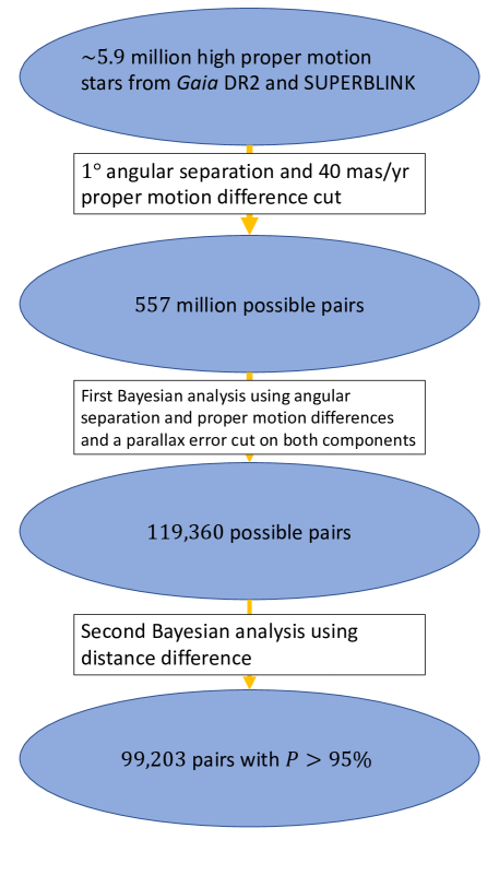
Figure 1: Flow chart demonstrating the method used to construct the SUPERWIDE catalog. Starting with a sample of $\sim 5.9$ million high proper motion stars, we conduct a two-step Bayesian analysis to determine which stars are part of wide binaries. This analysis takes into account angular separations, proper motion differences and distance differences.

The color-magnitude diagrams for these high probability pairs are presented in Figure 2. Primary stars are shown in the top panel while secondaries are shown on the bottom panel, with “primary” and “secondary” being determined by brighter $G$ magnitude. For both panels, the main sequence is well defined and in the color range of the K-dwarfs, $G_{BP}-G_{RP}$ from 1.01 to 1.81, a doubling of the main sequence can be distinguished as a secondary sequence of objects vertically shifted up by $\sim 0.7$ magnitudes, looking much like a “halo” above the standard main sequence. This doubling is believed to be caused by the presence of unresolved companions. While young stars can cause a similar effect as they fall onto the main sequence, as they have yet to fully contract and remain overluminous due to their larger sizes compared to normal main sequence stars, we note that the SUPERWIDE catalog was constructed from a high proper motion sample which is biased against young, field stars, which typically have low relative motions to the Sun and thus are under-represented in high proper motion subsets.

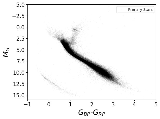
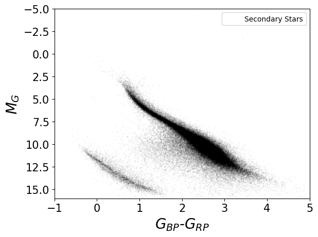
Figure 2: Color-magnitude diagrams for the 99,203 pairs with Bayesian probabilities $>95\%$ of being wide physical binaries. Top: Color-magnitude diagram for the primary components. Bottom: Color-magnitude diagram for the secondary components. Primary stars are found of all types, including notable subsets of red giants, subgiants, more massive main-sequence stars, and white dwarfs. Secondaries are overwhelmingly low-mass stars and white dwarfs. One notable feature is the vertical “thickening” of the main sequence for low-mass M stars (Gaia $G_{BP}-G_{RP}$ $>2$).

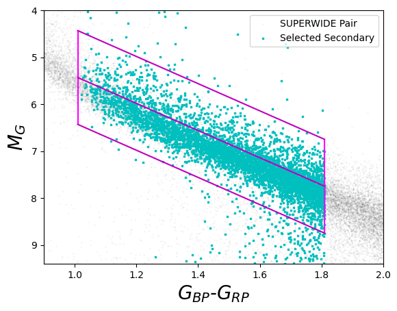
Figure 3: H-R Diagram for SUPERWIDE with the K+K wide binary selection shown. The magenta box defines the K dwarf main sequence plus overluminous stars. The line going through the middle represents the arbitrary reference line $[M_{G}]_{Kref}$ that is used to define the overluminosity factor for each wide binary. Red points show the primary stars and the cyan points show the secondary stars selected for our light curve search.

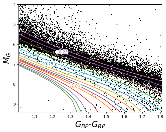
Figure 4: Color-magnitude plot for MIST isochrones in the K dwarf region. Black points are the components of K+K wide binaries from our sample. Different color lines represent different metallicity tracks. The three labels shown show the metallicity for the same colored lines. Going from the +0.50 line to the -2.00 line, each different line represents a decrease of 0.25 in metallicity. This increase to 0.5 after the -2.00 line.

To examine this doubling, Hartman & Lépine (2020) focused on the K-dwarf regime and took a sample of 2227 K+K wide binaries with primary distances less than 250 pc and Bayesian probabilities $>99\%$ along with a cut based on color and absolute magnitude. Additionally, they revised their definition of “primary” and “secondary” to be defined by $G_{BP}-G_{RP}$ color rather than Gaia $G$ magnitude, with the component with a bluer color assigned as the primary star. In this paper, we expand upon the previous analysis in Hartman & Lépine (2020) by defining an expanded sample of K+K wide binaries from the 99,203 high probability wide binaries from the SUPERWIDE catalog. In a similar manner to Hartman & Lépine (2020), we focus on stars withing a set color range $1.01<G_{BP}-G_{RP}<1.81$ as seen by the magenta boxes in Figure 3. Like Hartman & Lépine (2020), our primary and secondary designations were initially determined by Gaia $G$ magnitude, but are now changed to $G_{BP}-G_{RP}$ color; thus, we require each component to have both a $G_{BP}$ and $G_{RP}$ magnitude. Unlike our previous work, we do not set a limit on absolute magnitude dependent on color. We put limits so that the primary absolute magnitude is fainter than $M_{G}=4$ and the secondary magnitude is brighter than $M_{G}=9.4$; this eliminates red giants and white dwarfs from the subset. In addition, we no longer restrict our sample based on distance, which greatly expands our selection. We also lower our probability limit to 95% as the majority of pairs in the 95%$<P<$99% are still real binaries. The rationale for this shift is to include more binaries that are likely to be genuine wide binaries to increase the size of the sample for improved statistics. This revised selection doubles the sample to 4947 candidate K+K wide pairs. The color-magnitude diagrams for our selected binaries (with primaries in top panel and secondaries in bottom panel) are shown in Figure 3. The magenta box represents our area of focus for this analysis and will be discussed below.

A complicating factor in this analysis is the effect of metallicity difference between stars of similar mass, commonly known as “cosmic scatter.” To show how metallicity trends in the K-dwarf regime, we use the MIST isochrones (Paxton et al., 2011, 2013, 2015; Dotter, 2016; Choi et al., 2016; Paxton et al., 2018) to model the metallicity tracks for solar age stars, with metallicity being $[Fe/H]=\log((Fe/H)_{star}/(Fe/H)_{sun})$. This is shown in Figure 4. We used the isochrones matching an age of $10^{9.65}$ years, $\frac{v}{v_{crit}}=0.4$ and Gaia magnitudes. Starting from +0.5 in metallicity, these isochrones go to -4.0 in steps of 0.25 between +0.5 to -2.0 and then in steps of 0.5 between -2.0 and -4.0. For most metallicity tracks down to -1.0, the metallicity tracks run parallel to each other in the K-dwarf regime. In addition, we provide the distribution of projected physical separations as a function of distance and the histogram of projected physical separations for this sample in Figure 5, showing that our binaries span a wide range of distances and physical separations. The two red lines represent the effects of the angular separation cuts applied in Hartman & Lépine (2020) at $2\arcsec$ and $3600\arcsec$, respectively.

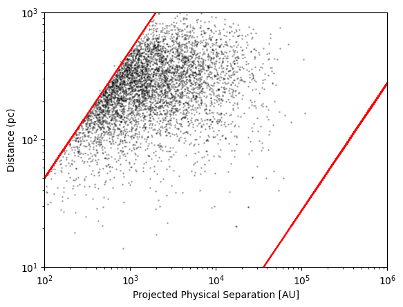
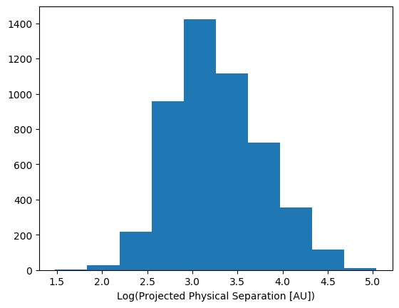
Figure 5: Top panel: Projected physical separation as a function of primary distance for the selected sample. Most pairs reside between 100-600 pc. Red lines indicate the 2″and 3600″cuts that are part of the SUPERWIDE catalog. Bottom panel: Distribution of projected physical separations for the selected sample.

2.2 Light Curve Retrieval

Starting with this sample of 4947 pairs, we cross-match our all primaries and secondaries with the TESS Input Catalog (TIC) by matching the Gaia DR2 identification numbers in common between our sample and the TIC catalog using the modules astropy and astroquery (Astropy Collaboration et al., 2013, 2018; Ginsburg et al., 2019). Using the associated TIC ids, we use the Lightkurve package available in Python to search for TESS, K2 and Kepler targets and recover their light curves (Lightkurve Collaboration et al., 2018). We retrieve all available sets of data for each target. However, we examine each sector separately. We first check if the target has available two-minute cadence light curves and download both the Simple Aperture Photometry (SAP) and Pre-search Data Conditioning SAP (PDCSAP) light curves. If a target does not have two-minute data, we then check for data products from the MIT Quick Look-up Pipeline (QLP, Huang et al., 2020a, b) and retrieve both the available light curves that resulted from their light curve extraction algorithm (SAP) and then light curves which underwent post-processing to remove stellar activity and instrumental noise which are referred to as KSPSAP . If a star does not have either of those, we search for any K2 light curves and then finally for Kepler light curves.

We find 2928 primaries and 2494 secondaries that have light curves available from at least one of the missions. Of those, 2463 are from the same binary system, i.e. we find 2463 pairs where a light curve is found for both the primary AND secondary component. To be clear, each component has its own TIC number, however, in many of the cases, the light curves are essentially the same due to their proximity on the sky and the large size of the TESS camera pixels. Our analysis finds that, of the 2463 pairs with both components having a light curve, 2047 have angular separations less than one TESS pixel (21″) while only 168 have angular separations larger than two TESS pixels (46″). Therefore, the majority of the light curves for these systems blend the light from both stars unless a K2 or Kepler light curve is retrieved. While this generally prevents us from knowing for sure from which of the components (primary or secondary) any signal is coming from, it still allows us to effectively search for eclipsing or rotating systems in both components at the same time. Further ground-based photometric validation will however be needed to confirm which component is responsible for any modulation of the signal.

In some cases, the signal may also be from a third star in close proximity to the pair. However, we believe this to occur in a low number of our systems. To examine this, we searched around each star in our sample for third stars within Gaia DR2 that might contaminate the light curve. We required that any other star near the searched star must not be its wide binary companion, have a Gaia $G$ magnitude brighter than 18, and have a $\Delta G$ magnitude difference of less than 4. We searched for stars within one TESS pixel (21″) and within two TESS pixels (42″). We found that around 2% had another star within one TESS pixel that could interfere with the signal from the target star and around 10% had another star within two TESS pixels. Due to the low probability of contamination indicated by these results, we will assume that if a periodic signal is detected in our analysis, it is from the target system and not a nearby field star. This does not rule out the need for follow-up observations to confirm where the modulations are coming from for the reasons stated in the previous paragraphs.

2.3 Periodogram Analysis

In order to identify systems with significant photometric modulations, we examine each of the light curves visually and sort them into one of four possible bins based on morphology: (1.) eclipsing/transiting system, (2.)fast rotators with periods less than five days, (3.) slow rotators with periods greater than five days and (4.)systems that show both rotation and eclipses; one example from each of these groups is seen in Figure 6. Eclipsing systems are easily identified from the dips in the light curves caused by another object passing in front of the target star while modulations from a fast/slow rotator show a sinusoidal/variable pattern which is due to spots on the surface of the star coming in and out of view.

We then conduct a periodogram analysis on these systems using the periodogram function from the Lightkurve package. For the eclipsing systems and those systems that show both rotation and eclipses, we run this analysis twice using the Lomb-Scargle (Scargle, 1982) and Box-Least-Squares (BLS) (Kovács et al., 2002) methods to identify and measure a period for the eclipses. In most cases where the light curve is produced by the QLP, we use the KSPSAP fluxes. This allows due to the removal of long term stellar trends for an easier calculation of the eclipsing binary’s period. Additionally, the rotation in these systems is found to be overwhelmingly in sync with the eclipses, for a good reason as tidal forces in close binaries will usually synchronize the rotation of both stars with their orbital period. However, the light curves for several stars showed more noise in the KSPSAP flux than the SAP flux and, in these cases, we used the SAP flux to generate the light curves and the resulting phased light curves. For the TESS two-minute, K2, and Kepler data, we use the PDCSAP fluxes to calculate the binary’s period to take advantage of the cleaner data that the PDCSAP fluxes offer compared to the SAP fluxes.

After this first examination, the period is fine-tuned by hand to create a clean, phased light curve for each eclipsing/transiting system. We conduct this analysis on the primary stars first and, if a secondary light curve for the same binary is found, we use the period of the primary to construct the phased light curves for the secondary if the same type of signal is seen. We do note that no additional modeling has gone into this analysis as just identifying these systems as eclipsing/rotators suits the purpose of this study.

We run this analysis again on the systems that are identified as showing rotation. In this case, we only use the Lomb-Scargle method as it can pick out the rotation signal better than the BLS method and we use only the SAP light curves unless the light curve is from K2 or Kepler, in which case we use the PDCSAP light curves. This choice was made to avoid any potential cases where the detrending that is applied to the PDCSAP and KSPSAP from the QLP light curves could affect the stellar activity signals we hope to detect. Additionally, we restrict the periods examined depending on whether the star was visually determined to have a rotation period greater than or less than five days from the visual analysis. We again stress that just being identified as a fast or slow rotator suits the purpose of this study. We leave it to a future paper to fully model the rotation signals in our identified rotators. Much like the eclipsing/transiting analysis, if a secondary light curve is found with a primary counterpart, we use the primary’s period to construct the phased diagram and see if this produces an acceptable phased light curve. In any case, the identification of an accurate rotation period for a starspot signal is always elusive, as differential rotation in main sequence stars means that spots will move in and out of view at slightly different rates depending on their latitudes, and the period of the modulation will vary over time as the spot pattern changes. Additionally, we find several systems where multiple variable signals are shown. For these, we note both periods in our results but only count the system towards our analysis once.

3 Results

In total, our search recovers 42 eclipsing/transiting systems, 16 systems showing both rotation and eclipses/transits, 105 systems showing rotation with a period less than 5 days, and 101 systems showing rotation with a period slower than 5 days. We split these results into two groups. In Tables 1, 2, 3, and 4, we present the results for binaries which are two stars in the eyes of Gaia. In Tables 5, 6, 7, and 8, we highlight the systems that are higher-order multiples in the eyes of Gaia already. These systems are discussed further in Section 3.3. In each of these 8 tables, the columns are Gaia DR2 ID Numbers, R.A. from Gaia DR2, Decl. from Gaia DR2, Gaia $G$ magnitude, Gaia $G$ flux error, NASA mission (either T-2min for TESS 2 minute light curve data, T-QLP for TESS data products from the QLP, K2 or Kepler), and mission ID (either TIC or Kepler catalog) for both components. This is followed by the determined periods for components 1 and 2 with the final column being the SUPERWIDE angular separation. Component 1 is the primary star as determined by bluer $G_{BP}-G_{RP}$ color and component 2 is the secondary for the true wide binary tables (1 - 4). This assignment method is kept for the resolved triples; however, the other components are not taken into account.

In many of these cases, the light curves are the same for the two components except with slightly different base flux levels, which means that the TESS camera did not fully resolve the two components, and the measured light curve is that of the blended primary and secondary flux. This means that although both components’ light curves may show a variable signal, one of the components may not be variable. Figure 6 shows examples of the original and phased light curves for stars from each of the four bins that we defined. Within the tables, $P_{1}$, period of component 1 (primary), and $P_{2}$, period of component 2 (secondary), are determined in this manner. If only one component has a variable signal detected in the light curve analysis, then that component is assigned the determined period from the light curve analysis. If both components show variability and the period is different between the two, then both periods are reported. Finally, if both components show variability and the period is the same, then the Gaia flux error for each component is used to guess which component most likely houses the binary or stellar rotation signal with the component with the higher Gaia flux error assumed to be the variable object. Follow-up observations will be needed to confirm that our guess made here is correct.

In a separate table, we highlight two wide binary systems where both components show signs of multiple sources of stellar modulation. This is shown in Table 9. The two systems in question have evidence of either two or three stellar modulation signals in their periodograms. We present the resulting periods in three columns of Table 9 with the rest of the columns being the same as in Tables 1 - 8.

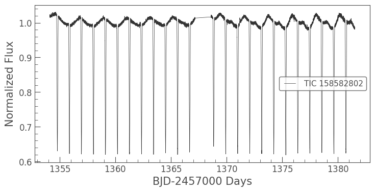
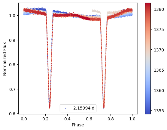
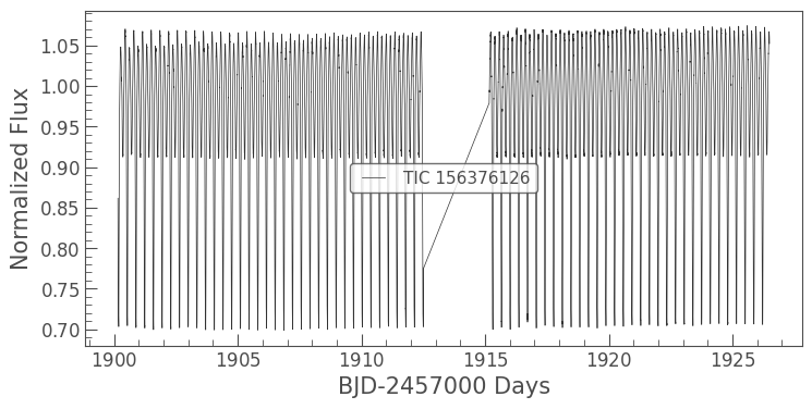
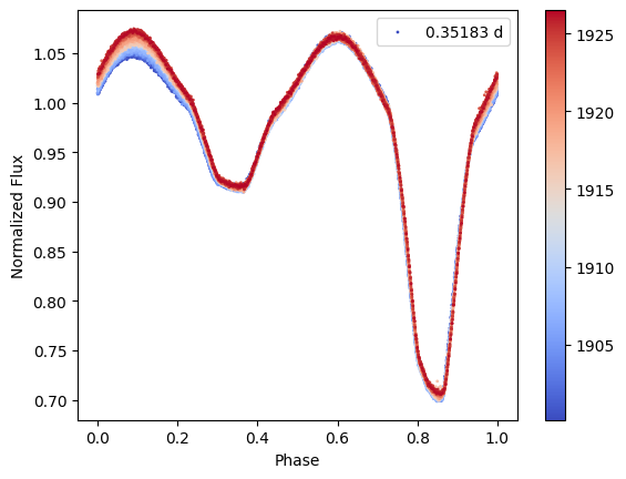
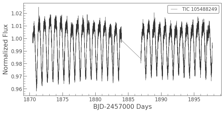
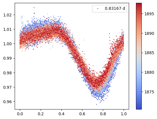
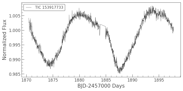
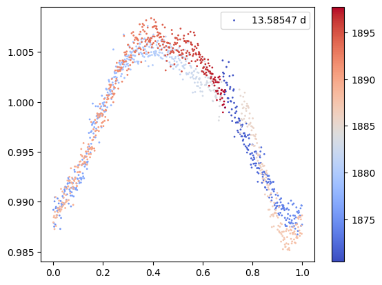
Figure 6: Examples of light curves and phased light curves for four primary stars in our sample. Each plot pair shows the light curve obtained through Lightkurve on the left and the phased light curve on the right. The period used for the phase folding is shown in the right panel for each star with the identifier for each star shown in the light curve plot. Phased light curve points are colored by their time in the unphased light curve. Top: Example of a system with both rotation and eclipses, Top-middle: Example of eclipsing system, Bottom-middle: Example of a system with rotation less than 5 days, and Bottom: Example of a system with rotation more than five days. The different colored points and the color bar for the phased light curves show the epoch of the data points.

3.1 Testing the Lobster Diagram

As a test of the overluminosity correlation between primaries and secondaries in K+K wide binaries, we decided to re-examine the so-called “Lobster diagram” (Figure 7) and assess where systems with eclipsing/rotator signals fall on the diagram. Hartman & Lépine (2020) defined the “overluminosity factor” ($F_{OL}$) as,

$$F_{OL}=M_{G}-[M_{G}]_{Kref}$$

where $[M_{G}]_{Kref}$ is a reference value representing the absolute magnitude of a single-star K-dwarf of the same color with a set reference metal-abundance. We adopt the same definition of the overluminosity factor, ($F_{OL}$), with one key exception: in Hartman & Lépine (2020), the $M_{G}$ for each component was used separately in the calculation of $F_{OL}$. However, we make a smaller but significant modification for this paper. Since these are high probability wide binaries, their parallaxes should be nearly identical in most cases, as the orbital separations are much less than 1 pc. It is thus fair to assume both stars are at the same distance, rather than introduce uncertainties from parallax measurement errors. As such, for each binary, we adopt for both stars the parallax of the component that has the smallest parallax error in the Gaia DR2 catalog. We keep the same definition of $[M_{G}]_{Kref}$ as:

$$[M_{G}]_{Kref}=2.9(G_{BP}-G_{RP})+2.5$$

This relationship is represented by the middle magenta line in both panels of Figure 3. The line roughly tracks the division between the single star main sequence and the unresolved binary locus, although this choice is arbitrary. A positive $F_{OL}$ means the component falls below the middle magenta line in Figure 3, while negative $F_{OL}$ means the component is above the line.

The “Lobster diagram” exploits the fact that stars in wide binaries are expected to form within the same star-forming region and should fall on the same metallicity tracks on the H-R diagram. In most cases, these tracks are expected to run parallel to the fiducial line we have defined. In the “Lobster diagram,” the $F_{OL}$ values of the secondaries are plotted against the $F_{OL}$ of their associated primaries, with each pair represented by a single point. Pairs with no unresolved companions should fall on a 1:1 locus because their $F_{OL}$ values will be similar. On the other hand, the presence of an unresolved companion will increase the flux from one of the components (primary or secondary), and shift the point for that pair off the track, effectively revealing that the two components have values of $F_{OL}$ that do not agree with one another. The magnitude of this shift will depend on the flux ratio between the star and its unresolved companion, which is related to the binary mass ratio, q, for main sequence stars.

For this part of the analysis, we first remove any resolved higher-order multiples (to be discussed in a later section.) This sets aside 300 pairs from our initial sample of 4947. We show the overluminosity plot for most of the remaining 4647 wide binaries in Figure 7, with 4268 systems falling within the shaded regions shown. Several hundred pairs are not seen in this plot as one of the component’s overluminosities falls outside of the plot limits. The limits of the plot happen to correspond to the area bound by the magenta box in Figure 3 and, for a point to appear in Figure 7, both components must fall in the Figure 3 magenta box. This is examined more in Section 3.4.

There are four distinct regions in Figure 7. The area defined by the solid red lines, the body of the “Lobster”, represents where pairs with two “single” components reside as their overluminosity factors are roughly the same. This region is defined as the following:

$$-0.1<F_{OL,pri\&sec}<1.0$$

$$F_{OL,pri}>F_{OL,sec}-0.13$$

$$F_{OL,pri}<F_{OL,sec}+0.13$$

This forms a “true wide binary” sequence composed of two single stars. This was visually determined to match the observed density of points in this area with pairs with $F_{OL}>1.0$ and $F_{OL}<-1.0$ being considered suspicious (to be discussed later). The two yellow shaded areas represent the areas where one component is unusually overluminous compared with its companion, as expected if it is an unresolved binary system, indicating the system is actually a triple. Which way the pair deviates from the body of the “Lobster” determines which component is the possible unresolved binary. If the primary is overluminous, then the pair will fall below the “true binary” (1:1) sequence whereas if the secondary is overluminous, then the pair will fall to the left of the sequence. In both cases, the yellow areas extend away from the 1:1 line by 1 magnitude both below the line and to the left of the line for $F_{OL,pri/sec}>0.0$. For $-0.1<F_{OL,pri/sec}<0$, only the area between $-1<F_{OL,pri/sec}<-0.1$ is considered as there was concern of sub-giant and giant contamination for pairs. The purple shaded area represents the area where both components are unusually overluminous making the wide binary a possible quadruple system and is simply defined as a box with $-1<F_{OL,pri/sec}<-0.1$. The regions denoted by the dashed red lines, the “claws” of the lobster, represent the area where unresolved systems with equal mass ($q\sim 1$) are expected to cluster: these two regions are offset from the body by about 0.7 mag in overluminosity factor, which matches what is expected for an equal mass unresolved system on the color-magnitude diagram. In fact, the “claws” do show a definite over-density of objects, which is evidence for just such a sequence of unresolved, equal-mass close binaries. Currently, the “Lobster diagram” only works well for wide binaries in the K-dwarf range, as the slope of the main sequence follows a linear color-magnitude relationship, sequences for stars of different metallicities have the same slope and the metallicity spread of the stars is relatively small, which is not the case for stars in the M-dwarf range, for example, where the color-magnitude-metallicity relationship is more complex.

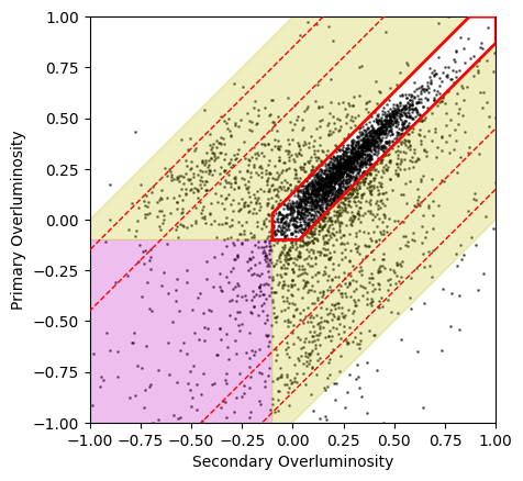
Figure 7: The “Lobster diagram” plotting the overluminosity factor $F_{OL}$ of the primary star as a function of the $F_{OL}$ of the secondary star for the most of the 4647 K+K wide systems in the assembled sample. Two key features stand out in this plot. The dense locus along the 1:1 line represents “true” wide binaries where both components are single in the eyes of Gaia. Points lying outside of this locus represent systems where unresolved components make either the primary or secondary components suspiciously overluminous. If a point falls in the purple region, it may represent a possible quadruple system or a young system, where both components are unusually overluminous.

Using the binaries in Figure 7 to define the baseline, we plot out the locations of the eclipsing systems, systems showing rotation periods larger than 5 days (slow rotators), systems showing rotation periods less than 5 days (fast rotators), and systems showing both rotation and eclipses. These are shown in the different panels in Figure 8. 22 pairs were not included on this plot, 5 eclipsing systems, 8 fast rotators, and 7 slow rotators. For most of these systems, the reason for their exclusion was because one component’s overluminosity was outside of the range of the plot and outside the magenta box in Figure 3. As discussed further on, we only examine pairs which fall within the shaded regions of Figure 8 for this analysis.

Examining the four panels in Figure 8, we can verify if the “Lobster diagram” works as a possible method to determine if individual components of K+K wide binary systems are unresolved binary systems themselves. In the plots of eclipsing systems and systems that show both rotation and eclipses (top panels, Figure 8), we do confirm that the vast majority of systems with light curves classified in either of these two groups fall outside of the true wide binary sequence. For the eclipsing systems, $78.9\%\pm 20.7\%$ lie in the shaded regions of the top left panel of Figure 8, while $84.6\%\pm 34.7\%$ lie in the shaded regions in the top right panel for the systems that show both rotation and eclipses with errors calculated using Poisson statistics. We do not include systems that fall completely outside of the shaded regions or the true wide binary sequence. For eclipsing systems that fall within the true wide binary sequence, there are two possible explanations. First, the flux ratio between the companion that is eclipsing and the target star is small. In this case, Gaia would not pick up the excess flux from the faint component and the magnitude would be consistent with that of a single star. Second, the light curve may be picking up eclipses from an unrelated background star caught in the TESS camera. As mentioned previously, TESS pixels are large and can register the light from multiple stars in a single light curve; further follow-up would be needed to confirm this idea. We also note that for those systems where only one component has a light curve that shows eclipses, the “Lobster diagram” correctly identifies whether the primary or secondary hosts the companion. With these caveats, we believe that we have demonstrated that the “Lobster diagram” method is an efficient tool for identifying probable close companions in these wide binaries.

Examining the light curves further, we examine the fraction of rotating stars that lie outside of the true wide binary sequence. For the stars with rotation periods less than five days (lower left panel, Figure 8), $73.5\%\pm 12.4\%$ lie in the shaded regions. This significant result suggests a link between overluminosity and fast rotation, with the most likely explanation being that the fast rotation is caused by tidal synchronization of the rotation and orbital period in the close binary systems. The fact that no eclipse is recorded simply indicates that the inclination of the system does not allow us to see the eclipses. On the other hand, for stars with rotation periods greater than five days (lower right panel, Figure 8), only $42.0\%\pm 8.6\%$ lie in the shaded regions, potentially pointing to their rotation and overluminosity not being related.

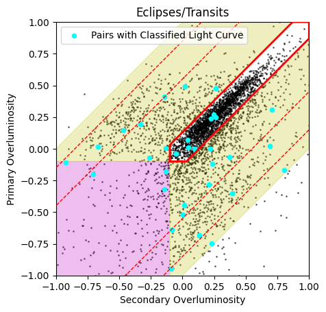
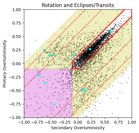
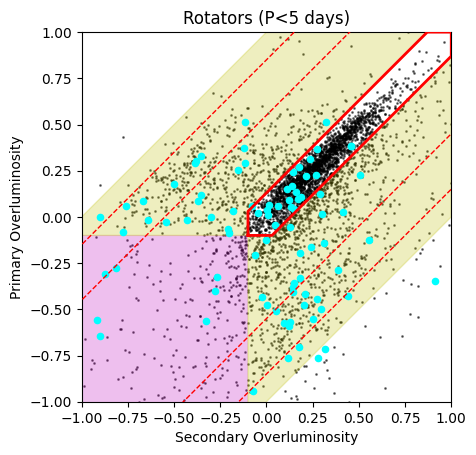
Figure 8: Overluminosity plots highlighting the locations of TESS light curve targets (aqua points) that have been sorted into one of our four bins going from upper left to bottom right: (1.) systems where one component shows eclipses/transits, (2.) systems where one component shows both rotation and eclipses, (3.) systems where one component is a fast rotator ($P<5$ days), and (4.) systems where one component is a slow rotator ($P>5$ days). Note that for the systems where a component shows either an eclipse or transit or is a fast rotator, most show at least one component to be overluminous, whereas slowly rotating systems are mainly in the “true” wide binary sequence.

3.2 Additional Evidence from Gaia and the Multiple Star Catalog

To provide additional evidence that the “Lobster diagram” finds unresolved companions, we can examine the Gaia data itself. The Reduced Unit Weight Error (RUWE) parameter is an indicator of how good the astrometric fit is for a given star and can be used as a powerful tool to identify unresolved binaries within Gaia (Belokurov et al., 2020; Stassun & Torres, 2021; Penoyre et al., 2022). Single stars with good astrometric fits typically have a RUWE between 1.0 and 1.4, although Stassun & Torres (2021) found evidence in a sample of eclipsing binaries systems that an eDR3 RUWE value in that range does not guarantee that a star does not have an unresolved companion. As a test of the “Lobster diagram,” we recover the Gaia DR2 RUWE values for our sample and, for each pair, we take the larger RUWE value from either component as the value for the system. We then select the pairs with RUWE$\geq 1.4$ as systems potentially hosting unresolved companions and plot them on the “Lobster Diagram” in Figure 9. Using the same method as in the previous section, $77.5\%\pm 3.9\%$ of these systems reside outside of the true wide binary sequence agreeing with our findings from the light curve analysis.

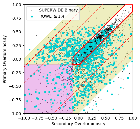
Figure 9: “Lobster Diagram” with pairs where one component’s RUWE value from Gaia DR2 is $\geq 1.4$ shown by the highlighted points. The overwhelming majority of points lie outside of the true wide binary sequence (region bordered by solid red line).

Finally, we cross-match our sample of 4647 systems with the Updated Multiple Star Catalog available on Vizier (Tokovinin, 2018). This catalog mostly consists of systems that are known to have 3 or more members. We find 20 systems that are matches to the Multiple Star Catalog, all of them known to be triples with an unresolved third component. Putting these 20 systems on the “Lobster” diagram in Figure 10 and applying the same criterion for the parallax used the calculation of the overluminosity for each component, we see that half of the systems fall on the true wide binary sequence, but the other half fall in the region where unresolved binaries are expected to reside. Based on the data provided by the Multiple Star Catalog, the systems that fall in the unresolved binary regions mainly contain a component that is a double-lined spectroscopic binary while the ones that reside in the true wide binary sequence either contain a component that is a single-lined spectroscopic binary or a binary that is resolved with high angular resolution imaging. As we are using the overluminosity of a component to tell if it has an unresolved companion, it follows that if the unresolved companion is faint, it will not contribute light to the system and will appear as a single star.

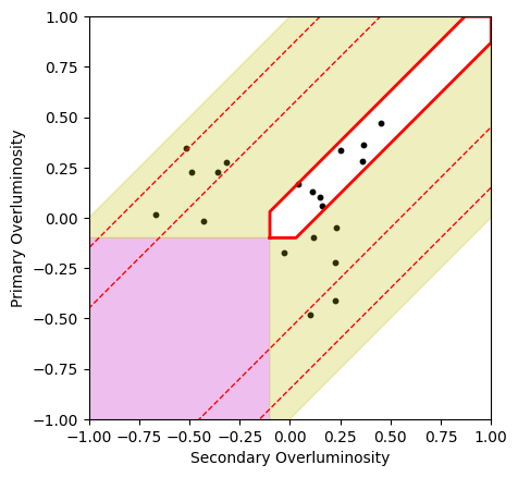
Figure 10: Overluminosity plot for systems that are in SUPERWIDE as only two stars but are listed in the Multiple Star Catalog (Tokovinin, 2018) as having a known unresolved companion. Systems outside the body have a bright unresolved companion that is detected as either a double-lined spectroscopic binary or a companion detected by speckle imaging. Systems in the body are either faint companions detected by speckle imaging or single-lined spectroscopic binaries.

3.3 Resolved Higher-Order Multiples

In the section above, we deliberately excluded 300 “pairs” that we identified as being part of resolved higher-order multiple systems in Gaia DR2; these are common proper motion systems of 3 or more resolved stars; each of these systems may contribute multiple "pairs" (since triples make 3 pairings, quadruples 6 pairings, etc.). We now come back and address these systems as a group. For our light curve analysis, we simply searched all 300 “pairs” for available TESS, K2 or Kepler light curves. Among our detections, we find 4 systems with eclipsing binaries, 14 systems with a component showing rotation faster than five days, 13 systems with a component showing rotation slower than five days and 4 systems showing both rotation and eclipses/transits. We plot the location of these pairs on the overluminosity plot in Figure 11 using the same method as in Figure 8. We only plot the K+K pairings of the resolved higher order multiples as that is what works on the lobster diagram, though some systems consist of all K-dwarfs (and contribute multiple “pairs”), while others are K+K+something else (and contribute just one “pair” on the plot). One of the systems showing both rotation and eclipses/transits falls outside of the window shown in Figure 11. The same trends are observed showing that the majority of fast rotators and eclipsing systems fall outside of the true wide binary sequence while systems with slower rotation rates are more likely to be fall in the true wide binary sequence.

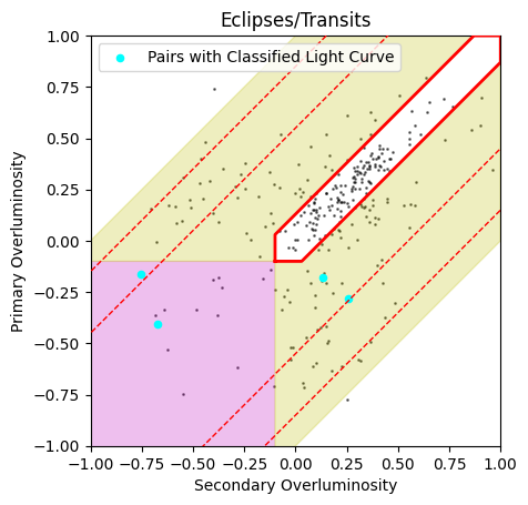
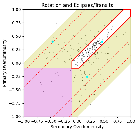
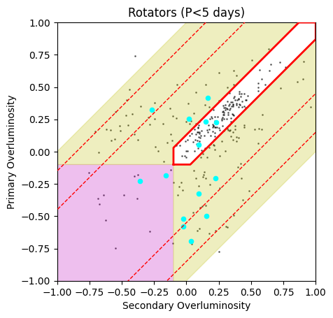
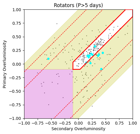
Figure 11: Overluminosity plots highlighting the locations of TESS light curve targets for resolved higher-order multiples from Gaia DR2. Same format as in Figure 8. Some systems with TESS light curves fall outside of the range for this plot.

In Figure 11, we include all 300 “pairs” in the overluminosity plots. However, for the next sections dealing with the higher-order multiplicity of K+K wide binaries, we only include a small number of higher-order multiples in our analysis. The main reason for this is we want to only include resolved higher-order systems in those cases where if the system had been a wide binary with an unresolved companion, it would have made it into our sample. This means we only include resolved systems consisting of a wide K+K pair and then a resolved closer K+something else system, where that something else is a K-dwarf or lower mass (M-dwarf). Due to the way the SUPERWIDE catalog handles higher-order multiples, each possible pairing in a multiple system has its own entry in SUPERWIDE, i.e. a resolved triple will have 3 entries in SUPERWIDE, one for each pairing of components. However, there are resolved higher-order systems in SUPERWIDE where there are only two entries; this is due to the $2\arcsec$ limit in SUPERWIDE so the two entries match to the “pairs” between the closer binary and the wide companion. For these systems, we calculate the separation between the close binary in the system. Taking these 300 “pairs,” we require each system to pass several cuts to be included in our analysis. The projected physical separation of the K+K pair in the resolved system must not have the smallest separation of the “pairs” in the resolved triple, each “pair” in the resolved triple has a probability $>95\%$, and all other stars in the system must be K-dwarfs or lower mass. These cuts result in a sample of 45 resolved higher-order multiples.

3.4 Estimating the Higher-Order Multiplicity of K+K Wide Binaries

One of the key features of the overluminosity plot is that it can be used to put a lower limit on the higher-order multiplicity of the K+K wide binaries based on the assumption that all pairs outside of the “true” wide binary sequence contain unresolved companions. This will be a lower limit because not all stars with unresolved companions will appear as overluminous, as hinted from the light curve analysis which strongly suggests that unresolved systems with large mass ratios will not register as being overluminous. To estimate the higher-order multiplicity fraction, we use the sample of 4647 binaries where the higher-order multiples have been excluded as they are already higher-order multiples.

While in Hartman & Lépine (2020) we counted everything that was not in the true wide binary sequence, this time we only count binaries as overluminous if they lie in the shaded regions of Figure 7, i.e. we exclude objects that have such large overluminosity values in one component that they are considered suspicious, and assumed to be contaminants ($F_{OL,pri/sec}>1.0$ and $F_{OL,pri/sec}<-1.0$). There are two populations that are most impacted by this. Pairs containing sub-giant and giant stars are removed from the sample; They are assumed to be the points in Figure 7 that lie outside of the shaded regions in the lower right and pairs that are above the magenta box in Figure 3. Metal-poor pairs with metallicities less than around -1.0 are also removed; they are assumed to be the points below the magenta box in Figure 3. Both populations have large overluminosity values for two different reasons. The sub-giants and giants appear overluminous as they are evolving off the main sequence with one component far above the main sequence and can be confused as unresolved binaries in our analysis. The metal-poor stars appear overluminous because our assumption that the metallicity tracks are parallel to the straight line we defined as our reference breaks down for lower-mass, metal-poor systems. This can be seen by comparing the -2.00 and +0.25 lines in Figure 4 across the entire K-dwarf region. While they may be initially parallel from $1.0<G_{BP}-G_{RP}<1.1$, the slopes of the two lines rapidly diverge at larger $G_{BP}-G_{RP}$. As our reference line for the calculation of $F_{OL}$ is roughly parallel to the metal-rich and solar metallicity tracks, this divergence breaks the correlation between the components of metal-poor stars and causes one or both of the components to have $F_{OL}>1$. To avoid this issue, we remove 379 pairs which fall outside of the shaded regions in the “Lobster Diagram.”

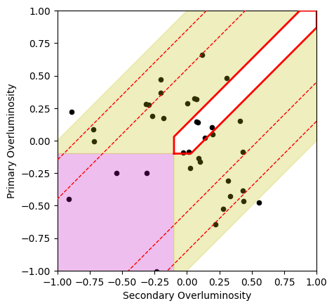
Figure 12: Overluminosity plot for systems that are resolved higher-order multiples in SUPERWIDE, consist of a wide K+K pair, and do not include higher mass members. For the calculation of the higher-order multiplicity, we only count systems which fall in the body of the “Lobster Diagram” or in the shaded regions.

With the remaining 4268 systems, we find that 259 fall in the purple shaded region representing possible quadruple systems, 1056 and 627 respectively fall in the yellow shaded regions below (primary component overluminous) and to the left (secondary component overluminous) of the true wide binary sequence, while the remaining 2326 systems fall in the true wide binary sequence. Additionally, we include the resolved higher-order multiples that were removed from the analysis previously. We take the sample of 45 higher-order multiples that were identified in Section 3.3 and combine the pairs with the shortest separations. This creates a sample of “binaries” where one or both components are treated as an unresolved system. Most of the higher-order multiples are triple systems with 2 quadruple systems in a 2+2 configuration where both close binaries are K+M pairs. We apply our analysis to these systems and show the resulting “Lobster Diagram” in Figure 12. We find that 3 systems are possible quadruple systems, 27 show signs of having an unresolved binary as one component and 7 fall on the true wide binary sequence. Therefore, we count 30 of the higher-order multiples as overluminous and count 37 towards the total number. 8 systems fall outside of the shaded regions and are not included in the analysis.

Taking those systems of the 4268 that were not resolved higher-order multiples that fall outside of the true wide binary sequence plus the higher-order multiples discussed in the previous paragraph, we calculate a lower limit on the higher-order multiplicity fraction of $45.8\%\pm 1.2\%$, with the error calculated with Poisson statistics. This is roughly six percentage points higher than our $39.6\%\pm 1.6\%$ estimate from Hartman & Lépine (2020). We suspect this may be due to contamination from evolving (sub-giant) stars in the early K-dwarfs, $1.01<G_{BP}-G_{RP}<1.2$, which have been added after the removal of the distance limit used in Hartman & Lépine (2020), despite our best attempt at minimizing their presence (see above). In Figure 3, there appears to be a steady increase in the density of points above the middle magenta line as one goes from $G_{BP}-G_{RP}$ of 1.2 to $G_{BP}-G_{RP}$ of 1. This increase moves steadily further away from the magenta line as one goes to lower $G_{BP}-G_{RP}$ color. This sub-population is also evident in Figure 7 as a concentration of stars located directly below the true wide binary sequence. We believe that the majority of these binaries have a primary component that is beginning to evolve off the main sequence and is thus overluminous simply because of old age. Figure 13 shows the “Lobster Diagram” for the sample excluding binaries with $G_{BP}-G_{RP}<1.2$. Using this smaller subset of 2251 binaries and including the 19 resolved higher-order multiples that satisfy this revised color cut (16 of which fall in the shaded regions), we determine a higher-order multiplicity fraction of $40.0\%\pm 1.6\%$, roughly equivalent to our previous result.

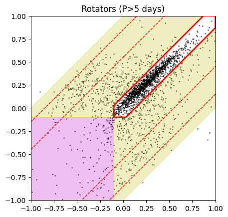
Figure 13: Overluminosity plot for K+K wide binaries with $G_{BP}-G_{RP}>1.2$. Note that the over-density of binaries directly below the true wide binary sequence that was present in Figure 7 is now absent.

3.5 Higher-Order Multiplicity as a Function of Projected Physical Separation

In Hartman & Lépine (2020), we compared the higher-order multiplicity fraction for the whole sample to a selection of extremely wide binaries with projected physical separations larger than 10,000 au. We found that the fractions were similar to within the measurement errors. For this paper, we expand this analysis to a wider range of physical separations. Using the same criteria as was used to calculate the higher-order multiplicity fraction above and including the color cut to remove possible evolving star contamination, we split our sample into 6 bins with the first bin corresponding to all pairs with projected separations less than Log($\rho$)=2.5, going up in steps of 0.5 Log($\rho$) from Log($\rho$) = 2.5 to 4.5, and the final bin spanning all pairs with projected separations greater than Log($\rho$)=4.5. The results are shown in Figure 14 as a function of the average projected physical separation in each bin. This reveals that the higher order multiplicity fraction is uniform at $\sim 40\%$ and does not depend on the orbital separation of the widest component. This is seemingly at odds with our current understanding of the higher-order multiplicity fraction as a function of projected physical separation, from which we would expect the higher-order multiplicity fraction to be increasing with separation, but this is not what we observe.

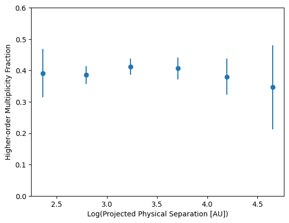
Figure 14: Higher-order multiplicity fraction as a function of projected physical separation for the widest component. Error bars are determined by Poisson statistics. No increase in higher order multiplicity is seen.

3.6 Higher-Order Multiplicity as a Function of Metallicity

One key feature that allows our study to pick out overluminous components in the K-dwarf region is that most of the metallicity tracks are parallel but offset from each other. This enables one to identify possible overluminous components amongst the more metal-poor systems ($M/H\sim-1$), which might otherwise go unnoticed as overluminous metal-poor stars on their own are indistinguishable from more metal-rich stars. Another consequence is that in the “Lobster diagrams,” metal-rich stars are found near the origin at (0,0) while metal-poor stars are shifted to higher $F_{OL}$ values (above and right). To confirm this, we crossmatch our sample of 4647 K+K wide binaries with the catalog of Medan et al. (2021) which provides photometric metallicities for a large sample of K-dwarfs, including most of the primary components in our catalog. These metallicity values are shown color-coded in the “Lobster diagram” in Figure 15. We observe a clear correlation between metallicity and overluminosity ($F_{OL}$) values. Using the photometric metallicity of the primary component as a guide, we split the overluminosity plot into eight equally spaced bins on the “Lobster Diagram,” starting from $F_{OL}=0.0$ and continuing to $F_{OL}=0.8$. This is shown by the blue dashed lines in Figure 15.

We redo our analysis and plot the resulting higher-order multiplicity fraction as a function of the average metallicity of the systems that fall in the true wide binary sequence for each bin in Figure 16. If the primary does not have a photometric metallicity but the secondary does, then we adopt the secondary’s value. To reduce possible contamination from sub-giants as pointed out previously, we require both components to have $G_{BP}-G_{RP}>1.2$. We also include the 19 resolved triples which passed our cuts previously. From Figure 16, we see that the higher-order multiplicity fraction is consistent with having a uniform value over the metallicity range examined with the average value being $37.9\%\pm 1.6\%$. There is a hint of a downward trend with increased metallicity, or perhaps a modest increase in the highest metallicity bin, but it is not clear if these are significant.

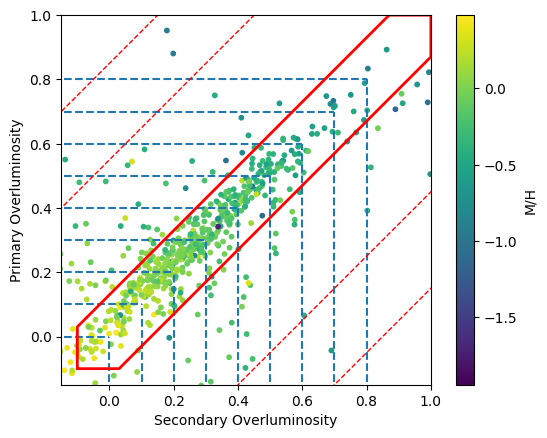
Figure 15: Overluminosity plot for the primary and secondary stars which have photometric metallicities from Medan et al. (2021) and have $G_{BP}-G_{RP}>1.2$ . Color scale represents the metallicity of the stars. Dashed blue lines denote the metallicity bins used for the analysis.

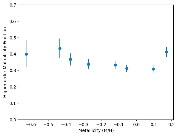
Figure 16: Higher order multiplicity fraction as a function of metallicity. Metallicity values for each point are determined by the average metallicity in the true wide binary sequence of the eight bins shown in Figure 15. Error bars are determined by Poisson statistics.

4 Discussion

4.1 Efficacy of the “Lobster Diagram”

As shown by Figure 8 and Figure 9, the overluminosity plot (the “Lobster diagram”) enables one to identify many close companions that are unresolved in the Gaia DR2 catalog, but can nonetheless be identified as close binaries. The overwhelming majority of components with light curves that show eclipses/transits lie outside the true wide binary sequence, consistent with the expectation that unresolved binaries should be overluminous compared to main sequence stars of the same color. For eclipsing systems that are found to lie along the true wide binary sequence, there are two possible explanations. First, the companion that is eclipsing the target star could be faint, in which case the Gaia photometry would not pick up the flux from the other star and the magnitude would be consistent with that of a single star. Second, the light curve may be picking up the eclipses from an unrelated background star. As mentioned previously, TESS pixels are large and can contain the light from multiple stars in a light curve. Additionally, our RUWE analysis of the “Lobster Diagram” agrees with the light curve analysis in that the majority of systems with high RUWE values, assumed to be unresolved astrometric binaries, do lie outside of the true wide binary sequence. Therefore, when this evidence is combined with the results of our light curve analysis, we conclude that appearing as overluminous on the “Lobster diagram” most likely indicates the presence of an unresolved companion in a wide binary system.

Of further interest is fact that the wide binaries with components that show rotation periods less than five days are also overwhelmingly found outside the true wide binary sequence. This adds more evidence to the belief that fast rotation in older K-dwarfs is likely caused by tidal interactions with an unresolved close binary companion (Angus et al., 2020). Stars spin down with age and high proper motion stars are expected to trend towards older age. Therefore, these systems should be not rotating at periods less than five days, unless there is a close binary companion spinning them up. As SUPERWIDE was created from a sample of high proper motion stars, there should be minimal contamination from young stars which would be the only way to get fact rotation in single stars. As such, we believe these fast rotators are most likely to be binaries in which one component is spun up by the presence of an unresolved companion, which would explain both the fast rotation and overluminosity. This echoes the findings of Simonian et al. (2019) in their examination of fast rotators in the Kepler field which found that 59% of stars with rotation periods less than seven days were overluminous.

4.2 Mass-ratio Limitation of the “Lobster”

While our analysis has shown that the “Lobster Diagram” can identify wide binaries with unresolved close companions, our method depends on Gaia measuring an excess flux in the component with the unresolved companion. This implies there should be a limiting mass ratio, q, below which an unresolved companion cannot be identified with our method. To evaluate this limit, we revisit the MIST isochrones we examined in the beginning of the paper to model where unresolved companions of different q’s and various metallicity values should fall on the overluminosity plot. Figure 4 shows the distribution of MIST isochrones in the K-dwarf region with our sample of K+K wide binaries plotted in the background.

We calculate the overluminosity factors for the primary and secondary components in this manner. For a given solar-age isochrone with a fixed metallicity (a single line in Figure 4), we step through the isochrone over the range of the K-dwarf region we used for this paper, $1.01\leq G_{BP}-G_{RP}\leq 1.81$. At each step, we obtain the mass and Gaia $G$,$BP$ and $RP$ magnitudes provided by the isochrone. We use these to calculate $F_{OL,pri}$ as,

$$F_{OL,pri}=M_{G,double}-[M_{G}]_{Kref}$$

$M_{G,double}$ is the magnitude at the step in the isochrone plus additional light provided by an unresolved companion. The value of the additional light is determined by iterating over all stars in the isochrone with a lower mass, meaning that for each step, we create how $F_{OL,pri}$ varies as a function of mass ratio. $[M_{G}]_{Kref}$ is set as the value of the reference line at the color of the unresolved double. For this part, we define our reference line as a cubic interpolation of the +0.5 metallicity isochrone, top line of Figure 4. For $F_{OL,sec}$, we set the overluminosity to be equal to that of the current step or to be equal to $F_{OL,pri}$ if it was a single star. We do this for each metallicity isochrone seen in Figure 4 and plot the results in Figure 17, with the color scale representing the value of q for each point. Metallicity decreases monotonically along the 1-1 line in Figure 17 going from high metallicity on the left to low metallicity on the right. As we defined our reference line by the +0.5 metallicity isochrone, the sequence originating at (0,0) on Figure 17 represents the q ratio distribution for one step on the +0.5 isochrone as $F_{OL,sec}=0.0$ for all steps on the +0.5 isochrone. From Figure 17, we conclude that we are sensitive to q ratios of roughly 0.5 or higher for most metallicities visible in this region of the overluminosity plot.

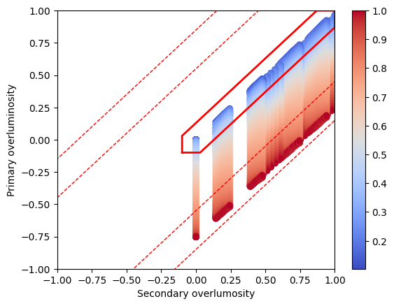
Figure 17: Overluminosity plot using MIST isochrones to examine how mass ratio, q, affects the overluminosity for solar-age isochrones of different metallicities. Color scale represents different q values. We note that unresolved systems with a mass ratio above 0.5 are flagged as overluminous while mass ratios below this value fall within the true wide binary sequence.

4.3 Higher-Order Multiplicity Fraction and Projected Physical Separation

Our results in Figure 14 agree with our previous results from Hartman & Lépine (2020) that the higher-order multiplicity fraction for the whole sample is comparable to that of binaries with projected physical separations larger than 10,000 au. Figure 14 indicates that the higher-order multiplicity fraction is uniform across the range of projected physical separation we are examining. Past studies from Raghavan et al. (2010), Law et al. (2010), Tokovinin (2014a), Tokovinin (2014b) and Moe et al. (2019) have suggested that nearly half of the wide solar-type systems are part of triple systems and have suggested that this value increases with projected physical separation. The difference in the overall multiplicity fraction (our 40.0% vs. $\sim 50\%$ from other studies) can be potentially explained by the fact the we know our study is missing some unresolved companions for several reasons. First, the unresolved companions may be too faint for Gaia to pick up and thus will not show up as overluminous. Second, our method for constructing the SUPERWIDE catalog will bias our sample away from potential triple systems because if one of the components is an unresolved binary, there is a chance the unresolved companion will introduce significant errors in the Gaia astrometric solution, resulting in a biased or inaccurate parallax and/or proper motion value. If this causes the two wide components to have inconsistent parallaxes or proper motions, our search method will give these pairs a low probability. Additionally, some pairs may be absent from our catalog because the unresolved companion may have caused the astrometric solution to fail, resulting in the star not having proper motion or parallax data from Gaia. A more in-depth study is needed to fully examine this possibility.

Contributing to the difference in overall multiplicity fraction is the fact that our sample was constructed on the basis of both components of the wide binary falling within the K-dwarf region of the H-R diagram and represents one part of the larger wide binary population. The previous studies of solar-type binaries mentioned above do not have this constraint and include binaries where the wide components have large mass ratios, i.e. a solar-type star with a wide M-dwarf companion. These systems may have a different higher-order multiplicity fraction than systems where the wide components are similar masses. We stress that our sample is a small part of the larger wide binary population. Expanding our analysis presented here to lower masses to include K+M and M+M wide binaries is an ongoing project that may address this issue.

However, these explanations do not account for the lack of an increase in higher-order multiplicity as a function of projected physical separation. Even with the issues mentioned above, one would expect the trend to still be seen unless it can be demonstrated that either unresolved companions cause a much more pronounced effect for larger separation binaries causing our search method to not identify them as possible pairs or the widest K+K systems have unseen companions with very low mass ratios that would be left undetected with our method. This second option would also imply that moderately separated binaries tend to have third companions with higher mass ratios than their wider counterparts. Even though our higher-order multiplicities are lower limits as explained above, we believe that the trend seen in Figure 14 is real and indicates that the higher-order multiplicity of K+K wide binaries does not increase with physical separation.

4.4 Higher-Order Multiplicity Fraction and Metallicity

As shown in Figure 16, when examined as a function of metallicity, the higher-order multiplicity fraction of K+K dwarf wide binaries is relatively constant. There are some indications of variation over the metallicity range examined, manifesting as a slight decrease with increasing metallicity and a sharp increase at high metallicity, but we feel they are not statistically significant compared to the average value. However, these indications do highlight the need for a closer look at this over a larger part of the wide binary population. Examining this fraction over a wider range of metallicities would also be insightful as many of the recent studies examining either the close binary (Moe et al., 2019; El-Badry & Rix, 2019b) or wide binary (Hwang et al., 2021) populations as a function of metallicity examine a larger range than we do here. Even though these studies looked at the binary fraction rather than the higher-order multiplicity fraction primarily, there could be correlations between the two that can be explored if this analysis is expanded to higher and lower metallicities.

5 Conclusions

We have presented an analysis of 4947 wide pairs from the SUPERWIDE catalog looking for unresolved companions to wide binaries consisting of at least two K-dwarf stars with possible additional unresolved companions. We search through TESS, K2 and Kepler light curves available through the MAST archive using Lightkurve, and supplement this with light curves produced by MIT’s Quick Lookup Pipeline. From this analysis, we recover 42 eclipsing/transiting systems, 16 systems showing both rotation and eclipses/transits, 105 systems showing rotation with a period less than 5 days, and 101 systems showing rotation with a period slower than 5 days.

Putting these systems on the “Lobster diagram”, we find that the vast majority of systems which show eclipses, fast rotation, or both are overluminous. We conclude that systems that appear overluminous on the “Lobster diagram” are most likely overluminous because of an unresolved companion. Additional evidence is provided through an examination of where systems where one component has a high Gaia DR2 RUWE value lies in the “Lobster Diagram,” with the majority falling in regions indicating they have unresolved companions. Through a cross-match with the Updated Multiple Star Catalog (Tokovinin, 2018), we find that double-lined spectroscopic binaries are also more likely to be found in areas of the “Lobster diagram” which indicate an overluminous component, while single-lined spectroscopic binaries are more likely to reside in the “true” wide binary sequence. This points to the inherent drawback of examining overluminous systems for unresolved companions; that light from the companion needs to be seen to show overluminosity. We investigate this using MIST isochrones finding that we should only be recovering unresolved companions if their mass ratios are greater than $\sim 0.5$.

Under our assumption that unresolved companions are responsible for the overluminous components in these wide binary components, we present a new estimate on the lower limit of the higher-order multiplicity of K+K wide binaries at $40.0\%\pm 1.6\%$. We finally examine the higher order multiplicity fraction of K+K wide binaries as a function of both projected physical separation and metallicity. We find a uniform higher order multiplicity fraction with projected physical separation. This is opposite of what many proposed formation scenarios suggest. Additional trends with the metallicity of the pairs may also exist, but we do not see any statistically significant deviation from the average value over the range of metallicities examined.

6 Acknowledgements

We would like to thank the anonymous referee for all of their helpful and insightful comments. ZDH would like to thank Gerard van Belle, Todd Henry, Douglas Gies, Xiaochun He, Catherine Clark, Bokyoung Kim, Maxwell Moe, Leonardo Paredes, Andrei Tokovinin, and Erika Wagoner for their insightful comments and help. This paper includes data collected by the TESS mission. Funding for the TESS mission is provided by the NASA’s Science Mission Directorate. This work has made use of data from the European Space Agency (ESA) mission Gaia (https://www.cosmos.esa.int/gaia), processed by the Gaia Data Processing and Analysis Consortium (DPAC, https://www.cosmos.esa.int/web/gaia/dpac/consortium). Funding for the DPAC has been provided by national institutions, in particular the institutions participating in the Gaia Multilateral Agreement. This paper includes data collected by the Kepler mission and obtained from the MAST data archive at the Space Telescope Science Institute (STScI). Funding for the Kepler mission is provided by the NASA Science Mission Directorate. STScI is operated by the Association of Universities for Research in Astronomy, Inc., under NASA contract NAS 5–26555.

Some of the data presented in this paper were obtained from the Mikulski Archive for Space Telescopes (MAST) at the Space Telescope Science Institute. The observations analyzed were obtained from publicly available TESS, K2, and Kepler data and the whole catalogs can be accessed via

https://doi.org/10.17909/t9-st5g-3177 (catalog https://doi.org/10.17909/t9-st5g-3177)

https://doi.org/10.17909/t9-nmc8-f686 (catalog https://doi.org/10.17909/t9-nmc8-f686)

https://doi.org/10.17909/T9WS3R (catalog https://doi.org/10.17909/T9WS3R)

https://doi.org/10.17909/T98304 (catalog https://doi.org/10.17909/T98304)

STScI is operated by the Association of Universities for Research in Astronomy, Inc., under NASA contract NAS5–26555. Support to MAST for these data is provided by the NASA Office of Space Science via grant NAG5–7584 and by other grants and contracts.

This work made use of Python and various python packages and services including, Jupyter, NumPy (van der Walt et al., 2011), SciPy (Virtanen et al., 2020), Matplotlib (Hunter, 2007), Astropy (Astropy Collaboration et al., 2013, 2018) and Astroquery (Ginsburg et al., 2019). This research has made use of NASA’s Astrophysics Data System.

Table 1: Data on systems with eclipsing binaries. We provide the Gaia DR2 ID, R.A., Decl., Gaia $G$ magnitude, error on the $G$ flux and the mission and mission ID if a signal is detected. In the last three columns, we provide the estimated period of the binary and the angular separation of the SUPERWIDE binary. 1 and 2 correspond to if the component is a primary or secondary respectively. In many cases, the same signal is seen in both the primary and secondary light curves. If the determined period is the same, the component with the higher flux error in Gaia is assigned the period as a rough guess for which one is actually the binary. Further follow-up is needed to confirm this.

Gaia DR2 ID1	R.A.1	Decl.1	$G_{1}$	$\sigma_{GFlux,1}$	Mission	Mission ID	Gaia DR2 ID2	R.A.2	Decl.2	$G_{2}$	$\sigma_{GFlux,2}$	Mission	Mission ID	$P_{1}$	$P_{2}$	$\rho_{wide}$
	Degrees	Degrees	mag	electrons/s				Degrees	Degrees	mag	electrons/s			Days	Days	″
528454567105351680	0.68838	66.80498	13.4171	31.1539	T-QLP	378537811	528454567105351936	0.68471	66.80352	15.3192	8.2184	–	–	1.74323	–	7.40068
523846239000492928	11.46881	63.0857	11.201	6870.704	T-2min	421110675	523846238991809920	11.46833	63.08497	14.87	41.2673	T-2min	421110675	0.31887	–	2.74123
4921052482695107712	11.67572	-54.62401	11.3451	227.6702	T-2min	281728276	4921052482695108096	11.67597	-54.62516	11.641	6190.275	T-2min	281728275	–	0.27337	4.19223
426104122059618176	13.471	59.69801	13.0162	42.0085	T-QLP	445321729	426104122059617792	13.47615	59.69844	13.1145	28.6916	T-QLP	445321730	4.95462	–	9.47929
346648360946112768	30.66204	43.81786	12.9613	48.1567	T-QLP	292004729	346648360946112896	30.66174	43.81712	16.431	23.1775	–	–	1.28905	–	2.77234
7265504117142400	44.8074	6.70864	13.0495	59.9898	T-QLP	387609082	7277225083276800	44.78046	6.71144	15.3885	8.3303	–	–	1.80803	–	96.82469
4456148829271936	47.21858	6.58576	12.3842	72.3589	T-QLP	365356083	4456153124271744	47.21815	6.58776	14.5364	99.579	–	–	0.35015	–	7.3574
4727302350444297984	47.55677	-57.7116	12.4138	1241.208	T-QLP	207200400	4727302350444297856	47.5576	-57.71094	14.2564	45.0618	–	–	0.26614	–	2.86924
249852541260745600	55.57063	50.40669	13.331	18.7244	T-QLP	428392461	249852545559867648	55.57038	50.40783	13.9512	15.1288	–	–	3.35286	–	4.14537
4681346647053604480	56.68396	-58.26176	14.0095	12.0222	T-QLP	197884431	4681346647053604608	56.68627	-58.26117	14.1452	277.8351	T-QLP	197884430	–	0.2569	4.86713
4888776799898384128	62.00957	-28.98742	13.9572	291.7718	T-QLP	44793390	4888776799898384000	62.00857	-28.98637	15.5375	5.2232	–	–	0.25018	–	4.92244
4791143534605894784	67.45739	-44.44902	12.1823	312.0932	T-QLP	301055977	4791143534605894912	67.456	-44.4483	13.0025	44.9007	T-QLP	301055978	0.43862	–	4.41067
4812652039332956288	76.11546	-42.08043	13.473	18.3414	T-QLP	200320624	4812652043629752320	76.11601	-42.08099	14.2319	24.4711	–	–	20.90979	–	2.49986
968501660527702912	95.14278	46.65993	13.3892	25.92	T-QLP	333872732	968501660527703168	95.14269	46.65932	16.2316	11.4078	–	–	3.76403	–	2.22502
3324516690989424512	96.48069	6.918	10.4745	554.8211	T-QLP	206707626	3324516725349160576	96.48012	6.92711	10.0089	12703.6925	T-QLP	206707639	–	0.26502	32.8443
5289371182736268416	116.37834	-61.30624	13.2538	1100.694	T-QLP	262610490	5289371182736267648	116.37735	-61.30785	13.9286	11.4283	T-QLP	262610486	0.24394	–	6.04814
1082870897246742016	117.37787	58.64735	12.0963	1315.2435	T-QLP	53330792	1082870901543250560	117.37612	58.64	13.9982	11.1743	T-QLP	53330798	0.25807	–	26.69194
1092459119677746560	128.7021	64.90385	12.4953	21.9454	T-QLP	802520259	1092459119679696384	128.70341	64.90346	14.1884	397.474	–	–	0.22804	–	2.45371
698598219065059456	138.03244	29.67713	14.116	11.5848	T-QLP	801338141	698598253424797696	138.0333	29.6766	14.0275	97.7094	T-QLP	801338142	–	0.74444	3.28841
5426877064682025856	138.4069	-44.3185	11.8355	60.7196	T-QLP	74970450	5426877068979062528	138.40782	-44.31867	14.1065	24.9439	–	–	3.16419	–	2.4404
5245551899175494656	153.57759	-65.37452	12.7758	26.4591	T-QLP	376899381	5245552620730005248	153.60666	-65.37348	12.8538	22.5927	–	–	7.00688	–	43.77432
5448690658119742592	156.48349	-32.26109	14.5277	6.7829	T-QLP	71715717	5448690658119742720	156.48369	-32.2617	16.2615	4.7758	–	–	0.95407	–	2.26042
5240469337981738240	165.73556	-64.01813	13.9177	14.7581	T-QLP	466391206	5240469337981817216	165.73133	-64.0175	14.8368	5.6762	–	–	5.29538	–	7.04878
5236430419447179776	177.00622	-66.11415	8.3367	3661.019	T-2min	410654298	5236430419447180544	177.00298	-66.11228	9.4783	969.744	T-QLP	410654317	9999.0	–	8.20646
3738936912850698624	202.77428	12.26034	10.4867	349.4072	T-2min	95525589	3739687539990111872	202.77151	12.26142	11.1434	7806.2939	T-2min	95525590	–	0.21801	10.47503
3616690087633221120	204.43974	-11.19255	13.0523	37.9124	K2	212572439	3616690465590343424	204.44144	-11.19221	14.6831	10.681	K2	212572452	2.58146	–	6.1269
5847439437677758464	211.69232	-68.77411	12.0685	2213.1644	T-QLP	448593526	5847439437674291584	211.68808	-68.77472	11.494	99.8279	T-QLP	448593523	0.24896	–	5.94516
5894442602013725952	217.76208	-54.58411	13.5508	452.3672	T-QLP	291662495	5894442602013723008	217.76344	-54.58638	14.9857	16.9919	–	–	0.30475	–	8.65459
5894118727130409472	219.08467	-55.25828	10.3986	296.6329	T-2min	411712609	5894118722803918464	219.08435	-55.26056	10.5303	3326.8658	T-QLP	411712622	–	0.29029	8.23962
5986270205398355840	236.19844	-48.07276	10.2884	309.7725	T-2min	267239205	5986270201075255936	236.19909	-48.07398	10.3631	388.3702	T-2min	267239205	–	0.83086	4.64307
1355675949894467840	249.6906	39.38875	11.8389	2151.5094	T-2min	68901227	1355675919831062016	249.68604	39.38543	14.1399	9.0798	T-QLP	68901224	0.27547	–	17.42781
2244830490514284928	303.38187	65.16233	12.4764	76.7925	T-2min	236887394	2244877876891663872	303.40829	65.21161	13.0176	33.5152	–	–	1.41997	–	181.83872
1964768420605269120	318.95511	37.71596	12.5745	38.0593	T-QLP	1961245902	1964768424911739264	318.95539	37.71525	12.7531	32.6193	T-QLP	1961245920	0.8956	–	2.66589
2613331778202503936	330.699	-12.31143	11.0738	3933.6979	K2	206091799	2613331782498358144	330.69805	-12.31177	13.9268	17.6119	K2	206091799	0.30677	–	3.58005
1895510015669888256	334.7517	30.64685	12.7531	45.5025	T-QLP	431119636	1895509946950411904	334.75273	30.64655	12.9479	621.1086	T-QLP	431127546	–	0.32423	3.36282
2401900777422950016	337.77862	-19.68317	12.5411	43.5541	T-2min	69818351	2401900777422949888	337.77564	-19.68297	12.2827	2684.2152	T-2min	69818350	–	0.2334	10.14599
2330058485800522240	351.54254	-29.6964	13.0883	1186.1339	T-QLP	270422783	2330058451440784768	351.52977	-29.69197	14.1614	19.1934	T-QLP	270422784	0.23013	–	43.00398
2011655689525260032	358.12146	60.48273	12.0842	36.3602	T-QLP	378355108	2011655689525260288	358.12502	60.48279	13.8049	12.5395	T-QLP	378355104	0.51843	–	6.31502

Note. — The binary in the system with Gaia DR2 5236430419447179776 has a period of 9999.0 due to the presence of one eclipse in a single light curve. This star is part of a known quadruple system (Tokovinin, 2019).

Table 2: Data on systems which show both stellar rotation and eclipsing binaries. Same format as Table 1.

Gaia DR2 ID1	R.A.1	Decl.1	$G_{1}$	$\sigma_{GFlux,1}$	Mission	Mission ID	Gaia DR2 ID2	R.A.2	Decl.2	$G_{2}$	$\sigma_{GFlux,2}$	Mission	Mission ID	$P_{1}$	$P_{2}$	$\rho_{wide}$
	Degrees	Degrees	mag	electrons/s				Degrees	Degrees	mag	electrons/s			Days	Days	″
2444056091886936320	3.67794	-5.21473	12.5811	266.5306	T-QLP	138691318	2444056091886936448	3.67872	-5.21533	14.1813	20.8062	T-QLP	138691316	0.87121	–	3.5447
2789335311745728128	12.75692	20.14043	12.3989	55.7862	T-QLP	435873807	2789335316039877504	12.75714	20.13939	11.8607	713.0345	T-QLP	435873808	–	0.7967	3.81103
397930923295485056	19.27049	45.90153	12.2928	54.0869	T-QLP	196844771	397925047780224256	19.27005	45.89917	12.2795	578.1299	T-QLP	196844769	–	1.31601	8.5929
4929615754128577920	21.85799	-49.47357	10.6629	1786.4357	T-2min	158582802	4929616132088007936	21.86097	-49.4708	11.0477	290.2174	T-2min	158582801	2.15994	–	12.17117
2452847168387507584	26.45556	-15.24315	13.1239	168.6245	T-QLP	382340348	2452847168387507200	26.45594	-15.24016	14.0227	22.3274	T-QLP	382340349	0.48418	–	10.85318
5712489301793743360	118.31403	-20.67203	11.6913	93.8926	T-QLP	142197564	5712488919536763520	118.31334	-20.67428	12.7944	24.0676	T-QLP	142197572	1.44742	–	8.44558
922165178219571328	119.67878	40.88004	12.0577	118.4929	T-QLP	371295954	922165182515948160	119.68393	40.87719	14.4556	11.0026	–	–	2.5462	–	17.40862
5309300208971922432	146.05378	-53.21069	14.3965	8.5056	–	–	5309300208971922176	146.05398	-53.21152	13.9207	76.9675	T-QLP	363156122	–	1.34688	2.98559
3750841638777083136	159.57006	-13.86663	13.3962	24.3894	T-QLP	386611784	3750841638777083264	159.56902	-13.86652	14.2725	65.4068	T-QLP	386611783	–	1.89349	3.64425
5908350565090411264	226.18569	-43.38032	13.3748	15.8828	T-QLP	335314651	5908350565090410624	226.18513	-43.38119	15.0913	6.4906	–	–	6.84818	–	3.45847
6634203199208276992	272.01175	-61.57752	14.1364	39.7239	T-QLP	303614824	6634203164848539392	272.00913	-61.57652	14.3616	6.7338	–	–	3.68014	–	5.76292
4538152265614974720	282.95933	27.04705	11.9351	106.1403	T-QLP	358236202	4538152265614974848	282.96106	27.04827	12.4417	36.6791	T-QLP	358236198	5.76513	–	7.08007
1818260149770354688	310.4318	22.50211	12.3451	75.1494	T-QLP	1943724735	1818260149765888384	310.43195	22.50276	12.3665	132.6982	T-QLP	1943724731	–	5.16639	2.40161

Table 3: Data on systems where rotation with periods less than 5 days is seen. Same format as Table 1. Full table available online or upon request.

Gaia DR2 ID1	R.A.1	Decl.1	$G_{1}$	$\sigma_{GFlux,1}$	Mission	Mission ID	Gaia DR2 ID2	R.A.2	Decl.2	$G_{2}$	$\sigma_{GFlux,2}$	Mission	Mission ID	$P_{1}$	$P_{2}$	$\rho_{wide}$
	Degrees	Degrees	mag	electrons/s				Degrees	Degrees	mag	electrons/s			Days	Days	″
386604132462143360	0.14174	45.65775	12.8466	208.402	T-QLP	177699873	386604132462142208	0.12619	45.66734	15.214	5.5051	–	–	0.91178	–	52.17817
4994886612644765568	1.07508	-43.07455	12.4478	32.4989	T-2min	160147686	4994886612644765440	1.07712	-43.07646	13.107	142.8848	T-2min	160147687	–	0.87782	8.70426
2315484970275561600	6.59937	-33.78331	13.2312	154.2328	T-QLP	251840990	2315484974570922880	6.59704	-33.78219	14.2006	11.0911	T-QLP	251840989	2.10984	–	8.06516
5002803641824840064	12.61883	-35.38491	12.3131	497.1598	T-QLP	66376190	5002803646120723456	12.61559	-35.384	13.5461	16.8514	T-QLP	66376192	0.3063	–	10.05774
423411761676980480	14.21369	54.89546	13.4712	111.9598	T-QLP	604523784	423411761672430464	14.21313	54.89604	14.0055	10.0243	T-QLP	604523783	3.76287	–	2.39882
5003120614708227456	15.11848	-34.27271	14.3333	5.5541	–	–	5003120820866657408	15.12057	-34.26587	14.2147	29.5895	T-QLP	66471046	–	0.92062	25.37549
4989685372890146176	17.6714	-36.82419	10.7835	868.5528	T-QLP	183591689	4989685785207006080	17.69445	-36.7935	12.5217	31.1036	–	–	2.71714	–	128.91973
2534136811807695488	20.21302	-0.4445	12.905	164.0797	T-QLP	248944557	2534136811807695616	20.21427	-0.44704	14.8204	10.5621	–	–	1.80349	–	10.17767
4742592880694288512	31.94793	-56.27812	12.307	39.0397	T-QLP	231065372	4742592811974811904	31.95819	-56.28034	13.646	81.066	T-QLP	231065371	–	0.42644	22.01522
2513845668314348544	35.7859	2.76035	11.0857	1517.1899	T-QLP	420033303	2513839788503957760	35.77459	2.7553	13.3599	38.1214	T-QLP	420033299	3.46239	–	44.55011
5132158161175714048	38.5665	-18.44405	12.0973	485.1524	T-2min	64054033	5132158165471247360	38.56733	-18.44398	14.7023	25.447	–	–	2.52111	–	2.86393
…	…	…	…	…	…	…	…	…	…	…	…	…	…	…	…	…

Table 4: Data on systems where rotation with periods less than 5 days is seen. Same format as Table 1. Full table available online or upon request.

Gaia DR2 ID1	R.A.1	Decl.1	$G_{1}$	$\sigma_{GFlux,1}$	Mission	Mission ID	Gaia DR2 ID2	R.A.2	Decl.2	$G_{2}$	$\sigma_{GFlux,2}$	Mission	Mission ID	$P_{1}$	$P_{2}$	$\rho_{wide}$
	Degrees	Degrees	mag	electrons/s				Degrees	Degrees	mag	electrons/s			Days	Days	″
4919427610667433728	0.03784	-57.48684	13.0809	64.8175	T-QLP	201236622	4919427610667433600	0.03676	-57.48719	16.5728	7.4764	–	–	13.08103	–	2.45258
4998071756096236160	5.0871	-38.5498	12.2084	415.2225	T-QLP	120609234	4998071756096142592	5.08575	-38.54934	12.4204	287.7033	–	–	7.18034	–	4.12958
4997625457454466048	6.67786	-38.91556	13.2156	58.0762	T-QLP	115445163	4997625461749785216	6.67559	-38.914	13.5356	16.1329	T-QLP	115444026	8.52143	–	8.50318
536946404645056384	9.81202	73.01276	13.1184	48.0427	T-QLP	275056961	536946404645064448	9.8199	73.00578	12.0824	51.2371	–	–	13.4356	–	26.45878
2555905080453468800	11.26911	5.55279	9.8996	999.2786	K2	220443444	2555905080453468544	11.26813	5.55497	10.4725	803.9951	–	–	7.47883	–	8.59294
405028575795255808	16.61153	53.20159	10.5104	607.362	T-QLP	240863503	405028683170219392	16.61537	53.20818	10.9395	526.1002	T-QLP	240863512	10.26844	–	25.15068
4983401560858949248	19.3624	-43.70162	11.6932	150.7562	T-QLP	229095201	4983401560858949120	19.36153	-43.70205	13.5102	44.381	–	–	13.67557	–	2.73911
410492981082524160	20.37908	53.75913	11.1635	383.769	T-QLP	623532078	410492981083566592	20.38006	53.7594	12.9304	175.7144	–	–	8.65604	–	2.30698
4915956589897978368	24.49648	-52.23626	13.2229	28.1294	–	–	4915956589897978240	24.48884	-52.23912	12.9144	59.8635	T-QLP	354606680	–	13.60253	19.74213
299039056489259520	28.11825	28.18108	12.3551	195.3365	T-QLP	28223779	299039193928212864	28.15283	28.18743	12.6349	87.817	–	–	5.90162	–	112.06324
4700919878172876032	30.85421	-63.95253	11.2631	196.706	–	–	4700921355641624192	30.88847	-63.93902	12.2925	97.9503	T-QLP	381205263	–	10.20376	72.79828
…	…	…	…	…	…	…	…	…	…	…	…	…	…	…	…	…

Table 5: Data on systems that are resolved higher-order multiples in Gaia and have light curves which show eclipses. Same format as Table 1.

Gaia DR2 ID1	R.A.1	Decl.1	$G_{1}$	$\sigma_{GFlux,1}$	Mission	Mission ID	Gaia DR2 ID2	R.A.2	Decl.2	$G_{2}$	$\sigma_{GFlux,2}$	Mission	Mission ID	$P_{1}$	$P_{2}$	$\rho_{wide}$
	Degrees	Degrees	mag	electrons/s				Degrees	Degrees	mag	electrons/s			Days	Days	″
502304641542107904	79.68312	73.51948	12.6162	1716.466	T-QLP	140990375	502304641542108160	79.6787	73.52016	13.6979	14.8814	T-QLP	140990376	0.27666	–	5.14457
4031268437308995712	176.95394	35.22642	10.743	11820.5965	T-2min	156376126	4031268437308995584	176.96064	35.22732	12.8954	111.2375	T-QLP	156376127	0.35183	–	20.05945
6169396512667865216	202.44223	-32.33399	9.7661	27915.1888	T-2min	405533713	6169396443948387200	202.45015	-32.34049	10.7893	298.0736	T-QLP	405533708	0.27997	–	33.6048
2129813469650632064	292.57607	49.52598	10.8306	2984.1336	T-2min	26656583	2129813675806853760	292.56568	49.53592	10.4485	7046.7402	T-QLP	1882955197	–	0.52762	43.22962

Table 6: Data on systems that are resolved higher-order multiples in Gaia and have light curves which show eclipses and rotation. Same format as Table 1.

Gaia DR2 ID1	R.A.1	Decl.1	$G_{1}$	$\sigma_{GFlux,1}$	Mission	Mission ID	Gaia DR2 ID2	R.A.2	Decl.2	$G_{2}$	$\sigma_{GFlux,2}$	Mission	Mission ID	$P_{1}$	$P_{2}$	$\rho_{wide}$
	Degrees	Degrees	mag	electrons/s				Degrees	Degrees	mag	electrons/s			Days	Days	″
4703968201145328128	9.89361	-67.05368	13.8341	140.9912	T-QLP	38936416	4703956420051162752	9.86776	-67.06657	14.5812	9.8982	–	–	1.12926	–	58.89905
1151488123697266304	174.52794	87.31314	13.194	26.1128	T-QLP	900807400	1151488123697266432	174.51013	87.31312	13.936	16.9566	T-QLP	900807401	0.49101	–	3.00614
1151488123697266304	174.52794	87.31314	13.194	26.1128	T-QLP	900807400	1151488123697266688	174.58277	87.3196	13.8306	150.3899	T-2min	154808394	–	0.49093	25.0432
5789192087638234368	190.94676	-76.69667	12.9088	78.3116	T-QLP	360816293	5789192087637678592	190.95026	-76.69611	12.8861	42.268	T-QLP	360816296	3.55166	–	3.5235

Note. — Gaia DR2 1151488123697266304, 1151488123697266432, and 1151488123697266688 are a resolved triple in which the light curves of each component shows the same variation. We include all components of this system in this table.

Table 7: Data on systems that are resolved higher-order multiples in Gaia and have light curves which show signs of rotation with a period less than 5 days. Same format as Table 1.

Gaia DR2 ID1	R.A.1	Decl.1	$G_{1}$	$\sigma_{GFlux,1}$	Mission	Mission ID	Gaia DR2 ID2	R.A.2	Decl.2	$G_{2}$	$\sigma_{GFlux,2}$	Mission	Mission ID	$P_{1}$	$P_{2}$	$\rho_{wide}$
	Degrees	Degrees	mag	electrons/s				Degrees	Degrees	mag	electrons/s			Days	Days	″
250324888882396544	56.75908	49.71261	10.8822	1670.0851	T-QLP	643654678	250324957598215168	56.75925	49.71318	11.9153	167.4713	T-QLP	643654684	3.84761	–	2.11277
3224017823514705920	84.44384	2.52385	10.6712	2663.4087	T-2min	323347748	3224016964521247616	84.43902	2.51581	10.8195	2966.6852	T-2min	323347760	–	3.13075	33.72459
268560491090059392	86.80975	56.50983	10.2078	1439.1232	T-2min	702593851	268561281363011328	86.77069	56.51083	10.3384	1304.0637	–	–	4.80719	–	77.67422
3166948080497672832	110.17059	14.29962	11.5602	107.2093	T-QLP	387343344	3166948080502189696	110.1711	14.30194	11.8106	338.3885	T-2min	387343345	–	4.29669	8.54597
3091076456717455232	122.46684	3.01932	12.0087	170.6519	T-2min	452981442	3091076456717454976	122.46721	3.01985	12.631	492.8716	–	–	0.51287	–	2.34251
5411671299904797696	148.77234	-45.92017	11.8626	1039.7486	T-QLP	35657528	5411671304209898496	148.77616	-45.91641	13.5643	15.9415	T-QLP	35657513	2.22181	–	16.57313
5371594208448932608	177.75679	-47.17904	12.045	81.0786	T-QLP	61879916	5371594204153503488	177.75783	-47.17941	13.2247	34.5699	–	–	3.7219	–	2.88668
3623208611038322816	200.00778	-11.36147	12.9144	114.6716	–	–	3623208606742706176	200.0072	-11.36152	12.4632	382.1829	K2	212564410	–	2.03467	2.05137
1698140428576723840	216.63811	70.31717	11.5792	852.5692	T-QLP	1001538841	1698140428576723712	216.64003	70.3168	13.3464	64.7363	T-QLP	1001538840	0.96294	–	2.66553
6201900168033571840	222.0395	-36.78403	9.6131	6450.1146	T-QLP	160059092	6201900172332643584	222.04326	-36.78359	10.22	1150.0637	T-QLP	160059095	3.85987	–	10.94953
1420728971964823168	259.258	56.20549	9.9395	1627.1327	T-2min	198413432	1420732300563539584	259.26041	56.21015	11.169	971.9233	T-2min	198413430	2.01754	–	17.46277
4582271887659609984	267.1949	25.95403	12.4935	189.7216	T-QLP	308175222	4582271887659610112	267.19484	25.95526	13.6148	15.8551	T-QLP	308175221	1.03185	–	4.41006
2203442575046718720	326.28919	59.69319	12.7431	147.161	T-QLP	388325838	2203442575046718336	326.28525	59.69462	13.5658	27.324	T-QLP	388325841	3.0095	–	8.80277
2206035326544213376	331.65084	63.75513	9.8475	4000.398	T-QLP	334810404	2206035326544214400	331.65314	63.7547	10.1755	2718.7122	T-QLP	2021747704	2.0651	–	3.96597

Table 8: Data on systems that are resolved higher-order multiples in Gaia and have light curves which show signs of rotation with a period larger than 5 days. Same format as Table 1.

Gaia DR2 ID1	R.A.1	Decl.1	$G_{1}$	$\sigma_{GFlux,1}$	Mission	Mission ID	Gaia DR2 ID2	R.A.2	Decl.2	$G_{2}$	$\sigma_{GFlux,2}$	Mission	Mission ID	$P_{1}$	$P_{2}$	$\rho_{wide}$
	Degrees	Degrees	mag	electrons/s				Degrees	Degrees	mag	electrons/s			Days	Days	″
2365377410625322112	4.32571	-19.33882	9.9305	1541.6159	–	–	2365377719862967936	4.35892	-19.34487	10.2913	534.5588	T-2min	399588417	–	5.15757	114.87933
323843493352143488	23.09436	39.7173	11.6719	230.4907	T-QLP	189470083	323842973662406528	23.07084	39.69025	13.387	30.3009	–	–	10.26843	–	117.16776
5046703262768137216	47.02469	-36.55834	11.9057	134.3107	T-2min	165161508	5046702987890214400	47.03953	-36.57441	13.3949	64.5274	–	–	8.7893	–	72.03567
66799763794633856	56.52719	24.56723	12.4231	378.1301	K2	211100398	66799768088857856	56.52886	24.56261	12.7025	117.7378	–	–	6.71026	–	17.50114
2889916543807416832	90.95986	-33.1103	11.1784	516.4169	–	–	2889916543807416960	90.96018	-33.11091	11.3107	338.0957	T-QLP	143276193	–	7.98163	2.37475
5262697541744463488	112.0563	-73.66145	12.3286	88.3562	T-2min	271808983	5262697546041903360	112.05987	-73.66148	12.6515	37.2045	T-2min	271808981	17.68226	–	3.61718
814027041396518144	141.97459	40.32156	12.3668	48.9078	T-QLP	16805478	814027041396512640	141.97531	40.32358	11.9826	99.7365	T-QLP	16805476	–	5.79829	7.52073
5242541333244980224	147.77316	-70.60837	11.6635	188.9318	T-QLP	371497079	5242541333244980352	147.77167	-70.60765	13.8806	36.7823	–	–	18.02215	–	3.14444
1662678945197227136	203.85108	59.91557	10.3135	1560.9607	T-2min	459225771	1662676467001283584	204.0655	59.88738	12.0314	855.4347	T-2min	160035228	5.53908	–	400.17947
6204912559313566464	223.19778	-33.61467	9.0624	2036.316	T-2min	48313985	6204920049736661760	223.33792	-33.43682	11.0684	480.616	–	–	6.09308	–	766.03355
1393462797287405184	228.47748	42.98933	10.6885	406.1471	–	–	1393462801582853760	228.4779	42.98884	12.9578	245.0947	T-2min	1101876681	–	10.66709	2.06712
4567896563401314304	257.45097	21.74666	10.8446	516.0353	T-2min	1309213495	4567896563401314432	257.45167	21.74666	12.6949	75.9084	–	–	8.98941	–	2.33176
6587386200247355520	329.79129	-35.95611	11.0342	438.4802	T-2min	197692963	6587386917506484480	329.76016	-35.9474	12.1578	105.4785	–	–	5.31188	–	95.99674

Table 9: Data on two fast rotator systems which showed more than one stellar modulation. We provide the Gaia DR2 ID, R.A., Decl., Gaia $G$ magnitude, error on the $G$ flux and the mission and mission ID if a signal is detected for each component. In the last three columns, we provide the estimated period of the binary and the angular separation of the SUPERWIDE binary. 1 and 2 on these columns correspond to if the component is a primary or secondary respectively. In this case, $P_{1}$, $P_{2}$ and $P_{3}$ refer to the detected periods in the systems.

Gaia DR2 ID1	R.A.1	Decl.1	$G_{1}$	$\sigma_{GFlux,1}$	Mission	Mission ID	Gaia DR2 ID2	R.A.2	Decl.2	$G_{2}$	$\sigma_{GFlux,2}$	Mission	Mission ID	$P_{1}$	$P_{2}$	$P_{3}$	$\rho_{wide}$
	Degrees	Degrees	mag	electrons/s				Degrees	Degrees	mag	electrons/s			Days	Days	Days	″
4888246251178417280	60.01687	-29.04115	9.9958	2867.1958	T-2min	44670257	4888246251178417024	60.01633	-29.03795	9.7322	3221.0544	T-2min	44670258	0.31195	4.48792	–	11.62868
1372984431876717952	237.20106	36.35484	13.4462	110.2082	T-QLP	29265513	1372984431876717568	237.20344	36.35271	13.9078	103.3908	T-QLP	29265514	0.22236	0.44545	0.6331	10.31988

References

- Andrews et al. (2017) Andrews, J. J., Chanamé, J., & Agüeros, M. A. 2017, MNRAS, 472, 675, doi: 10.1093/mnras/stx2000
- Angus et al. (2020) Angus, R., Beane, A., Price-Whelan, A. M., et al. 2020, AJ, 160, 90, doi: 10.3847/1538-3881/ab91b2
- Astropy Collaboration et al. (2013) Astropy Collaboration, Robitaille, T. P., Tollerud, E. J., et al. 2013, A&A, 558, A33, doi: 10.1051/0004-6361/201322068
- Astropy Collaboration et al. (2018) Astropy Collaboration, Price-Whelan, A. M., Sipőcz, B. M., et al. 2018, AJ, 156, 123, doi: 10.3847/1538-3881/aabc4f
- Belokurov et al. (2020) Belokurov, V., Penoyre, Z., Oh, S., et al. 2020, MNRAS, 496, 1922, doi: 10.1093/mnras/staa1522
- Chanamé & Gould (2004) Chanamé, J., & Gould, A. 2004, ApJ, 601, 289, doi: 10.1086/380442
- Choi et al. (2016) Choi, J., Dotter, A., Conroy, C., et al. 2016, ApJ, 823, 102, doi: 10.3847/0004-637X/823/2/102
- Coronado et al. (2018) Coronado, J., Sepúlveda, M. P., Gould, A., & Chanamé, J. 2018, MNRAS, 480, 4302, doi: 10.1093/mnras/sty2141
- Deacon et al. (2016) Deacon, N. R., Kraus, A. L., Mann, A. W., et al. 2016, MNRAS, 455, 4212, doi: 10.1093/mnras/stv2132
- Dhital et al. (2010) Dhital, S., West, A. A., Stassun, K. G., & Bochanski, J. J. 2010, AJ, 139, 2566, doi: 10.1088/0004-6256/139/6/2566
- Dhital et al. (2015) Dhital, S., West, A. A., Stassun, K. G., Schluns, K. J., & Massey, A. P. 2015, AJ, 150, 57, doi: 10.1088/0004-6256/150/2/57
- Dotter (2016) Dotter, A. 2016, ApJS, 222, 8, doi: 10.3847/0067-0049/222/1/8
- El-Badry & Rix (2018) El-Badry, K., & Rix, H.-W. 2018, MNRAS, 480, 4884, doi: 10.1093/mnras/sty2186
- El-Badry & Rix (2019a) —. 2019a, MNRAS, 482, L139, doi: 10.1093/mnrasl/sly206
- El-Badry & Rix (2019b) —. 2019b, MNRAS, 482, L139, doi: 10.1093/mnrasl/sly206
- El-Badry et al. (2021) El-Badry, K., Rix, H.-W., & Heintz, T. M. 2021, MNRAS, 506, 2269, doi: 10.1093/mnras/stab323
- Gaia Collaboration et al. (2018) Gaia Collaboration, Brown, A. G. A., Vallenari, A., et al. 2018, A&A, 616, A1, doi: 10.1051/0004-6361/201833051
- Ginsburg et al. (2019) Ginsburg, A., Sipőcz, B. M., Brasseur, C. E., et al. 2019, AJ, 157, 98, doi: 10.3847/1538-3881/aafc33
- Hartman & Lépine (2020) Hartman, Z. D., & Lépine, S. 2020, ApJS, 247, 66, doi: 10.3847/1538-4365/ab79a6
- Huang et al. (2020a) Huang, C. X., Vanderburg, A., Pál, A., et al. 2020a, Research Notes of the American Astronomical Society, 4, 204, doi: 10.3847/2515-5172/abca2e
- Huang et al. (2020b) —. 2020b, Research Notes of the American Astronomical Society, 4, 206, doi: 10.3847/2515-5172/abca2d
- Hunter (2007) Hunter, J. D. 2007, Computing in Science Engineering, 9, 90, doi: 10.1109/MCSE.2007.55
- Hwang et al. (2021) Hwang, H.-C., Ting, Y.-S., Schlaufman, K. C., Zakamska, N. L., & Wyse, R. F. G. 2021, MNRAS, 501, 4329, doi: 10.1093/mnras/staa3854
- Jiménez-Esteban et al. (2019) Jiménez-Esteban, F. M., Solano, E., & Rodrigo, C. 2019, AJ, 157, 78, doi: 10.3847/1538-3881/aafacc
- Kouwenhoven et al. (2010) Kouwenhoven, M. B. N., Goodwin, S. P., Parker, R. J., et al. 2010, MNRAS, 404, 1835, doi: 10.1111/j.1365-2966.2010.16399.x
- Kovács et al. (2002) Kovács, G., Zucker, S., & Mazeh, T. 2002, A&A, 391, 369, doi: 10.1051/0004-6361:20020802
- Law et al. (2010) Law, N. M., Dhital, S., Kraus, A., Stassun, K. G., & West, A. A. 2010, ApJ, 720, 1727, doi: 10.1088/0004-637X/720/2/1727
- Lépine (2011) Lépine, S. 2011, in Astronomical Society of the Pacific Conference Series, Vol. 448, 16th Cambridge Workshop on Cool Stars, Stellar Systems, and the Sun, ed. C. Johns-Krull, M. K. Browning, & A. A. West, 1375
- Lépine & Bongiorno (2007) Lépine, S., & Bongiorno, B. 2007, AJ, 133, 889, doi: 10.1086/510333
- Lightkurve Collaboration et al. (2018) Lightkurve Collaboration, Cardoso, J. V. d. M., Hedges, C., et al. 2018, Lightkurve: Kepler and TESS time series analysis in Python. http://ascl.net/1812.013
- Lindegren et al. (2018) Lindegren, L., Hernández, J., Bombrun, A., et al. 2018, A&A, 616, A2, doi: 10.1051/0004-6361/201832727
- Medan et al. (2021) Medan, I., Lépine, S., & Hartman, Z. 2021, AJ, 161, 234, doi: 10.3847/1538-3881/abe878
- Moe et al. (2019) Moe, M., Kratter, K. M., & Badenes, C. 2019, ApJ, 875, 61, doi: 10.3847/1538-4357/ab0d88
- Moeckel & Bate (2010) Moeckel, N., & Bate, M. R. 2010, MNRAS, 404, 721, doi: 10.1111/j.1365-2966.2010.16347.x
- Oelkers et al. (2017) Oelkers, R. J., Stassun, K. G., & Dhital, S. 2017, AJ, 153, 259, doi: 10.3847/1538-3881/aa6d55
- Oh et al. (2017) Oh, S., Price-Whelan, A. M., Hogg, D. W., Morton, T. D., & Spergel, D. N. 2017, AJ, 153, 257, doi: 10.3847/1538-3881/aa6ffd
- Paxton et al. (2011) Paxton, B., Bildsten, L., Dotter, A., et al. 2011, ApJS, 192, 3, doi: 10.1088/0067-0049/192/1/3
- Paxton et al. (2013) Paxton, B., Cantiello, M., Arras, P., et al. 2013, ApJS, 208, 4, doi: 10.1088/0067-0049/208/1/4
- Paxton et al. (2015) Paxton, B., Marchant, P., Schwab, J., et al. 2015, ApJS, 220, 15, doi: 10.1088/0067-0049/220/1/15
- Paxton et al. (2018) Paxton, B., Schwab, J., Bauer, E. B., et al. 2018, ApJS, 234, 34, doi: 10.3847/1538-4365/aaa5a8
- Penoyre et al. (2022) Penoyre, Z., Belokurov, V., & Evans, N. W. 2022, arXiv e-prints, arXiv:2202.06963. https://arxiv.org/abs/2202.06963
- Raghavan et al. (2010) Raghavan, D., McAlister, H. A., Henry, T. J., et al. 2010, ApJS, 190, 1, doi: 10.1088/0067-0049/190/1/1
- Reipurth & Mikkola (2012) Reipurth, B., & Mikkola, S. 2012, Nature, 492, 221, doi: 10.1038/nature11662
- Scargle (1982) Scargle, J. D. 1982, ApJ, 263, 835, doi: 10.1086/160554
- Shaya & Olling (2011) Shaya, E. J., & Olling, R. P. 2011, ApJS, 192, 2, doi: 10.1088/0067-0049/192/1/2
- Simonian et al. (2019) Simonian, G. V. A., Pinsonneault, M. H., & Terndrup, D. M. 2019, ApJ, 871, 174, doi: 10.3847/1538-4357/aaf97c
- Stassun & Torres (2021) Stassun, K. G., & Torres, G. 2021, ApJ, 907, L33, doi: 10.3847/2041-8213/abdaad
- Tokovinin (2014a) Tokovinin, A. 2014a, AJ, 147, 86, doi: 10.1088/0004-6256/147/4/86
- Tokovinin (2014b) —. 2014b, AJ, 147, 87, doi: 10.1088/0004-6256/147/4/87
- Tokovinin (2017) —. 2017, MNRAS, 468, 3461, doi: 10.1093/mnras/stx707
- Tokovinin (2018) —. 2018, ApJS, 235, 6, doi: 10.3847/1538-4365/aaa1a5
- Tokovinin (2019) —. 2019, AJ, 158, 222, doi: 10.3847/1538-3881/ab4c94
- Tokovinin & Lépine (2012) Tokovinin, A., & Lépine, S. 2012, AJ, 144, 102, doi: 10.1088/0004-6256/144/4/102
- van der Walt et al. (2011) van der Walt, S., Colbert, S. C., & Varoquaux, G. 2011, Computing in Science Engineering, 13, 22, doi: 10.1109/MCSE.2011.37
- Virtanen et al. (2020) Virtanen, P., Gommers, R., Oliphant, T. E., et al. 2020, Nature Methods, 17, 261, doi: 10.1038/s41592-019-0686-2
- Ziegler et al. (2018) Ziegler, C., Law, N. M., Baranec, C., et al. 2018, AJ, 156, 259, doi: 10.3847/1538-3881/aad80a