Privacy of Noisy Stochastic Gradient Descent:
More Iterations without More Privacy Loss

Abstract

A central issue in machine learning is how to train models on sensitive user data. Industry has widely adopted a simple algorithm: Stochastic Gradient Descent with noise (a.k.a. Stochastic Gradient Langevin Dynamics). However, foundational theoretical questions about this algorithm’s privacy loss remain open—even in the seemingly simple setting of smooth convex losses over a bounded domain. Our main result resolves these questions: for a large range of parameters, we characterize the differential privacy up to a constant factor. This result reveals that all previous analyses for this setting have the wrong qualitative behavior. Specifically, while previous privacy analyses increase ad infinitum in the number of iterations, we show that after a small burn-in period, running SGD longer leaks no further privacy.

Our analysis departs from previous approaches based on fast mixing, instead using techniques based on optimal transport (namely, Privacy Amplification by Iteration) and the Sampled Gaussian Mechanism (namely, Privacy Amplification by Sampling). Our techniques readily extend to other settings, e.g., strongly convex losses, non-uniform stepsizes, arbitrary batch sizes, and random or cyclic choice of batches.

1 Introduction

Convex optimization is a fundamental task in machine learning. When models are learnt on sensitive data, privacy becomes a major concern—motivating a large body of work on differentially private convex optimization [11, 5, 6, 20, 28, 26, 41, 7]. In practice, the most common approach for training private models is Noisy-SGD, i.e., Stochastic Gradient Descent with noise added each iteration. This algorithm is simple and natural, has optimal utility bounds [5, 6], and is implemented on mainstream machine learning platforms such as Tensorflow (TF Privacy) [1], PyTorch (Opacus) [48], and JAX [8].

Yet, despite the simplicity and ubiquity of this Noisy-SGD algorithm, we do not understand basic questions about its privacy loss—i.e., how sensitive the output of Noisy-SGD is with respect to the training data. Specifically:

Question 1.1.

What is the privacy loss of Noisy-SGD as a function of the number of iterations?

Even in the seemingly simple setting of smooth convex losses over a bounded domain, this fundamental question has remained wide open. In fact, even more basic questions are open:

Question 1.2.

Does the privacy loss of Noisy-SGD increase ad infinitum in the number of iterations?

The purpose of this paper is to understand these fundamental theoretical questions. Specifically, we resolve Questions 1.1 and 1.2 by characterizing the privacy loss of Noisy-SGD up to a constant factor in this (and other) settings for a large range of parameters. Below, we first provide context by describing previous analyses in §1.1, and then describe our result in §1.2 and techniques in §1.3.

1.1 Previous approaches and limitations

Although there is a large body of research devoted to understanding the privacy loss of Noisy-SGD, all existing analyses have (at least) one of the following two drawbacks.

Privacy bounds that increase ad infinitum.

One type of analysis approach yields upper bounds on the DP loss (resp., Rényi DP loss) that scale in the number of iterations $T$ as $\sqrt{T}$ (resp., $T$). This includes the original analyses of Noisy-SGD, which were based on the techniques of Privacy Amplification by Sampling and Advanced Composition [5, 2], as well as alternative analyses based on the technique of Privacy Amplification by Iteration [19]. A key issue with these analyses is that they increase unboundedly in $T$. This limits the number of iterations that Noisy-SGD can be run given a reasonable privacy budget, typically leading to suboptimal optimization error in practice. Is this a failure of existing analysis techniques or an inherent fact about the privacy loss of Noisy-SGD?

Privacy bounds that apply for large $T$ and require strong additional assumptions.

The second type of analysis approach yields convergent upper bounds on the privacy loss, but requires strong additional assumptions. This approach is based on connections to sampling. The high-level intuition is that Noisy-SGD is a discretization of a continuous-time algorithm with bounded privacy loss. Specifically, Noisy-SGD can be interpreted as the Stochastic Gradient Langevin Dynamics (SGLD) algorithm [45], which is a discretization of a continuous-time Markov process whose stationary distribution is equivalent to the exponential mechanism [30] and thus is differentially private under certain assumptions.

However, making this connection precise requires strong additional assumptions and/or the resolution of longstanding open questions about the mixing time of SGLD (see §1.4 for details). Only recently did a large effort in this direction culminate in the breakthrough work by Chourasia et al. [12], which proves that full batch Langevin dynamics (a.k.a., Noisy-GD rather than Noisy-SGD) has a privacy loss that converges as $T\to\infty$ in this setting where the smooth losses are additionally assumed to be strongly convex.

Unfortunately, the assumption of strong convexity seems unavoidable with current techniques. Indeed, in the absence of strong convexity, it is not even known if Noisy-SGD converges to a private stationary distribution, let alone if this convergence occurs in a reasonable amount of time. (The tour-de-force work [10] shows mixing in (large) polynomial time, but only in total variation distance which does not have implications for privacy.) There are fundamental challenges for proving such a result. In short, SGD is only a weakly contractive process without strong convexity, which means that its instability increases with the number of iterations [25]—or in other words, it is plausible that Noisy-SGD could run for a long time while memorizing training data, which would of course mean it is not a privacy-preserving algorithm. As such, given state-of-the-art analyses in both sampling and optimization, it is unclear if the privacy loss of Noisy-SGD should even remain bounded; i.e., it is unclear what answer one should even expect for Question 1.2, let alone Question 1.1.

1.2 Contributions

The purpose of this paper is to resolve Questions 1.1 and 1.2. To state our result requires first recalling the parameters of the problem. Throughout, we prefer to state our results in terms of Rényi Differential Privacy (RDP); these RDP bounds are easily translated to DP bounds, as mentioned below in Remark 1.4. See the preliminaries section §2 for definitions of DP and RDP.

We consider the basic Noisy-SGD algorithm run on a dataset $\mathcal{X}=\{x_{1},\dots,x_{n}\}$, where each $x_{i}$ defines a convex, $L$-Lipschitz, and $M$-smooth loss function $f_{i}(\cdot)$ on a convex set $\mathcal{K}$ of diameter $D$. For any stepsize $\eta\leqslant 2/M$, batch size $b$, and initialization $\omega_{0}\in\mathcal{K}$, we iterate $T$ times the update

$$\omega_{t+1}\leftarrow\Pi_{\mathcal{K}}\big{[}\omega_{t}-\eta(G_{t}+Z_{t})\big{]},$$

where $G_{t}$ denotes the average gradient vector on a random batch of size $b$, $Z_{t}\sim\mathcal{N}(0,\sigma^{2}I_{d})$ is an isotropic Gaussian, and $\Pi_{\mathcal{K}}$ denotes the Euclidean projection onto $\mathcal{K}$.

Known privacy analyses of Noisy-SGD give an ($\alpha,\varepsilon)$-RDP upper bound of

$$\varepsilon\lesssim\frac{\alpha L^{2}}{n^{2}\sigma^{2}}T$$ (1.1)

which increases ad infinitum as the number of iterations $T\to\infty$ [5, 2, 19]. Our main result is a tight characterization of the privacy loss, answering Question 1.1. This result also answers Question 1.2 and shows that previous analyses have the wrong qualitative behavior: after a small burn-in period of $\bar{T}\asymp\tfrac{nD}{L\eta}$ iterations, Noisy-SGD leaks no further privacy. See Figure 1 for an illustration.

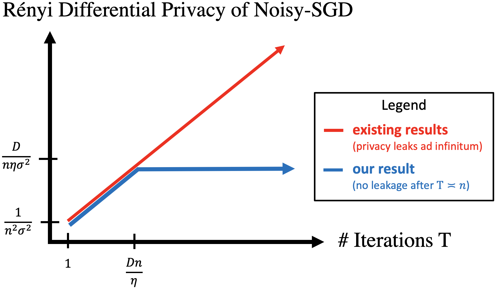
Figure 1: Even in the basic setting of smooth convex optimization over a bounded domain, existing implementations and theoretical analyses of Noisy-SGD—the standard algorithm for private optimization—leak privacy ad infinitum as the number of iterations $T$ increases. Our main result Theorem 1.3 establishes that after a small burn-in period of $\bar{T}\asymp n$ iterations, there is no further privacy loss. For simplicity, this plot considers Lipschitz parameter $L=1$ (wlog by rescaling), Rényi parameter $\alpha$ of constant size (the regime in practice), and omits logarithmic factors; see the main text for our precise (and optimal) dependence on all parameters.

Theorem 1.3 (Informal statement of main result: tight characterization of the privacy of Noisy-SGD).

For a large range of parameters, Noisy-SGD satisfies $(\alpha,\varepsilon)$-RDP for

$$\varepsilon\lesssim\frac{\alpha L^{2}}{n^{2}\sigma^{2}}\min\left\{T,\frac{Dn}{L\eta}\right\},$$ (1.2)

and moreover this bound is tight up to a constant factor.

Observe that the privacy bound in Theorem 1.3 is identical to the previous bound (1.1) when the number of iterations $T$ is small, but stops increasing when $T\geqslant\bar{T}$. Intuitively, $\bar{T}$ can be interpreted as the smallest number of iterations required for two SGD processes run on adjacent datasets to, with reasonable probability, reach opposite ends of the constraint set. In other words, $\bar{T}$ is effectively the smallest number of iterations before the final iterates could be maximally distinguishable.

To prove Theorem 1.3, we show a matching upper bound (in §3) and lower bound (in §4). These two bounds are formally stated as Theorems 3.1 and 4.1, respectively. See §1.3 for an overview of our techniques and how they depart from previous approaches.

We conclude this section with several remarks about Theorem 1.3.

Remark 1.4 (Tight DP characterization).

While Theorem 1.3 characterizes the privacy loss of Noisy-SGD in terms of RDP, our results can be restated in terms of standard DP bounds. Specifically, by a standard conversion from RDP to DP (Lemma 2.5), if $\delta$ is not smaller than exponentially small in $-b\sigma/n$ and if the resulting bound is $\varepsilon\lesssim 1$, it follows that Noisy-SGD is $(\varepsilon,\delta)$-DP for

$$\varepsilon\lesssim\frac{L}{n\sigma}\sqrt{\min\left\{T,\frac{Dn}{L\eta}\right\}\log 1/\delta}.$$ (1.3)

A matching DP lower bound, for the same large range of parameters as in Theorem 1.3, is proved along the way when we establish our RDP lower bound in §4.

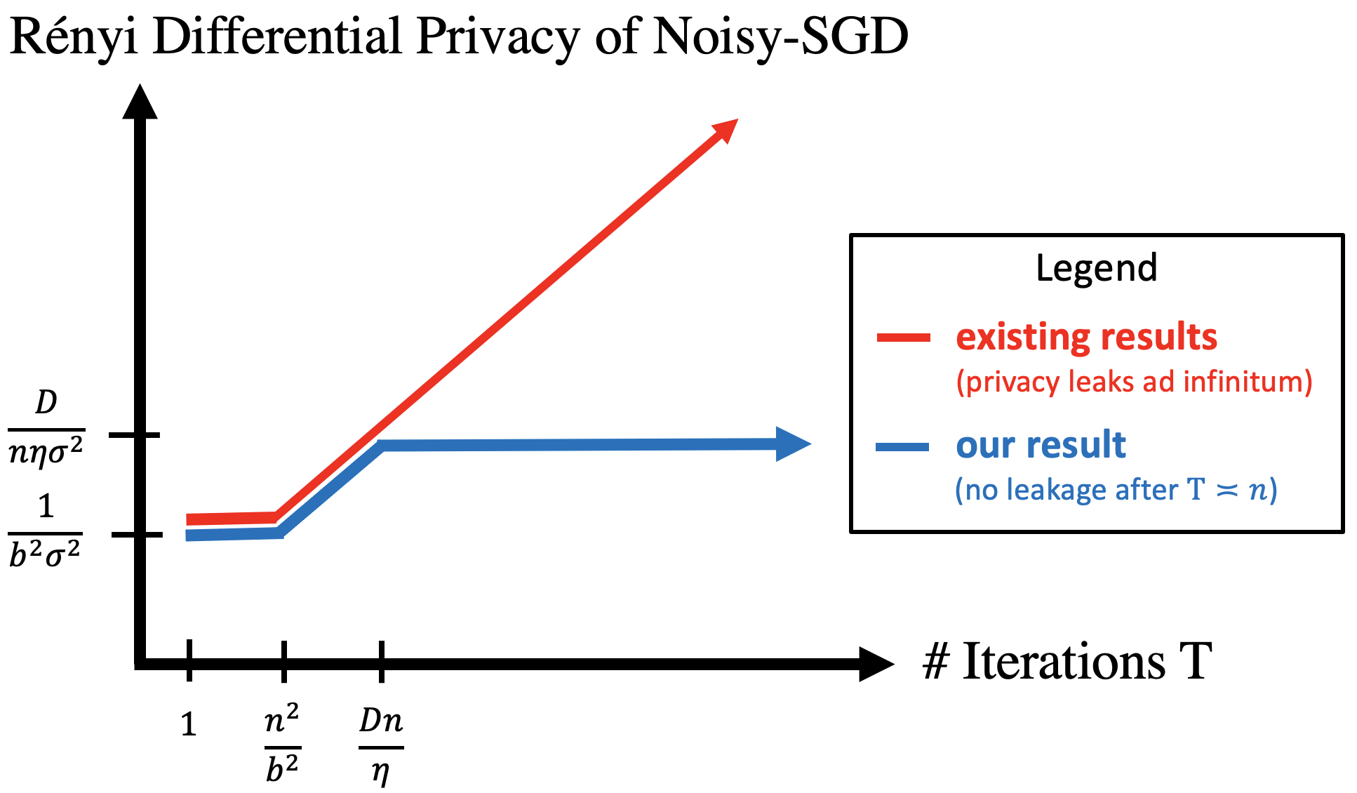
(a) In the setting of cyclic batch updates, the privacy of SGD is identical except for an unavoidable worsening in an initial phase (Theorem 5.8).

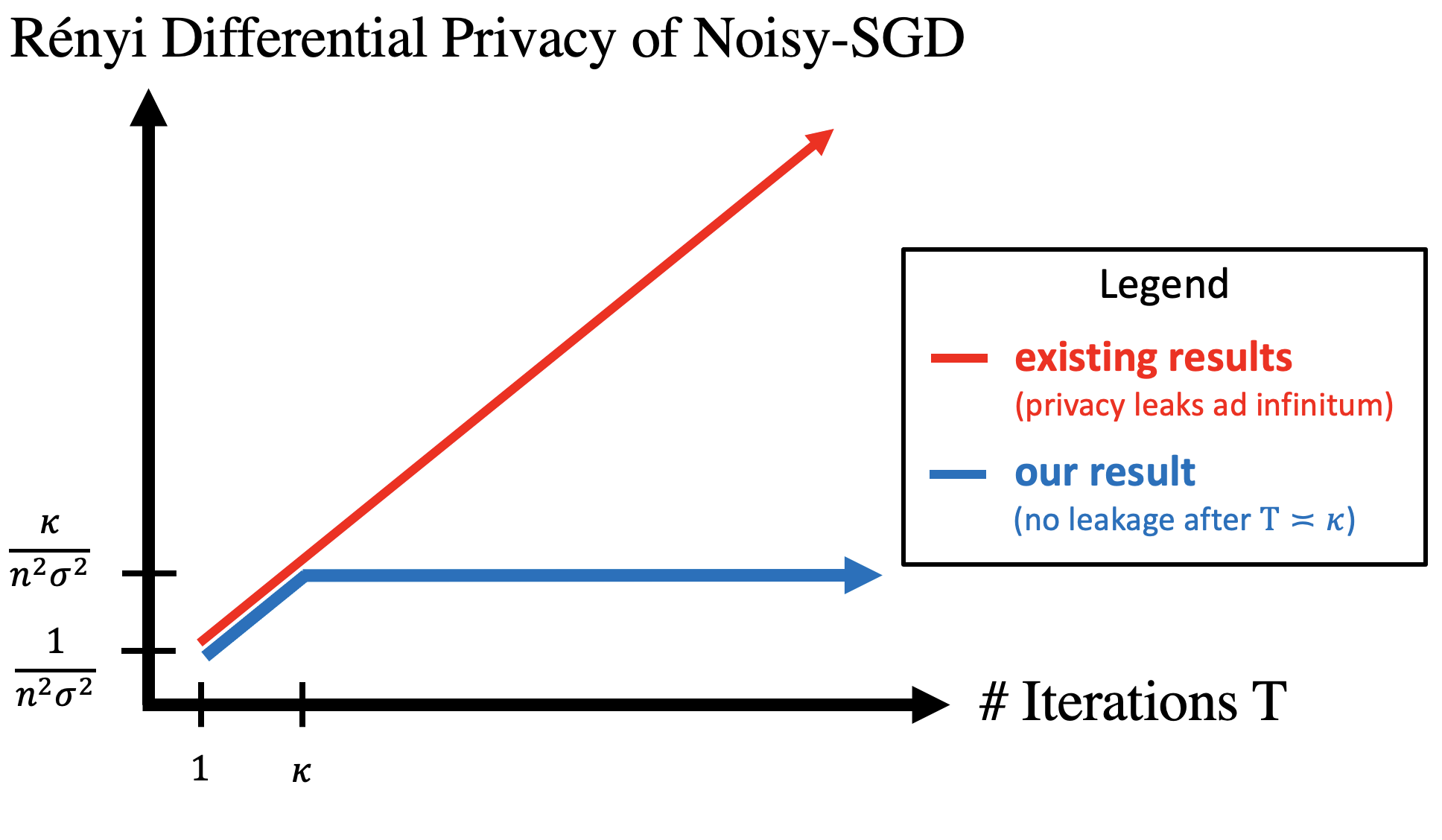
(b) In the setting of strongly convex losses, the privacy of Noisy-SGD is identical except the threshold $\bar{T}$ improves (Theorem 5.1). Plotted here for $\eta=1/M$.

Figure 2: Analog of Figure 1 for the extensions of our main result to other settings.

Discussion of extensions.

Our analysis techniques immediately extend to other settings:

• Strongly convex losses. If the convexity assumption on the losses is replaced by $m$-strong convexity, then Noisy-SGD enjoys better privacy. Specifically, the bound in Theorem 1.3 extends identially except that the threshold $\bar{T}$ for no further privacy loss improves from linear to logarithmic in $n$, namely $\tilde{O}(1/(\eta m))$. For example, if the stepsize $\eta=1/M$, then $\bar{T}=\tilde{O}(\kappa)$, where $\kappa=M/m$ denotes the condition number of the losses. This matches the independent results of [38, 47] (see Footnote 3) and uses completely different techniques from them. Details in §5.1; see also Figure 2(b) for an illustration of the privacy bound.

• Cyclic batch updates. Noisy-SGD is sometimes run with batches that are chosen cyclicallly rather than randomly. The bound in Theorem 1.3 extends identically, except for an initial transient phase in which there is unavoidably a large privacy loss since the algorithm may choose to update using a sensitive datapoint in an early batch. Details in §5.2; see also Figure 2(a) for an illustration of the privacy bound.

• Non-uniform stepsizes. Noisy-SGD is sometimes run with decaying stepsizes $\eta_{t}=t^{-c}$ for $c\in(0,1)$. The bound in Theorem 1.3 extends identically, with $\eta$ replaced by $\eta_{T}$. This means that the privacy increases after the threshold, but at the slower rate of $T^{c}\ll T$ for RDP (resp., $T^{c/2}\ll T^{1/2}$ for DP). Details in §5.3.

Discussion of assumptions.

• Boundedness. All previous privacy analyses are oblivious to any sort of diameter bound and therefore unavoidably increase ad infinitum, c.f. our lower bound in Theorem 1.3. Our analysis is the first to exploit boundedness: whereas previous analyses can only argue that having a smaller constraint set does not worsen the privacy loss, we show that this strictly improves the privacy loss, in fact making it convergent as $T\to\infty$. See the techniques section §1.3.

  We emphasize that this diameter bound is a mild constraint and is in common with all existing theoretical bounds for utility/optimization. Indeed, every utility guarantee for (non-strongly) convex losses also has a dependence on some similar diameter bound; this is inevitable simply due to the difference between the initialization and optimum. We also mention that one can solve an unconstrained problem by solving constrained problems with norm bounds, paying only a small logarithmic overhead on the number of solves and a constant overhead in the privacy loss using known techniques [29]. Moreover, in many optimization problems, the solution set is naturally constrained either from the problem formulation or application.

• Smoothness. The smoothness assumption on the losses can be relaxed if one runs Noisy-SGD on a smoothed version of the objective. This can be done using standard smoothing techniques, e.g., Gaussian convolution smoothing [19, §5.5], or Moreau-Yousida smoothing by replacing gradient steps with proximal steps [6, §4].

• Convexity. Convexity appears to be essential for privacy bounds that do not increase ad infinitum in $T$. Our analysis exploits convexity to ensure that Noisy-SGD is a contractive process. However, convexity is too restrictive when training deep networks, and it is an interesting question if the assumption of convexity can be relaxed. Any such result appears to require new techniques—if even true. The key challenge is that for any iterative process whose set of reachable fixed points is non-convex, there will be non-contractivity at the boundary between basins of attraction—and this appears to preclude arguments based on Privacy Amplification by Iteration, which at present is the only non-sampling-based technique with a hope of establishing convergent privacy bounds (see the techniques section §1.3).

• Lipschitzness. This assumption can be safely removed as the (necessary) assumptions of smoothness and bounded diameter already imply Lipschitzness (with parameter $L=MD$). We write our result in this way in order to isolate where this dependence comes from more simply, and also because the Lipschitz parameter $L$ may be much better than $MD$.

  Our analysis only uses Lipschitzness to bound gradient sensitivity, just like all previous analyses that use Privacy Amplification by Sampling. For details on this, as well as an example where gradient sensitivity is more useful in practice than Lipschitzness, see Section §5.4.

• Mild assumptions on parameters. The lower bound in Theorem 1.3 makes the mild assumption that the diameter $D$ of the decision set is asymptotically larger than both the movement size from one gradient step, and the standard deviation from $\bar{T}$ random increments of Gaussian noise $\mathcal{N}(0,\eta^{2}\sigma^{2})$ so that the noise does not overwhelm the learning.

  The upper bound uses the technique of Privacy Amplification by Sampling, and thus inherits two mild assumptions on the parameters that are also inherent in all previous analyses of Noisy-SGD. One is an upper bound assumption on $\alpha$, and the other is a lower bound assumption on the noise $\sigma$ so that one step of Noisy-SGD provides at least constant privacy to any user. These restrictions neither affect numerical bounds which can be computed for any $\alpha$ and $\sigma$ (see §2.3), nor do they affect the asymptotic $(\varepsilon,\delta)$-DP bounds in most parameter regimes of interest. We also remark that our results require no restriction if the batches are chosen cyclically, and thus also if full-batch gradients are used (see Theorem 5.8).

1.3 Techniques

Upper bound on privacy.

Our analysis technique departs from recent approaches based on fast mixing. This allows us to bypass the many longstanding technical challenges discussed in §1.1.

Instead, our analysis combines the techniques of Privacy Amplification by Iteration and Privacy Amplification by Sampling. As discussed in §1.1, previous analyses based on these techniques yield loose privacy bounds that increase ad infinitum in $T$. Indeed, bounds based on Privacy Amplification by Sampling inevitably diverge since they “pay” for releasing the entire sequence of $T$ iterates, each of which leaks more information about the private data [5, 2]. Privacy Amplification by Iteration avoids releasing the entire sequence by directly arguing about the final iterate; however, previous arguments based on this technique are unable to exploit a diameter bound on the constraint set, and therefore inevitably lead to privacy bounds which grow unboundedly in $T$ [19].

Our analysis hinges on the observation that when the iterates are constrained to a bounded domain, we can combine the techniques of Privacy Amplification by Iteration and Privacy Amplification by Sampling in order to only pay for the privacy loss from the final $\bar{T}\asymp(Dn)/(L\eta)$ iterations. To explain this, first recall that by definition, differential privacy of Noisy-SGD means that the final iterate of Noisy-SGD is similar when run on two (adjacent but) different datasets from the same initialization. At an intuitive level, we establish this by arguing about the privacy of the following three scenarios:

• Run Noisy-SGD for $T$ iterations on different datasets from same initialization.

• Run Noisy-SGD for $\bar{T}$ iterations on different datasets from different initializations.

• Run Noisy-SGD for $\bar{T}$ iterations on same datasets from different initializations.

In order to analyze (i), which as mentioned is the definition of Noisy-SGD being differentially private, we argue that no matter how different the two input datasets are, the two Noisy-SGD iterates at iteration $T-\bar{T}$ are within distance $D$ of each other since they lie within the constraint set $\mathcal{K}$ of diameter $D$. Thus in particular, the privacy of scenario (i) is at most the privacy of scenario (ii), which has initializations that can be arbitrarily different so long as they are within distance $D$ from each other. In this way, we arrive at a scenario which is independent of $T$. This is crucial for obtaining privacy bounds which do not diverge in $T$; however, previously privacy analyses could not proceed in this way because they could not argue about different initialization.

In order to analyze (ii), we use the technique of Privacy Amplification by Sampling—but only on these final $\bar{T}\ll T$ iterations. In words, this enables us to argue that the noisy gradients that Noisy-SGD uses in the last $\bar{T}$ iterations are indistinguishable up to a certain privacy loss (to be precise the RDP scales linearly in $\bar{T}$) despite the fact that they are computed on different input datasets. This enables us to reduce analyzing the privacy of scenario (ii) to scenario (iii).

In order to analyze (iii), we use a new diameter-aware version of Privacy Amplification by Iteration (Proposition 3.2). In words, this shows that running the same Noisy-SGD updates on two different initializations masks their initial difference due to both the noise and contraction maps that define each Noisy-SGD update. Of course, this indistinguishability improves the longer that Noisy-SGD is run (to be precise, we show that the RDP scales inversely in $\bar{T}$).

We arrive, therefore, at a privacy loss which is the sum of the bounds from the Privacy Amplification by Sampling argument in step (ii) and the Privacy Amplification by Iteration argument in step (iii). This privacy loss has a natural tradeoff in the parameter $\bar{T}$: the former bound leads to a privacy loss that increases in $\bar{T}$ (since it pays for the release of $\bar{T}$ noisy gradients), whereas the latter bound leads to a privacy loss that decreases in $\bar{T}$ (since more iterations of the same Noisy-SGD process enable better masking of different initializations). Balancing these two privacy bounds leads to the final choice $\bar{T}\asymp\tfrac{Dn}{L\eta}$. (We remark that this quantity is not just an artefact of our analysis, but in fact is the true answer for when the privacy loss stops increasing, as established by our matching lower bound.)

At a high-level, our analysis proceeds by carefully running these arguments in parallel.

We emphasize that this analysis is the first to show that the privacy loss of Noisy-SGD can strictly improve if the constraint set is made smaller. In contrast, previous analyses only argue that restricting the constraint set cannot worsen the privacy loss (e.g., by using a post-processing inequality to analyze the projection step). The key technical challenge in exploiting a diameter bound is dealing with the complicated non-linearities that arise when interleaving projections with noisy gradient updates. Our techniques enable such an analysis.

Lower bound on privacy.

We construct two adjacent datasets for which the corresponding Noisy-SGD processes are random walks—one symmetric, one biased—that are confined to an interval of length $D$. In this way, we reduce the question of how large is the privacy loss of Noisy-SGD, to the question of how distinguishable is a constrained symmetric random walk from a constrained biased random walk. The core technical challenge is that the distributions of the iterates of these random walks are intractable to reason about explicitly—due to the highly non-linear interactions between the projections and random increments. Briefly, our key technique here is a way to modify these processes so that on one hand, their distinguishability is essentially the same, and the other hand, no projections occur with high probability—allowing us to explicitly compute their distributions and thus also their distinguishability. Details in §4.

1.4 Other related work

Private sampling.

The mixing time of (stochastic) Langevin Dynamics has been extensively studied in recent years starting with [13, 15]. A recent focus in this vein is analyzing mixing in more stringent notions of distance, such as the Rényi divergence [43, 22], in part because this is necessary for proving privacy bounds. In addition to the aforementioned results, several other works focus on sampling from the distribution $\exp(\varepsilon\sum_{i}f_{i}(\omega)$ or its regularized versions from a privacy viewpoint. [31] proposed a mechanism of this kind that works for unbounded $f$ and showed $(\varepsilon,\delta)$-DP. Recently, [24] gave better privacy bounds for such a regularized exponential mechanism, and designed an efficient sampler based only on function evaluation. Also, [23] showed that the continuous Langevin Diffusion has optimal utility bounds for various private optimization problems.

As alluded to in §1.1, there are several core issues with trying to prove DP bounds for Noisy-SGD by directly combining “fast mixing” bounds with “private once mixed” bounds. First, mixing results typically do not apply, e.g., since DP requires mixing in stringent divergences like Rényi, or because realistic settings with constraints, stochasticity, and lack of strong convexity are difficult to analyze—indeed, understanding the mixing time for such settings is a challenging open problem. Second, even when fast mixing bounds do apply, directly combining them with “private once mixed” bounds unavoidably leads to DP bounds that are loose to the point of being essentially useless (e.g., the inevitable dimension dependence in mixing bounds to the stationary distribution of the continuous-time Langevin Diffusion would lead to dimension dependence in DP bounds, which should not occur—as we show). Third, even if a Markov chain were private after mixing, one cannot conclude from this that it is private beforehand—indeed, there are simple Markov chains which are private after mixing, yet are exponentially non-private beforehand [21].

Utility bounds.

In the field of private optimization, one separately analyzes two properties of algorithms: (i) the privacy loss as a function of the number of iterations, and (ii) the utility (a.k.a., optimization error) as a function of the number of iterations. These two properties can then be combined to obtain privacy-utility tradeoffs. The purpose of this paper is to completely resolve (i); this result can then be combined with any bound on (ii).

Utility bounds for SGD are well understood [39], and these analyses have enabled understanding utility bounds for Noisy-SGD in empirical [5] and population [6] settings. However, there is a big difference between the minimax-optimal utility bounds in theory versus what is desired in practice. Indeed, while in theory a single pass of Noisy-SGD achieves the minimax-optimal population risk [20], in practice Noisy-SGD benefits from running longer to get more accurate training. In fact, this divergence is even true and well-documented for non-private SGD as well, where one epoch is minimax-optimal in theory, but in practice more epochs help. Said simply, this is because typical problems are not worst-case problems (i.e., minimax-optimal theoretical bounds are typically not representative of practice). For these practical settings, in order to run Noisy-SGD longer, it is essential to have privacy bounds which do not increase ad infinitum. Our paper resolves this.

1.5 Organization

Section 2 recalls relevant preliminaries. Our main result Theorem 1.3 is proved in Section 3 (upper bound) and Section 4 (lower bound). Section 5 contains extensions to strongly convex losses, cyclic batch updates, and non-uniform stepsizes. §6 concludes with future research directions motivated by these results. For brevity, several proofs are deferred to Appendix A. For simplicity, we do not optimize constants in the main text; this is done in Appendix B.

2 Preliminaries

In this section, we recall relevant preliminaries about convex optimization (§2.1), differential privacy (§2.2), and two by-now-standard techniques for analyzing the privacy of optimization algorithms—namely, Privacy Amplification by Sampling (§2.3) and Privacy Amplification by Iteration (§2.4).

Notation.

We write $\mathbb{P}_{X}$ to denote the law of a random variable $X$, and $\mathbb{P}_{X|Y=y}$ to denote the law of $X$ given the event $Y=y$. We write $Z_{S:T}$ as shorthand for the vector concatenating $Z_{S},\dots,Z_{T}$. We write $f_{\#}\mu$ to denote the pushforward of a distribution $\mu$ under a function $f$, i.e., the law of $f(X)$ where $X\sim\mu$. We abuse notation slightly by writing $f_{\#}\mu$ even when $f$ is a “random function”, by which we mean a Markov transition kernel. We write $\mu\ast\nu$ to denote the convolution of probability distributions $\mu$ and $\nu$, i.e., the law of $X+Y$ where $X\sim\mu$ and $Y\sim\nu$ are independently distributed. We write $\lambda\mu+(1-\lambda)\nu$ to denote the mixture distribution that is $\mu$ with probability $\lambda$ and $\nu$ with probability $1-\lambda$. We write $\mathcal{A}(\mathcal{X})$ to denote the output of an algorithm $\mathcal{A}$ run on input $\mathcal{X}$; this is a probability distribution if $\mathcal{A}$ is a randomized algorithm.

2.1 Convex optimization

Throughout, the loss function corresponding to a data point $x_{i}$ or $x_{i}^{\prime}$ is denoted by $f_{i}$ or $f_{i}^{\prime}$, respectively. While the dependence on the data point is arbitrary, the loss functions are assumed to be convex in the argument $\omega\in\mathcal{K}$ (a.k.a., the machine learning model we seek to train). Throughout, the set $\mathcal{K}$ of possible models is a convex subset of $\mathbb{R}^{d}$. In order to establish both optimization and privacy guarantees, two additional assumptions are required on the loss functions. Recall that a differentiable function $g:\mathcal{K}\to\mathbb{R}^{d}$ is said to be:

• $L$-Lipschitz if $\|g(\omega)-g(\omega^{\prime})\|\leqslant L\|\omega-\omega^{\prime}\|$ for all $\omega,\omega^{\prime}\in\mathcal{K}$.

• $M$-smooth if $\|\nabla g(\omega)-\nabla g(\omega^{\prime})\|\leqslant M\|\omega-\omega^{\prime}\|$ for all $\omega,\omega^{\prime}\in\mathcal{K}$.

An important implication of smoothness is the following well-known fact; for a proof, see e.g., [35].

Lemma 2.1 (Small gradient steps on smooth convex losses are contractions).

Suppose $f:\mathbb{R}^{d}\to\mathbb{R}$ is a convex, $M$-smooth function. For any $\eta\leqslant 2/M$, the mapping $\omega\mapsto\omega-\eta\nabla f(\omega)$ is a contraction.

2.2 Differential privacy and Rényi differential privacy

Over the past two decades, differential privacy (DP) has become a standard approach for quantifying how much sensitive information an algorithm leaks about the dataset it is run upon. Differential privacy was first proposed in [17], and is now widely used in industry (e.g., at Apple [36], Google [18], Microsoft [14], and LinkedIn [37]), as well as in government data collection such as the 2020 US Census [44]. In words, DP measures how distinguishable the output of an algorithm is when run on two “adjacent” datasets—i.e., two datasets which differ on at most one datapoint.

Definition 2.2 (Differential Privacy).

A randomized algorithm $\mathcal{A}$ satisfies $(\varepsilon,\delta)$-DP if for any two adjacent datasets $\mathcal{X},\mathcal{X}^{\prime}$ and any measurable event $S$,

$$\mathbb{P}\left[\mathcal{A}(\mathcal{X})\in S\right]\leqslant e^{\varepsilon}\mathbb{P}\left[\mathcal{A}(\mathcal{X}^{\prime})\in S\right]+\delta.$$

In order to prove DP guarantees, we work with the related notion of Rényi Differential Privacy (RDP) introduced by [32], since RDP is more amenable to our analysis techniques and is readily converted to DP guarantees. To define RDP, we first recall the definition of Rényi divergence.

Definition 2.3 (Rényi divergence).

The Rényi divergence between two probability measures $\mu$ and $\nu$ of order $\alpha\in(1,\infty)$ is

$$\mathcal{D}_{\alpha}\left(\mu\;\|\;\nu\right)=\frac{1}{\alpha-1}\log\int\left(\frac{\mu(x)}{\nu(x)}\right)^{\alpha}\nu(x)dx,$$

if $\mu\ll\nu$, and is $\infty$ otherwise. Here we adopt the standard convention that $0/0=0$ and $x/0=\infty$ for $x>0$. The Rényi divergences of order $\alpha\in\{1,\infty\}$ are defined by continuity.

Definition 2.4 (Rényi Differential Privacy).

A randomized algorithm $\mathcal{A}$ satisfies $(\alpha,\varepsilon)$-RDP if for any two adjacent datasets $\mathcal{X},\mathcal{X}^{\prime}$,

$$\mathcal{D}_{\alpha}\left(\mathcal{A}(\mathcal{X})\;\|\;\mathcal{A}(\mathcal{X}^{\prime})\right)\leqslant\varepsilon.$$

It is straightforward to convert an RDP bound to a DP bound as follows [32, Proposition 1].

Lemma 2.5 (RDP-to-DP conversion).

Suppose that an algorithm satisfies $(\alpha,\varepsilon_{\alpha})$-RDP for some $\alpha>1$. Then the algorithm satisfies $(\varepsilon_{\delta},\delta)$-DP for any $\delta\in(0,1)$ and $\varepsilon_{\delta}=\varepsilon_{\alpha}+(\operatorname{\log\tfrac{1}{\delta}})/(\alpha-1)$.

Following, we recall three basic properties of RDP that we use repeatedly in our analysis. The first property regards convexity. While the KL divergence (the case $\alpha=1$) is jointly convex in its two arguments, for $\alpha\neq 1$ the Rényi divergence is only jointly quasi-convex. See e.g., [42, Theorem 13] for a proof and a further discussion of partial convexity properties of the Rényi divergence.

Lemma 2.6 (Joint quasi-convexity of Rényi divergence).

For any Rényi parameter $\alpha\geqslant 1$, any mixing probability $\lambda\in[0,1]$, and any two pairs of probability distributions $\mu,\nu$ and $\mu^{\prime},\nu^{\prime}$,

$$\mathcal{D}_{\alpha}\left(\lambda\mu+(1-\lambda)\mu^{\prime}\;\|\;\lambda\nu+(1-\lambda)\nu^{\prime}\right)\leqslant\max\left\{\mathcal{D}_{\alpha}\left(\mu\;\|\;\nu\right),\mathcal{D}_{\alpha}\left(\mu^{\prime}\;\|\;\nu^{\prime}\right)\right\}.$$

The second property states that pushing two measures forward through the same (possibly random) function cannot increase the Rényi divergence. This is the direct analog of the classic “data-processing inequality” for the KL divergence. See e.g., [42, Theorem 9] for a proof.

Lemma 2.7 (Post-processing property of Rényi divergence).

For any Rényi parameter $\alpha\geqslant 1$, any (possibly random) function $h$, and any probability distributions $\mu,\nu$,

$$\mathcal{D}_{\alpha}\left(h_{\#}\mu\;\|\;h_{\#}\nu\right)\leqslant\mathcal{D}_{\alpha}\left(\mu\;\|\;\nu\right).$$

The third property is the appropriate analog of the chain rule for the KL divergence (the direct analog of the chain rule does not hold for Rényi divergences, $\alpha\neq 1$). This bound has appeared in various forms in previous work (e.g., [2, 32, 16]); we state the following two equivalent versions of this bound since at various points in our analysis it will be more convenient to reference one or the other. A proof of the former version is in [32, Proposition 3]. The proof of the latter is similar to [2, Theorem 2]; for the convenience of the reader, we provide a brief proof in Section A.1.

Lemma 2.8 (Strong composition for RDP, v1).

Suppose algorithms $\mathcal{A}_{1}$ and $\mathcal{A}_{2}$ satisfy $(\alpha,\varepsilon_{1})$-RDP and $(\alpha,\varepsilon_{2})$-RDP, respectively. Let $\mathcal{A}$ denote the algorithm which, given a dataset $\mathcal{X}$ as input, outputs the composition $\mathcal{A}(\mathcal{X})=(\mathcal{A}_{1}(\mathcal{X}),\mathcal{A}_{2}(\mathcal{X},\mathcal{A}_{1}(\mathcal{X})))$. Then $\mathcal{A}$ satisfies $(\alpha,\varepsilon_{1}+\varepsilon_{2})$-RDP.

Lemma 2.9 (Strong composition for RDP, v2).

For any Rényi parameter $\alpha\geqslant 1$ and any two sequences of random variables $X_{1},\dots,X_{k}$ and $Y_{1},\dots,Y_{k}$,

$$\mathcal{D}_{\alpha}\left(\mathbb{P}_{X_{1:k}}\,\big{\|}\,\mathbb{P}_{Y_{1:k}}\right)\leqslant\sum_{i=1}^{k}\sup_{x_{1:i-1}}\mathcal{D}_{\alpha}\left(\mathbb{P}_{X_{i}|X_{1:i-1}=x_{1:i-1}}\;\|\;\mathbb{P}_{Y_{i}|Y_{1:i-1}=x_{1:i-1}}\right).$$

2.3 Privacy Amplification by Sampling

A core technique in the DP literature is Privacy Amplification by Sampling [27] which quantifies the idea that a private algorithm, run on a small random sample of the input, becomes more private. There are several ways of formalizing this. For our purpose of analyzing Noisy-SGD, we must understand how distinguishable a noisy stochastic gradient update is when run on two adjacent datasets. This is precisely captured by the “Sampled Gaussian Mechanism”, which is a composition of two operations: subsampling and additive Gaussian noise. Below we recall a convenient statement of this in terms of RDP from [33]. We start with a preliminary definition in one dimension.

Definition 2.10 (Rényi Divergence of the Sampled Gaussian Mechanism).

For Rényi parameter $\alpha\geqslant 1$, mixing probability $q\in(0,1)$, and noise parameter $\sigma>0$, define

$$S_{\alpha}(q,\sigma):=\mathcal{D}_{\alpha}\left(\mathcal{N}(0,\sigma^{2})\,\big{\|}\,(1-q)\mathcal{N}(0,\sigma^{2})+q\mathcal{N}(1,\sigma^{2})\right).$$

Next, we provide a simple lemma that extends this notion to higher dimensions. In words, the proof simply argues that the worst-case distribution $\mu$ is a Dirac supported on a point of maximal norm, and then reduces the multivariate setting to the univariate setting via rotational invariance. The proof is similar to [33, Theorem 4]; for convenience, details are provided in Section A.2.

Lemma 2.11 (Extrema for Rényi Divergence of the Sampled Gaussian Mechanism).

For any Rényi parameter $\alpha\geqslant 1$, mixing probability $q\in(0,1)$, noise level $\sigma>0$, dimension $d\in\mathbb{N}$, and radius $R>0$,

$$\sup_{\mu\in\mathcal{P}(R\mathbb{B}_{d})}\mathcal{D}_{\alpha}\left(\mathcal{N}(0,\sigma^{2}I_{d})\,\big{\|}\,(1-q)\mathcal{N}(0,\sigma^{2}I_{d})+q\left(\mathcal{N}(0,\sigma^{2}I_{d})\ast\mu\right)\right)=S_{\alpha}(q,\sigma/R),$$

where above $\mathcal{P}(R\mathbb{B}_{d})$ denotes the set of Borel probability distributions that are supported on the ball of radius $R$ in $\mathbb{R}^{d}$.

Finally, we recall the tight bound [33, Theorem 11] on these quantities. This bound restricts to Rényi parameter at most $\alpha^{*}(q,\sigma)$, which is defined to be the largest $\alpha$ satisfying $\alpha\leqslant M\sigma^{2}/2-\log(\sigma^{2})$ and $\alpha\leqslant(M^{2}\sigma^{2}/2-\log(5\sigma^{2}))/(M+\log(q\alpha)+1/(2\sigma^{2}))$, where $M=\log(1+1/(q(\alpha-1)))$. While we use Lemma 2.12 to prove the asymptotics in our theoretical results, we emphasize that i) our bounds can be computed numerically for any $\alpha\geqslant 1$, see Remark B.1; and ii) this upper bound does not preclude $\alpha$ from the typical parameter regime of interest, see the discussion in §1.2.

Lemma 2.12 (Bound on Rényi Divergence of the Sampled Gaussian Mechanism).

Consider Rényi parameter $\alpha>1$, mixing probability $q\in(0,1/5)$, and noise level $\sigma\geqslant 4$. If $\alpha\leqslant\alpha^{*}(q,\sigma)$, then

$$S_{\alpha}(q,\sigma)\leqslant 2\alpha q^{2}/\sigma^{2}.$$

2.4 Privacy Amplification by Iteration

The Privacy Amplification by Iteration technique of [19] bounds the privacy loss of an iterative algorithm without “releasing” the entire sequence of iterates—unlike arguments based on Privacy Amplification by Sampling, c.f., the discussion in §1.3. This technique applies to processes which are generated by a Contractive Noisy Iteration (CNI). We begin by recalling this definition, albeit in a slightly more general form that allows for two differences. The first difference is allowing the contractions to be random; albeit simple, this generalization is critical for analyzing Noisy-SGD because a stochastic gradient update is random. The second difference is that we project each iterate; this generalization is solely for convenience as it simplifies the exposition.

Definition 2.13 (Contractive Noisy Iteration).

Consider a (random) initial state $X_{0}\in\mathbb{R}^{d}$, a sequence of (random) contractions $\phi_{t}:\mathbb{R}^{d}\to\mathbb{R}^{d}$, a sequence of noise distributions $\xi_{t}$, and a convex set $\mathcal{K}$. The Projected Contractive Noisy Iteration $\mathrm{CNI}(X_{0},\{\phi_{t}\},\{\xi_{t}\},\mathcal{K})$ is the law of the final iterate $X_{T}$ of the process

$$X_{t+1}=\Pi_{\mathcal{K}}\left[\phi_{t+1}(X_{t})+Z_{t+1}\right],$$

where $Z_{t+1}$ is drawn independently from $\xi_{t+1}$.

Privacy Amplification by Iteration is based on two key lemmas. We recall both below in the case of Gaussian noise since this suffices for our purposes. We begin with a preliminary definition.

Definition 2.14 (Shifted Rényi Divergence; Definition 8 of [19]).

Let $\mu,\nu$ be probability distributions over $\mathbb{R}^{d}$. For parameters $z\geqslant 0$ and $\alpha\geqslant 1$, the shifted Rényi divergence is

$$\mathcal{D}_{\alpha}^{(z)}\big{(}\mu\;\|\;\nu\big{)}=\inf_{\mu^{\prime}\;:\;W_{\infty}(\mu,\mu^{\prime})\leqslant z}\mathcal{D}_{\alpha}\big{(}\mu^{\prime}\;\|\;\nu\big{)}.$$

(Recall that the $\infty$-Wasserstein metric $\mathcal{W}_{\infty}(\mu,\mu^{\prime})$ between two distributions $\mu$ and $\mu^{\prime}$ is the smallest real number $w$ for which the following holds: there exists a joint distribution $\mathbb{P}_{X,X^{\prime}}$ with first marginal $X\sim\mu$ and second marginal $X^{\prime}\sim\mu^{\prime}$, under which $\|X-X^{\prime}\|\leqslant w$ almost surely.)

The shift-reduction lemma [19, Lemma 20] bounds the shifted Rényi divergence between two distributions that are convolved with Gaussian noise.

Lemma 2.15 (Shift-reduction lemma).

Let $\mu,\nu$ be probability distributions on $\mathbb{R}^{d}$. For any $a\geqslant 0$,

$$\mathcal{D}_{\alpha}^{(z)}\left(\mu\ast\mathcal{N}(0,\sigma^{2}I_{d})\;\big{\|}\;\nu\ast\mathcal{N}(0,\sigma^{2}I_{d})\right)\leqslant\mathcal{D}_{\alpha}^{(z+a)}\left(\mu\;\big{\|}\;\nu\right)+\frac{\alpha a^{2}}{2\sigma^{2}}.$$

The contraction-reduction lemma [19, Lemma 21] bounds the shifted Rényi divergence between the pushforwards of two distributions through similar contraction maps. Below we state a slight generalization of [19, Lemma 21] that allows for random contraction maps. The proof of this generalization is similar, except that here we exploit the quasi-convexity of the Rényi divergence to handle the additional randomness; details in Section A.3.

Lemma 2.16 (Contraction-reduction lemma, for random contractions).

Suppose $\phi,\phi^{\prime}$ are random functions from $\mathbb{R}^{d}$ to $\mathbb{R}^{d}$ such that (i) each is a contraction almost surely; and (ii) there exists a coupling of $(\phi,\phi^{\prime})$ under which $\sup_{z}\|\phi(z)-\phi^{\prime}(z)\|\leqslant s$ almost surely. Then for any probability distributions $\mu$ and $\mu^{\prime}$ on $\mathbb{R}^{d}$,

$$\mathcal{D}_{\alpha}^{(z+s)}\left(\phi_{\#}\mu\|\phi_{\#}^{\prime}\mu^{\prime}\right)\leqslant\mathcal{D}_{\alpha}^{(z)}\left(\mu\|\mu^{\prime}\right).$$

The original Privacy Amplification by Iteration argument combines these two lemmas to establish the following bound.

Proposition 2.17 (Original PABI bound).

Let $X_{T}$ and $X_{T}^{\prime}$ denote the outputs of $\mathrm{CNI}(X_{0},\{\phi_{t}\},\{\xi_{t}\},\mathcal{K})$ and $\mathrm{CNI}(X_{0},\{\phi_{t}^{\prime}\},\{\xi_{t}\},\mathcal{K})$ where $\xi_{t}=\mathcal{N}(0,\sigma_{t}^{2}I_{d})$. Let $s_{t}:=\sup_{x}\|\phi_{t}(x)-\phi_{t}^{\prime}(x)\|$, and consider any sequence $a_{1},\dots,a_{T}$ such that $z_{t}:=\sum_{i=1}^{t}(s_{i}-a_{i})$ is non-negative for all $t$ and satisfies $z_{T}=0$. Then

$$\mathcal{D}_{\alpha}\left(\mathbb{P}_{X_{T}}\;\|\;\mathbb{P}_{X_{T}^{\prime}}\right)\leqslant\frac{\alpha}{2}\sum_{t=1}^{T}\frac{a_{t}^{2}}{\sigma_{t}^{2}}.$$

3 Upper bound on privacy

In this section, we prove the upper bound in Theorem 1.3. The formal statement of this result is as follows; see §1.2 for a discussion of the mild assumptions on $\sigma$ and $\alpha$.

Theorem 3.1 (Privacy upper bound for Noisy-SGD).

Let $\mathcal{K}\subset\mathbb{R}^{d}$ be a convex set of diameter $D$, and consider optimizing convex losses over $\mathcal{K}$ that are $L$-Lipschitz and $M$-smooth. For any number of iterations $T$, dataset size $n\in\mathbb{N}$, batch size $b\leqslant n$, stepsize $\eta\leqslant 2/M$, noise parameter $\sigma>8\sqrt{2}L/b$, and initialization $\omega_{0}\in\mathcal{K}$, Noisy-SGD satisfies $(\alpha,\varepsilon)$-RDP for $1<\alpha\leqslant\alpha^{*}(\tfrac{b}{n},\tfrac{b\sigma}{2\sqrt{2}L})$ and

$$\varepsilon\lesssim\frac{\alpha L^{2}}{n^{2}\sigma^{2}}\min\left\{T,\bar{T}\right\}\,,$$

where $\bar{T}:=\lceil\frac{Dn}{L\eta}\rceil$.

Below, in §3.1 we first isolate a simple ingredient in our analysis as it may be of independent interest. Then in §3.2 we prove Theorem 3.1.

3.1 Privacy Amplification by Iteration bounds that are not vacuous as $T\to\infty$

Recall from the preliminaries section §2.4 that Privacy Amplification by Iteration arguments, while tight for a small number of iterations $T$, provide vacuous bounds as $T\to\infty$ (c.f., Proposition 2.17). The following proposition overcomes this by establishing privacy bounds which are independent of the number of iterations $T$. This result only requires additionally assuming that $\|X_{\tau}-X_{\tau}^{\prime}\|$ is bounded at some intermediate time $\tau$. This is a mild assumption that is satisfied automatically if, e.g., both CNI processes are in a constraint set of bounded diameter.

Proposition 3.2 (New PABI bound that is not vacuous as $T\to\infty$).

Let $X_{T}$, $X_{T}^{\prime}$, and $s_{t}$ be as in Proposition 2.17. Consider any $\tau\in\{0,\dots,T-1\}$ and sequence $a_{\tau+1},\dots,a_{T}$ such that $z_{t}:=D+\sum_{i=\tau+1}^{t}(s_{i}-a_{i})$ is non-negative for all $t$ and satisfies $z_{T}=0$. If $\mathcal{K}$ has diameter $D$, then:

$$\mathcal{D}_{\alpha}\left(\mathbb{P}_{X_{T}}\;\|\;\mathbb{P}_{X_{T}^{\prime}}\right)\leqslant\frac{\alpha}{2}\sum_{t=\tau+1}^{T}\frac{a_{t}^{2}}{\sigma_{t}^{2}}.$$

In words, the main idea behind Proposition 3.2 is simply to change the original Privacy Amplification by Iteration argument—which bounds the shifted divergence at iteration $T$, by the shifted divergence at iteration $T-1$, and so on all the way to the shifted divergence at iteration $0$—by instead stopping the induction earlier. Specifically, only unroll to iteration $\tau$, and then use boundedness of the iterates to control the shifted divergence at that intermediate time $\tau$.

We remark that this new version of PABI uses the shift in the shifted Rényi divergence for a different purpose than previous work: rather than just using the shift to bound the bias incurred from updating on two different losses, here we also use the shift to exploit the boundedness of the constraint set.

Proof of Proposition 3.2.

Bound the divergence at iteration $T$ by the shifted divergence at iteration $T-1$ as follows:

$$\mathcal{D}_{\alpha}\left(\mathbb{P}_{X_{T}}\;\|\;\mathbb{P}_{X_{T}^{\prime}}\right) =\mathcal{D}_{\alpha}^{(z_{T})}\left(\mathbb{P}_{X_{T}}\;\|\;\mathbb{P}_{X_{T}^{\prime}}\right)$$

$$=\mathcal{D}_{\alpha}^{(z_{T-1}+s_{T}-a_{T})}\left(\mathbb{P}_{\Pi_{\mathcal{K}}[\phi_{T}(X_{T-1})+Z_{T}]}\;\|\;\mathbb{P}_{\Pi_{\mathcal{K}}[\phi_{T-1}^{\prime}(X_{T-1}^{\prime})+Z_{T}^{\prime}}]\right)$$

$$\leqslant\mathcal{D}_{\alpha}^{(z_{T-1}+s_{T}-a_{T})}\left(\mathbb{P}_{\phi_{T}(X_{T-1})+Z_{T}}\;\|\;\mathbb{P}_{\phi_{T-1}^{\prime}(X_{T-1}^{\prime})+Z_{T}^{\prime}}\right)$$

$$\leqslant\mathcal{D}_{\alpha}^{(z_{T-1}+s_{T})}\left(\mathbb{P}_{\phi_{T}(X_{T-1})}\;\|\;\mathbb{P}_{\phi_{T-1}^{\prime}(X_{T-1}^{\prime})}\right)+\frac{\alpha a_{T}^{2}}{2\sigma_{T}^{2}}$$

$$\leqslant\mathcal{D}_{\alpha}^{(z_{T-1})}\left(\mathbb{P}_{X_{T-1}}\;\|\;\mathbb{P}_{X_{T-1}}^{\prime}\right)+\frac{\alpha a_{T}^{2}}{2\sigma_{T}^{2}}.$$

Above, the first step is because $z_{T}=0$; the second step is by the iterative construction of $X_{T},X_{T}^{\prime},z_{T}$; the third and final steps are by the the contraction-reduction lemma (Lemma 2.16), and the penulimate step is by the shift-reduction lemma (Lemma 2.15).

By repeating the above argument, from $T$ to $T-1$ all the way to $\tau$, we obtain:

$$\mathcal{D}_{\alpha}\left(\mathbb{P}_{X_{T}}\;\|\;\mathbb{P}_{X_{T}^{\prime}}\right)\leqslant\mathcal{D}_{\alpha}^{(z_{\tau})}\left(\mathbb{P}_{X_{\tau}}\;\|\;\mathbb{P}_{X_{\tau}}^{\prime}\right)+\frac{\alpha}{2}\sum_{t=\tau+1}^{T}\frac{a_{t}^{2}}{\sigma_{t}^{2}}.$$

Now observe that the shifted Rényi divergence on the right hand side vanishes because $z_{\tau}=D$. ∎

3.2 Proof of Theorem 3.1

Step 1: Coupling the iterates

Suppose $\mathcal{X}=\{x_{1},\dots,x_{n}\}$ and $\mathcal{X}^{\prime}=\{x_{1}^{\prime},\dots,x_{n}^{\prime}\}$ are adjacent datasets; that is, they agree $x_{i}=x_{i}^{\prime}$ on all indices $i\in[n]\setminus\{i^{*}\}$ except for at most one index $i^{*}\in[n]$. Denote the corresponding loss functions by $f_{i}$ and $f_{i}^{\prime}$, where $f_{i}=f_{i}^{\prime}$ except possibly $f_{i^{*}}\neq f_{i^{*}}^{\prime}$. Consider running Noisy-SGD on either dataset $\mathcal{X}$ or $\mathcal{X}^{\prime}$ for $T$ iterations—call the resulting iterates $\{W_{t}\}_{t=0}^{T}$ and $\{W_{t}^{\prime}\}_{t=0}^{T}$, respectively—where we start from the same point $w_{0}\in\mathcal{K}$ and couple the sequence of random batches $\{B_{t}\}_{t=0}^{T-1}$ and the random noise injected in each iteration. That is,

$$W_{t+1} =\Pi_{\mathcal{K}}\left[W_{t}-\frac{\eta}{b}\sum_{i\in B_{t}}\nabla f_{i}(W_{t})+Y_{t}+Z_{t}\right]$$

$$W_{t+1}^{\prime} =\Pi_{\mathcal{K}}\left[W_{t}^{\prime}-\frac{\eta}{b}\sum_{i\in B_{t}}\nabla f_{i}(W_{t}^{\prime})+Y_{t}+Z_{t}^{\prime}\right]$$

for all $t\in\{0,\dots,T-1\}$, where we have split the Gaussian noise into terms $Y_{t}\sim\mathcal{N}(0,\eta^{2}\sigma_{1}^{2}I_{d})$, $Z_{t}\sim\mathcal{N}(0,\eta^{2}\sigma_{2}^{2}I_{d})$, $Z_{t}^{\prime}\sim\mathcal{N}(0,\eta^{2}\sigma_{2}^{2}I_{d})+\frac{\eta}{b}\left[\nabla f_{i^{*}}^{\prime}(W_{t}^{\prime})-\nabla f_{i^{*}}(W_{t}^{\prime})\right]\cdot\mathds{1}_{i^{*}\in B_{t}}$, for any numbers $\sigma_{1},\sigma_{2}>0$ satisfying $\sigma_{1}^{2}+\sigma_{2}^{2}=\sigma^{2}$. In words, this noise-splitting enables us to use the noise for both the Privacy Amplification by Sampling and Privacy Amplification by Iteration arguments below.

Importantly, notice that in the definition of $W_{t+1}^{\prime}$, the gradient is taken w.r.t. loss functions corresponding to data set $\mathcal{X}$ rather than $\mathcal{X}^{\prime}$; this is then corrected via the bias in the noise term $Z_{t}^{\prime}$. Notice also that this bias term in $Z_{t}^{\prime}$ is only realized (i.e., $Z_{t}^{\prime}$ is possibly non-centered) with probability $1-b/n$ because the probability that $i^{*}$ is in a random size-$b$ subset of $[n]$ is

$$\mathbb{P}\left[i^{*}\in B_{t}\right]=\frac{b}{n}.$$ (3.1)

Step 2: Interpretation as conditional CNI sequences

Observe that conditional on the event that $Z_{t}=Z_{t}^{\prime}$ are equal (call their value $z_{t}$), then

$$W_{t+1} =\Pi_{\mathcal{K}}\left[\phi_{t}(W_{t})+Y_{t}\right]$$

$$W_{t+1}^{\prime} =\Pi_{\mathcal{K}}\left[\phi_{t}(W_{t}^{\prime})+Y_{t}\right]$$

where

$$\phi_{t}(\omega):=\omega-\frac{\eta}{b}\sum_{i\in B_{t}}\nabla f_{i}(\omega)+z_{t}\,.$$ (3.2)

Since the following lemma establishes that $\phi_{t}$ is contractive, we conclude that conditional on the event that $Z_{t}=Z_{t}^{\prime}$ for all $t\geqslant\tau$, then $\{W_{t}\}_{t\geqslant\tau}$ and $\{W_{t}^{\prime}\}_{t\geqslant\tau}$ are projected CNI (c.f., Definition 2.13) with respect to the same update functions. Here, $\tau\in\{0,\dots,T-1\}$ is a parameter that will be chosen shortly. Intuitively, $\tau$ is the horizon for which we bound all previous privacy leakage only through the fact that $W_{\tau},W_{\tau}^{\prime}$ are within distance $D$ from each other, see the proof overview in §1.3.

Observation 3.3.

The function $\phi_{t}$ defined in (3.2) is contractive.

Proof.

For any $\omega,\omega^{\prime}$,

$$\lVert{\phi_{t}(\omega)-\phi_{t}(\omega^{\prime})}\rVert =\lVert{\big{(}\omega-\frac{\eta}{b}\sum_{i\in B_{t}}\nabla f_{i}(\omega)\big{)}-\big{(}\omega^{\prime}-\frac{\eta}{b}\sum_{i\in B_{t}}\nabla f_{i}(\omega^{\prime})\big{)}}\rVert\$$

$$\leqslant\frac{1}{b}\sum_{i\in B_{t}}\lVert{\big{(}\omega-\eta\nabla f_{i}(\omega)\big{)}-\big{(}\omega^{\prime}-\eta\nabla f_{i}(\omega^{\prime})\big{)}}\rVert$$

$$\leqslant\frac{1}{b}\sum_{i\in B_{t}}\lVert{\omega-\omega^{\prime}}\rVert$$

$$=\lVert{\omega-\omega^{\prime}}\rVert\,.$$

by plugging in the definition of $\phi_{t}$, using the triangle inequality, and then using the fact that the stochastic gradient update $\omega\mapsto\omega-\eta\nabla f_{i}(\omega)$ is a contraction (Lemma 2.1). ∎

Step 3: Bounding the privacy loss

Recall that we seek to upper bound $\mathcal{D}_{\alpha}(\mathbb{P}_{W_{T}}\;\|\;\mathbb{P}_{W_{T}^{\prime}})$. We argue that:

$$\mathcal{D}_{\alpha}\left(\mathbb{P}_{W_{T}}\;\big{\|}\;\mathbb{P}_{W_{T}^{\prime}}\right) \leqslant\mathcal{D}_{\alpha}\left(\mathbb{P}_{W_{T},Z_{\tau:T-1}}\;\big{\|}\;\mathbb{P}_{W_{T}^{\prime},Z_{\tau:T-1}^{\prime}}\right)$$

$$\leqslant\underbrace{\mathcal{D}_{\alpha}\left(\mathbb{P}_{Z_{\tau:T-1}}\;\big{\|}\;\mathbb{P}_{Z_{\tau:T-1}^{\prime}}\right)}_{\leavevmode\hbox to11.75pt{\vbox to11.75pt{\text{[drawing]}}}}+\underbrace{\sup_{z}\mathcal{D}_{\alpha}\left(\mathbb{P}_{W_{T}|Z_{\tau:T-1}=z}\;\big{\|}\;\mathbb{P}_{W_{T}^{\prime}|Z_{\tau:T-1}^{\prime}=z}\right)}_{\leavevmode\hbox to11.75pt{\vbox to11.75pt{\text{[drawing]}}}}$$ (3.3)

Above, the first step is by the post-processing inequality for the Rényi divergence (Lemma 2.7), and the second step is by the strong composition rule for the Rényi divergence (Lemma 2.9).

Step 3a: Bounding , using Privacy Amplification by Sampling. We argue that

$$=\mathcal{D}_{\alpha}\left(\mathbb{P}_{Z_{\tau:T-1}}\;\big{\|}\;\mathbb{P}_{Z_{\tau:T-1}^{\prime}}\right)$$

$$\leqslant\sum_{t=\tau}^{T-1}\sup_{z_{\tau:t-1}}\mathcal{D}_{\alpha}\left(\mathbb{P}_{Z_{t}|Z_{\tau:t-1}=z_{\tau:t-1}}\;\big{\|}\;\mathbb{P}_{Z_{t}^{\prime}|Z_{\tau:t-1}^{\prime}=z_{\tau:t-1}}\right)$$

$$=\sum_{t=\tau}^{T-1}\mathcal{D}_{\alpha}\left(\mathcal{N}(0,\eta^{2}\sigma_{2}^{2}I_{d})\;\big{\|}\;(1-\tfrac{b}{n})\mathcal{N}(0,\eta^{2}\sigma_{2}^{2}I_{d})+\tfrac{b}{n}\mathcal{N}(m_{t},\eta^{2}\sigma_{2}^{2}I_{d})\right)$$

$$\leqslant(T-\tau)S_{\alpha}\left(\frac{b}{n},\frac{b\sigma_{2}}{2L}\right).$$ (3.4)

Above, the first step is the definition of . The second step is by the strong composition rule for the Rényi divergence (Lemma 2.9). The third step is because for any $z_{\tau:t-1}$, the law of $Z_{t}$ conditional on $Z_{\tau:t-1}=z_{\tau:t-1}$ is the Gaussian distribution $\mathcal{N}(0,\eta^{2}\sigma_{2}^{2}I_{d})$; and by (3.1), the law of $Z_{t}^{\prime}$ conditional on $Z_{\tau:t-1}=z_{\tau:t-1}$ is the mixture distribution that is $\mathcal{N}(0,\eta^{2}\sigma_{2}^{2}I_{d})$ with probability $1-b/n$, and otherwise is $\mathcal{N}(m_{t},\eta^{2}\sigma_{2}^{2}I_{d})$ where $m_{t}:=\tfrac{\eta}{b}[\nabla f_{i^{*}}(W_{t}^{\prime})-\nabla f_{i^{*}}^{\prime}(W_{t}^{\prime})]$. The final step is by the bound in Lemma 2.11 on the Rényi divergence of the Sampled Gaussian Mechanism, combined with the observation that $\|m_{t}\|\leqslant 2\eta L/b$, which is immediate from the triangle inequality and the $L$-Lipschitz smoothness of the loss functions.

Step 3b: Bounding , using Privacy Amplification by Iteration. As argued in step 2, conditional on the event that $Z_{t}=Z_{t}^{\prime}$ for all $t\geqslant\tau$, then $\{W_{t}\}_{t\geqslant\tau}$ and $\{W_{t}^{\prime}\}_{t\geqslant\tau}$ are projected CNI with respect to the same update functions. Note also that $\|W_{\tau}-W_{\tau^{\prime}}\|\leqslant D$ since the iterates lie in the constraint set $\mathcal{K}$ which has diameter $D$. Therefore we may apply the new Privacy Amplification by Iteration bound (Proposition 3.2) with $s_{t}\equiv 0$ and $a_{t}\equiv D/(T-\tau)$ to obtain:

$$\leavevmode\hbox to14.18pt{\vbox to14.18pt{\text{[drawing]}}}=\sup_{z}\mathcal{D}_{\alpha}\left(\mathbb{P}_{W_{T}|Z_{\tau:T-1}=z}\;\big{\|}\;\mathbb{P}_{W_{T}^{\prime}|Z_{\tau:T-1}^{\prime}=z}\right)\leqslant\frac{\alpha D^{2}}{2\eta^{2}\sigma_{1}^{2}(T-\tau)}.$$ (3.5)

Step 4: Putting the bounds together

By plugging into (3.3) the bound (3.4) on and the bound (3.5) on , we conclude that the algorithm is $(\alpha,\varepsilon)$-RDP for

$$\varepsilon\leqslant\min_{\tau\in\{0,\dots,T-1\}}\left\{(T-\tau)\,S_{\alpha}\left(\frac{b}{n},\frac{b\sigma_{2}}{2L}\right)+\frac{\alpha D^{2}}{2\eta^{2}\sigma_{1}^{2}(T-\tau)}\right\}$$ (3.6)

By Lemma 2.12, $S_{\alpha}(\tfrac{b}{n},\tfrac{b\sigma_{2}}{2L})\leqslant 8\alpha(\tfrac{L}{n\sigma_{2}})^{2}$ for $\alpha\leqslant\alpha^{*}(\tfrac{b}{n},\tfrac{b\sigma_{2}}{2L})$ and $\sigma_{2}\geqslant 8L/b$.

By setting $\sigma_{1}=\sigma_{2}=\sigma/\sqrt{2}$, we have that up to a constant factor,

$$\varepsilon\lesssim\frac{\alpha L^{2}}{\sigma^{2}}\min_{\tau\in\{0,\dots,T-1\}}\left\{\frac{(T-\tau)}{n^{2}}+\frac{D^{2}}{\eta^{2}L^{2}(T-\tau)}\right\}.$$

Bound this minimization by

$$\min_{\tau\in\{0,\dots,T-1\}}\left\{\frac{(T-\tau)}{n^{2}}+\frac{D^{2}}{\eta^{2}L^{2}(T-\tau)}\right\}=\min_{R\in\{1,\dots,T\}}\left\{\frac{R}{n^{2}}+\frac{D^{2}}{\eta^{2}L^{2}R}\right\}\lesssim\frac{D}{\eta Ln},$$

where above the first step is by setting $R=T-\tau$, and the second step is by setting $R=\bar{T}=\lceil\tfrac{Dn}{L\eta}\rceil$ (this can be done if $T\gtrsim\bar{T}$). Therefore, by combining the above two displays, we obtain

$$\varepsilon\lesssim\frac{\alpha L^{2}}{n^{2}\sigma^{2}}\min\left\{T,\bar{T}\right\}.$$

Here the first term in the minimization comes from the simple bound (1.1) which scales linearly in $T$. This completes the proof of Theorem 3.1.

4 Lower bound on privacy

In this section, we prove the lower bound in Theorem 1.3. This is stated formally below and holds even for linear loss functions in one dimension, in fact even when all but one of the loss functions are zero. See §1.2 for a discussion of the mild assumptions on the diameter.

Theorem 4.1 (Privacy lower bound for Noisy-SGD).

There exist universal constants $c_{D}$, $c_{\sigma}$, $c_{\alpha}$, $\bar{\alpha}$ and a family of $L$-Lipschitz linear loss functions over the interval $\mathcal{K}=[-D/2,D/2]\subset\mathbb{R}$ such that the following holds. Consider running Noisy-SGD from arbitrary initialization $\omega_{0}$ with any parameters satisfying $D\geqslant c_{D}\eta L$ and $\sigma^{2}\leqslant c_{\sigma}D^{2}/(\eta^{2}\bar{T})$. Then Noisy-SGD is not $(\bar{\alpha},\varepsilon)$-RDP for

$$\varepsilon\leqslant c_{\alpha}\frac{\bar{\alpha}L^{2}}{n^{2}\sigma^{2}}\min\left\{T,\bar{T}\right\},$$ (4.1)

where $\bar{T}:=0.75\tfrac{Dn}{L\eta}$.

Proof sketch of Theorem 4.1.

(Full details in Section A.4.)

Construction. Consider datasets $\mathcal{X}=\{x_{1},\dots,x_{n-1},x_{n}\}$ and $\mathcal{X}^{\prime}=\{x_{1},\dots,x_{n-1},x_{n}^{\prime}\}$ which differ only on $x_{n}^{\prime}$, and corresponding functions which are all zero $f_{1}(\cdot)=\dots=f_{n}(\cdot)=0$, except for $f_{n}^{\prime}(\omega)=L(D-\omega)$. Clearly these functions are linear and $L$-Lipschitz. The intuition behind this construction is that running Noisy-SGD on $\mathcal{X}$ or $\mathcal{X}^{\prime}$ generates a random walk that is clamped to stay within the interval $\mathcal{K}$—but with the key difference that running Noisy-SGD on dataset $\mathcal{X}$ generates a symmetric random walk $\{W_{t}\}$, whereas running Noisy-SGD on dataset $\mathcal{X}^{\prime}$ generates a biased random walk $\{W_{t}^{\prime}\}$ that biases right with probability $b/n$ each step. That is,

$$W_{t+1}=\Pi_{\mathcal{K}}\Big{[}W_{t}+Z_{t}\Big{]}\qquad\text{and}\qquad W_{t+1}^{\prime}=\Pi_{\mathcal{K}}\Big{[}W_{t}^{\prime}+Y_{t}+Z_{t}\Big{]}$$

where the processes are initialized at $\omega_{0}=\omega_{0}^{\prime}=0$, each random increment $Z_{t}\sim\mathcal{N}(0,\eta^{2}\sigma^{2})$ is an independent Gaussian, and each bias $Y_{t}$ is $\eta L/b$ with probability $b/n$ and otherwise is $0$.

Key obstacle. The high-level intuition behind this construction is simple to state: the bias of the random walk $\{W_{t}^{\prime}\}$ makes it distinguishable (to the minimax-optimal extent, as we show) from the symmetric random walk $\{W_{t}\}$. However, making this intution precise is challenging because the distributions of the iterates $W_{t},W_{t}^{\prime}$ are intractable to reason about explicitly—due to the highly non-linear interactions between the projections and the random increments. Thus we must establish the distinguishability of $W_{T},W_{T}^{\prime}$ without reasoning explicitly about their distributions.

Key technical ideas. A first, simple observation is that it suffices to prove Theorem 4.1 in the constant RDP regime of $T\geqslant\bar{T}$, since the linear RDP regime of $T\leqslant\bar{T}$ then follows by the strong composition rule for RDP (Lemma 2.8), as described in Appendix A.4. Thus it suffices to show that the final iterates $W_{T},W_{T}^{\prime}$ are distinguishable after $T\geqslant\bar{T}$ iterations.

A natural attempt to distinguish $W_{T},W_{T}^{\prime}$ for large $T$ is to test positivity. This is intuitively plausible because $\mathbb{P}[W_{T}\geqslant 0]=1/2$ by symmetry, whereas we might expect $\mathbb{P}[W_{T}^{\prime}\geqslant 0]\gg 1/2$ since the bias of $W_{T}^{\prime}$ pushes it to the top half of the interval $\mathcal{K}=[-D/2,D/2]$. Such a discrepancy would establish an ($\varepsilon,\delta$)-DP bound that, by the standard RDP-to-DP-conversion in Lemma 2.5, would imply the desired ($\alpha,\varepsilon$)-RDP bound in Theorem 4.1. However, the issue is how to prove the latter statement $\mathbb{P}[W_{T}^{\prime}\geqslant 0]\gg 1/2$ without an explicit handle on the distribution of $W_{T}^{\prime}$.

To this end, the key technical insight is to define an auxiliary process $W_{t}^{\prime\prime}$ which intializes $\bar{T}$ iterations before the final iteration $T$ at the lowest point in $\mathcal{K}$, namely $W_{T-\bar{T}}^{\prime\prime}=-D/2$, and then updates in an analogously biased way as the $W_{t}^{\prime}$ process except without projections at the bottom of $\mathcal{K}$. That is,

$$W_{t+1}^{\prime\prime}:=\min\left(W_{t}^{\prime\prime}+Y_{t}+Z_{t},D/2\right).$$

The point is that on one hand, $W_{t}^{\prime}$ stochastically dominates $W_{t}^{\prime\prime}$, so that it suffices to show $\mathbb{P}[W_{T}^{\prime\prime}\geqslant 0]\gg 1/2$. And on the other hand, $W_{t}^{\prime\prime}$ is easy to analyze because, as we show, with overwhelming probability no projections occur. This lack of projections means that, modulo a probability $\delta$ event which is irrelevant for the purpose of $(\varepsilon,\delta)$-DP bounds, $W_{T}^{\prime\prime}$ is the sum of (biased) independent Gaussian increments—hence it has a simple explicitly computable distribution: it is Gaussian.

It remains to establish that (i) with high probability no projections occur in the $W_{t}^{\prime\prime}$ process, so that the aforementioned Gaussian approximates the law of $W_{T}^{\prime\prime}$, and (ii) this Gaussian is positive with probability $\gg 1/2$, so that we may conclude the desired DP lower bound. Briefly, the former amounts to bounding the hitting time of a Gaussian random walk, which is a routine application of martingale concentration. And the latter amounts to computing the parameters of the Gaussian. A back-of-the-envelope calculation shows that the total bias in the $W_{t}^{\prime\prime}$ process is $\sum_{t=T-\bar{T}}^{T-1}Y_{t}\approx\bar{T}\eta L/n=3D/4$, and conditional on such an event, the Gaussian approximating $W_{T}^{\prime\prime}$ has mean roughly $-D/2+3D/4=D/4$ and variance $\bar{T}\eta^{2}\sigma^{2}\leqslant D^{2}/1000$, and therefore is positive with probability $\gg 1/2$, as desired. Full proof details are provided in Section A.4.

5 Extensions

This section provides details for the extensions mentioned in §1.2. Specifically, we show how our techniques readily extend to strongly convex losses (§5.1), to cyclic batch updates (§5.2), to non-uniform stepsizes (§5.3), and to regularized losses (§5.4). Our techniques readily extend to any combinations of these settings, e.g. Noisy-SGD with cyclic batches and non-uniform stepsizes on strongly convex losses; the details are straightforward and omitted for brevity.

5.1 Strongly convex losses

Here we show a significantly improved privacy loss if the functions are $m$-strongly convex. In particular, we show that after only $\tilde{O}(1/(\eta m))$ iterations, there is no further privacy loss. Throughout, the notation $\tilde{O}$ suppresses logarithmic factors in the relevant parameters.

Theorem 5.1 (Privacy upper bound for Noisy-SGD, in strongly convex setting).

Let $\mathcal{K}\subset\mathbb{R}^{d}$ be a convex set of diameter $D$, and consider optimizing losses over $\mathcal{K}$ that are $L$-Lipschitz, $m$-strongly convex, and $M$-smooth. For any number of iterations $T$, dataset size $n\in\mathbb{N}$, batch size $b\leqslant n$, noise parameter $\sigma>8\sqrt{2}L/b$, and initialization $\omega_{0}\in\mathcal{K}$, Noisy-SGD with stepsize $\eta<2/M$ satisfies $(\alpha,\varepsilon)$-RDP for $1<\alpha<\alpha^{*}(\tfrac{b}{n},\tfrac{b\sigma}{2\sqrt{2}L})$ and

$$\varepsilon\lesssim\frac{\alpha L^{2}}{n^{2}\sigma^{2}}\cdot\min\big{\{}T,\bar{T}\big{\}}\,,$$ (5.1)

where $\bar{T}=\tilde{O}(1/\log(1/c))$ and $c:=\max_{\lambda\in\{m,M\}}|1-\eta\lambda|<1$.

We make two remarks about this result.

Remark 5.2 (Intepretation of $c$ and $\bar{T}$).

The operational interpretation of $c$ is that it is the contraction coefficient for a gradient descent iteration with stepsize $\eta$ (c.f., Lemma 5.5 below). In the common setting of $\eta\leqslant 1/M$, then $c=1-\eta m\leqslant\exp(-\eta m)$, whereby

$$\bar{T}=\tilde{O}\left(\frac{1}{\log 1/c}\right)=\tilde{O}\left(\frac{1}{\eta m}\right)\,.$$

Another important example is $\eta=2/(M+m)$, i.e., when the stepsize is optimized to minimize the contraction coefficient $c$. In this case, $c=(\kappa-1)/(\kappa+1)\leqslant e^{-1/\kappa}$ where $\kappa:=M/m\geqslant 1$ denotes the condition number, and thus $\bar{T}=\tilde{O}(\kappa)$.

Remark 5.3 (Bounded diameter is unnecessary for convergent privacy in the strongly convex setting).

Unlike the convex setting, in this strongly convex setting, the bounded diameter assumption can be removed. Specifically, for the purposes of DP (rather than RDP), the logarithmic dependence of $\bar{T}$ on $D$ (hidden in the $\tilde{O}$ above) can be replaced by logarithmic dependence on $T$, $\eta$, $L$, and $\sigma$ since the SGD trajectories move from the initialization point by $O(T\eta(L+\sigma))$ with high probability, and so this can act as the “effective diameter”. The intuition behind why a diameter assumption is needed for the convex setting but not for the strongly convex setting is that without strong convexity, SGD is only weakly contractive, which means that its instability increases with the number of iterations; whereas in the strongly convex setting, SGD is strongly contractive, which means that movements from far enough in the past are effectively “erased”—a pre-requisite for convergent privacy.

The proof of Theorem 5.1 (the setting of strongly convex losses) is similar to the proof of Theorem 3.1 (the setting of convex losses), except for two key differences:

• Strong convexity of the losses ensures that the update function $\phi_{t}$ in the Contractive Noisy Iterations is strongly contractive. (Formalized in Observation 5.4.)

• This strong contractivity of the update function ensures exponentially better bounds in the Privacy Amplification by Iteration argument. (Formalized in Proposition 5.6.)

We first formalize the change (i).

Observation 5.4 (Analog of Observation 3.3 for strongly convex losses).

For all $t$, the function $\phi_{t}$ defined in (3.2) is almost surely $c$-contractive, where $c$ is the quantity in Theorem 5.1.

Proof.

Identical to the proof of Observation 3.3, except use the fact that a gradient step is not simply contractive (Lemma 2.1), but in fact strongly contractive when the function is strongly convex (this fact is recalled in Lemma 5.5 below; see, e.g., [9, Theorem 3.12] for a proof). ∎

Lemma 5.5 (Analog of Lemma 2.1 for strongly convex losses).

Suppose $f:\mathbb{R}^{d}\to\mathbb{R}$ is an $m$-strongly convex, $M$-smooth function. For any stepsize $\eta<2/M$, the mapping $\omega\mapsto\omega-\eta\nabla f(\omega)$ is $c$-contractive, for $c:=\max_{\lambda\in\{m,M\}}|1-\eta\lambda|<1$.

Next we formalize the change (ii).

Proposition 5.6 (Analog of Proposition 3.2 for strongly convex losses).

Consider the setup in Proposition 3.2, and additonally assume that $\phi_{t},\phi_{t}^{\prime}$ are almost surely $c$-contractive. Consider any $\tau\in\{0,\dots,T-1\}$ and any reals $a_{\tau+1},\dots,a_{T}$ such that $z_{t}:=c^{t-\tau}D+\sum_{i=\tau+1}^{t}c^{t-i}(s_{i}-a_{i})$ is non-negative for all $t$ and satisfies $z_{T}=0$. Then:

$$\mathcal{D}_{\alpha}\left(\mathbb{P}_{X_{T}}\;\|\;\mathbb{P}_{X_{T}^{\prime}}\right)\leqslant\frac{\alpha}{2}\sum_{t=\tau+1}^{T}\frac{a_{t}^{2}}{\sigma_{t}^{2}}.$$

Proof.

Identical to the proof of Proposition 3.2, except use the contraction-reduction lemma for strong contractions (Lemma 5.7 below rather than Lemma 2.16), and the inductive relation $z_{t+1}=cz_{t}+s_{t+1}-a_{t+1}$. ∎

Lemma 5.7 (Analog of Lemma 2.16 for strongly convex losses).

Consider the setup of Lemma 5.7, except additionally assuming that $\phi,\phi^{\prime}$ are each $c$-contractive almost surely. Then

$$\mathcal{D}_{\alpha}^{(cz+s)}\left(\phi_{\#}\mu\|\phi_{\#}^{\prime}\mu^{\prime}\right)\leqslant\mathcal{D}_{\alpha}^{(z)}\left(\mu\|\mu^{\prime}\right).$$

Proof.

Identical to the proof of Lemma 2.16, except use the fact that $\phi$ is almost surely a $c$-contraction to bound the second term in (A.1), namely by $W_{\infty}(\phi_{\#}\nu,\phi_{\#}\mu)\leqslant cW_{\infty}(\nu,\mu)\leqslant cz$. ∎

We now combine the changes (i) and (ii) to prove Theorem 5.1.

Proof of Theorem 5.1.

We record the differences to Steps 1-4 of the proof in the convex setting (Theorem 3.1). Step 1 is identical for coupling the iterates. Step 2 is identical for constructing the conditional CNI, except that in this strongly convex setting, the update functions $\phi_{t}$ are not simply contractive (Observation 3.3), but in fact $c$-contractive (Observation 5.4). We use this to establish an improved bound on the term in Step 3. Specifically, invoke Proposition 5.6 with $s_{t}=0$ for all $t\in\{\tau+1,\dots,T\}$, $a_{t}=0$ for all $t\in\{\tau+1,\dots,T-1\}$ and $a_{T}=c^{T-\tau}D$ to obtain

$$\leavevmode\hbox to14.18pt{\vbox to14.18pt{\text{[drawing]}}}=\sup_{z}\mathcal{D}_{\alpha}\left(\mathbb{P}_{W_{T}|Z_{\tau:T-1}=z}\;\big{\|}\;\mathbb{P}_{W_{T}^{\prime}|Z_{\tau:T-1}^{\prime}=z}\right)\leqslant c^{2(T-\tau)}\frac{\alpha D^{2}}{2\eta^{2}\sigma_{1}^{2}}.$$ (5.2)

This allows us to conclude the following analog of (3.6) for the present strongly convex setting:

$$\varepsilon\leqslant\min_{\tau\in\{0,\dots,T-1\}}(T-\tau)Q+c^{2(T-\tau)}\frac{\alpha D^{2}}{2\eta^{2}\sigma_{1}^{2}},$$ (5.3)

where $Q:=S_{\alpha}(\tfrac{b}{n},\tfrac{b\sigma_{2}}{2L})$. Simplifying this in Step 4 requires the following modifications since the asymptotics are different in the present strongly convex setting. Specifically, bound the above by

$$\varepsilon\lesssim\frac{Q}{\log 1/c}\log\left(\frac{\alpha D^{2}\log 1/c}{\eta^{2}\sigma_{1}^{2}Q}\right).$$

by setting $\tau=T-\Theta(\log((\alpha D^{2}\log 1/c)/(\eta^{2}\sigma_{1}^{2}Q))/(\log 1/c))=T-\tilde{\Theta}(1/(\log 1/c))$, valid if $\tau\geqslant 0$. By setting $\sigma_{1}=\sigma_{2}=\sigma/\sqrt{2}$, and using the bound on $Q$ in the proof of Theorem 3.1, we conclude the desired bound

$$\varepsilon\lesssim\frac{\alpha L^{2}}{n^{2}\sigma^{2}}\min\left\{T,\frac{1}{\log 1/c}\log\left(\frac{\alpha D^{2}\log 1/c}{\eta^{2}\sigma_{1}^{2}Q}\right)\right\}=\frac{\alpha L^{2}}{n^{2}\sigma^{2}}\cdot\min\big{\{}T,\tilde{O}\left(\frac{1}{\log 1/c}\right)\big{\}}.$$

∎

5.2 Cyclic batch updates

Here we show how our results can be extended to Noisy-SGD if the batches are chosen cyclically in round-robin fashion rather than randomly. We call this algorithm Noisy-CGD. The previous best privacy bound for this algorithm is $(\alpha,\varepsilon)$-RDP upper bound with

$$\varepsilon\lesssim\frac{\alpha L^{2}}{\sigma^{2}}\left(\frac{1}{b^{2}}+\frac{T}{n^{2}}\right),$$ (5.4)

which can be obtained from the standard Privacy Amplification by Iteration argument if one extends the proof of [19, Theorem 35] to arbitrary numbers of iterations $T$ and batch sizes $b$. The key difference in our privacy bound, below, is that it does not increase ad infinitum as $T\to\infty$. This is enabled by the new diameter-aware Privacy Amplification by Iteration bound (Proposition 3.2).

Theorem 5.8 (Privacy upper bound for Noisy-CGD).

Let $\mathcal{K}\subset\mathbb{R}^{d}$ be a convex set of diameter $D$, and consider optimizing convex losses over $\mathcal{K}$ that are $L$-Lipschitz and $M$-smooth. For any number of iterations $T\in\mathbb{N}$, stepsize $\eta\leqslant 2/\beta$, noise parameter $\sigma>0$, initialization $\omega_{0}\in\mathcal{K}$, dataset size $n\in\mathbb{N}$, and batch size $b$, Noisy-CGD satisfies $(\alpha,\varepsilon)$-RDP for any $\alpha>1$ and

$$\varepsilon\lesssim\frac{\alpha L^{2}}{\sigma^{2}}\left(\frac{1}{b^{2}}+\frac{1}{n^{2}}\,\min\left\{T,\bar{T}\right\}\right)\,,$$ (5.5)

where $\bar{T}:=\lceil\frac{Dn}{L\eta}\rceil$.

Our analysis of Noisy-CGD is simpler than that of Noisy-SGD: because Noisy-CGD updates in a deterministic order, its analysis requires neither Privacy Amplification by Sampling arguments nor the conditionality of the CNI argument in the proof of Theorem 3.1. This also obviates any assumptions on the Rényi parameter $\alpha$ and noise $\sigma$ because the Privacy Amplification by Sampling Lemma 2.12 is not needed here. On the other hand, despite Noisy-CGD being easier to analyze, this algorithm yields substantially weaker privacy guarantees for small numbers of iterations $T$.

Proof of Theorem 5.8.

We prove Theorem 5.8 in the case $T>\bar{T}$, because as mentioned above, the case $T\leqslant\bar{T}$ follows from (5.4), which is a straightforward extension of [19, Theorem 35].

Suppose $\mathcal{X}=\{x_{1},\dots,x_{n}\}$ and $\mathcal{X}^{\prime}=\{x_{1}^{\prime},\dots,x_{n}^{\prime}\}$ are adjacent datasets; that is, they agree $x_{i}=x_{i}^{\prime}$ on all indices $i\in[n]\setminus\{i^{*}\}$ except for at most one index $i^{*}\in[n]$. Denote the corresponding loss functions by $f_{i}$ and $f_{i^{\prime}}$, where $f_{i}=f_{i}^{\prime}$ except possibly $f_{i^{*}}\neq f_{i^{*}}^{\prime}$. Consider running Noisy-CGD on either dataset $\mathcal{X}$ or $\mathcal{X}^{\prime}$ for $T$ iterations—call the resulting iterates $\{W_{t}\}_{t=0}^{T}$ and $\{W_{t}^{\prime}\}_{t=0}^{T}$, respectively—where we start from the same point $\omega_{0}\in\mathcal{K}$ and couple the sequence of random batches $\{B_{t}\}_{t=0}^{T-1}$ and the random noise injected in each iteration. Then

$$W_{t} =\Pi_{\mathcal{K}}\left[\phi_{t}(W_{t})+Z_{t}\right]$$

$$W_{t}^{\prime} =\Pi_{\mathcal{K}}\left[\phi_{t}^{\prime}(W_{t}^{\prime})+Z_{t}\right]$$

where $Z_{t}\sim\mathcal{N}(0,\sigma^{2}I_{d})$ and

$$\phi_{t}(\omega) :=\omega-\frac{\eta}{b}\sum_{i\in B_{t}}\nabla f_{i}\left(\omega\right)$$

$$\phi_{t}^{\prime}(\omega^{\prime}) :=\omega^{\prime}-\frac{\eta}{b}\sum_{i\in B_{t}}\nabla f_{i}^{\prime}\left(\omega^{\prime}\right)$$

Observe that $\phi_{t},\phi_{t}^{\prime}$ are contractions since a stochastic gradient update on a smooth function is contractive (by Observation 3.3 and the triangle inequality). Therefore the SGD iterates are generated by Projected Contractive Noisy Iterations $W_{T}\sim\mathrm{CNI}(\omega_{0},\{\phi_{t}\},\{\xi_{t}\},\mathcal{K})$ and $W_{T}^{\prime}\sim\mathrm{CNI}(\omega_{0},\{\phi_{t}^{\prime}\},\{\xi_{t}\},\mathcal{K})$ where the noise distributions are $\xi_{t}=\mathcal{N}(0,\eta^{2}\sigma^{2}I_{d})$.

Therefore we may invoke the new diameter-aware Privacy Amplification by Iteration bound (Proposition 3.2) using the diameter bound $\tilde{D}:=D+\frac{2\eta L}{b}$. To this end, we now set the parameters $s_{t}$, $a_{t}$, and $\tau$ in that proposition. Bound $s_{t}:=\sup_{\omega}\|\phi_{t}(\omega)-\phi_{t}^{\prime}(\omega)\|\leqslant\frac{2\eta L}{b}\,\mathds{1}[i^{*}\in B_{t}]$ by the $L$-Lipschitz assumption on the losses. Set $\tau=T-\bar{T}$ and assume for simplicity of exposition that the batch size $b$ divides the dataset size $n$, and also that $n/b$ divides $T,\bar{T}$ so that each datapoint is updated the same number of times in $T,\bar{T}$ iterations; the general case is a straightforward extension that just requires additional floors/ceilings. Then set $a_{\tau+t}=\tilde{D}/\bar{T}$ for the first $\lceil i^{*}/b\rceil-1$ batches before updating the different datapoint $i^{*}$, followed by $a_{\tau+t}=\tilde{D}/\bar{T}+2\eta L/n$ for the next $\bar{T}-n/b$ batches before the final update on $i^{*}$, and then $a_{\tau+t}=\tilde{D}/\bar{T}+(2\eta L)/(b(n/b-\lceil i^{*}/b\rceil+1))$ until the final iteration $T$. Observe that then $z_{t}=\tilde{D}+\sum_{i=\tau+1}^{t}(s_{i}-a_{i})$ satisfies $z_{t}\geqslant 0$ for all $t$ and has final value $z_{T}=0$, which lets us invoke Proposition 3.2. Therefore

$$\mathcal{D}_{\alpha}\left(\mathbb{P}_{W_{T}}\;\|\;\mathbb{P}_{W_{T}^{\prime}}\right)\leqslant\frac{\alpha}{2\eta^{2}\sigma^{2}}\sum_{t=\tau+1}^{T}a_{t}^{2}.$$ (5.6)

To simplify, plug in the definition of $a_{t}$, use the elementary bound $(x+y)^{2}\leqslant 2(x^{2}+y^{2})$, and collect terms to obtain

$$\sum_{t=\tau+1}^{T}a_{t}^{2} =\left(\left\lceil\frac{i^{*}}{b}\right\rceil-1\right)\,\left(\frac{\tilde{D}}{\bar{T}}\right)^{2}+\left(\bar{T}-\frac{n}{b}\right)\left(\frac{\tilde{D}}{\bar{T}}+\frac{2\eta L}{n}\right)^{2}+\left(\frac{n}{b}-\left\lceil\frac{i^{*}}{b}\right\rceil+1\right)\,\left(\frac{\tilde{D}}{\bar{T}}+\frac{2\eta L}{b(\tfrac{n}{b}-\lceil\tfrac{i^{*}}{b}\rceil+1)}\right)^{2}$$

$$\lesssim\frac{\tilde{D}^{2}}{\bar{T}}+\eta^{2}L^{2}\left(\frac{1}{b^{2}}+\frac{\bar{T}}{n^{2}}\right)$$

$$\asymp\eta^{2}L^{2}\left(\frac{1}{b^{2}}+\frac{\bar{T}}{n^{2}}\right).$$

Combining the above two displays yields

$$\mathcal{D}_{\alpha}\left(\mathbb{P}_{W_{T}}\;\|\;\mathbb{P}_{W_{T}^{\prime}}\right)\lesssim\frac{\alpha L^{2}}{\sigma^{2}}\left(\frac{1}{b^{2}}+\frac{\bar{T}}{n^{2}}\right).$$

This proves Theorem 5.8 in the case $T>\bar{T}$, as desired. ∎

5.3 Non-uniform stepsizes

The analysis of Noisy-SGD in Theorem 1.3 readily extends to non-uniform stepsize schedules $\{\eta_{t}\}_{t=0}^{T-1}$. Assume $\eta_{t}\leqslant 2/M$ for all $t$ so that the gradient update is contractive (Lemma 2.1). Then the analysis in §3 goes through unchanged, and can be improved by choosing non-uniform $a_{t}$ in the Privacy Amplification by Iteration argument to bound . Specifically, since the bound in Proposition 3.2 scales as

$$\leavevmode\hbox to14.18pt{\vbox to14.18pt{\text{[drawing]}}}\leqslant\frac{\alpha}{2\sigma_{1}^{2}}\sum_{t=\tau+1}^{T-1}\frac{a_{t}^{2}}{\eta_{t}^{2}},$$

the proper choice of $a_{t}$ is no longer the uniform choice $a_{t}\equiv D/(T-\tau-1)$, but instead the non-uniform choice $a_{t}=D\eta_{t}/\sum_{t=\tau+1}^{T-1}\eta_{t}$. This yields the following generalization of the privacy bound (3.6): Noisy-SGD satisfies $(\alpha,\varepsilon)$-RDP for

$$\varepsilon\leqslant\min_{\tau\in\{0,\dots,T-1\}}(T-\tau)Q+(T-\tau-1)\frac{\alpha D^{2}}{2\sigma_{1}^{2}(\sum_{t=\tau+1}^{T-1}\eta_{t})^{2}}.$$ (5.7)

where $Q:=S_{\alpha}(\tfrac{b}{n},\tfrac{b\sigma_{2}}{2L})$.

Further simplifying this RDP bound (5.7) requires optimizing over $\tau$, and this optimization depends on the decay rate of the stepsize schedule $\{\eta_{t}\}$. As an illustrative example, we demonstrate this optimization for the important special case of $\eta_{t}\asymp t^{-c}$ for $c\in[0,1)$, which generalizes the constant step-size result in Theorem 3.1.

Example 5.9 (Privacy of Noisy-SGD with polynomially decaying stepsize schedule).

Consider stepsize schedule $\eta_{t}\asymp t^{-c}$ for $c\in[0,1)$. Then up to a constant factor, the privacy bound (5.7) gives

$$\varepsilon\lesssim\alpha\frac{DLT^{c}}{n\sigma^{2}}$$

by a similar optimization over $\tau$ as in the proof of Theorem 3.1, with the only differences here being that we take $\tau=T-R-1$ where $R\asymp DT^{c}/\sigma\sqrt{\alpha/Q}$ and note that $\sum_{t=\tau+1}^{T-1}\eta_{t}\asymp RT^{-c}$ since $R\ll T$. We therefore obtain the final privacy bound of

$$\varepsilon\lesssim\frac{\alpha L^{2}}{n^{2}\sigma^{2}}\min\left\{T,\frac{Dn}{L}T^{c}\right\},$$

where the first term in the minimization is from the simple bound (1.1) which scales linearly in $T$.

5.4 Regularization

In order to improve generalization error, a common approach for training machine learning models—whether differentially private or not—is to regularize the loss functions. Specifically, solve

$$\min_{\omega\in\mathcal{K}}\frac{1}{n}\sum_{i=1}^{n}\Big{(}f_{i}(\omega)+R(\omega)\Big{)}\,$$

for some convex regularization function $R$. In order to apply existing optimization and privacy analyses for the regularized problem, one could simply use the relevant parameters (Lipschitzness, smoothness, strong convexity) of the regularized losses $F_{i}:=f_{i}+R$ rather than of $f_{i}$. A standard issue is that the Lipschitzness constant degrades after regularization; that is, typically the Lipschitz constant of $F_{i}$ can only be bounded by the Lipschitz constant of $f_{i}$ plus that of $R$.

The purpose of this brief subsection is to point out that when using our privacy analysis, the Lipschitz constant does not degrade after regularization. Specifically, although applying our privacy bounds requires using the strong convexity and smoothness constants of the regularized function $F_{i}$ (as is standard in all existing privacy/optimization analyses), one can use the Lipschitz constant of $f_{i}$ rather than that of $F_{i}$. This is because our analysis only uses Lipschitzness in Step 3a to bound the “gradient sensitivity” $\sup_{\omega}\|\nabla f_{i}(\omega)-\nabla f_{i}^{\prime}(\omega)\|$—aka the amount that gradients can differ when using losses from adjacent datasets—and this quantity is invariant under regularization because of course $\nabla F_{i}(\omega)-\nabla F_{i}^{\prime}(\omega)=\nabla(f_{i}+R)(\omega)-\nabla(f_{i}^{\prime}+R)(\omega)=\nabla f_{i}(\omega)-\nabla f_{i}^{\prime}(\omega)$.

6 Discussion

The results of this paper suggest several natural directions for future work:

• Clipped gradients? In practical settings, Noisy-SGD implementations sometimes “clip” gradients to force their norms to be small, see e.g., [2]. In the case of generalized linear models, the clipped gradients can be viewed as gradients of an auxiliary convex loss [40], in which case our results can be applied directly. However, in general, clipped gradients do not correspond to gradients of a convex loss, in which case our results (as well as all other works in the literature that aim at proving convergent privacy bounds) do not apply. Can this be remedied?

• Average iterate? Can similar privacy guarantees be established for the average iterate rather than the last iterate? There are fundamental difficulties with trying to proving this: indeed, the average iterate is provably not as private for Noisy-CGD [6].

• Adaptive stepsizes? Can similar privacy guarantees be established for optimization algorithms with adaptive stepsizes? The main technical obstacle is the impact of the early gradients on the trajectory through the adaptivity, and one would need to control the privacy loss accumulation due to this. This appears to preclude using our analysis techniques, at least in their current form.

• Beyond convexity? Convergent privacy bounds break down without convexity. This precludes applicability to deep neural networks. Is there any hope of establishing similar results under some sort of mild non-convexity? Due to simple non-convex counterexamples where the privacy of Noisy-SGD diverges, any such extension would have to make additional structural assumptions on the non-convexity (and also possibly change the Noisy-SGD algorithm), although it is unclear how this would even look. Moreover, this appears to require significant new machinery as our techniques are the only known way to solve the convex problem, and they break down in the non-convex setting (see also the discussion in §1.2).

• General techniques? Can the analysis techniques developed in this paper be used in other settings? Our techniques readily generalize to any iterative algorithm which interleaves contractive steps and noise convolutions. Such algorithms are common in differentially private optimization, and it would be interesting to apply them to variants of Noisy-SGD.

Acknowledgements.

We are grateful to Hristo Paskov for many insightful conversations.

Appendix A Deferred proofs

A.1 Proof of Lemma 2.9

For $\alpha>1$,

$$\exp\Big{(}(\alpha-1)\,\mathcal{D}_{\alpha}\left(\mathbb{P}_{X_{1:k}}\;\|\;\mathbb{P}_{Y_{1:k}}\right)\Big{)} =\int_{\mathcal{X}_{1}\times\cdots\times\mathcal{X}_{k}}\left[\frac{\mathbb{P}_{X_{1:k}}(x_{1:k})}{\mathbb{P}_{Y_{1:k}}(x_{1:k})}\right]^{\alpha}d\mathbb{P}_{Y_{1:k}}(x_{1:k})$$

$$=\int_{\mathcal{X}_{1}\times\cdots\times\mathcal{X}_{k}}\left[\prod_{i=1}^{k}\frac{\mathbb{P}_{X_{i}|X_{1:i-1}=x_{1:i-1}}(x_{i})}{\mathbb{P}_{Y_{i}|Y_{1:i-1}=x_{1:i-1}}(x_{i})}\right]^{\alpha}\prod_{i=1}^{k}d\mathbb{P}_{Y_{i}|Y_{1:i-1}=x_{1:i-1}}(x_{i})$$

$$\leqslant\prod_{i=1}^{k}\sup_{x_{1}\in\mathcal{X}_{1},\dots,x_{i-1}\in\mathcal{X}_{i-1}}\int_{\mathcal{X}_{i}}\left[\frac{\mathbb{P}_{X_{i}|X_{1:i-1}=x_{1:i-1}}(x_{i})}{\mathbb{P}_{Y_{i}|Y_{1:i-1}=x_{1:i-1}}(x_{i})}\right]^{\alpha}d\mathbb{P}_{Y_{i}|Y_{1:i-1}=x_{1:i-1}}(x_{i})$$

$$=\exp\left((\alpha-1)\,\sum_{i=1}^{k}\sup_{x_{1}\in\mathcal{X}_{1},\dots,x_{i-1}\in\mathcal{X}_{i-1}}\mathcal{D}_{\alpha}\left(\mathbb{P}_{X_{i}|X_{1:i-1}=x_{1:i-1}}\;\|\;\mathbb{P}_{Y_{i}|Y_{1:i-1}=x_{1:i-1}}\right)\right).$$

The remaining case of $\alpha=1$ follows by continuity (or by the Chain Rule for KL divergence).

A.2 Proof of Lemma 2.11

Observe that the mixture distribution $(1-q)\mathcal{N}(0,\sigma^{2}I_{d})+q\left(\mathcal{N}(0,\sigma^{2}I_{d})\ast\mu\right)$ can be further decomposed as the mixture distribution

$$(1-q)\mathcal{N}(0,\sigma^{2}I_{d})+q\left(\mathcal{N}(0,\sigma^{2}I_{d})\ast\mu\right)=\int\left[(1-q)\mathcal{N}(0,\sigma^{2})+q\mathcal{N}(z,\sigma^{2})\right]d\mu(z),$$

where this integral is with respect to the weak topology of measures. Now argue as follows:

$$\;\sup_{\mu\in\mathcal{P}(R\mathbb{B}_{d})}\mathcal{D}_{\alpha}\left(\mathcal{N}(0,\sigma^{2}I_{d})\,\big{\|}\,(1-q)\mathcal{N}(0,\sigma^{2}I_{d})+q\left(\mathcal{N}(0,\sigma^{2}I_{d})\ast\mu\right)\right)$$

$$= \;\sup_{\mu\in\mathcal{P}(R\mathbb{B}_{d})}\mathcal{D}_{\alpha}\left(\mathcal{N}(0,\sigma^{2}I_{d})\,\big{\|}\,\int\left[(1-q)\mathcal{N}(0,\sigma^{2})+q\mathcal{N}(z,\sigma^{2})\right]d\mu(z)\right)$$

$$\leqslant \;\sup_{z\in\mathbb{R}^{d}\;:\;\|z\|\leqslant R}\mathcal{D}_{\alpha}\left(\mathcal{N}(0,\sigma^{2}I_{d})\,\big{\|}\,(1-q)\mathcal{N}(0,\sigma^{2}I_{d})+q\mathcal{N}(z,\sigma^{2}I_{d})\right)$$

$$= \;\sup_{r\in[0,R]}\mathcal{D}_{\alpha}\left(\mathcal{N}(0,\sigma^{2})\,\big{\|}\,(1-q)\mathcal{N}(0,\sigma^{2})+q\mathcal{N}(r,\sigma^{2})\right)$$

$$= \;\mathcal{D}_{\alpha}\left(\mathcal{N}(0,\sigma^{2})\,\big{\|}\,(1-q)\mathcal{N}(0,\sigma^{2})+q\mathcal{N}(R,\sigma^{2})\right)$$

$$= \;\mathcal{D}_{\alpha}\left(\mathcal{N}(0,(\sigma/R)^{2})\,\big{\|}\,(1-q)\mathcal{N}(0,(\sigma/R)^{2})+q\mathcal{N}(1,(\sigma/R)^{2})\right)$$

$$= \;S_{\alpha}(q,\sigma/R).$$

Above, the second step is by the quasi-convexity of the Rényi divergence (Lemma 2.6), the third step is by the rotation-invariance of the Gaussian distribution, and the fifth step is by a change of variables. Finally, observe that all steps in the above display hold with equality if $\mu$ is taken to be the Dirac distribution at a point of norm $R$.

A.3 Proof of Lemma 2.16

Let $\nu$ be a probability distribution that certifies $\mathcal{D}_{\alpha}^{(z)}\left(\mu\|\mu^{\prime}\right)$; that is, $\nu$ satisfies $\mathcal{D}_{\alpha}^{(z)}(\mu\|\mu^{\prime})=\mathcal{D}_{\alpha}(\nu\|\mu^{\prime})$ and $W_{\infty}(\nu,\mu)\leqslant z$.

We claim that

$$W_{\infty}\left(\phi_{\#}^{\prime}\nu,\phi_{\#}\mu\right)\leqslant s+z.$$ (A.1)

To establish this, first use the triangle inequality for the Wasserstein metric $W_{\infty}$ to bound

$$W_{\infty}\left(\phi_{\#}^{\prime}\nu,\phi_{\#}\mu\right)\leqslant W_{\infty}\left(\phi_{\#}^{\prime}\nu,\phi_{\#}\nu\right)+W_{\infty}\left(\phi_{\#}\nu,\phi_{\#}\mu\right).$$

For the first term, pushforward $\nu$ under the promised coupling of $(\phi,\phi^{\prime})$ in order to form a feasible coupling for the optimal transport distance that certifies $W_{\infty}(\phi_{\#}^{\prime}\nu,\phi_{\#}\nu)\leqslant s$. For the second term, use the fact that $\phi$ is almost surely a contraction to bound $W_{\infty}(\phi_{\#}\nu,\phi_{\#}\mu)\leqslant W_{\infty}(\nu,\mu)\leqslant z$.

Now that we have established (A.1), it follows that $\phi_{\#}^{\prime}\nu$ is a feasible candidate for the optimization problem $\mathcal{D}_{\alpha}^{(z+s)}(\phi_{\#}\mu\|\phi_{\#}^{\prime}\mu^{\prime})$. That is,

$$\mathcal{D}_{\alpha}^{(z+s)}(\phi_{\#}\mu\|\phi_{\#}^{\prime}\mu^{\prime})\leqslant\mathcal{D}_{\alpha}(\phi_{\#}^{\prime}\nu\|\phi_{\#}^{\prime}\mu^{\prime}).$$

By the quasi-convexity of the Rényi divergence (Lemma 2.6), the post-processing inequality for the Rényi divergence (Lemma 2.7), and then the construction of $\nu$,

$$\mathcal{D}_{\alpha}\left(\phi_{\#}^{\prime}\nu\;\|\;\phi_{\#}^{\prime}\mu^{\prime}\right)\leqslant\sup_{h\in\operatorname{supp}(\phi^{\prime})}\mathcal{D}_{\alpha}\left(h_{\#}\nu\;\|\;h_{\#}\mu^{\prime}\right)\leqslant\mathcal{D}_{\alpha}(\nu\|\mu^{\prime})=\mathcal{D}_{\alpha}^{(z)}(\mu\|\mu^{\prime}).$$

Combining the last two displays completes the proof.

A.4 Proof of Theorem 4.1

Assume $T\geqslant\bar{T}$ because once the theorem is proven in this setting, then the remaining setting $T\leqslant\bar{T}$ follows by the strong composition rule for RDP (Lemma 2.8) by equivalently re-interpreting the algorithm Noisy-SGD run once with many iterations as running multiple instantiations of Noisy-SGD, each with few iterations. Consider the choice of constants in Footnote 13; then for $T\geqslant\bar{T}$, the quantity in (4.1) is greater than $0.005$. So it suffices to show that Noisy-SGD does not satisfy $(100,0.005)$-RDP. By the conversion from RDP to DP (Lemma 2.5), plus the calculation $0.005+(\log 100)/99<0.1$, it therefore suffices to show that Noisy-SGD does not satisfy $(0.1,0.01)$-DP.

Consider the construction of datasets $\mathcal{X},\mathcal{X}^{\prime}$, functions $f$, and processes $W_{t},W_{t}^{\prime},W_{t}^{\prime\prime}$ in §4. Then, in order to show that Noisy-SGD does not satisfy $(0.1,0,01)$-DP, it suffices to show that $\mathbb{P}\left[W_{T}^{\prime}\geqslant 0\right]\geqslant e^{0.1}\mathbb{P}[W_{T}\geqslant 0]+0.01$. We simplify both sides: for the left hand side, note that $W_{t}^{\prime}$ stochastically dominates $W_{t}^{\prime\prime}$ for all $t$; and on the right hand side, note that $\mathbb{P}[W_{T}\geqslant 0]=1/2$ by symmetry of the process $\{W_{t}\}$ around $0$. Therefore it suffices to prove that

$$\mathbb{P}\left[W_{T}^{\prime\prime}\geqslant 0\right]\overset{\text{?}}{\geqslant}\operatorname{\frac{1}{2}}e^{0.1}+0.01.$$ (A.2)

To this end, we make two observations that collectively formalize the Gaussian approximation described in the proof sketch in §4. Below, let $Y=\sum_{t=T-\bar{T}}^{T-1}Y_{t}$ denote the total bias in the process $W_{t}^{\prime\prime}$, and let $E$ denote the event that both

• Concentration of bias in the process $W_{t}^{\prime\prime}$: it holds that $Y\in[1\raisebox{0.77498pt}{$\scriptstyle\pm$}\Delta]\cdot\mathbb{E}Y$, for $\Delta=0.15$.

• No projections in the process $W_{t}^{\prime\prime}$: it holds that $\max_{t\in\{T-\bar{T},\dots,T\}}W_{t}^{\prime\prime}<D/2$.

Observation A.1 ($E$ occurs with large probability).

$\mathbb{P}[E]\geqslant 0.9$.

Proof.

For item (i) of $E$, note that $B:=bY/(\eta L)=\sum_{t=T-\bar{T}}^{T-1}\mathds{1}_{Y_{t}\neq 0}$ is a binomial random variable with $\bar{T}$ trials, each of which has probability $b/n$, so $B$ has expectation $\mathbb{E}B=b\bar{T}/n=0.75bD/(L\eta)$. Thus, by a standard Chernoff bound (see, e.g., [34, Corollary 4.6]), the probability that (i) does not hold is at most

$$\mathbb{P}\Big{[}\text{item (i) fails}\Big{]}=\mathbb{P}\Big{[}B\notin[1\raisebox{0.77498pt}{$\scriptstyle\pm$}\Delta]\cdot\mathbb{E}B\Big{]}\leqslant 2\exp\left(-\frac{\Delta^{2}\cdot\mathbb{E}B}{3}\right)\leqslant 2\exp\left(-\frac{0.15^{2}\cdot 0.75\cdot 1000}{3}\right)\leqslant 0.01\,.$$

Next, we show that conditional on (i), item (ii) fails with low probability. To this end, note that (ii) is equivalent to the event that $\sum_{s=T-\bar{T}}^{t-1}(Y_{s}+Z_{s})<D$ for all $t$. Thus because $\sum_{s=T-\bar{T}}^{t-1}Y_{s}\leqslant Y\leqslant(1+\Delta)\mathbb{E}Y=(1+\Delta)0.75D\leqslant 0.9D$ conditional on event (i), we have that

$$\mathbb{P}\Big{[}\text{item (ii) fails }\Big{|}\text{ item (i) holds}\Big{]} \leqslant\mathbb{P}\Bigg{[}\max_{t\in\{T-\bar{T},\dots,T\}}\sum_{s=T-\bar{T}}^{t-1}Z_{s}\geqslant 0.1D\Bigg{]}.$$

Now the latter expression has a simple interpretation: it is the probability that a random walk of length $\bar{T}$ with i.i.d. $\mathcal{N}(0,\eta^{2}\sigma^{2})$ increments never surpasses $0.1D$. By a standard concentration inequality on the hitting time of a random walk (e.g., see the application of Doob’s Submartingale Inequality on [46, Page 139]), this probability is at most

$$\cdots\leqslant\exp\left(-\frac{(0.1D)^{2}}{2\bar{T}\eta^{2}\sigma^{2}}\right)\leqslant\exp(-5)\leqslant 0.01\,,$$

Putting the above bounds together, we conclude the desired claim:

$$\mathbb{P}\Big{[}E\Big{]}=\mathbb{P}\Big{[}\text{item (i) holds}\Big{]}\cdot\mathbb{P}\Big{[}\text{item (ii) holds }\Big{|}\text{ item (i) holds}\Big{]}\geqslant(1-0.01)^{2}\geqslant 0.9\,.$$

∎

Observation A.2 (Gaussian approximation of $W_{T}^{\prime\prime}$ conditional on $E$).

Denote $Z:=\sum_{t=T-\bar{T}}^{T-1}Z_{t}$. Conditional on the event $E$, it holds that $W_{T}^{\prime\prime}\geqslant Z+10/D$.

Proof.

By item (ii) of the event $E$, no projections occur in the process $\{W_{t}^{\prime\prime}\}$, thus $W_{T}^{\prime\prime}=-D/2+\sum_{t=T-\bar{T}}^{T-1}(Y_{t}+Z_{t})=-D/2+Y+Z$. By item (i), the bias $Y\geqslant(1-\Delta)\mathbb{E}Y=(1-0.15)0.75D\geqslant 0.6D$. ∎

Next, we show how to combine these two observations in order to approximate $W_{T}^{\prime\prime}$ by a Gaussian, and from this conclude a lower bound on the probability that $W_{T}^{\prime\prime}$ is positive. We argue that

$$\mathbb{P}[W_{T}^{\prime\prime}\geqslant 0] \geqslant\mathbb{P}[W_{T}^{\prime\prime}\geqslant 0,E]$$

$$\geqslant\mathbb{P}[Z+D/10\geqslant 0,E]$$

$$=\mathbb{P}[Z+D/10\geqslant 0]-\mathbb{P}[Z+D/10\geqslant 0,E^{C}]$$

$$\geqslant\mathbb{P}[Z+D/10\geqslant 0]-0.1,$$

where above the second step is by Observation A.2, and the final step is by Observation A.1. Since $Z$ is a centered Gaussian with variance $\bar{T}\eta^{2}\sigma^{2}\leqslant c_{\sigma}D^{2}=0.001D^{2}$, we have

$$\mathbb{P}\left[Z+D/10\geqslant 0\right]\geqslant\mathbb{P}\left[\mathcal{N}(0.1D,0.001D^{2})\geqslant 0\right]=\mathbb{P}\left[\mathcal{N}(0,1)\geqslant-0.1/\sqrt{0.001}\right]\approx 0.999993.$$

By combining the above two displays, we conclude that

$$\mathbb{P}\left[w_{T}^{\prime\prime}\geqslant 0\right]\geqslant 0.99993-0.1\geqslant\operatorname{\frac{1}{2}}e^{0.1}+0.01.$$

This establishes the desired DP lower bound (A.2), and therefore proves the theorem.

Appendix B Non-asymptotics for numerics

In this paper we have established asymptotic expressions for the privacy loss of Noisy-SGD (and variants thereof). While our results are tight up to a constant factor (proven in §4), constant factors are important for the numerical implementation of private machine learning algorithms. As such, we describe here how to numerically optimize these constants—first for full-batch noisy gradient descent in Section B.1 since this case is simplest, then for Noisy-SGD in Section B.2, and finally for strongly convex losses in Section B.3.

We make two remarks that apply to all of the non-asymptotic bounds in this section.

Remark B.1 (Full range of parameters).

The non-asymptotic bounds in this section hold for all Rényi parameters $\alpha\geqslant 1$ and all noise levels $\sigma>0$, even though Theorem 3.1 does not. (This is because the proof of Theorem 3.1 uses Lemma 2.12 to obtain asymptotics, and that lemma only holds for certain $\alpha$ and $\sigma$).

Remark B.2 (Alternative notions of dataset adjacency).

Differential privacy refers to the indistinguishability of an algorithm’s output when run on “adjacent” datasets, and thus privacy bounds differ depending on the notion of adjacency between datasets. There are two standard such notions: two datasets are “replace adjacent” if they agree on all but one datapoint, and are “remove adjacent” if one dataset equals the other plus an additional datapoint. Throughout this paper, we proved bounds for “replace adjacency”; for “remove adjacency”, the bounds improve by a small constant factor. Specifically, replace occurences of $2L$ by $L$ in the bounds in this section.

B.1 Full-batch updates

We stop the proof of Theorem 5.8 before the final asymptotic simplifications which lose small constant factors. Then full-batch GD satisfies $(\alpha,\varepsilon)$-RDP for

$$\varepsilon\leqslant\frac{\alpha}{2\eta^{2}\sigma^{2}}\min\left\{T\left(\frac{2\eta L}{n}\right)^{2},\min_{\tilde{T}\in\{1,\dots,T\}}\tilde{T}\left(\frac{\tilde{D}}{\tilde{T}}+\frac{2\eta L}{n}\right)^{2}\right\}.$$ (B.1)

Here, the outer minimization combines two bounds. The second bound comes from (5.6) by applying the new Privacy Amplification by Iteration argument (Proposition 3.2) with $\tau=T-\tilde{T}$, $s_{t}=2\eta L/n$, and $a_{\tau+t}=\tilde{D}/\tilde{T}+2\eta L/n$, where $\tilde{D}=D+2\eta L/n$. The first bound comes simply applying the original Privacy Amplification by Iteration argument (Proposition 2.17) there with $s_{t}=a_{t}=2\eta L/n$.

Numerical computation of privacy bound.

This bound (B.1) can be efficiently computed by taking $\tilde{T}$ to be $(\tilde{D}n)/(2\eta L)$, modulo a possible floor or ceiling, if this is at most $T$.

B.2 Small-batch updates

We stop the proof of Theorem 3.1 before the final asymptotic simplifications which lose small constant factors. Then Noisy-SGD satisfies $(\alpha,\varepsilon)$-RDP for

$$\varepsilon \leqslant\min_{\begin{subarray}{c}\sigma_{1},\sigma_{2}\geqslant 0\\ \sigma_{1}^{2}+\sigma_{2}^{2}=\sigma^{2}\end{subarray}}\min\left\{TQ,\min_{\tilde{T}\in\{1,\dots,T-1\}}\tilde{T}Q+\frac{\alpha D^{2}}{2\eta^{2}\sigma_{1}^{2}\tilde{T}}\right\}$$

where $Q=S_{\alpha}(b/n,b\sigma_{2}/(2L))$. Above, the outermost minimization is from the noise-splitting in Step 1 of the proof of Theorem 3.1. The next minimization combines two bounds. The latter bound is (3.6), modulo a change of variables $\tilde{T}=T-\tau$. The former bound is by noting that if $\tau=0$, then the two Contractive Noisy Iterations in the proof of Theorem 3.1 are identical, whereby $\leavevmode\hbox to13.33pt{\vbox to13.33pt{\text{[drawing]}}}=0$. Now, by swapping the outermost minimizations in the above bound, we may simplify to

$$\varepsilon\leqslant\min\left\{T\cdot S_{\alpha}\left(\frac{b}{n},\frac{b\sigma}{2L}\right),\min_{\begin{subarray}{c}\sigma_{1},\sigma_{2}\geqslant 0\\ \sigma_{1}^{2}+\sigma_{2}^{2}=\sigma^{2}\end{subarray}}\min_{\tilde{T}\in\{1,\dots,T-1\}}\tilde{T}Q+\frac{\alpha D^{2}}{2\eta^{2}\sigma_{1}^{2}\tilde{T}}\right\}$$ (B.2)

Numerical computation of privacy bound.

This bound (B.2) can be efficiently computed via ternary search over $\sigma_{1}\in[0,\sigma]$, where for each candidate $\sigma_{1}$ we compute $Q$ to high precision using the numerically stable formula in [33] and then evaluate the resulting minimization over $\tilde{T}$ by setting it to $\min(T-1,D/(\eta\sigma_{1})\sqrt{\alpha/(2Q)})$, modulo a possible floor or ceiling. In order to solve for the smallest noise $\sigma^{2}$ given an RDP budget, one can use the aforementioned computation of the RDP budget given $\sigma^{2}$ in order to binary search for $\sigma^{2}$ (since the RDP is increasing in $\sigma$).

B.3 Strongly convex losses

We stop the proof of Theorem 5.1 before the final asymptotic simplifications which lose small constant factors, and optimize the parameters $a_{t}$ in the application of the new Privacy Amplification by Iteration argument (Proposition 5.6). Then, as argued in Section B.2, Noisy-SGD satisfies $(\alpha,\varepsilon)$-RDP for

$$\varepsilon \leqslant\min_{\begin{subarray}{c}\sigma_{1},\sigma_{2}\geqslant 0\\ \sigma_{1}^{2}+\sigma_{2}^{2}=\sigma^{2}\end{subarray}}\min\left\{TQ,\min_{\tilde{T}\in\{1,\dots,T-1\}}\tilde{T}Q+\frac{\alpha D^{2}(1-c^{2})}{2\eta^{2}\sigma_{1}^{2}(c^{-2\tilde{T}}-1)}\right\}$$

$$=\min\left\{T\cdot S_{\alpha}\left(\frac{b}{n},\frac{b\sigma}{2L}\right),\min_{\begin{subarray}{c}\sigma_{1},\sigma_{2}\geqslant 0\\ \sigma_{1}^{2}+\sigma_{2}^{2}=\sigma^{2}\end{subarray}}\min_{\tilde{T}\in\{1,\dots,T-1\}}\tilde{T}Q+\frac{\alpha D^{2}(1-c^{2})}{2\eta^{2}\sigma_{1}^{2}(c^{-2\tilde{T}}-1)}\right\}$$ (B.3)

where $Q=S_{\alpha}(b/n,b\sigma_{2}/(2L))$.

Numerical computation of privacy bound.

This bound (B.3) can be efficiently computed via ternary search over $\sigma_{1}\in[0,\sigma]$, where for each candidate $\sigma_{1}$ we compute $Q$ to high precision using the numerically stable formula in [33] and then evaluate the resulting minimization over $\tilde{T}$ by using first-order optimality to set it to

$$\tilde{T}=-\frac{\log\left(\frac{2-\beta+\sqrt{(2-\beta)^{2}-4}}{2}\right)}{2\log c},\qquad\text{ where }\qquad\beta=\frac{(1-c)^{2}\alpha D^{2}\log c}{Q\eta^{2}\sigma_{1}^{2}},$$

modulo possibly taking a floor/ceiling on $\tilde{T}$, and taking the minimum with $T-1$. In order to solve for the smallest noise $\sigma^{2}$ given an RDP budget, one can use the aforementioned computation of the RDP budget given $\sigma^{2}$ in order to binary search for $\sigma^{2}$ (since the RDP is increasing in $\sigma$).

We remark that this bound exploits strong convexity via the contraction factor $c<1$, which exponentially decays the last term in (B.3). This contraction is best when $c$ is minimal, i.e., when the stepsize is $\eta=2/(M+m)$, and it appears that one pays a price in privacy for any deviation from this choice of stepsize.

References

- Abadi et al. [2016a] Martín Abadi, Paul Barham, Jianmin Chen, Zhifeng Chen, Andy Davis, Jeffrey Dean, Matthieu Devin, Sanjay Ghemawat, Geoffrey Irving, Michael Isard, et al. TensorFlow: A system for large-scale machine learning. In Symposium on Operating Systems Design and Implementation, pages 265–283, 2016a.
- Abadi et al. [2016b] Martin Abadi, Andy Chu, Ian Goodfellow, H Brendan McMahan, Ilya Mironov, Kunal Talwar, and Li Zhang. Deep learning with differential privacy. In Conference on Computer and Communications Security, pages 308–318, 2016b.
- Altschuler and Talwar [2022a] Jason M Altschuler and Kunal Talwar. Resolving the mixing time of the Langevin Algorithm to its stationary distribution for log-concave sampling. arXiv preprint, 2022a.
- Altschuler and Talwar [2022b] Jason M Altschuler and Kunal Talwar. Privacy of noisy stochastic gradient descent: More iterations without more privacy loss. NeurIPS, 2022b.
- Bassily et al. [2014] Raef Bassily, Adam Smith, and Abhradeep Thakurta. Private empirical risk minimization: Efficient algorithms and tight error bounds. In Symposium on Foundations of Computer Science, pages 464–473. IEEE, 2014.
- Bassily et al. [2019] Raef Bassily, Vitaly Feldman, Kunal Talwar, and Abhradeep Thakurta. Private stochastic convex optimization with optimal rates. In Advances in Neural Information Processing Systems, volume 32, pages 11282–11291, 2019.
- Bassily et al. [2021] Raef Bassily, Cristobal Guzman, and Anupama Nandi. Non-Euclidean differentially private stochastic convex optimization. arXiv:2103.01278, 2021.
- Bradbury et al. [2018] James Bradbury, Roy Frostig, Peter Hawkins, Matthew James Johnson, Chris Leary, Dougal Maclaurin, George Necula, Adam Paszke, Jake VanderPlas, Skye Wanderman-Milne, and Qiao Zhang. JAX: composable transformations of Python+NumPy programs, 2018. URL http://github.com/google/jax.
- Bubeck [2015] Sébastien Bubeck. Convex optimization: Algorithms and complexity. Foundations and Trends in Machine Learning, 8(3-4):231–357, 2015.
- Bubeck et al. [2018] Sébastien Bubeck, Ronen Eldan, and Joseph Lehec. Sampling from a log-concave distribution with Projected Langevin Monte Carlo. Discrete & Computational Geometry, 59(4):757–783, 2018.
- Chaudhuri et al. [2011] Kamalika Chaudhuri, Claire Monteleoni, and Anand D. Sarwate. Differentially private empirical risk minimization. Journal of Machine Learning Research, 12:1069–1109, 2011.
- Chourasia et al. [2021] Rishav Chourasia, Jiayuan Ye, and Reza Shokri. Differential privacy dynamics of Langevin diffusion and noisy gradient descent. In Advances in Neural Information Processing Systems, volume 34, pages 14771–14781, 2021.
- Dalalyan [2017] Arnak Dalalyan. Theoretical guarantees for approximate sampling from smooth and log-concave densities. Journal of the Royal Statistical Society: Series B (Statistical Methodology), 79, 6 2017.
- Ding et al. [2017] Bolin Ding, Janardhan Kulkarni, and Sergey Yekhanin. Collecting telemetry data privately. Advances in Neural Information Processing Systems, 30, 2017.
- Durmus and Moulines [2019] Alain Durmus and Eric Moulines. High-dimensional Bayesian inference via the unadjusted Langevin algorithm. Bernoulli, 25:2854–2882, 11 2019.
- Dwork and Rothblum [2016] Cynthia Dwork and Guy N Rothblum. Concentrated differential privacy. arXiv preprint arXiv:1603.01887, 2016.
- Dwork et al. [2006] Cynthia Dwork, Frank McSherry, Kobbi Nissim, and Adam Smith. Calibrating noise to sensitivity in private data analysis. In Conference on Theory of Cryptography, pages 265–284, 2006.
- Erlingsson et al. [2014] Úlfar Erlingsson, Vasyl Pihur, and Aleksandra Korolova. RAPPOR: Randomized aggregatable privacy-preserving ordinal response. In Conference on Computer and Communications Security, pages 1054–1067, 2014.
- Feldman et al. [2018] Vitaly Feldman, Ilya Mironov, Kunal Talwar, and Abhradeep Thakurta. Privacy amplification by iteration. In Symposium on Foundations of Computer Science, pages 521–532. IEEE, 2018.
- Feldman et al. [2020] Vitaly Feldman, Tomer Koren, and Kunal Talwar. Private stochastic convex optimization: optimal rates in linear time. In Symposium on the Theory of Computing, pages 439–449, 2020.
- [21] Arun Ganesh and Kunal Talwar. In Personal communication.
- Ganesh and Talwar [2020] Arun Ganesh and Kunal Talwar. Faster differentially private samplers via Rényi divergence analysis of discretized Langevin MCMC. In Advances in Neural Information Processing Systems, volume 33, pages 7222–7233, 2020.
- Ganesh et al. [2022] Arun Ganesh, Abhradeep Thakurta, and Jalaj Upadhyay. Langevin diffusion: An almost universal algorithm for private Euclidean (convex) optimization. arXiv:2204.01585v2, 2022.
- Gopi et al. [2022] Sivakanth Gopi, Yin Tat Lee, and Daogao Liu. Private convex optimization via exponential mechanism. arXiv:2203.00263v1, 2022.
- Hardt et al. [2016] Moritz Hardt, Ben Recht, and Yoram Singer. Train faster, generalize better: Stability of stochastic gradient descent. In International Conference on Machine Learning, pages 1225–1234, 2016.
- Jain and Thakurta [2014] Prateek Jain and Abhradeep Guha Thakurta. (Near) dimension independent risk bounds for differentially private learning. In International Conference on Machine Learning, pages 476–484. PMLR, 2014.
- Kasiviswanathan et al. [2011] Shiva Prasad Kasiviswanathan, Homin K Lee, Kobbi Nissim, Sofya Raskhodnikova, and Adam Smith. What can we learn privately? SIAM Journal on Computing, 40(3):793–826, 2011.
- Kifer et al. [2012] Daniel Kifer, Adam Smith, and Abhradeep Thakurta. Private convex empirical risk minimization and high-dimensional regression. In Conference on Computational Learning Theory, pages 25–1, 2012.
- Liu and Talwar [2019] Jingcheng Liu and Kunal Talwar. Private selection from private candidates. In Symposium on Theory of Computing, pages 298–309, 2019.
- McSherry and Talwar [2007] Frank McSherry and Kunal Talwar. Mechanism design via differential privacy. In Symposium on Foundations of Computer Science, pages 94–103, 2007.
- Minami et al. [2016] Kentaro Minami, Hitomi Arai, Issei Sato, and Hiroshi Nakagawa. Differential privacy without sensitivity. In Advances in Neural Information Processing Systems, volume 29, 2016.
- Mironov [2017] Ilya Mironov. Rényi differential privacy. In Computer Security Foundations Symposium, pages 263–275. IEEE, 2017.
- Mironov et al. [2019] Ilya Mironov, Kunal Talwar, and Li Zhang. Rényi differential privacy of the Sampled Gaussian Mechanism. arXiv preprint arXiv:1908.10530, 2019.
- Mitzenmacher and Upfal [2017] Michael Mitzenmacher and Eli Upfal. Probability and computing: Randomization and probabilistic techniques in algorithms and data analysis. Cambridge University Press, 2017.
- Nesterov [2003] Yurii Nesterov. Introductory lectures on convex optimization: A basic course, volume 87. Springer Science & Business Media, 2003.
- [36] Apple Press. Apple previews IOS 10, the biggest IOS release ever, 2016. https://www.apple.com/pr/library/2016/06/13Apple-Previews-iOS-10-The-Biggest-iOS-Release-Ever.html.
- Rogers et al. [2020] Ryan Rogers, Subbu Subramaniam, Sean Peng, David Durfee, Seunghyun Lee, Santosh Kumar Kancha, Shraddha Sahay, and Parvez Ahammad. LinkedIn’s audience engagements API: A privacy preserving data analytics system at scale. arXiv preprint arXiv:2002.05839, 2020.
- Ryffel et al. [2022] Theo Ryffel, Francis Bach, and David Pointcheval. Differential privacy guarantees for stochastic gradient Langevin dynamics. arXiv:2201.11980, 2022.
- Shalev-Shwartz et al. [2009] Shai Shalev-Shwartz, Ohad Shamir, Nathan Srebro, and Karthik Sridharan. Stochastic convex optimization. In Conference on Computational Learning Theory, 2009.
- Song et al. [2021] Shuang Song, Thomas Steinke, Om Thakkar, and Abhradeep Thakurta. Evading the curse of dimensionality in unconstrained private GLMs. In International Conference on Artificial Intelligence and Statistics, pages 2638–2646. PMLR, 2021.
- Talwar et al. [2015] Kunal Talwar, Abhradeep Thakurta, and Li Zhang. Nearly optimal private Lasso. In Advances in Neural Information Processing Systems, volume 28, pages 3025–3033, 2015.
- Van Erven and Harremos [2014] Tim Van Erven and Peter Harremos. Rényi divergence and Kullback-Leibler divergence. IEEE Transactions on Information Theory, 60(7):3797–3820, 2014.
- Vempala and Wibisono [2019] Santosh Vempala and Andre Wibisono. Rapid convergence of the unadjusted Langevin algorithm: Isoperimetry suffices. In Advances in Neural Information Processing Systems 32, pages 8092–8104. 2019.
- Wang [2021] Hansi Wang. For the U.S. census, keeping your data anonymous and useful is a tricky balance. https://www.npr.org/2021/05/19/993247101/for-the-u-s-census-keeping-your-data-anonymous-and-useful-is-a-tricky-balance, 2021.
- Welling and Teh [2011] Max Welling and Yee Whye Teh. Bayesian learning via stochastic gradient Langevin dynamics. In International Conference on Machine Learning, page 681–688, Madison, WI, USA, 2011.
- Williams [1991] David Williams. Probability with martingales. Cambridge University Press, 1991.
- Ye and Shokri [2022] Jiayuan Ye and Reza Shokri. Differentially private learning needs hidden state (or much faster convergence). arXiv:2203.05363, 2022.
- Yousefpour et al. [2021] Ashkan Yousefpour, Igor Shilov, Alexandre Sablayrolles, Davide Testuggine, Karthik Prasad, Mani Malek, John Nguyen, Sayan Ghosh, Akash Bharadwaj, Jessica Zhao, et al. Opacus: User-friendly differential privacy library in PyTorch. arXiv preprint arXiv:2109.12298, 2021.