Polynomials with core entropy zero

Abstract.

This paper studies polynomials with core entropy zero. We give several characterizations of polynomials with core entropy zero. In particular, we show that a degree $d$ post-critically finite polynomial $f$ has core entropy zero if and only if $f$ is in the degree $d$ main molecule $\mathscr{M}_{d}$. The characterizations define several comparable quantities which measure the complexities of polynomials with core entropy zero and allow us to have a better understanding of the structure of the main molecule in higher degrees.

1. Introduction

Classically, topological entropy measures the complexity of a dynamical system. For a degree $d$ polynomial $f:\mathbb{C}\longrightarrow\mathbb{C}$, the usual topological entropy of $f$ on $\mathbb{C}$ is always $\log d$, which is not very useful, and we need a better notion of entropy for polynomials.

If the polynomial $f$ is post-critically finite, i.e., if every critical point of $f$ has a finite orbit, then it has a natural forward invariant tree, called its Hubbard tree $\mathcal{T}_{f}$. William Thurston defined the core entropy of $f$ as the topological entropy of the restriction of $f$ on its Hubbard tree $\mathcal{T}_{f}$,

$$h(f):=h_{top}(f|_{\mathcal{T}_{f}}).$$

The core entropy has been studied extensively in the literature. It is known that $h(f)$ is a continuous function (see [Tio16, DS20] for the quadratic case and [GT21] for the general case), settling a conjecture of Thurston.

In this paper, we study polynomials with core entropy zero, and give the first result that relates the core entropy with the topology of the parameter space for polynomials of degree $\geq 3$ (see §1.1). We introduce several finer measures of the complexity that distinguish polynomials with core entropy zero, and we show that these measures are all comparable (see §1.2). These finer measures allow us to have a better understanding of the structure of the main molecules, which are more mysterious for degree $\geq 3$ (see §1.3).

1.1. Characterizations of polynomials with core entropy zero

Let $\mathcal{P}_{d}$ be the space of monic and centered polynomials of degree $d$ (i.e., polynomials of the form $z^{d}+a_{d-2}z^{d-2}+\cdots+a_{0}$). Let $f\in\mathcal{P}_{d}$ be a post-critically finite polynomial. The relative hyperbolic component $\mathcal{H}_{f}\subseteq\mathcal{P}_{d}$ consists of polynomials that are quasiconformally conjugate to $f$ near the Julia set (see §3). Note that if $f$ is hyperbolic, then $\mathcal{H}_{f}$ is the hyperbolic component of $\mathcal{P}_{d}$ containing $f$. Two relative hyperbolic components $\mathcal{H}_{f}$ and $\mathcal{H}_{g}$ are said to be adjacent if $\partial{\mathcal{H}_{f}}\cap\partial{\mathcal{H}_{g}}\neq\emptyset$.

Let $\mathcal{H}_{d}$ be the main hyperbolic component, i.e., the relative hyperbolic component that contains $f(z)=z^{d}$. The degree $d$ main molecule is

$$\mathscr{M}_{d}:=\overline{\bigcup_{\mathcal{H}\in\mathfrak{S}}\mathcal{H}},$$

where $\mathfrak{S}$ consists of all relative hyperbolic components $\mathcal{H}$ that are obtained from $\mathcal{H}_{d}$ through a finite adjacent sequence of relative hyperbolic components.

For a post-critically finite polynomial $f$, the Hubbard tree is the regulated hull of the critical and post-critical points (see [DH85, Poi10]). It is a finite invariant tree that gives a combinatorial description for the dynamics of $f$. Conversely, one can define the combinatorial notion of a marked abstract Hubbard tree (see [Poi10] or Definition 4.3). By [Poi10, Theorem 1.1], every marked abstract Hubbard tree gives a post-critically finite polynomials in $\mathcal{P}_{d}$.

By [McM88], every relative hyperbolic component has a unique post-critically finite polynomial. Thus, we use these marked abstract Hubbard trees to represent relative hyperbolic components in $\mathcal{P}_{d}$. A simplicial tuning is a combinatorial operation on Hubbard trees that would allow us to characterize adjacent relative hyperbolic components (see §4.2 for details).

Our first result provides various characterizations of polynomials with core entropy zero.

Theorem 1.1.

Let $f\in\mathcal{P}_{d}$ be a post-critically finite polynomial. Then the following are equivalent.

1. $h(f)=0$.

2. $f$ is in the main molecule $\mathscr{M}_{d}$.

3. $f$ is obtained from $z^{d}$ by a finite sequence of simplicial tunings.

4. $\operatorname{\mathcal{J}}_{f}\cap\mathcal{T}_{f}$ is a countable set where $\mathcal{T}_{f}$ is the Hubbard tree of $f$.

Remark 1.2.

Here are some remarks on Theorem 1.1.

• For quadratic polynomials, the equivalences between (2), (3) and (4) are well known. It is known that the core entropy $h(f)$ is related by the simple formula

  $$\operatorname{H.dim}\mathscr{B}(f)=\frac{h(f)}{\log d},$$

  to the Hausdorff dimension of the set $\mathscr{B}(f)\subseteq\mathbb{S}^{1}$ of biaccessible angles (see [Tio15, BS17]). It is proved in [BS17, Proposition 2.11] that the main molecule $\mathscr{M}_{2}$ is precisely the locus of parameters with $\operatorname{H.dim}\mathscr{B}(f)=0$. Therefore, the equivalence between (1) and (2) for quadratic polynomials is also immediately obtained from these known results.

• For real quadratic polynomials, the equivalence between (1) and (2) is also proved in [Dou95], where it is shown that the core entropy is positive exactly beyond the Feigenbaum point. This argument also works, together with the monotonicity on veins proved in [Tio15], to prove the equivalence of (1) and (2) in general. Our approach is different from the above proofs, which allows us to generalize to higher degrees.

• It is suggested in [GT21] that the core entropy may be a useful tool to define and investigate the hierarchical structure of the connectedness locus. Theorem 1.1 gives a precise connection between the core entropy and the parameter space for higher degrees.

• There might be many other equivalent formulations of $\mathcal{J}_{f}\cap\mathcal{T}_{f}$ being countable. See Appendix A for another characterization using bisets, suggested by L. Bartholdi and V. Nekrashevych.

1.2. Finer measures of complexity

It is natural to ask if there is a measure of complexity finer than core entropy that can distinguish polynomials with core entropy zero. The perspectives of (1)-(4) in Theorem 1.1 give rise to different measures.

Let $f\in\mathcal{P}_{d}$ be a post-critically finite polynomial with core entropy zero.

1. (Growth rate) Let $A_{f}$ be the Markov matrix associated to the dynamics of $f$ on its Hubbard tree $\mathcal{T}_{f}$. Then $\|A_{f}^{n}\|\asymp n^{\alpha}$ for some $\alpha\in\mathbb{Z}_{\geq 0}$ (see §2). We define the growth rate complexity $\mathscr{C}_{gr}(f):=1+\alpha$.

2. (Bifurcation) We define the bifurcation complexity $\mathscr{C}_{b}(f)$ as the smallest number of relative hyperbolic components one needs to bifurcate to arrive at $\mathcal{H}_{f}$ from $\mathcal{H}_{d}$ (see §3).

3. (Combinatorial) We define the combinatorial complexity $\mathscr{C}_{c}(f)$ as the smallest number of simplicial tunings needed to obtain $f$ from $z^{d}$ (see §4).

4. (Topological) We define the topological complexity $\mathscr{C}_{t}(f)$ as the Cantor-Bendixson rank of $\operatorname{\mathcal{J}}_{f}\cap\mathcal{T}_{f}$ (see §2.2).

We emphasize that our bifurcation complexity is defined in terms of dynamically meaningful transitions from one relative hyperbolic component to another (see Definition 3.12 and the subsection on open questions below for more discussions).

The following theorem relates the four measures.

Theorem 1.3.

Let $f\in\mathcal{P}_{d}$ be a post-critically finite with core entropy zero. Then we have

$$\mathscr{C}_{b}(f)\leq\mathscr{C}_{gr}(f)=\mathscr{C}_{c}(f)=\mathscr{C}_{t}(f)\leq(d-1)\mathscr{C}_{b}(f).$$

Moreover, the bounds are sharp. More precisely, for any degree $d\geq 2$, there exist post-critically finite polynomials $f,g$ with core entropy zero so that $\mathscr{C}_{b}(f)=\mathscr{C}_{gr}(f)$ and $\mathscr{C}_{gr}(g)=(d-1)\mathscr{C}_{b}(g)$.

See Figure 6.3 for an example of $\mathscr{C}_{gr}(g)=(d-1)\mathscr{C}_{b}(g)$.

1.3. Main molecules of higher degrees vs degree 2

We remark that there are many subtleties for main molecules in higher degrees compared to the quadratic case.

• First, unlike the quadratic case, in higher degrees there exists an infinite sequence of distinct hyperbolic components in $\mathscr{M}_{d}$ that accumulates to a post-critically finite polynomial $f$ with core entropy zero (see §3.2 for details).

• Moreover, in the quadratic case, there is a unique sequence of adjacent relative hyperbolic components with no backtracking that connects two post-critically finite polynomials in the main molecule $\mathscr{M}_{2}$. This is not the case in higher degrees.

Theorem 1.3 gives a bound on the shortest path connecting a post-critically finite polynomial in $\mathscr{M}_{d}$ with $z^{d}$. In particular, one can always find a path to access a post-critically finite polynomial in $\mathscr{M}_{d}$ through a finite sequence of adjacent relative hyperbolic components from $\mathcal{H}_{d}$. As a corollary, we have:

Corollary 1.4.

There are no post-critically finite polynomials in

$$\mathscr{M}_{d}-\bigcup_{\mathcal{H}\in\mathfrak{S}}\mathcal{H}.$$

We remark that the above corollary would be fasle for degree $\geq 3$ if we replace relative hyperbolic components by hyperbolic components (see the first bullet point above and Remark 3.14).

1.4. Techniques and strategies in the proofs

Let us briefly discuss the techniques and strategies in our proofs of Theorems 1.1 and 1.3.

First, the proof of $(1)\Longleftrightarrow(4)$ in Theorem 1.1 relies on a standard study of simple cycles in the directed graph for the Markov map $f$ on its Hubbard tree (see §2). We remark that the implication (4) $\implies$ (1) also directly follows from the equation $\operatorname{H.dim}\mathcal{B}(f)=\frac{h(f)}{\log d}$ [Tio15, BS17].

To prove the implication (1) $\implies$ (3), we define an operation, called simplicial quotient, which produces a post-critically finite polynomial $g$ from any post-critically finite polynomial $f$. The simplicial quotient is an inverse process of simplicial tuning. More precisely, the map $f$ is obtained from its simplicial quotient $g$ via some simplicial tuning. The key step is to prove that if the core entropy of $f$ is zero, then there exists a finite sequence $f_{0}=f,f_{1},...,f_{k}(z)=z^{d}$ so that $f_{i+1}$ is the simplicial quotient of $f_{i}$ (see Theorem 4.16).

We prove (3) $\implies$ (2) by using the theory of quasi post-critically finite degeneration developed in [Luo21, Luo22]. The theory allows us to relate the combinatorial operation of simplicial tuning with a bifurcation on a relative hyperbolic component .

Finally, to prove (2) $\implies$ (1), we analyze how the external rays landing at the same point on the Julia set change as we perturb polynomials. This concludes the proof of Theorem 1.1.

To get the second main result (Theorem 1.3), we relate the complexity measures $\mathscr{C}_{gr}(f),\mathscr{C}_{c}(f)$ and $\mathscr{C}_{t}(f)$ with the depths of simple cycles in the directed graph for the Markov map $f$ on its Hubbard tree (see §2). This establishes the equality $\mathscr{C}_{gr}(f)=\mathscr{C}_{c}(f)=\mathscr{C}_{t}(f)$.

We then use the theory developed in [Luo21] to show that if $\mathcal{H}_{f}$ bifurcates to $\mathcal{H}_{g}$, then $g$ can be constructed from $f$ by at most $d-1$ simplicial tunings. This allows us to prove the bound $\mathscr{C}_{b}(f)\leq\mathscr{C}_{c}(f)\leq(d-1)\mathscr{C}_{b}(f)$. We also construct explicit examples to show the sharpness of our bound, which completes the proof of Theorem 1.3.

1.5. Notes and discussions

The study of topological entropy for real quadratic polynomials goes back to the work of Milnor-Thurston [MT88], where the continuity and the monotonicity of entropy were proved.

The continuity of core entropies is proved in the quadratic case in [Tio16, DS20], and for higher degrees in [GT21]. For quadratic polynomials, the core entropy is increasing from the center of the Mandelbrot set to the tips [Tio15, Zen20]. Core entropies and related concepts for other maps are studied in [Tsu00, Li07, Jun14, BvS15, Gao19, FP20, Fil21, BDLW21, LTW21].

The topology in higher degree of the connected locus of $\mathcal{P}_{d}$ are studied in [Lav89, Mil92, EY99]. The topologies of the main hyperbolic components are studied in [BOPT14, PT09, Luo21].

The idea of using the Cantor-Bendixson rank was suggested by K. Pilgrim to the second author in the study of crochet maps [Par21]. It was then further discussed with L. Bartholdi, D. Dudko, M. Hlushchanka, V. Nekrashevych, D. Thurston. Polynomials with core entropy zero can be considered as crochet maps relative to the external Fatou component.

1.6. Open questions

Here are some more questions about the structure of the main molecule $\mathscr{M}_{d}$ which are not answered in this article.

Question 1.5.

Is $\mathscr{M}_{d}$ simply connected?

Question 1.6.

Are the hyperbolic maps in $\mathscr{M}_{d}$ dense?

See Figure 3.1 and Figure 3.2 for examples of non-hyperbolic post-critically finite polynomials $f$ with core entropy zero that are limits of hyperbolic post-critically finite polynomials in $\mathscr{M}_{d}$.

To understand the combinatorial structure of $\mathscr{M}_{d}$, we consider a graph $\mathscr{G}_{d}$ whose vertices are relative hyperbolic components in $\mathscr{M}_{d}$ with two vertices joint by an edge if they are adjacent.

There exists another natural complexity $\mathscr{C}_{a}(f)$ defined as the distance between $\mathcal{H}_{f}$ and $\mathcal{H}_{d}$ with respect to the graph metric of $\mathscr{G}_{d}$. Since our bifurcation complexity is defined in terms of dynamically meaningful transitions, for any post-critically finite polynomial in $\mathscr{M}_{d}$, we have

$$\mathscr{C}_{a}(f)\leq\mathscr{C}_{b}(f).$$

We do not know whether the shortest path connecting $\mathcal{H}_{f}$ and the main hyperbolic component $\mathcal{H}_{d}$ in $\mathscr{G}_{d}$ can be realized as a sequence of bifurcations. It would be interesting to know:

Question 1.7.

Let $f\in\mathscr{M}_{d}$ be a post-critically finite polynomial. Do we have $\mathscr{C}_{a}(f)=\mathscr{C}_{b}(f)$?

In degree $2$, the graph $\mathscr{G}_{2}$ is a tree. In higher degrees $d>2$, it is easy to see that the graph $\mathscr{G}_{d}$ contains many closed loops. One would like to know:

Question 1.8.

What is the combinatorial structure of the graph $\mathscr{G}_{d}$?

The adjacent vertices of $\mathcal{H}_{d}$ in $\mathscr{G}_{d}$ are studied in [Luo21], providing some partial answers to this question.

Acknowledgement

The authors thank Laurent Bartholdi, Dzmitri Dudko, Mikhail Hlushchanka, Kevin Pilgrim, Dylan Thuston for helpful discussions.

This material is based upon work supported by the National Science Foundation under Grant No. DMS-1928930 while the authors participated in a program hosted by the Mathematical Sciences Research Institute in Berkeley, California, during the Spring 2022 semester. The second author was supproted by the Simons Foundation Institute Grant Award ID 507536 while he was in residence at the Institute for Computational and Experimental Research in Mathematics in Providence, RI.

2. Directed graphs and Cantor-Bendixson decomposition

Let $f$ be a post-critically finite polynomial. Recall that the Hubbard tree is the regulated hull of the critical and post-critical points, and let $\mathcal{T}_{f}$ be the Hubbard tree of $f$. Let $\mathcal{V}\subseteq\mathcal{T}_{f}$ be a finite vertex set so that

• $\mathcal{V}$ is forward invariant, i.e., $f(\mathcal{V})\subset\mathcal{V}$, and

• $\mathcal{V}$ contains all branch points, which are points with $\deg>2$, and all critical points.

We remark that there might be many different sets $\mathcal{V}$’s satisfying these property, though there is a unique minimal vertex set. An edge of $\mathcal{T}_{f}$ is the closure of a component $\mathcal{T}_{f}-\mathcal{V}$. Let $\mathcal{E}$ be the collection of edges of $\mathcal{T}_{f}$. Let $E\in\mathcal{E}$ be an edge of $\mathcal{T}_{f}$. Then $f$ is injective on $E$ and $f(E)$ is a union of edges of $\mathcal{T}_{f}$. We can thus associate a directed graph $\mathcal{G}_{f}$ as follows.

• Vertices of $\mathcal{G}_{f}$ are in bijective correspondence with edges of $\mathcal{T}_{f}$.

• There is a directed edge from $a$ to $b$ if the corresponding edges $E_{a},E_{b}$ of the Hubbard tree $\mathcal{T}_{f}$ satisfy $E_{b}\subseteq f(E_{a})$.

We remark that $f(E_{a})$ cannot cover $E_{b}$ more then once because every critical point is a vertex.

A simple cycle of $\mathcal{G}_{f}$ is a simple closed directed path. Two simple cycles are distinct if they are not same up to cycle reordering. Two distinct simple cycles are said to be

• disjoint if they have no vertices in common, and

• intersecting otherwise.

The directed graph $\mathcal{G}_{f}$ is said to have no intersecting cycles if any distinct simple cycles are disjoint.

In this section, we will show:

Theorem 2.1.

Let $f$ be a post-critically finite polynomial. Let $\mathcal{G}_{f}$ be a directed graph associated to $f$. Then $f$ has core entropy zero if and only if $\mathcal{G}_{f}$ has no intersecting cycles.

Theorem 2.2.

Let $f$ be a post-critically finite polynomial. Then $f$ has core entropy zero if and only if $\operatorname{\mathcal{J}}_{f}\cap\mathcal{T}_{f}$ is a countable set.

As an immediate corollary, we have:

Corollary 2.3.

Let $f$ be a post-critically finite polynomial whose Julia set is a dendrite. Then $f$ has positive core entropy.

To give a more quantitative version of Theorem 2.2, we investigate the Cantor-Bendixson decomposition of the intersection $\operatorname{\mathcal{J}}_{f}\cap\mathcal{T}_{f}$ for arbitrary post-critically finite polynomials $f$. This gives the notion of topological complexity $\mathscr{C}_{t}(f)$ for core entropy zero polynomials $f$.

We prove the following theorem, which immediately implies Theorem 2.2 (see §2.1 and §2.2 for terminologies used in the statement).

Theorem 2.4 (Cantor-Bendixson decomposition of $\operatorname{\mathcal{J}}_{f}\cap\mathcal{T}_{f}$).

Let $f$ be a post-critically finite polynomial and $\mathcal{T}_{f}$ the Hubbard tree. The Cantor-Bendixson decomposition of the intersection $\operatorname{\mathcal{J}}_{f}\cap\mathcal{T}_{f}$ is given by

$$\{x\in\operatorname{\mathcal{J}}_{f}\cap\mathcal{T}_{f}\leavevmode\nobreak\ |\leavevmode\nobreak\ \operatorname{\mathrm{depth}}(x)=\infty\}\sqcup\{x\in\operatorname{\mathcal{J}}_{f}\cap\mathcal{T}_{f}\leavevmode\nobreak\ |\leavevmode\nobreak\ \operatorname{\mathrm{depth}}(x)\leq d\}$$ (2.1)

where $d=\max\{\operatorname{\mathrm{depth}}(e)\leavevmode\nobreak\ |\leavevmode\nobreak\ e\in\operatorname{\mathrm{Edge}}(\mathcal{T}_{f}),\leavevmode\nobreak\ \operatorname{\mathrm{depth}}(e)<\infty\}$.

In particular, $f$ has core entropy zero if and only if $\operatorname{\mathcal{J}}_{f}\cap\mathcal{T}_{f}$ is a countable set if and only if $\operatorname{\mathrm{depth}}(x)<\infty$ for every $x\in\operatorname{\mathcal{J}}_{f}\cap\mathcal{T}_{f}$.

Moreover, if $f$ has core entropy zero, then we have

$$\mathscr{C}_{t}(f):=\operatorname{\mathrm{rank_{CB}}}(\operatorname{\mathcal{J}}_{f}\cap\mathcal{T}_{f})=1+\max_{e\in\operatorname{\mathrm{Edge}}(\mathcal{T}_{f})}\operatorname{\mathrm{depth}}(e).$$ (2.2)

Let $f\in\mathcal{P}_{d}$ be a post-critically finite polynomial with core entropy zero. Suppose $f(z)\neq z^{d}$. Let $A_{f}$ be the Markov matrix associated to the dynamics of $f$ on $\mathcal{T}_{f}$, which equals to the adjacency matrix of the corresponding directed graph $\mathcal{G}_{f}$. The growth rate complexity is defined by $\mathscr{C}_{gr}(f):=1+\alpha$, where $\alpha\in\mathbb{Z}$ satisfies $\|A_{f}^{n}\|\asymp n^{\alpha}$. If $f(z)=z^{d}$, we define $\mathscr{C}_{gr}(f)=0$.

We will show in Proposition 2.9 that $\alpha=\max_{e\in\operatorname{\mathrm{Edge}}(\mathcal{T}_{f})}\operatorname{\mathrm{depth}}(e)$. Thus, by Theorem 2.4, we have:

Corollary 2.5.

Let $f$ be a post-critically finite polynomial with core entropy zero. Then $\mathscr{C}_{gr}(f)=\mathscr{C}_{t}(f)$.

2.1. Directed graph

In this subsection, we shall record some basic facts about directed graphs. We then prove Theorem 2.1.

Let $\mathcal{G}$ be a finite directed graph. The graph $\mathcal{G}$ is determined by its edge and vertex sets together with the map

$$\operatorname{\mathrm{Edge}}(\mathcal{G})\longrightarrow\operatorname{\mathrm{Vert}}(\mathcal{G})\times\operatorname{\mathrm{Vert}}(\mathcal{G})$$

which sends an edge $e$ running from $a$ to $b$ to the ordered pair $[e]=(a,b)$. We allow $e=(a,a)$, and we may have $e_{1}=e_{2}$ even if $e_{1}\neq e_{2}$. That is, we allow self-loops and multi-edges.

Paths, simple cycles and growth rates

A path of length n is a sequence of edges $p=(e_{1},...,e_{n})$, with $e_{i}=(a_{i},b_{i})$ and $a_{i+1}=b_{i}$. It is closed if $a_{1}=b_{n}$. A simple cycle is a closed path that never visits the same vertex twice.

For $n\geq 0$, possibly $n=\infty$, we denote by $\operatorname{\mathrm{Path}}_{\mathcal{G}}(v,n)$ the set of paths in $\mathcal{G}$ which start from $v$ and have length $n$. We denote by $\operatorname{\mathrm{Path}}_{\mathcal{G}}(n)$ the set of all paths of length $n$ and by $\operatorname{\mathrm{Path}}_{\mathcal{G}}^{0}(n)$ the set of all closed paths of length $n$. We use $|\cdot|$ to denote the cardinality of sets.

Adjacency matrix and spectral radius

Let $\mathcal{G}$ be a finite directed graph. The adjacency matrix is a $|\operatorname{\mathrm{Vert}}(\mathcal{G})|\times|\operatorname{\mathrm{Vert}}(\mathcal{G})|$ matrix $A$, with entries

$$A_{ab}=\mathrm{the\leavevmode\nobreak\ number\leavevmode\nobreak\ of\leavevmode\nobreak\ edges\leavevmode\nobreak\ from}\leavevmode\nobreak\ a\leavevmode\nobreak\ \mathrm{to}\leavevmode\nobreak\ b.$$

Note that $A\geq 0$, i.e., every entry is nonnegative. We define a norm by

$$\|A\|=\sum_{a,b}|A_{ab}|.$$

The spectral radius $\rho(A)$, defined as the maximum modulus of the complex eigenvalues of $A$, satisfies

$$\rho(A)=\lim_{n\to\infty}\|A^{n}\|^{1/n}.$$

Note that $\|A^{n}\|=|\operatorname{\mathrm{Path}}_{\mathcal{G}}(n)|$, and it follows from [McM14, Lemma 3.1] that for a finite directed graph $\mathcal{G}$,

$$\lim_{n\to\infty}|\operatorname{\mathrm{Path}}_{\mathcal{G}}(n)|^{1/n}=\lim_{n\to\infty}|\operatorname{\mathrm{Path}}_{\mathcal{G}}^{0}(n)|^{1/n}.$$

Therefore, we have:

Lemma 2.6.

Let $\mathcal{G}$ be a finite directed graph. Then the spectral radius $\rho(A)$ of the adjacency matrix $A$ satisfies

$$\rho(A)=\lim_{n\to\infty}|\operatorname{\mathrm{Path}}_{\mathcal{G}}(n)|^{1/n}=\lim_{n\to\infty}|\operatorname{\mathrm{Path}}_{\mathcal{G}}^{0}(n)|^{1/n}.$$

Strongly connected component

Given two vertices $v,w\in\operatorname{\mathrm{Vert}}(\mathcal{G})$, we write $v\geq w$ if there is a path from $v$ to $w$. This defines a preorder on $\operatorname{\mathrm{Vert}}(\mathcal{G})$. We write $v\simeq w$ if $v\geq w$ and $v\leq w$. Note that $v\simeq w$ if and only if $v,w$ lie on a closed directed path.

We say the finite directed graph $\mathcal{G}$ is strongly connected if $v\simeq w$ for any $v,w\in\operatorname{\mathrm{Vert}}(\mathcal{G})$. A subgraph $\mathcal{C}\subseteq\mathcal{G}$ is a strongly connected component if it is a maximal strongly connected subgraph. If a strongly connected component $\mathcal{C}$ is a simple cycle, then we call $\mathcal{C}$ a cyclic component. Otherwise, we call $\mathcal{C}$ a non-cyclic component.

Graphs having no intersecting cycles

Definition 2.7.

Let $\mathcal{G}$ be a finite directed graph. It is said to have no intersecting cycles if any distinct simple cycles are disjoint.

The following lemma is straightforward.

Lemma 2.8.

Let $\mathcal{G}$ be a finite directed graph. Then $\mathcal{G}$ has no intersecting cycles if and only if every strongly connected component is cyclic.

Computing growth rates

For sequences $\{a_{n}\}_{n\geq 1}$ and $\{b_{n}\}_{n\geq 1}$ of positive numbers, we write $a_{n}\asymp b_{n}$ if there exists $C>0$ such that $b_{n}/C<a_{n}<C\cdot b_{n}$ for any sufficiently large $n>0$.

Proposition 2.9.

Let $\mathcal{G}$ be a finite directed graph and $v,w\in\operatorname{\mathrm{Vert}}(\mathcal{G})$.

1. If $v\geq w$, then there exists $k>0$, which can be chosen as the length of a path from $v$ to $w$, such that $|\operatorname{\mathrm{Path}}_{\mathcal{G}}(v,n+k)|\geq|\operatorname{\mathrm{Path}}_{\mathcal{G}}(w,n)|$ for every $n\geq 0$.

2. $|\operatorname{\mathrm{Path}}_{\mathcal{G}}(v,n)|$ grows either exponentially or polynomially fast with $n$.

3. $|\operatorname{\mathrm{Path}}_{\mathcal{G}}(v,n)|$ grows exponentially fast with $n$ if and only if there is a path from $v$ to a strongly connected component that is non-cyclic.

4. Suppose $|\operatorname{\mathrm{Path}}_{\mathcal{G}}(v,n)|\asymp n^{d}$. Then $d+1$ is equal to the maximal number of disjoint cycles which can be contained in a directed path starting from $v$. Here we use the convention that $|\operatorname{\mathrm{Path}}_{\mathcal{G}}(v,n)|\asymp n^{-1}$ if $|\operatorname{\mathrm{Path}}_{\mathcal{G}}(v,n)|$ is eventually zero as $n$ tends to $\infty$.

Proof.

(1) is immediate. See [Par20, Theorem 3.6] for (2)-(4). ∎

We remark that $|\operatorname{\mathrm{Path}}_{\mathcal{G}}(v,n)|\asymp n^{-1}$ for some vertex $v$ if and only if there exists some vertex, possibly not $v$, with no outgoing edge. Thus, if every vertex has an outgoing edge, then the spectral radius $\rho(A)\geq 1$. As an corollary, we have:

Corollary 2.10.

Let $\mathcal{G}$ be a finite directed graph. Let $\rho(A)$ be the spectral radius of the adjacency matrix $A$. Suppose that every vertex of $\mathcal{G}$ has at least one outgoing edge so that $\rho(A)\geq 1$. Then $\rho(A)=1$ if and only if $\mathcal{G}$ has no intersecting cycles.

Proof.

Suppose that $\rho(A)>1$. Then by Lemma 2.6, $|\operatorname{\mathrm{Path}}_{\mathcal{G}}(n)|$ grows exponentially fast. Thus there exists a vertex $v\in\operatorname{\mathrm{Vert}}(\mathcal{G})$ so that $|\operatorname{\mathrm{Path}}_{\mathcal{G}}(v,n)|$ grows exponentially fast. By the statement (3) in Proposition 2.9, there exists a non-cyclic strongly connected component. By Lemma 2.8, $\mathcal{G}$ has intersecting cycles.

Conversely, suppose that $\rho(A)=1$. Then by Lemma 2.6, $|\operatorname{\mathrm{Path}}_{\mathcal{G}}(n)|$ grows sub-exponentially fast. Thus for any vertex $v\in\operatorname{\mathrm{Vert}}(\mathcal{G})$, $|\operatorname{\mathrm{Path}}_{\mathcal{G}}(v,n)|$ grows sub-exponentially fast. By the statement (3) in Proposition 2.9, all strongly connected components are cyclic. By Lemma 2.8, $\mathcal{G}$ has no intersecting cycles. ∎

Level structures

Proposition 2.9 allows us to give a natural level structure on vertices of a finite directed graph $\mathcal{G}$.

Definition 2.11 (Depth).

Let $\mathcal{G}$ be a finite directed graph. We define a depth function $\operatorname{\mathrm{depth}}:\operatorname{\mathrm{Vert}}(\mathcal{G})\to\mathbb{Z}_{\geq-1}\cup\{\infty\}$ by

• $\operatorname{\mathrm{depth}}(v)=d$ if $|\operatorname{\mathrm{Path}}_{\mathcal{G}}(v,n)|\asymp n^{d}$ and

• $\operatorname{\mathrm{depth}}(v)=\infty$ if $|\operatorname{\mathrm{Path}}_{\mathcal{G}}(v,n)|$ grows exponentially fast.

By definition $v\geq w$ implies $\operatorname{\mathrm{depth}}(v)\geq\operatorname{\mathrm{depth}}(w)$. Hence the depth function is constant on each strongly connected component.

Let $\mathcal{C}_{1},\mathcal{C}_{2}$ be two distinct simple cycles. We write $\mathcal{C}_{1}\geq\mathcal{C}_{2}$ (resp. $v\geq\mathcal{C}$) if there exists a path from $\mathcal{C}_{1}$ to $\mathcal{C}_{2}$ (resp. from $v$ to $\mathcal{C}$). By Proposition 2.9-(4), we have the following lemma, which is useful to compute the depth of a vertex.

Lemma 2.12.

Let $\mathcal{G}$ be a finite directed graph. Let $v\in\mathcal{G}$ be a vertex. If $\operatorname{\mathrm{depth}}(v)<\infty$, then $\operatorname{\mathrm{depth}}(v)$ equals the maximal number $k$ so that ther exists disjoint simple cycles $\mathcal{C}_{0},...,\mathcal{C}_{k}$ with

$$v\geq\mathcal{C}_{0}\geq\mathcal{C}_{1}\geq...\geq\mathcal{C}_{k}.$$

Remark 2.13.

In Lemma 2.12, we use the convention that if there is no simple cycle $\mathcal{C}$ with $v\geq\mathcal{C}$, then the maximal number is $-1$.

Quotient graph

We can construct a quotient directed graph $\mathcal{G}^{\prime}$ by collapsing every strongly connected component to a point. More precisely, we define two vertices $v,w\in\operatorname{\mathrm{Vert}}(\mathcal{G})$ to be equivalent $v\simeq w$ if and only if they are in the same strongly connected component. Then a new vertex set $\operatorname{\mathrm{Vert}}(\mathcal{G}^{\prime})$ is defined as the quotient $\operatorname{\mathrm{Vert}}(\mathcal{G})/\simeq$. Two distinct classes $[v],[w]\in\operatorname{\mathrm{Vert}}(\mathcal{G}^{\prime})$ are connected by a directed edge if there exists an edge $e=(v^{\prime},w^{\prime})$ and $v^{\prime}\in[v],w^{\prime}\in[w]$. By definition there are no directed edges connecting $[v]$ with itself, and there is at most one direct edge connecting $[v]$ to $[w]$. This induces a quotient map

$$\Phi:\mathcal{G}\longrightarrow\mathcal{G}^{\prime},$$

which sends each edge to a vertex or an edge. We say a vertex $v\in\operatorname{\mathrm{Vert}}(\mathcal{G}^{\prime})$ is regular if $\Phi^{-1}(v)$ is a single point; and singular otherwise.

Lemma 2.14.

For a finite directed graph $\mathcal{G}$, the quotient directed graph $\mathcal{G}^{\prime}$ has no cycles.

Proof.

Suppose there exists a cycle $p^{\prime}=(e_{1},...,e_{n})$ in $\mathcal{G}^{\prime}$. Then there is a cycle $p$ in $\mathcal{G}$ so that $\Phi(p)=p^{\prime}$. Since every cycle belongs to a strongly connected component, $p^{\prime}=\Phi(p)$ has to be a vertex. Therefore $\mathcal{G}^{\prime}$ has no cycles. ∎

Ending component of infinite paths

We denote by $\operatorname{Comp}(\mathcal{G})$ the set of strongly connected components. Define a map

$$\operatorname{End}:\operatorname{\mathrm{Path}}_{\mathcal{G}}(\infty)\to\operatorname{Comp}(\mathcal{G})$$

in such a way that for every infinite path $p$, $\operatorname{End}(p)$ is the unique strongly connected component where $p$ is eventually supported. We call $\operatorname{End}(p)$ the ending component of $p$. If $\operatorname{End}(p)$ is cyclic, then $p$ is eventually periodic. The following lemma is straightforward.

Lemma 2.15.

Let $\mathcal{G}$ be a finite directed graph with no intersecting cycles. Then every infinite path in $\mathcal{G}$ is eventually periodic.

Application to the core entropy

Let $f$ be a post-critically finite polynomial. Recall that the core entropy $h(f)$ is the topological entropy of the restriction of f on its Hubbard tree $\mathcal{T}_{f}$:

$$h(f):=h_{top}(f|_{\mathcal{T}_{f}}).$$

Let $\mathcal{G}_{f}$ be the directed graph associated to $f$, with respect to some invariant vertex set $\mathcal{V}$. Let $A_{f}$ be the adjacency matrix for $\mathcal{G}_{f}$. Then, by [MS80], the core entropy satisfies

$$h(f)=\left\{\begin{array}[]{cl}\log\rho(A_{f})&\mathrm{if}\leavevmode\nobreak\ \rho(A_{f})\geq 1\\ 0&\mathrm{if}\leavevmode\nobreak\ \rho(A_{f})=0\end{array}\right.$$

Proof of Theorem 2.1.

Note that every vertex of $\mathcal{G}_{f}$ has at least one outgoing edge. Thus, by Corollary 2.10, we have $h(f)=0$ if and only if $\mathcal{G}_{f}$ has no intersecting cycles. ∎

2.2. Cantor-Bendixson decomposition

In this subsection, we briefly record some results in the Cantor-Bendixson theory, and refer the readers to [Kec95, §6] for more details. We then use them to prove Theorem 2.4.

Definition 2.16 (Cantor-Bendixson rank).

Let $X$ be a topological space. The Cantor-Bendixson derivative $X^{\prime}$ of $X$ is the complement of the isolated points, i.e., the set of accumulation points. Let $X^{0}:=X$, $X^{(1)}:=X^{\prime}$, and $X^{(\lambda+1)}:=(X^{(\lambda)})^{\prime}$ for any ordinal $\lambda$. The Cantor-Bendixson rank of $X$, denoted by $\operatorname{\mathrm{rank_{CB}}}(X)$, is the smallest ordinal $\lambda$ with $X^{(\lambda+1)}=X^{(\lambda)}$.

Theorem 2.17 (Cantor-Bendixson theorem).

Let $X$ be a Polish space, i.e., a separable completely metrizable space. Then there exist unique disjoint subsets $C,P\subset X$ with $X=C\cup P$ such that $P$ is perfect and $C$ is countable. More precisely, $P=X^{(\lambda)}$ where $\lambda=\operatorname{\mathrm{rank_{CB}}}(X)$.

Hence Cantor-Bendixson ranks measure the complexity of the countable components in the decomposition.

Corollary 2.18.

Let $X$ be a Polish space. If $X$ is countable, then $X^{(\lambda)}=\emptyset$ for $\lambda=\operatorname{\mathrm{rank_{CB}}}(X)$.

Example 2.19.

Here are some elementary examples.

• $\operatorname{\mathrm{rank_{CB}}}(\emptyset)=0$ and $\operatorname{\mathrm{rank_{CB}}}(\mathrm{a\leavevmode\nobreak\ discrete\leavevmode\nobreak\ set})=1$.

• Consider $X:=\{0\}\cup\{1/n\}_{n\geq 1}$. Then $X^{(1)}=\{0\}$ and $X^{(k)}=\emptyset$ for $k\geq 2$. Hence $\operatorname{\mathrm{rank_{CB}}}(X)=2$.

Semi-conjugacy $\pi:\operatorname{\mathrm{Path}}_{\mathcal{G}_{f}}(\infty)\to\operatorname{\mathcal{J}}_{f}\cap\mathcal{T}_{f}$

Let $f$ be a post-critically finite polynomial, $\mathcal{T}_{f}$ be its Hubbard tree, and $\mathcal{G}_{f}$ be the corresponding directed graph. We equip $\operatorname{\mathrm{Edge}}(\mathcal{T}_{f})$ with the discrete topology, $\operatorname{\mathrm{Edge}}(\mathcal{T}_{f})^{\mathbb{Z}_{\geq 0}}$ with the product topology, and $\operatorname{\mathrm{Path}}_{\mathcal{G}_{f}}(\infty)$ with the subspace topology as a subset of $\operatorname{\mathrm{Edge}}(\mathcal{T}_{f})^{\mathbb{Z}_{\geq 0}}$. Let $\sigma$ be the one-side shift on $\operatorname{\mathrm{Path}}_{\mathcal{G}_{f}}(\infty)$, i.e., $\sigma((e_{1},e_{2},\dots))=(e_{2},e_{3},\dots)$.

Proposition 2.20.

Let $f$ be a post-critically finite polynomial and $\mathcal{T}_{f}$ be the Hubbard tree. Let $\mathcal{G}_{f}$ be the associated directed graph. There is a continuous semi-conjugacy

$$\pi:(\operatorname{\mathrm{Path}}_{\mathcal{G}_{f}}(\infty),\sigma)\to(\operatorname{\mathcal{J}}_{f}\cap\mathcal{T}_{f},f)$$

such that $\pi((e_{0},e_{1},\dots))=v$ if and only if $f^{n}(v)\in e_{n}$ for any $n\geq 0$.

For any $v\in\operatorname{\mathcal{J}}_{f}\cap\mathcal{T}_{f}$, the fiber $\pi^{-1}(v)$ is not a singleton if and only if

• $v\in\bigcup_{n\geq 0}f^{-n}(\operatorname{\mathrm{Vert}}(\mathcal{T}_{f}))$, and

• $\operatorname{val}_{\mathcal{T}_{f}}(f^{k}(v))>1$ where $k$ is the least integer with $k\geq 0$ with $f^{k}(v)\in\operatorname{\mathrm{Vert}}(\mathcal{T}_{f})$ and $\operatorname{val}$ denotes the valence.

Moreover, $|\pi^{-1}(v)|=\operatorname{val}_{\mathcal{T}_{f}}(f^{k}(v))$.

Proof.

We first define a continuous map $\pi$ with $\pi\circ\sigma=f\circ\pi$.

Consider $\mathcal{T}_{f}$ as a simplicial complex whose $0$-skeleton is $\operatorname{\mathrm{Vert}}(\mathcal{T}_{f})$. For $n\geq 0$, we define $\mathcal{T}_{f}(n)$ to be the simplicial complex whose underlying space is homeomorphic to that of $\mathcal{T}_{f}$ and the $0$-skeleton is $f^{-n}(\operatorname{\mathrm{Vert}}(\mathcal{T}_{f}))\subseteq\mathcal{T}_{f}$. For $n>m$, $\mathcal{T}_{f}(n)$ is a subdivision of $\mathcal{T}_{f}(m)$. We call every edge of $\mathcal{T}_{f}(n)$ a level-$n$ edge.

Using induction, we can show that for any path $p_{n}=(e_{0},e_{1},\dots,e_{n-1})$ of $\mathcal{G}_{f}$ of length $n$, there is a unique level-$n$ edge $e(p_{n})$ that is injectively mapped into $e_{i}$ by $f^{i}$ for all $i=0,...,n-1$.

Let $p_{\infty}=(e_{0},e_{1},\dots)\in\operatorname{\mathrm{Path}}_{\mathcal{G}_{f}}(\infty)$ and let $p_{n}=(e_{0},e_{1},\dots,e_{n-1})$ be its initial subpath of length $n$. With respect to a conformal metric on $(\widehat{\mathbb{C}},P_{f})$, $f$ is uniformly expanding on a neighborhood of $\operatorname{\mathcal{J}}_{f}$ [Mil06, §19]. Then we have

$$\operatorname{diam}(\operatorname{\mathcal{J}}_{f}\cap e(p_{n}))\to 0.$$

Hence the set

$$\pi(p_{\infty}):=\operatorname{\mathcal{J}}_{f}\cap\bigcap_{n\geq 0}e(p_{n})$$

is a singleton, and the map $\pi:\operatorname{\mathrm{Path}}_{\mathcal{G}_{f}}(\infty)\to\operatorname{\mathcal{J}}_{f}\cap\mathcal{T}_{f}$ is continuous. The equation $f\circ\pi=\pi\circ\sigma$ is immediate from the definition.

Next, we describe $\pi^{-1}(v)$ for $v\in\operatorname{\mathcal{J}}_{f}\cap\mathcal{T}_{f}$ whose non-emptyness implies the surjectivity of $\pi$.

If $f^{n}(v)\notin\operatorname{\mathrm{Vert}}(\mathcal{T}_{f})$ for every $n\geq 0$, then there is a unique $e_{n}\in\operatorname{\mathrm{Edge}}(\mathcal{T}_{f})$ for each $n\geq 0$ so that $f^{n}(v)\in\operatorname{int}(e_{n})$. Then $\pi^{-1}(v)=\{(e_{0},e_{1},\dots)\}$.

If $f^{n}(v)\in\operatorname{\mathrm{Vert}}(\mathcal{T}_{f})$ for some $n\geq 0$, there may be many edges having $f^{n}(v)$ as their endpoints. To investigate the ambiguity we consider $\operatorname{\mathrm{Edge}}_{w}(\mathcal{T}_{f})$ the set of edges incident to $w\in\operatorname{\mathrm{Vert}}(\mathcal{T}_{f})$. We consider any pair $(w,e)\in\operatorname{\mathrm{Vert}}(\mathcal{T}_{f})\times\operatorname{\mathrm{Edge}}(\mathcal{T}_{f})$ with $e\in\operatorname{\mathrm{Edge}}_{w}(\mathcal{T}_{f})$ as a tangent direction at $w$. Then $f$ induces a natural map on tangent directions

$$Df:\{w\}\times\operatorname{\mathrm{Edge}}_{w}(\mathcal{T}_{f})\to\{f(w)\}\times\operatorname{\mathrm{Edge}}_{f(w)}(\mathcal{T}_{f}).$$

Let us first consider the case that $v\in\operatorname{\mathrm{Vert}}(\mathcal{T}_{f})$. For any edge $e$ in $\operatorname{\mathrm{Edge}}_{v}(\mathcal{T}_{f})$, we define $e_{0}:=e$ and $e_{i}$ as the unique edge satisfying

$$Df^{i}((v,e_{0}))=(f^{i}(v),e_{i}).$$

Then we have $\pi((e_{0},e_{1},\dots))=v$. This gives rise to an injection $\operatorname{\mathrm{Edge}}_{v}(\mathcal{T}_{f})\hookrightarrow\pi^{-1}(v)$. The surjectivity is trivial.

Suppose that $v\notin\operatorname{\mathrm{Vert}}(\mathcal{T}_{f})$. Let $v_{i}:=f^{i}(v)$, and let $k>0$ be the least number with $f^{k}(v)\in\operatorname{\mathrm{Vert}}(\mathcal{T}_{f})$. Let $e_{0}\in\operatorname{\mathrm{Edge}}(\mathcal{T}_{f})$ with $v\in e_{0}$ and define $e_{i}$ to be the unique edge containing $v_{i}$ for any $i<k$. Let $e_{k}$ be any edge in $\operatorname{\mathrm{Edge}}_{v_{k}}(\mathcal{T}_{f})$. For $i>k$, define $e_{i}$ to be the unique edge with

$$Df^{i-k}((v_{k},e_{k}))=(v_{i},e_{i}).$$

Then $\pi((e_{0},e_{1},\dots))=v$. Hence, there is a bijection between $\operatorname{\mathrm{Edge}}_{v_{k}}(\mathcal{T}_{f})$ and $\pi^{-1}(v)$. ∎

Now we investigate the Cantor-Bendixson rank of $\operatorname{\mathcal{J}}_{f}\cap\mathcal{T}_{f}$. We consider $\operatorname{\mathrm{Path}}_{\mathcal{G}_{f}}(\infty)$ first and then consider the intersection $\operatorname{\mathcal{J}}_{f}\cap\mathcal{T}_{f}$.

Definition 2.21 (Depth of edges and paths).

Let $f$ be a post-critically finite polynomial and $\mathcal{T}_{f}$ be the Hubbard tree. Let $\mathcal{G}_{f}$ be the directed graph of the Markov map $f:\mathcal{T}_{f}\righttoleftarrow$. We extend the depth function on the vertices of $\mathcal{G}_{f}$ in Definition 2.11 to other objects as follows.

• (Edges) Let $e\in\operatorname{\mathrm{Edge}}(\mathcal{T}_{f})$, which corresponds to a vertex $v$ for $\mathcal{G}_{f}$. We define $\operatorname{\mathrm{depth}}(e)$ as the depth of the vertex $v$.

• (Paths) Let $p\in\operatorname{\mathrm{Path}}_{\mathcal{G}_{f}}(\infty)$ be an infinite path, and let $v\in\operatorname{End}(p)$. We define

  $$\operatorname{\mathrm{depth}}(p):=\operatorname{\mathrm{depth}}(v),$$

  which is independent of the choice of $v\in\operatorname{End}(p)$ because $\operatorname{\mathrm{depth}}$ is constant on each strongly connected component of $\mathcal{G}_{f}$.

• (Julia points) Let $x\in\operatorname{\mathcal{J}}_{f}\cap\mathcal{T}_{f}$. We define

  $$\operatorname{\mathrm{depth}}(x):=\max_{p\in\pi^{-1}(x)}\operatorname{\mathrm{depth}}(p),$$

  where $\pi:\operatorname{\mathrm{Path}}_{\mathcal{G}_{f}}\to\operatorname{\mathcal{J}}_{f}\cap\mathcal{T}_{f}$ is the semi-conjugacy discussed above.

Example 2.22.

To illustrate Proposition 2.20 and Definition 2.21, let us consider a polynomial $f(z)\approx-1.3513z^{3}-2.73903z^{2}$ (see Figure 2.1). The critical point $0$ is fixed and the other critical point $-1.3513$ is in a period 2 cycle $\{-1.3513,-1.66717\}$.

Figure 2.1. The Julia set of $-1.3513z^{3}-2.73903z^{2}$

Let us add the Julia fixed point, denoted by $v$, which is not in the post-critical set, as a vertex in the Hubbard tree. Then we have three edges $E_{0},E_{1},E_{2}$. The associated directed graph is given in Figure 2.2.

Figure 2.2. The directed graph associated to the Hubbard tree in Figure 2.1.

There are three possible forms of infinite paths:

• $(E_{0},E_{0},\dots)$,

• $(E_{1},E_{1},\dots,E_{1},E_{0},E_{0},E_{0},\dots)$, and

• $(E_{2},E_{2},\dots)$.

The semi-conjugacy $\pi:\operatorname{\mathrm{Path}}_{\mathcal{G}_{f}}(\infty)\to\operatorname{\mathcal{J}}_{f}\cap\mathcal{T}_{f}$ is bijective except for

$$\pi((E_{1},E_{1},\dots))=\pi((E_{2},E_{2},\dots))=v.$$

The depth of $(E_{1},E_{1},\dots)$ is one and the depth of $(E_{2},E_{2},\dots)$ is zero, so the depth of $v$ is zero (see the vertex $v$ in Figure 2.1). From the left side, we can see the depth 1 property, i.e., $v$ is a limit point of the boundaries of bounded Fatou components. From the right side, however, we can see the depth 0 property, i.e., $v$ is on the boundary of a bounded Fatou component.

Proposition 2.23.

Let $f$ be a post-critically finite polynomial and $\mathcal{T}_{f}$ be the Hubbard tree. For the directed graph $\mathcal{G}_{f}$ of the Markov map $f:\mathcal{T}_{f}\righttoleftarrow$, let $\mathcal{P}:=\operatorname{\mathrm{Path}}_{\mathcal{G}_{f}}(\infty)$. Then

$$\mathcal{P}^{(n)}=\{p\in\mathcal{P}\leavevmode\nobreak\ |\leavevmode\nobreak\ \operatorname{\mathrm{depth}}(p)\geq n\},$$ (2.3)

where $\mathcal{P}^{(n)}$ is the $n^{th}$ Cantor-Bendixson derivative. Hence, the Cantor-Bendixson rank of $\mathcal{P}$ is $d+1$ where

$$d:=\max\{\operatorname{\mathrm{depth}}(e)\leavevmode\nobreak\ |\leavevmode\nobreak\ e\in\operatorname{\mathrm{Edge}}(\mathcal{T}_{f}),\leavevmode\nobreak\ \operatorname{\mathrm{depth}}(e)<\infty\}.$$ (2.4)

More precisely, the Cantor-Bendixson decomposition of $\mathcal{P}$ is given by

$$\mathcal{P}=\{p\in\mathcal{P}\leavevmode\nobreak\ |\leavevmode\nobreak\ \operatorname{\mathrm{depth}}(p)=\infty\}\sqcup\{p\in\mathcal{P}\leavevmode\nobreak\ |\leavevmode\nobreak\ \operatorname{\mathrm{depth}}(p)<\infty\},$$ (2.5)

which is also equivalent to

$$\mathcal{P}=\{p\in\mathcal{P}\leavevmode\nobreak\ |\leavevmode\nobreak\ \operatorname{\mathrm{depth}}(p)>d\}\sqcup\{p\in\mathcal{P}\leavevmode\nobreak\ |\leavevmode\nobreak\ \operatorname{\mathrm{depth}}(p)\leq d\}.$$ (2.6)

Proof.

The equivalence between equations (2.5) and (2.6) follows from the fact that for each $e\in\operatorname{\mathrm{Edge}}(\mathcal{T}_{f})$ either $\operatorname{\mathrm{depth}}(e)=\infty$ or $\operatorname{\mathrm{depth}}(e)\leq d$.

For any infinite directed path $p\in\mathcal{P}$, there is a unique decomposition $p=p_{1}\sqcup p_{2}$, which we call the head-tail decomposition of $p$, so that $p_{1}$ is disjoint from the ending component $\operatorname{End}(p)$ and $p_{2}$ is contained in $\operatorname{End}(p)$. We call $p_{1}$ the head and $p_{2}$ the tail of $p$ respectively.

For $p\in\mathcal{P}$, we define a subset $Z(p)\subset\mathcal{P}$ as the collection of paths $p^{\prime}$ with properties that (i) the heads of $p$ and $p^{\prime}$ are same and (ii) $\operatorname{End}(p)=\operatorname{End}(p^{\prime})$.

If $\operatorname{\mathrm{depth}}(p)=\infty$, then $Z(p)$ is a Cantor set containing $p$ so that $Z(p)$ survives forever when we iteratively take Cantor-Bendixson derivatives for $\mathcal{P}$. Hence the set $\{p\in\mathcal{P}\leavevmode\nobreak\ |\leavevmode\nobreak\ \operatorname{\mathrm{depth}}(p)=\infty\}$ is contained in the perfect set component in the Cantor-Bendixson decomposition. Then (2.6) follows from (2.3).

Let us show (2.3). If $\operatorname{\mathrm{depth}}(p)<\infty$, then $Z(p)=\{p\}$. Suppose $\operatorname{\mathrm{depth}}(p)>0$. Let $C=\operatorname{End}(p)$ be the ending component of $p$, which is cyclic. Then there is a cyclic strongly connected component $C^{\prime}$ of $\mathcal{G}$ so that $\operatorname{\mathrm{depth}}(C)=\operatorname{\mathrm{depth}}(C^{\prime})+1$ and there is a path $\delta$ from $C$ to $C^{\prime}$. Let $p=p_{1}\cup p_{2}$ be the decomposition as above. Then $p_{2}$ is a path which infinitely rotates along $C$. Define $q_{n}$ be the concatenation $p_{1}\cup C^{n}\cup\delta\cup C^{\prime\infty}$ where $C^{n}$ is the $n$-times rotation along $C$ and $C^{\prime\infty}$ is the infinite rotations along $C^{\prime}$. Then $\{q_{n}\}$ converges to $p$ with $\operatorname{\mathrm{depth}}(q_{n})=\operatorname{\mathrm{depth}}(p)-1$.

It is easy to show that every $p\in\mathcal{P}$ with $\operatorname{\mathrm{depth}}(p)=0$ is an isolated point of $\mathcal{P}$. Then the equations (2.3) follow from an induction argument. ∎

As a corollary of Proposition 2.23, we have the following theorem.

Theorem 2.24 (Cantor-Bendixson rank of $\operatorname{\mathcal{J}}_{f}\cap\mathcal{T}_{f}$).

Let $f$ be a post-critically finite polynomial and $\mathcal{T}_{f}$ be the Hubbard tree. For each $k\geq 0$, we have

$$(\operatorname{\mathcal{J}}_{f}\cap\mathcal{T}_{f})^{(k)}=\{x\in\operatorname{\mathcal{J}}_{f}\cap\mathcal{T}_{f}\leavevmode\nobreak\ |\leavevmode\nobreak\ \operatorname{\mathrm{depth}}(x)\geq k\}$$ (2.7)

where $(\operatorname{\mathcal{J}}_{f}\cap\mathcal{T}_{f})^{(k)}$ is the $k$-th Cantor-Bendixson derivative of $\operatorname{\mathcal{J}}_{f}\cap\mathcal{T}_{f}$. Then we have

$$\operatorname{\mathrm{rank_{CB}}}(\operatorname{\mathcal{J}}_{f}\cap\mathcal{T}_{f})=\\ \max\{\{0\}\cup\{1+\operatorname{\mathrm{depth}}(e)\leavevmode\nobreak\ |\leavevmode\nobreak\ \operatorname{\mathrm{depth}}(e)<\infty,\leavevmode\nobreak\ e\in\operatorname{\mathrm{Edge}}(\mathcal{T}_{f})\}\},$$ (2.8)

and for any $e\in\operatorname{\mathrm{Edge}}(\mathcal{T}_{f})$ we have

$$\operatorname{\mathrm{rank_{CB}}}(\operatorname{\mathcal{J}}_{f}\cap e)=\\ \max\{\{0\}\cup\{1+\operatorname{\mathrm{depth}}(e^{\prime})\leavevmode\nobreak\ |\leavevmode\nobreak\ \operatorname{\mathrm{depth}}(e^{\prime})<\infty,\leavevmode\nobreak\ e\geq e^{\prime}\}\}.$$ (2.9)

Proof of Theorem 2.24.

For the semi-conjugacy $\pi:\operatorname{\mathrm{Path}}_{\mathcal{G}_{f}}(\infty)\to\operatorname{\mathcal{J}}_{f}\cap\mathcal{T}_{f}$ and $x\in\operatorname{\mathcal{J}}_{f}\cap\mathcal{T}_{f}$, let $\{p_{1},p_{2},\dots,p_{k}\}=\pi^{-1}(x)$. Suppose that $\operatorname{\mathrm{depth}}(x)=\max_{i}\operatorname{\mathrm{depth}}(p_{i})$ is finite. Since $\pi$ is continuous, it follows from Proposition 2.23 that $x$ is removed at the $(\operatorname{\mathrm{depth}}(x)+1)^{th}$ Cantor-Bendixson derivative of $\operatorname{\mathcal{J}}_{f}\cap\mathcal{T}_{f}$. Then the equations (2.7) follows.

The equation (2.9) follows from the same argument restricted to the minimal $f$-invariant subgraph of $\mathcal{T}_{f}$ containing $e$. ∎

Now we are ready to prove Theorem 2.4.

Proof of Theorem 2.4.

For $d:=\max_{e\in\operatorname{\mathrm{Edge}}(\mathcal{T}_{f})}\operatorname{\mathrm{depth}}(e)$, it follows from Proposition 2.23 and Theorem 2.24 that for any $k\geq d+1$,

$$(\operatorname{\mathcal{J}}_{f}\cap\mathcal{T}_{f})^{(k)}=\{x\in\operatorname{\mathcal{J}}_{f}\cap\mathcal{T}_{f}\leavevmode\nobreak\ |\leavevmode\nobreak\ \operatorname{\mathrm{depth}}(x)=\infty\}.$$

Hence we obtain the equation (2.1). The equation (2.2) also follows.

Since $h(f)=0$ if and only if $\operatorname{\mathrm{depth}}(e)<\infty$ for every $e\in\operatorname{\mathrm{Edge}}(\mathcal{T}_{f})$, we have that $h(f)=0$ if and only if the perfect set component in the Cantor-Bendixson decomposition is the empty set. Thus we have the equivalences in the statements. ∎

3. The main molecule $\mathscr{M}_{d}$

For quadratic polynomials, the main molecule is the closure of the union of all hyperbolic components that can be obtained from the main cardioid through a finite chain of bifurcations. In this section, we will define the main molecule for higher degree polynomials and discuss some subtleties that occur in higher degrees.

Recall that a degree $d$ polynomial $f(z)=c_{d}z^{d}+c_{d-1}z^{d-1}+...+c_{0}$ is called

• monic if $c_{d}=1$, and

• centered if $c_{d-1}=0$.

Let $\mathcal{P}_{d}\cong\mathbb{C}^{d-1}$ be the space of degree $d$ monic and centered polynomials. Note that every degree $d$ polynomial is affine conjugate to a monic and centered one.

The space $\mathcal{P}_{d}$ is regarded as the space of marked polynomials. More precisely, if $f\in\mathcal{P}_{d}$ has connected Julia set, then it has a unique Böttcher map whose derivative is $1$ at infinity. We call the external ray of angle $0$ under this Böttcher coordinate the marked external ray. So generically, there are $d-1$ monic and centered polynomials that are affine conjugate. Thus, $\mathcal{P}_{d}$ is a branched covering of the moduli space of degree $d$ polynomials.

We use the notion of $J$-conjugacy following [McM88, §3].

Definition 3.1 ($J$-conjugacy).

Let $f,g\in\mathcal{P}_{d}$ be two polynomials. They are $J$-conjugate if there exists a map $\phi:\mathbb{C}\longrightarrow\mathbb{C}$ so that

• $\phi$ is quasiconformal on $\mathbb{C}$ and preserves the marked external rays;

• $\phi(J_{f})=J_{g}$, where $J_{f},J_{g}$ are Julia sets of $f,g$; and

• $\phi\circ f(z)=g\circ\phi(z)$ for all $z\in J_{f}$.

We say that

• $f$ and $g$ are weakly $J$-conjugate if $\phi:\mathbb{C}\longrightarrow\mathbb{C}$ is only assumed to be a homeomorphism, and

• $f$ is $J$-semi-conjugate to $g$ if $\phi:\mathbb{C}\longrightarrow\mathbb{C}$ is only assumed to be a surjective continuous map.

A rational map $f$ is sub-hyperbolic if any critical point is either (i) in an attracting basin or (ii) in the Julia set $\operatorname{\mathcal{J}}_{f}$ and preperiodic. A rational map is hyperbolic if every critical point is in an attracting basin.

Definition 3.2 (Relative hyperbolic components).

For $f\in\mathcal{P}_{d}$ a post-critically finite polynomial, the relative hyperbolic component $\mathcal{H}_{f}$ of $f$ is defined by

$$\mathcal{H}_{f}:=\{g\in\mathcal{P}_{d}:g\text{ is $J$-conjugate to }f\}.$$

We omit the subscript $f$ when we do not need to specify $f$. Following are some properties on relative hyperbolic components.

1. Each relative hyperbolic component $\mathcal{H}$ contains a unique post-critically finite polynomial $f$ [McM88], and we call $f$ the center of $\mathcal{H}$.

2. If $f\in\mathcal{P}_{d}$ is a hyperbolic post-critically finite polynomial, then by [MSS83], the relative hyperbolic component $\mathcal{H}_{f}$ of $f$ is the usual hyperbolic component of $\mathcal{P}_{d}$ containing $f$.

3. If $f\in\mathcal{P}_{d}$ is a non-hyperbolic post-critically finite polynomial, then the relative hyperbolic component $\mathcal{H}_{f}$ consists of those sub-hyperbolic polynomials obtained by deforming the dynamics in the bounded Fatou components (see [MS98].) In this case, the dimension of $\mathcal{H}_{f}$ is smaller than the dimension of $\mathcal{P}_{d}$ (see §3.1 for a model space of $\mathcal{H}_{f}$).

4. The relative hyperbolic component $\mathcal{H}_{f}$ is a singleton set if and only if the Julia set $J_{f}$ is a dendrite, i.e., $f$ has no bounded Fatou component.

5. In degree $2$, if $f\in\mathcal{P}_{2}$ is a non-hyperbolic post-critically finite polynomial, then the Julia set $J_{f}$ is a dendrite, and thus $\mathcal{H}_{f}=\{f\}$.

Two relative hyperbolic components $\mathcal{H}$ and $\mathcal{H}^{\prime}$ are said to be adjacent if $\partial{\mathcal{H}}\cap\partial{\mathcal{H}^{\prime}}\neq\emptyset$. We say a relative hyperbolic component $\mathcal{H}^{\prime}$ has a finite distance from $\mathcal{H}$ if there exists a finite sequence of relative hyperbolic components $\mathcal{H}_{0}=\mathcal{H},\mathcal{H}_{1},...,\mathcal{H}_{k}=\mathcal{H}^{\prime}$ so that $\mathcal{H}_{i}$ is adjacent to $\mathcal{H}_{i+1}$.

Definition 3.3 (Main molecule).

Let $\mathcal{H}_{d}\subseteq\mathcal{P}_{d}$ be the main hyperbolic component, i.e., the hyperbolic component containing $z^{d}$. Let $\mathfrak{S}$ be the set of relative hyperbolic components of finite distance from $\mathcal{H}_{d}$. We define the degree $d$ main molecule as

$$\mathscr{M}_{d}:=\overline{\bigcup_{\mathcal{H}\in\mathfrak{S}}\mathcal{H}}.$$

Remark 3.4.

We remark that one can naturally replace relative hyperbolic components in the definition of the main molecule by hyperbolic components and ask whether the closure is still the same as $\mathscr{M}_{d}$ (see Question 1.6).

For quadratic polynomials, this is true as $\mathscr{M}_{2}$ contains no non-hyperbolic post-critically finite polynomial, so any relative hyperbolic component $\mathcal{H}\subseteq\mathscr{M}_{d}$ is in fact a hyperbolic component. We do not know the answer in higher degrees (see §3.2 for a discussion on some subtleties in higher degrees).

We remark that the discussion in §3.2 suggests it is more natural to consider relative hyperbolic components in higher degrees (see Remark 3.14).

3.1. A model of relative hyperbolic component

In this subsection, we will discuss how to model relative hyperbolic components using Blaschke products. This idea was introduced in [MP92], which is not published. The published article [Mil12] is a revised version of [MP92].

Definition 3.5 (Mapping scheme).

A mapping scheme $\mathcal{S}=(|\mathcal{S}|,\Phi,\delta)$ consists of finite set $|\mathcal{S}|$, whose elements are called vertices, together with a map $\Phi=\Phi_{\mathcal{S}}:|\mathcal{S}|\longrightarrow|\mathcal{S}|$, and a degree function $\delta:|\mathcal{S}|\longrightarrow\mathbb{Z}_{\geq 1}$, satisfying two conditions:

• (Minimality) Any vertex of degree $1$ is the iterated forward image of some vertex of degree $\geq 2$, and

• (Hyperbolicity) Every periodic orbit under $\Phi$ contains at least one vertex of degree $\geq 2$.

We define the degree of the scheme as $\deg(\mathcal{S})=1+\sum_{s\in|\mathcal{S}|}(\delta(s)-1)$.

Let $f:\mathbb{D}\longrightarrow\mathbb{D}$ be a proper holomorphic map of degree $d\geq 1$. It can be uniquely written as a Blaschke product

$$f(z)=e^{i\theta}\prod_{i=0}^{d}\frac{z-a_{i}}{1-\overline{a_{i}}z},$$

where $|a_{i}|<1$.

By Denjoy-Wolff theorem, there is a unique non-repelling fixed point of $f$ on $\overline{\mathbb{D}}$, which puts a Blaschke product $f$ into exactly three categories:

• $f$ is interior-hyperbolic or simply hyperbolic if $f$ has an attracting fixed point in $\mathbb{D}$,

• $f$ is parabolic if $f$ has a parabolic fixed point on $\mathbb{S}^{1}$, and

• $f$ is boundary-hyperbolic if $f$ has an attracting fixed point on $\mathbb{S}^{1}$.

The parabolic Blaschke products can be further divided into singly parabolic or doubly parabolic depending on the multiplicities for the parabolic fixed points. The Julia set of a hyperbolic or a doubly parabolic Blaschke product is the circle $\mathbb{S}^{1}$, while the Julia set of a singly parabolic or a boundary-hyperbolic Blaschke product is a Cantor set on $\mathbb{S}^{1}$.

Following [Mil12], we say that a Blaschke product $f$ is

• 1-anchored if $f(1)=1$,

• fixed point centered if $f(0)=0$, and

• zeros centered if the sum

  $$a_{1}+...+a_{d}$$

  of the points of $f^{-1}(0)$ (counted with multiplicity) is equal to $0$.

We define $\operatorname{\mathcal{B}}_{d,\text{fc}}$ and $\operatorname{\mathcal{B}}_{d,\text{zc}}$ as the space of all 1-anchored Blaschke products of degree $d$ which are respectively fixed point centered or zeros centered. When $d=1$, $\operatorname{\mathcal{B}}_{1,\text{fc}}=\operatorname{\mathcal{B}}_{1,\text{zc}}$ consist of only the identity map.

Definition 3.6 (Blaschke model space).

Let $\mathcal{S}=(|\mathcal{S}|,\Phi,\delta)$ be a mapping scheme. We associate the Blaschke model space $\operatorname{\mathcal{B}}^{\mathcal{S}}$ consisting of all proper holomorphic maps

$$\mathcal{F}:|\mathcal{S}|\times\mathbb{D}\longrightarrow|\mathcal{S}|\times\mathbb{D}$$

such that $\mathcal{F}$ carries each $\{s\}\times\mathbb{D}$ onto $\{\Phi(s)\}\times\mathbb{D}$ by an 1-anchored Blaschke product

$$(s,z)\mapsto(\Phi(s),\mathcal{F}_{s}(z))$$

of degree $\delta(s)$ which is either fixed point centered or zero-centered according to whether $s$ is periodic or aperiodic under $\Phi$.

Definition 3.7 (Mapping schemes of sub-hyperbolic maps).

Let $\mathcal{H}_{f}\subseteq\mathcal{P}_{d}$ be a relative hyperbolic component with the post-critically finite center $f$. We define the mapping scheme $\mathcal{S}_{f}$ associated to $f$ in the following way. Vertices $s_{U}\in|\mathcal{S}_{f}|$ are in correspondence with bounded Fatou components $U$ which contains a critical or post-critical point. The associated map $F=F_{f}:|\mathcal{S}_{f}|\longrightarrow|\mathcal{S}_{f}|$ carries $s_{U}$ to $s_{f(U)}$ and the degree $\delta(s_{U})$ is defined to be the degree of $f:U\longrightarrow f(U)$.

We remark that we exclude the fixed Fatou component containing $\infty$ from the mapping scheme $\mathcal{S}_{f}$.

Example 3.8.

See Figure 3.1. For a sub-hyperbolic cubic polynomial $f(z)=z^{3}-\frac{3}{2}+\frac{1}{\sqrt{2}}$, the associated mapping scheme $(|\mathcal{S}|,\Phi,\delta)$ is defined as follows:

• $|S|=\{0,\frac{1}{\sqrt{2}}\}$,

• $\Phi(0)=\frac{1}{\sqrt{2}}$ and $\Phi(\frac{1}{\sqrt{2}})=0$, and

• $\delta(0)=1$ and $\delta(\frac{1}{\sqrt{2}})=2$.

Let $f\in\mathcal{H}$ be a sub-hyperbolic polynomial and $U$ be a bounded critical or post-critical Fatou component. We can uniformize the dynamics of $f:U\longrightarrow f(U)$ to an 1-anchored fixed point or zero centered Blaschke product (see [Mil12, §5] for more details).

Theorem 3.9.

Let $\mathcal{H}\subseteq\mathcal{P}_{d}$ be a relative hyperbolic component and $\mathcal{S}=\mathcal{S}_{f}$ be the corresponding mapping scheme. Then there is a diffeomorphism $\Psi:\mathcal{H}\to\operatorname{\mathcal{B}}^{\mathcal{S}}$ that maps $f\in\mathcal{H}$ to its Blaschke product model $\mathcal{F}$.

Theorem 3.9 is proven for the hyperbolic case in [Mil12, Theorem 5.1]. Since the same argument also works for the case of relative hyperbolic components, we omit its proof. We also refer the reader to [McM88, §6] for the idea of uniformization of more general types of Fatou components.

There are finitely many different choices of diffeomorphisms between $\mathcal{H}_{f}$ and $\operatorname{\mathcal{B}}^{\mathcal{S}}$. These different diffeomorphisms correspond to different choices of boundary markings.

Definition 3.10 (Boundary marking of sub-hyperbolic polynomials).

Let $f$ be a sub-hyperbolic polynomial with connected Julia set. A boundary marking of $f$ is a choice of a point $q(U)\in\partial U$ for any $U\in|\mathcal{S}_{f}|$, i.e., any bounded critical or post-critical Fatou component, that satisfies $f(q(U))=q(f(U))$. We call $q(U)$ the marked point of $U$.

Given a boundary marking $q$, we have a unique family of continuous maps $\phi_{U}:\mathbb{S}^{1}\to\partial U$ associated to $U\in|\mathcal{S}_{f}|$ satisfying $f\circ\phi_{U}=\phi_{f(U)}\circ z^{\delta(U)}$ and $\phi_{U}(e^{i\cdot 0})=q(U)$. By abusing notations, we also call such a family of continuous maps $\{\phi_{U}\}_{U\in|\mathcal{S}_{f}|}$ a boundary marking of $f$.

Once a choice of boundary marking is made for the center $f\in\mathcal{H}_{f}$, we get a boundary marking for any map $g\in\mathcal{H}_{f}$ by tracing the marked points through quasiconformal conjugacies. Given a boundary marking $q$, the diffeomorphism $\Psi:\mathcal{H}_{f}\to\operatorname{\mathcal{B}}^{\mathcal{S}}$ is defined by uniformizing the dynamics on each post-critical Fatou component to the disk $\mathbb{D}$ in such a way that the marked boundary point $q(U)$ is sent to $1\in\partial\mathbb{D}_{s_{U}}$ (see [Mil12, §5] for more details).

We define markings for external Fatou components, the Fatou components containing $\infty$, in a similar manner with a slight modification.

Definition 3.11 ($\infty$-markings of polynomials).

Let $f$ be a degree-$d$ polynomial with connected Julia set. Let $\partial_{\infty}\mathbb{C}$ be the boundary at infinity of the complex place that is homeomorphic to the circle. The boundary $\partial_{\infty}\mathbb{C}$ parametrizes the set of external angles so that $f$ induces a degree $d$ endomorphism $f:\partial_{\infty}\mathbb{C}\righttoleftarrow$. An $\infty$-marking of a polynomial $f$ of degree $d$ is a homeomorphism $\phi:\mathbb{S}^{1}\to\partial_{\infty}\mathbb{C}$ satisfying $\phi\circ z^{d}=f\circ\phi$. The polynomial $f$ is called $\infty$-marked, or simply marked if an $\infty$-marking is chosen.

There are ($d-1$) choices of $\infty$-markings, which correspond to the ambiguity of Böttcher coordinates of the infinity. For a monic and centered polynomial, there is a canonical Böttcher coordinate whose derivative at the infinity is the identity. Therefore, we can regard a monic and centered polynomial $f$ with connected Julia set a marked polynomial.

3.2. An illustrating example

In this subsection, we discuss some differences between quadratic and higher degree main molecules using the following example. Consider a post-critically finite polynomial

$$f(z)=z^{3}-\frac{3}{2}z+\frac{1}{\sqrt{2}}.$$

It has two critical points $c_{1}=-\frac{1}{\sqrt{2}}$ and $c_{2}=\frac{1}{\sqrt{2}}$ with the dynamics

$$c_{1}\to\sqrt{2}\to\sqrt{2}\;\;\text{ and }\;\;c_{2}\to 0\to c_{2}.$$

Its Julia set is depicted in Figure 3.1. The following three properties of this example are not held for quadratic polynomials.

Figure 3.1. The Julia set of $f(z)=z^{3}-\frac{3}{2}z+\frac{1}{\sqrt{2}}$.

Property (1): $f$ is not on the closure of any hyperbolic component with connected Julia set.

Suppose for contradiction that there exists some hyperbolic component $\mathcal{H}$ so that $f\in\overline{\mathcal{H}}$. Since $f$ is not hyperbolic, $f\in\partial\mathcal{H}$. Then there exists a sequence $f_{n}\in\mathcal{H}\subseteq\mathcal{P}_{d}$ with $f_{n}\to f$. Let $c_{1,n},c_{2,n}$ be the critical points of $f_{n}$ with $c_{1,n}\to c_{1}$ and $c_{2,n}\to c_{2}$.

Since attracting Fatou components are stable under perturbation, $c_{2,n}$ is contained in a period $2$ Fatou component $U_{n}$ of $f_{n}$ for all $n$. Since there is only one non-repelling periodic cycle for $f$, the Fatou component $V_{n}$ containing $c_{1,n}$ is eventually mapped to $U_{n}$. Let $l$ be the smallest integer so that $f_{n}^{l}(V_{n})=U_{n}$. Note that the sequence $f_{n}$ is contained in a single hyperbolic component, so $l$ does not depend on $n$.

On the other hand, we note that the external rays $\mathcal{R}_{1}$ and $\mathcal{R}_{2}$ in Figure 3.1 land at the same repelling fixed point, and their union separates $c_{1}$ from $c_{2}$. This condition is stable under perturbation, and we conclude that $c_{1,n}\notin U_{n}$. By considering the $l$-times pull back of the external rays, we can similarly conclude that $c_{1,n}\notin f_{n}^{-l}(U_{n})$. This is a contradiction, and Property (1) follows.

Property (2): $f$ is an accumulation point of hyperbolic post-critically finite polynomials.

Note that there exists a sequence of points $p_{k}\to\sqrt{2}$ on the real line so that $f^{k}(p_{k})=c_{2}$. One can construct a perturbation $f_{k}$ of $f$ satisfying $f_{k}(c_{1,k})=p_{k,k}$ where $c_{1,k}$ and $p_{k,k}$ are the corresponding perturbation of the critical point $c_{1}$ and the point $p_{k}$. Note that by construction, $f_{k}$ is a hyperbolic post-critically finite polynomial. This phenomenon is illustrated in Figure 3.2.

Figure 3.2. A 1-dimensional slice of the parameter space. A sequence of hyperbolic components converges to the ‘tip’, which corresponds to the post-critically finite polynomial $f(z)=z^{3}-\frac{3}{2}z+\frac{1}{\sqrt{2}}$.

Property (3): The relative hyperbolic component $\mathcal{H}_{f}$ is adjacent to the main hyperbolic component $\mathcal{H}_{d}$.

Note that there exists a unique geometrically finite polynomial $g\in\partial\mathcal{H}_{f}$ that is weakly $J$-conjugate to $f$. This polynomial $g$ has a unique parabolic fixed point corresponding the continuation of the common landing points of $\mathcal{R}_{1}$ and $\mathcal{R}_{2}$ in Figure 3.1. The associated pointed Hubbard tree is pointed iterated-simplicial (see [Luo21] or §6.4 for the definition). So $g\in\partial\mathcal{H}_{d}$ by [Luo21, Theorem 1.1].

3.3. Bifurcation

Let $\mathcal{H}_{f}$ be a relative hyperbolic component. Recall that a polynomial is geometrically finite if every critical point on its Julia set is preperiodic. Unlike the quadratic case, it is known that geometrically finite polynomials $h\in\partial\mathcal{H}_{f}$ may have simpler Julia set, that is, the lamination $\lambda(h)$ satisfies $\lambda(h)\subsetneq\lambda(f)$ (see [GM93, Appendix B] or [IK12, §8]).

Thus, to describe dynamically meaningful transitions from one relative hyperbolic component to another, we give the following definition.

Let $\mathcal{H}$ be a relative hyperbolic component with center $f$. Let $g\in\partial{\mathcal{H}}$ be a geometrically finite polynomial. We say $g$ is a root of the relative hyperbolic component $\mathcal{H}$ if $g$ is weakly $J$-conjugate to $f$.

Definition 3.12 (Bifurcation).

A relative hyperbolic component $\mathcal{H}_{f}$ is said to bifurcate to another relative hyperbolic component $\mathcal{H}_{g}$ if there exists a geometrically finite polynomial $h\in\partial\mathcal{H}_{f}\cap\partial\mathcal{H}_{g}$ so that

• $h$ is a root of $\mathcal{H}_{g}$, and

• $f$ is $J$-semi-conjugate to $h$.

We remark that since the Julia set of a geometrically finite polynomial is locally connected, the second condition of Definition 3.12 can be replaced by $\lambda(f)\subseteq\lambda(g)$, where $\lambda(f)$ and $\lambda(g)$ are the polynomial laminations of $f$ and $g$.

Definition 3.13 (Bifurcation complexity).

Let $f\in\mathscr{M}_{d}$ be a post-critically finite polynomial. The bifurcation complexity $\mathscr{C}_{b}(f)$ of $f$ is the minimum number $k$ of relative hyperbolic components $\mathcal{H}^{0},...,\mathcal{H}^{k}$ so that

• $\mathcal{H}^{0}=\mathcal{H}_{d}$,

• $\mathcal{H}^{k}=\mathcal{H}_{f}$, and

• $\mathcal{H}^{i}$ bifurcates to $\mathcal{H}^{i+1}$.

Remark 3.14.

We remark that a priori, $\mathscr{C}_{b}(f)$ may be infinite, i.e., $\mathcal{H}_{f}$ may not be obtaind by a finite chain of bifurcations from $\mathcal{H}_{d}$. We will show that any post-critically finite polynomial $f\in\mathscr{M}_{d}$ has finite bifurcation complexity (see Theorem 1.1 and Theorem 5.3). On the other hand, if we used bifurcations through hyperbolic components (instead of relative hyperbolic components) to define the bifurcation complexity, the map $f(z)=z^{3}-\frac{3}{2}z+\frac{1}{\sqrt{2}}$ would have bifurcation complexity $+\infty$. Therefore, for our purposes, relative hyperbolic components are more natural to consider in higher degrees.

4. Simplicial tuning and simplicial quotient

In this section, we study two operations for post-critically finite polynomials, simplicial tuning and simplicial quotient. The main result we will prove in this section is the following.

Theorem 4.1.

Let $f\in\mathcal{P}_{d}$ be a post-critically finite polynomial. Then $f$ has core entropy zero if and only if $f$ is obtained by a finite sequence of simplicial tunings from $z^{d}$.

Let $f$ be a post-critically finite polynomial with core entropy zero. Recall that the combinatorial complexity $\mathscr{C}_{c}(f)$ is the smallest number of simplicial tunings needed to get $f$, and the growth rate complexity $\mathscr{C}_{gr}(f):=\alpha+1$ where the Markov matrix $A_{f}$ has growth rate $\|A_{f}^{n}\|\asymp n^{\alpha}$. We will also prove:

Theorem 4.2.

Let $f\in\mathcal{P}_{d}$ be a post-critically finite polynomial with core entropy zero. Then

$$\mathscr{C}_{c}(f)=\mathscr{C}_{gr}(f).$$

4.1. Abstract Hubbard tree and abstract Hubbard forests

We will define the simplicial tuning in a combinatorial way by using the notions of abstract Hubbard tree and abstract Hubbard forests. We refer the readers to [Poi10, Poi13] for more details on abstract Hubbard trees and forests.

Recall that for a post-critically finite polynomial $f$, the Hubbard tree is the regulated hull of the post-critical set (see [DH85, Poi10]). It is a finite invariant tree that gives a combinatorial description for the dynamics of $f$. Conversely, one can define the combinatorial notion of an abstract Hubbard tree. The following definition is from [Poi10].

Definition 4.3 (Abstract Hubbard trees).

Let $T$ be a finite tree with vertex set $V$. An angle function is a function $\angle_{v}(l,l^{\prime})\in\mathbb{Q}/\mathbb{Z}$ which assigns a rational number modulo $1$ to each pair of edges $l,l^{\prime}$ meeting at a common vertex $v$, so that

• $\angle_{v}(l,l^{\prime})=-\angle_{v}(l^{\prime},l)$,

• $\angle_{v}(l,l^{\prime})=0$ if and only if $l=l^{\prime}$, and

• $\angle_{v}(l,l^{\prime})+\angle_{v}(l^{\prime},l^{\prime\prime})=\angle_{v}(l,l^{\prime\prime})$ whenever three edges $l,l^{\prime},$ and $l^{\prime\prime}$ are adjacent at a vertex $v$.

A finite tree with an angle function is called and angled tree. A local degree function on $T$ is a function $\delta(v)\in\mathbb{Z}_{\geq 1}$ that assigns an positive integer to each vertex. A vertex is critical if $\delta(v)>1$, and non-critical otherwise.

An abstract Hubbard tree is a finite angled tree $T$ with a local degree function and a continuous map $f:T\longrightarrow T$ so that

• $f(V)\subseteq V$,

• $f$ sends an edge to a finite union of edges,

• $f$ is angle preserving, i.e., $\angle_{f(v)}(f(l),f(l^{\prime}))=\delta(v)\angle_{v}(l,l^{\prime})$,

• $f$ is expanding, i.e., if two Julia vertices $v,w\in H$ are endpoints of an edge, then $f^{n}(v)$ and $f^{n}(w)$ are not endpoints of an edge for some $n>0$, and

• $T$ is minimal, i.e., $T$ is the minimal forward invariant tree that contains all points $s$ with $\delta(s)\geq 2$.

The degree of $f:T\longrightarrow T$, denoted by $\deg(f)$, is defined by

$$\deg(f)=\sum_{\delta(v)>1}\left(\delta(v)-1\right)$$ (4.1)

More generally, we also consider dynamical systems defined by families of polynomials.

Definition 4.4 (Families of polynomials, $\infty$-markings).

Let $\mathcal{S}=(|\mathcal{S}|,\Phi,\delta)$ be a mapping scheme as in Definition 3.6. A family of polynomials over $\mathcal{S}$ is a map

$$\mathcal{F}:\bigcup_{s\in|\mathcal{S}|}\mathbb{C}(s)\to\bigcup_{s\in|\mathcal{S}|}\mathbb{C}(s)$$

satisfying

• $\mathbb{C}(s)$ is a copy of the complex plane, and

• $\mathcal{F}_{s}:=\mathcal{F}|_{\mathbb{C}(s)}$ is a polynomial from $\mathbb{C}(s)$ to $\mathbb{C}(\Phi(s))$ of degree $\delta(s)$.

The map $\mathcal{F}_{s}$ extends to the boundaries at infinity $\partial_{\infty}\mathbb{C}(s)\to\partial_{\infty}\mathbb{C}(\Phi(S))$. An $\infty$-marking of $\mathcal{F}$ is a collection of homeomorhpisms

$$\left\{\phi_{s}:\mathbb{S}^{1}\to\partial_{\infty}\mathbb{C}(s)\right\}_{s\in|\mathcal{S}|}$$

satisfying $\phi_{\mathcal{F}(s)}\circ z^{\delta(s)}=\mathcal{F}_{s}\circ\phi_{s}$. We will call a family of polynomials $\mathcal{F}$ marked if an $\infty$-marking is chosen.

Critical points of $\mathcal{F}$ are defined to be points where the derivatives vanish. The post-critical set $P_{\mathcal{F}}$ is the union of forward orbits of critical points. We say that $\mathcal{F}$ is post-critically finite if the post-critical set $P_{\mathcal{F}}$ is finite. Objects of complex polynomials, such as Julia sets or external rays, can be naturally extended to families of polynomials. For $s\in|\mathcal{S}|$, we denote by $\operatorname{\mathcal{J}}_{\mathcal{F}}(s)$ (resp. $\mathcal{K}_{\mathcal{F}}(s)$) the Julia set (resp. filled Julia set) in the plane $\mathbb{C}(s)$.

Similar as post-critically finite polynomials, for a post-critically finite family of polynomials $\mathcal{F}$ over $\mathcal{S}$, we define the Hubbard forest $H$ as the union of regulated hull $H(s)$ of $P_{\mathcal{F}}\cap\mathbb{C}(s)$ in $\mathcal{K}(s)$ where the union is taken over $s\in|\mathcal{S}|$ (see [Poi13]). That is, the Hubbard forest $H$ is an invariant set consisting of a finite union of finite trees, which gives a combinatorial description of the dynamics of $\mathcal{F}$.

Remark 4.5.

Instead of taking the regulated hull of the post-critical set, we can also take the regulated hulls generated by any finite $\mathcal{F}$-invariant set $S$ containing $P_{\mathcal{F}}$. The same construction gives an invariant set $H_{S}$ consisting of a finite union of finite trees. The Hubbard forest $H$ is minimial in a sense that any such invariant forest $H_{S}$ contains $H$. We will use this construction later when we define simplicial tunings.

We define abstract Hubbard forests following [Poi13].

Definition 4.6 (Abstract Hubbard forests).

Let $\mathcal{S}=(|\mathcal{S}|,\Phi,\delta)$ be a mapping scheme. An abstract Hubbard forest is a collection of angled trees

$$H=\bigcup_{s\in|\mathcal{S}|}H(s),$$

with an angle preserving map $\mathcal{F}:H\longrightarrow H$, where each $\mathcal{F}_{s}:=\mathcal{F}|_{H(s)}=H(s)\to H(\Phi(s))$ is of degree $\delta(s)$. The degree $\deg(\mathcal{F}_{s})$ is defined as the sum of (local degree-1) as the equation (4.1). The angle structures of Hubbard forests are defined in the same way as the angle structures of Hubbard trees in Definition 4.3. We additionally require that

• $\mathcal{F}$ is expanding, i.e., if two Julia vertices $v,w\in H$ are endpoints of an edge, then $\mathcal{F}^{n}(v)$ and $\mathcal{F}^{n}(w)$ are not endpoints of one edge for some $n>0$, and

• $H$ is minimal, i.e., $H$ is the minimal forward invariant forest that contains all points $v$ with $\delta(v)\geq 2$.

We remark that an abstract Hubbard tree is an abstract Hubbard forest with one connected component.

Abstract Hubbard trees and abstract Hubbard forests give combinatorial models for post-critically finite or post-critically finite families of polynomials. More precisely, by [Poi10, Theorem 1.1] and [Poi13, Theorem 1.2], we have the following theorem.

Theorem 4.7.

An abstract Hubbard tree (resp. forest) is the Hubbard tree (resp. forest) of a post-critically finite polynomial (resp. a family of post-critically finite polynomials). Moreover, the polynomial (resp. a family of polynomials) is unique up to affine conjugacy.

There is a notion of markings of abstract Hubbard trees that emulate parameterizations of external rays landing at points on polynomial Hubbard trees [Poi10, §9]. It also has ($d-1$)-choices of ambiguity. The use of marking allows us to have the one-to-one correspondence in the following theorem.

Theorem 4.8.

A marked abstract Hubbard tree (resp. forest) is the Hubbard tree (resp. forest) of a unique marked post-critically finite polynomial $f$ (resp. marked post-critically finite family of polynomials) up to affine conjugacy.

4.2. Simplicial tuning

Tuning is an operation introduced by Douady and Hubbard in [DH85] for quadratic polynomials. The concept can be easily generalized to higher degree polynomials or even rational maps (see [Pil94, §3] and [IK12]).

Definition 4.9 (Simplicial Hubbard trees and forests).

Let $f:T\longrightarrow T$ be a map on a finite tree $T$ and $\mathcal{F}:H\longrightarrow H$ be a map on a finite union of finite trees $H=\bigcup T_{i}$. We say $f$ (resp. $\mathcal{F}$) is simplicial if there exists a finite simplicial structure on $T$ (resp. $H$) so that $f$ (resp. $\mathcal{F}$) sends an edge of $T$ (resp. $H$) to an edge of $T$ (resp. $H$).

Let $f$ be a post-critically finite polynomial. We say $f$ has a simplicial Hubbard tree if $f:\mathcal{T}_{f}\longrightarrow\mathcal{T}_{f}$ is simplicial.

Let $\mathcal{F}$ be a post-critically finite family of polynomials over $\mathcal{S}$. We say $\mathcal{F}$ has a simplicial Hubbard forest if $\mathcal{F}:H_{\mathcal{F}}\longrightarrow H_{\mathcal{F}}$ is simplicial.

Tuning

We first define tunings for abstract Hubbard trees in a combinatorial way. Then, by Theorem 4.7, we define the tuning of polynomials as the polynomials corresponding to the tuned abstract Hubbard trees. Figure 4.1 describes how we tune Hubbard trees.

$\mathcal{T}_{v}$

$\mathcal{T}_{v,new}$

$\mathcal{T}_{f}$

Figure 4.1. Tuning with the Rabbit where $\phi_{v}^{-1}(\partial\mathcal{T}_{v})=\{e^{2\pi i\cdot 1/5},e^{2\pi i\cdot 2/5},e^{2\pi i\cdot 3/5},e^{2\pi i\cdot 4/5}\}$

Suppose $g$ is a post-critically finite polynomial having at least one periodic critical point. Let $\mathcal{S}=(|\mathcal{S}|,\Phi,\delta)$ be a mapping scheme associated to $g$. Assume that we have a boundary marking $\phi$ for $g$ (see Definition 3.10). Suppose that $\mathcal{F}$ is a post-critically finite family of polynomials over $\mathcal{S}$ and an $\infty$-marking of $\mathcal{F}$ is given.

Let $\mathcal{V}^{F}$ be the set of branch Fatou points, critical and post-critical Fatou points on $\mathcal{T}_{g}$. The superscript F stands for Fatou, not the map $\mathcal{F}$.

First les us suppose that $v\in\mathcal{V}^{F}$ is critical or post-critical. Let $\mathcal{T}_{v}=U_{v}\cap\mathcal{T}_{g}$, where $U_{v}$ is the Fatou component of $g$ containing $v$. Note that the boundary marking determines a map

$$\phi_{v}:\mathbb{S}^{1}\longrightarrow\partial U_{v}$$

which sends $e^{i\cdot 0}\in\mathbb{S}^{1}$ to the marked point.

Recall that the $\infty$-marking of $\mathcal{F}$ uniquely determines the external angels in the complex plane $\mathbb{C}(v)$ (see Definition 4.4). We define $\mathcal{T}_{v,new}$ by the regulated hull generated by the union of the Hubbard tree $H(v)$ and the landing points of external rays of angles in $\phi_{v}^{-1}(\partial\mathcal{T}_{v})$. Then we define

$$\Phi_{v}:\partial T_{v}\to T_{v,new}$$

in such a way that for any $x\in\partial T_{v}$, $\Phi_{v}(x)$ is the landing point of the external ray of angle $\phi_{v}^{-1}(x)$ in the complex plane $\mathbb{C}(v)$.

Now suppose that $v\in\mathcal{V}^{F}$ is not critical or post-critical. Then $v$ is a branch Fatou point, and $v$ has local degree $1$. Let $l$ be the smallest integer so that $g^{l}(v)$ is a critical point. Then $g^{l}:U_{v}\longrightarrow U_{g^{l}(v)}$ is a biholomorphism. It follows from $g^{l}(v)$ being a critical Fatou point that there is a boundary marking $\phi_{g^{l}(v)}:\mathbb{S}^{1}\longrightarrow\partial U_{g^{l}(v)}$. Since $g^{l}:U_{v}\longrightarrow U_{g^{l}(v)}$ has degree $1$, we have the inverse $g^{-l}:U_{g^{l}(v)}\longrightarrow U_{v}$, which extends to the boundaries. Then we define a marking $\phi_{v}:\mathbb{S}^{1}\to\partial U_{v}$ for $v$ by $\phi_{v}=g^{-l}\circ\phi_{g^{l}(v)}$, i.e.,

$$\phi_{v}:\mathbb{S}^{1} \longrightarrow\partial U_{v}$$

$$x \mapsto g^{-l}\circ\phi_{g^{l}(v)}(x).$$

Since $v\notin|S_{g}|$, we construct $\mathcal{T}_{v,new}$ using the complex plane $\mathbb{C}(g^{l}(v))$. More precisely, for $\mathcal{T}_{v}:=U_{v}\cap\mathcal{T}_{g}$, we define $\mathcal{T}_{v,new}$ as the regulated hull generated by the landing points of rays of angles in $\phi_{v}^{-1}(\partial\mathcal{T}_{v})$ in the complex plane $\mathbb{C}(g^{l}(v))$. The map $\Phi_{v}:\partial T_{v}\longhookrightarrow T_{v,new}$ is again defined as the landing points of the external rays of corresponding angles.

Define a tree

$$\mathcal{T}_{f}=\left(\mathcal{T}_{g}-\bigcup_{v\in\mathcal{V}^{F}}\operatorname{Int}(\mathcal{T}_{v})\right)\coprod_{\{\Phi_{v}|v\in\mathcal{V}^{F}\}}\left(\bigcup_{v\in\mathcal{V}^{F}}\mathcal{T}_{v,new}\right)$$

by removing $\mathcal{T}_{v}$’s and gluing $\mathcal{T}_{v,new}$’s using the identifications $\Phi_{v}:\partial T_{v}\longhookrightarrow T_{v,new}$. See Figure 4.1. It is easy to verify the following:

• the dynamics of $g$ and $\mathcal{F}$ induce a dynamics on $\mathcal{T}_{f}$, which we denote by $f$. More precisely

  $$f(x)=\begin{cases}g(x)&\text{for }x\in\mathcal{T}_{g}-\bigcup_{v\in\mathcal{V}^{F}}\operatorname{Int}(\mathcal{T}_{v})\\ \mathcal{F}(x)&\text{for }x\in\bigcup_{v\in\mathcal{V}^{F}}\mathcal{T}_{v,new}\end{cases},$$

• the angle structures of $\mathcal{T}_{g}$ and $H_{\mathcal{F}}$ induce the angle structure on $\mathcal{T}_{f}$ and $f$ is angle preserving, and

• $f$ is expanding, in the sense of Definition 4.6.

Lastly, we replace $\mathcal{T}_{f}$ by the minimal $f$-invariant subtree, which could be $\mathcal{T}_{f}$, that contains all the critical points. By Theorem 4.7 we may assume $f$ is a post-critically finite polynomial and $\mathcal{T}_{f}$ is the Hubbard tree of $f$.

Definition 4.10 (Tuning, Simplicial tuning).

We call $f$ in the above construction the tuning of $g$ with $\mathcal{F}$. If $\mathcal{F}$ is simplicial, then we say $f$ is a simplicial tuning of $g$.

Definition 4.11 (Internal and external edges).

Let $f$ be a tuning of $g$ with $\mathcal{F}$. An edge $E$ of $\mathcal{T}_{g}$ (resp. of $\mathcal{T}_{f}$) is called internal if $E\subseteq\mathcal{T}_{v}$ (resp. $E\subseteq\mathcal{T}_{v,new}$) for some $v\in\mathcal{V}^{F}$, and external otherwise.

By construction, external edges of $\mathcal{T}_{g}$ and $\mathcal{T}_{f}$ are in bijective correspondence with each other.

Remark 4.12.

In many cases, the Hubbard tree $\mathcal{T}_{f}$ can be simply constructed from $\mathcal{T}_{g}$ by replacing each branch Fatou point, or critical and post-critical Fatou point by a tree. However this is not always the case because some additional identification may be required (see Figure 4.2).

Figure 4.2. The quartic polynomial $f$ for the right Hubbard tree is obtained by replacing each of the cubic fixed points of the quartic polynomial $g$ for the left Hubbard tree by the bitransitive cubic Basilica.

We remark that if $\mathcal{T}_{f}$ is simplicial, then any edge of $\mathcal{T}_{f}$ has depth $0$ in the sense of Definition 2.21.

Lemma 4.13.

Let $f$ be a post-critically finite polynomial with a simplicial Hubbard tree $\mathcal{T}_{f}$.

1. Every biaccessible point in the Julia set $\operatorname{\mathcal{J}}_{f}$ is on the boundary of a bounded Fatou component.

2. Let $M$ be a finite $f$-invariant subset of the Julia set and $\mathcal{T}^{\prime}$ be the regulated hull of $\mathcal{T}_{f}\cup M$. Then any edge of $\mathcal{T}^{\prime}$ has depth 0 or 1. Moreover, an edge $e$ of $\mathcal{T}^{\prime}$ has depth $1$ if and only if the boundary of $e$ contains an accumulation point, i.e., a point that is not on the boundary of a bounded Fatou component.

Proof.

(1) By the expanding property of Hubbard trees, every edge of $\mathcal{T}_{f}$ is either an internal rays or the union of two internal rays of bounded Fatou components. This is also true for $f^{-n}(\mathcal{T}_{f})$ for any $n>0$. Then for any two bounded Fatou components $U$ and $V$, there is a chain of bounded Fatou components $U_{0}=U,U_{1},U_{2},\dots,U_{k}=V$ so that every consecutive pair $U_{i}$ and $U_{i+1}$ is adjacent at a pre-periodic biaccessible point.

Suppose $v\in\operatorname{\mathcal{J}}_{f}$ is a biaccessible point. Let $D_{1},D_{2},\dots,D_{k}$ be connected components of the complement of external rays landing at $v$. Note that every $D_{i}$ contains bounded Fatou components. Then the existence adjacent chain in the previous paragraph implies that $v$ is also on the boundary of a bounded Fatou component.

(2) Note that any edge of $\mathcal{T}_{f}$ has depth $0$. Let $e=[v,w]$ be an edge of $\mathcal{T}^{\prime}-\mathcal{T}_{f}$.

Suppose $e=[v,w]$ does not contain any accumulation points. Then $e$ is a finite union of internal rays of bounded Fatou components, which are eventually periodic. So $e$ has depth $0$.

Suppose $e$ contains an accumulation point. By (1), only endpoints of $e$ can be accumulation points. Suppose $v$ is an accumulation point. (1) also implies that $v$ is an endpoint of $\mathcal{T}^{\prime}$. Then $w$ is not an endpoint of $\mathcal{T}^{\prime}$, so $w$ is not an accumulation point. Without loss of generality, we assume that $v$ is a periodic point. Note that there exists a sequence $v_{n}\in[v,w]$ where $v_{n}$ is a boundary point of a bounded Fatou component with $v_{n}\to v$. Thus $[v_{n},w]$ is eventually mapped into $\mathcal{T}_{f}$ for all $n$. Therefore, every pre-periodic point in $e$ other than $v$ is eventually mapped into $\mathcal{T}_{f}$, so $e$ has depth $1$. ∎

We also remark that by Lemma 4.13, even if $\mathcal{F}$ is simplicial, the tree $\mathcal{T}_{v,new}$ we defined above may not be simplicial. We may obtain edges of depth one when we enlarge the simplicial tree $H(v)$ by taking the regulated hull of $H(v)$ union the landing points of external rays of angles in $\phi_{v}^{-1}(\partial\mathcal{T}_{v})$.

Core entropy of simplicial tuning

Lemma 4.14.

Let $g$ be a post-critically finite polynomial with core entropy zero. Let $f$ be a simplicial tuning of $g$. Then $f$ has core entropy zero. Moreover, we have $\mathscr{C}_{gr}(g)\leq\mathscr{C}_{gr}(f)\leq\mathscr{C}_{gr}(g)+1$.

Proof.

Let $\mathcal{G}_{f}$ and $\mathcal{G}_{g}$ be the corresponding directed graphs for $f$ and $g$ respectively. Since $g$ has core entropy zero, $\mathcal{G}_{g}$ has no intersecting cycles. By the construction of simplicial tuning, it is easy to see that $\mathcal{G}_{f}$ also has no intersecting cycles, so $f$ has core entropy zero by Theorem 2.1.

Let $\mathcal{G}_{f}^{ext}$ (resp. $\mathcal{G}_{f}^{int}$) be the subgraph of $\mathcal{G}_{f}$ consisting of external (resp. internal) edges of $\mathcal{T}_{f}$. Subgraphs $\mathcal{G}_{g}^{ext}$ and $\mathcal{G}_{g}^{int}$ of $\mathcal{G}_{g}$ are similarly defined.

From the bijective correspondence between external edges of $\mathcal{T}_{f}$ and external edges of $\mathcal{T}_{g}$, we know that two subgraphs $\mathcal{G}_{f}^{ext}$ and $\mathcal{G}_{g}^{ext}$ are isomorphic as directed graphs. On the other hand, any vertex in $\mathcal{G}_{g}^{int}$ has depth 0, and any vertex in $\mathcal{G}_{f}^{int}$ has depth 0 or 1 by Lemma 4.13. Hence we have

$$\mathscr{C}_{gr}(f)=\mathscr{C}_{gr}(g)\leavevmode\nobreak\ \mathrm{or}\leavevmode\nobreak\ \mathscr{C}_{gr}(g)+1.$$

∎

As a corollary, we have one implication of Theorem 4.1 and one inequality of Theorem 4.2.

Corollary 4.15.

Let $f\in\mathcal{P}_{d}$ be a post-critically finite polynomial. Suppose that $f$ is obtained by a finite sequence of simplicial tunings from $z^{d}$. Then $f$ has core entropy zero. Moreover, $\mathscr{C}_{c}(f)\geq\mathscr{C}_{gr}(f)$.

4.3. The simplicial quotient

In this subsection, we will discuss simplicial quotients, which can be thought of as an inverse operation of simplicial tunings. Our goal is to prove:

Theorem 4.16.

Let $f$ be a post-critically finite polynomial with core entropy zero. Then there exists a finite sequence $f_{0}=f,f_{1},...,f_{k}$ such that

• $f_{k}(z)=z^{d}$, and

• $f_{i+1}$ is the simplicial quotient of $f_{i}$.

Simplicial quotients will be defined in Definition 4.19.

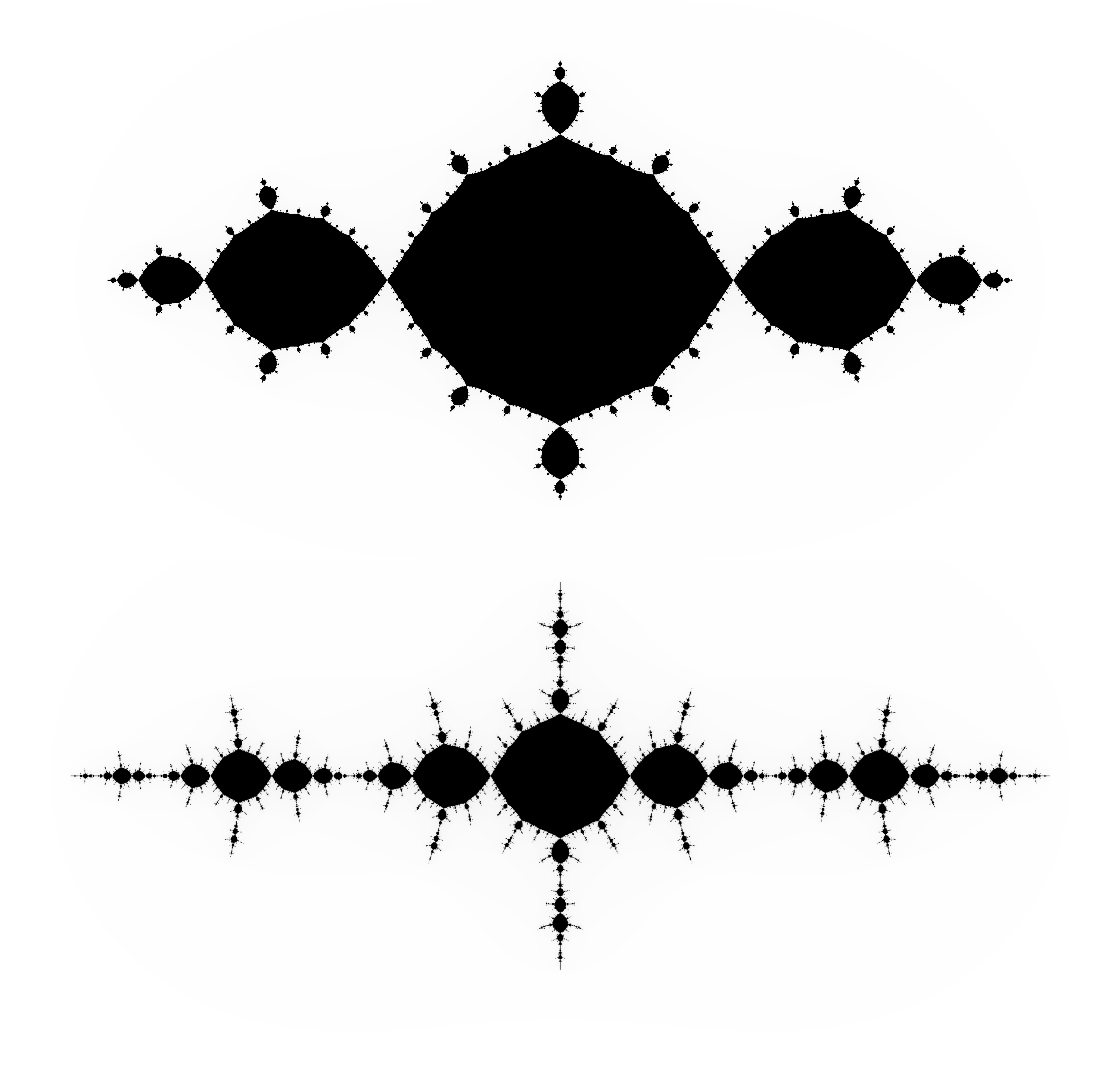
(a)

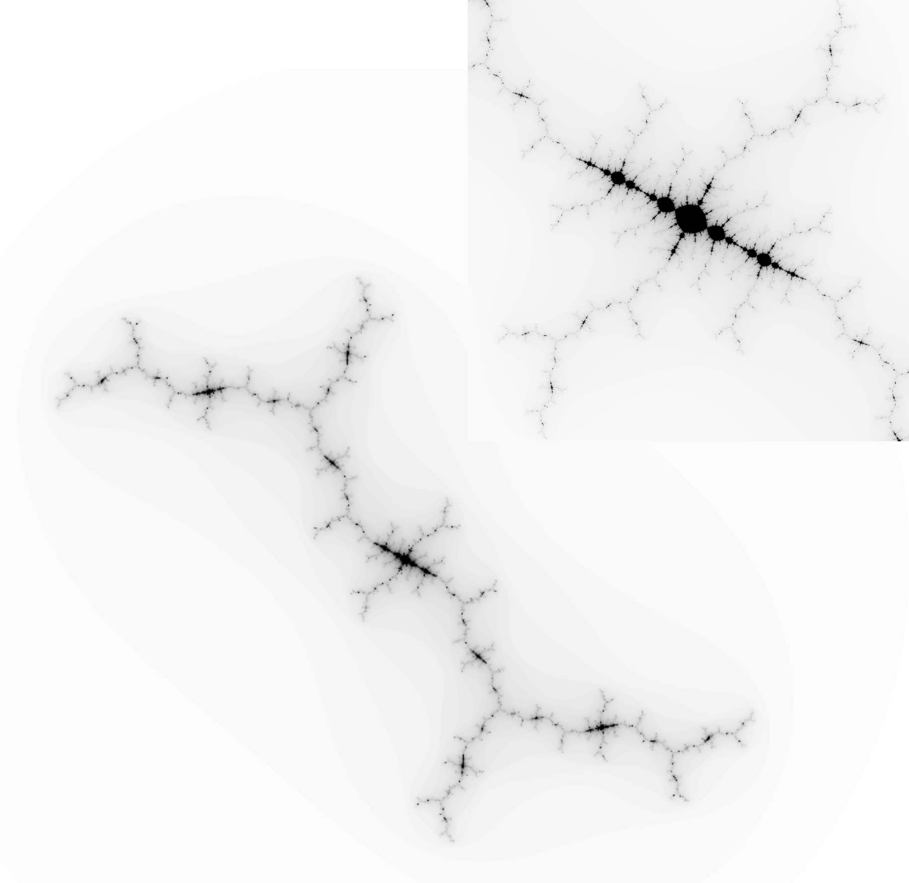
(b)

(c)

(d)

Figure 4.3. (A) Basilica (above, $z^{2}-1$) and the doubled Basilica(below, $z^{2}-1.3107$). (B) Kokopelli tuned with the doubled Basilica ($z^{2}-0.15652+1.03225i$) and the zoomed-in image near 0. (C) Kokopelli tuned with Basilica ($z^{2}-0.16267+1.037123$). (D) Kokopelli ($z^{2}-0.15652+1.03224$).Cores of (B) and (C) are small Basilicas. (C) is the simplicial quotient of (B), and (D) is the simplicial quotient of (C).

Cores of periodic Fatou components

Let $f$ be a post-critically finite polynomial and $\mathcal{K}^{0}$ be the closure of the union of periodic Fatou components. Let $\mathcal{K}^{0}_{1},\mathcal{K}^{0}_{2},\dots,\mathcal{K}^{0}_{l}$ be the connected components of $\mathcal{K}^{0}$. We inductively define $\mathcal{K}^{n}_{i}$ to be the connected component of $f^{-1}(\mathcal{K}^{n-1})$ containing $\mathcal{K}^{n-1}_{i}$ and define $\mathcal{K}^{n}$ to be the union of $\mathcal{K}^{n}_{1},\mathcal{K}^{n}_{2},\dots,\mathcal{K}^{n}_{l}$. It is also inductively obtained that $\mathcal{K}^{n}_{1},\mathcal{K}^{n}_{2},\dots,\mathcal{K}^{n}_{l}$ are pairwise disjoint for any $n\geq 0$.

By construction, for any $i\in\{1,2,\dots,l\},$ $\{\mathcal{K}^{n}_{i}\}_{n\geq 0}$ is an increasing sequence.

Definition 4.17 (Cores).

We use the notations defined above. For any $i\in\{1,2,\dots,l\}$, we call $\mathcal{K}^{\circ}_{i}:=\bigcup_{n}\mathcal{K}^{n}_{i}$ a periodic pre-core and define a periodic core by

$$\mathcal{K}_{i}:=\overline{\mathcal{K}^{\circ}_{i}}.$$

We define the accumulation set of a core $\mathcal{K}_{i}$ by

$$\mathcal{K}^{\omega}_{i}=\mathcal{K}_{i}-\mathcal{K}^{\circ}_{i}.$$

For any periodic core $\mathcal{K}_{i}$ and any $n\geq 1$, we call a connected component $\mathcal{K}^{\circ}$ of $f^{-n}(\mathcal{K}_{i}^{\circ})$ that is not a periodic pre-core a pre-periodic pre-core of $f$. Then we call $\mathcal{K}:=\overline{\mathcal{K}^{\circ}}$ a pre-periodic core and $\mathcal{K}^{\omega}:=\mathcal{K}-\mathcal{K}^{\omega}$ the accumulation set of $\mathcal{K}$.

By a core, we mean a periodic or pre-periodic core.

In the above notations, there are $l$ periodic cores $\mathcal{K}_{1},\mathcal{K}_{2},\dots,\mathcal{K}_{l}$ such that for $i\neq j$, $\mathcal{K}^{\circ}_{i}$ is disjoint from $\mathcal{K}^{\circ}_{j}$ (though $\mathcal{K}_{i}$ may intersect $\mathcal{K}_{j}$). Thus, for every Fatou component $U$, there exists a unique core $\mathcal{K}$ containing $U$.

Let $\mathcal{K}$ be a core. We define the degree of $\mathcal{K}$ by

$$\deg(\mathcal{K}):=1+\sum_{c\in\mathcal{K}^{\circ}}(\deg(f|_{c})-1).$$

One can show that $\mathcal{K}$ is locally connected. Puzzle pieces defined by equipotential curves and eventually periodic external rays shrink, and the intersection of each puzzle piece with $\mathcal{K}$ is connected. We omit details and refer the reader to [OvS09].

Hence there is a Riemann mapping $\phi:\widehat{\mathbb{C}}\setminus\mathbb{D}\to\widehat{\mathbb{C}}\setminus\mathcal{K}$, which continuously extends to the boundary $\phi:\partial\mathbb{D}\to\partial\mathcal{K}$ by the Carathéodory theorem [Mil06, §17]. This domain circle $\partial\mathbb{D}$ is called the ideal boundary of $\mathbb{C}\setminus\mathcal{K}$ and we denote it by $I(\mathbb{C}\setminus\mathcal{K})$.

The map $f:\mathcal{K}\longrightarrow f(\mathcal{K})$ induces a degree $\deg(\mathcal{K})$ covering map

$$f_{*}:I(\mathbb{C}\setminus\mathcal{K})\longrightarrow I(\mathbb{C}\setminus f(\mathcal{K})).$$

We also remark that $\mathcal{K}$ may not be a connected component of $f^{-1}(f(\mathcal{K}))$. This happens if there exists a critical point of $f$ on the accumulation set $\mathcal{K}^{\omega}$. By construction, if $\mathcal{K},\mathcal{K}^{\prime}$ are two distinct cores, then $\mathcal{K}^{\circ}$ and ${\mathcal{K}^{\prime}}^{\circ}$ are disjoint. The following proposition is immediate from the construction.

Proposition 4.18.

Let $f$ be a post-critically finite polynomial. Then two bounded Fatou components $U$ and $V$ are in the same core if and only if there is a finite sequence of bounded Fatou components $U=U_{0},U_{1},\dots,U_{k}=V$ so that $\overline{U}_{i-1}\cap\overline{U}_{i}\neq\emptyset$ for any $i\in\{1,\dots,k\}$.

Construction of simplicial quotients

For a post-critically finite polynomial $f$, the simplicial quotient of $f$ is roughly speaking a post-critically finite polynomial $g$ obtained by replacing each core $\mathcal{K}$ of $f$ with the closure of a new Fatou component $\overline{U}$ of degree $\deg(\mathcal{K})$. A precise construction can be achieved by constructing a desired Hubbard tree in a combinatorial way and then applying Theorem 4.7 as follws.

Let $\mathcal{T}_{f}$ be the Hubbard tree of $f$. Let $v$ be a Fatou vertex of $\mathcal{T}_{f}$. We define a core subtree $\mathcal{T}_{v}$ for $v$ by

$$\mathcal{T}_{v}=\mathcal{T}_{f}\cap\mathcal{K}_{v},$$

where $\mathcal{K}_{v}$ is the core containing the Fatou component $U_{v}$ associated to $v$. Since $\mathcal{T}_{f}$ and $\mathcal{K}_{f}$ are convex respect to regulated arcs, the intersection $\mathcal{T}_{v}$ is indeed a tree. For different Fatou vertices $v$ and $w$, the core subtrees $\mathcal{T}_{v}$ and $\mathcal{T}_{w}$ are same, disjoint, or intersecting at a single point.

Let $\mathcal{T}^{\prime}$ be the closure of a connecomponent $\mathcal{T}_{f}-\mathcal{T}_{v}$. Then $\mathcal{T}^{\prime}$ determines a point on the ideal boundary $x_{\mathcal{T}^{\prime}}\in I(\mathbb{C}\setminus\mathcal{K}_{v})$. Similarly, if $a\in\partial\mathcal{T}_{v}\cap\partial\mathcal{T}_{f}$, then it determines a point on the ideal boundary $x_{a}\in I(\mathbb{C}\setminus\mathcal{K}_{v})$ as well. Let $X_{v}\subseteq I(\mathbb{C}\setminus\mathcal{K}_{v})$ be the collection of all these ideal boundary points, and let $\nu_{v}=\#X_{v}$ be its cardinality.

A tree is called a star if only one vertex, called the center, has valence greater than one. A $k$-star is a star whose center has valence $k$. We construct a new tree by removing $\operatorname{Int}(\mathcal{T}_{v})$ and glue back a $\nu_{v}$-star $\mathcal{T}_{v,new}$ using the ideal boundary information.

We obtain a new tree $\mathcal{T}_{g}$ by performing the above surgery at all Fatou vertices of $\mathcal{T}_{f}$. The map of $f$ on $\mathcal{T}_{f}$ naturally induces a map $g$ on $\mathcal{T}_{g}$. Indeed,

• if $w\notin\bigcup\mathcal{T}_{v,new}$, then $g(w)=f(w)$,

• if $w$ is the center of $\mathcal{T}_{v,new}$, then we define $g(w)$ to be the center of $\mathcal{T}_{f(v),new}$, and

• if $w\in\partial\mathcal{T}_{v,new}$, then $g(w)\in\partial\mathcal{T}_{f(v),new}$ is determined by the induced map between the ideal boundaries $f_{*}:I(\mathbb{C}\setminus\mathcal{K}_{v})\longrightarrow I(\mathbb{C}\setminus\mathcal{K}_{f(v)})$.

The map $g$ is then extended on the edges $[w,w^{\prime}]$ so that

$$g([w,w^{\prime}])=[g(w),g(w^{\prime})].$$

Inherited from the local degree on $\mathcal{T}_{f}$, we remark that the local degrees of a vertex of $\mathcal{T}_{g}$ can be naturally defined, and a vertex is called critical if it has local degree $\geq 2$. By removing some endpoints and the corresponding edges of $\mathcal{T}_{g}$ if necessary, we may assume $\mathcal{T}_{g}$ is the convex hull of critical and post-critical points. The ideal boundary also gives the angle structure on the new tree $\mathcal{T}_{g}$. More precisely, angles at the center of stars are defined from the ideal boundaries and angels at the other vertices are induced from angles of $\mathcal{T}_{f}$. Therefore, $\mathcal{T}_{g}$ is an abstract Hubbard tree. The marking for $\mathcal{T}_{f}$ induces a marking for $\mathcal{T}_{g}$. Thus, by Theorem 4.8, there exists a unique post-critically finite polynomial $g\in\mathcal{P}_{d}$ realizing this abstract Hubbard tree $\mathcal{T}_{g}$.

Definition 4.19 (Simplicial quotients).

Let $f$ be a post-critically finite polynomial with Hubbard tree $\mathcal{T}_{f}$. Let $\mathcal{T}_{g}$ be the marked abstract Hubbard tree constructed as above. We call the corresponding post-critically finite polynomial $g\in\mathcal{P}_{d}$ the simplicial quotient of $f$.

It is clear from the construction that $f$ is a simplicial tuning of $g$. We have the following bijection

$$\{\mathrm{cores\leavevmode\nobreak\ of\leavevmode\nobreak\ }f\}\longleftrightarrow\{\mathrm{bounded\leavevmode\nobreak\ Fatou\leavevmode\nobreak\ components\leavevmode\nobreak\ of\leavevmode\nobreak\ }g\}.$$

This induces a natural surjection between the sets of critical and post-critical points

$$q:\operatorname{\mathrm{Crit}}(f)\cup P_{f}\rightarrow\operatorname{\mathrm{Crit}}(g)\cup P_{g}$$

which sends all the critical or post-critical points in $\mathcal{K}^{\circ}$ for each core $\mathcal{K}$ of $f$ to the center of the corresponding Fatou component of $g$. The following lemma is immediate from these correspondences.

Lemma 4.20.

Let $g$ be the simplicial quotient of a post-critically finite polynomial $f$ and $q:\operatorname{\mathrm{Crit}}(f)\cup P_{f}\rightarrow\operatorname{\mathrm{Crit}}(g)\cup P_{g}$ be the induced surjection on the sets of critical and post-critical points. If $x\in\operatorname{\mathcal{J}}_{g}\cap(\operatorname{\mathrm{Crit}}(g)\cup P_{g})$, then every point in $q^{-1}(x)$ is in the accumulation set of a core of $f$.

By considering $f$ as a simplicial tuning of $g$, we can use the defintions of internal and external edges in Definition 4.11. Internal edges of simplicial quotients are periodic or preperiodic.

Lemma 4.21 (Depths of internal edges of $g$).

Let $g$ be the simplicial quotient of a post-critically finite polynomial $f$. Then the following are equivalent:

• an edge $e$ of $\mathcal{T}_{g}$ is an internal edge.

• $e$ is periodic or preperiodic.

• $\operatorname{\mathrm{depth}}(e)=0$.

Proof.

Every internal edge is an edge of a star, so it is periodic or preperiodic. By definition every periodic or preperiodic edge has depth 0. Suppoe $e$ is an external edge. The endpoints of $e$ are Julia points. If $e$ has depth 0, then $e$ consists of preimages of periodic edges. It follows that $e$ has to be contained in a core of $f$, which contradicts to the assumption that $e$ is an external edge. ∎

The same proof as Lemma 4.13 gives:

Lemma 4.22 (Depths of internal edges of $f$).

Let $f$ be a post-critically finite polynomial and $\mathcal{T}_{f}$ be its Hubbard tree. Let $v$ be a Fatou vertex in $\mathcal{T}_{f}$. Let $\mathcal{T}_{v}$ be the core subtree of $\mathcal{T}_{f}$ whose core is $\mathcal{K}$, and let $e$ be an edge of $\mathcal{T}_{v}$. If any endpoint of $e$ is not an boundary point of $\mathcal{T}_{v}$, then $\operatorname{\mathrm{depth}}(e)=0$. If $e$ has an endpoint $w$ that is a boundary point of $\mathcal{T}_{v}$, then

• $\operatorname{\mathrm{depth}}(e)=0$ if and only if $w\in\mathcal{K}^{\circ}$, and

• $\operatorname{\mathrm{depth}}(e)=1$ if and only if $w\in\mathcal{K}^{\omega}$.

The following proposition follows immediately from definitions.

Proposition 4.23.

Let $f(z)\neq z^{d}$ be a post-critically finite polynomial. Then the following are equivalent:

1. $\mathcal{T}_{f}$ is simplicial.

2. $\mathscr{C}_{gr}(f)=1$.

3. $f$ has only one core.

4. The simplicial quotient of $f$ is $z^{d}$.

Non-triviality of simplicial quotient

A core $\mathcal{K}$ of a post-critically finite polynomial $f$ is said to be trivial if it contains only one Fatou component.

Lemma 4.24.

Let $f\in\mathcal{P}_{d}$ be a post-critically finite polynomial with core entropy zero. If $f(z)\neq z^{d}$, then it has at least one non-trivial core.

Before proving Lemma 4.24, let us discuss its consequences first. Let $f\in\mathcal{P}_{d}$ be a post-critically finite polynomial, and let

• $k_{f}$ be the number periodic bounded Fatou components, and

• $m_{f}$ be the number of critical points in periodic bounded Fatou components counted with multiplicities.

Note that $m_{f}\leq d-1$.

Lemma 4.25.

Let $f(z)\neq z^{d}\in\mathcal{P}_{d}$ be a post-critically finite polynomial with core entropy zero. Let $g$ be the simplicial quotient of $f$. Then either

• $k_{g}<k_{f}$, or

• $m_{g}>m_{f}$.

Proof.

Recall that Fatou components of $f$ which can be joined by finite sequences of adjacent Fatou components are merged to one Fatou component of $g$ (Proposition 4.18). Hence $k_{g}\leq k_{f}$ and $m_{g}\geq m_{f}$ are clear from the construction. Suppose $k_{g}=k_{f}$. We will show $m_{g}>m_{f}$.

By Lemma 4.24, there exists a non-trivial periodic core $\mathcal{K}$ of $f$. Without loss of generality, we assume that $\mathcal{K}$ is fixed and there exists a fixed Fatou component $U$ in $\mathcal{K}$.

Since $k_{g}=k_{f}$, $\overline{U}$ does not intersect with the closures of other periodic Fatou components. Recall the construction of cores for periodic Fatou components. Suppose for contradiction that $\partial U$ does not contain any critical points of $f$. The connected component $\mathcal{K}^{1}_{U}$ of $f^{-1}(\overline{U})$ that contains $U$ is $\overline{U}$. Thus, by induction $\mathcal{K}^{n}_{U}=\overline{U}$, so $\mathcal{K}=\overline{\bigcup_{n}\mathcal{K}^{n}_{U}}=\overline{U}$, which contradicts to that $\mathcal{K}$ is non-trivial. Therefore, $\mathcal{K}$ contains at least one additional critical point of $f$.

By the construction of simplicial quotients, the corresponding fixed Fatou component of $g$ has a critical fixed point whose multiplicity is strictly greater than the multiplicity of the center of $U$. Since the other periodic Fatou components of $g$ contain at least the same number of critical points of $g$ as the corresponding periodic Fatou components of $f$ counted with multiplicities, we have $m_{g}>m_{f}$. ∎

Theorem 4.16 now follows from Lemma 4.25.

Proof of Theorem 4.16.

Let $f_{0}=f$, and let $f_{1}$ be the simplicial quotient of $f_{0}$. It is easy to verify that the core entropy of the simplicial quotient $f_{1}$ is still zero. Thus, if $f_{1}(z)\neq z^{d}$, the above argument also applies to $f_{1}$. Since $k_{f}\geq 0$ and $m_{f}\leq d-1$ are both integers, the process must terminate in finite steps. Theorem 4.16 now follows. ∎

We now prove Lemma 4.24.

Proof of Lemma 4.24.

Suppose for contradiction that all periodic cores are trivial. For each Fatou vertex $v$, let $\mathcal{T}_{v}\subseteq\mathcal{T}_{f}$ be the core subtree. Since every periodic core is trivial, $\mathcal{T}_{v}$’s are stars. We consider a quotient map

$$\Phi:\mathcal{T}_{f}\longrightarrow\widetilde{\mathcal{T}_{f}}=\mathcal{T}_{f}/\sim,$$

where two points are identified if they are in the same core subtree $\mathcal{T}_{v}$. We remark that $\widetilde{\mathcal{T}_{f}}$ may not be a Hubbard tree.

The dynamics of $f:\mathcal{T}_{f}\longrightarrow\mathcal{T}_{f}$ induces a map $\tilde{f}:\widetilde{\mathcal{T}_{f}}\longrightarrow\widetilde{\mathcal{T}_{f}}$. Since $h(f)=0$, $h(\tilde{f})=0$. Thus, there exists a periodic edge $\widetilde{E}\subseteq\widetilde{\mathcal{T}_{f}}$, i.e., $\tilde{f}^{k}:\widetilde{E}\longrightarrow\widetilde{E}$ is a homeomorphism, where $k$ is the period of $\widetilde{E}$. Without loss of generality, we assume $\widetilde{E}=[\tilde{v},\tilde{w}]$ is fixed, and the homeomorphism is orientation preserving.

Let $E^{\prime}=\Phi^{-1}(\widetilde{E})$. Since $\tilde{f}(\widetilde{E})=\widetilde{E}$, we have $f(E^{\prime})\subseteq E^{\prime}$. Let $E$ be an edge in $\overline{E^{\prime}-\bigcup_{v}\mathcal{T}_{v}}$, which exists becasue $T_{v}$’s are disjoint. The edge $E$ is an exterior edge of $\mathcal{T}_{f}$. Denote the endpoints of $E$ by $a_{1}$ and $a_{2}$.

We show that $f:E\longrightarrow E$ is a homeomorphism. It suffices to prove $f(a_{i})=a_{i}$ for $i\in\{1,2\}$. If $a_{i}\notin\mathcal{T}_{v}$ for any Fatou vertex $v$, then $\Phi^{-1}(\Phi(a_{i}))=\{a_{i}\}$. Then it follow from $\Phi:\widetilde{E}\longrightarrow\widetilde{E}$ being homeomorphic that $f(a_{i})=a_{i}$. If $a_{i}\in\mathcal{T}_{v}$ for some Fatou vertex, there is a fixed Fatou component $U_{v}$ with $a_{i}\in\partial U$. Suppose for contradiction that $f(a_{i})\neq a_{i}$. Since $f(E)\subseteq E^{\prime}$, this forces $a_{i}$ to be a critical point. This is a contradiction to the core of $U$ being trivial. Hence $f(a_{i})=a_{i}$ and $f:E\to E$ is a homeomorphism.

Since $f:\mathcal{T}_{f}\longrightarrow\mathcal{T}_{f}$ is expanding (Definition 4.3), $E$ must contain a fixed Fatou point. This is contradiction as $E$ is an exterior edge. ∎

4.4. Bounding the combinatorial complexity

Proof of Theorem 4.1.

Suppose $f$ has core entropy zero. Then by Theorem 4.16, there exists a finite sequence $f_{0}=f,f_{1},...,f_{k}(z)=z^{d}$ such that $f_{i+1}$ is the simplicial quotient of $f_{i}$. Since $f_{i}$ is a simplicial tuning of $f_{i+1}$, $f$ is obtained from $z^{d}$ by a finite sequence of simplicial tunings. The reverse direction follows from Corollary 4.15. ∎

To prove Theorem 4.2, we need a bound of $\mathscr{C}_{c}(f)$ on the other direction. To achieve this, we prove the following lemma (cf. Lemma 4.14).

Lemma 4.26.

Let $f\in\mathcal{P}_{d}$ be a post-critically finite polynomial with core entropy zero, with $f(z)\neq z^{d}$. Let $g$ be the simplicial quotient of $f$. Then

$$\mathscr{C}_{gr}(f)=\mathscr{C}_{gr}(g)+1.$$

Proof.

By Lemma 4.14, it suffices to show $\mathscr{C}_{gr}(f)\geq\mathscr{C}_{gr}(g)+1$.

Let $\mathcal{T}_{f}$ and $\mathcal{T}_{g}$ be the Hubbard trees for $f$ and $g$. Note that $f$ is a simplicial tuning of $g$ (see §4.2). The Hubbard tree $\mathcal{T}_{f}$ is constructed from $\mathcal{T}_{g}$ by removing $\mathcal{T}_{v}$ and gluing back $\mathcal{T}_{v,f}$, where $v$ is a branch Fatou point, or a critical or post-critical Fatou point. Here we use the notation $\mathcal{T}_{v,f}$ instead of $\mathcal{T}_{v,new}$, which was used in §4.2, to emphasize the dependence on $f$.

We define the vertex set $\mathcal{V}_{g}$ as the smallest forward invariant set of $\mathcal{T}_{g}$ containing the critical points, branch points, and $\partial\mathcal{T}_{v}$. Let $\mathcal{G}_{f}$ and $\mathcal{G}_{g}$ be the corresponding directed graphs.

Let $a\in\mathcal{G}_{g}$ be a vertex with maximal depth so that $\mathscr{C}_{gr}(g)=1+\operatorname{\mathrm{depth}}(a)$. Let $m=\operatorname{\mathrm{depth}}(a)$. Then by Lemma 2.12, we have a maximal sequence

$$a=a_{0}\geq a_{1}\geq...\geq a_{m}$$

where $a_{i}$’s are in disjoint simple cycles $\mathcal{C}_{i}$.

Consider the case $\mathscr{C}_{gr}(g)\leq 1$. We use properties polynomials with simplicial Hubbard trees (see Proposition 4.23). If $\mathscr{C}_{gr}(g)=0$, then $g=z^{d}$. Then the Hubbard tree $\mathcal{T}_{f}$ of $f$ is simplicial so that $\mathscr{C}_{gr}(f)=1$. If $\mathscr{C}_{gr}(g)=1$, then $\mathcal{T}_{g}$ is simplicial. If $\mathscr{C}_{gr}(f)=1$ as well, then $\mathcal{T}_{f}$ is also simplicial. Then $g=z^{d}$ because $g$ is the simplicial quotient of $f$, which contradicts to $\mathscr{C}_{gr}(g)=1$. Hence we may assume $m=\mathscr{C}_{gr}(g)-1\geq 1$.

Let $E_{i}$ be the corresponding edge of $\mathcal{T}_{g}$ for $a_{i}$. Let $l_{i}$ be the length of the cycle $\mathcal{C}_{i}$. By the maximality of the sequence $(a_{i})$, the map

$$g^{l_{m}}:E_{m}\longrightarrow E_{m}$$

is a homeomorphism. It follows from Lemma 4.21 that $E_{m}$ is an internal edge and $E_{i}$ is an external edge for all $i<m$.

Since external edges of $\mathcal{T}_{f}$ and $\mathcal{T}_{g}$ are in bijective correspondence, we have an external edge $\widetilde{E_{i}}$ of $\mathcal{T}_{f}$ that corresponds to the external edge $E_{i}$ of $\mathcal{T}_{g}$ for $i<m$. Let $\tilde{a}_{0}\geq\tilde{a}_{1}\geq...\geq\tilde{a}_{m-1}$ be the vertices in $\mathcal{G}_{f}$ corresponding to $\widetilde{E_{i}}$. Note that $\tilde{a}_{i}$ are in disjoint simple cycles.

It suffices to show that $\tilde{a}_{m-1}$ has depth at least 2. To prove this, we denote the internal edge $E_{m}$ by $E_{m}=[x,y]$, where $x$ is the center of a periodic Fatou component $U$ and $y\in\partial U_{v}$. By the definition of simplicial quotient, the boundary point $y$ corresponds to a point $\tilde{y}\in\partial\mathcal{T}_{v,f}\subset\mathcal{T}_{f}$.

Claim: There exists a point $y^{\prime}\in\operatorname{Int}(E_{m-1})$ with $g^{k}(y^{\prime})=y$ for some $k$. Therefore, either

• $y$ is in the forward orbit of a critical point of $g$, or

• there exists another edge $E_{m}^{\prime}$ with $y\in\partial E_{m}^{\prime}$ so that $E_{m}^{\prime}\subseteq g^{k}(E_{m-1})$.

Proof of the claim.

Since $a_{m-1}\geq a_{m}$ and $a_{m-1}$ and $a_{m}$ are in different cycles, we have

$$\limsup_{n\to\infty}\#\{\mathrm{paths\leavevmode\nobreak\ from\leavevmode\nobreak\ }a_{m-1}\mathrm{\leavevmode\nobreak\ to\leavevmode\nobreak\ }a_{m}\}=\infty.$$

Hence there exists $k>0$ so that at least three small segments of $E_{m-1}$ are homeomorphically mapped onto $E_{m}$ by $f^{k}$. Then we have $y^{\prime}\in\operatorname{Int}(E_{m-1})$ with $f^{k}(y^{\prime})=y$.

The cases (1) and (2) are determined according to whether $f^{k}$ folds $E_{m-1}$ at $y^{\prime}$. ∎

We now show $\operatorname{\mathrm{depth}}(\tilde{a}_{m-1})\geq 2$ for each of the cases (1) and (2).

Case (1): Suppose that $y$ is in the forward orbit of a critical point of $g$. By Lemma 4.20, $\tilde{y}$ is in the accumulation set of the core $\mathcal{K}_{v}$. Thus, $\tilde{y}$ is an endpoint of $\mathcal{T}_{v,f}$. Hence, there is a unique edge $\widetilde{E_{m}}$ of $\mathcal{T}_{v,f}$ that has $\tilde{y}$ as an endpoint so that $\widetilde{E_{m}}\subseteq f^{n}(\widetilde{E_{m-1}})$ for some $n>0$. Let $\tilde{a}_{m}$ be the vertex of $\mathcal{G}_{f}$ corresponding to $\widetilde{E_{m}}$. It follows from Lemma 4.22 that $\operatorname{\mathrm{depth}}(\tilde{a}_{m})=1$. Since $\tilde{a}_{m-1}\geq\tilde{a}_{m}$ and they are in disjoint simple cycles, $\operatorname{\mathrm{depth}}(\tilde{a}_{m-1})\geq 2$.

Case (2): Suppose that there exists another edge $E_{m}^{\prime}$ with $y\in\partial E_{m}^{\prime}$ so that $E_{m}^{\prime}\subseteq g^{k}(E_{m-1})$. By the maximality assumption, $\operatorname{\mathrm{depth}}(E_{m}^{\prime})=0$. Thus, $E_{m}^{\prime}$ is also an internal edge by Lemma 4.21. Hence, $E_{m}^{\prime}\subseteq\mathcal{T}_{v^{\prime}}$ for some $v^{\prime}$. By Proposition 4.18, $\tilde{y}$ is in the accumulation set of either $\mathcal{K}_{v}$ or $\mathcal{K}_{v^{\prime}}$. Without loss of generality, we may assume that $\tilde{y}$ is in the accumulation set of the core $\mathcal{K}_{v}$. Let $\widetilde{E_{m}}$ be the edge of $\mathcal{T}_{v,f}$ having $\tilde{y}$ as an endpoint and let $\tilde{a}_{m}$ be the corresponding vertex in $\mathcal{G}_{f}$. By Lemma 4.22, $\tilde{a}_{m}$ has depth $1$. Since $\tilde{a}_{m-1}\geq\tilde{a}_{m}$ and they are in disjoint simple cycles, we have $\operatorname{\mathrm{depth}}(\tilde{a}_{m-1})\geq 2$. ∎

Theorem 4.2 now follows immediately.

Proof of Theorem 4.2.

By Corollary 4.15, $\mathscr{C}_{c}(f)\geq\mathscr{C}_{gr}(f)$.

On the other hand, let $f_{0}=f,f_{1},...,f_{k}(z)=z^{d}$ with $f_{i+1}$ is the simplicial quotient of $f_{i}$. By Lemma 4.26, $\mathscr{C}_{gr}(f)=k$. Thus $\mathscr{C}_{c}(f)\leq\mathscr{C}_{gr}(f)$. ∎

Remark 4.27.

We remark that from the proof, the sequence of simplicial quotients $f_{0}=f,f_{1},...,f_{k}(z)=z^{d}$ with $f_{i+1}$ is the simplicial quotient of $f_{i}$ gives the minimal number of simplicial tunings to obtain $f$ from $z^{d}$.

5. Bifurcation from simplicial tuning

In this section, we use the theory developed in [Luo21, Luo22] to study the relations between bifurcations and simplicial tunings. The main result we will prove in this section is the following theorem.

Theorem 5.1.

Let $g\in\mathcal{P}_{d}$ be a post-critically finite polynomial. Let $f\in\mathcal{P}_{d}$ be a simplicial tuning of $g$. Then $\mathcal{H}_{g}$ bifurcates to $\mathcal{H}_{f}$.

The idea is to construct a sequence $g_{n}$ of quasi post-critically finite degenerations in $\mathcal{H}_{g}$ that converges to a root $g_{\infty}$ of $\mathcal{H}_{f}$, which will be defined in this section. These quasi post-critically finite degenerations are combinatorially parameterized by quasi invariant forests and allow us to change the dynamics on the bounded Fatou component of $g$. As a corollary, we have:

Corollary 5.2.

Let $f\in\mathcal{P}_{d}$ be obtained by a finite sequence of simplicial tunings from $z^{d}$. Then $f\in\mathscr{M}_{d}$.

Recall that the bifurcation complexity $\mathscr{C}_{b}(f)$ is the smallest number of relative hyperbolic components one needs to bifurcate to arrive at $\mathcal{H}_{f}$ from $\mathcal{H}_{d}$, and the combinatorial complexity $\mathscr{C}_{c}(f)$ is the smallest number of simplicial tunings needed to get $f$. Here we allow $\mathscr{C}_{b}(f)$ and $\mathscr{C}_{c}(f)$ to be $+\infty$ if there are no finite chains of bifurcation or simplicial tunings. There is an inequality between these two complexities.

Theorem 5.3.

Let $f\in\mathcal{P}_{d}$ be a post-critically finite polynomial. Then

$$\mathscr{C}_{b}(f)\leq\mathscr{C}_{c}(f).$$

Moreover, the bound is sharp, i.e., there exists a degree $d$ post-critically finite polynomial $f$ with $\mathscr{C}_{c}(f)=\mathscr{C}_{b}(f)$.

Quasi post-critically finite degeneration

Let us briefly summarize the theory of quasi post-critically finite degeneration. We refer the reader to [Luo21, Luo22] for more details.

Let $\mathcal{S}=(|\mathcal{S}|,\Phi,\delta)$ be a mapping scheme. Consider the Blaschke model space $\operatorname{\mathcal{B}}^{\mathcal{S}}$, which is defined in Definition 3.6. We first define an extended metric, a metric allowing $\infty$ distances, $d_{\mathcal{S}}$ on $|\mathcal{S}|\times\mathbb{D}$ by

• $d_{\mathcal{S}}(x,y)=\infty$ if $x\in s\times\mathbb{D}$ and $y\in t\times\mathbb{D}$ with $s\neq t$, and

• $d_{\mathcal{S}}(x,y)=d_{s\times\mathbb{D}}(x,y)$ if $x,y\in s\times\mathbb{D}$,

where $d_{s\times\mathbb{D}}$ is the hyperbolic metric on the unit disk.

We are interested in a particular degeneration in $\operatorname{\mathcal{B}}^{\mathcal{S}}$, called quasi post-critically finite degeneration.

Definition 5.4 (Quasi post-critically finite degeneration).

Let $\mathcal{S}$ be a mapping scheme of degree $d$ and $\operatorname{\mathcal{B}}^{\mathcal{S}}$ be the corresponding Blaschke model space. Let $\{\mathcal{F}_{n}\}$ be a sequence in $\operatorname{\mathcal{B}}^{\mathcal{S}}$. For $K>0$, $\mathcal{F}_{n}$ is said to be $K$-quasi post-critically finite if we can label the critical points by $c_{1,n},...,c_{2d-2,n}$, and for any sequence $\{c_{i,n}\}_{n}$ of critical points, there exist $l_{i}$ and $q_{i}$, called quasi pre-periods and quasi periods respectively, such that for any $n>0$ we have

$$d_{\mathcal{S}}(\mathcal{F}_{n}^{l_{i}}(c_{i,n}),\mathcal{F}_{n}^{l_{i}+q_{i}}(c_{i,n}))\leq K.$$

We say $\{\mathcal{F}_{n}\}$ is quasi post-critically finite if it is $K$-quasi post-critically finite for some $K>0$.

Quasi invariant forests

A ribbon structure on a finite tree is a choice of planar embedding up to isotopy. A ribbon structure can also be defined as the assignment of a cyclic ordering of the edges incident to each vertex. A ribbon finite tree is a finite tree with a ribbon structure, and an isomorphism between ribbon finite trees is an isomorphism between finite trees that preserves the ribbon structures. A marked finite tree $(\mathcal{T},\mathcal{P})$ is a finite tree with a subset $\mathcal{P}\subseteq\mathcal{V}$ of the vertex set $\mathcal{V}$ for $\mathcal{T}$.

In [Luo22, §3], for any quasi post-critically finite sequence $\{\mathcal{F}_{n}\in\operatorname{\mathcal{B}}^{\mathcal{S}}\}$, a sequence of marked ribbon forests

$$(\mathcal{T}_{n},\mathcal{P}_{n}):=\bigcup_{s\in|\mathcal{S}|}(\mathcal{T}_{s,n},\mathcal{P}_{s,n})$$

is constructed, where each $\mathcal{T}_{s,n}\subseteq s\times\mathbb{D}$ is a finite ribbon tree. We call $(\mathcal{T}_{n},\mathcal{P}_{n})$’s the quasi-invariant forests for the sequence $\{\mathcal{F}_{n}\}$. They captures all interesting dynamical features of the sequence $\{\mathcal{F}_{n}\}$, which can be modeled by simplicial maps, as described in the following theorem.

Theorem 5.5 ([Luo22] Theorem 3.2).

Let $\mathcal{S}=(|\mathcal{S}|,\Phi,\delta)$ be a mapping scheme and $\{\mathcal{F}_{n}\}$ be a quasi post-critically finite sequence in $\operatorname{\mathcal{B}}^{\mathcal{S}}$. After passing to a subsequence, there exist a constant $K>0$, a marked ribbon forest $(\mathcal{T},\mathcal{P})=\bigcup_{s\in|\mathcal{S}|}(\mathcal{T}_{s},\mathcal{P}_{s})$ with vertex set $\mathcal{V}=\bigcup_{s\in|\mathcal{S}|}\mathcal{V}_{s}$, where $(\mathcal{T}_{s},\mathcal{P}_{s})$ is a marked ribbon finite tree, a simplicial map

$$F=\bigcup_{s\in|\mathcal{S}|}F_{s}:(\mathcal{T},\mathcal{P})=\bigcup_{s\in|\mathcal{S}|}(\mathcal{T}_{s},\mathcal{P}_{s})\longrightarrow(\mathcal{T},\mathcal{P})$$

with

$$F_{s}:(\mathcal{T}_{s},\mathcal{P}_{s})\longrightarrow(\mathcal{T}_{\Phi(s)},\mathcal{P}_{\Phi(s)}),$$

and a sequence of isomorphisms

$$\phi_{n}:(\mathcal{T},\mathcal{P})\longrightarrow(\mathcal{T}_{n},\mathcal{P}_{n})$$

where $(\mathcal{T}_{n},\mathcal{P}_{n})$’s are the quasi-invariant forests for $\{\mathcal{F}_{n}\}$ such that the following properties hold.

• (Degenerating vertices.) If $v_{1}\neq v_{2}\in\mathcal{V}$, then

  $$d_{\mathcal{S}}(\phi_{n}(v_{1}),\phi_{n}(v_{2}))\to\infty.$$

• (Geodesic edges.) If $E=[v_{1},v_{2}]\subseteq\mathcal{T}$ is an edge, then the corresponding edge $\phi_{n}(E)\subseteq\mathcal{T}_{n}$ is a hyperbolic geodesic segment connecting $\phi_{n}(v_{1})$ and $\phi_{n}(v_{2})$.

• (Critically approximating.) Any critical points of $\mathcal{F}_{n}$ are within $K$ distance from the vertex set $\mathcal{V}_{n}:=\phi_{n}(\mathcal{V})$ of $\mathcal{T}_{n}$.

• (Quasi-invariance on vertices.) If $v\in\mathcal{V}$, then

  $$d_{\mathcal{S}}(\mathcal{F}_{n}(\phi_{n}(v)),\phi_{n}(F(v)))\leq K\text{ for all }n.$$

• (Quasi-invariance on edges.) If $E\subseteq\mathcal{T}$ is an edge and $x_{n}\in\phi_{n}(E)$, then there exists $y_{n}\in\phi_{n}(F(E))$ so that

  $$d_{\mathcal{S}}(\mathcal{F}_{n}(x_{n}),y_{n})\leq K\text{ for all }n.$$

  If $E$ is a periodic edge of period $q$, then

  $$d_{\mathcal{S}}(\mathcal{F}_{n}^{q}(x_{n}),x_{n})\leq K\text{ for all }n.$$

Remark 5.6.

By the construction in [Luo22, §3], if $s\in|\mathcal{S}|$ is periodic under $\Phi$, then $\mathcal{P}_{s}$ consists of a single point $p_{s}$, and $\phi_{n}(p_{s})\in\{s\}\times\mathbb{D}$ is the unique attracting periodic point in $\{s\}\times\mathbb{D}$ for $\mathcal{F}_{n}$.

Rescaling limits

Let $v\in\mathcal{V}_{s}\subseteq\mathcal{V}$. We define a normalization at $v$ or a coordinate at $v$ as a sequence $\{M_{v,n}\in\operatorname{Isom}(\mathbb{H}^{2})\}_{n}$ so that

$$\phi_{n}(v)=(s,M_{v,n}(0)).$$

Note that different choices for the sequence $\{M_{v,n}\}_{n}$ are differed by pre-composing with rotations that fix $0$, which form a compact group. We define a map

$$\hat{M}_{v,n}:\mathbb{D} \longrightarrow\{s\}\times\mathbb{D}$$

$$z \mapsto(s,M_{v,n}(z)).$$

Let us fix such a normalization $\{M_{v,n}\}_{n}$ for each vertex $v\in\mathcal{V}$. To distinguish normalizations at different vertices, we use $\mathbb{D}_{v}$ to denote the disk associated to the normalization at $v$. By the quasi-invariance on vertices in Theorem 5.5, we have

$$d_{\mathcal{S}}(\mathcal{F}_{n}(\phi_{n}(v)),\phi_{n}(F(v)))\leq K$$

for some constant $K$. Thus, $d_{\mathbb{D}}(\hat{M}_{F(v),n}^{-1}\circ\mathcal{F}_{n}\circ\hat{M}_{v,n}(0),0)\leq K$. Therefore, by [Luo21, Proposition 2.3], after possibly passing to a subsequence, the sequence of proper maps

$$\hat{M}_{F(v),n}^{-1}\circ\mathcal{F}_{n}\circ\hat{M}_{v,n}:\mathbb{D}_{v}\longrightarrow\mathbb{D}_{F(v)}$$

converges compactly to a proper holomorphic map

$$\mathcal{R}_{v}=\mathcal{R}_{v\to F(v)}:\mathbb{D}_{v}\longrightarrow\mathbb{D}_{F(v)}.$$

We call this map $\mathcal{R}_{v}$ the rescaling limit of $\mathcal{F}_{n}$ at $v$ and denote its degree by $\delta(v)$. We remark there are exactly $\delta(v)-1$ critical points of $\mathcal{F}_{n}$ counted with multiplicity that stay within a uniform $d_{\mathcal{S}}$-distance from $\phi_{n}(v)$. By critically approximating property in Theorem 5.5, we have for any $s\in|\mathcal{S}|$,

$$\delta(s)=1+\sum_{v\in\mathcal{V}_{s}}(\delta(v)-1).$$

A vertex $v\in\mathcal{V}$ is critical if $\delta(v)\geq 2$. A vertex is called a Fatou point if it is eventually mapped to a critical periodic orbit, and is called a Julia point otherwise.

Angled forest map

To give a combinatorial description of quasi-invariant forests, we introduce the notion of angled forest here. This is a straightforward generalization of angled tree maps in [Luo21, §3], to which we refer the readers for more details and comparisons with abstract Hubbard trees.

Let $m_{d}:\mathbb{S}^{1}\longrightarrow\mathbb{S}^{1}$ denote the multiplication by $d$ map where $\mathbb{S}^{1}$ is identified with $\mathbb{R}/\mathbb{Z}$. By our convention, $m_{1}$ is the identity map. For $d\geq 2$, $m_{d}$ gives a topological model of the dynamics on the Julia set of a degree $d$ hyperbolic and a doubly parabolic Blaschke product (see §3.1 for definitions).

To set up a framework that also works for singly parabolic or boundary-hyperbolic Blaschke products uniformly, we consider an extended circle $\mathbb{S}^{1}_{d}$, which is naturally regarded as cyclically ordered set (see [McM09b, §2]). As a set, $\mathbb{S}^{1}_{d}$ is constructed from $\mathbb{S}^{1}$ by adding (formal symbols) $x^{-},x^{+}$ for any point $x$ in the backward orbit of $0$ under $m_{d}$ for $d\geq 2$. The cyclic ordering on $\mathbb{S}^{1}_{d}$ is defined so that $x^{-}$ (or $x^{+}$) is regarded as a point infinitesimally smaller than $x$ (or bigger than $x$ respectively) in the standard identification of $\mathbb{S}^{1}=\mathbb{R}/\mathbb{Z}$. Note that $\mathbb{S}^{1}$ naturally embeds into $\mathbb{S}^{1}_{d}$. We call a point in the image of this embedding a regular point. We use the convention that $\mathbb{S}^{1}_{1}=\mathbb{S}^{1}$.

Given any integer $k\geq 1$, the map $m_{k}$ naturally extends to $m_{k}:\mathbb{S}^{1}_{d}\longrightarrow\mathbb{S}^{1}_{d}$ by setting $m_{k}(x^{\pm})=m_{k}(x)^{\pm}$. This is well-defined because if $x$ is in the backward orbit of $0$ under $m_{d}$, $m_{k}(x)$ is also in the backward orbit of $0$ under $m_{d}$.

If $f$ is a degree $d$ boundary-hyperbolic Blaschke product, i.e., $f$ has an attracting fixed point $a$ on the circle, the Julia set $J$ of $f$ is a Cantor set on $\mathbb{S}^{1}$. The complement $\mathbb{S}^{1}-J$ consists of countably many intervals, which are all eventually mapped to the unique interval $I\subseteq\mathbb{S}^{1}$ that contains the attracting fixed point $a$. The boundary $\partial I$ consists of two repelling fixed points of $f$. Let $\mathcal{O}(a)$ be the backward orbit of the attracting fixed point $a$. Then there exists bijective map $\eta_{f}:\mathbb{S}^{1}_{d}\longrightarrow J(f)\cup\mathcal{O}(a)$ which preserves the cyclic ordering so that $f\circ\eta_{f}=\eta_{f}\circ m_{d}$. Note that $\eta_{f}(0)=a$, and $\eta_{f}(0^{\pm})=\partial I$ (see Figure 5.1).

Figure 5.1. An illustration of the conjugacy $\eta_{f}$ for a degree $3$ boundary-hyperbolic Blaschke product. The Julia set is a Cantor set, constructed by removing the backward orbits of the interval $I$.

To model the dynamics of the pullbacks, we construct $\mathbb{S}^{1}_{d,D}$ by adding $x^{-},x^{+}$ to $\mathbb{S}^{1}$ if $m_{D}(x)$ is in the backward orbit of $0$ under $m_{d}$, and the cyclic ordering is constructed in the same way. Note that by this construction, $m_{D}:\mathbb{S}^{1}_{d,DD^{\prime}}\longrightarrow\mathbb{S}^{1}_{d,D^{\prime}}$ is a degree $D$ covering between cyclically ordered sets (see [McM09b, §2] for detailed definitions). Note that $\mathbb{S}^{1}_{d,1}=\mathbb{S}^{1}_{d}$.

Let $\mathcal{S}=(|\mathcal{S}|,\Phi,\delta)$ be a mapping scheme. We define a forest map modeled on $\mathcal{S}$ as

• a marked ribbon forest $(\mathcal{T},\mathcal{P})=\bigcup_{s\in|\mathcal{S}|}(\mathcal{T}_{s},\mathcal{P}_{s})$, where $(\mathcal{T}_{s},\mathcal{P}_{s})$ is a marked ribbon finite tree such that $\mathcal{P}_{s}=\{p_{s}\}$ for any periodic point $s\in|\mathcal{S}|$, and

• a simplicial map

  $$F=\bigcup_{s\in|\mathcal{S}|}F_{s}:(\mathcal{T},\mathcal{P})=\bigcup_{s\in|\mathcal{S}|}(\mathcal{T}_{s},\mathcal{P}_{s})\longrightarrow(\mathcal{T},\mathcal{P})$$

  which is a union of simplicial maps

  $$F_{s}:(\mathcal{T}_{s},\mathcal{P}_{s})\longrightarrow(\mathcal{T}_{\Phi(s)},\mathcal{P}_{\Phi(s)}).$$

Let $\mathcal{V}$ be the vertex set of $\mathcal{T}$ and $\mathcal{V}_{s}:=\mathcal{V}\cap\mathcal{T}_{s}$. We define the local degree function $\delta:\mathcal{V}\longrightarrow\mathbb{Z}_{\geq 1}$ which assigns an integer $\delta(v)\geq 1$ to each vertex $v\in\mathcal{V}$. We say that $\delta$ is compatible with $\mathcal{S}$ if for any $s\in|\mathcal{S}|$,

$$\delta(s)=1+\sum_{v\in\mathcal{V}_{s}}(\delta(v)-1).$$

If $v\in\mathcal{V}$ has pre-period $l$ and period $q$. We define the cumulative degree

$$\Delta(v):=\delta({F^{l}(v)})\delta({F^{l+1}(v)})...\delta({F^{l+q-1}(v)}),$$

and the cumulative pre-periodic degree

$$\Delta_{pre}(v)=\delta(v)\delta({F(v)})...\delta({F^{l-1}(v)}).$$

We use the convention that $\Delta_{pre}(v)=1$ for all periodic vertices.

We define an angle function $\alpha$ at $v$ as an injective map

$$\alpha_{v}:T_{v}\mathcal{T}\hookrightarrow\mathbb{S}^{1}_{\Delta(v),\Delta_{pre}(v)}.$$

We say $\alpha$ is regular at $v$ if $\alpha_{v}(T_{v}\mathcal{T})\subseteq\mathbb{S}^{1}\subseteq\mathbb{S}^{1}_{\Delta(v),\Delta_{pre}(v)}$.

We say an angle function $\alpha$ is compatible (with the forest map) if for any $v\in\mathcal{V}$ the function $\alpha_{v}$ satisfies the following three compatibility conditions.

1. $\alpha_{v}$ is cyclically compatible if $x_{1},x_{2},x_{3}\in T_{v}\mathcal{T}$ are clockwise oriented, then $\alpha_{v}(x_{1}),\alpha_{v}(x_{2}),\alpha_{v}(x_{3})$ are also clockwise oriented.

2. $\alpha_{v}$ is dynamically compatible if

   • when $v=p_{s}$ for some periodic $s\in|\mathcal{S}|$ and $\Delta(p_{s})=1$, there exists a rigid rotation $R$, which is necessarily a rational rotation, so that $R\circ\alpha_{p_{s}}=\alpha_{p_{s}}\circ DF^{q}|_{T_{p_{s}}\mathcal{T}}$, where $q$ is the period of $s$,

   • otherwise, $m_{\delta(v)}\circ\alpha_{v}=\alpha_{f(v)}\circ DF|_{T_{v}\mathcal{T}}$.

3. $\alpha_{v}$ is $p_{s}$-compatible if $v\in\mathcal{V}_{s}-\{p_{s}\}$ is periodic and $x\in T_{v}\mathcal{T}$ is the tangent vector in the direction of $p_{s}$, then $\alpha_{v}(x)=0$.

We remark that if $v\in\mathcal{V}_{s}$ is periodic of period $q$, then $s$ is periodic with period dividing $q$. Let $x\in T_{v}\mathcal{T}$ be the tangent vector in the direction of $p_{s}$. Then $D_{v}F^{q}(x)=x$ as $F$ is simplicial. Thus condition (3) is compatible with the dynamics.

Definition 5.7 (Angled forest maps).

An angled forest map modeled on the mapping scheme $\mathcal{S}=(|\mathcal{S}|,\Phi,\delta)$ is a triple

$$(F:(\mathcal{T},\mathcal{P})\rightarrow(\mathcal{T},\mathcal{P}),\delta,\alpha=\{\alpha_{v}\})$$

of a forest map modeled on $\mathcal{S}$ together with a compatible local degree function $\delta$ and a compatible angle function $\alpha$ which is regular at $p_{s}$ for any periodic $s\in|\mathcal{S}|$.

Realizing angled forest map

Let $F:(\mathcal{T},\mathcal{P})\rightarrow(\mathcal{T},\mathcal{P})$ be the model of quasi-invariant forests for a quasi post-critically finite degeneration $\mathcal{F}_{n}$. A compatible local degree function $\delta$ is also constructed.

To define an compatible angle function, we note that if $v$ is a periodic Fatou point of period $q$, then

$$\mathcal{R}_{v}^{q}:=\mathcal{R}_{F^{q-1}(v)\to v}\circ...\circ\mathcal{R}_{v\to F(v)}:\mathbb{D}_{v}\longrightarrow\mathbb{D}_{v}$$

is a proper holomorphic self map of the disk $\mathbb{D}_{v}$ with degree $\Delta_{v}$. Then $\mathcal{R}_{v}^{q}$ is a Blaschke product. Let $J\cup\mathcal{O}\subseteq\mathbb{S}^{1}$ be the union of the Julia set of $\mathcal{R}_{v}^{q}$ and the backward orbits of the attracting fixed point on $\mathbb{S}^{1}$. Note that $\mathcal{O}$ is empty unless $\mathcal{R}_{v}^{q}$ is boundary-hyperbolic. We have a semiconjugacy between cyclically ordered sets

$$\eta:\mathbb{S}^{1}_{\Delta_{v}}\left(=\mathbb{S}^{1}_{\Delta_{v},\Delta_{v,pre}}\right)\longrightarrow J\cup\mathcal{O},$$

whose fiber is either a singleton set, or $\{x,x^{+}\},\{x^{-},x\},\{x^{-},x,x^{+}\}$. We remark that when $J=\mathbb{S}^{1}$, such a semiconjugacy is not unique, and any two such conjugacies are differed by an element of the automorphism group $\mathbb{Z}/(\Delta_{v}-1)$ of $m_{\Delta_{v}}$. This ambiguity is resolved by using the $p_{s}$-compatible condition if $v\in\mathcal{V}_{s}-\{p_{s}\}$, and by the anchored convention if $v=p_{s}$ (see [Luo21, Definition 3.3]).

We define a regular inverse

$$\eta^{-1}:J\cup\mathcal{O}\longrightarrow\mathbb{S}^{1}_{\Delta_{v},\Delta_{v,pre}}$$

as a section of $\eta$ that takes the regular value if the fiber contains more than one element. Each tangent vector in $T_{v}\mathcal{T}$ corresponds to a point on $J\cup\mathcal{O}$ (see [Luo21, §3]). Thus, the regular inverse $\eta^{-1}$ gives a natural angle function

$$\alpha_{v}:T_{v}\mathcal{T}\longrightarrow\mathbb{S}^{1}_{\Delta_{v},\Delta_{v,pre}}.$$

Angles at periodic Julia points $v$ are not canonical. We artificially assign the angles $\{\frac{i}{\nu}\leavevmode\nobreak\ |\leavevmode\nobreak\ i=0,\dots,\nu-1\}$ according to their cyclic order where $\nu$ is the valence at $v$. By pulling back, we can also construct an angle function $\alpha_{v}$ for any pre-periodic vertex $v\in\mathcal{V}$, and one can verify that this angle function is compatible.

Therefore, given a quasi post-critically finite sequence $\mathcal{F}_{n}\in\operatorname{\mathcal{B}}^{\mathcal{S}}$, after passing to a subsequence, we can associate an angled forest map $(F:(\mathcal{T},\mathcal{P})\rightarrow(\mathcal{T},\mathcal{P}),\delta,\alpha)$. We say such an angled forest map is realized by quasi post-critically finite degenerations.

Admissible angled forest map

Let $(F:(\mathcal{T},\mathcal{P})\rightarrow(\mathcal{T},\mathcal{P}),\delta,\alpha)$ be an angled forest map modeled on $\mathcal{S}$. We now describe a sufficient condition for realization.

Let $s\in|\mathcal{S}|$ be a periodic point, and let $p_{s}$ be the marked point in $\mathcal{V}_{s}$. A periodic vertex $v$ is said to be attached to $p_{s}$ if $[p_{s},v)$ contains no Fatou point. Here $[p_{s},v)$ is the path in $\mathcal{T}$ that connects $p_{s}$ and $v$ with the boundary point $v$ removed. The core $\mathcal{T}_{s}^{C}\subseteq\mathcal{T}_{s}$ is defined as the convex hull of all periodic vertices attached to $p_{s}$. Since $F$ is simplicial, any vertex in $\mathcal{T}_{s}^{C}$ is periodic. Note that if $\delta(p_{s})\geq 2$, then $\mathcal{T}^{C}_{s}=\{p_{s}\}$.

Recall that a tree $T$ is a star if there exists a unique vertex in $T$ that is not an endpoint. By convention, we consider a single vertex as a star with no endpoints. The core $\mathcal{T}^{C}_{s}$ is said to be critically star-shaped if

• $\mathcal{T}^{C}_{s}$ is a star with center $p_{s}$,

• every endpoint of $\mathcal{T}^{C}_{s}$ is a periodic Fatou point, and

• for any vertex $v\in\mathcal{T}^{C}_{s}$, the angle function $\alpha_{v}$ is regular at $v$.

We remark that if $\delta(p_{s})\geq 2$, then $\mathcal{T}^{C}_{s}=\{p_{s}\}$ and the conditions are trivially satisfied. If $\delta(p_{s})=1$, these conditions give a way to ‘normalize’ the dynamics at $p_{s}$.

Definition 5.8.

Let $(F:(\mathcal{T},\mathcal{P})\rightarrow(\mathcal{T},\mathcal{P}),\delta,\alpha)$ be an angled forest map modeled on $\mathcal{S}$. It is admissible if for any periodic point $s\in|\mathcal{S}|$,

• the core $\mathcal{T}_{s}^{C}$ is critically star-shaped, and

• every periodic branch point in $\mathcal{V}_{s}$ other than $p_{s}$ is a Fatou point.

We remark that Definition 5.8 is a generalization of admissible angled tree maps in [Luo21, §3]. See the reference for a discussion on necessities of the conditions. A similar inductive argument as in [Luo21, Theorem 4.1] on the degree of the mapping scheme $\mathcal{S}$ yields:

Theorem 5.9.

Let $(F:(\mathcal{T},\mathcal{P})\rightarrow(\mathcal{T},\mathcal{P}),\delta,\alpha)$ be an admissible angled forest map modeled on $\mathcal{S}$. Then it is realizable.

Admissible splitting on Hubbard forest

Let $F:H\longrightarrow H$ be a simplicial Hubbard forest modeled on a mapping scheme $\mathcal{S}$. We define a marked set $P$ on $H$ as follows. Let $s\in|\mathcal{S}|$ be a periodic point of period $q$. We choose a period $q$ point $p_{s}\in H_{s}$ (see [Poi10, Corollary 3.9] for existence), and define $P_{s}=\{p_{s}\}$. We assume that the choice is compatible, i.e., $p_{\Phi(s)}=F(p_{s})$. If $s$ is strictly pre-periodic point, we inductively define $P_{s}=F^{-1}(P_{\Phi(s)})\subseteq H_{s}$. Let $P:=\bigcup_{s\in|\mathcal{S}|}P_{s}$.

Thus, $F:(H,P)\longrightarrow(H,P)$ is a forest map modeled on $\mathcal{S}$. The Hubbard forest also comes with a compatible local degree function $\delta$, and angles between any pair of adjacent edges incident at a vertex, which is compatible with the dynamics (see [Poi13]). Thus, to construct an angle function, we simply need to specify the angle $0$ at each vertex. We do this using the $p_{s}$-compatible condition and the anchored convention (see [Luo21, Definition 3.3]). Therefore, $(F:(H,P)\longrightarrow(H,P),\delta,\alpha)$ is an angled forest map.

The core of $H$ is critically star-shaped. Indeed, if $\delta(p_{s})\geq 2$, then this is vacuously true. Otherwise, each adjacent vertex $v$ to $p_{s}$ is a periodic Fatou point by the expanding property of Hubbard forests.

On the other hand, $H$ may contain many periodic Julia branch points. In the following, we introduce an operation on these branch points, which is called a split modification, to get an admissible angled tree map.

We remark that all the angle functions for $H$ are regular. It is at this modification stage that we need to introduce non-regular points in the extended circle.

Let $v\in\mathcal{V}_{s}-\{p_{s}\}$ be a periodic Julia branch point. After passing to an iterate, we may assume that $v$ is fixed. Let $S$ be the subtree, which is a star, consisting of all vertices adjacent to $v$. Let $a_{0}$ be the vertex in $S$ corresponding to the direction associated to $p_{s}$, and label the other vertices with $a_{1},...,a_{m}$ in counterclockwise order. Since $F$ is simplicial on $H$ and fixes $p$, $a_{0}$ is fixed, and thus all $a_{i}$ are fixed. By the expanding property, each $a_{i}$ is a fixed Fatou point for $i=0,1,...,m$.

Let us modify $H_{s}$ locally within $S$.

1. We begin with removing the interior of $S$.

2. On the first level, we choose $k_{1}\in\{1,...,m\}$, connect $a_{0}$ with $a_{k_{1}}$, and define the level of $a_{k_{1}}$ by one.

3. On the second level, we choose $k_{2,1}\in\{1,...,k_{1}-1\}$ and $k_{2,2}\in\{k_{1}+1,...,m\}$, connect $a_{k_{1}}$ with $a_{k_{2,1}}$ and $a_{k_{2,2}}$, and define the levels of $a_{k_{2,1}}$ and $a_{k_{2,2}}$ by two.

4. Inductively, $k_{1},k_{2,1},k_{2,2}$ divide the set $\{1,...,m\}$ into $4$ subsets (some subset may be empty), and we proceed as above for each of the subinterval.

The trees $\tilde{S}$ that can be constructed in this way will be called admissible splitting (see Figure 5.2). For an admissible splitting, the level for each vertex $a_{i}$ that we assigned above is equal to the edge distance between $a_{i}$ and $a_{0}$ for $i\in\{0,1,\dots,m\}$. Every edge connects a level $k$ to a level $k+1$ vertex for some $k\geq 1$.

(a) A star-shaped neighborhood of a periodic Julia branch point $v$ with two different admissible splittings with angles specified. In the first figure, the angles of tangent vectors at $v$ toward $a_{i}$’s are $i/5$.

(b) The corresponding dual laminations generating the same equivalence relations on $\mathbb{S}^{1}$.

Figure 5.2. The split modification and dual laminations.

The dynamics are modified in $S$ so that each edge of $\tilde{S}$ is fixed. The local degree function $\delta$ is defined to be the same as it was before the modification. The angle function at $a_{i}$ is modified with the following rule (see Figure 5.2):

• If $a_{i}a_{j}$ is an edge where $a_{j}$ is closer to $a_{0}$ than $a_{i}$, we set the angle of the tangent direction corresponding to $a_{j}$ to be $0$.

• If $a_{i}a_{j}$ is an edge where $a_{j}$ is further to $a_{0}$ than $a_{i}$, we set the angle of the tangent direction corresponding to $a_{j}$ to be $0^{+}$ if $j<i$ and $0^{-}$ if $j>i$.

• The other angles remain the same.

We also modify $H$ on the backward orbits of vertices in $S$ by pullback (see [Luo21, §6] for more details).

After such modifications for all periodic Julia branch points and their backward orbits, we obtain an angled forest map that can be easily demonstrated to be admissible.

Degenerating to a root of $\mathcal{H}_{f}$

We are ready to prove Theorem 5.1.

Proof of Theorem 5.1.

Let $H$ be a simplicial Hubbard forest modeled on $\mathcal{S}$ associated to the simplicial tuning $f$ of $g$. Let $(F:(\mathcal{T},\mathcal{P})\rightarrow(\mathcal{T},\mathcal{P}),\delta,\alpha)$ be an admissible splitting of the simplicial Hubbard forest $H$, constructed as above. Then by Theorem 5.9, there exists a quasi post-critically finite sequence $\mathcal{F}_{n}\in\operatorname{\mathcal{B}}^{\mathcal{S}}$ realizing this angled forest map. This sequence $\mathcal{F}_{n}$ corresponds to a sequence of polynomials $g_{n}\in\mathcal{H}_{g}$. Using the same argument as in [Luo21, §6], we can prove that after passing to a subsequence, $g_{n}$ converges to a geometrically finite polynomial $g_{\infty}\in\mathcal{P}_{n}$ which is a root of $\mathcal{H}_{f}$. This proves Theorem 5.1. ∎

Proof of Theorem 5.3.

Suppose $f_{0}=f,...,f_{k}(z)=z^{d}$ where $f_{i}$ is a simplicial tuning of $f_{i+1}$. Then $\mathcal{H}_{f_{i+1}}$ bifurcates to $\mathcal{H}_{f_{i}}$. Therefore, $\mathscr{C}_{b}(f)\leq\mathscr{C}_{c}(f)$.

To prove the sharpness, we note that if $f\in\mathcal{P}_{d}$ is any post-critically finite polynomial so that $\mathscr{C}_{c}(f)=1$ and $f(z)\neq z^{d}$, then $\mathscr{C}_{b}(f)=\mathscr{C}_{c}(f)=1$. ∎

6. Maps in $\mathscr{M}_{d}$ have core entropy zero

In this section, we show that any post-critically finite polynomial in $\mathscr{M}_{d}$ has core entropy zero.

Theorem 6.1.

Let $f$ be a post-critically finite polynomial in the main molecule $\mathscr{M}_{d}$. Then $f$ has core entropy zero.

Recall that $\mathscr{M}_{d}=\overline{\bigcup_{\mathcal{H}\in\mathfrak{S}}\mathcal{H}}$. We will breakdown the proof into two steps.

1. Firstly, we show that if $f$ is a post-critically finite polynomial in $\bigcup_{\mathcal{H}\in\mathfrak{S}}\mathcal{H}$, then $f$ has core entropy zero (see §6.2). This is proved by induction.

2. In the second step, we show that if $f$ is a post-critically finite polynomial in $\mathscr{M}_{d}-\bigcup_{\mathcal{H}\in\mathfrak{S}}\mathcal{H}$, then $f$ has core entropy zero (see §6.3).

We also established the following inequality (cf. Theorem 5.3).

Theorem 6.2.

Let $f$ be a post-critically finite polynomial in the main molecule $\mathscr{M}_{d}$. Then

$$\mathscr{C}_{c}(f)\leq(d-1)\mathscr{C}_{b}(f).$$

Moreover, the bound is sharp, i.e., there exists a degree $d$ post-critically finite polynomial $f$ with $\mathscr{C}_{c}(f)=(d-1)\mathscr{C}_{b}(f)$.

We remark that a posteriori, our proof gives rise to the following theorem.

Theorem 6.3.

There are no post-critically finite polynomials in

$$\mathscr{M}_{d}-\bigcup_{\mathcal{H}\in\mathfrak{S}}\mathcal{H}.$$

Proof.

Let $f\in\mathscr{M}_{d}$ be a post-critically finite polynomial. By Theorem 6.1, $f$ has core entropy zero. By Theorem 4.16 and Theorem 5.1, $\mathcal{H}_{f}$ is obtained from the main hyperbolic component $\mathcal{H}_{d}$ through a finite chain of bifurcations. Thus, $f\in\bigcup_{\mathcal{H}\in\mathfrak{S}}\mathcal{H}$. ∎

6.1. Polynomials with positive core entropy

In this subsection, we investigate properties of polynomials with positive core entropy.

Lemma 6.4.

Let $f\in\mathcal{P}_{d}$ be a post-critically finite polynomial with positive core entropy and $\mathcal{T}_{f}$ denote the Hubbard tree of $f$. Then there exist two integers $k_{1},k_{2}$ and an edge $E\subseteq\mathcal{T}_{f}$ containing two subintervals $E^{1},E^{2}$ with disjoint interiors so that for $i=1,2$,

$$f^{k_{i}}:E^{i}\longrightarrow E$$

is a homeomorphism.

Proof.

By Theorem 2.1, the directed graph $\mathcal{G}_{f}$ has intersecting cycles. Let $C^{1}:a_{1}^{1}\to a_{2}^{1}\to\cdots\to a_{k_{1}}^{1}\to a_{1}^{1}$ and $C^{2}:a_{1}^{2}\to a_{2}^{2}\to\cdots\to a_{k_{2}}^{2}\to a_{1}^{2}$ be two intersecting simple cycles with $a_{1}^{1}=a_{1}^{2}$. Recall that paths of length $n$ in $\mathcal{G}_{f}$ are in 1-1 correspondence with level-$n$ subedges of $\mathcal{T}_{f}$ (see the proof of Proposition 2.20). Let $E\subseteq\mathcal{T}_{f}$ be the corresponding edge for $a_{1}^{1}$. Then each cycle $C^{i}$ corresponds to the desired subinterval $E^{i}$. See Figure 6.1 for an example. ∎

Figure 6.1. The Hubbard tree of the airplane polynomial $f$. Note that $f(E_{1})=E_{1}\cup E_{2}$ and $f(E_{2})=E_{1}$. Let $a_{i}$ be the corresponding vertices in $\mathcal{G}_{f}$. We have intersecting cycles $a_{1}\to a_{1}$ and $a_{1}\to a_{2}\to a_{1}$. The blue and red subintervals are mapped homeomorphically to $E_{1}$ by $f^{2}$ and $f$.

Lamination and rational lamination

A lamination $\lambda\subseteq\mathbb{S}^{1}\times\mathbb{S}^{1}$ is an equivalence relation on the circle $\mathbb{S}^{1}=\mathbb{R}/\mathbb{Z}$ such that the convex hulls of distinct equivalence classes are disjoint. We consider convex hulls of equivalence classes using the hyperbolic metric on $\mathbb{D}$. A leaf $l$ of $\lambda$ is a pair $(t,t^{\prime})\in\lambda$ with $t\neq t^{\prime}$. We shall identify a leaf $l$ with the hyperbolic geodesic in $\mathbb{D}$ connecting $t$ and $t^{\prime}$.

Suppose $f\in\mathcal{P}_{d}$ has connected Julia set. The rational lamination of $f$, denoted by $\lambda_{\mathbb{Q}}(f)$, is defined by $t\sim t^{\prime}$ if $t=t^{\prime}$ or if $t$ and $t^{\prime}$ are rational and the external rays $R_{t}$ and $R_{t^{\prime}}$ land at the same point in the Julia set [McM94, §6.4]. When $f$ has locally connected Julia set, the lamination of $f$, denoted by $\lambda(f)$, is defined by $t\sim t^{\prime}$ if the external rays $R_{t}$ and $R_{t^{\prime}}$ land at the same point in the Julia set. Note that in this case, $\lambda(f)$ is the closure of $\lambda_{\mathbb{Q}}(f)$, and provides a topological model of the Julia set in the sense that $\mathcal{J}_{f}=\mathbb{S}^{1}/\lambda(f)$.

Note that the non-escaping set of the system $f^{k_{1}}|_{E^{1}}$ and $f^{k_{2}}|_{E^{2}}$ in Lemma 6.4 contains a Cantor set with a dense subset of repelling periodic points of $f$. Thus, we have:

Lemma 6.5.

Let $f\in\mathcal{P}_{d}$ be a post-critically finite polynomial with positive core entropy. The lamination $\lambda(f)$ contains infinitely many periodic leaves $\{l_{i}:i\in\mathbb{N}\}$ so that $\overline{\bigcup_{i}l_{i}}$ contains uncountably many leaves.

Perturbation of polynomials with positive core entropy

Let $f\in\mathcal{P}_{d}$ be a post-critically finite polynomial with $h(f)>0$. Then by Lemma 6.4, we have an edge $E\subseteq\mathcal{T}_{f}$ and two subintervals $E^{1},E^{2}$ with disjoint interiors so that

$$f^{k_{i}}:E^{i}\longrightarrow E$$

is a homeomorphism for $i=1,2$. By taking $f^{2k_{i}}:f^{-k_{i}}|_{E\to E^{i}}(E^{i})\longrightarrow E$ if necessary, we may assume that the homeomorphism is orientation preserving. Similarly, by taking some further iterates if necessary, we may also assume that $E^{1},E^{2}$ are disjoint and contained in $\operatorname{Int}(E)$. Let $x_{i}\in E^{i}$ be a fixed point of $f^{k_{i}}$. Let $I=[x_{1},x_{2}]\subseteq\operatorname{Int}(E)$, and $I_{i}:=f^{-k_{i}}|_{E\to E^{i}}(I)\subseteq I$. Denote $I_{1}=[x_{1},y_{1}]$ and $I_{2}=[y_{2},x_{2}]$. Note that $x_{i}$ is a repelling periodic point. Since $x_{i}$ is contained in the interior of $E$, the orbit of $y_{i}$ avoids critical points of $f$.

Figure 6.2.

Let $\mathcal{R}(\theta^{\pm}_{x_{i}})$ and $\mathcal{R}(\theta^{\pm}_{y_{i}})$ be the left and right supporting external rays of $I_{i}$ landing at $x_{i}$ and $y_{i}$ respectively. This means that $\mathcal{R}(\theta^{\pm}_{x_{i}})$ are external rays landing at $x_{i}$, and the component of $\mathbb{C}-\overline{\mathcal{R}(\theta^{+}_{x_{i}})}\cup\overline{\mathcal{R}(\theta^{-}_{x_{i}})}$ containing $I_{i}$ contains no other external rays landing at $x_{i}$. Let $\mathcal{U}_{I}$ be the component of

$$\mathbb{C}-\overline{\mathcal{R}(\theta^{+}_{x_{1}})\cup\mathcal{R}(\theta^{-}_{x_{1}})}-\overline{\mathcal{R}(\theta^{+}_{x_{2}})\cup\mathcal{R}(\theta^{-}_{x_{2}})}$$

that contains $\operatorname{Int}(I)$. Similarly, let $\mathcal{U}_{I_{i}}$ be the component of

$$\mathbb{C}-\overline{\mathcal{R}(\theta^{+}_{x_{i}})\cup\mathcal{R}(\theta^{-}_{x_{i}})}-\overline{\mathcal{R}(\theta^{+}_{y_{i}})\cup\mathcal{R}(\theta^{-}_{y_{i}})}$$

that contains $\operatorname{Int}(I_{i})$, $i=1,2$. Note that

$$f^{k_{i}}:\mathcal{U}_{I_{i}}\longrightarrow\mathcal{U}_{I}$$

is a conformal map. See Figure 6.2.

For any polynomial $g$ with connected Julia set that is sufficiently close to $f$, the corresponding external rays $\mathcal{R}_{g}(\theta^{\pm}_{x_{i}})$ and $\mathcal{R}_{g}(\theta^{\pm}_{y_{i}})$ for $g$ land at the continuation of periodic or pre-periodic points $x_{i,g}$ and $y_{i,g}$ for $g$ respectively ([GM93, Appendix B]). Denote $\mathcal{U}_{I_{i},g}$ and $\mathcal{U}_{I,g}$ be the corresponding sets for $g$. Then

$$g^{k_{i}}:\mathcal{U}_{I_{i},g}\longrightarrow\mathcal{U}_{I,g}$$

is a conformal map. By inductively taking inverse images of $\overline{\mathcal{R}_{g}(\theta^{+}_{x_{i}})\cup\mathcal{R}_{g}(\theta^{-}_{x_{i}})}$ and $\overline{\mathcal{R}_{g}(\theta^{+}_{y_{i}})\cup\mathcal{R}_{g}(\theta^{-}_{y_{i}})}$ under the two maps $g^{k_{1}}$ and $g^{k_{2}}$, we obtain infinitely many leaves separating $x_{i,g}$, and thus the post-critical set of $g$. Suppose $g$ has locally connected Julia set. Then by taking closure, we have the following:

Lemma 6.6.

Let $f\in\mathcal{P}_{d}$ be a post-critically finite polynomial with positive core entropy. Then for any polynomial $g\in\mathcal{P}_{d}$ with connected and locally connected Julia set that is sufficiently close to $f$, the lamination $\lambda(g)$ contains uncountably many leaves.

6.2. Post-critically finite polynomials via adjacency

Proposition 6.7.

Let $f\in\bigcup_{\mathcal{H}\in\mathfrak{S}}\mathcal{H}$ be a post-critically finite polynomial. Then $f$ has core entropy zero.

Proposition 6.7 immediately follows from the following proposition.

Proposition 6.8.

Let $f,g$ be post-critically finite polynomials so that $\mathcal{H}_{f}$ and $\mathcal{H}_{g}$ are adjacent. Then $f$ has core entropy zero if and only if $g$ has core entropy zero.

Proof.

Suppose that $f$ has positive core entropy. Let $h\in\overline{\mathcal{H}_{f}}\cap\overline{\mathcal{H}_{g}}$. Let $h=\lim f_{n}$ with $f_{n}\in\mathcal{H}_{f}$ and let $\{l_{i}:i\in\mathbb{N}\}$ be the collection of leaves in $\lambda(f)(=\lambda(f_{n}))$ in Lemma 6.5. Since there are only finitely many parabolic periodic for $h$, by [GM93, Lemma B.4], the rational lamination $\lambda_{\mathbb{Q}}(h)$ contains all but finitely many leaves in $\{l_{i}:i\in\mathbb{N}\}$. Since these leaves land on repelling periodic points, the lamination $\lambda(g)(=\lambda(g_{n}))$ also contains all but finitely many leaves in $\{l_{i}:i\in\mathbb{N}\}$ where $g_{n}\in\mathcal{H}_{g}$ with $g_{n}\to h$. Since $\overline{\bigcup_{i}l_{i}}$ contains uncountably many leaves, we conclude that the Julia set $\mathcal{J}_{g}\cap\mathcal{T}_{g}$ is uncountable. Thus, $g$ has positive core entropy by Theorem 2.2. Then the proposition follows by symmetry. ∎

6.3. Post-critically finite polynomials via accumulation

Proposition 6.9.

Let $f$ be a post-critically finite polynomial. Suppose that there exists a sequence $f_{n}\in\bigcup_{\mathcal{H}\in\mathfrak{S}}\mathcal{H}$ so that $f_{n}\to f$. Then $f$ has core entropy zero.

We remark that if the sequence $f_{n}$ can be chosen to be post-critically finite, then the statement immediately follows from [GT21, Theorem 1.2] as the core entropy is a continuous function on the space of post-critically finite polynomials of degree $d$. We do not know if this can always be achieved, as we do not know if the diameters of relative hyperbolic component are shrinking to zero.

Proof of Proposition 6.9.

Suppose for contradiction that $h(f)>0$. By Lemma 6.6, for all sufficiently large $n$, there are uncountably many leaves separating the post-critical set of $f_{n}$. Let $g_{n}$ be the post-critically finite center of the relative hyperbolic component that contains $f_{n}$. Then the lamination of $g_{n}$ is the same as the lamination of $f_{n}$. Thus, the Hubbard tree $g_{n}$ intersects the Julia set in an uncountable set. Therefore $h(g_{n})>0$ by Theorem 2.2, which is a contradiction to Proposition 6.7. ∎

Proof of Theorem 6.1.

The theorem follows from Proposition 6.7 and Proposition 6.9. ∎

6.4. Bounds on the complexity

In this subsection, we shall use the analysis in [Luo21] to prove $\mathscr{C}_{c}(f)\leq(d-1)\mathscr{C}_{b}(f)$.

Pointed simplicial tuning

We use a notion of pointed iterated simplicial Hubbard trees which was introduced in [Luo21]. We define a pointed Hubbard tree $(\mathcal{T}_{f},p)$ as a Hubbard tree $\mathcal{T}_{f}$ together with a fixed point $p\in\mathcal{T}_{f}$. Intuitively, this fixed point keeps track of where the attracting fixed point goes to.

A pointed Hubbard tree $(\mathcal{T}_{g},q)$ is a pointed simplicial tuning of $(\mathcal{T}_{f},p)$ if

• $\mathcal{T}_{g}$ is the Hubbard tree of the post-critically finite polynomial $g$, which is obtained by a simplicial tuning of $f$ on the Fatou components associated to $p$ and its backward orbits, and

• $q$ is a fixed point on the new tuned-in tree for $p$.

Let $\operatorname{mult}_{go}(p)$ be the sum of multiplicities of critical points in the grand orbit of $p$. Note that if $\mathcal{T}_{f}$ is a degree $d$ Hubbard tree, then $\operatorname{mult}_{go}(p)\leq d-1$. One can verify that if $(\mathcal{T}_{g},q)$ is a pointed simplicial tuning of $(\mathcal{T}_{f},p)$, then $\operatorname{mult}_{go}(q)\leq\operatorname{mult}_{go}(p)-1$. Thus, we have:

Lemma 6.10.

Let $(\mathcal{T}_{0},p_{0}),...,(\mathcal{T}_{k},p_{k})$ be a sequence of pointed Hubbard tree of degree $d$ so that $(\mathcal{T}_{i+1},p_{i+1})$ is a pointed simplicial tuning of $(\mathcal{T}_{i},p_{i})$. Then $k\leq d-1$.

A pointed Hubbard tree is called pointed iterated-simplicial if it is obtained from the trivial pointed Hubbard tree $(\mathcal{T}_{f}=\{p\},p)$ associated to $z^{d}$ via a (necessarily finite) sequence of pointed simplicial tunings.

Let $g$ be a post-critically finite polynomial so that the main hyperbolic component $\mathcal{H}_{d}$ bifurcates to $\mathcal{H}_{g}$. Then it follows from [Luo21, Theorem 1.1] that there exists a fixed point $p$ on the Hubbard tree $\mathcal{T}_{g}$ of the post-critically finite polynomial $g$ so that the pointed Hubbard tree $(\mathcal{T}_{g},p)$ is pointed iterated-simplicial.

Bifurcation

More generally, let $f,g$ be post-critically finite polynomials so that $\mathcal{H}_{f}$ bifurcates to $\mathcal{H}_{g}$. Let $U$ be a critical or post-critical Fatou component of $f$. Let $\mathcal{T}_{U}=\mathcal{T}_{f}\cap U$. Let $\{x_{1},...,x_{k}\}\in\partial\mathcal{T}_{U}$. Note that by definition (see Definition 3.12), we have $\lambda(f)\subseteq\lambda(g)$. Therefore, there exists a corresponding point $y_{i}\in\mathcal{J}_{g}$ so that the angles landing at $x_{i}$ also land at $y_{i}$. By taking the regulated hull of $\{y_{1},...,y_{k}\}$, we obtain a subtree, denoted by $\mathcal{T}_{g,U}$, of the Hubbard tree $\mathcal{T}_{g}$.

Suppose $U$ is periodic with period $q$, then $\mathcal{T}_{g,U}$ is invariant under $g^{q}$. It can be thus viewed abstractly as a Hubbard tree with degree $\deg(f^{q}:U\longrightarrow U)$. Now using the same argument as in [Luo21, §5], we have:

Proposition 6.11.

Let $f,g$ be post-critically finite polynomials so that $\mathcal{H}_{f}$ bifurcates to $\mathcal{H}_{g}$. Let $U$ be a periodic Fatou component of $f$ with period $q$. Then there exists $p\in\mathcal{T}_{g,U}$ that is a fixed point of $g^{q}$ so that the pointed Hubbard tree $(\mathcal{T}_{g,U},p)$ is pointed iterated-simplicial.

Proof of Theorem 6.2.

Let $f,g\in\mathcal{P}_{d}$ be post-critically finite polynomials. Suppose that $\mathcal{H}_{f}$ bifurcates to $\mathcal{H}_{g}$. Then by Proposition 6.11 and Lemma 6.10, $g$ is obtained from $f$ via a sequence of at most $d-1$ simplicial tunings. Thus, $\mathscr{C}_{c}(f)\leq(d-1)\mathscr{C}_{b}(f)$.

To prove the sharpness of the bound, one can construct a sequence of pointed iterated simplicial tunings of the trivial pointed Hubbard tree with the pattern illustrated as in Figure 6.3 for degree $4$. Let $f$ be the post-critically finite polynomial associated to the last underlying Hubbard tree in the sequence, where the marked fixed point has local degree $1$. It follows from [Luo21, Corallary 1.2] that the main hyperbolic component $\mathcal{H}_{d}$ bifurcates to $\mathcal{H}_{f}$. Thus, $\mathscr{C}_{b}(f)=1$. On the other hand, it is easy to verify that $\mathscr{C}_{c}(f)=\mathscr{C}_{t}(f)=d-1$ (see Figure 6.4). ∎

Figure 6.3. A sequence of pointed iterated simplicial tunings of the trivial pointed Hubbard tree, where the red vertex corresponds to the marked point.

Figure 6.4. The directed graph associated to the bottom Hubbard tree in Figure 6.3. The vertices are labeled so that $a_{i}$ corresponds to the $i$-th edge of the Hubbard tree from the left. It can be verified easily the maximal depth is $2$, so $\mathscr{C}_{t}(f)=3$ by Theorem 2.4.

Appendix A Bisets and relative polynomial activity growth

In this appendix, we will give another characterization of core entropy zero polynomials using the theory of self-similar groups. This idea was suggested by L. Bartholdi and V. Nekrashevych.

Theorem A.1.

For a post-critically finite polynomial of degree $d>1$, $h(f)=0$ if and only if the automaton about the adding machine basis has polynomial activity growth.

Bisets of post-critically finite topological branched coverings

We briefly summarize the notion of self-similar groups and bisets. See [BD18] [Nek05] for more details.

Let $f:(S^{2},P_{f})\righttoleftarrow$ be a post-critically finite topological branched covering of degree $d>1$ with the post-critical set $P_{f}$. We consider $(S^{2},P_{f})$ as an orbifold whose orbifold structure is given by the order function $\operatorname{ord}:P_{f}\to\{2,3,\dots\}\cup\{\infty\}$ satisfying

$$\operatorname{ord}(z)=lcm\{\deg_{f^{k}}(y)\leavevmode\nobreak\ |\leavevmode\nobreak\ y\in f^{-k}(x),\leavevmode\nobreak\ k\geq 0\}.$$

When $z\in P_{f}$ is in the preimage of a periodic critical point, $\operatorname{ord}(z)=\infty$. Fix a base point $x$ of the orbifold fundamental group $G:=\pi_{1}^{orb}(S^{2}\setminus P_{f},x)$. Define a set

$$B(f)=\{\gamma:[0,1]\to S^{2}\setminus P_{f}\leavevmode\nobreak\ |\leavevmode\nobreak\ \gamma(0)=x,\gamma(1)\in f^{-1}(x)\}/\sim_{\mathrm{orbi.homotopy}}$$

where the homotopy is relative to the endpoints with $(S^{2},P_{f})$ being considered as an orbifold. The set $B(f)$ is called the biset of $f$ because it has $G$-actions from both the left and right. More precisely, for $\alpha,\beta\in G$ and $\delta\in B(f)$, we define $\alpha\cdot\delta\cdot\beta$ as the concatenation of $\beta$, $\delta$, and the lift of $\alpha$ through $f$ that starts from the terminal point of $\delta$. We remark that the concatenation is performed from right to left. It easily follows from definition that the left $G$-action is transitive and the right $G$-action is free on $B(f)$.

Since $B(f)$ has $G$-actions from both left and right, we can define its tensor powers $B(f)^{\otimes n}$. For example, $B(f)\otimes B(f)$ is the quotient of $B(f)\times B(f)$ by $\delta\cdot\alpha\times\delta^{\prime}=\delta\times\alpha\cdot\delta^{\prime}$ for any $\delta,\delta^{\prime}\in B(f)$ and $\alpha\in G$. The $G$-actions can be extended to the tensor powers $B(f)^{\otimes n}$ in a natural way. For example, for $\delta,\delta^{\prime}\in B(f)$, $\delta\otimes\delta^{\prime}$ is the concatenation of $\delta^{\prime}$ and the lift of $\delta$ starting from the terminal point of $\delta^{\prime}$ so that $\delta\cdot\beta\otimes\delta^{\prime}=\delta\otimes\alpha\cdot\delta^{\prime}$ for any $\alpha\in G$; both are equal to the concatenation of (1) $\delta^{\prime}$ followed by (2) the lifting $\widetilde{\alpha}$ of $\alpha$ that starts from the terminal point of $\delta$ followed by (3) the lifting of $\delta$ starting from the terminal point of $\widetilde{\alpha}$. Again, the left $G$-action is transitive and the right $G$-action is free on $B(f)^{\otimes n}$.

Note that the right action cannot change the terminal point of $\delta\in B(f)$. So the right action has exactly $d$ orbits, which correspond to the terminal points of $\delta\in B(f)$. We call a choice of representatives of the $d$ orbits a basis of $B(f)$. For a basis $X$ of $B(f)$, $X^{\otimes n}$ is a basis of $B(f)^{\otimes n}$ for any $n\geq 1$.

Let $X:=\{\delta_{0},\delta_{1},\dots,\delta_{d-1}\}$ be a basis of $B(f)$. We have $X\cdot G=B(f)$. More precisely, for any $g\in G$ and $\delta_{i}\in X$, there exist unique $j$ and $h\in G$ so that

$$g\cdot\delta_{i}=\delta_{j}\cdot h.$$

We define $g|_{\delta_{i}}:=h$. Similarly, for any $\delta_{i_{1}}\otimes\delta_{i_{2}}\otimes\dots\otimes\delta_{i_{k}}$ and any $g\in G$, there exist unique $j_{1},j_{2},\dots,j_{k}$ and $h\in G$ so that

$$g\cdot(\delta_{i_{1}}\otimes\delta_{i_{2}}\otimes\dots\otimes\delta_{i_{k}})=(\delta_{j_{1}}\otimes\delta_{j_{2}}\otimes\dots\otimes\delta_{j_{k}})\cdot h.$$

Again we define $g|_{\delta_{i_{1}}\otimes\delta_{i_{2}}\otimes\dots\otimes\delta_{i_{k}}}:=h$.

A nucleus is defined as the smallest subset $\mathcal{N}$ of $G$ satisfying the following property: For any $g\in G$ there exists $N>0$ such that $g\cdot X^{\otimes n}\subset X^{\otimes n}\cdot\mathcal{N}$ for any $n>N$. If $f$ is not doubly covered by a torus endomorphism, $B(f)$ has a finite nucleus if and only if $f$ does not have a Levy cycle [BD18].

In what follows, we suppose that $B(f)$ has a finite nucleus $\mathcal{N}$ about a basis $X$. Define $X^{-w}$ as the set of left infinite sequences $\dots\otimes\delta_{i_{2}}\otimes\delta_{i_{1}}$. With respect to the product topology, $X^{-w}$ is homeomorphic to a Cantor set. We define an equivalence class in such a way that $\dots\otimes\delta_{i_{2}}\otimes\delta_{i_{1}}\sim\dots\otimes\delta_{j_{2}}\otimes\delta_{j_{1}}$ if and only if for any $n\geq 1$ there exist $g_{n},h_{n}\in\mathcal{N}$ such that

$$g_{n}\cdot(\delta_{i_{n}}\otimes\dots\otimes\delta_{i_{2}}\otimes\delta_{i_{1}})=(\delta_{j_{n}}\otimes\dots\otimes\delta_{j_{2}}\otimes\delta_{j_{1}})\cdot h_{n}.$$

Then $(X^{-w}/\sim,\sigma)$ is topologically conjugate to $(\operatorname{\mathcal{J}}_{f},f)$ where $\sigma$ is the right shift map [Nek05].

A Moore diagram is a directed graph whose vertex set is $\mathcal{N}$ and each edge from $g$ to $h$ corresponds to an equation $g\cdot\delta_{i}=\delta_{j}\cdot h$. We label the edge with $(\delta_{i},\delta_{j})$, which is also a part of the information of the Moore diagram.

Example A.2.

Let us see the Basilica polynomial $f(z)=z^{2}+1$ as an example. The post-critical set is $P_{f}=\{0,-1,\infty\}$. We can choose a generating set $\{g,h\}$ of $\pi_{1}(\widehat{\mathbb{C}}\setminus P_{f})$ and a basis $\{\delta_{0},\delta_{1}\}$ for the biset $B(f)$ as in Figure A.1. Then the nucleus is $\{g,g^{-1},h,h^{-1},e\}$ and the Moore diagram is given as Figure A.2.

Figure A.1. The left figure indicates the choice of $\delta_{0},\delta_{1},g,h$. The right figure indicates the lifts of $g$ and $h$.

Figure A.2. The Moore diagram of the Basilica biset with the choice of basis $\{\delta_{0},\delta_{1}\}$ in Figure A.1. For simplicity, we omit $\delta$ in the labels of edges in the diagram, i.e., $(i,j)$ means $(\delta_{i},\delta_{j})$.

The equivalence relation on $X^{-w}$ corresponds to the backward infinite directed paths in the Moore diagram. Thus the more backward infinite directed paths are, the more complicated the quotient $X^{-w}/\sim$ is.

The biset $B(f)$ defines a function $A:G\times X\to X\times G$ defined by $A(g,\delta_{i})=(\delta_{j},h)$ for $g\cdot\delta_{i}=\delta_{j}\cdot h$. This function $A$ is called the automaton of $(B(f),X)$. We say that the automaton (about the basis $X$) has polynomial activity growth if the sub-directed graph of the Moore diagram generated by all the elements in $\mathcal{N}$ but $e$ has no intersecting cycles.

Definition A.3 (Adding machine basis).

Let $f$ be a post-critically finite polynomial of degree $d>1$. Choose a base point $x$ of the orbifold fundamental group $\pi_{1}((\widehat{\mathbb{C}},P_{f},\operatorname{ord}),x)$ on the external ray $\mathcal{R}_{f}(0)$ of angle zero. A basis $X=\{\delta_{0},\delta_{1},\dots,\delta_{d-1}\}$ for the biset $B(f)$ is the adding machine basis if $\delta_{k}$ is a curve connects $\mathcal{R}_{f}(0)$ to $\mathcal{R}_{f}(e^{k\cdot 2\pi i/d})$ without any rotation around the filled Julia set of $f$.

The following lemma is the reason why we call $X$ the adding machine basis. The proof is immediate from definitions.

Lemma A.4.

Let $f$ be a post-critically finite polynomial of degree $d>1$ and $X$ be the adding machine basis of the biset $B(f)$. For $g\in\pi_{1}((\widehat{\mathbb{C}},P_{f},\operatorname{ord}),x)$ that is the counter-clockwise loop in the external Fatou component, we have $g\cdot\delta_{i}=\delta_{i+1}\cdot e$ for $0\leq i\leq d-2$ and $g\cdot\delta_{d-1}=\delta_{0}\cdot g$.

Proof of Theorem A.1.

Let $\mathcal{N}$ be the nucleus of $B(f)$ about the adding machine basis X. By the above lemma, $g^{\pm}\in\mathcal{N}$. Consider the sub-diagram $A$ of the Moore diagram generated by $g,g^{-1},e$. It is easy to show that the intermediate quotient of $X^{-w}$ by the backward infinite paths supported in $A$ is homeomorphic to the circle. Moreover, this circle can be identified with the circle at infinity $S^{1}_{\infty}$, which parametrizes the external angles. The Julia set $\operatorname{\mathcal{J}}_{f}$ is the further quotient of $S^{1}_{\infty}$ by the backward infinite paths in the Moore diagram that are not supported in $A$. This further quotient corresponds to the quotient of the circle $S^{1}_{\infty}$ by the invariant lamination $\lambda(f)$. That is, there is a bijective correspondence between the backward infinite paths in the Moore diagram that are not supported in $A$ and the leaves of $\lambda(f)$. Hence, the automaton about the adding machine basis has polynomial activity growth if and only if $\lambda(f)$ has countably many leaves if and only if $h(f)=0$. ∎

Example A.5 (Example A.2 continued).

Let $D$ be the sub-diagram generated by $\{g,g^{-1},e\}$ of the Moore diagram in Figure A.2. Backward infinite paths supported in $D$ yield the following equivalences: $\cdots 0000\sim\cdots 1111$, and for any possibly empty finite word $w$

$$\cdots 1110w\sim\cdots 0001w.$$

These are exactly the identifications of the two endpoints of the middle intervals missed from the ternary Cantor set. Hence, we obtain the circle as the intermediate quotient. Any backward infinite path that is not supported in $D$ is eventually supported in the loop between $h$ and $h^{-1}$. Its equivalence is written as

$$\cdots 0101\,\underline{1}\,\underline{11\cdots 11}\,\underline{0}\,\underline{w}\sim\cdots 1010\,\underline{0}\,\underline{00\cdots 00}\,\underline{1}\,\underline{w}$$

for any finite word $w$. The word $w$ is from loops at $e$, the finite repeats of 0 or 1 in the middle are from the loop at $g$ or $g^{-1}$, and the last repeats of $10$ or $01$ is from the loop between $h$ and $h^{-1}$. The underlined words may be empty. Thus the simplest example is $\cdots 010101\sim\cdots 101010$, which means $2/3\sim 1/3$ where we identify these left infinite words in $0$ and $1$ as dyadic expansions $0.101010\cdots\sim 0.010101\cdots$. See Table 1 and Figure A.3 for a few more examples.

Eq. classes in the Moore diagram	Leaf of lamination
$\cdots 010101\sim\cdots 101010$	$2/3\sim 1/3$
$\cdots 0101011\sim\cdots 1010100$	$5/6\sim 1/6$
$\cdots 01010111\sim\cdots 10101000$	$11/12\sim 1/12$
$\cdots 01010110\sim\cdots 10101001$	$5/12\sim 7/12$

Table 1. Equivalence classes and leaves of laminations

Figure A.3. Leaves of the Basilica lamination described in Table 1

Moore diagrams and Hubbard trees

Let $f$ be a post-critically finite polynomial and $\mathcal{T}_{f}$ be the Hubbard tree.

Take a base point $x$ of the fundamental group $\pi_{1}(\mathbb{C}\setminus P_{f},x)$ on the external ray $\mathcal{R}_{f}(0)$ of angle zero and near the infinity. Let $E$ be an oriented edge of $\mathcal{T}_{f}$. Then there is a unique element $g_{E}\in\pi_{1}(\mathbb{C}\setminus P_{f},x)$ so that (1) $g_{E}$ intersects $\mathcal{T}_{f}$ exactly at one point in the interior of $E$, (2) $g_{E}$ does not cross $\mathcal{R}_{f}(0)$, and (3) the ordered pair $(E,g_{E})$ near the intersection point is compatible with the orientation of the plane. We call $g_{E}$ the dual of $e$. See Figure A.1.

Let $E$ be an oriented edge of $\mathcal{T}_{f}$ and $\{\delta_{i}\}_{i=0,1,\dots,d-1}$ be the adding machine basis. For any $i$, there exist unique $j\in\{0,1,\dots,d-1\}$ and $h\in\pi_{1}(\mathbb{C}\setminus P_{f})$ so that

$$g_{E}\otimes\delta_{i}=\delta_{j}\otimes h.$$

The curve $g_{E}\otimes\delta_{i}$, which is $\delta_{i}$ followed by the lifting of $g_{E}$ starting at the terminal point of $\delta_{i}$, passes through some lift $E^{\prime}$ of $E$ through $f$. Note that $f^{-1}(\mathcal{T}_{f})$ is a tree containing $\mathcal{T}_{f}$. We have two case as follows.

• If $E^{\prime}$ is not in $\mathcal{T}_{f}$, then $h$ is the trivial element $e$.

• If $E^{\prime}$ is contained in an oriented edge $E^{\prime\prime}$ of $\mathcal{T}_{f}$ so that the orientations of $E^{\prime}$ and $E^{\prime\prime}$ are compatible (resp. not compatible), then $h$ is $g_{E^{\prime\prime}}$ (resp. $g_{E^{\prime\prime}}^{-1}$).

Therefore, a directed edge in the Moore diagram from $g_{E}$ to $g_{E^{\prime\prime}}$ corresponds to the directed edge from $E^{\prime\prime}$ to $E$ in the directed graph of the Markov map $f:\mathcal{T}_{f}\righttoleftarrow$.

Let $g_{\infty}$ is the element in $\pi_{1}(\mathbb{C}\setminus P_{f})$ that is peripheral to the infinity. Then, the subdiagram of the Moore diagram generated by the complement of $\{g^{\pm}_{\infty},e\}$ is equivalent with reversed directions to the directed graph associated to the oriented edges of the Hubbard tree $\mathcal{T}_{f}$. For example, in Figure A.2, the complement of $\{g^{\pm},e\}$ is the diagram $h\leftrightarrow h^{-1}$. The Hubbard tree of the Basilica polynomial has one edge and the induced dynamics reverses the orientation of the edge. This relation between two diagrams also provides a more explicit proof of Theorem A.1.

To obtain the entire Moore diagram, we can consider an extended Hubbard tree. Let $\beta$ be the fixed point which is the landing point of $\mathcal{R}_{f}(0)$. Let $e_{\infty}$ be the union of $\mathcal{R}_{f}(0)$ and the regulated path from $\beta$ to $\mathcal{T}_{f}$ in the filled Julia set. We define the augmented Hubbard tree $\hat{\mathcal{T}}_{f}$ by $\mathcal{T}_{f}\cup\{e_{\infty}\}$. Then $g_{\infty}$ is the dual of the augment edge $e_{\infty}$, and we obtain the entire Moore diagram from the dynamcis on the oriented edges of the augmented Hubbard tree.

References

- [BD18] L. Bartholdi and D. Dudko. Algorithmic aspects of branched coverings IV/V. Trans. Amer. Math. Soc., 370: 7679–7714, 2018.
- [BDLW21] H. Bray, D. Davis, K. Lindsey, and C. Wu. The shape of Thurston’s master teapot. Adv. Math., 377:107481, 2021.
- [BOPT14] A. Blokh, L. Oversteegen, R. Ptacek, and V. Timorin. The main cubioid. Nonlinearity, 27:1879–1897, 2014.
- [BS17] H. Bruin and D. Schleicher. Hausdorff dimension of biaccessible angles for quadratic polynomials. Fund. Math., 238: 201–239, 2017.
- [BvS15] H. Bruin and S. Van Strien. Monotonicity of entropy for real multimodal maps. J. Amer. Math. Soc., 28: 1–61, 2015.
- [DH85] A. Douady and H. Hubbard. On the dynamics of polynomial-like mappings. Ann. Sci. Ecole Norm. Sup. (4), 18: 287–343, 1985.
- [Dou95] A. Douady. Topological Entropy of Unimodal Maps (Monotonicity for Quadratic Polynomials). In B. Branner and P. Hjorth, editors, Real and Complex Dynamical Systems, pages 65–87, 1995.
- [DS20] D. Dudko and D. Schleicher. Core entropy of quadratic polynomials (with an appendix by W. Jung). Arnold Math. J., 6: 333–385, 2020.
- [EY99] A. Epstein and M. Yampolsky. Geography of the cubic connectedness locus: intertwining surgery. Ann. Sci. École Norm. Sup. Paris, 32: 151–185, 1999
- [Gao19] Y. Gao. On the core entropy of Newton maps. arXiv:1906.01523, 2019.
- [Gao20] Y. Gao. On Thurston’s core entropy algorithm. Trans. Amer. Math. Soc., 373: 747–776, 2020.
- [GM93] L. Goldberg and J. Milnor. Fixed point portraits of polynomial maps, Part II: fixed point portrais. Ann. Sci. École Norm. Sup., 26: 51–98, 1993.
- [GT21] Y. Gao and G. Tiozzo. The core entropy for polynomials of higher degree. J. Eur. Math. Soc., doi: 10.4171/JEMS/1154, 2021.
- [Fil21] K. Filom. Monotonicity of entropy for real quadratic rational maps. Nonlinearity, 34: 6587–6626, 2021.
- [FP20] K. Filom and K. Pilgrim. On the non-monotonicity of entropy for a class of real quadratic rational maps. J. Mod. Dyn., 16: 225–254, 2020.
- [IK12] H. Inou and J. Kiwi. Combinatorics and topology of straightening maps I: compactness and bijectivity. Adv. Math., 231: 2666–2733, 2012.
- [Jun14] W. Jung. Core entropy and biaccessibility of quadratic polynomials. arXiv:1401.4792, 2014.
- [Kec95] A. Kechris. Classical descriptive set theory (GTM 156). Springer-Verlag, New York, 1995.
- [Lav89] P. Lavaurs. Système dynamiques holomorphes: Explosion de points périodiques. Thesis, Université de Paris-Sud, 1989.
- [Li07] T. Li. A monotonicity conjecture for the entropy of Hubbard trees. PhD Thesis, SUNY Stony Brook, 2007.
- [LTW21] K. Lindsey, G. Tiozzo and C. Wu. Master teapots and entropy algorithms for the Mandelbrot set. arXiv:2112.14590, 2021.
- [Luo21] Y. Luo. On geometrically finite degenerations I: boundaries of main hyperbolic components. to appear in J. Eur. Math. Soc., 2021.
- [Luo22] Y. Luo. On geometrically finite degenerations II: convergence and divergence. Trans. Amer. Math. Soc., 375: 2469–3527, 2021.
- [MSS83] R. Mañé, P. Sad, and D. Sullivan. On the dynamics of rational maps. Ann. Sci. École Norm. Sup. (4)., 16: 193–217, 1983.
- [McM88] C. McMullen. Automorphisms of rational maps. In D. Drasin, I. Kra, C. J. Earle, A. Marden, and F. W. Gehring, editors, Holomorphic Functions and Moduli I, pages 31–60, New York, NY, 1988. Springer US.
- [McM94] C. McMullen. Complex Dynamics and Renormalization (AM-135). Princeton University Press, 1994.
- [McM09b] C. McMullen. Ribbon -trees and holomorphic dynamics on the unit disk. J. Topol., 2(1):23–76, 2009.
- [McM14] C. McMullen. Entropy and the Clique Polynomial. J. Topol., 8(1):184–212, 2014.
- [MS98] C. McMullen and D. Sullivan. Quasiconformal homeomorphisms and dynamics. III. The Teichmüller space of a holomorphic dynamical system. Adv. Math., 135:351–395, 1998.
- [Mil92] J. Milnor. Remarks on iterated cubic maps. Experiment. Math., 1: 5–24, 1992
- [Mil12] J. Milnor. Hyperbolic components (with an appendix by A. Poirier). In F. Bonahon, R. Devaney, F. Gardiner, and D. Šarić, editors, Conformal Dynamics and Hyperbolic Geometry, pages 183–232. American Mathematical Society, 2012.
- [Mil06] J. Milnor. Dynamics in one complex variable. Annals of Mathematics Studies 160, Princeton University Press, Princeton, NJ, 2006.
- [MP92] J. Milnor and A. Poirier. Hyperbolic components in spaces of polynomials. arXiv:math/9202210, 1992.
- [MS80] M. Misiurewicz and W. Szlenk. Entropy of piecewise monotone mappings. Studia Math., 67(1): 45–63, 1990.
- [MT88] J. Milnor and W. Thurston. On iterated maps of the interval. In J. Alexander, editors, Dynamical Systems (College Park, MD 1986-87), Lecture Notes in Math. 1342, pages 465–563. Springer, Berlin, 1988.
- [Nek05] V. Nekrashevych. Self-similar groups. Mathematical Surveys and Monographs, 117, 2005.
- [OvS09] O. Kozlovski and S. van Strien. Local connectivity and quasi-conformal rigidity of non-renormalizable polynomials. Proc. Lond. Math. Soc. (3), 99(2): 275–296, 2009.
- [Par20] I. Park. Levy and Thurston obstructions of finite subdivision rules. arXiv:2012.00243, 2020.
- [Par21] I. Park. Julia Sets with Ahlfors Regular Conformal Dimension One. PhD Thesis, Indiana University, Bloomington, 2021.
- [Pil94] K. Pilgrim. Cylinders for iterated rational maps. PhD Thesis, University of California, Berkeley, 1994.
- [Poi10] A. Poirier. Hubbard trees. Fund. Math., 208: 193–248, 2010.
- [Poi13] A. Poirier. Hubbard forests. Ergodic Theory and Dynam. Systems, 33(1): 303–317, 2013.
- [PT09] C. Petersen and L. Tan. Analytic coordinates recording cubic dynamics. In D. Schleicher, editor, Complex Dynamics: Families and Friends, pages 413–450. CRC Press, 2009.
- [Tio15] G. Tiozzo. Topological entropy of quadratic polynomials and dimension of sections of the Mandelbrot set. Adv. Math., 273: 651–715, 2015.
- [Tio16] G. Tiozzo. Continuity of core entropy of quadratic polynomials. Invent. Math., 203: 891–921, 2016.
- [Tsu00] M. Tsujii. A simple proof for monotonicity of entropy in the quadratic family. Ergodic Theory Dynam. Systems, 20: 925–933, 2000.
- [Zen20] J. Zeng. Criterion for rays landing together. Trans. Amer. Math. Soc., 373: 6479–6502, 2020.