ES-GNN: Generalizing Graph Neural Networks Beyond Homophily with Edge Splitting

Abstract

While Graph Neural Networks (GNNs) have achieved enormous success in multiple graph analytical tasks, modern variants mostly rely on the strong inductive bias of homophily. However, real-world networks typically exhibit both homophilic and heterophilic linking patterns, wherein adjacent nodes may share dissimilar attributes and distinct labels. Therefore, GNNs smoothing node proximity holistically may aggregate both task-relevant and irrelevant (even harmful) information, limiting their ability to generalize to heterophilic graphs and potentially causing non-robustness. In this work, we propose a novel edge splitting GNN (ES-GNN) framework to adaptively distinguish between graph edges either relevant or irrelevant to learning tasks. This essentially transfers the original graph into two subgraphs with the same node set but exclusive edge sets dynamically. Given that, information propagation separately on these subgraphs and edge splitting are alternatively conducted, thus disentangling the task-relevant and irrelevant features. Theoretically, we show that our ES-GNN can be regarded as a solution to a disentangled graph denoising problem, which further illustrates our motivations and interprets the improved generalization beyond homophily. Extensive experiments over 11 benchmark and 1 synthetic datasets demonstrate that ES-GNN not only outperforms the state-of-the-arts, but also can be more robust to adversarial graphs and alleviate the over-smoothing problem.

1 Introduction

As a ubiquitous data structure, graph can symbolize complex relationships between entities in different domains. For example, knowledge graphs describe the inter-connections between real-world events, and social networks store the online interactions between users. With the flourishing of deep learning models on graph-structured data, graph neural networks (GNNs) emerge as one of the most powerful techniques in recent years. Owing to their remarkable performance, GNNs have been widely adopted in multiple graph-based learning tasks, such as link prediction, node classification, and recommendation [1, 2, 3, 4].

Modern GNNs are mainly built upon a message passing framework [5], where nodes’ representations are learned by aggregating their transformed neighbors iteratively. From the graph signal denoising viewpoint, this mechanism could be seen as a low-pass filter [6, 7, 8, 9] that smooths the signals between adjacent nodes. Several works [10, 11, 12, 8, 13, 14, 15] refer this to smoothness or homophily assumption in GNNs. Notably, they work well on homophilic (assortative) graphs, from which the proximity information of nodes can be utilized to predict their labels [16]. However, real-world networks are typically abstracted from complex systems, and sometimes display heterophilic (disassortative) properties whereby the opposite objects are attracted to each other [17]. For instance, different types of amino acids are mostly interacted in many protein structures [10], and most people in heterosexual dating networks prefer to link with others of the opposite gender. Recent studies [10, 11, 12, 18, 13, 14, 19, 20, 21, 15, 22] have shown that the conventional neighborhood aggregation strategy may not only cause the over-smoothing problem [23] but also severely hinder the generalization performance of GNNs beyond homophily.

One reason why current GNNs perform poorly on heterophilic graphs, could be the mismatch between the labeling rules of nodes and their linking mechanism. The former is the target that GNNs are expected to learn for classification tasks, while the latter specifies how messages pass among nodes for attaining this goal. In homophilic scenarios, both of them are similar in the sense that most nodes are linked because of their commonality which therefore leads to identical labels. In heterophilic scenarios, however, the motivation underlying why two nodes get connected may be ambiguous to the classification task. Let us take the social network within a university as an example, where students from different clubs can be linked usually due to taking the same classes and/or being roommates but not sharing the same hobbies. Namely, the task-relevant and irrelevant (or even harmful) information is typically mixed into node neighborhood under heterophily. However, current methods usually fail to recognize and differentiate these two types of information within nodes’ proximity, as illustrated in Fig. 1. As a consequence, the learned representations are prone to be entangled with false information, leading to non-robustness and sub-optimal performance.

Once the issue of GNNs’ learning beyond homophily is identified, a natural question arises: Can we design a new type of GNNs that is adaptive to both homophilic and heterophilic scenarios? Well formed designs should be able to recognize the node connections irrelevant to learning tasks, and substantially extract the most correlated information for prediction. However, the assortativity of real-world networks is usually agnostic. Even worse, the features of nodes are typically full of noises, where similarity or dissimilarity between connected ones may not actually reflect their class relations. Existing techniques including [24, 25, 18] usually parameterize graph edges with node similarity or dissimilarity, and cannot well assess the correlation between node connections and the downstream target.

In this paper, we propose ES-GNN, an end-to-end graph learning framework that generalizes GNNs on graphs with either homophily or heterophily. Without loss of generality, we make an assumption that two nodes get connected mainly because they share some similar features, which are however unnecessarily just relevant to the learning task. In other words, nodes may be linked due to similar features, either relevant or irrelevant to the task. This implicitly divides the original graph edges into two exclusive sets, each of which represents a latent relation between nodes. Thanks to the proximity smoothness, aggregating node features individually on each edge set should disentangle the task-relevant and irrelevant features. Meanwhile, these disentangled representations potentially reflect node similarity in two aspects (task-relevant and irrelevant). As such, they can be better utilized to split the original graph edges more precisely. Motivated by this, the proposed framework integrates GNNs with an interpretable edge splitting (ES), to jointly partition network topology and disentangle node features.

Technically, we design a residual scoring mechanism, executed within each ES-layer, to distinguish the task-relevant and irrelevant graph edges. The node features are then aggregated separately on these connections to produce disentangled representations, based on which graph edges can be classified more accurately in the next ES-layer. Finally, the task-relevant representations are granted for prediction. Meanwhile, an Irrelevant Consistency Regularization (ICR) is developed to regulate the task-irrelevant representations with the potential label-disagreement between adjacent nodes, for further reducing the classification-harmful information from the final predictive target. To interpret our new algorithm theoretically, generalizing the standard smoothness assumption [8], we also conduct some analysis on ES-GNN and establish its connection with a disentangled graph signal denoising problem.

To summarize, the main contributions of this work are four-fold:

• We propose a novel framework called ES-GNN for node classification tasks with one plausible hypothesis, which enables GNNs to go beyond the strong homophily assumption on graphs.

• We theoretically prove that our ES-GNN is equivalent to solving a graph denoising problem with a disentangled smoothness assumption, which interprets its good performance on different types of networks.

• Extensive evaluations on 11 benchmark and 1 synthetic datasets show that ES-GNN consistently outperforms the state-of-the-art GNNs on graphs with various homophily levels, and gives the largest error reduction 17.4% on average.

• Importantly, ES-GNN is able to alleviate the over-smoothing problem, and enjoys remarkable robustness against adversarial graphs. This shows that ES-GNN could still lead to excellent performance even if the disentangled smoothness assumption may not hold practically.

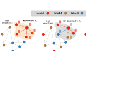
Figure 1: A toy example to show differences between conventional GNNs and our ES-GNN in aggregating node features. Conventional GNNs with local smoothness tend to produce non-discriminative representations on heterophilic graphs, while our ES-GNN is able to disentangle and exclude the task-harmful features from the final predictive target.

2 Preliminaries

Let $\mathcal{G}=(\mathcal{V},\mathcal{E})$ represents an undirected graph with adjacency matrix $\mathbf{A}\in\mathbb{R}^{|\mathcal{V}|\times|\mathcal{V}|}$, where $\mathcal{V}$ denotes the node set, $\mathcal{E}$ denotes the edge set, and $|\mathcal{V}|$ is the number of nodes. We define $(v_{i},v_{j})\in\mathcal{E}$, $v_{i},v_{j}\in\mathcal{V}$, $i\neq j$ if $v_{i}$ and $v_{j}$ are connected, and $\mathcal{N}_{i}=\{v_{j}|(v_{i},v_{j})\in\mathcal{E}\}$ as the neighborhood of node $v_{i}$. The nodes are associated with a feature matrix $\mathbf{X}\in\mathbb{R}^{|\mathcal{V}|\times f}$ where $f$ is the number of raw features, and we use $\mathbf{X}_{[i,:]}\in\mathbb{R}^{f}$ to denote the $i^{th}$ row of $\mathbf{X}$. We consider the standard node classification task on undirected graphs, where each node $v_{i}$ has a ground truth vector $\mathbf{y}_{i}\in\mathbb{R}^{C}$ in one-hot encoding where $\mathbf{y}_{i}(c_{i})=1$ and $c_{i}$ is the assigned label out of $C\leq|\mathcal{V}|$ classes. As our ES-GNN disentangles the original graph into the task-relevant and irrelevant subgraphs, we will denote their adjacency matrixes respectively as $\mathbf{A}_{\textit{R}}$ and $\mathbf{A}_{\textit{IR}}$ in this paper.

3 Background and Related Work

3.1 Homophily and Heterophily on Graphs

On graphs, homophily and heterophliy (or low homophily) typically refer to the similarity and dissimilarity between adjacent nodes, including but not limited to labels and features. In this work, we study node classification tasks, thereby focusing on homophily and heterophily in class labels. According to different homophily ratios, real-world networks in the literature, such as citation networks [26], social networks [27, 28], community networks [29, 30], webpage networks [27, 31], and co-occurrence networks [32] can be categorized into homophilic and heterophilc ones. Several metrics have been proposed to estimate the graph homophily level, e.g., edge homophily [10], as the most popular one, is defined as the percentage of edges linking nodes of the same label:

$$\mathcal{H}=\frac{|\{(v_{i},v_{j})|(v_{i},v_{j})\in\mathcal{E},\mathbf{y}_{i}=\mathbf{y}_{j}\}|}{|\mathcal{E}|}.$$ (1)

However, this metric may give inaccurate estimation in case of datasets with the class-imbalance problem [28]. To alleviate this, a new metric is proposed by [28]:

$$\centering\hat{\mathcal{H}}=\frac{1}{C-1}\sum^{C-1}_{k=0}\max(h_{k}-\frac{|\mathcal{C}_{k}|}{|\mathcal{V}|},0),\@add@centering$$ (2)

where $\mathcal{C}_{k}$ is the set of nodes from class $k\in\{0,1,...,C-1\}$, and $h_{k}$ is the class-wise homophily ratio computed as:

$$\centering h_{k}=\frac{\sum_{v_{i}\in\mathcal{C}_{k}}|\{v_{j}|\mathbf{y}_{i}=\mathbf{y}_{j},v_{j}\in\mathcal{N}_{i}\}|}{\sum_{v_{i}\in\mathcal{C}_{k}}|\mathcal{N}_{i}|}.\@add@centering$$ (3)

All these two indexes in Eq.(1) and Eq. (2) range from 0 to 1, of which the higher values suggest higher homophily (lower heterophily), and otherwise.

3.2 Graph Neural Networks

The central idea of most GNNs is to utilize nodes’ proximity information for building their representations for tasks, based on which great effort has been made in developing different variants [33, 24, 6, 34, 35, 36, 37, 38, 39, 40], and understanding the nature of GNNs [8, 9, 41, 42, 43, 44]. Several works have proved that GNNs essentially behave as a low pass filter that smooths information within node surrounding [6, 16, 45, 7]. In line with this view, [9] and [8] further show that a number of GNN models, such as GCN [33], SGC [6], GAT [24], and APPNP [46], can be seen as different optimization solvers to a graph signal denoising problem with a smoothness assumption upon connected nodes. All these results indicate that GNNs are mostly tailored for the strong homophily hypothesis on the observed graphs while largely overlooking the important setting of heterophily, where node features and labels vary unsmoothly on graphs. Recent studies [47, 20] also connect this to the over-smoothing problem [23].

To extend GNNs on heterophilic graphs, several works leverage the long-range information beyond nodes’ proximity. Geom-GCN [31] extends the standard message passing with geometric aggregation in latent space. H2GCN [10] directly models the higher order neighborhoods for capturing the homophily-dominant information. WRGAT [41] transforms the input graph into a multi-relational graph, for modeling structural information and enhancing the assortativity level. GEN [13] estimates a suitable graph for GNNs’ learning with multi-order neighborhood information and Bayesian inference as guide. Another line of work emphasizes the proper utilization of node neighbors. The most common works employ attention mechanism [24, 48], however, they are still imposing smoothness within nodes’ neighborhood albeit on the important members only [7, 9, 8]. Compared to that, FAGCN [18] adaptively models both similarities and dissimilarities between adjacent nodes. GPR-GNN [11] introduces a universal polynomial graph filter, by associating different hop neighbors with learnable weights in both positive and negative signs, so as to extract both low- and high-frequency information.

However, none of them analyzes the motivations why two nodes get connected, nor do they associate them with learning tasks, which is analyzed as one of the keys to generalize GNNs beyond homophily in this paper. In contrast, ES-GNN distinguishes graph edges as either relevant or irrelevant to the task. Such information acts as a guide to disentangle and exclude classification-harmful information from the final predictive target, and thus boosts GNNs’ performance under heterophily. Meanwhile, detailed analyses on the limited performance of the existing state-of-the-arts are provided in Section 6.3.

3.3 Disentangled Representation Learning

Disentangled representation learning is to learn decomposed vector representations which disentangle the explanatory latent variables underlying the observed data and encode them as separate dimensions [49, 50]. Existing efforts concerning that topic are mainly made on computer vision [51, 52, 53, 54], while a couple of works recently emerge to explore the potential of disentangled learning in graph-structured domains [55, 35, 56, 57]. For example, DisenGCN [55] employs a neighborhood routing mechanism to iteratively partition node neighborhood into multiple separated parts. FactorGCN [35] factorizes the original graph into multiple subgraphs by clipping edges so as to capture different graph aspects.

We notice that our work shares a similarity with FactorGCN [35]: to learn multiple subgraphs from the original network topology for disentangling features. Nevertheless, there are three main differences. First, FactorGCN could assign one edge to multiple groups, i.e., the factorized subgraphs may share overlapped edges, while our ES-GNN employs an edge splitting to partition the original network topology into two mutually exclusive ones satisfying $\mathbf{A}_{\textit{R}}+\mathbf{A}_{\textit{IR}}=\mathbf{A}$. Second, despite the disentangling property, FactorGCN merely interprets the inferred subgraphs as different graph aspects without providing any concrete meanings, and the predefined number of latent factors requires to be tuned differently across graphs. Differently, our model adaptively produces two interptable task-relevant and irrelevant topolgies for all kinds of input graphs. Last, FactorGCN models all disentangled parts towards final prediction, while we target at decoupling the task-relevant and task-irrelevant features whereby the classification-harmful information can be excluded from the final predictive target and disentangled in the task-irrelevant parts. Experimental results also validate that our proposed model substantially outperform FactorGCN on all the datasets used in the paper (see Section 6).

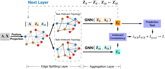
Figure 2: Illustration of our ES-GNN framework where $\mathbf{A}$ and $\mathbf{X}$ denote the adjacency matrix and feature matrix of nodes, respectively. First, $\mathbf{X}$ is projected onto different latent subspaces via different channels R and IR. An edge splitting is then performed to divide the original graph edges into two exclusive sets. After that, the node information can be aggregated individually and separately on different edge sets to produce disentangled representations, which are further utilized to make an more accurate edge splitting in the next layer. The task-relevant representation $\mathbf{Z}^{{}^{\prime}}_{\textit{R}}$ is reasonably granted for prediction. Meanwhile, an Irrelevant Consistency Regularization (ICR) is developed to further reduce the potential task-harmful information from the final predictive target.

4 Framework: ES-GNN

In this section, we propose an end-to-end graph learning framework, ES-GNN, generalizing Graph Neural Networks (GNNs) to arbitrary graph-structured data with either homophilic or heterophilic properties. An overview of ES-GNN is given in Fig. 2. The central idea is to integrate GNNs with an interpretable edge splitting (ES) layer that adaptively partitions the network topology as guide to disentangle the task-relevant and irrelevant node features.

4.1 Edge Splitting Layer

The goal of this layer is to infer the latent relations underlying adjacent nodes on the observed graph, and distinguish between graph edges which could be relevant or irrelevant to learning tasks. Given a simple graph with an adjacency matrix $\mathbf{A}$ and node feature matrix $\mathbf{X}$, an ES-layer splits the original graph edges into two exclusive sets, and thereby produces two partial network topologies with adjacency matrices $\mathbf{A}_{\text{{R}}},\mathbf{A}_{\text{{IR}}}\in\mathbb{R}^{|\mathcal{V}|\times|\mathcal{V}|}$ satisfying $\mathbf{A}_{\text{{R}}}+\mathbf{A}_{\text{{IR}}}=\mathbf{A}$. We would expect $\mathbf{A}_{\textit{R}}$ storing the most correlated graph edges to the classification task, of which the rest is excluded and disentangled in $\mathbf{A}_{\textit{IR}}$. Therefore, analyzing the correlation between node connections and learning tasks comes into the first step.

However, existing techniques [24, 25, 18] mainly parameterize graph edges with node similarity or dissimilarity, while failing to explicitly correlate them with the prediction target. Even worse, as the assortativiy of real-world networks is usually agnostic and node features are typically full of noises, the captured similarity/dissimilarity may not truly reflect the label-agreement/disagreement between nearby nodes. Consequently, the harmful-similarity between pairwise nodes from different classes could be mistakenly preserved for prediction. To this end, we present one plausible hypothesis below, whereby the explicit correlation between node connections and learning tasks is established automatically.

Hypothesis 1.

Two nodes get connected in a graph mainly due to their similarity in some features, which could be either relevant or irrelevant (even harmful) to the learning task.

This hypothesis is assumed without losing generality to both homophilic and heterophilic graphs. For a homophilic scenario, e.g., in citation networks, scientific papers tend to cite or be cited by others from the same area, and both of them usually possess the common keywords uniquely appearing in their topics. For a heterophilic scenario, students having different interests are likely be connected because of the same classes and/or dormitory they take and/or live in, but neither has direct relation to the clubs they have joined. This inspires us to classify graph edges by measuring the similarity between adjacent nodes in two different aspects, i.e., a graph edge is more relevant to classification task if the connected nodes are more similar in their task-relevant features, or otherwise. Our experimental analysis in Section 6.6 further provides evidences that even when our Hypothesis 1 may not hold, most adversarial edges (considered as the task-irrelevant ones) can still be recognized though neither types of node similarity exists.

It is worthy mentioning that our hypothesis is not in contradiction to the “opposites attract”, which could be intuitively explained by linking due to different but matching attributes. We believe the inherent cause to connection even in “opposites attract” may still be certain commonalities. For example, in heterosexual dating networks, people of the opposite sex are most likely connected because of their similar life values. Although these similarities may be inappropriate (or even harmful) in distinguishing genders, modeling and disentangling them from the final predictive target might be still of great importance.

An ES-layer consists of two channels to respectively extract the task-relevant and irrelevant information from nodes. As only the raw feature matrix $\mathbf{X}$ is provided in the beginning, we will project them into two different subspaces before the first ES-layer:

$$\mathbf{Z}_{s}^{(0)}=\sigma(\mathbf{W}_{s}^{T}\mathbf{X}+\mathbf{b}_{s}),$$ (4)

where $\mathbf{W}_{s}\in\mathbb{R}^{f\times\frac{d}{2}}$ and $\mathbf{b}_{s}\in\mathbb{R}^{\frac{d}{2}}$ are the learnable parameters in channel $s\in\{\textit{R},\textit{IR}\}$, $d$ is the number of node hidden states, and $\sigma$ is a nonlinear activation function.

Given Hypothesis 1, a graph edge should be classified into the task-relevant set if the connected nodes display a higher similarity in the corresponding channel, and otherwise. However, introducing metrics between nearby nodes to learn $\mathbf{A}_{\textit{R}}$ and $\mathbf{A}_{\textit{IR}}$ independently may fail to model the complex interaction between different channels, and also lose emphasis on topology difference. Therefore, in case of $\mathbf{A}_{(i,j)}=1$, we parameterize the residual between $\mathbf{A}_{\textit{R}(i,j)}$ and $\mathbf{A}_{\textit{IR}(i,j)}$, and solving the linear equation:

$$\begin{cases}\mathbf{A}_{\textit{R}(i,j)}-\mathbf{A}_{\textit{IR}(i,j)}=\alpha_{i,j}\\ \mathbf{A}_{\textit{R}(i,j)}+\mathbf{A}_{\textit{IR}(i,j)}=1\end{cases}.$$ (5)

This gives us $\mathbf{A}_{\textit{R}(i,j)}=\frac{1+\alpha_{i,j}}{2}$ and $\mathbf{A}_{\textit{IR}(i,j)}=\frac{1-\alpha_{i,j}}{2}$ with $\alpha_{i,j}\in\left(-1,1\right)$. To effectively incorporate all the channel information into the coefficient $\alpha_{i,j}$, we propose a residual scoring mechanism:

$$\alpha_{i,j}=\tanh(\mathbf{g}\left[\mathbf{Z}_{\textit{R}[i,:]}\oplus\mathbf{Z}_{\textit{IR}[i,:]}\oplus\mathbf{Z}_{\textit{R}[j,:]}\oplus\mathbf{Z}_{\textit{IR}[j,:]}\right]^{T}).$$ (6)

Here, both of the task-relevant and irrelevant node features are first concatenated and convoluted by learnable $\mathbf{g}\in\mathbb{R}^{1\times 2d}$, and then passed to the tangent activation function to produce a scalar value within $\left(-1,1\right)$. To further strengthen the discreteness property of (or exclusiveness between) $\mathbf{A}_{\textit{R}}$ and $\mathbf{A}_{\textit{IR}}$, one can apply techniques, such as softmax with temperature in Eq. (7), Gumbel-Softmax [58, 59] in Eq. (8), or threholding in Eq. (9).

$$\mathbf{A}_{\textit{s}(i,j)}^{{}^{\prime}} =\frac{\exp(\mathbf{A}_{\textit{s}(i,j)}/\tau)}{\sum_{\kappa\in\{\textit{R},\textit{IR}\}}\exp(\mathbf{A}_{\kappa(i,j)}/\tau)}$$ (7)

$$\mathbf{A}_{\textit{s}(i,j)}^{{}^{\prime}} =\frac{\exp((\log(\mathbf{A}_{\textit{s}(i,j)})+\gamma)/\tau)}{\sum_{\kappa\in\{\textit{R},\textit{IR}\}}\exp((\log(\mathbf{A}_{\kappa(i,j)})+\gamma)/\tau)}$$ (8)

$$\mathbf{A}_{\textit{s}(i,j)}^{{}^{\prime}} =\begin{cases}1&\mathbf{A}_{\textit{s}(i,j)}>0.5\\ 0&\text{otherwise}\end{cases}$$ (9)

where $s\in\{\textit{R},\textit{IR}\}$, $\tau$ is a hyper-parameter mediating discreteness degree, and $\gamma\sim\textit{Gumbel}(0,1)$ is a Gumbel random variable. However, in this work, we find good results without adding any additional discretization techniques, and will leave this investigation to the future work.

4.2 Aggregation Layer

As the split network topologies disclose the partial relations among nodes in different latent spaces, they can be utilized to aggregate information for learning different node aspects. Specifically, we leverage a simple low-pass filter with scaling parameters $\{\epsilon_{\textit{R}},\epsilon_{\textit{IR}}\}$ for both task-relevant and irrelevant channels, from the $k^{th}$ to $k+1^{th}$ layer:

$$\mathbf{Z}_{s}^{(k+1)}=\epsilon_{s}\mathbf{Z}_{s}^{(0)}+(1-\epsilon_{s})\mathbf{D}^{-\frac{1}{2}}_{s}\mathbf{A}_{s}\mathbf{D}^{-\frac{1}{2}}_{s}\mathbf{Z}_{s}^{(k)}.$$ (10)

$s\in\{\textit{R},\textit{IR}\}$ denotes the task-relevant or irrelevant channel, and $\mathbf{D}_{s}$ is the degree matrix associated with the adjacency matrix $\mathbf{A}_{s}$. Derivation of Eq. (10) is detailed in our theoretical analysis. Importantly, by incorporating proximity information in different structural spaces, the task-relevant and irrelevant information can be better disentangled in $\mathbf{Z}_{\text{{R}}}^{(k+1)}$ and $\mathbf{Z}_{\textit{IR}}^{(k+1)}$, based on which the next ES-layer can make a more precise partition on the raw topology.

Algorithm 1 Framework of ES-GNN

0:  nodes set: $\mathcal{V}$, edge set: $\mathcal{E}$, adjacency matrix: $\mathbf{A}\in\mathbb{R}^{|\mathcal{V}|\times|\mathcal{V}|}$, node feature matrix: $\mathbf{X}\in\mathbb{R}^{|V|\times f}$, the number of layers: $K$, scaling parameters: $\{\epsilon_{\textit{R}},\epsilon_{\textit{IR}}\}$, irrelevant consistency coefficient: $\lambda_{\text{ICR}}$, and ground truth labels on the training set: $\{\mathbf{y}_{i}\in\mathbb{R}^{C}|\forall v_{i}\in\mathcal{V}_{\text{trn}}\}$.

0:  $\mathbf{W}_{\textit{R}},\mathbf{W}_{\textit{IR}}\in\mathbb{R}^{f\times d}$, $\mathbf{W}_{F}\in\mathbb{R}^{d\times C},\mathbf{b}_{F}\in\mathbb{R}^{C}$, $\{\mathbf{g}^{(k)}\in\mathbb{R}^{1\times 2d}|k=0,1,...,K-1\}$

1:  // Project node features into two subspaces.

2:  for $s\in\{\text{{R}},\text{{IR}}\}$ do

3:     $\mathbf{Z}_{s}^{(0)}\leftarrow\sigma(\mathbf{W}_{s}^{T}\>\mathbf{X}+\mathbf{b}_{s})$.

4:     $\mathbf{Z}_{s}^{(0)}\leftarrow\text{Dropout}(\mathbf{Z}_{s}^{(0)})$ // Enabled only for training.

5:  end for

6:  // Stack Edge Splitting and Aggregation Layers.

7:  for layer number $k=0,1,...,K-1$ do

8:     // Edge Splitting Layer.

9:     Initialize $\mathbf{A}_{\textit{R}},\mathbf{A}_{\textit{IR}}\in\mathbb{R}^{|\mathcal{V}|\times|\mathcal{V}|}$ with zeros.

10:     for $\left(v_{i},v_{j}\right)\in\mathcal{E}$ do

11:        $\alpha_{i,j}\leftarrow\tanh({\mathbf{g}^{(k)}}\left[\mathbf{Z}_{{\text{{R}}}[i,:]}^{(k)}\oplus\mathbf{Z}_{{\text{{IR}}}[i,:]}^{(k)}\oplus\mathbf{Z}_{{\text{{R}}}[j,:]}^{(k)}\oplus\mathbf{Z}_{\textit{IR},[j,:]}^{(k)}\right]^{T})$.

12:        $\alpha_{i,j}\leftarrow\text{Dropout}(\alpha_{i,j})$ // Enabled only for training.

13:        $\mathbf{A}_{\textit{R}(i,j)}\leftarrow\frac{1+\alpha_{i,j}}{2}$, $\mathbf{A}_{\textit{IR}(i,j)}\leftarrow\frac{1-\alpha_{i,j}}{2}$.

14:     end for

15:     // Aggregation Layer.

16:     for $s\in\{{\text{{R}}},\text{{IR}}\}$ do

17:        $\mathbf{Z}_{s}^{(k+1)}\leftarrow\epsilon_{s}\mathbf{Z}_{s}^{(0)}+(1-\epsilon_{s})\mathbf{D}^{-\frac{1}{2}}_{s}\mathbf{A}_{s}\mathbf{D}^{-\frac{1}{2}}_{s}\mathbf{Z}_{s}^{(k)}$.

18:     end for

19:  end for

20:  // Prediction.

21:  $\hat{\mathbf{y}}_{i}=\text{softmax}(\mathbf{W}_{F}^{T}\mathbf{Z}_{{\text{{R}}}[i,:]}^{(K)}+\mathbf{b}_{F}),\forall v_{i}\in\mathcal{V}$.

22:  // Optimization with Irrelevant Consistency Regularization.

23:  $\mathcal{L}_{\text{ICR}}=\sum_{(v_{i},v_{j})\in\mathcal{E}}(1-\delta(\hat{\mathbf{y}}_{i},\hat{\mathbf{y}}_{j}))\|\mathbf{Z}_{\text{{IR}}[i,:]}-\mathbf{Z}_{\text{{IR}}[j,:]}\|_{2}^{2}$.

24:  $\mathcal{L}_{\text{pred}}=-\frac{1}{|\mathcal{V}_{\text{trn}}|}\sum_{i\in\mathcal{V}_{\text{trn}}}\mathbf{y}_{i}^{T}\log(\hat{\mathbf{y}}_{i})$.

25:  Minimize $\mathcal{L}_{\text{pred}}+\lambda_{\text{ICR}}\mathcal{L}_{\text{ICR}}$.

4.3 Irrelevant Consistency Regularization

Stacking ES-layer and aggregation layer iteratively lends itself to disentangling different features of nodes into the task-relevant and irrelevant representations, denoted by $\mathbf{Z}_{\text{{R}}}$ and $\mathbf{Z}_{\text{{R}}}$ respectively. First, $\mathbf{Z}_{\text{{R}}}$ is granted for prediction and gradually trained by the supervision signals from the classification loss. However, only supervising one channel (R) may not also guarantee the meaningfulness of the other (IR), which possibly results in inaccurate disentanglement. The confounding and erroneous information could then be mistakenly preserved for prediction. To this end, we propose to regulate $\mathbf{Z}_{\text{{IR}}}$ for modeling the opposite of $\mathbf{Z}_{\text{{R}}}$, i.e., the classification-harmful information hidden in the observed graph.

To attain this, we develop Irrelevant Consistency Regularization (ICR) that imposes a concrete meaning on $\mathbf{Z}_{\text{{IR}}}$. The rationale is to incorporate the potential label-disagreement between adjacent nodes into $\mathbf{Z}_{\text{{IR}}}$. Given any two connected nodes $v_{i}$ and $v_{j}$, we would expect $\mathbf{Z}_{{\text{{IR}}}[i,:]}$ and $\mathbf{Z}_{{\text{{IR}}}[j,:]}$ to be similar if they share a distinct label. Specifically, our ICR can be formulated as:

$$\mathcal{L}_{\text{ICR}}=\sum_{(v_{i},v_{j})\in\mathcal{E}}(1-\delta(\mathbf{y}_{i},\mathbf{y}_{j}))\|\mathbf{Z}_{\text{{IR}}[i,:]}-\mathbf{Z}_{\text{{IR}}[j,:]}\|_{2}^{2},$$ (11)

where $\delta$ is a Kronecker function returning 1 if $\mathbf{y}_{i}=\mathbf{y}_{j}$ and 0 otherwise, and $\|\cdot\|_{2}$ denotes $l_{2}$ norm. By doing so, $\mathbf{Z}_{{\text{{IR}}}}$ is constrained with a local consistency between adjacent nodes from different classes. As a benefit, the classification-harmful similarity between nodes can be further excluded from $\mathbf{Z}_{\text{{R}}}$, and disentangled in $\mathbf{Z}_{\text{{IR}}}$.

Several powerful techniques [60, 25] have been developed to measure the label-agreement between pairwise nodes. In this work, however, we find that using directly the joint probability from model prediction works well, which also offers advantages in low computational complexity as no additional trainable parameters are required.

4.4 Overall Algorithm

The overall pipeline of ES-GNN is detailed in Algorithm 1. Specifically, we adopt ReLU activation function in Eq. (4) to first map node features into two different channels, and then pass them with the adjacency matrix to an ES-layer for splitting the raw network topology into two exclusive parts. After that, these two partial network topologies are utilized to aggregate information in different structural spaces. Alternatively stacking ES-layer and aggregation layer not only enables more accurate disentanglement but also explores the graph information beyond local neighborhood. Finally, a fully connected layer is appended to project the learned representations into class space $\mathbb{R}^{C}$. We integrate $\mathcal{L}_{\text{ICR}}$ into the optimization process with a irrelevant consistency coefficient $\lambda_{\text{ICR}}$ to have final objective function below, where $\mathcal{L}_{\text{pred}}=-\frac{1}{|\mathcal{V}_{\text{trn}}|}\sum_{v_{i}\in\mathcal{V}_{\text{trn}}}\mathbf{y}_{i}^{T}\log(\hat{\mathbf{y}}_{i})$.

$$\mathcal{L}=\mathcal{L}_{\text{pred}}+\lambda_{\text{ICR}}\mathcal{L}_{\text{ICR}}.$$ (12)

Finally, we also report in Table I the complexity of the proposed ES-GNN method in comparison with the state-of-the-arts which will be evaluated in the experimental section. Clearly, our model displays the same complexity to FAGCN [18] while being slightly overhead compared to GPR-GNN [11]. Here, we omit the related works, GEN [13] and WRGAT [14], as their complexity is obviously higher than others by involving reconstructing the whole graph.

TABLE I: Time complexity of the comparison models with one hidden layer as an example. $N_{e}$ denotes the number of graph aspects assumed in FactorGCN [35], $D_{\text{max}}$ represents the maximum node degree, and $|\mathcal{E}_{2}|$ is the total number of neighbors in the second hop of nodes. Other symbols are earlier defined in the texts.

Models	Complexity
GCN [33]	$\mathcal{O}((f+C)|\mathcal{E}|d)$
GAT [24]	$\mathcal{O}(((2+f)|\mathcal{V}|+(4+C)|\mathcal{E}|)d)$
FactorGCN [35]	$\mathcal{O}(N_{e}|\mathcal{V}|+(|\mathcal{V}|f+(3+C)|\mathcal{E}|)d)$
H2GCN [10]	$\mathcal{O}(fd+|\mathcal{E}|D_{\text{max}}+(|\mathcal{E}|+|\mathcal{E}_{2}|)d)$
FAGCN [18]	$\mathcal{O}(((1+C+f)|\mathcal{V}|+|\mathcal{E}|)d)$
GPR-GNN [11]	$\mathcal{O}((f|\mathcal{V}|+|\mathcal{E}|C)d)$
ES-GNN (Ours)	$\mathcal{O}(((1+C+f)|\mathcal{V}|+|\mathcal{E}|)d)$

5 Theoretical Analysis

In this section, we investigate two important problems: (1) what limits the generalization power of the conventional GNNs on graphs beyond homophily, and (2) how the proposed ES-GNN breaks this limit and performs well on different types of networks. We will answer these questions by first analyzing the typical GNNs as graph signal denoising from a more generalized viewpoint, and then impose our Hypothesis 1 to derive ES-GNN.

5.1 Limited Generalization of Conventional GNNs

Recent studies [9, 8] have proved that most GNNs can be regarded as solving a graph signal denoising problem:

$$\mathop{\arg\min}_{\mathbf{Z}}\ \ \|\mathbf{Z}-\mathbf{X}\|^{2}_{2}+\xi\cdot tr(\mathbf{Z}^{T}\mathbf{L}\mathbf{Z}),$$ (13)

where $\mathbf{X}\in\mathbb{R}^{|\mathcal{V}|\times f}$ is the input signal, $\mathbf{L}=\mathbf{D}-\mathbf{A}\in\mathbb{R}^{|\mathcal{V}|\times|\mathcal{V}|}$ is the graph laplacian matrix, and $\xi$ is a constant coefficient. The first term guides $\mathbf{Z}$ to be close to $\mathbf{X}$, while the second term $tr(\mathbf{Z}^{T}\mathbf{L}\mathbf{Z})$ is the laplacian regularization, which enforces smoothness between connected nodes. One fundamental assumption made here is that similar nodes should have a higher tendency to connect each other, and we refer it as standard smoothness assumption on graphs. However, real-world networks typically exhibit diverse linking patterns of both assortativity and disassortativity. Constraining smoothness on each node pair is prone to mistakenly preserve both of the task-relevant and irrelevant (or even harmful) information for prediction. Given that, we divide the original graph into two subgraphs with the same nodes sets but exclusive edge sets, and reformulate Eq. (13) as:

$$\centering\begin{split}\mathop{\arg\min}_{\mathbf{Z}}\ \ \|\mathbf{Z}-\mathbf{X}\|^{2}_{2}+\xi\cdot tr(\mathbf{Z}^{T}\mathbf{L}_{\text{{R}}}\mathbf{Z})+\xi\cdot tr(\mathbf{Z}^{T}\mathbf{L}_{\text{{IR}}}\mathbf{Z}).\end{split}\@add@centering$$ (14)

Here, $\mathbf{L}_{\text{{R}}}=\mathbf{D}_{\text{{R}}}-\mathbf{A}_{\text{{R}}}$, and $\mathbf{L}_{\text{{IR}}}=\mathbf{D}_{\text{{IR}}}-\mathbf{A}_{\text{{IR}}}$, where the task-relevant and irrelevant node relations are separately captured in $\mathbf{A}_{\text{{R}}}$ and $\mathbf{A}_{\text{{IR}}}$. Clearly, emphasizing the commonality between adjacent nodes in $\mathbf{A}_{\text{{R}}}$ is beneficial for keeping task-correlated information only. However, smoothing node pairs in $\mathbf{A}_{\text{{IR}}}$ simultaneously may preserve classification-harmful similarity between nodes, thus limiting the prediction performance of GNNs.

5.2 Disentangled Smoothness Assumption in ES-GNN

Our Hypothesis 1 suggests that the original graph topology can be partitioned into two exclusive ones, wherein connected nodes displays high similarity with either task-relevant or irrelevant features only. We further interpret this result as disentangled smoothness assumption, based on which the conventional graph signal denoising problem in Eq. (13) can be generalized as:

$$\mathop{\arg\min}_{\mathbf{Z}_{\textit{R}},\mathbf{Z}_{\textit{IR}}} \|\mathbf{Z}_{\textit{R}}-\mathbf{X}_{\textit{IR}}\|^{2}_{2}+\|\mathbf{Z}_{\text{{IR}}}-\mathbf{X}_{\text{{IR}}}\|^{2}_{2}$$ (15)

$$+\xi\cdot tr(\mathbf{Z}^{T}_{\textit{R}}\mathbf{L}_{\textit{R}}\mathbf{Z}_{\textit{R}})+\xi\cdot tr(\mathbf{Z}^{T}_{\textit{IR}}\mathbf{L}_{\textit{IR}}\mathbf{Z}_{\textit{IR}})$$

where $$\mathbf{L}_{\textit{R}}=\mathbf{D}_{\textit{R}}-\mathbf{A}_{\textit{R}},\mathbf{L}_{\textit{IR}}=\mathbf{D}_{\textit{IR}}-\mathbf{A}_{\textit{IR}}$$

s.t. $$\mathbf{A}_{\textit{R}}+\mathbf{A}_{\textit{IR}}=\mathbf{A}$$

$$\mathbf{A}_{\textit{R}(i,j)},\mathbf{A}_{\textit{IR}(i,j)}\in[0,1].$$

Here, $\mathbf{A}_{\textit{R}(i,j)}$ and $\mathbf{A}_{\textit{IR}(i,j)}$ measure the degree to which the node connection $(v_{i},v_{j})$ are relevant and irrelevant to the learning task, respectively. We further name this optimization as disentangled graph denoising problem, and finally derive the following theorem:

Theorem 1.

The proposed ES-GNN is equivalent to the solution of the disentangled graph denoising problem in Eq. (15).

Proof.

Let $\mathbf{X}_{\text{{R}}}\in\mathbb{R}^{\frac{d}{2}}$ and $\mathbf{X}_{\text{{IR}}}\in\mathbb{R}^{\frac{d}{2}}$ be the results of mapping $\mathbf{X}$ into different channels in Eq. (4), i.e., $\mathbf{X}_{\text{{R}}}=\mathbf{Z}_{\text{{R}}}^{(0)}$ and $\mathbf{X}_{\text{{IR}}}=\mathbf{Z}_{\text{{IR}}}^{(0)}$. Hypothesis 1 motivates us to define $\mathbf{A}_{\textit{R}(i,j)}$ and $\mathbf{A}_{\textit{IR}(i,j)}$ as node similarity in two aspects. Combining above constraints, we have a linear system in case of $\mathbf{A}_{(i,j)}=1$:

$$\begin{cases}\mathbf{A}_{\textit{R}(i,j)}+\mathbf{A}_{\textit{IR}(i,j)}=1\\ \mathbf{A}_{\textit{R}(i,j)}-\mathbf{A}_{\textit{IR}(i,j)}=\phi_{\text{res}}(\mathbf{Z}_{\textit{R}[i,:]},\mathbf{Z}_{\textit{IR}[i,:]},\mathbf{Z}_{\textit{R}[j,:]},\mathbf{Z}_{\textit{IR}[j,:]})\end{cases},$$ (16)

where $\phi_{\text{res}}(\cdot)$ outputs the residual between $\mathbf{A}_{\textit{R}(i,j)}$ and $\mathbf{A}_{\textit{IR}(i,j)}$ considering both task-relevant and irrelevant node information, and can be formulated with our residual scoring mechanism in Eq. (6). Solving above equations, we can express both $\mathbf{A}_{\textit{R}}$ and $\mathbf{A}_{\textit{IR}}$ in terms of $\mathbf{Z}_{\textit{R}}$ and $\mathbf{Z}_{\textit{IR}}$, i.e.,

$$\mathbf{A}_{\textit{R}(i,j)} =\frac{1+\phi_{\text{res}}(\mathbf{Z}_{\textit{R}[i,:]},\mathbf{Z}_{\textit{IR}[i,:]},\mathbf{Z}_{\textit{R}[j,:]},\mathbf{Z}_{\textit{IR}[j,:]})}{2}$$ (17)

$$\mathbf{A}_{\textit{IR}(i,j)} =\frac{1-\phi_{\text{res}}(\mathbf{Z}_{\textit{R}[i,:]},\mathbf{Z}_{\textit{IR}[i,:]},\mathbf{Z}_{\textit{R}[j,:]},\mathbf{Z}_{\textit{IR}[j,:]})}{2}.$$ (18)

So far, the optimization problem in Eq. (15) is only made up of variables $\mathbf{X}_{\textit{R}}$, $\mathbf{X}_{\textit{IR}}$, $\mathbf{Z}_{\textit{R}}$, and $\mathbf{Z}_{\textit{IR}}$. Directly solving it is still however not easy, as the mixing variables of $\mathbf{Z}_{\textit{R}}$ and $\mathbf{Z}_{\textit{IR}}$, and the introduced non-linear operator in $\phi_{\text{res}(\cdot)}$ result in a complicated differentiation process.

Instead, we can approach this problem by decoupling the learning of $\mathbf{A}_{\textit{R}},\mathbf{A}_{\textit{IR}}$ from the optimization target, and employ an alternative learning between stages. Suppose we have attained the task-relevant and irrelevant node features in the $k^{th}$ round, i.e., $\mathbf{Z}_{\textit{R}}^{(k)}$ and $\mathbf{Z}_{\textit{IR}}^{(k)}$. In the first stage, we can compute $\mathbf{A}_{\textit{R}(i,j)}^{(k+1)}$ and $\mathbf{A}_{\textit{IR}(i,j)}^{(k+1)}$ using $\{\mathbf{Z}_{\text{{R}}[i,:]}^{(k)},\mathbf{Z}_{\text{{IR}}[i,:]}^{(k)},\mathbf{Z}_{\text{{R}},[j,:]}^{(k)},\mathbf{Z}_{\text{{IR}}[j,:]}^{(k)}\}$ with Eq. (17) and Eq. (18), which in fact turns out to be our ES-layer in Section 4.1.

In the second stage, injecting the computed values of $\mathbf{A}_{\textit{R}(i,j)}^{(k+1)}$ and $\mathbf{A}_{\textit{IR}(i,j)}^{(k+1)}$ relaxes the mixture of variables $\mathbf{Z}_{\textit{R}}$ and $\mathbf{Z}_{\textit{IR}}$, and the original optimization problem can then be disentangled into two independent targets (as all four penalized terms are positive):

$$\mathop{\arg\min}_{\mathbf{Z}_{\text{{R}}}^{*}}\|\mathbf{Z}_{\text{{R}}}^{*}-\mathbf{Z}_{\text{{R}}}^{(0)}\|^{2}_{2}+\xi\cdot tr({\mathbf{Z}_{\text{{R}}}^{*}}^{T}\mathbf{L}_{\text{{R}}}^{(k)}\mathbf{Z}_{\text{{R}}}^{*})$$ (19)

$$\mathop{\arg\min}_{\mathbf{Z}_{\text{{IR}}}^{*}}\|\mathbf{Z}_{\text{{IR}}}^{*}-\mathbf{Z}_{\text{{IR}}}^{(0)}\|^{2}_{2}+\xi\cdot tr({\mathbf{Z}_{\text{{IR}}}^{*}}^{T}\mathbf{L}_{\text{\text{{IR}}}}^{(k)}\mathbf{Z}_{\text{{IR}}}^{*})$$ (20)

where $\mathbf{L}_{\textit{R}}^{(k)}=\mathbf{D}_{\textit{R}}^{(k)}-\mathbf{A}_{\textit{R}}^{(k)}$ and $\mathbf{L}_{\textit{IR}}^{(k)}=\mathbf{D}_{\textit{IR}}^{(k)}-\mathbf{A}_{\textit{IR}}^{(k)}$ are fixed values. Lemma 1, on the R channel as an example, further shows that our aggregation layer, on the task-relevant and irrelevant topologies, in Section 4.2 is approximately solving these two optimization problems in Eq. (19) and Eq. (20).

Therefore, stacking ES- and aggregation layers iteratively is equivalent to the above alternative learning for solving the disentangled graph denoising problem in Eq. (15) with $\mathbf{X}_{\textit{R}}=\mathbf{Z}_{\textit{R}}^{(0)}$ and $\mathbf{X}_{\textit{IR}}=\mathbf{Z}_{\textit{IR}}^{(0)}$. Finally, given $\mathbf{Z}_{\text{{R}}}^{(K)}$ and $\mathbf{Z}_{\text{{IR}}}^{(K)}$, we minimize the prediction loss $\mathcal{L}_{\text{pred}}$ and the Irrelevant Consistency Regularization $\mathcal{L}_{\text{ICR}}$ in Eq. (12) with Adam [61] algorithm, which imposes concrete meanings on different channels, and simultaneously ensures the convergence of our described alternative learning. ∎

Lemma 1.

When adopting the normalized laplacian matrix $\mathbf{L}_{\text{{R}}}=\mathbf{I}-\mathbf{D}_{\text{{R}}}^{-\frac{1}{2}}\mathbf{A}_{\text{{R}}}\mathbf{D}_{\text{{R}}}^{-\frac{1}{2}}$, the feature aggregation operator in Eq. (10) with channel $s=\text{{R}}$ can be regarded as solving Eq. (19) using iterative gradient descent with stepsize $\beta=\frac{1}{2+2\xi}$ and $\xi=\frac{1}{\epsilon_{\text{{R}}}}-1$.

Proof.

We take iterative gradient descent with the stepsize $\beta$ to solve the denoising problem in Eq. (19) (referred as $\mathcal{L}_{\textit{R}}$) as follows:

$$\mathbf{Z}_{\textit{R}}^{(k+1)} =\mathbf{Z}_{\textit{R}}^{(k)}-\beta\cdot\dfrac{\partial\mathcal{L}_{\textit{R}}}{\partial\mathbf{Z}_{\textit{R}}^{*}}|_{\mathbf{Z}_{\textit{R}}^{*}=\mathbf{Z}_{\textit{R}}^{(k)}}$$ (21)

$$=2\beta\mathbf{Z}_{\textit{R}}^{(0)}+2\beta\xi(\mathbf{D}_{\textit{R}}^{-\frac{1}{2}}\mathbf{A}_{\textit{R}}\mathbf{D}_{\textit{R}}^{-\frac{1}{2}})\mathbf{Z}_{\textit{R}}^{(k)}+(1-2\beta-2\beta\xi)\mathbf{Z}_{\textit{R}}^{(k)}.$$ (22)

Setting $\beta$ as $\frac{1}{2+2\xi}$ gives us:

$$\mathbf{Z}_{\textit{R}}^{(k+1)}=\frac{1}{1+\xi}\mathbf{Z}_{\textit{R}}^{(0)}+\frac{\xi}{1+\xi}(\mathbf{D}_{\textit{R}}^{-\frac{1}{2}}\mathbf{A}_{\textit{R}}\mathbf{D}_{\textit{R}}^{-\frac{1}{2}})\mathbf{Z}_{\textit{R}}^{(k)},$$ (23)

which is equivalent to Eq. (10) while choosing $\xi=\frac{1}{\epsilon_{\textit{R}}}-1$, i.e.,

$$\mathbf{Z}_{\textit{R}}^{(k+1)}=\epsilon_{\textit{R}}\mathbf{Z}_{\textit{R}}^{(0)}+(1-\epsilon_{\textit{R}})(\mathbf{D}_{\textit{R}}^{-\frac{1}{2}}\mathbf{A}_{\textit{R}}\mathbf{D}_{\textit{R}}^{-\frac{1}{2}})\mathbf{Z}_{\textit{R}}^{(k)}.$$ (24)

∎

As the possible classification-harmful similarity between nodes (hidden in $\mathbf{A}_{\textit{IR}}$) can be excluded from $\mathbf{Z}_{\textit{R}}$ and disentangled in $\mathbf{Z}_{\textit{IR}}$ while optimizing Eq. (15), our ES-GNN presents a universal approach that theoretically guarantees good performance on different types of networks.

TABLE II: Statistics of real-world datasets, where $\mathcal{H}$ and $\hat{\mathcal{H}}$ (considering class-imbalance problem) provide indexes of graph homophily ratio as respectively defined in Eq. (1) and Eq. (2). It can be observed that, despite the relative high homophily level measured by $\mathcal{H}=0.632$, the Twitch-DE dataset with class-imbalance problem is essentially a heterophilic graph [28] as suggested by $\hat{\mathcal{H}}=0.139$. For Polblogs dataset, since node features are not provided, we directly use the rows of the adjacency matrix.

Datasets	Heterophilic Graphs							Homophilic Graphs
	Squirrel	Chameleon	Wisconsin	Cornell	Texas	Twitch-DE	Actor	Cora	Citeseer	Pubmed	Polblogs
$\mathcal{H}$	0.222	0.230	0.178	0.296	0.061	0.632	0.217	0.810	0.735	0.802	0.906
$\hat{\mathcal{H}}$	0.025	0.062	0.094	0.047	0.001	0.139	0.011	0.766	0.627	0.664	0.811
# Nodes	5,201	2,277	251	183	183	9,498	7,600	2,708	3,327	19,717	1,222
# Edges	217,073	36,101	499	295	309	153,138	33,544	5,429	4,732	44,338	16,714
# Features	2,089	2,325	1,703	1,703	1,703	2,514	931	1,433	3,703	500	/
# Classes	5	5	5	5	5	2	5	7	6	3	2

6 Experiments

We empirically evaluate our ES-GNN for node classification using both synthetic and real-world datasets in this section.

6.1 Datasets & Experimental Setup

6.1.1 Real-World Datasets

We consider 11 widely used benchmark datasets including both seven heterophilc graphs, i.e., Chameleon, Squirrel [27], Wisconsin, Cornell, Texas [31] (webpage networks), Actor [32] (co-occurrence network), and Twitch-DE [27, 28] (social network), as well as four homophilic graphs including Cora, Citeseer, Pubmed [26] (citation networks), and Polblogs [29, 30] (community network) with statistics shown in Table II.

6.1.2 Synthetic Data

To investigate the behavior of GNNs on graphs with arbitrary levels of homophily and heterophily, we construct synthetic graphs with our Hypothesis 1. The central idea is to define links among nodes under two conditions independently, of which only one is correlated with the classification task. We consider 1,200 nodes, 3 equal-size classes, and 500 node features made up of both explicit and implicit attributes. The explicit attributes depend on the label assignment, while the implicit ones model dependency across different classes. Fig. 3 further illustrates their allocation to nodes in the step-2 with shape and color as an example. Notably, all these attributes in six types (three explicit and three implicit ones) are randomly sampled from different Gaussian distributions, each pair of them are combined via element-wise addition to attain the final node features. For instance, the features of a node (from class-$i$) with explicit attribute-$i$ and implicit attribute-$j$ are defined as the addition of two random vectors respectively sampled from $\mathcal{N}(\boldsymbol{\mu}_{\text{E},i},\boldsymbol{\sigma}_{\text{E},i})$ and $\mathcal{N}(\boldsymbol{\mu}_{\text{I},j},\boldsymbol{\sigma}_{\text{I},j})$, where $\boldsymbol{\mu}_{\text{E},i},\boldsymbol{\mu}_{\text{I},j}\in\mathbb{R}^{f_{\text{syn}}}$ are means, $\boldsymbol{\sigma}_{\text{E},i},\boldsymbol{\sigma}_{\text{I},j}\in\mathbb{R}^{f_{\text{syn}}\times f_{\text{syn}}}$ are the associated covariance matrixes, and $f_{\text{syn}}=500$ is the feature dimensions.

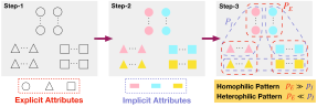
Figure 3: Constructing synthetic graphs with arbitrary levels of homophily and heterophily. Shape and color of nodes respectively illustrate the explicit and implicit node attributes. Nodes with the same shape or color are connected with a probability of $P_{\text{E}}$ or $P_{\text{I}}$, independently, while they are only classified by their shapes (the explicit attributes) into three categories. Obviously, we can observe heterophilic graph pattern given $P_{\text{E}}\ll P_{\text{I}}$, and strong homophily otherwise.

After that, inspired by the Erdős-Rényi random graphs, we connect nodes with probability $P_{\text{E}}$ if they are from the same class (the task-relevant condition), with probability $P_{\text{I}}$ if they share different labels but posses implicit attributes from the same distribution (the task-irrelevant condition), as shown in Fig. 3 (see step-3). For all other cases, we connect nodes with probability $q$ in a small value, $1\mathrm{e}{-5}$ in this work for ensuring a connected graph. Since no class-imbalance problem exists here, the homophily ratios of our generated graphs are measured with Eq. (1). Intuitively, we could anticipate heterophilic connecting pattern when setting $P_{\text{E}}\ll P_{\text{I}}$, and strong homophily otherwise. Quantitatively, the relationship between the homophily ratio $\mathcal{H}_{\text{syn}}$ and parameters $P_{\text{E}}$, $P_{\text{I}}$ can be derived with the simple knowledge on combinatorics and statistics while omitting the small value of $q$:

$$\mathcal{H}_{\text{syn}}(P_{\text{E}},P_{\text{I}})=\frac{3(n-3)}{3(n-3)+2n\frac{P_{\text{I}}}{P_{\text{E}}}},$$ (25)

with $n$ being the total number of nodes. Clearly, we have $\mathcal{H}_{\text{syn}}\to 0$ while $P_{\text{I}}\gg P_{\text{E}}$, and $\mathcal{H}_{\text{syn}}\to 1$ while $P_{\text{I}}\ll P_{\text{E}}$. To avoid possible computational overhead, we also need to control the average node degree of our synthetic graphs. Similarly, we can approximately derive it as the function of $P_{\text{I}}$ and $P_{\text{E}}$:

$$\mathcal{T}(P_{\text{E}},P_{\text{I}})=\frac{n-3}{3}P_{\text{E}}+\frac{4n}{9}P_{\text{I}}.$$ (26)

From Eq. (25) and Eq. (26), we have that $\mathcal{H}_{\text{syn}}(\cdot)$ is a function of the fraction between $P_{\text{E}}$ and $P_{\text{I}}$ with fixed $n$, and $\mathcal{T}(\cdot)$ is linearly correlated with $P_{\text{E}}$ and $P_{\text{I}}$. As such, given fixed $P_{\text{E}}$ and $P_{\text{I}}$ attaining certain $\mathcal{H}_{\text{syn}}$, we can almost attain the average node degree in any values with a scaling parameter $\omega$, i.e., average degree $=\omega\cdot\mathcal{T}(P_{\text{E}},P_{\text{I}})=\mathcal{T}(\omega\cdot P_{\text{E}},\omega\cdot P_{\text{I}})$ without changing $\mathcal{H}_{\text{syn}}$. In this work, we tune all these parameters such that the average degree is around 20, and list the tested values in Table III.

6.1.3 Data Splitting

For heterophilic graphs and our synthetic graphs, we divides each dataset into 60%/20%/20% corresponding to training/validation/testing to follow [31, 10, 11]. For homophilic graphs, we adopt the popular sparse splitting [33, 24, 6], i.e., 20 nodes per class, 500 nodes, and 1,000 nodes to train, validate, and test models. For each dataset, 10 random splits are created for evaluation.

TABLE III: Parameter setting for constructing synthetic graphs with different homophily ratios $\mathcal{H}_{\text{syn}}$.

$\mathcal{H}_{\text{syn}}$	0.0	0.1	0.2	0.3	0.4	0.5	0.6	0.7	0.8	0.9	1.0
$P_{\text{E}}$	0.02	0.06	0.1	0.2	0.4	0.4	0.6	0.7	0.8	0.9	0.96
$P_{\text{I}}$	0.72	0.81	0.6	0.7	0.9	0.6	0.6	0.45	0.3	0.15	0.045
$\omega$	0.1	0.084	0.1	0.075	0.05	0.062	0.05	0.05	0.05	0.05	0.051

6.1.4 Baselines

We compare our ES-GNN with 9 baselines including the state-of-the-art GNNs: 1) GCN [33] adopts Chebyshev expansion to approximate the graph laplacian efficiently; 2) SGC [6] simplifies GCN [33] by removing non-linearity; 3) GAT [24] employs an attention mechanism to adaptively utilize neighborhood information; 4) FactorGCN [35]; 5) GEN [13]; 6) WRGAT [14]; 7) H2GCN [10]; 8) FAGCN [18]; 9) GPR-GNN [11], of which baselines from 4) to 9) have been briefly introduced in the Section 3.2.

TABLE IV: Node classification accuracies (%) over 100 runs. Error Reduction gives the average improvement of our ES-GNN upon the second place models, which are explicitly designed for heterophilic graphs.

Datasets	Heterophilic Graphs							Homophilic Graphs
	Squirrel	Chameleon	Wisconsin	Cornell	Texas	Twitch-DE	Actor	Cora	Citeseer	Pubmed	Polblogs
GCN [33]	55.2$\pm$1.5	67.6$\pm$2.0	59.5$\pm$3.6	52.8$\pm$6.0	61.7$\pm$3.7	74.0$\pm$1.2	31.2$\pm$1.3	79.7$\pm$1.2	69.5$\pm$1.7	78.7$\pm$1.6	89.4$\pm$0.9
SGC [6]	50.7$\pm$1.3	61.9$\pm$2.6	53.7$\pm$3.9	51.2$\pm$0.9	51.4$\pm$2.2	73.9$\pm$1.3	30.9$\pm$0.6	79.1$\pm$1.0	69.9$\pm$2.0	76.6$\pm$1.3	89.0$\pm$1.5
GAT [24]	54.8$\pm$2.2	67.3$\pm$2.2	57.9$\pm$4.5	50.4$\pm$5.9	55.4$\pm$5.9	73.7$\pm$1.3	30.5$\pm$1.2	82.0$\pm$1.1	69.9$\pm$1.7	78.6$\pm$2.0	87.4$\pm$1.1
FactorGCN [35]	56.6$\pm$2.4	69.8$\pm$2.0	64.2$\pm$4.8	50.6$\pm$1.8	69.5$\pm$6.5	73.1$\pm$1.4	29.0$\pm$1.4	75.2$\pm$1.6	61.6$\pm$2.0	72.9$\pm$2.3	87.9$\pm$1.7
GEN [13]	36.0$\pm$4.0	57.6$\pm$3.1	83.3$\pm$3.6	81.0$\pm$3.9	78.3$\pm$8.0	74.1$\pm$1.4	37.3$\pm$1.4	79.8$\pm$1.3	69.7$\pm$1.6	78.9$\pm$1.7	89.6$\pm$1.4
WRGAT [14]	39.6$\pm$1.4	57.7$\pm$1.6	82.9$\pm$4.5	79.2$\pm$3.5	80.5$\pm$6.1	70.0$\pm$1.3	38.6$\pm$1.1	71.7$\pm$1.5	64.1$\pm$1.9	73.3$\pm$2.1	88.2$\pm$1.2
H2GCN [10]	45.1$\pm$1.9	62.9$\pm$1.9	82.6$\pm$4.0	79.6$\pm$4.9	79.8$\pm$7.3	73.1$\pm$1.5	38.4$\pm$1.0	81.4$\pm$1.4	68.7$\pm$2.0	78.0$\pm$2.0	89.0$\pm$1.0
FAGCN [18]	50.4$\pm$2.6	68.9$\pm$1.8	82.3$\pm$4.4	79.4$\pm$5.5	80.3$\pm$5.5	74.1$\pm$1.4	37.9$\pm$1.0	82.6$\pm$1.3	70.3$\pm$1.6	80.0$\pm$1.7	89.3$\pm$1.1
GPR-GNN [11]	54.1$\pm$1.6	69.6$\pm$1.7	82.7$\pm$4.1	79.9$\pm$5.3	81.7$\pm$4.9	74.0$\pm$1.6	38.0$\pm$1.1	81.5$\pm$1.5	69.6$\pm$1.7	79.8$\pm$1.3	89.5$\pm$0.8
ES-GNN (ours)	62.4$\pm$1.4	72.3$\pm$2.1	85.3$\pm$4.6	82.2$\pm$4.0	82.3$\pm$5.7	74.7$\pm$1.1	38.9$\pm$0.8	83.0$\pm$1.1	70.7$\pm$1.7	80.7$\pm$1.4	89.7$\pm$0.9
Error Reduction	17.4%	9.0%	2.5%	2.4%	2.2%	1.6%	0.9%	3.6%	2.2%	2.7%	0.6%

6.1.5 Implementation Details

For all the baselines and our model, we set $d=64$ as the number of hidden states for fair comparison, and tune the hyper-parameters on the validation split of each dataset using Optuna [62] for 200 trials. With the best hyper-parameters, we train models in 1,000 epochs using the early-stopping strategy with a patience of 100 epochs. We then report the average performance in 10 runs on the test set for each random split. For reproducibility, we provide the searching space of our hyper-parameters: learning rate $\sim\left[1\mathrm{e}{-2},1\mathrm{e}{-1}\right]$, weight decay $\sim\left[1\mathrm{e}{-6},1\mathrm{e}{-3}\right]$, dropout $\sim\{0,0.1,0.2,0.3,0.4,0.5,0.6,0.7,0.8\}$, the number of layers $K\sim\{1,2,3,4,5,6,7,8\}$, scaling parameter $\epsilon_{\textit{R}},\epsilon_{\textit{IR}}\sim\{0.1,0.2,0.3,0.4,0.5,0.6,0.7,0.8,0.9,1\}$, and irrelevant consistency coefficient $\lambda_{\text{ICR}}\sim\left[0,1\right]$ for Cora, Citeseer, Pubmed, and Twitch-DE, $\left[5\mathrm{e}{-8},5\mathrm{e}{-6}\right]$ for Chameleon, Wisconsin, Cornell, and Texas, $\left[5\mathrm{e}{-5},5\mathrm{e}{-3}\right]$ for Squirrel, and $\left[5\mathrm{e}{-3},5\mathrm{e}{-2}\right]$ for Actor. Our implementation can be found at https://github.com/jingweio/ES-GNN.

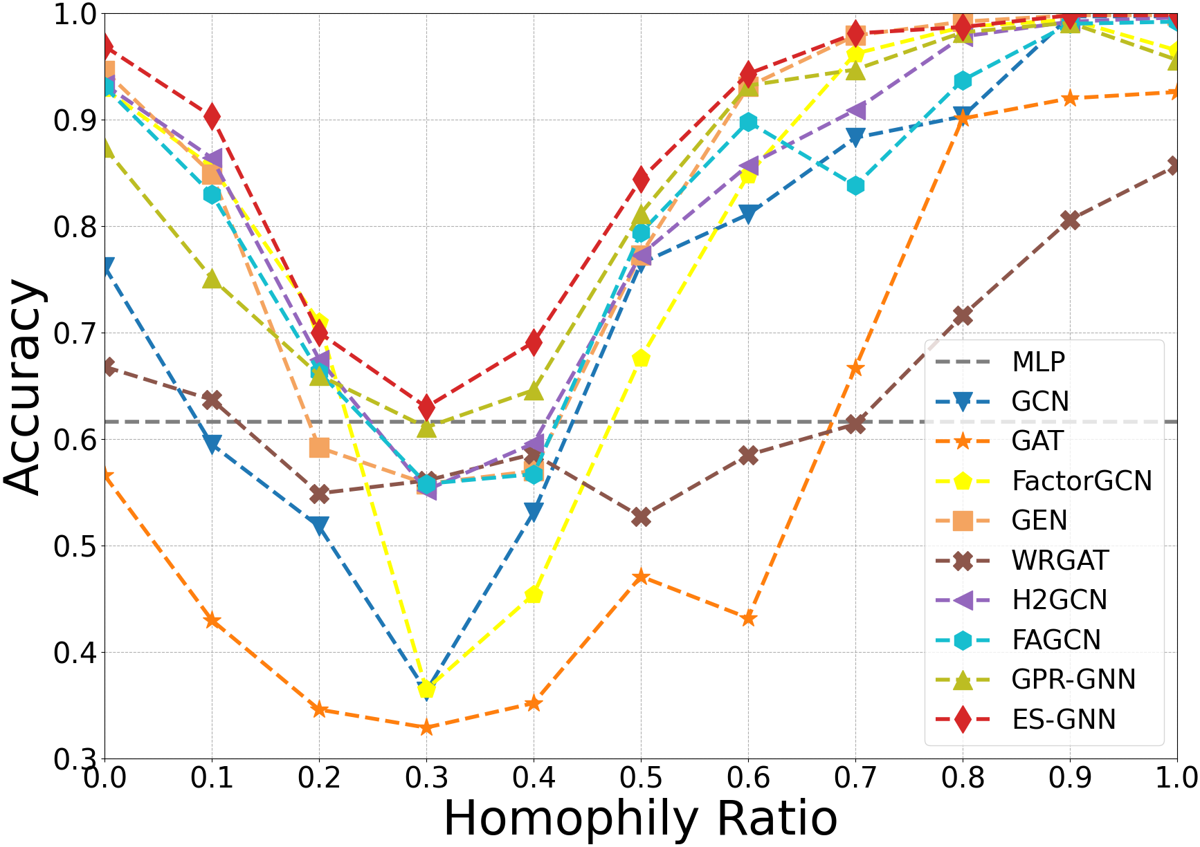
Figure 4: Results of different models on synthetic graphs with varied homophily ratios, where ES-GNN constantly outperform all the baselines including conventional GNNs and the state-of-the-arts explicitly designed for heterophilic graphs.

6.2 Results on Real-World Graphs

Table IV summaries node classification accuracies on real-world datasets in 100 runs with multiple random splits and different model initializations. In general, ES-GNN achieves state-of-the-art performance on all the eleven datasets, and consistently outperforms all the baselines including four popular graph neural network models and five recent state-of-the-arts which explicitly considers heterophily on graphs. Specifically, compared to the second place models, our method achieves significant performance gains by 17.4% and 9.0% separately on the heterophilic graphs Squirrel and Chameleon, and we have the relative error reductions of 2.5%, 2.4%, and 2.2% on Wisconsin, Cornell, and Texas, respectively. For Actor and Twitch-DE, ES-GNN wins by an average margin of 1.3%. We notice that FactorGCN surprisingly has relative good performance on Squirrel and Chameleon datasets. This phenomenon can be explained by its ability on separating channels for learning disentangled graph aspects, which further verifies our speculation in Section 1, i.e., the different types of information are typically mixed and entangled in the node neighborhood under heterophily. However, FactorGCN dose not continue to perform well on other five heterophilic graphs, mainly because it fails to distinguish between the useful and useless (even harmful) channels, and takes the whole parts for classification. For graphs with strong homophily, ES-GNN maintains competitiveness and exhibits averagely 2.3% superiority upon the state-of-the-art models. We will show our ES-GNN could demonstrate remarkable robustness on homophilic graphs in case of perturbation or noisy links in Section 6.6.

TABLE V: Edge Analysis of our ES-GNN on synthetic graphs with various homophily ratios. Removed Het. gives the percentage (%) of heterophilic node connections excluded from the task-relevant topology and disentangled in the task-irrelevant topology. The last two rows give the corresponding node classification accuracies (%) of ES-GNN and its variant while ablating ES-layer.

$\mathcal{H}_{\text{syn}}$	0.1	0.2	0.3	0.4	0.5	0.6	0.7	0.8	0.9	Avg.
Removed Het.	41.9	53.2	60.8	70.4	74.2	80.7	86.7	87.8	89.9	71.7
ES-GNN	90.0	69.6	62.1	69.6	85.4	93.8	98.3	99.2	100.0	85.3
ES-GNN w/o ES	84.6	57.9	53.3	53.8	74.2	81.7	86.3	90.4	96.7	75.4

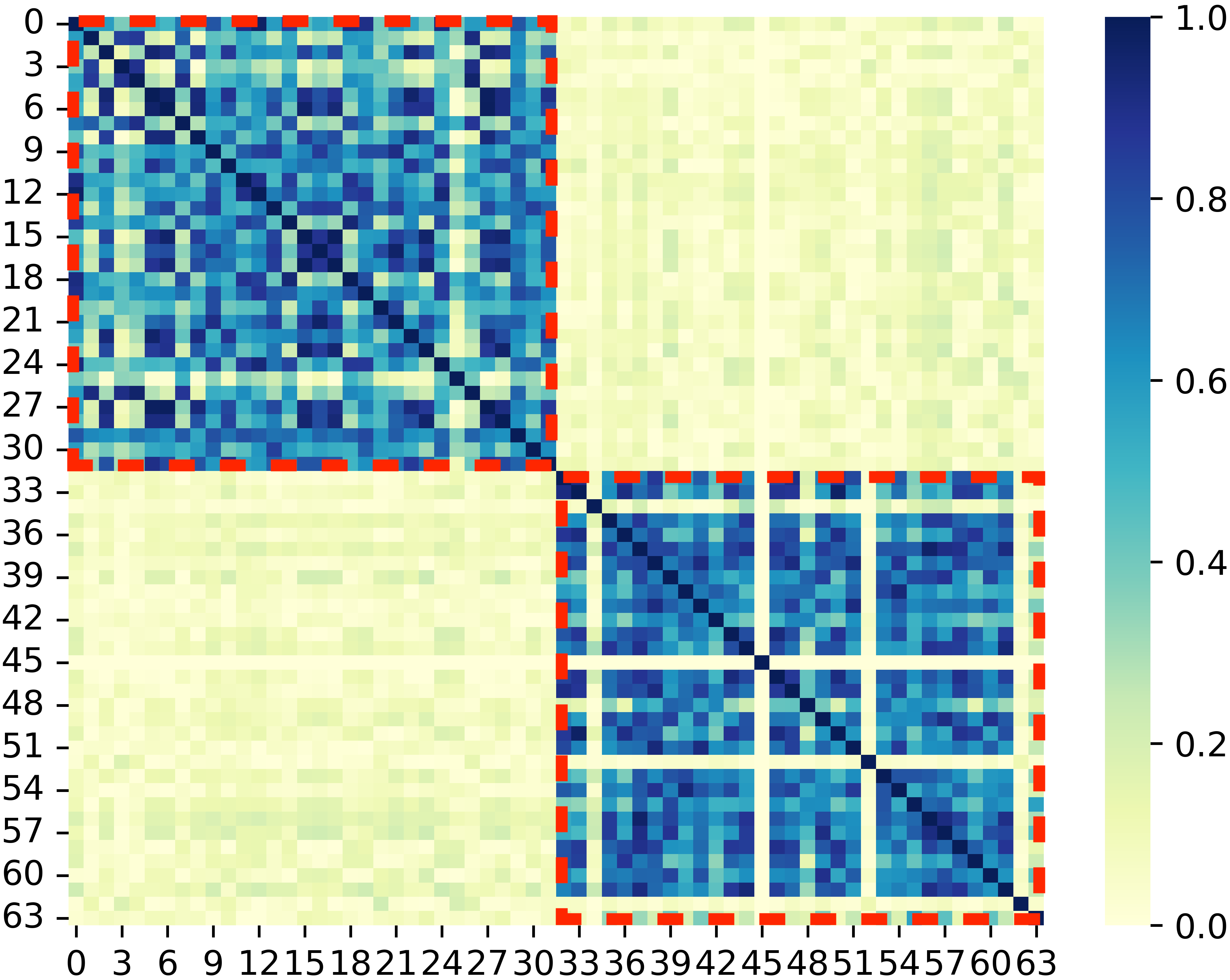
(a) Chameleon

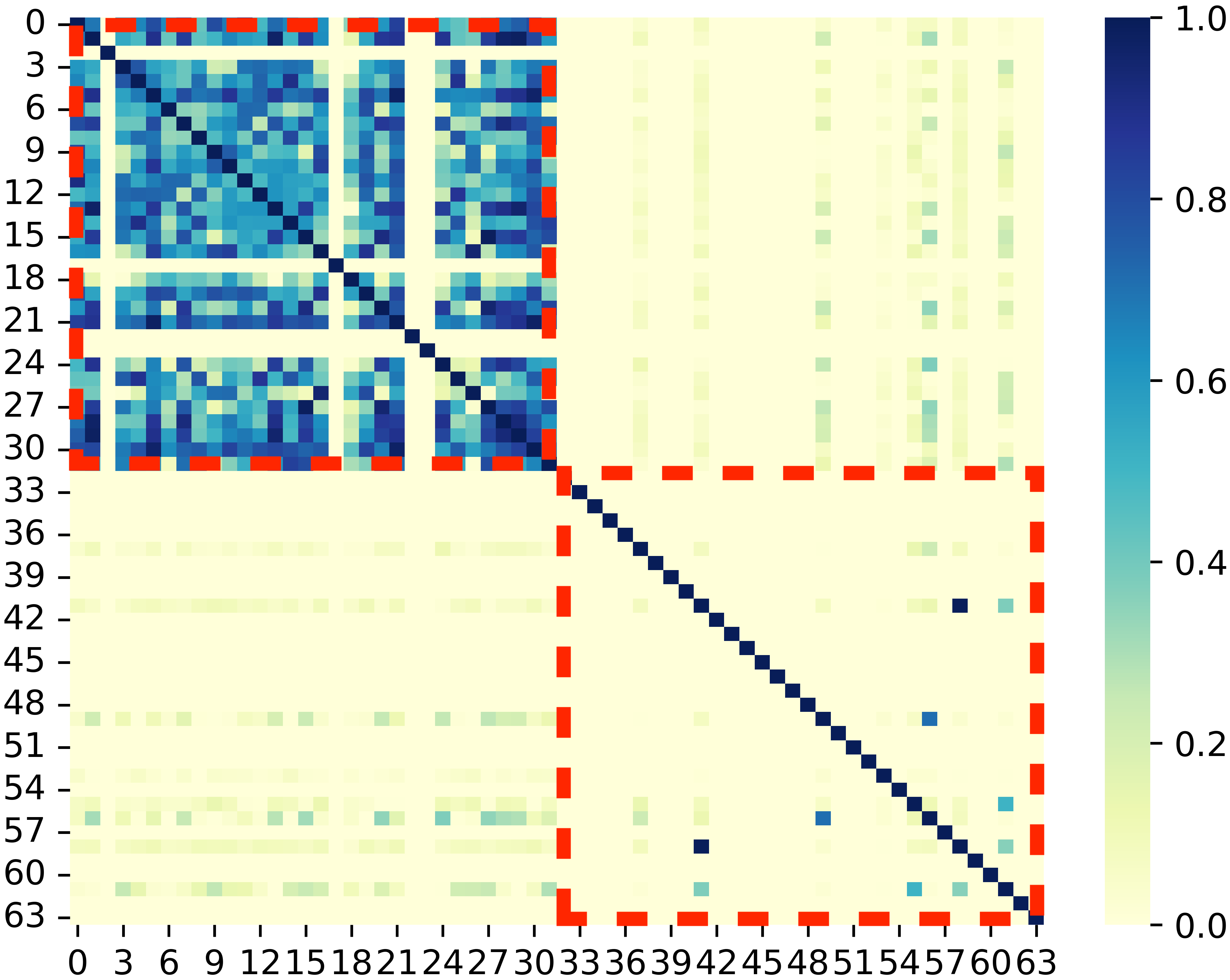
(b) Cora

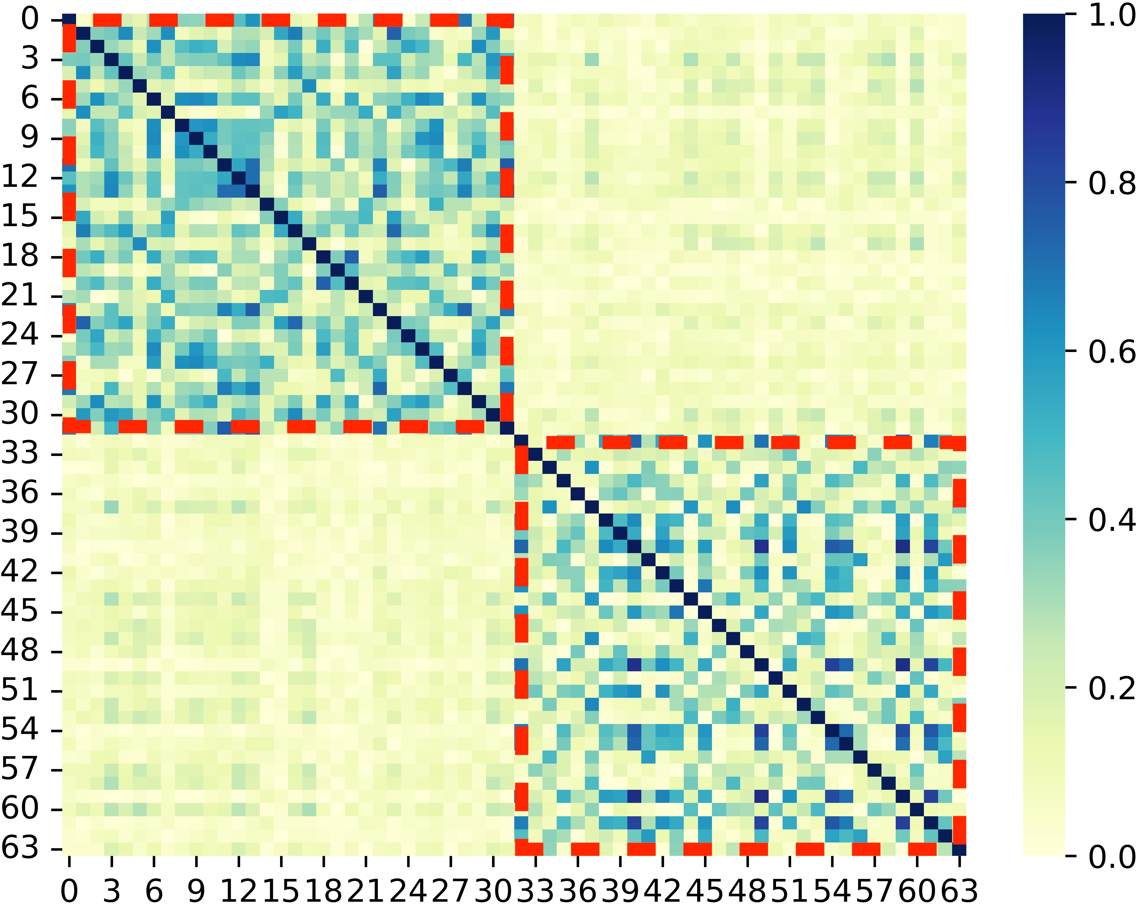
(c) $\mathcal{H}_{\text{syn}}=0.1$

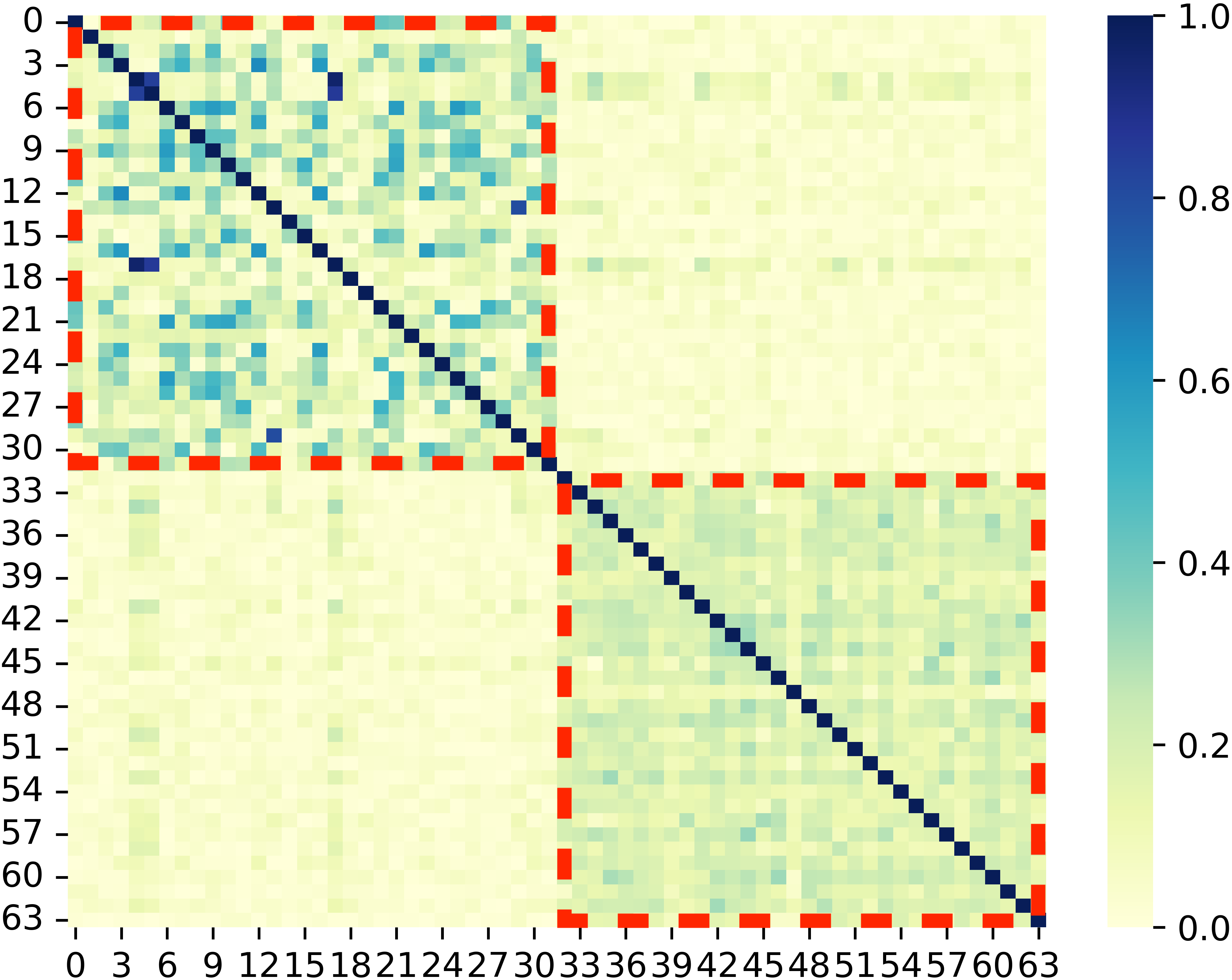
(d) $\mathcal{H}_{\text{syn}}=0.5$

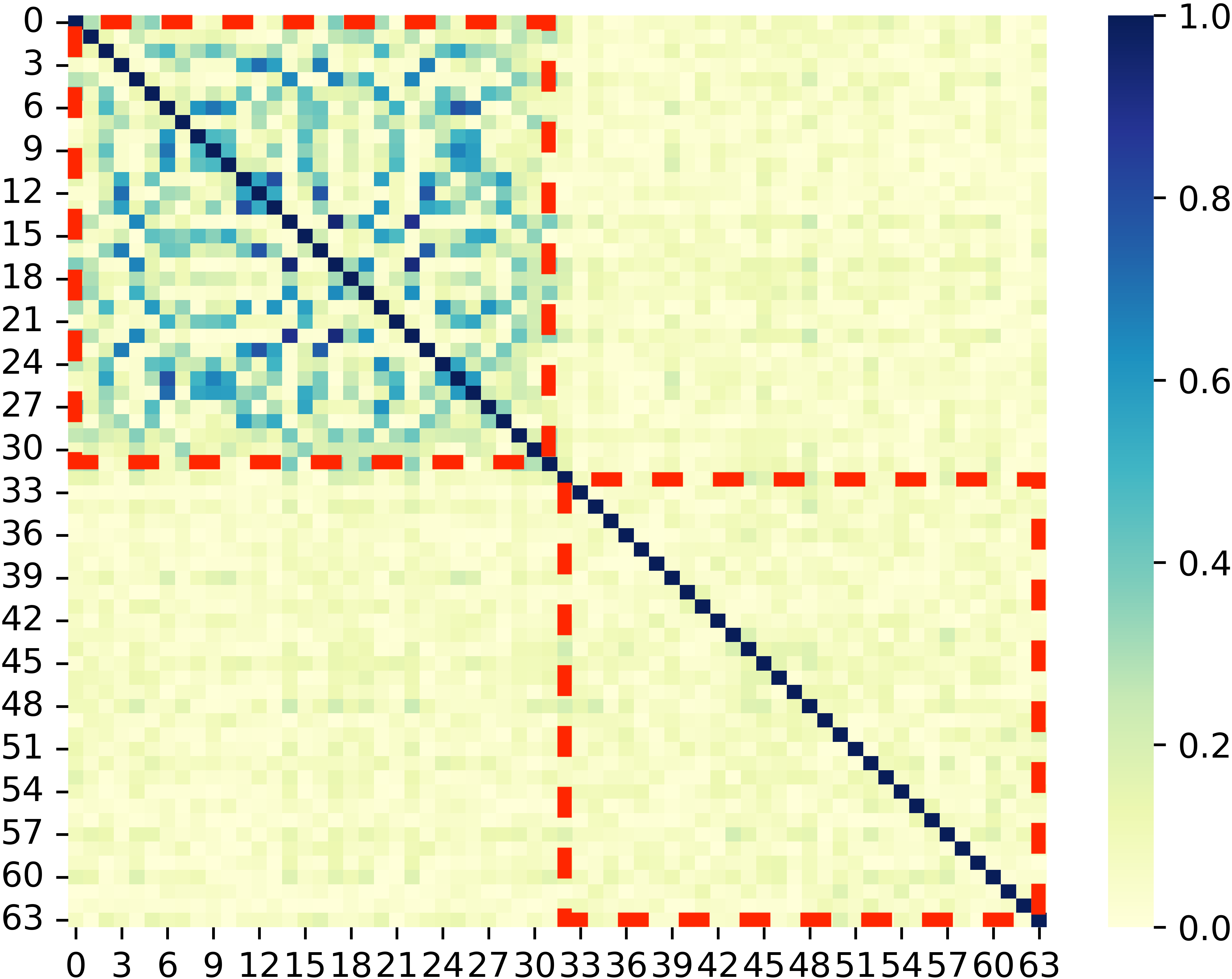
(e) $\mathcal{H}_{\text{syn}}=0.9$

Figure 5: Feature correlation analysis. Two distinct patterns (task-relevant and task-irrelevant topologies) can be learned on Chameleon with $\mathcal{H}=0.23$, while almost all information is retained in the task-relevant channel (0-31) on Cora with $\mathcal{H}=0.81$. On synthetic graphs in (c), (d), and (e), block-wise pattern in the task-irrelevant channel (32-63) is gradually attenuated with the incremental homophily ratios across $0.1$, $0.5$, and $0.9$. ES-GNN presents one general framework which can be adaptive for both heterophilic and homophilic graphs.

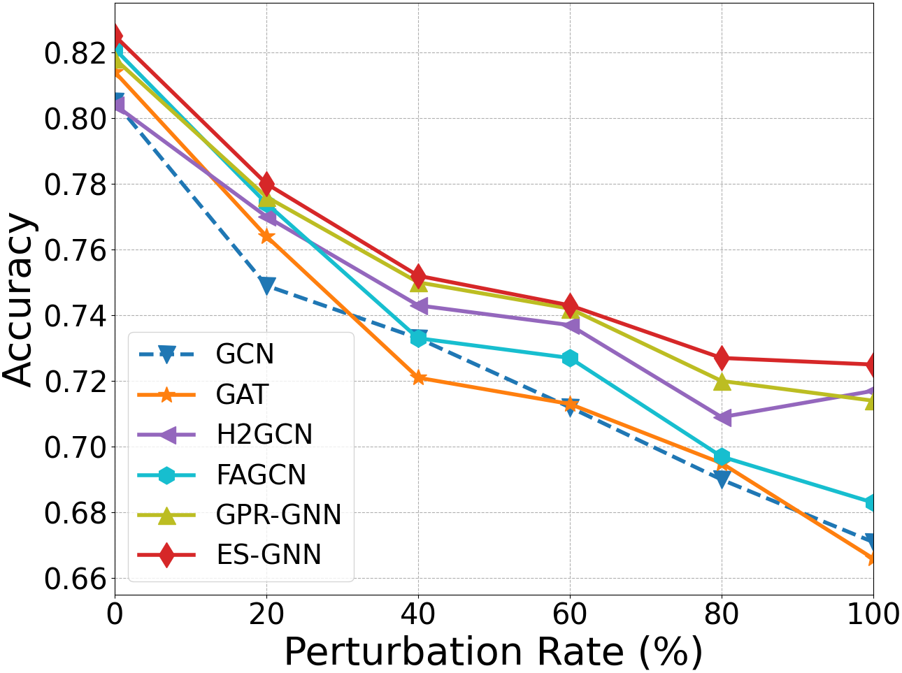
(a) Cora

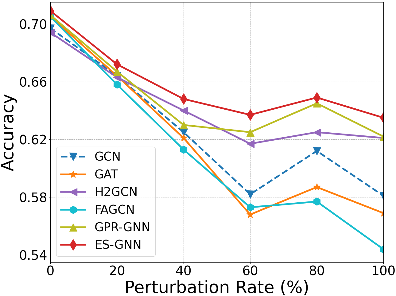
(b) Citeseer

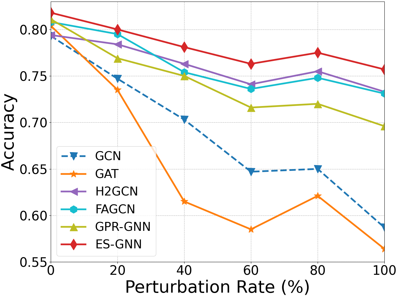
(c) Pubmed

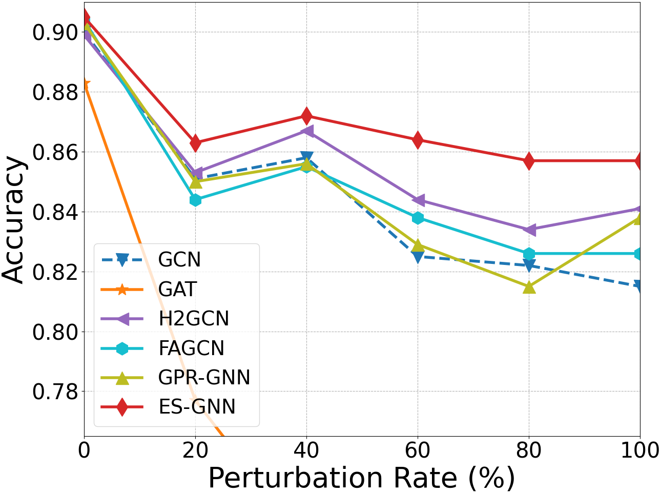
(d) Polblogs

Figure 6: Results of different models on perturbed homophilic graphs. ES-GNN is able to identify the falsely injected (the task-irrelevant) graph edges, and exclude these connections from the final predictive learning, thereby displaying relative robust performance against adversarial edge attacks.

6.3 Results on Synthetic Graphs

We examine the learning ability of various models on graphs across the homophily or heterophily spectrum. From Fig. 4, we have the following observations: (1) Looking through the overall trend, we obtain a “U” pattern on graphs from the lowest to the highest homophily ratios. That suggests GNNs’ prediction performance is not monotonically correlated with graph homophily levels in a strict manner. When it comes to the extreme heterophilic scenario, GNNs tend to alternate node features completely between different classes, thereby still making nodes distinguishable w.r.t. their labels, which coincides with the findings in [63]. (2) Despite the attention mechanism for adaptively utilizing relevant neighborhood information, GAT turns out to be the least robust method to arbitrary graphs. The entangled information in the mixed assortativity and disassortativity provides weak supervision signals for learning the attention weights. FactorGCN employs a graph factorization to disentangle different graph aspects but still adopts all of them for prediction without judgement, thereby performing poorly especially on the tough cases of $\mathcal{H}_{\text{syn}}=0.3,0.4,\text{ and }0.5$. (3) Both FAGCN and GPR-GNN model the dissimilarity between nearby nodes to go beyond the smoothness assumption in conventional GNNs, and display some superiority under heterophily. However, the correlation between graph edges and classification tasks is not explicitly defined and emphasized in their designs. In other words, the classification-harmful information still could be preserved in their node dissimilarity. Experimental results also show that these methods are constantly beaten by our disentangled approach. (4) The proposed ES-GNN consistently outperforms, or matches, others across different graphs with different homophily levels, especially in the hardest case with $\mathcal{H}_{\text{syn}}=0.3$ where some baselines even perform worse than MLP. This is mainly because our ES-GNN is able to distinguish between task-relevant and irrelevant graph links, and makes prediction with the most correlated features only. We further provide detailed analyses in the following sections.

6.4 Edge Analysis

We analyze the split edges from our ES-layer using synthetic graphs as an example in this section. According to Section 6.1.2, the synthetic edges are defined as the task-relevant connections if they link nodes from the same class, and the task-irrelevant ones otherwise. Therefore, we calculate the percentages of heterophilic node connections, which are excluded from our task-relevant topology and disentangled in the task-irrelevant one, so as to investigate the discerning ability of ES-GNN between edges in different types. As can be observed in Table V, 71.7% task-irrelevant edges are identified on average across various homophily ratios. On the other hand, we also report the classification accuracies of ES-GNN and its variant while ablating ES-layer, from which approximately 10% degradation can be observed. All of these strongly validate the effectiveness of our ES-layer and reasonably interprets the good performance of ES-GNN.

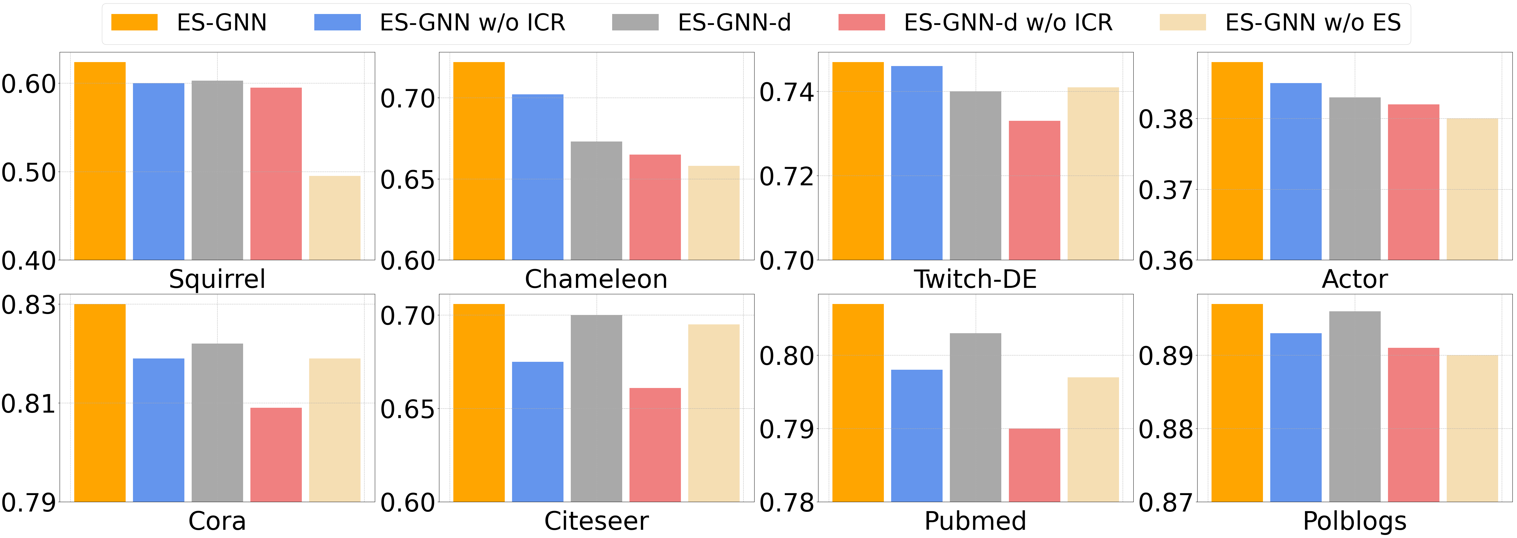
Figure 7: Ablation study of ES-GNN on eight datasets in node classification.

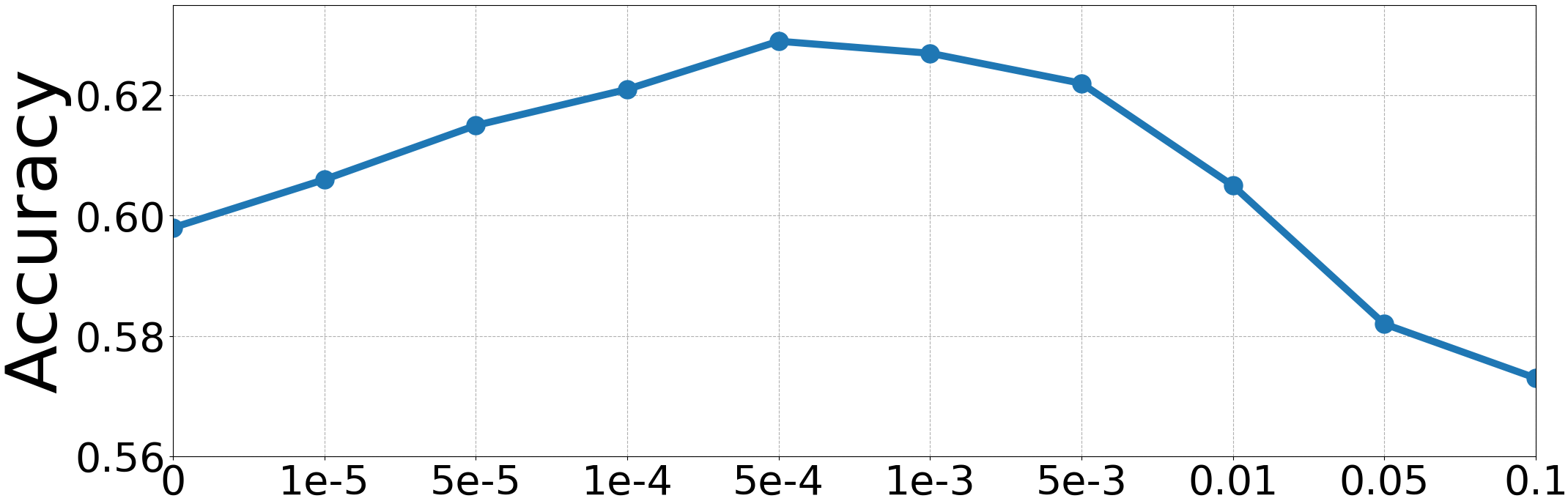
(a) Squirrel

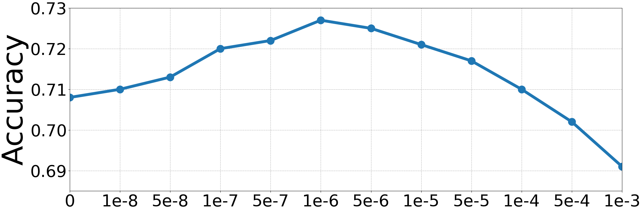
(b) Chameleon

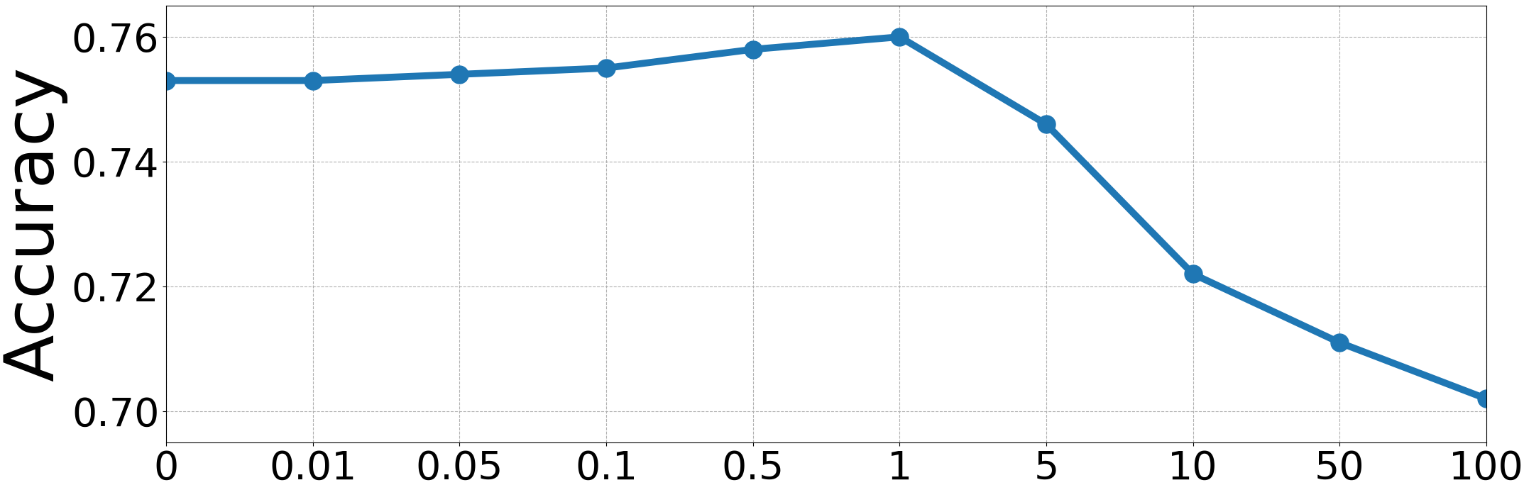
(c) Twitch-DE

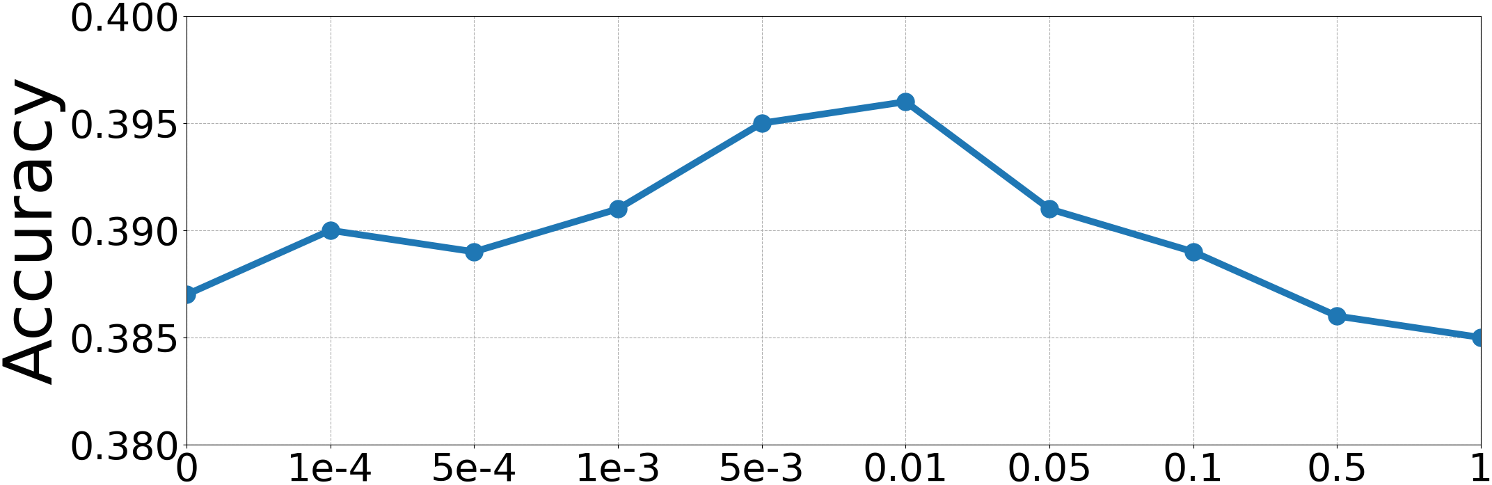
(d) Actor

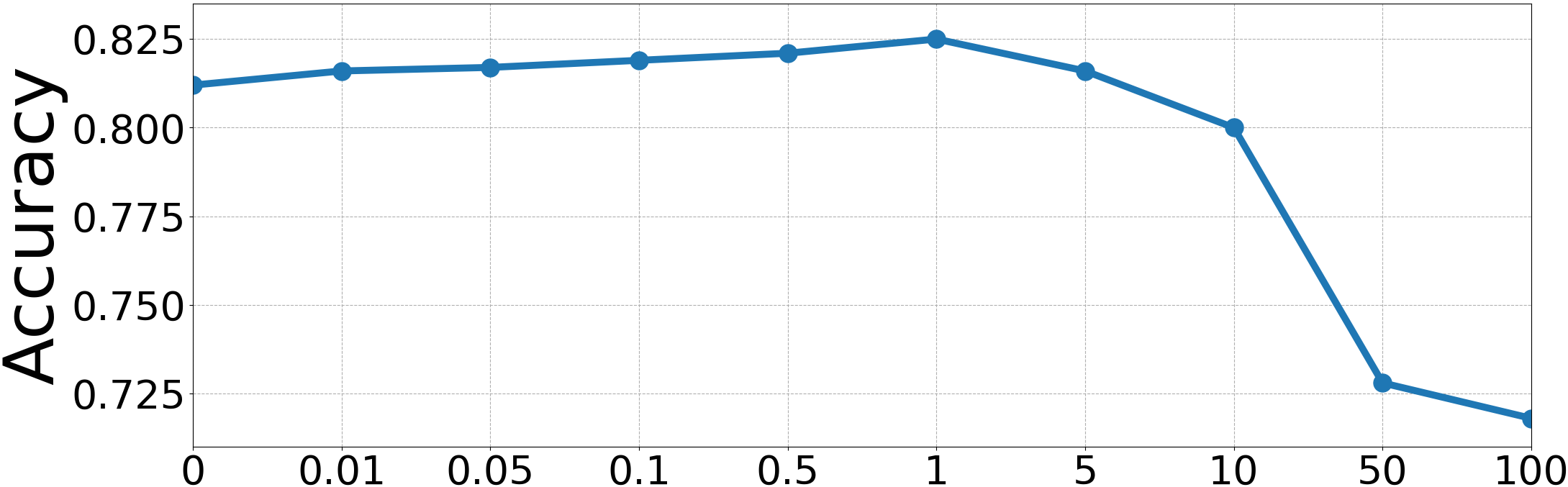
(e) Cora

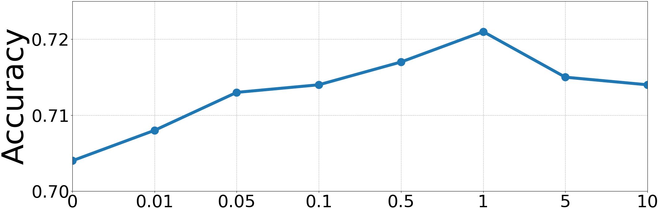
(f) Citeseer

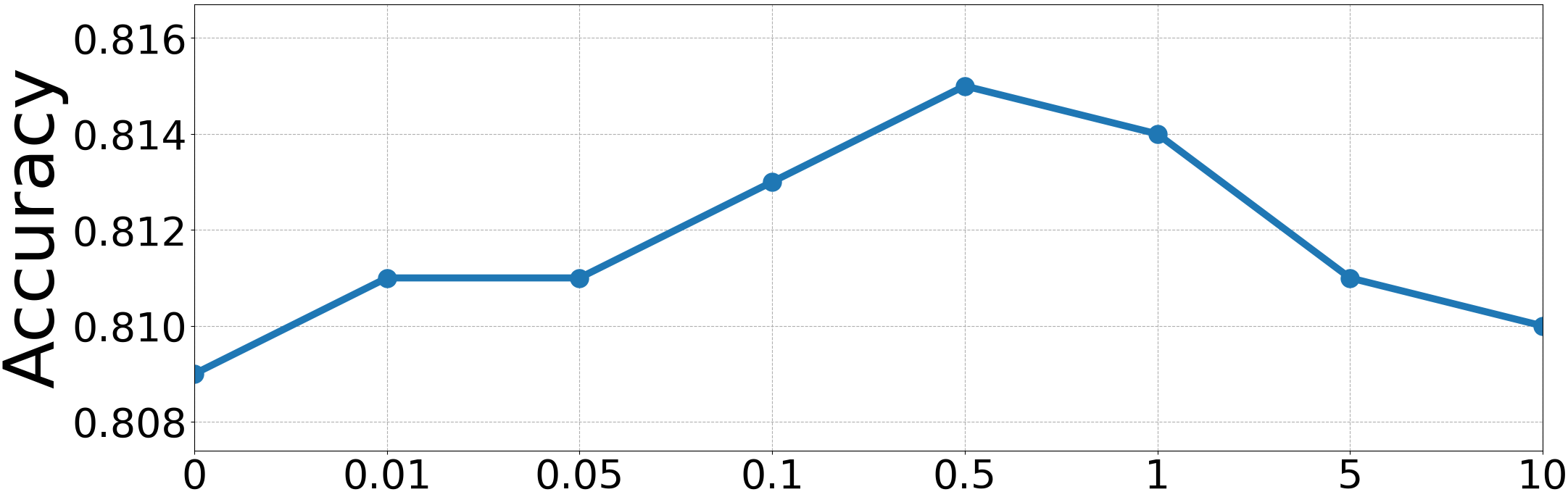
(g) Pubmed

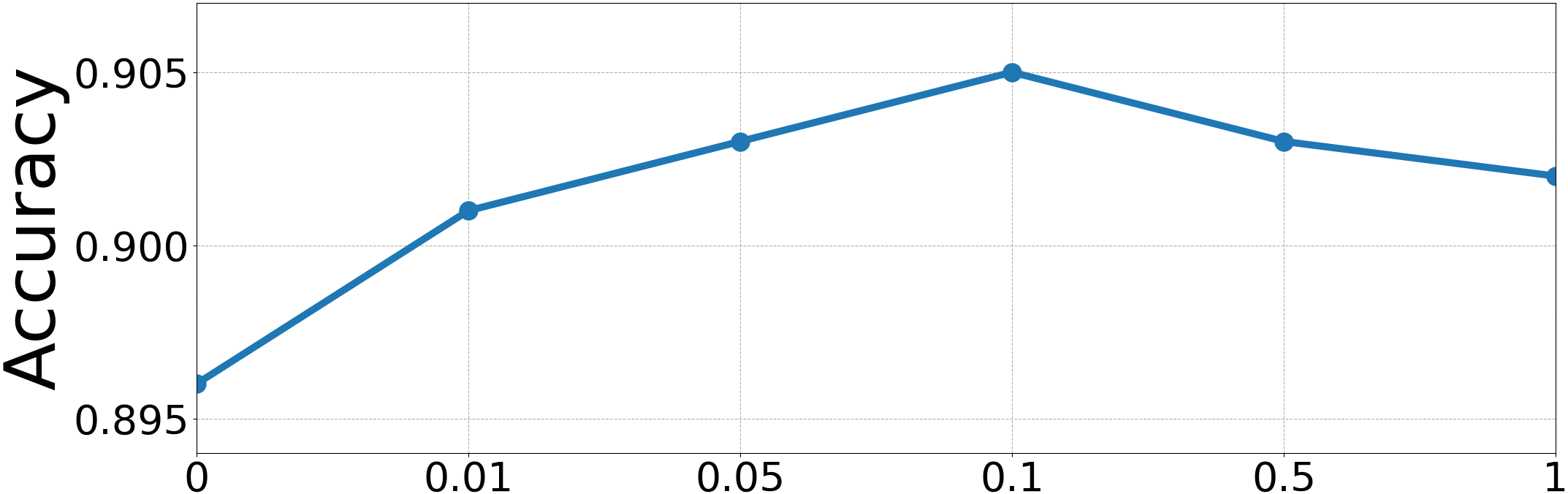
(h) Polblogs

Figure 8: Sensitivity analysis of coefficient $\lambda_{\text{ICR}}$.

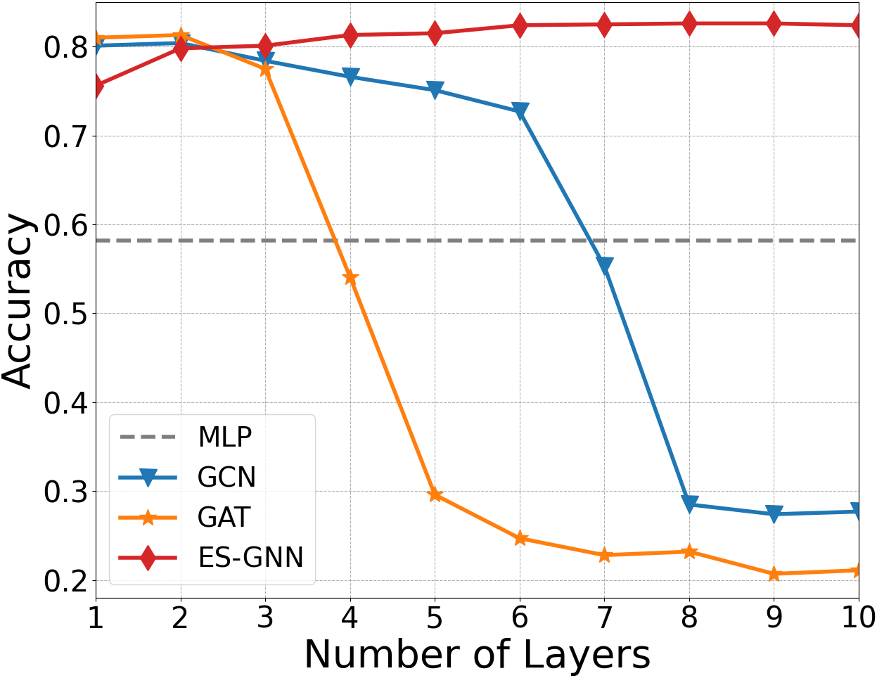
(a) Cora

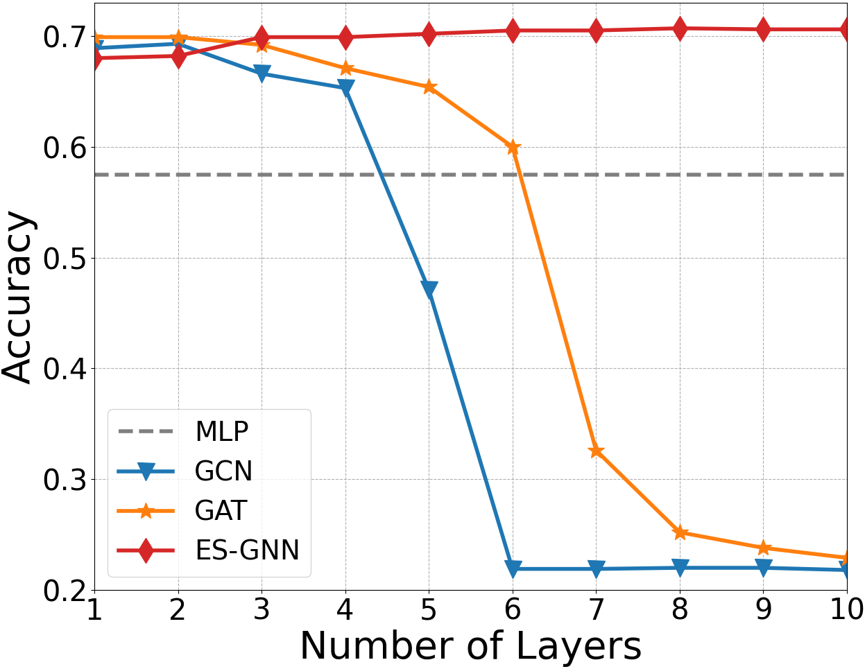
(b) Citeseer

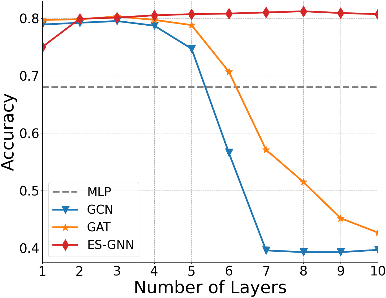
(c) Pubmed

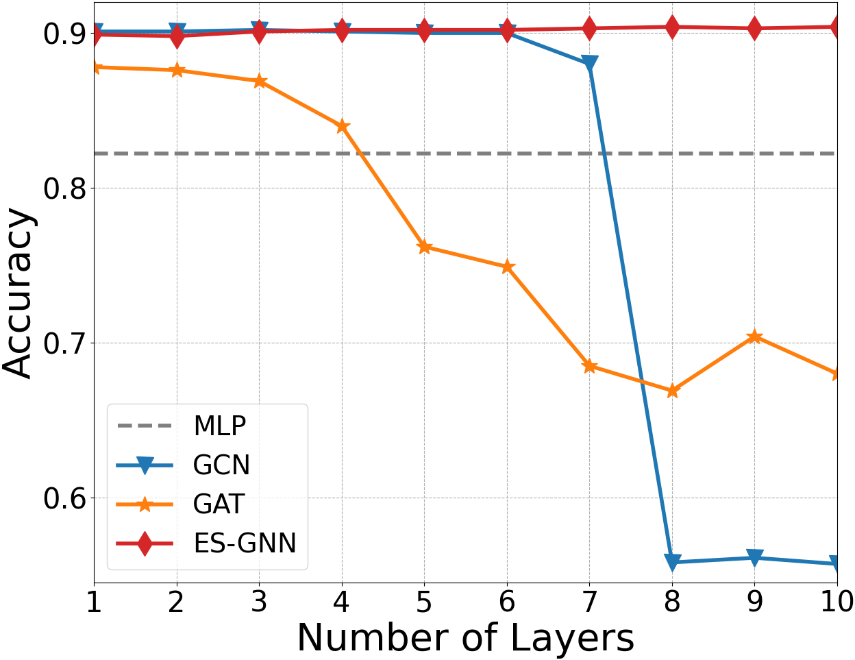
(d) Polblogs

Figure 9: Classification accuracy vs. model depths.

6.5 Correlation Analysis

To better understand our proposed method, we investigate the disentangled features on Chameleon, Cora, and three synthetic graphs as typical examples in Fig. 5. Clearly, on the strong heterophilic graph Chameleon with $\mathcal{H}=0.23$, correlation analysis of learned latent features displays two clear block-wise patterns, each of which represents task-relevant or task-irrelevant aspect respectively. In contrast, on the citation network Cora with $\mathcal{H}=0.81$, the node connections are in line with the classification task, since scientific papers mostly cite or are cited by others in the same research topic. Thus, most information will be retained in the task-relevant topology, while very minor information could be disentangled in the task-irrelevant topology (see Fig. 5b). On the other hand, the results on synthetic graphs from Fig. 5c to 5e display an attenuating trend on the second block-wise pattern with the incremental homophily ratios across $0.1,0.5,\text{ and }0.9$. This correlation analysis empirically verifies that our ES-GNN successfully disentangles the task-relevant and irrelevant features, and also demonstrates its universal adaptivity on different types of networks.

6.6 Robustness Analysis

By splitting the original graph edge set into task-relevant and task-irrelevant subsets, our proposed ES-GNN enjoys strong robustness particularly on homophilic graphs, since perturbed or noisy aspects of nodes could be purified from the task-relevant topology and disentangled in the task-irrelevant topology. To examine this, we randomly inject fake edges into graphs with perturbed rates from 0% to 100% with a step size of 20%. Adversarially perturbed examples are generated from graphs with strong homophily, such as Cora, Citseer, Pubmed, and Polblogs. As shown in Fig. 6, models considering graphs beyond homophily, i.e., H2GCN, FAGCN, GPR-GNN, and our model, consistently display a more robust behavior than GCN and GAT. That is mainly because fake edges may connect nodes across different labels, and consequently cause erroneous information sharing in the conventional methods.

On the other hand, our ES-GNN beats all the state-of-the-arts by an average margin of 2% to 3% on Citeseer, Pubmed, and Polblogs while displaying relatively the same results on Cora. We attribute this to the capability of our model in associating node connections with learning tasks. Take Pubmed dataset as an example. We investigate the learned task-relevant topologies and find that 81.0%, 73.0%, 82.1%, 83.0%, 82.6% fake links get removed on adversatial graphs with perturbation rates from 20% to 100%. This also offers evidences supporting that our ES-layer is able to distinguish between task-relevant and irrelevant node connections. Therefore, despite a large number of false edge injections, the proximity information of nodes can still be reasonably mined in our model to predict their labels. Importantly, these empirical results also indicate that ES-GNN can still identify most of the task-irrelevant edges though no clear similarity or association between the connected nodes exists in the adversarial setting.

6.7 Alleviating Over-smoothing Problem

In order to verify whether ES-GNN alleviates the over-smoothing problem, we compare it with GCN and GAT by varying the layer number in Fig. 9. It can be observed that these two baselines attain their highest results when the number of layers reaches around two. As the layer goes deeper, the accuracies of both GCN and GAT gradually drop to a lower point. On the contrary, our ES-GNN presents a stable curve. In spite of starting from a relative lower point, the performance of ES-GNN keeps improving as the model depths increase, and eventually outperforms both GCN and GAT. The main reason is that, our ES-GNN can adaptively utilize proper graph edges in different layers to attain the task-optimal results with enlarged receptive fields. In other words, once an edge stops passing useful information or starts passing harmful messages, ES-GNN tends to identify it and remove it from learning the task-correlated representations, thereby having the ability of mitigating the over-smoothing problem.

6.8 Channel Analysis and Ablation Study

In this section, we compare ES-GNN with its variant ES-GNN-d which takes dual (both the task-relevant and irrelevant) channels for prediction, and perform an ablation study. Fig. 7 provides comparison on eight real-world datasets as examples. Here, we first specify some annotations including 1) “w/o ICR”: without regularization loss $\mathcal{L}_{\text{ICR}}$, and 2) “w/o ES”: without edge splitting (ES-) layer. Overall, two conclusions can be drawn from Fig. 7. First, ES-GNN is consistently better than ES-GNN-d, implying that the task-irrelevant channels indeed capture some false information where model performance downgrades even with the doubled feature dimensions. Second, removing either ICR or ES-layer from both ES-GNN and ES-GNN-d leads to a clear accuracy drop. That validates the effectiveness of our model designs.

6.9 Sensitivity Analysis of Coefficient $\lambda_{\text{ICR}}$

We test the effect of the irrelevant consistency coefficient $\lambda_{\text{ICR}}$, and plot the learning performance of our model on eight real-world datasets as examples in Fig. 8 by varying $\lambda_{\text{ICR}}$ with different values. For example, the classification accuracy on Squirrel in Fig. 8a goes up first and then gradually drops. Promising results can be attained by choosing $\lambda_{\text{ICR}}$ from $\left[5\mathrm{e}{-5},5\mathrm{e}{-3}\right]$. Similar trends can be also observed on the other datasets, where $\lambda_{\text{ICR}}$ is relatively robust within a wide albeit distinct interval.

7 Conclusion

In this paper, we develop a novel graph learning framework which enables GNNs to go beyond the strong homophily assumption on graphs. We manage to establish correlation between node connections and learning tasks through one plausible hypothesis, based on which ES-GNN is derived with an interpretable edge splitting. Our ES-GNN essentially partitions the original graph structure into the task-relevant and irrelevant topologies as guide to disentangle node features, whereby the classification-harmful information can be disentangled and excluded from the final prediction target.

Theoretical analysis illustrates our motivation and offers interpretations on the expressive power of ES-GNN on different types of networks. To provide empirical verification, we conduct extensive experiments over 11 benchmark and 1 synthetic datasets. The node classification results show that ES-GNN constantly outperforms the other 9 competitive GNNs (including 5 state-of-the-arts explicitly designed for heterophily) on graphs with either homophily or heterophily. In particular, we also conduct analysis on the split edges, correlation among disentangled features, model robustness, and the ablated variants. All of these results demonstrate the success of ES-GNN in identifying graph edges between different types, which also validates the effectiveness of our interpretable edge splitting.

In future work, we will further explore more sophisticated designs in the edge splitting layer. Another interesting direction would be how to extend our learning paradigm in accomplishing graph-level tasks.

Jingwei Guo received the First-class (Hons) degree in Applied Mathematics from University of Liverpool, UK, in 2018. After finishing his undergraduate study, he worked as a Research Associate at Xi’an Jiaotong-Liverpool University of China for a year. He is currently pursing his PhD degree at University of Liverpool, UK. His research focuses on developing new graph neural networks, and applying the techniques in various domains.

Kaizhu Huang (corresponding author) Short Bio: Kaizhu Huang works on machine learning, neural information processing, and pattern recognition. He is currently a tenured Professor of ECE at Duke Kunshan University (DKU). Prof. Huang obtained his PhD degree from Chinese University of Hong Kong (CUHK) in 2004. He worked in Fujitsu Research Centre, CUHK, University of Bristol, National Laboratory of Pattern Recognition, Chinese Academy of Sciences, and Xi’an Jiaotong-Liverpool University from 2004 to 2022. Prof. Huang has been working in machine learning, neural information processing, and pattern recognition. He was the recipient of 2011 Asia Pacific Neural Network Society Young Researcher Award. He received best paper or book award five times and published extensively in journals (JMLR, Neural Computation, IEEE T-PAMI, IEEE T-NNLS, IEEE T-BME, IEEE T-Cybernetics) and conferences (NeurIPS, IJCAI, SIGIR, UAI, CIKM, ICDM, ICML, ECML, CVPR). He serves as associated editors/advisory board members in a number of journals and book series. He was invited as keynote speaker in more than 30 international conferences or workshops.

Rui Zhang received the First-class (Hons) degree in Telecommunication Engineering from Jilin University of China in 2001 and the Ph.D. degree in Computer Science and Mathematics from University of Ulster, UK in 2007. After finishing her PhD study, she worked as a Research Associate at University of Bradford and University of Bristol in the UK for 5 years. She joined Xi’an Jiaotong-Liverpool University in 2012 and currently holds the position of Associate Professor. Her research interests include machine learning, data mining and statistical analysis.

Xinping Yi received the Ph.D. degree in electronics and communications from Télécom ParisTech, Paris, France, in 2015. He is currently a Lecturer (Assistant Professor) with the Department of Electrical Engineering and Electronics, University of Liverpool, U.K. Prior to Liverpool, he was a Research Associate with Technische Universität Berlin, Berlin, Germany, from 2014 to 2017, a Research Assistant with EURECOM, Sophia Antipolis, France, from 2011 to 2014, and a Research Engineer with Huawei Technologies, Shenzhen, China, from 2009 to 2011. His main research interests include information theory, graph theory, and machine learning, and their applications in wireless communications and artificial intelligence.

References

- [1] G. Ciano, A. Rossi, M. Bianchini, and F. Scarselli, “On inductive–transductive learning with graph neural networks,” IEEE Transactions on Pattern Analysis and Machine Intelligence, vol. 44, no. 2, pp. 758–769, 2021.
- [2] J. Zhou, G. Cui, S. Hu, Z. Zhang, C. Yang, Z. Liu, L. Wang, C. Li, and M. Sun, “Graph neural networks: A review of methods and applications,” AI Open, vol. 1, pp. 57–81, 2020.
- [3] T. Chen and R. C.-W. Wong, “Handling information loss of graph neural networks for session-based recommendation,” in Proceedings of the 26th ACM SIGKDD International Conference on Knowledge Discovery & Data Mining, 2020, pp. 1172–1180.
- [4] Z. Zhang, P. Cui, and W. Zhu, “Deep learning on graphs: A survey,” IEEE Transactions on Knowledge and Data Engineering, 2020.
- [5] J. Gilmer, S. S. Schoenholz, P. F. Riley, O. Vinyals, and G. E. Dahl, “Neural message passing for quantum chemistry,” in International Conference on Machine Learning. PMLR, 2017, pp. 1263–1272.
- [6] F. Wu, A. Souza, T. Zhang, C. Fifty, T. Yu, and K. Weinberger, “Simplifying graph convolutional networks,” in International Conference on Machine Learning. PMLR, 2019, pp. 6861–6871.
- [7] M. Balcilar, G. Renton, P. Héroux, B. Gaüzère, S. Adam, and P. Honeine, “Analyzing the expressive power of graph neural networks in a spectral perspective,” in International Conference on Learning Representations, 2020.
- [8] Y. Ma, X. Liu, T. Zhao, Y. Liu, J. Tang, and N. Shah, “A unified view on graph neural networks as graph signal denoising,” in Proceedings of the 30th ACM International Conference on Information & Knowledge Management, 2021, pp. 1202–1211.
- [9] M. Zhu, X. Wang, C. Shi, H. Ji, and P. Cui, “Interpreting and unifying graph neural networks with an optimization framework,” in Proceedings of the Web Conference 2021, 2021, pp. 1215–1226.
- [10] J. Zhu, Y. Yan, L. Zhao, M. Heimann, L. Akoglu, and D. Koutra, “Beyond homophily in graph neural networks: current limitations and effective designs,” Advances in Neural Information Processing Systems, vol. 33, 2020.
- [11] E. Chien, J. Peng, P. Li, and O. Milenkovic, “Adaptive universal generalized pagerank graph neural network,” in International Conference on Learning Representations, 2021. [Online]. Available: https://openreview.net/forum?id=n6jl7fLxrP
- [12] J. Zhu, R. A. Rossi, A. Rao, T. Mai, N. Lipka, N. K. Ahmed, and D. Koutra, “Graph neural networks with heterophily,” in Proceedings of the AAAI Conference on Artificial Intelligence, vol. 35, no. 12, 2021, pp. 11 168–11 176.
- [13] R. Wang, S. Mou, X. Wang, W. Xiao, Q. Ju, C. Shi, and X. Xie, “Graph structure estimation neural networks,” in Proceedings of the Web Conference 2021, 2021, pp. 342–353.
- [14] S. Suresh, V. Budde, J. Neville, P. Li, and J. Ma, “Breaking the limit of graph neural networks by improving the assortativity of graphs with local mixing patterns,” Proceedings of the 27th ACM SIGKDD Conference on Knowledge Discovery & Data Mining, 2021.
- [15] L. Yang, W. Zhou, W. Peng, B. Niu, J. Gu, C. Wang, X. Cao, and D. He, “Graph neural networks beyond compromise between attribute and topology,” in Proceedings of the ACM Web Conference 2022, 2022, pp. 1127–1135.
- [16] H. Nt and T. Maehara, “Revisiting graph neural networks: All we have is low-pass filters,” arXiv preprint arXiv:1905.09550, 2019.
- [17] M. McPherson, L. Smith-Lovin, and J. M. Cook, “Birds of a feather: Homophily in social networks,” Annual review of sociology, vol. 27, no. 1, pp. 415–444, 2001.
- [18] D. Bo, X. Wang, C. Shi, and H. Shen, “Beyond low-frequency information in graph convolutional networks,” in AAAI. AAAI Press, 2021.
- [19] M. Liu, Z. Wang, and S. Ji, “Non-local graph neural networks,” IEEE Transactions on Pattern Analysis and Machine Intelligence, 2021.
- [20] Y. Yan, M. Hashemi, K. Swersky, Y. Yang, and D. Koutra, “Two sides of the same coin: Heterophily and oversmoothing in graph convolutional neural networks,” arXiv preprint arXiv:2102.06462, 2021.
- [21] Z. Fang, L. Xu, G. Song, Q. Long, and Y. Zhang, “Polarized graph neural networks,” in Proceedings of the ACM Web Conference 2022, 2022, pp. 1404–1413.
- [22] X. Li, R. Zhu, Y. Cheng, C. Shan, S. Luo, D. Li, and W. Qian, “Finding global homophily in graph neural networks when meeting heterophily,” arXiv preprint arXiv:2205.07308, 2022.
- [23] K. Oono and T. Suzuki, “Graph neural networks exponentially lose expressive power for node classification,” in International Conference on Learning Representations, 2020. [Online]. Available: https://openreview.net/forum?id=S1ldO2EFPr
- [24] P. Veličković, G. Cucurull, A. Casanova, A. Romero, P. Liò, and Y. Bengio, “Graph attention networks,” International Conference on Learning Representations, 2018, accepted as poster. [Online]. Available: https://openreview.net/forum?id=rJXMpikCZ
- [25] D. Kim and A. Oh, “How to find your friendly neighborhood: Graph attention design with self-supervision,” in International Conference on Learning Representations, 2021. [Online]. Available: https://openreview.net/forum?id=Wi5KUNlqWty
- [26] P. Sen, G. Namata, M. Bilgic, L. Getoor, B. Gallagher, and T. Eliassi-Rad, “Collective classification in network data,” AI Mag., vol. 29, pp. 93–106, 2008.
- [27] B. Rozemberczki, C. Allen, and R. Sarkar, “Multi-scale attributed node embedding,” Journal of Complex Networks, vol. 9, no. 2, p. cnab014, 2021.
- [28] D. Lim, X. Li, F. Hohne, and S.-N. Lim, “New benchmarks for learning on non-homophilous graphs,” arXiv preprint arXiv:2104.01404, 2021.
- [29] L. A. Adamic and N. Glance, “The political blogosphere and the 2004 us election: Divided they blog,” in Proceedings of the 3rd international workshop on Link discovery, 2005, pp. 36–43.
- [30] W. Jin, Y. Ma, X. Liu, X. Tang, S. Wang, and J. Tang, “Graph structure learning for robust graph neural networks,” in Proceedings of the 26th ACM SIGKDD International Conference on Knowledge Discovery & Data Mining, 2020, pp. 66–74.
- [31] H. Pei, B. Wei, K. C.-C. Chang, Y. Lei, and B. Yang, “Geom-gcn: Geometric graph convolutional networks,” ArXiv, vol. abs/2002.05287, 2020.
- [32] J. Tang, J. Sun, C. Wang, and Z. Yang, “Social influence analysis in large-scale networks,” in Proceedings of the 15th ACM SIGKDD international conference on Knowledge discovery and data mining, 2009, pp. 807–816.
- [33] T. N. Kipf and M. Welling, “Semi-supervised classification with graph convolutional networks,” in International Conference on Learning Representations (ICLR), 2017.
- [34] K. Xu, C. Li, Y. Tian, T. Sonobe, K.-i. Kawarabayashi, and S. Jegelka, “Representation learning on graphs with jumping knowledge networks,” in International Conference on Machine Learning. PMLR, 2018, pp. 5453–5462.
- [35] Y. Yang, Z. Feng, M. Song, and X. Wang, “Factorizable graph convolutional networks,” Advances in Neural Information Processing Systems, vol. 33, 2020.
- [36] K.-H. Lai, D. Zha, K. Zhou, and X. Hu, “Policy-gnn: Aggregation optimization for graph neural networks,” in Proceedings of the 26th ACM SIGKDD International Conference on Knowledge Discovery & Data Mining (KDD), 2020, pp. 461–471.
- [37] E. Isufi, F. Gama, and A. Ribeiro, “Edgenets: Edge varying graph neural networks,” IEEE Transactions on Pattern Analysis and Machine Intelligence, 2021.
- [38] F. M. Bianchi, D. Grattarola, L. Livi, and C. Alippi, “Graph neural networks with convolutional arma filters,” IEEE Transactions on Pattern Analysis and Machine Intelligence, 2021.
- [39] Y. Gao, Y. Feng, S. Ji, and R. Ji, “Hgnn+: General hypergraph neural networks,” IEEE Transactions on Pattern Analysis and Machine Intelligence, vol. 45, no. 3, pp. 3181–3199, 2022.
- [40] G. Bouritsas, F. Frasca, S. P. Zafeiriou, and M. Bronstein, “Improving graph neural network expressivity via subgraph isomorphism counting,” IEEE Transactions on Pattern Analysis and Machine Intelligence, 2022.
- [41] M. Balcilar, P. Héroux, B. Gauzere, P. Vasseur, S. Adam, and P. Honeine, “Breaking the limits of message passing graph neural networks,” in International Conference on Machine Learning. PMLR, 2021, pp. 599–608.
- [42] L. Faber, A. K. Moghaddam, and R. Wattenhofer, “When comparing to ground truth is wrong: On evaluating gnn explanation methods,” in Proceedings of the 27th ACM SIGKDD Conference on Knowledge Discovery & Data Mining, 2021, pp. 332–341.
- [43] X. Wang, Y. Wu, A. Zhang, F. Feng, X. He, and T.-S. Chua, “Reinforced causal explainer for graph neural networks,” IEEE Transactions on Pattern Analysis and Machine Intelligence, 2022.
- [44] T. Schnake, O. Eberle, J. Lederer, S. Nakajima, K. T. Schutt, K.-R. Muller, and G. Montavon, “Higher-order explanations of graph neural networks via relevant walks.” IEEE transactions on pattern analysis and machine intelligence, vol. PP, 2021.
- [45] Y. Min, F. Wenkel, and G. Wolf, “Scattering gcn: Overcoming oversmoothness in graph convolutional networks,” Advances in Neural Information Processing Systems, vol. 33, pp. 14 498–14 508, 2020.
- [46] J. Klicpera, A. Bojchevski, and S. Günnemann, “Predict then propagate: Graph neural networks meet personalized pagerank,” in ICLR, 2019.
- [47] M. Chen, Z. Wei, Z. Huang, B. Ding, and Y. Li, “Simple and deep graph convolutional networks,” in International Conference on Machine Learning. PMLR, 2020, pp. 1725–1735.
- [48] Y. Hou, J. Zhang, J. Cheng, K. Ma, R. T. Ma, H. Chen, and M.-C. Yang, “Measuring and improving the use of graph information in graph neural networks,” in International Conference on Learning Representations (ICLR), 2019.
- [49] Y. Bengio, A. Courville, and P. Vincent, “Representation learning: A review and new perspectives,” IEEE transactions on pattern analysis and machine intelligence, vol. 35, no. 8, pp. 1798–1828, 2013.
- [50] I. Higgins, D. Amos, D. Pfau, S. Racaniere, L. Matthey, D. Rezende, and A. Lerchner, “Towards a definition of disentangled representations,” arXiv preprint arXiv:1812.02230, 2018.
- [51] R. Lopez, J. Regier, M. I. Jordan, and N. Yosef, “Information constraints on auto-encoding variational bayes,” Advances in neural information processing systems, vol. 31, 2018.
- [52] L. Ma, Q. Sun, S. Georgoulis, L. Van Gool, B. Schiele, and M. Fritz, “Disentangled person image generation,” in Proceedings of the IEEE Conference on Computer Vision and Pattern Recognition, 2018, pp. 99–108.
- [53] Z. Zhang, L. Tran, F. Liu, and X. Liu, “On learning disentangled representations for gait recognition,” IEEE Transactions on Pattern Analysis and Machine Intelligence, 2020.
- [54] C. Eom, W. Lee, G. Lee, and B. Ham, “Is-gan: Learning disentangled representation for robust person re-identification,” IEEE transactions on pattern analysis and machine intelligence, 2021.
- [55] J. Ma, P. Cui, K. Kuang, X. Wang, and W. Zhu, “Disentangled graph convolutional networks,” in International conference on machine learning. PMLR, 2019, pp. 4212–4221.
- [56] Y. Liu, X. Wang, S. Wu, and Z. Xiao, “Independence promoted graph disentangled networks,” in Proceedings of the AAAI Conference on Artificial Intelligence, vol. 34, no. 04, 2020, pp. 4916–4923.
- [57] H. Li, X. Wang, Z. Zhang, Z. Yuan, H. Li, and W. Zhu, “Disentangled contrastive learning on graphs,” Advances in Neural Information Processing Systems, vol. 34, pp. 21 872–21 884, 2021.
- [58] E. Jang, S. Gu, and B. Poole, “Categorical reparameterization with gumbel-softmax,” arXiv preprint arXiv:1611.01144, 2016.
- [59] C. J. Maddison, A. Mnih, and Y. W. Teh, “The concrete distribution: A continuous relaxation of discrete random variables,” arXiv preprint arXiv:1611.00712, 2016.
- [60] O. Stretcu, K. Viswanathan, D. Movshovitz-Attias, E. A. Platanios, S. Ravi, and A. Tomkins, “Graph agreement models for semi-supervised learning,” in NeurIPS, 2019.
- [61] D. P. Kingma and J. Ba, “Adam: A method for stochastic optimization,” arXiv preprint arXiv:1412.6980, 2014.
- [62] T. Akiba, S. Sano, T. Yanase, T. Ohta, and M. Koyama, “Optuna: A next-generation hyperparameter optimization framework,” in Proceedings of the 25th ACM SIGKDD international conference on knowledge discovery & data mining, 2019, pp. 2623–2631.
- [63] Y. Ma, X. Liu, N. Shah, and J. Tang, “Is homophily a necessity for graph neural networks?” ArXiv, vol. abs/2106.06134, 2021.