FedAvg with Fine Tuning: Local Updates Lead to Representation Learning
Abstract
The Federated Averaging (FedAvg) algorithm, which consists of alternating between a few local stochastic gradient updates at client nodes, followed by a model averaging update at the server, is perhaps the most commonly used method in Federated Learning. Notwithstanding its simplicity, several empirical studies have illustrated that the output model of FedAvg, after a few fine-tuning steps, leads to a model that generalizes well to new unseen tasks. This surprising performance of such a simple method, however, is not fully understood from a theoretical point of view. In this paper, we formally investigate this phenomenon in the multi-task linear representation setting. We show that the reason behind generalizability of the FedAvg’s output is its power in learning the common data representation among the clients’ tasks, by leveraging the diversity among client data distributions via local updates. We formally establish the iteration complexity required by the clients for proving such result in the setting where the underlying shared representation is a linear map. To the best of our knowledge, this is the first such result for any setting. We also provide empirical evidence demonstrating FedAvg’s representation learning ability in federated image classification with heterogeneous data.
1 Introduction
Federated Learning (FL) [36] provides a communication-efficient and privacy preserving means to learn from data distributed across clients such as cell phones, autonomous vehicles, and hospitals. FL aims for each client to benefit from collaborating in the learning process without sacrificing data privacy or paying a substantial communication cost. Federated Averaging (FedAvg) [36] is the predominant FL algorithm. In FedAvg, also known as Local SGD [48, 49, 58], the clients achieve communication efficiency by making multiple local updates of a shared global model before sending the result to the server, which averages the locally updated models to compute the next global model.
FedAvg is motivated by settings with homogeneous data across clients, since multiple local updates should improve model performance on all other clients’ data when their data is similar. In contrast, FedAvg faces two major challenges in more realistic heterogeneous data settings: learning a single global model may not necessarily yield good performance for each individual client, and, multiple local updates may cause the FedAvg updates to drift away from solutions of the global objective [23, 34, 42, 4, 59]. Despite these challenges, several empirical studies [67, 44, 29] have observed that this shared global model trained by FedAvg with several local updates per round when further fine-tuned for individual clients is surprisingly effective in heterogeneous FL settings. These studies motivate us to explore the impact of local updates on post-fine-tuning performance.
Meanwhile, a large number of recent works have shown that representation learning is a powerful paradigm for attaining high performance in multi-task settings, including FL. This is because the tasks’ data often share a small set of features which are useful for downstream tasks, even if the datasets as a whole are heterogeneous. Consider, for example, heterogeneous federated image classification in which each client (task) may have images of different types of animals. It is safe to assume the images share a small number of features, such as body shape and color, which admit a simple and accurate mapping from feature space to label space. Since the number of important features is much smaller than the dimension of the data, knowing these features greatly simplifies each client’s task.
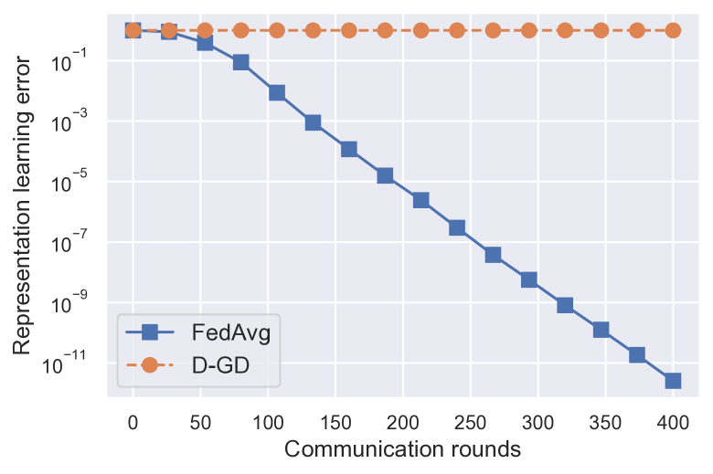
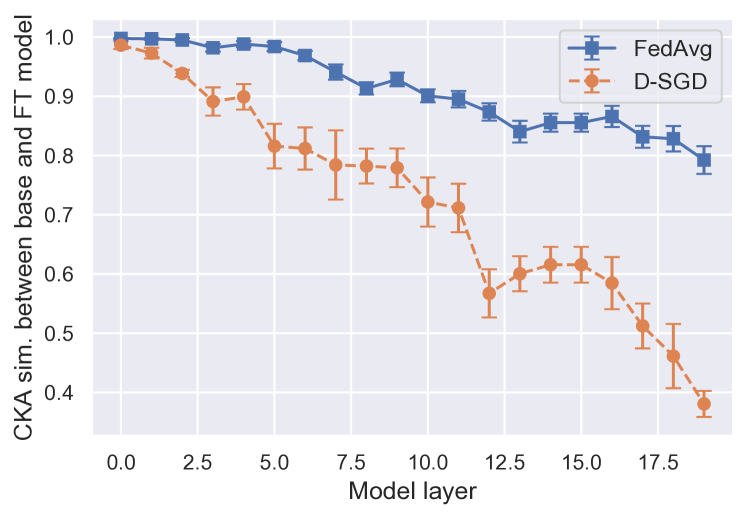
To explore the connection between local updates and representation learning, we first study multi-task linear regression sharing a common ground-truth representation (Figure 2). We observe that FedAvg converges (exponentially fast) to the ground-truth representation in principal angle distance, while Distributed-GD (D-GD), which is effectively FedAvg with one local gradient update, fails to learn the shared representation. A similar concept can be shown in the nonlinear setting. We study a multi-layer CNN on a heterogeneous partition of CIFAR-100 (Figure 2). Since there is not necessarily a ground-truth model here, we evaluate representation learning as follows. We first train the models with FedAvg and Distributed-SGD (D-SGD) then fine-tune the pre-trained models on clients from a new dataset, CIFAR-10. Finally we evaluate the quality of the learned representation by measuring the amount that each model layer changes during fine-tuning using CKA similarity [27]. Observe that the early layers of FedAvg’s pre-trained model (corresponding to the representation) change much less than those of D-SGD. More details for both experiments are in Section 5 and Appendix C. These observations suggest that FedAvg learns a shared representation that generalizes to new clients, even when trained in a heterogeneous setting. Hence, a natural question that arises is:
Does FedAvg provably learn effective representations of heterogeneous data?
We answer “yes” to this question by proving that FedAvg recovers the ground-truth representation in the case of multi-task linear regression. Critically, we show that FedAvg’s local updates leverage the diversity among client data distributions to learn their common representation. This is surprising because FedAvg is a general-purpose algorithm not designed for representation learning. Our analysis thus yields new insights on how FedAvg finds generalizable models. Our contributions are:
-
•
Representation learning guarantees. We study the behavior of FedAvg in multi-task linear regression with common representation. Here, each client aims to solve a -dimensional regression with ground-truth solution that belongs to a shared -dimensional subspace of , where . Our results show that FedAvg with local updates learns the representation at a linear rate when each client accesses population gradients. To the best of our knowledge, this is the first result showing that FedAvg learns an effective representation in any setting.
-
•
Insights on the importance of local updates. Our analysis reveals that executing more than one local update between communication rounds exploits the diversity of the clients’ ground truth regressors to improve the learned representation in all directions in the linear setting. In contrast, we prove that D-GD (FedAvg with one local update) fails to learn the representation.
-
•
Empirical evidence of representation learning. We provide experimental results showing Fedavg learns a generalizable representation when we use deep neural networks on real-world data sets. This confirms the main massage of our theoretical results in the bilinear setting and suggest that our results can generalize to more complex scenarios.
1.1 Related work
Recently there has been a surge of interest motivated by FL in analyzing FedAvg/Local SGD in heterogeneous settings. Multiple works have shown that FedAvg converges to a global optimum (resp. stationary point) of the global objective in convex (resp. nonconvex) settings but with decaying learning rate [24, 25, 31, 43, 23], leading to sublinear rates and communication complexity sometimes dominated by Distributed-SGD [64]. These results are tight in the sense that FedAvg with fixed learning rate may not converge to a stationary point of the global objective in the presence of data heterogeneity, as its multiple local updates cause it to optimize a distinct, unknown objective [34, 37, 42, 4, 59, 61, 31]. Several methods have tried to correct this objective inconsistency via gradient tracking [23, 37, 20, 33, 38, 16], local regularization [30, 61, 68, 53], operator splitting [42], and strategic client sampling [45, 7, 9]. We take an orthogonal approach by arguing that FedAvg’s local updates actually benefit convergence in heterogeneous settings by resulting in more generalizable models.
Several papers have also analyzed FedAvg from a generalization perspective. It was shown in [5] that in a setting with strongly convex losses, either local training or FedAvg with fine-tuning (but not both) achieves minimax risk, depending on the level of data heterogeneity. Similarly, [8] argued that FedAvg with fine-tuning generalizes as well as more sophisticated methods, including model-agnostic meta-learning (MAML) [15, 14], in a strongly convex regularized linear regression setting. Additional work has studied the generalization of FedAvg in kernel regression, but for convex objectives that do not allow for representation learning [50], and the generalization of a variant of FedAvg, known as Reptile [40], on wide two-layer ReLU networks with homogeneous data [22]. We focus on the multi-task linear representation learning setting [35], which has become popular in recent years as it is an expressive but tractable nonconvex setting for studying the sample-complexity benefits of learning representations and the representation learning abilities of popular algorithms in data heterogeneous settings [11, 13, 56, 26, 54, 12, 52]. Remarkably, our study of FedAvg reveals that it can learn an effective representation even though it was not designed for this goal, unlike a variety of personalized FL methods specifically tailored for representation learning [11, 32, 2, 41].
Notations. We use to signify the multivariate Gaussian distribution with mean and covariance . denotes the set of matrices in with orthonormal columns. The notation represents the column space of the matrix , and is the orthogonal complement to this space. The norm is the spectral norm and is the identity matrix in . We use to indicate the set of natural numbers up to and including .
2 Problem Formulation
Consider a federated setting with a central server and clients. Each client has a training dataset of labeled samples drawn from a distribution over , where is the input space and is the label space. The learning model is given by for model parameters . The loss of the model on a sample is given by , which may be, for example, the squared or cross entropy loss. The loss of model parameters on the -th client is the average loss of the model on the samples in , namely , where is the -th sample in . The server aims to leverage all of the data across clients to find models that achieve small loss for each client. To do so, the standard approach is to find a single model that minimizes the average of the client losses weighted by number of samples:
| (1) |
where . Due to communication and privacy constraints, the clients cannot share their local data , so (1) must be solved in a federated manner.
FedAvg. The most common FL method is FedAvg. On each round of FedAvg, the server uniformly samples a set of clients. Each selected client receives the current global parameters , executes multiple SGD steps on its local data starting from , then sends the result back to the server. The server then computes as the weighted average of the updates. Specifically, upon receiving the global model , client computes
| (2) |
for , where is the number of local steps, and is a stochastic gradient of evaluated at using samples from . The client then sends back to the server, which computes the next global iterate as:
| (3) |
where . Note that corresponds to D-SGD, also known as mini-batch SGD whose convergence properties are well-understood [64, 39, 46, 17]. FedAvg improves the communication efficiency of D-SGD by making local updates between communication rounds.
Fine-tuning. After training for communication rounds, the global parameters learned by FedAvg are typically fine-tuned on each client before testing. In particular, starting from , client executes steps of SGD on its local data as follows:
| (4) |
for . The fine-tuned model ultimately used for testing is . Note that a new client, indexed by , entering the system after FedAvg training has completed can also fine-tune using the same procedure to obtain a personalized solution .
Representation learning. We aim to answer why the fine-tuned models perform well in practice by taking a representation learning perspective. We show that the output of FedAvg, i.e., , has learned the common data representation among clients. To formalize this result, we consider a class of models that can be written as the composition of a representation and a prediction module, i.e. head, denoted as . Let the model parameters be split as , where contains the representation parameters and contains the head parameters. Then, for any , the prediction of the learning model is . For instance, if is a neural network with weights , then is the first many layers of the network with weights , and is the network last few layers with weights . A standard assumption in multi-task settings is existence of a common representation that admits an easily learnable head such that performs well for task . It is thus of interest to all the clients to learn .
3 Main Results
We employ the standard setting used for algorithmic representation learning analysis: multi-task linear regression [56, 55, 11, 10]. In this setting, samples for each client are drawn independently from a distribution on such that
for an unobserved ground-truth regressor and label noise . We assume the distributions and are such that and .
To incentivize representation learning, each belongs to the same -dimensional subspace of , where . Let have columns that form an orthogonal basis for the shared subspace, so that for some for each . In other words, there exists a low-dimensional set of parameters known as the “head” that can specify the ground-truth model for client once the shared representation, i.e., , is known. It is advantageous to learn because once it is known, all clients (including potentially new clients entering the system) have sample complexity as they only need to learn the parameters of their head [56, 13].
Each client ultimately aims to learn a model that approximates in order to achieve good generalization on its local distribution. To eventually achieve this for each client, FedAvg with fine-tuning first aims to learn a global model consisting of a representation and a head that minimizes the average loss across clients. The loss for client is , i.e. the average squared loss on the local data, so FedAvg tries to learn a global model that solves the nonconvex problem:
| (5) |
To solve (5) in a distributed manner, FedAvg dictates that each client makes a series of local updates of the current global model before returning the models to the server for averaging, as discussed in Section 2. We aim to show that the FedAvg training procedure learns the column space of . The first step is to make standard diversity and normalization assumptions on the ground-truth heads.
Assumption 1 (Client normalization).
There exists s.t. , .
Assumption 2 (Client diversity).
There exists s.t. , where . Define .
Assumption 2 is very similar to typical task diversity assumptions except that it quantifies the diversity of the centered rather than un-centered tasks [13, 56]. Intuitively, task diversity is required so that all of the directions in are observed. Next, to obtain convergence results we must define the variance of the ground-truth heads and the principal angle distance between representations.
Definition 1 (Client variance).
For , define: , where is defined in Assumption 2. For , define .
Definition 2 (Principal angle distance).
For two matrices , the principal angle distance between and is defined as , where the columns of and form orthonormal bases for and , respectively.
Intuitively, the principal angle distance between and is the sine of the largest angle between the subspaces spanned by their columns. Now we are ready to state our main result. We consider the case that each client has access to gradients of the population loss on its local data distribution.
Theorem 1 (FedAvg Representation Learning).
Consider the case that each client takes gradient steps with respect to their population loss and all losses are weighted equally in the global objective. Suppose Assumptions 1 and 2 hold, the number of clients participating each round satisfies , and the initial parameters satisfy (i) for any , (ii) and (iii) . Choose step size . Then for any , the distance of the representation learned by FedAvg with local updates satisfies after at most
| (6) |
communication rounds with probability at least .
Theorem 1 shows that FedAvg converges exponentially fast to the ground-truth representation when executed on the clients’ population losses. We provide intuition for the proof in Section 4 and the full proof in Appendix B. First, some comments are in order.
Mild initial conditions. Theorem 1 holds under benign initial conditions. In particular, condition () requires that the initial distance is only a constant away from 1. Condition () ensures that the initial representation is well-conditioned with appropriate scaling, and () guarantees the initial head is not too large. The last two conditions can be easily achieved by normalizing the inputs.
Generalization without convergence in terms of the global loss. When each client accesses its population loss as in Theorem 1, the global objective is:
| (7) |
However, Theorem 1 does not imply that FedAvg solves (7). In fact, our simulations in Section 5 show that it does not even reach a stationary point of (7). This is consistent with prior works that have noticed the “objective inconsistency” phenomenon of FedAvg: it solves an unknown objective distinct from the global objective due to the fact that after multiple local updates, local gradients are no longer unbiased estimates of gradients of (7) [59]. Nevertheless, our results show that FedAvg is able to learn a generalizable model even when it does not optimize the global loss in data heterogeneous settings.
Multiple local updates critically harness diversity, whereas Distributed GD (D-GD) does not learn the representation. Key to the proof of Theorem 1 is that the locally-updated heads become diverse, meaning that they cover all directions in , with greater diversity corresponding to more evenly covering in all directions. We will show in Section 4 that the locally-updated heads become roughly as diverse as the ground-truth heads, and this causes the representation to move towards the ground-truth at rate depending on the diversity level. Theorem 1 reflects this: the convergence rate improves with the diversity metric . In this way FedAvg exploits data heterogeneity to learn the representation, as more diverse implies more heterogeneous data. Importantly, head diversity only benefits the global representation update if . We formally prove that D-GD (equivalent to FedAvg with and ) cannot recover in the following result.
Proposition 1 (Distributed GD lower bound).
Suppose we are in the setting described in Section 3 and . Then for any set of ground-truth heads , full-rank initialization , initial distance , step size , and number of rounds , there exists such that , and , where is the result of D-GD with step size and initialization on the system with ground-truth representation and ground-truth heads .
Proposition 1 shows that for any choice of , non-degenerate initialization , and ground-truth heads, there exists a whose column space is -close to , yet is at least -far from the representation learned by D-GD in the setting with as ground-truth. Therefore, even allowing for a strong initialization, D-GD cannot guarantee to recover the ground-truth representation. This negative result combined with our previous results suggest even if we had an infinite communication budget, it would still be advantageous to execute multiple local updates between communication rounds in order to achieve better generalization through representation learning.
4 Intuitions and Proof Sketch
Next we highlight the key ideas behind the importance of local updates and why FedAvg learns , while D-GD fails to achieve this goal.
Global update . To build intuition for why FedAvg can learn , we examine the global update of the representation in the full participation case ():
Notice that is a mixture of and with weight matrices in . We aim to show that
-
(I)
the ‘prior weight’ on has spectral norm strictly less than 1, and
-
(II)
the ‘signal weight’ on adds energy from to so that .
These properties ensure that the contribution from in contracts, while energy from replaces the lost energy from . Consequently, moves closer to in all directions.
The role of head diversity and multiple local updates. To show (I) and (II), it is imperative to use the diversity of the locally-updated heads when . First consider (I). Notice that for each , has singular values at most 1, and strictly less than 1 corresponding to directions spanned by . Thus, the maximum singular value of the average of these matrices should be strictly less than 1 as long as spans , i.e. the locally-updated heads are diverse. Similarly, the signal weight is rank- if the locally-updated heads span , which leads to (II) as discussed below. In contrast, if , then the global update of the representation does not leverage head diversity, as it is only a function of the global head and the average ground-truth head: in this case. As a result, can only improve in one direction, so D-GD ultimately fails to learn (Prop. 1).
Achieving head diversity: the necessity of controlling . We have discussed the intuition for why head diversity implies (I) and (II) for FedAvg. Next, we investigate why the heads become diverse. Let us examine client ’s first local update for the head at round :
From this equation we see that if and is bounded, then . If this approximation holds, then inherits the diversity of , which is indeed diverse due to Assumption 2, meaning that the local heads are diverse after just one local update. Moreover, it can be shown that if and the heads become diverse after one local update, then they remain diverse for all local updates due to the observation that each changes slowly over . Note that in addition to implying local head diversity, for all implies , which directly ensures (II). Thus we aim to show for all communication rounds, i.e. remains close to a scaled orthonormal matrix.
However, it is surprising why remains small: is the average of nonlinearly locally-updated representations, and the local updates could ‘overfit’ by adding more energy to some columns than others, and/or lead to cancellation when summed, so it is not intuitive why remains almost orthonormal. Nor does the expression above for provide any clarity on this. Nevertheless, through a careful induction we show that indeed stays close to zero since the local heads converge quickly and the projection of the local representation gradient onto is exponentially decaying.
Inductive argument. While the above intuitions seem to simplify the behavior of FedAvg, showing that they all hold simultaneously is not at all obvious. To study this, we are inspired by recent work [12] that developed an inductive argument for representation learning in the context of gradient based-meta-learning. To formalize our intuition discussed previously, in our proof we need to show that (i) the learned representation does not overfit to each client’s loss despite many local updates and simultaneously the heads quickly become diverse, and (ii) the update at the global server preserves the learned representation despite averaging many nonlinearly perturbed representations gathered from clients after local updates. To address these challenges, we construct a pair of intertwined induction hypotheses over time, one for tracking the effect of local updates, and another for tracking the global averaging. Each induction hypothesis (local and global) itself consists of several hypotheses (in effect, a nested induction) that evolve both within and across communication rounds.
Local induction. The proof leverages the following local inductive hypotheses for every :
-
1.
-
2.
-
3.
-
4.
The local induction tracks the effect of updates at each client node: At the end of local updates, captures the diversity of the local heads, ensures that the heads remain uniformly bounded, shows that the locally adapted representations stay close to a scaled orthonormal matrix, and shows that the locally adapted representations do not diverge too quickly from the ground-truth. The second set of inductions below controls the global behavior.
Global induction. The global induction utilizes a similar set of inductive hypotheses.
-
1.
-
2.
-
3.
-
4.
-
5.
Hypotheses , and are analogous to , and , respectively. shows that the energy of that is orthogonal to the ground-truth subspace is contracting, and finally shows that the principal angle distance between the learned and ground-truth representations is exponentially decreasing. Our main claim follows from . However, proving this result requires showing that all the above local and global hypotheses hold for all times , as these hypotheses are heavily coupled. As mentioned previously, the most difficult challenge is controlling () despite many local updates, and doing so requires leveraging both local and global properties. The details of this local-global induction argument are in Appendix B.
5 Experiments
In this section we conduct experiments to (I) verify our theoretical results in the linear setting and (II) determine whether our established insights generalize to deep neural networks. Notably, demonstrating the competitive performance of FedAvg plus fine-tuning for personalized FL is not a goal of this section, as this is evident from prior experiments [67, 29, 11, 8]. Rather, to achieve (II) we test whether FedAvg learns effective representations when trained with neural networks in heterogeneous data settings via three popular benchmarks for evaluating the quality of learned representations. Since our main claim is that local updates are key to representation learning, we use distributed SGD as our baseline in all experiments.
5.1 Multi-task linear regression
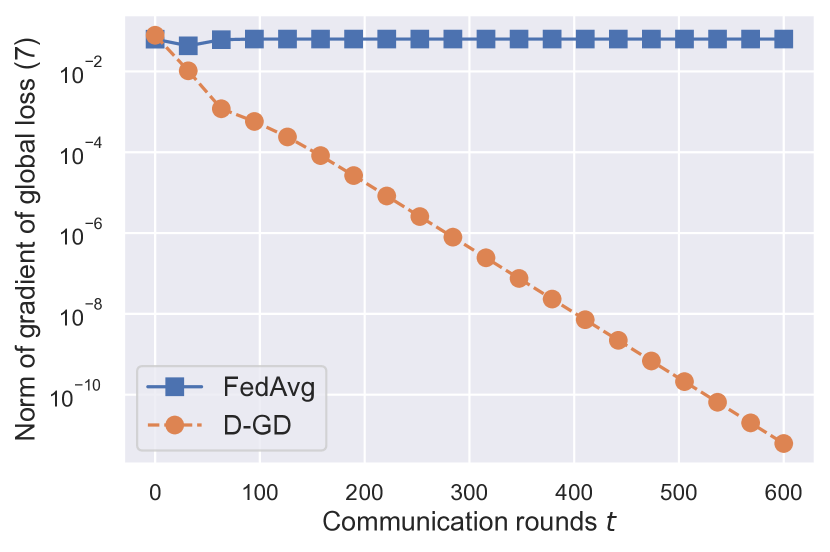
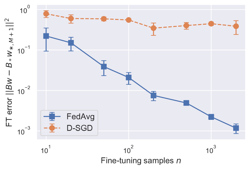
We first experiment with the regression setting from our theory. We randomly generate and by sampling each element i.i.d. from the normal distribution, where and , and then orthogonalizing . Then we run FedAvg with local updates and D-GD, both sampling clients per round. We have seen in Figure 2 that the principal angle distance between the representation learned by FedAvg and the ground-truth representation linearly converges to zero, whereas D-GD does not learn the ground-truth representation. Conversely, Figure 3 (left) tracks the gradient of the global loss (7) and shows that D-GD linearly converges to stationary point of (7), while FedAvg does not converge to one at all. Although D-GD optimizes the global loss, it does not generalize as well as FedAvg to new clients as demonstrated by Figure 3 (right). Here, we fine-tune the models learned by FedAvg and D-GD on a new client with samples generated by , , and . We fine-tune using GD for iterations with batch size , and plot the final error . Both plots are generated by averaging 10 runs.
5.2 Image classification with neural networks
Next we evaluate FedAvg’s representation learning ability on nonlinear neural networks. For fair comparison, in every experiment all methods make the same total amount of local updates during the course of training (e.g. D-SGD is trained for more rounds than FedAvg with ).
Datasets and models. We use the image classification datasets CIFAR-10 and CIFAR-100 [28], which consist of 10 and 100 classes of RGB images, respectively. We use a convolutional neural network (CNN) with three convolutional blocks followed by a three-layer multi-layer perceptron, with each convolutional block consisting of two convolutional layers and a max pooling layer.
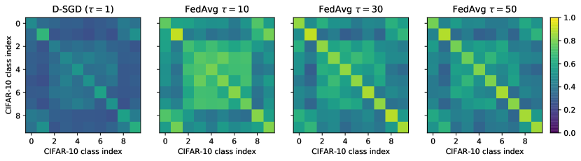
Cosine similarity of features. A desirable property of representations for downstream classification tasks is that features of examples from the same class are similar to each other, while features of examples from different classes are dissimilar [21]. In Figure 4 we examine whether the representations learned by FedAvg satisfy this property. Here we have trained FedAvg with varying and D-SGD (FedAvg with ) on CIFAR-10. Image classes are heterogeneously allocated to clients according to the Dirichlet distribution with parameter 0.6 as in [1]. Each subplot is a 10x10 matrix whose -th element gives the average cosine similarity between features of images from the -th and -th classes learned by the corresponding model. Ideally, diagonal elements are close to 1 (high similarity) and off-diagonal elements are close to 0 (low similarity). Figure 4 shows that FedAvg indeed learns features with high intra-class similarity and low inter-class similarity, with representation quality improving with more local updates between communications. Meanwhile, D-SGD does not learn such features. The leftmost subplot shows that all of the features learned by D-SGD are dissimilar, regardless of whether two images belong to the same class.
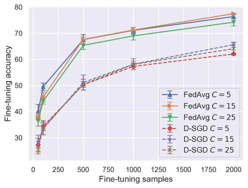
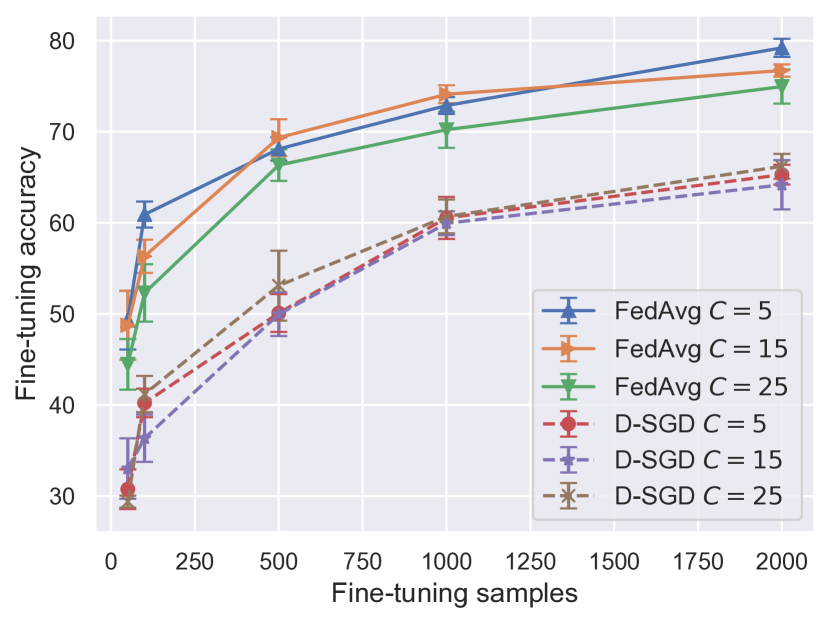
Fine-tuning performance. We evaluate the generalization ability of the representations learned by FedAvg to new classes and also new datasets. An effective representation identifies universally important features, so it should generalize to new data, with perhaps a small amount of fine-tuning needed to learn a new mapping from feature space to label space. The transfer learning performance of fine-tuned models is a popular metric for evaluating the quality of learned representations [62, 6].
We first study how models trained by FedAvg and D-SGD generalize to unseen classes from the same dataset. To do so, we train models on heterogeneous partitions of CIFAR-100 using both FedAvg with as well as D-SGD. In the left plot of Figure 5, we illustrate the case that models are trained on 80 clients each with 500 total images from classes sub-selected from 80 classes of CIFAR-100, and tested on new clients with images from the remaining 20 classes of CIFAR-100. We fine-tune the trained models on the new clients with 10 epochs of SGD, with varying numbers of samples per epoch as listed on the x-axis, before testing.
Next, we investigate how well models trained by FedAvg and D-SGD generalize to an unseen dataset. In the right plot of Figure 5, we train models with classes/client from CIFAR-100, then test on new clients with samples drawn from CIFAR-10 (a different dataset, but with presumably similar “basic” features). Specifically, for these new clients, we fine-tune for 10 epochs as previously, then test the post-fine-tuned models on the test data for each client. In both left and right plots, we observe that FedAvg significantly outperforms D-SGD, indicating that FedAvg has learned a representation that generalizes better to new classes. Additional details are provided in Appendix C.
Acknowledgements
This research of Collins, Mokhtari, and Shakkottai is supported in part by NSF Grants 2019844 and 2112471, ARO Grant W911NF2110226, ONR Grant N00014-19-1-2566, the Machine Learning Lab (MLL) at UT Austin, and the Wireless Networking and Communications Group (WNCG) Industrial Affiliates Program. The research of Hassani is supported by NSF Grants 1837253, 1943064, AFOSR Grant FA9550-20-1-0111, DCIST-CRA, and the AI Institute for Learning-Enabled Optimization at Scale (TILOS).
References
- [1] Durmus Alp Emre Acar, Yue Zhao, Ramon Matas, Matthew Mattina, Paul Whatmough, and Venkatesh Saligrama. Federated learning based on dynamic regularization. In International Conference on Learning Representations, 2021.
- [2] Manoj Ghuhan Arivazhagan, Vinay Aggarwal, Aaditya Kumar Singh, and Sunav Choudhary. Federated learning with personalization layers. arXiv preprint arXiv:1912.00818, 2019.
- [3] Zachary Charles and Jakub Konečnỳ. On the outsized importance of learning rates in local update methods. arXiv preprint arXiv:2007.00878, 2020.
- [4] Zachary Charles and Jakub Konečnỳ. Convergence and accuracy trade-offs in federated learning and meta-learning. In International Conference on Artificial Intelligence and Statistics, pages 2575–2583. PMLR, 2021.
- [5] Shuxiao Chen, Qinqing Zheng, Qi Long, and Weijie J Su. A theorem of the alternative for personalized federated learning. arXiv preprint arXiv:2103.01901, 2021.
- [6] Ting Chen, Simon Kornblith, Mohammad Norouzi, and Geoffrey Hinton. A simple framework for contrastive learning of visual representations. In International conference on machine learning, pages 1597–1607. PMLR, 2020.
- [7] Wenlin Chen, Samuel Horvath, and Peter Richtarik. Optimal client sampling for federated learning. arXiv preprint arXiv:2010.13723, 2020.
- [8] Gary Cheng, Karan Chadha, and John Duchi. Fine-tuning is fine in federated learning. arXiv preprint arXiv:2108.07313, 2021.
- [9] Yae Jee Cho, Jianyu Wang, and Gauri Joshi. Client selection in federated learning: Convergence analysis and power-of-choice selection strategies. arXiv preprint arXiv:2010.01243, 2020.
- [10] Kurtland Chua, Qi Lei, and Jason D Lee. How fine-tuning allows for effective meta-learning. Advances in Neural Information Processing Systems, 34, 2021.
- [11] Liam Collins, Hamed Hassani, Aryan Mokhtari, and Sanjay Shakkottai. Exploiting shared representations for personalized federated learning. In International Conference on Machine Learning, pages 2089–2099. PMLR, 2021.
- [12] Liam Collins, Aryan Mokhtari, Sewoong Oh, and Sanjay Shakkottai. Maml and anil provably learn representations. arXiv preprint arXiv:2202.03483, 2022.
- [13] Simon S. Du, Wei Hu, Sham M. Kakade, Jason D. Lee, and Qi Lei. Few-shot learning via learning the representation, provably, 2020.
- [14] Alireza Fallah, Aryan Mokhtari, and Asuman Ozdaglar. Personalized federated learning: A meta-learning approach, 2020.
- [15] Chelsea Finn, Pieter Abbeel, and Sergey Levine. Model-agnostic meta-learning for fast adaptation of deep networks. In Proceedings of the 34th International Conference on Machine Learning-Volume 70, pages 1126–1135. JMLR. org, 2017.
- [16] Eduard Gorbunov, Filip Hanzely, and Peter Richtárik. Local sgd: Unified theory and new efficient methods. In International Conference on Artificial Intelligence and Statistics, pages 3556–3564. PMLR, 2021.
- [17] Robert Mansel Gower, Nicolas Loizou, Xun Qian, Alibek Sailanbayev, Egor Shulgin, and Peter Richtárik. Sgd: General analysis and improved rates. In International Conference on Machine Learning, pages 5200–5209. PMLR, 2019.
- [18] David Gross and Vincent Nesme. Note on sampling without replacing from a finite collection of matrices. arXiv preprint arXiv:1001.2738, 2010.
- [19] Farzin Haddadpour, Mohammad Mahdi Kamani, Mehrdad Mahdavi, and Viveck Cadambe. Local sgd with periodic averaging: Tighter analysis and adaptive synchronization. Advances in Neural Information Processing Systems, 32, 2019.
- [20] Farzin Haddadpour, Mohammad Mahdi Kamani, Aryan Mokhtari, and Mehrdad Mahdavi. Federated learning with compression: Unified analysis and sharp guarantees. arXiv preprint arXiv:2007.01154, 2020.
- [21] Raia Hadsell, Sumit Chopra, and Yann LeCun. Dimensionality reduction by learning an invariant mapping. In 2006 IEEE Computer Society Conference on Computer Vision and Pattern Recognition (CVPR’06), volume 2, pages 1735–1742. IEEE, 2006.
- [22] Baihe Huang, Xiaoxiao Li, Zhao Song, and Xin Yang. Fl-ntk: A neural tangent kernel-based framework for federated learning convergence analysis. arXiv preprint arXiv:2105.05001, 2021.
- [23] Sai Praneeth Karimireddy, Satyen Kale, Mehryar Mohri, Sashank Reddi, Sebastian Stich, and Ananda Theertha Suresh. Scaffold: Stochastic controlled averaging for federated learning. In International Conference on Machine Learning, pages 5132–5143. PMLR, 2020.
- [24] Ahmed Khaled, Konstantin Mishchenko, and Peter Richtárik. Tighter theory for local sgd on identical and heterogeneous data. In International Conference on Artificial Intelligence and Statistics, pages 4519–4529. PMLR, 2020.
- [25] Anastasia Koloskova, Nicolas Loizou, Sadra Boreiri, Martin Jaggi, and Sebastian Stich. A unified theory of decentralized sgd with changing topology and local updates. In International Conference on Machine Learning, pages 5381–5393. PMLR, 2020.
- [26] Weihao Kong, Raghav Somani, Sham Kakade, and Sewoong Oh. Robust meta-learning for mixed linear regression with small batches. Advances in neural information processing systems, 33:4683–4696, 2020.
- [27] Simon Kornblith, Mohammad Norouzi, Honglak Lee, and Geoffrey Hinton. Similarity of neural network representations revisited. In International Conference on Machine Learning, pages 3519–3529. PMLR, 2019.
- [28] Alex Krizhevsky, Geoffrey Hinton, et al. Learning multiple layers of features from tiny images. Citeseer, 2009.
- [29] Tian Li, Shengyuan Hu, Ahmad Beirami, and Virginia Smith. Ditto: Fair and robust federated learning through personalization. arXiv: 2012.04221, 2020.
- [30] Tian Li, Anit Kumar Sahu, Manzil Zaheer, Maziar Sanjabi, Ameet Talwalkar, and Virginia Smith. Federated optimization in heterogeneous networks. arXiv preprint arXiv:1812.06127, 2018.
- [31] Xiang Li, Kaixuan Huang, Wenhao Yang, Shusen Wang, and Zhihua Zhang. On the convergence of fedavg on non-iid data. In International Conference on Learning Representations, 2019.
- [32] Paul Pu Liang, Terrance Liu, Liu Ziyin, Ruslan Salakhutdinov, and Louis-Philippe Morency. Think locally, act globally: Federated learning with local and global representations. arXiv preprint arXiv:2001.01523, 2020.
- [33] Xianfeng Liang, Shuheng Shen, Jingchang Liu, Zhen Pan, Enhong Chen, and Yifei Cheng. Variance reduced local sgd with lower communication complexity. arXiv preprint arXiv:1912.12844, 2019.
- [34] Grigory Malinovskiy, Dmitry Kovalev, Elnur Gasanov, Laurent Condat, and Peter Richtarik. From local sgd to local fixed-point methods for federated learning. In International Conference on Machine Learning, pages 6692–6701. PMLR, 2020.
- [35] Andreas Maurer, Massimiliano Pontil, and Bernardino Romera-Paredes. The benefit of multitask representation learning. Journal of Machine Learning Research, 17(81):1–32, 2016.
- [36] Brendan McMahan, Eider Moore, Daniel Ramage, Seth Hampson, and Blaise Aguera y Arcas. Communication-efficient learning of deep networks from decentralized data. In Artificial Intelligence and Statistics, pages 1273–1282. PMLR, 2017.
- [37] Aritra Mitra, Rayana Jaafar, George J Pappas, and Hamed Hassani. Linear convergence in federated learning: Tackling client heterogeneity and sparse gradients. Advances in Neural Information Processing Systems, 34:14606–14619, 2021.
- [38] Tomoya Murata and Taiji Suzuki. Bias-variance reduced local sgd for less heterogeneous federated learning. In International Conference on Machine Learning, pages 7872–7881. PMLR, 2021.
- [39] Lam Nguyen, Phuong Ha Nguyen, Marten Dijk, Peter Richtárik, Katya Scheinberg, and Martin Takác. Sgd and hogwild! convergence without the bounded gradients assumption. In International Conference on Machine Learning, pages 3750–3758. PMLR, 2018.
- [40] Alex Nichol and John Schulman. Reptile: a scalable metalearning algorithm. arXiv preprint arXiv:1803.02999, 2:2, 2018.
- [41] Jaehoon Oh, Sangmook Kim, and Se-Young Yun. Fedbabu: Towards enhanced representation for federated image classification. arXiv preprint arXiv:2106.06042, 2021.
- [42] Reese Pathak and Martin J Wainwright. Fedsplit: An algorithmic framework for fast federated optimization. Advances in Neural Information Processing Systems, 33:7057–7066, 2020.
- [43] Zhaonan Qu, Kaixiang Lin, Jayant Kalagnanam, Zhaojian Li, Jiayu Zhou, and Zhengyuan Zhou. Federated learning’s blessing: Fedavg has linear speedup. arXiv preprint arXiv:2007.05690, 2020.
- [44] Sashank Reddi, Zachary Charles, Manzil Zaheer, Zachary Garrett, Keith Rush, Jakub Konečnỳ, Sanjiv Kumar, and H Brendan McMahan. Adaptive federated optimization. arXiv preprint arXiv:2003.00295, 2020.
- [45] Monica Ribero and Haris Vikalo. Communication-efficient federated learning via optimal client sampling. arXiv preprint arXiv:2007.15197, 2020.
- [46] Ohad Shamir and Nathan Srebro. Distributed stochastic optimization and learning. In 2014 52nd Annual Allerton Conference on Communication, Control, and Computing (Allerton), pages 850–857. IEEE, 2014.
- [47] Artin Spiridonoff, Alex Olshevsky, and Ioannis Paschalidis. Communication-efficient sgd: From local sgd to one-shot averaging. Advances in Neural Information Processing Systems, 34, 2021.
- [48] Sebastian U Stich. Local sgd converges fast and communicates little. In International Conference on Learning Representations, 2018.
- [49] Sebastian U Stich and Sai Praneeth Karimireddy. The error-feedback framework: Better rates for sgd with delayed gradients and compressed communication. arXiv preprint arXiv:1909.05350, 2019.
- [50] Lili Su, Jiaming Xu, and Pengkun Yang. Achieving statistical optimality of federated learning: Beyond stationary points. arXiv preprint arXiv:2106.15216, 2021.
- [51] Anand Subramanian. torch-cka. https://github.com/AntixK/PyTorch-Model-Compare, 2021.
- [52] Yue Sun, Adhyyan Narang, Ibrahim Gulluk, Samet Oymak, and Maryam Fazel. Towards sample-efficient overparameterized meta-learning. Advances in Neural Information Processing Systems, 34, 2021.
- [53] Canh T Dinh, Nguyen Tran, and Josh Nguyen. Personalized federated learning with moreau envelopes. Advances in Neural Information Processing Systems, 33:21394–21405, 2020.
- [54] Kiran K Thekumparampil, Prateek Jain, Praneeth Netrapalli, and Sewoong Oh. Statistically and computationally efficient linear meta-representation learning. Advances in Neural Information Processing Systems, 34, 2021.
- [55] Kiran Koshy Thekumparampil, Prateek Jain, Praneeth Netrapalli, and Sewoong Oh. Sample efficient linear meta-learning by alternating minimization. arXiv preprint arXiv:2105.08306, 2021.
- [56] Nilesh Tripuraneni, Chi Jin, and Michael I. Jordan. Provable meta-learning of linear representations, 2020.
- [57] Nilesh Tripuraneni, Michael Jordan, and Chi Jin. On the theory of transfer learning: The importance of task diversity. Advances in Neural Information Processing Systems, 33:7852–7862, 2020.
- [58] Jianyu Wang and Gauri Joshi. Cooperative sgd: A unified framework for the design and analysis of communication-efficient sgd algorithms. In ICML Workshop on Coding Theory for Machine Learning, 2019.
- [59] Jianyu Wang, Qinghua Liu, Hao Liang, Gauri Joshi, and H Vincent Poor. Tackling the objective inconsistency problem in heterogeneous federated optimization. arXiv preprint arXiv:2007.07481, 2020.
- [60] Jianyu Wang, Zheng Xu, Zachary Garrett, Zachary Charles, Luyang Liu, and Gauri Joshi. Local adaptivity in federated learning: Convergence and consistency. arXiv preprint arXiv:2106.02305, 2021.
- [61] Kangkang Wang, Rajiv Mathews, Chloé Kiddon, Hubert Eichner, Françoise Beaufays, and Daniel Ramage. Federated evaluation of on-device personalization. arXiv preprint arXiv:1910.10252, 2019.
- [62] William F Whitney, Min Jae Song, David Brandfonbrener, Jaan Altosaar, and Kyunghyun Cho. Evaluating representations by the complexity of learning low-loss predictors. arXiv preprint arXiv:2009.07368, 2020.
- [63] Blake Woodworth, Kumar Kshitij Patel, Sebastian Stich, Zhen Dai, Brian Bullins, Brendan Mcmahan, Ohad Shamir, and Nathan Srebro. Is local sgd better than minibatch sgd? In International Conference on Machine Learning, pages 10334–10343. PMLR, 2020.
- [64] Blake E Woodworth, Kumar Kshitij Patel, and Nati Srebro. Minibatch vs local sgd for heterogeneous distributed learning. Advances in Neural Information Processing Systems, 33:6281–6292, 2020.
- [65] Ziping Xu and Ambuj Tewari. Representation learning beyond linear prediction functions. Advances in Neural Information Processing Systems, 34, 2021.
- [66] Hao Yu, Sen Yang, and Shenghuo Zhu. Parallel restarted sgd with faster convergence and less communication: Demystifying why model averaging works for deep learning. In Proceedings of the AAAI Conference on Artificial Intelligence, volume 33, pages 5693–5700, 2019.
- [67] Tao Yu, Eugene Bagdasaryan, and Vitaly Shmatikov. Salvaging federated learning by local adaptation. arXiv preprint arXiv:2002.04758, 2020.
- [68] Fengda Zhang, Kun Kuang, Zhaoyang You, Tao Shen, Jun Xiao, Yin Zhang, Chao Wu, Yueting Zhuang, and Xiaolin Li. Federated unsupervised representation learning. arXiv preprint arXiv:2010.08982, 2020.
- [69] Fan Zhou and Guojing Cong. On the convergence properties of a -step averaging stochastic gradient descent algorithm for nonconvex optimization. arXiv preprint arXiv:1708.01012, 2017.
Appendix A Additional Related Work
In this section we provide further discussion of the related works.
Convergence of FedAvg. The convergence of FedAvg, also known as Local SGD, has been the subject of intense study in recent years, due to the algorithm’s effectiveness combined with the difficulties of analyzing it. In homogeneous data settings, local updates are easier to reconcile with solving the global objective, allowing much progress to be made in understanding convergence rates in this case [48, 19, 49, 66, 58, 19, 47, 63, 69]. In the heterogeneous case multiple works have shown that FedAvg with fixed learning rate may not solve the global objective because the local updates induce a non-vanishing bias by drifting towards local solutions, even with full gradient steps and and strongly convex objectives [31, 34, 42, 4, 59, 23, 3, 61, 60]. As a remedy, several papers have analyzed FedAvg with learning rate that decays over communication rounds, and have shown that this approach indeed reaches a stationary point of the global objective, but at sublinear rates [24, 25, 31, 43, 23] that can be strictly slower than the convergence rates of D-SGD [64, 23]. Nevertheless, in overparameterized settings with strongly convex losses, multiple works have shown that FedAvg achieves linear convergence to a global optimum [25, 43]. Here overparameterized means that the model class contains a single model that achieves zero loss for all clients. Our setting is not overparameterized in this sense, nor is it convex.
Multi-task representation learning. Multiple works have studied the multi-task linear representation learning setting [35] in recent years. [56] and [26] give statistical rates for a method-of-moments estimator for learning the representation and [52] analyze a projection and eigen-weighting based algorithm designed for the case in which ground-truth representation is unknown. Other works have studied alternating minimization procedures for learning in the context of meta-learning [54] and federated learning [11]. However, these methods require a unique head for each client, which greatly simplifies the analysis since head diversity is guaranteed prior to local updates and is not applicable to some cross-device FL settings which cannot tolerate stateful clients. Outside of the multi-task linear regression setting, [57] and [65] have demonstrated the necessity of task diversity to learning generalizable representations from a learning theoretic perspective, and [13] considered the statistical rates of representation learning by solving an ERM with unique heads per task.
Appendix B Proof of Theorem Main Results
B.1 Proof of Theorem 1
| Notation | Definition |
|---|---|
| the results of local updates of the global model at round by the -th client | |
| , respectively | |
| , i.e. product error for -th local update for task , round | |
| , such that | |
| , such that | |
| column space of , orthogonal complement to column space of , respectively |
Here the local updates are given by
and the global updates are given by
First we control the ground-truth heads sampled on each round.
Lemma 1.
Suppose . Then the event
with probability at least .
Proof.
If then holds almost surely. Otherwise, first let , and let . For any , is a set of Hermitian matrices sampled uniformly without replacement from , almost surely, and by the triangle and Cauchy-Schwarz inequalities and Definition 1. Thus, we can apply Theorem 1 in [18] to obtain
| (8) |
as long as . Choose . Note that indeed since , where is the -th standard basis vector, and . Thus we obtain
since . An analogous argument, without needing to lift the matrices to higher dimensions, yields
Union bounding, we obtain that and
with probability at least
.
Union bounding over all completes the proof.
∎
Next we state and prove the version of Theorem 1 with explicit constants. Note that the constants are not optimized.
Theorem 2 (FedAvg Representation Learning).
Consider the case that each client takes gradient steps with respect to their population loss and all losses are weighted equally in the global objective. Suppose Assumptions 1 and 2 hold, the number of clients participating each round satisfies , and the initial parameters satisfy (i) for any , (ii) and (iii) . Choose step size . Then for any , the distance of the representation learned by FedAvg with local updates satisfies after at most
communication rounds with probability at least .
Proof.
First we condition on the event , which occurs with probability at least by Lemma 1. Conditioned on this event, we will show that that the following two sets of inductive hypotheses hold for all , , and . The first set of inductive hypotheses controls local behavior. We apply the below local induction in parallel for each client at every communication round , starting from the base case .
-
1.
-
2.
-
3.
-
4.
The second set of inductions controls the global behavior, starting from as the base case:
-
1.
-
2.
-
3.
-
4.
-
5.
where . Without loss of generality let . For ease of presentation we refer to symbolically rather than by its value throughout the proof.
The above inductions are applied in the following manner. First, the global initialization at implies that the local inductive hypotheses hold after one local update (the base case). Then, by the local inductive argument, these conditions continue to hold for all subsequent local updates. This in turn implies that the global inductive hypotheses hold after the first global averaging step, i.e. and hold. Next, the global hypotheses holding at implies that the local inductions hold in their base case at (after one local update, i.e. ), which implies they continue to hold for all subsequent local updates. Again, this implies the global hypotheses hold at , which implies the base case for the local inductions at , and so on. In summary, the ordering of the inductions is:
We start by showing that the base case holds for the local inductions. The proof is identical for all and .
-
•
If : initial conditions , else .
Note that at initialization, . Likewise, at arbitrary , due to and . Thus, since , we have
as desired (recall that ).
-
•
If : initial conditions , else .
For any , we have due to either the initialization or . This implies that since is sufficiently small (noting that . Now we use and the triangle inequality to obtain:
as desired.
-
•
If : initial conditions , else .
We have
(9) By the initial conditions and by inductive hypotheses and , for any we have , , and . This implies . Therefore using (9), we obtain
(10) as desired.
-
•
If : initial conditions , else .
Now we show that the global inductions hold at global round following the local updates at round .
-
•
Initialization .
To show each of these hypotheses hold we can apply the proofs of Lemmas 6, 7 9 and 11 respectively, since they only rely on inductive hypotheses , and and appropriate scaling of and , which is guaranteed by the initialization. In particular, the proof of these inductive hypotheses is identical for all .
-
•
Initialization .
In the proof of for (Lemma 9) we leverage the fact that is close to a matrix times the average of the . Our initialization cannot guarantee that this holds for . Instead, we show that may increase from at a large rate that would cause to blow up if continued indefinitely, but since it only grows at this rate for the first round, this is ok. In particular, let such that . Then
Moreover,
by the initialization and and , thus
which implies that , as desired.
Assume that the inductive hypotheses hold up to time and local round . We first show that the local inductive hypotheses hold for local round . Then, we show that the global inductions hold at time . This is achieved by the following lemmas.
Lemma 2.
.
Proof.
Since , we have
| (13) |
where the last inequality follows by and . ∎
Lemma 3.
.
Proof.
Lemma 4.
.
Proof.
Let and . We have
We use and throughout the proof. Recall that directly implies . This bound as well as the bound on from and the Cauchy Schwarz inequality implies and , thus . Next,
where, by the Cauchy-Schwarz inequality and and
| (16) |
and
| (17) |
Thus,
| (18) |
by choice of and sufficiently small. ∎
Lemma 5.
.
Proof.
Note that
| (19) |
where the first inequality follows since (by ) and is sufficiently small, and the last inequality follows by recursively applying the first inequality for all local iterations leading up to . Thus
∎
Lemma 6.
.
Proof.
Expanding yields
| (20) |
The remainder of the proof lies in bounding the error terms, which are all terms in the RHS of (20) besides the terms in the first line. First, by and the triangle inequality, we have
Thus, by , we have
Next, we can bound the difference between the locally-updated representation and the global representation as follows, for any
| (21) |
using and to control the norms of and . From (21) it follows that
| (22) |
Also, we have by and ,
| (23) |
Thus, using these bounds with (20), we obtain
to complete the proof, where we have used that is sufficiently small in the last inequality. ∎
Lemma 7.
Proof.
By the triangle inequality and , we have
as desired. ∎
Lemma 8.
.
Proof.
First note that
| (24) | ||||
| (25) |
where is the QR factorization of . Next, we would like to show the RHS is at most . Using and , we obtain
Next we use that by choice of initialization and choice of , and similarly . Let . Then we have
Now, observe that
| (26) |
where (26) holds for all and , therefore we have
| (27) |
Thus, using (25), we obtain
as desired. ∎
Lemma 9.
Proof.
We aim to write for a positive definite matrix and a perturbation matrix . This will yield the inequality . Assuming and scale appropriately (defined later), this inequality combined with inductive hypothesis will give the desired upper bound on (this is because the upper bound on scales with , so contributes to controlling ). The proof therefore relies on showing the existence of appropriate and .
First recall and . Let , i.e. satisfies . Then
| (28) |
The key is showing that for appropriate and . Then, by (28), we will have as desired, where .
Notice that is the average across clients of the sum of their local gradients on every local update. In particular, we have
| (29) |
We will unroll the gradients for the first two local updates only, in order to obtain a negative term that will contribute to the contraction of (i.e. will be extracted from the gradients for the first two local updates). The remaining terms will belong to and must be upper bounded (i.e. can grow due to local updates beyond the second local update, but we will show that it can’t grow too much). In particular, we have
Multiplying both sides by , and using the fact that , we obtain
| (30) |
where the first term is a negative term that helps stay small, and the remaining terms are given by
| (31) |
To get from the first to the second equation we expanded the fourth term in the first equation. We need to upper bound the spectral norm of each of these terms. The matrices and are straightforward to control; we will take care of them shortly. For now we are concerned with . In order to control this matrix, we must use the fact that is close to a matrix times . This will allow us to subsume the dominant term from into the negative term in (30). In particular, note that by , we have , where . This implies that
| (32) |
Making this substitution in , we obtain,
| (33) |
The dominant term in (33) is the last term. Specifically, we have,
| (34) | ||||
| (35) |
where (34) follows by applying the Cauchy-Schwarz inequality to each of the terms in the previous inequality, and using , and our bound on (from ), and (35) follows as is sufficiently small. The last first term term can be subsumed by completing a square as follows. Combining (30), (31) and (33) yields
| (36) |
where and
we have performed the desired decomposition; it remains to show that and scale appropriately. First we lower bound .
| (37) | ||||
| (38) | ||||
| (39) |
where (37) follows by Lemma 8, (38) follows by Assumption 2 and , and (39) follows as . Now we upper bound . We have already upper bounded in (35). We next upper bound and by and . We have
using the triangle and Cauchy-Schwarz inequalities. Now we turn to . Recall that is the sum of local gradients across all clients and all local updates beyond the first local update. We show that these gradients are sufficiently small such that cannot grow beyond the desired threshold.
Recall that . To bound this sum it is critical to control the evolution of . The idea is to split into its projection onto and its projection onto Then, we can show that the magnitude of the projection onto is going to zero very fast (the head is quickly learned, meaning it fits the product as much as it can with what it has to work with, i.e. ). On the other hand, the magnitude of the projection onto is slowly going to zero, since this reducing this error requires changing the representation and the representation changes slower than the head. The saving grace is that this error is proportional to , which for all is linearly converging to zero with .
To show this, pick any and let denote the QR-factorization of . Define and . By expanding , we find
| (40) |
Therefore,
| (41) |
For the first term, we have
| (42) | ||||
| (43) | ||||
| (44) | ||||
| (45) |
where (42) follows since , (43) follows using the Cauchy-Schwarz and triangle inequalities, (44) follows using that and applying and , (45) follows by the fact that by . For the second term in (41), note that
| (46) |
As a result, we have
| (47) |
where (47) follows by , and
| (48) | ||||
| (49) |
where (48) follows since and (49) follows using the Cauchy-Schwarz inequality, , , , and . Next, recalling that is the QR-factorization of , we have, for any ,
| (50) | ||||
| (51) |
where (50) follows by Weyl’s inequality and (51) follows by . Furthermore, for any . Thus, for the third term in (41), for any ,
| (52) |
and for we have
| (53) |
Thus, using with (41), (45), (47), (49), (52), and (53), we have
where the last inequality follows by choice of . Combining all terms, we obtain
| (54) | ||||
| (55) | ||||
| (56) |
where (54) follows by choice of , (55) follows from , and the last inequality is due to .
∎
Lemma 10.
.
Proof.
We have
which implies
| (57) |
We can expand the right product of using the binomial expansion as follows:
Recall that each . Thus, after the identity, the spectral norm of the first set of summations has spectral norm at most , the second set has specral norm at most , and so on. We in fact use the first set of summations as a negative term, and bound all subsequent sets of summations as errors, exploiting the fact that their norms are geometrically decaying. In particular, we have:
| (58) |
Next, we use for all to obtain
| (59) |
Next, we have for any ,
Thus,
| (60) |
Furtheromre,
| (61) |
noting that (61) follows since we are conditioning on the event . Finally,
| (62) | |||
| (63) |
where (62) follows by Lemma 8 and Assumption 2, and (63) follows since . Combining (63), (61), (60), (59), (58), and (57), we obtain
| (64) |
using and . ∎
Lemma 11.
B.2 Proof of Proposition 1
Proposition 2 (Distributed GD lower bound).
Suppose we are in the setting described in Section 3 and . Then for any set of ground-truth heads , full-rank initialization , initial distance , step size , and number of rounds , there exists such that and , where is the result of D-GD with step size and initialization on the system with ground-truth representation and ground-truth heads .
Proof.
Recall that is the result of D-GD with step size and initialization on the system with ground-truth representation and ground-truth heads .
There are two disjoint cases: (1) for all , , or (2) there exists some such that
. If case (1) holds then the proof is complete. Otherwise, let
such that . We will show that there exists another such that , so D-GD cannot guarantee to recover the ground-truth representation, completing the proof.
Consider case (2). Without loss of generality we can write for some , , using the SVD, since . Likewise, we can write for some , . Using these decompositions, we can see that
and
| (65) |
Next, let . We first check that :
| (66) | ||||
| (67) |
as desired, where (66) follows since , and (67) follows since by the definition of the SVD. Furthermore,
| (68) |
where (68) follows from (65). Moreover, , thus . Next,
| (69) | ||||
where (69) follows since for any .
Note that for D-GD the global update for the representation is
| (70) |
and similarly, the update for the head is . Thus, the behavior of D-GD is indistinguishable in the settings with ground-truth representations since . In particular, Using this equality along with the triangle inequality yields
| (71) | ||||
| (72) | ||||
as desired, where (71) follows by the definition of case (2) and (69), and (72) follows by . ∎
Appendix C Experimental Details
C.1 Multi-task linear regression
The multi-task linear regression experiments consist of two stages: training and fine-tuning. During training, we track in Figure 2 and the Frobenius norm of the gradient of 7, i.e. , in Figure 3(left). For fine-tuning, we track the squared Euclidean distance of the post-fine-tuned model from the ground-truth in Figure 3(right) for various numbers of fine-tuning samples .
Each training trial consists of first sampling ground truth heads and a ground truth representation such that each element is i.i.d. sampled from a standard Gaussian distribution. Then, is formed by computing the QR factorization of , i.e. , where is upper triangular and has orthonormal columns. To initialize the model we set and sample such that each element is i.i.d. sampled from a standard Gaussian distribution, then compute where is the matrix with orthonormal columns resulting from the QR factorization of . Then we run FedAvg with and D-SGD on the population objective 7, with both sampling clients per round and using step size . The training plots show quantities averaged over 10 independent trials.
For each fine-tuning trial, we similarly draw a new head , and data , where . Then we run GD on the empirical loss for iterations with step size . The fine-tuning plot shows average results over 10 independent, end-to-end trials (starting with training), and the error bars give standard deviations.
C.2 Image classification
The CNN used in the image classification experiments has six convolutional layers with ReLU activations and max pooling after every other layer. On top of the six convolutional layers is a 3-layer MLP with ReLU activations.
All models are trained with a step size of after tuning in and selecting the best that yields the smallest training loss. In all cases, . We use the SGD optimizer with weight decay and momentum 0.5. We train all models such that . Thus, D-SGD trains for rounds, since in this case. Likewise, for FedAvg with , training rounds are executed. The batch size is 10 in all cases. We also experimented with larger batch sizes for D-SGD but they did not improve performance.
Each client has 500 training samples in all cases. Thus, FedAvg with is equivalent to FedAvg with one local epoch. For the experiments with classes per client for all clients, each client has the same number of images from each class. For the experiment testing fine-tuning performance on new classes from the same dataset, the first 80 classes for CIFAR100 are used for training, while classes 80-99 are reserved for new clients. For fine-tuning, 10 epochs of SGD are executed on the training data for the new client. For fine-tuning on CIFAR10, each new client has images from all 10 classes, and equal numbers of samples per class for training. For fine-tuning on CIFAR100, each new client has images from all 20 classes, with equal numbers of samples from each class for training when possible, and either 2 or 3 samples from each class otherwise (when the number of fine-tuning samples equals 50). Accuracies are top 1 accuracies evaluated on 2000 test samples per client for CIFAR10 and 400 test samples per client for the last 20 classes of CIFAR100.
To compute the layer-wise similarities in Figure 2, we use the Centered Kernel Alignment (CKA) similarity metric, which is the most common metric used to measure the similarity between neural networks [27]. CKA similarity between model layers is evaluated by feeding the same input through both networks and computing the similarity between the outputs of the layers. The similarity metric is invariant to rotations and isotropic scaling of the layer outputs [27]. We use the code from [51] to compute CKA similarity.
For Figure 4, the cosine similarity is evaluated by first feeding images from class through the trained network and storing the output of the network layer before the final linear layer to obtain the features , where each . Then, to obtain the average cosine similarity between features from classes and , we compute . We use .
All experiments were performed on two 8GB NVIDIA GeForce RTX 2070 GPUs.