An adaptive fuzzy sliding mode controller for nonlinear systems with non-symmetric dead-zone and its application to an electro-hydraulic system

Abstract

The dead-zone is one of the most common hard nonlinearities in industrial actuators and its presence may drastically compromise control systems stability and performance. In this work, an adaptive variable structure controller is proposed to deal with a class of uncertain nonlinear systems subject to a non-symmetric dead-zone input. The adopted approach is primarily based on the sliding mode control methodology but enhanced by an adaptive fuzzy algorithm to compensate the dead-zone. Using Lyapunov stability theory and Barbalat’s lemma, the convergence properties of the closed-loop system are analytically proven. In order to illustrate the controller design methodology, an application of the proposed scheme to an electro-hydraulic system is introduced. The performance of the control system is evaluated by means of numerical simulations.

I INTRODUCTION

Dead-zone is a hard nonlinearity, frequently encountered in many actuators of industrial control systems, especially those containing some very common components, such as hydraulic Knohl and Unbehauen (2000); Bessa et al. (2006); Valdiero et al. (2006) or pneumatic Guenther and Perondi (2006); Andrighetto et al. (2008); Valdiero et al. (2008) valves. Dead-zone characteristics are often unknown and it was already observed that its presence can severely reduce control system performance and lead to limit cycles in the closed-loop system.

The growing number of papers involving systems with dead-zone input confirms the importance of taking such a non-smooth nonlinearity into account during the control system design process. The most common approaches are adaptive schemes Tao and Kokotović (1994); Wang et al. (2004); Zhou et al. (2006); Ibrir et al. (2007), fuzzy systems Kim et al. (1994); Oh and Park (1998); Lewis et al. (1999); Bessa et al. (2008b), neural networks S̆elmić and Lewis (2000); Tsai and Chuang (2004); Zhang and Ge (2007) and variable structure methods Corradini and Orlando (2002); Shyu et al. (2005). Many of these works Tao and Kokotović (1994); Kim et al. (1994); Oh and Park (1998); S̆elmić and Lewis (2000); Tsai and Chuang (2004); Zhou et al. (2006) use an inverse dead-zone to compensate the negative effects of the dead-zone nonlinearity even though this approach leads to a discontinuous control law and requires instantaneous switching, which in practice can not be accomplished with mechanical actuators. An alternative scheme, without using the dead-zone inverse, was originally proposed by (Lewis et al., 1999) and also adopted by (Wang et al., 2004). In both works, the dead-zone is treated as a combination of a linear and a saturation function. This approach was further extended by (Ibrir et al., 2007) and by (Zhang and Ge, 2007), in order to accommodate non-symmetric and unknown dead-zones, respectively.

On this basis, sliding mode control can be considered as a very attractive approach because of its robustness against both structured and unstructured uncertainties as well as external disturbances. Nevertheless, the discontinuities in the control law must be smoothed out to avoid the undesirable chattering effects. The adoption of properly designed boundary layers have proven effective in completely eliminating chattering, however, leading to an inferior tracking performance.

As demonstrated by (Bessa, 2005; Bessa and Barrêto, 2010; Bessa et al., 2012, 2019), adaptive fuzzy algorithms can be properly embedded in smooth sliding mode controllers to compensate for modeling inaccuracies, in order to improve the trajectory tracking of uncertain nonlinear systems. It has also been shown that adaptive fuzzy sliding mode controllers are suitable for a variety of applications ranging from underwater robotic vehicles Bessa et al. (2007, 2008c) to the chaos control in a nonlinear pendulum Bessa et al. (2008a, 2009a).

As a matter of fact, intelligent control has proven to be a very attractive approach to cope with uncertain nonlinear systems (Bessa et al., 2005, 2017, 2018; Lima et al., 2018; Dos Santos and Bessa, 2019; Lima et al., 2020). By combining nonlinear control techniques, such as feedback linearization or sliding modes, with adaptive intelligent algorithms, for example fuzzy logic or artificial neural networks, the resulting intelligent control strategies can deal with the nonlinear characteristics as well as with modeling imprecisions and external disturbances that can arise.

In this paper, an adaptive fuzzy sliding mode controller is proposed to deal with uncertain nonlinear systems subject to a non-symmetric dead-zone input. The adopted control scheme is primarily based on the sliding mode control methodology, but an adaptive fuzzy inference system is introduced to compensate for dead-zone effects. Based on a Lyapunov-like analysis using Barbalat’s lemma, the convergence properties of the closed-loop signals are analytically proven. An application of the proposed control strategy to a third order nonlinear system (electro-hydraulic system) is introduced to illustrate the controller design process. Simulation studies are also presented in order to demonstrate the control system performance.

II PROBLEM STATEMENT

Consider a class of $n^{\mathrm{th}}$-order nonlinear system:

$$x^{(n)}=f(\mathbf{x})+b(\mathbf{x})\upsilon$$ (1)

where the scalar variable $x\in\mathbb{R}$ is the output of interest, $x^{(n)}\in\mathbb{R}$ is the $n^{\mathrm{th}}$ derivative of $x$ with respect to time $t\in[0,+\infty)$, $\mathbf{x}=[x,\dot{x},\ldots,x^{(n-1)}]\in\mathbb{R}^{n}$ is the system state vector, $f,b:\mathbb{R}^{n}\to\mathbb{R}$ are both nonlinear functions and $\upsilon\in\mathbb{R}$ represents the output of a dead-zone function $\Upsilon:\mathbb{R}\to\mathbb{R}$, as shown in Fig. 1, with $u\in\mathbb{R}$ stating for the controller output variable.

Figure 1: Dead-zone nonlinearity.

The adopted dead-zone model is mainly based on that proposed in Ibrir et al. (2007), which can be mathematically described by

$$\upsilon=\Upsilon(u)=\left\{\begin{array}[]{ll}m_{l}(u-\delta_{l})&\mbox{if}\quad u\leq\delta_{l}\\ 0&\mbox{if}\quad\delta_{l}<u<\delta_{r}\\ m_{r}(u-\delta_{r})&\mbox{if}\quad u\geq\delta_{r}\end{array}\right.$$ (2)

In respect of the dead-zone model presented in Eq. (2), the following assumptions can be made:

Assumption 1

The dead-zone output $\upsilon$ is not available to be measured.

Assumption 2

The dead-band parameters $\delta_{l}$ and $\delta_{r}$ are unknown but bounded and with known signs, i.e., $\delta_{l\,\mathrm{min}}\leq\delta_{l}\leq\delta_{l\,\mathrm{max}}<0$ and $0<\delta_{r\,\mathrm{min}}\leq\delta_{r}\leq\delta_{r\,\mathrm{max}}$.

Assumption 3

The slopes in both sides of the dead-zone are unknown but positive and bounded, i.e., $0<m_{l\,\mathrm{min}}\leq m_{l}\leq m_{l\,\mathrm{max}}$ and $0<m_{r\,\mathrm{min}}\leq m_{r}\leq m_{r\,\mathrm{max}}$

For control purposes, Eq. (2) can be rewritten in a more appropriate form:

$$\upsilon=\Upsilon(u)=m(u)[u-d(u)]$$ (3)

where

$$m(u)=\left\{\begin{array}[]{ll}m_{l}&\mbox{if}\quad u\leq 0\\ m_{r}&\mbox{if}\quad u>0\end{array}\right.$$ (4)

and

$$d(u)=\left\{\begin{array}[]{ll}\delta_{l}&\mbox{if}\quad u\leq\delta_{l}\\ u&\mbox{if}\quad\delta_{l}<u<\delta_{r}\\ \delta_{r}&\mbox{if}\quad u\geq\delta_{r}\end{array}\right.$$ (5)

Remark 1

From Assumption 2 and Eq. (5), it can be easily verified that $d(u)$ is bounded: $|d(u)|\leq\delta$, where $\delta=\mathrm{max}\{-\delta_{l\,\mathrm{min}},\delta_{r\,\mathrm{max}}\}$.

In respect of the dynamic system presented in Eq. (1), the following assumptions can also be made:

Assumption 4

The function $f$ is unknown but bounded by a known function of $\mathbf{x}$, i.e., $|\hat{f}(\mathbf{x})-f(\mathbf{x})|\leq F(\mathbf{x})$ where $\hat{f}$ is an estimate of $f$.

Assumption 5

The input gain $b(\mathbf{x})$ is unknown but positive and bounded, i.e., $0<b_{\mathrm{min}}\leq b(\mathbf{x})\leq b_{\mathrm{max}}$.

III CONTROLLER DESIGN

The proposed control problem is to ensure that, even in the presence of parametric uncertainties, unmodeled dynamics and a non-symmetric dead-zone input, the state vector $\mathbf{x}$ will follow a desired trajectory $\mathbf{x}_{d}=[x_{d},\dot{x}_{d},\ldots,x^{(n-1)}_{d}]$ in the state space.

Regarding the development of the control law, the following assumptions should also be made:

Assumption 6

The state vector $\mathbf{x}$ is available.

Assumption 7

The desired trajectory $\mathbf{x}_{d}$ is once differentiable in time. Furthermore, every element of vector $\mathbf{x}_{d}$, as well as $x^{(n)}_{d}$, is available and with known bounds.

Now, let $\tilde{x}=x-x_{d}$ be defined as the tracking error in the variable $x$, and

$$\mathbf{\tilde{x}}=\mathbf{x}-\mathbf{x}_{d}=[\tilde{x},\dot{\tilde{x}},\ldots,\tilde{x}^{(n-1)}]$$

as the tracking error vector.

Consider a sliding surface $S$ defined in the state space by the equation $s(\mathbf{\tilde{x}})=0$, with the function $s:\mathbb{R}^{n}\rightarrow\mathbb{R}$ satisfying

$$s(\mathbf{\tilde{x}})=\left(\frac{d}{dt}+\lambda\right)^{n-1}\tilde{x}$$

or conveniently rewritten as

$$s(\mathbf{\tilde{x}})=\mathbf{c^{\mathrm{T}}\tilde{x}}$$ (6)

where $\mathbf{c}=[c_{n-1}\lambda^{n-1},\ldots,c_{1}\lambda,c_{0}]$ and $c_{i}$ states for binomial coefficients, i.e.,

$$c_{i}=\binom{n-1}{i}=\frac{(n-1)!}{(n-i-1)!\>i!}\>,\quad i=0,1,\ldots,n-1$$ (7)

which makes $c_{n-1}\lambda^{n-1}+\cdots+c_{1}\lambda+c_{0}$ a Hurwitz polynomial.

From Eq. (7), it can be easily verified that $c_{0}=1$, for $\forall n\geq 1$. Thus, for notational convenience, the time derivative of $s$ will be written in the following form:

$$\dot{s}=\mathbf{c^{\mathrm{T}}\dot{\tilde{x}}}=\tilde{x}^{(n)}+\mathbf{\bar{c}^{\mathrm{T}}\tilde{x}}$$ (8)

where $\mathbf{\bar{c}}=[0,c_{n-1}\lambda^{n-1},\ldots,c_{1}\lambda]$.

Now, let the problem of controlling the uncertain nonlinear system (1) be treated in a Filippov’s way Filippov (1988), defining a control law composed by an equivalent control $\hat{u}=\widehat{bm}^{-1}(-\hat{f}+x^{(n)}_{d}-\mathbf{\bar{c}^{\mathrm{T}}\tilde{x}})$, an estimate $\hat{d}(\hat{u})$ and a discontinuous term $-K\operatorname{sgn}(s)$:

$$u=\widehat{bm}^{-1}(-\hat{f}+x^{(n)}_{d}-\mathbf{\bar{c}^{\mathrm{T}}\tilde{x}})+\hat{d}(\hat{u})-K\operatorname{sgn}(s)$$ (9)

where $\widehat{bm}=\sqrt{b_{\mathrm{max}}m_{\mathrm{max}}b_{\mathrm{min}}m_{\mathrm{min}}}$ with $m_{\mathrm{max}}=\mathrm{max}\{m_{l\,\mathrm{max}},m_{r\,\mathrm{max}}\}$ and $m_{\mathrm{min}}=\mathrm{min}\{m_{l\,\mathrm{min}},m_{r\,\mathrm{min}}\}$, $K$ is a positive gain and $\operatorname{sgn}(\cdot)$ is defined as

$$\operatorname{sgn}(s)=\left\{\begin{array}[]{rc}-1&\mbox{if}\quad s<0\\ 0&\mbox{if}\quad s=0\\ 1&\mbox{if}\quad s>0\end{array}\right.$$

Based on Assumptions 2–5 and considering that $\beta^{-1}\leq\widehat{bm}/(bm)\leq\beta$, where $\beta=\sqrt{(b_{\mathrm{max}}m_{\mathrm{max}})/(b_{\mathrm{min}}m_{\mathrm{min}})}$, the gain $K$ should be chosen according to

$$K\geq\beta\widehat{bm}^{-1}(\eta+F)+\delta+|\hat{d}(\hat{u})|+(\beta-1)|\hat{u}|$$ (10)

where $\eta$ is a strictly positive constant related to the reaching time.

Therefore, it can be easily verified that (9) is sufficient to impose the sliding condition

$$\frac{1}{2}\frac{d}{dt}s^{2}\leq-\eta|s|$$

which, in fact, ensures the finite-time convergence of the tracking error vector to the sliding surface $S$ and, consequently, its exponential stability.

In order to obtain a good approximation to $d(u)$, the estimate $\hat{d}(\hat{u})$ will be computed directly by an adaptive fuzzy algorithm.

The adopted fuzzy inference system is the zero order TSK (Takagi–Sugeno–Kang), whose rules can be stated in a linguistic manner as follows Jang et al. (1997):

If $\hat{u}$ is $\hat{U}_{r}$ then $\hat{d}=\hat{D}_{r}\>,\quad r=1,2,\ldots,N$

where $\hat{U}_{r}$ are fuzzy sets, whose membership functions could be properly chosen, and $\hat{D}_{r}$ is the output value of each one of the $N$ fuzzy rules.

Considering that each rule defines a numerical value as output $\hat{D}_{r}$, the final output $\hat{d}$ can be computed by a weighted average:

$$\hat{d}(\hat{u})=\frac{\sum_{r=1}^{N}w_{r}\cdot\>\hat{d}_{r}}{\sum_{r=1}^{N}w_{r}}$$ (11)

or, similarly,

$$\hat{d}(\hat{u})=\mathbf{\hat{D}}^{\mathrm{T}}\mathbf{\Psi}(\hat{u})$$ (12)

where, $\mathbf{\hat{D}}=[\hat{D}_{1},\hat{D}_{2},\dots,\hat{D}_{N}]$ is the vector containing the attributed values $\hat{D}_{r}$ to each rule $r$, $\mathbf{\Psi}(\hat{u})=[\psi_{1}(\hat{u}),\psi_{2}(\hat{u}),\dots,\psi_{N}(\hat{u})]$ is a vector with components $\psi_{r}(\hat{u})=w_{r}/\sum_{r=1}^{N}w_{r}$ and $w_{r}$ is the firing strength of each rule.

In order to ensure the best possible estimate $\hat{d}(\hat{u})$, the vector of adjustable parameters can be automatically updated by the following adaptation law:

$$\mathbf{\dot{\hat{D}}}=-\gamma s\mathbf{\Psi}(\hat{u})$$ (13)

where $\gamma$ is a strictly positive constant related to the adaptation rate.

It is important to emphasize that the chosen adaptation law, Eq. (13), must not only provide a good approximation to $d(u)$ but also not compromise the attractiveness of the sliding surface, as will be proven in the following theorem.

Theorem 1

Consider the uncertain nonlinear system (1) subject to the dead-zone (3) and Assumptions 1–7. Then, the controller defined by (9), (10), (12) and (13) ensures the convergence of the tracking error vector to the sliding surface $S$.

Proof: Let a positive-definite function $V$ be defined as

$$V(t)=\frac{1}{2}s^{2}+\frac{bm}{2\gamma}\mathbf{\Delta^{\mathrm{T}}\Delta}$$

where $\mathbf{\Delta}=\mathbf{\hat{D}}-\mathbf{\hat{D}}^{*}$ and $\mathbf{\hat{D}}^{*}$ is the optimal parameter vector, associated to the optimal estimate $\hat{d}^{*}(\hat{u})$. Thus, the time derivative of $V$ is

$$\dot{V}(t) =s\dot{s}+bm\gamma^{-1}\mathbf{\Delta^{\mathrm{T}}\dot{\Delta}}$$

$$=(\tilde{x}^{(n)}+\mathbf{\bar{c}^{\mathrm{T}}\tilde{x}})s+bm\gamma^{-1}\mathbf{\Delta^{\mathrm{T}}\dot{\Delta}}$$

$$=(x^{(n)}-x^{(n)}_{d}+\mathbf{\bar{c}^{\mathrm{T}}\tilde{x}})s+bm\gamma^{-1}\mathbf{\Delta^{\mathrm{T}}\dot{\Delta}}$$

$$=(f+bmu-bmd-x^{(n)}_{d}+\mathbf{\bar{c}^{\mathrm{T}}\tilde{x}})s+bm\gamma^{-1}\mathbf{\Delta^{\mathrm{T}}\dot{\Delta}}$$

$$=[f+bm\widehat{bm}^{-1}(-\hat{f}+x^{(n)}_{d}-\mathbf{\bar{c}^{\mathrm{T}}\tilde{x}})+bm\hat{d}-bmK\operatorname{sgn}(s)-bmd-(x^{(n)}_{d}-\mathbf{\bar{c}^{\mathrm{T}}\tilde{x}})]s+bm\gamma^{-1}\mathbf{\Delta^{\mathrm{T}}\dot{\Delta}}$$

Defining the minimum approximation error as $\varepsilon=\hat{d}^{*}-d$, recalling that $\hat{u}=\widehat{bm}^{-1}(-\hat{f}+x^{(n)}_{d}-\mathbf{\bar{c}^{\mathrm{T}}\tilde{x}})$, and noting that $\mathbf{\dot{\Delta}}=\mathbf{\dot{\hat{D}}}$ and $f=\hat{f}-(\hat{f}-f)$, $\dot{V}$ becomes:

$$\dot{V}(t) =-[(\hat{f}-f)-bm\varepsilon-bm(\hat{d}-\hat{d}^{*})+\widehat{bm}\hat{u}-bm\hat{u}+bmK\operatorname{sgn}(s)]s+bm\gamma^{-1}\mathbf{\Delta^{\mathrm{T}}\dot{\hat{D}}}$$

$$=-[(\hat{f}-f)-bm\varepsilon-bm(\hat{D}-\hat{D}^{*})\mathbf{\Psi}(\hat{u})+\widehat{bm}\hat{u}-bm\hat{u}+bmK\operatorname{sgn}(s)]s+bm\gamma^{-1}\mathbf{\Delta^{\mathrm{T}}\dot{\hat{D}}}$$

$$=-[(\hat{f}-f)-bm\varepsilon+\widehat{bm}\hat{u}-bm\hat{u}+bmK\operatorname{sgn}(s)]s+bm\gamma^{-1}\mathbf{\Delta}^{\mathrm{T}}[\mathbf{\dot{\hat{D}}}+\gamma s\mathbf{\Psi}(\hat{u})]$$

By applying the adaptation law (13) to $\mathbf{\dot{\hat{D}}}$:

$$\dot{V}(t)=-[(\hat{f}-f)-bm\varepsilon+\widehat{bm}^{-1}\hat{u}-bm\hat{u}+bmK\operatorname{sgn}(s)]s$$

Furthermore, considering Assumptions 2–5, defining $K$ according to (10) and verifying that $|\varepsilon|=|\hat{d}^{*}-d|\leq|\hat{d}-d|\leq|\hat{d}|+\delta$, it follows that

$$\dot{V}(t)\leq-\eta|s|$$ (14)

which implies $V(t)\leq V(0)$ and that $s$ and $\mathbf{\Delta}$ are bounded. Considering that $s(\mathbf{\tilde{x}})=\mathbf{c^{\mathrm{T}}\tilde{x}}$, it can be verified that $\mathbf{\tilde{x}}$ is also bounded. Hence, Eq. (8) and Assumption 7 implies that $\dot{s}$ is also bounded.

Integrating both sides of (14) shows that

$$\lim_{t\rightarrow\infty}\int_{0}^{t}\eta|s|\,d\tau\leq\lim_{t\rightarrow\infty}\left[V(0)-V(t)\right]\leq V(0)<\infty$$

Since the absolute value function is uniformly continuous, it follows from Barbalat’s lemma Khalil (2001) that $s\to 0$ as $t\to\infty$, which ensures the convergence of the tracking error vector to the sliding surface $S$ and completes the proof. $\square$

However, the presence of a discontinuous term in the control law leads to the well known chattering phenomenon. To overcome the undesirable chattering effects, (Slotine, 1984) proposed the adoption of a thin boundary layer, $S_{\phi}$, in the neighborhood of the switching surface:

$$S_{\phi}=\big{\{}\mathbf{\tilde{x}}\in\mathbb{R}^{n}\>\big{|}\>|s(\mathbf{\tilde{x}})|\leq\phi\big{\}}$$

where $\phi$ is a strictly positive constant that represents the boundary layer thickness.

The boundary layer is achieved by replacing the sign function by a continuous interpolation inside $S_{\phi}$. It should be noted that this smooth approximation, which will be called here $\varphi(s,\phi)$, must behave exactly like the sign function outside the boundary layer. There are several options to smooth out the ideal relay but the most common choices are the saturation function:

$$\operatorname{sat}(s/\phi)=\left\{\begin{array}[]{cc}\operatorname{sgn}(s)&\mbox{if}\quad|s/\phi|\geq 1\\ s/\phi&\mbox{if}\quad|s/\phi|<1\end{array}\right.$$

and the hyperbolic tangent function $\tanh(s/\phi)$.

In this way, to avoid chattering, a smooth version of Eq. (9) can be adopted:

$$u=\widehat{bm}^{-1}(-\hat{f}+x^{(n)}_{d}-\mathbf{\bar{c}^{\mathrm{T}}\tilde{x}})+\hat{d}(\hat{u})-K\varphi(s,\phi)$$ (15)

Nevertheless, it should be emphasized that the substitution of the discontinuous term by a smooth approximation inside the boundary layer turns the perfect tracking into a tracking with guaranteed precision problem, which actually means that a steady-state error will always remain.

Remark 2

It has been demonstrated by (Bessa, 2009) that by adopting a smooth sliding mode controller, the tracking error vector will exponentially converge to a closed region $\Phi=\{\mathbf{\tilde{x}}\in\mathbb{R}^{n}\>|\>|s(\mathbf{\tilde{x}})|\leq\phi\mbox{ and }|\tilde{x}^{(i)}|\leq\zeta_{i}\lambda^{i-n+1}\phi,i=0,1,\ldots,n-1\}$, with $\zeta_{i}$ defined as

$$\zeta_{i}=\left\{\begin{array}[]{cl}1&\mbox{for}\quad i=0\\ 1+\sum^{i-1}_{j=0}\binom{i}{j}\zeta_{j}&\mbox{for}\quad i=1,2,\ldots,n-1.\end{array}\right.$$

IV ILLUSTRATIVE EXAMPLE: ELECTRO-HYDRAULIC SYSTEM

Electro-hydraulic actuators play an essential role in several branches of industrial activity and are frequently the most suitable choice for systems that require large forces at high speeds. Their application scope ranges from robotic manipulators to aerospace systems. Another great advantage of hydraulic systems is the ability to keep up the load capacity, which in the case of electric actuators is limited due to excessive heat generation.

The electro-hydraulic system considered in this work consists of a four-way proportional valve, a hydraulic cylinder and variable load force. The variable load force is represented by a mass–spring–damper system. The schematic diagram of the system under study is presented in Fig. 2.

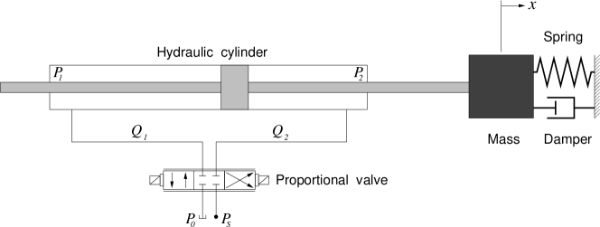
Figure 2: Schematic diagram of the electro-hydraulic servo-system.

The dynamic behavior of electro-hydraulic systems is highly nonlinear, which in fact makes the design of controllers for such systems a challenge for the conventional and well established linear control methodologies. In addition to the common nonlinearities that originate from the compressibility of the hydraulic fluid and valve flow-pressure properties, most electro-hydraulic systems are also subjected to hard nonlinearities such as dead-zone due to valve spool overlap. Considering the voltage as control input $u$ and the valve gain as dead-zone slope $m$, the valve nonlinearity can be mathematically described by Eqs. (3)–(5), with parameters $\delta_{l}$ and $\delta_{r}$ depending on the size of the overlap region.

In this way, the mathematical model that represents the electro-hydraulic system can be stated as follows Bessa et al. (2009b):

$$\dddot{x}=-\mathbf{a^{\mathrm{T}}x}+b(\mathbf{x},u)u-b(\mathbf{x},u)d(u)$$

where $\mathbf{x}=[x,\dot{x},\ddot{x}]$ is the state vector with an associated coefficient vector $\mathbf{a}=[a_{0},a_{1},a_{2}]$ defined according to

$$a_{0}=\frac{4\beta_{e}C_{tp}K_{s}}{V_{t}M_{t}}\quad;\quad a_{1}=\frac{K_{s}}{M_{t}}+\frac{4\beta_{e}A_{p}^{2}}{V_{t}M_{t}}+\frac{4\beta_{e}C_{tp}B_{t}}{V_{t}M_{t}}\quad;\quad a_{2}=\frac{B_{t}}{M_{t}}+\frac{4\beta_{e}C_{tp}}{V_{t}}$$

and

$$b(\mathbf{x},u)=\frac{4\beta_{e}A_{p}}{V_{t}M_{t}}C_{d}wm\sqrt{\frac{1}{\rho}\big{[}P_{s}-\operatorname{sgn}(u)\big{(}M_{t}\ddot{x}+B_{t}\dot{x}+K_{s}{x}\big{)}/A_{p}\big{]}}$$

Here, $x$ is the piston displacement, $M_{t}$ the total mass of piston and load referred to piston, $B_{t}$ the viscous damping coefficient of piston and load, $K_{s}$ the load spring constant, $A_{p}$ the ram area of the two chambers (symmetrical cylinder), $C_{tp}$ the total leakage coefficient of piston, $V_{t}$ the total volume under compression in both chambers, $\beta_{e}$ the effective bulk modulus, $C_{d}$ the discharge coefficient, $w$ the valve orifice area gradient, $\rho$ the hydraulic fluid density and $P_{s}$ the supply pressure

On this basis, according to the previously described control scheme and considering $s=\ddot{\tilde{x}}+2\lambda\dot{\tilde{x}}+\lambda^{2}\tilde{x}$, the smooth control law can be defined as follows

$$u=\hat{b}^{-1}(\mathbf{\hat{a}^{\mathrm{T}}x}+\dddot{x}_{d}-2\lambda\ddot{\tilde{x}}-\lambda^{2}\dot{\tilde{x}})+\hat{d}(\hat{u})-K\operatorname{sat}(s/\phi)$$

The simulation studies were performed with a numerical implementation in C, with sampling rates of 400 Hz for control system and 800 Hz for dynamic model. The adopted parameters for the electro-hydraulic system were $P_{s}=7$ MPa, $\rho=850$ kg/m³, $C_{d}=0.6$, $w=2.5\times 10^{-2}$ m, $A_{p}=3\times 10^{-4}$ m², $C_{tp}=2\times 10^{-12}$ m³/(s Pa), $\beta_{e}=700$ MPa, $V_{t}=6\times 10^{-5}$ m³, $M_{t}=250$ kg, $B_{t}=100$ Ns/m, $K_{s}=75$ N/m, $k_{l}=1.8\times 10^{-6}$ m/V, $k_{r}=2.2\times 10^{-6}$ m/V, $\delta_{l}=-1.1$ V and $\delta_{r}=0.9$ V. For controller parameters, the following values were chosen $\lambda=8$, $\varphi=4$, $\gamma=1.2$, $\delta=1.1$, $\phi=1$, $\eta=0.1$ and $\alpha=0$.

Concerning the fuzzy inference system, triangular and trapezoidal membership functions, respectively $\mu_{\mathrm{tri}}$ and $\mu_{\mathrm{trap}}$, were adopted for $\hat{U}_{r}$, with central values defined as $C=\{-5.0\>;\>-1.0\>;\>-0.5\>;\>0.0\>;\>0.5\>;\>1.0\>;\>5.0\}\times 10^{-1}$ (see Fig. 3). It is also important to emphasize, that the vector of adjustable parameters was initialized with zero values, $\mathbf{\hat{D}=0}$, and updated at each iteration step according to the adaptation law presented in Eq. (13).

Figure 3: Adopted fuzzy membership functions.

In order to evaluate the control system performance, two numerical simulations were carried out. In the first case, it was assumed that the model parameters were perfectly known but the dead-zone width was considered unknown. Figure 4 shows the obtained results for the tracking of $x_{d}=0.5\sin(0.1t)$ m.

(a) Tracking performance.

(b) Control voltage.

(c) Tracking error.

(d) Convergence of $\hat{d}(\hat{u})$ to $d(u)$.

Figure 4: Tracking performance with unknown dead-zone and well known model parameters.

As observed in Fig. 4, the adaptive fuzzy sliding mode controller (AFSMC) is able to provide trajectory tracking with small associated error and no chattering at all. It can be also verified that the proposed control law leads to a smaller tracking error when compared with the conventional sliding mode controller (SMC), Fig. 4(c). The improved performance of AFSMC over SMC is due to its ability to compensate for dead-zone effects, Fig. 4(d). The AFSMC can be easily converted to the classical SMC by setting the adaptation rate to zero, $\varphi=0$.

In the second simulation study it was assumed that the model parameters are not exactly known. On this basis, considering a maximal uncertainty of $\pm 10\%$ over the value of $k_{v}$ and variations of $\pm 20\%$ in the supply pressure, $P_{s}=7(1+0.2\sin(x))$ MPa, the estimates $\hat{k}_{v}=2\times 10^{-6}$ m/V and $\hat{P}_{s}=7$ MPa were chosen for the computation of $\hat{b}$ in the control law. The other model and controller parameters, as well as the desired trajectory, were chosen as before. The obtained results are presented in Fig. 5.

(a) Tracking performance.

(b) Control voltage.

(c) Tracking error.

(d) Convergence of $\hat{d}(\hat{u})$ to $d(u)$.

Figure 5: Tracking performance with unknown dead-zone and uncertain model parameters.

Despite the dead-zone input and uncertainties with respect to model parameters, the AFSMC allows the electro-hydraulic actuated system to track the desired trajectory with a small tracking error, (see Fig. 5). As before, the undesirable chattering effect is not observed, Fig. 5(b). Through the comparative analysis shown in Fig. 5(c), the improved performance of the AFSMC over the uncompensated counterpart can be also clearly ascertained.

V CONCLUSIONS

The present work addresses the problem of controlling uncertain nonlinear systems subject to a non-symmetric dead-zone input. An adaptive fuzzy sliding mode controller is proposed to deal with the trajectory tracking problem. The convergence properties of the closed-loop system are analytically proven using Lyapunov stability theory and Barbalat’s lemma. To illustrate the controller design method and to evaluate its performance, the proposed scheme is applied to an electro-hydraulic system. Through numerical simulations, the improved performance over the conventional sliding mode controller is also demonstrated.

VI ACKNOWLEDGEMENTS

The author acknowledges the support of the Brazilian Research Council (CNPq).

References

- Andrighetto et al. (2008) Andrighetto, P.L., Valdiero, A.C. and Bavaresco, D., 2008. “Dead zone compensation in pneumatic servo systems”. In P.E. Miyagi, O. Horikawa and J.M. Motta, eds., ABCM Symposium Series in Mechatronics, ABCM, Rio de Janeiro, Vol. 3, pp. 501–509.
- Bessa et al. (2017) Bessa, W.M., Kreuzer, E., Lange, J., Pick, M.A. and Solowjow, E., 2017. “Design and adaptive depth control of a micro diving agent”. IEEE Robotics and Automation Letters, Vol. 2, No. 4, pp. 1871–1877. doi:10.1109/LRA.2017.2714142.
- Bessa et al. (2018) Bessa, W.M., Brinkmann, G., Duecker, D.A., Kreuzer, E. and Solowjow, E., 2018. “A biologically inspired framework for the intelligent control of mechatronic systems and its application to a micro diving agent”. Mathematical Problems in Engineering, Vol. 2018, pp. 1–16. doi:10.1155/2018/9648126.
- Bessa (2005) Bessa, W.M., 2005. Controle por Modos Deslizantes de Sistemas Dinâmicos com Zona Morta Aplicado ao Posicionamento de ROVs. Tese (D.Sc.), COPPE/UFRJ, Rio de Janeiro, Brasil.
- Bessa (2009) Bessa, W.M., 2009. “Some remarks on the boundedness and convergence properties of smooth sliding mode controllers”. International Journal of Automation and Computing, Vol. 6, No. 2, pp. 154–158.
- Bessa and Barrêto (2010) Bessa, W.M. and Barrêto, R.S.S., 2010. “Adaptive fuzzy sliding mode control of uncertain nonlinear systems”. Controle & Automação, Vol. 21, No. 2, pp. 117–126.
- Bessa et al. (2008a) Bessa, W.M., De Paula, A.S. and Savi, M.A., 2008a. “Controlling chaos in a nonlinear pendulum using an adaptive fuzzy sliding mode controller”. In CBA 2008 – Proceedings of the XVII Brazilian Conference on Automatica. Juiz de Fora, Brazil.
- Bessa et al. (2009a) Bessa, W.M., De Paula, A.S. and Savi, M.A., 2009a. “Chaos control using an adaptive fuzzy sliding mode controller with application to a nonlinear pendulum”. Chaos, Solitons & Fractals, Vol. 42, No. 2, pp. 784–791.
- Bessa et al. (2012) Bessa, W.M., De Paula, A.S. and Savi, M.A., 2012. “Sliding mode control with adaptive fuzzy dead-zone compensation for uncertain chaotic systems”. Nonlinear Dynamics, Vol. 70, No. 3, pp. 1989–2001. doi:10.1007/s11071-012-0591-z.
- Bessa et al. (2005) Bessa, W.M., Dutra, M.S. and Kreuzer, E., 2005. “Thruster dynamics compensation for the positioning of underwater robotic vehicles through a fuzzy sliding mode based approach”. In COBEM 2005 – Proceedings of the 18th International Congress of Mechanical Engineering. Ouro Preto, Brasil.
- Bessa et al. (2006) Bessa, W.M., Dutra, M.S. and Kreuzer, E., 2006. “Adaptive fuzzy control of electrohydraulic servosystems”. In CONEM 2006 – Proceedings of the IV National Congress of Mechanical Engineering. Recife, Brazil.
- Bessa et al. (2007) Bessa, W.M., Dutra, M.S. and Kreuzer, E., 2007. “Adaptive fuzzy sliding mode control of underwater robotic vehicles”. In DINAME 2007 – Proceedings of the XII International Symposium on Dynamic Problems of Mechanics. Ilhabela, Brazil.
- Bessa et al. (2008b) Bessa, W.M., Dutra, M.S. and Kreuzer, E., 2008b. “An adaptive fuzzy dead-zone compensation scheme for nonlinear systems”. In CONEM 2008 – Proceedings of the V National Congress of Mechanical Engineering. Salvador, Brazil.
- Bessa et al. (2008c) Bessa, W.M., Dutra, M.S. and Kreuzer, E., 2008c. “Depth control of remotely operated underwater vehicles using an adaptive fuzzy sliding mode controller”. Robotics and Autonomous Systems, Vol. 56, No. 8, pp. 670–677.
- Bessa et al. (2009b) Bessa, W.M., Dutra, M.S. and Kreuzer, E., 2009b. “Adaptive fuzzy sliding mode control of electro-hydraulic servo-systems”. In DINAME 2009 – Proceedings of the XIII International Symposium on Dynamic Problems of Mechanics. Angra dos Reis, Brazil.
- Bessa et al. (2019) Bessa, W.M., Otto, S., Kreuzer, E. and Seifried, R., 2019. “An adaptive fuzzy sliding mode controller for uncertain underactuated mechanical systems”. Journal of Vibration and Control, Vol. 25, No. 9, pp. 1521–1535. doi:10.1177/1077546319827393.
- Corradini and Orlando (2002) Corradini, M.L. and Orlando, G., 2002. “Robust stabilization of nonlinear uncertain plants with backlash or dead zone in the actuator”. IEEE Transactions on Control Systems Technology, Vol. 10, No. 1, pp. 158–166.
- Dos Santos and Bessa (2019) Dos Santos, J.D.B. and Bessa, W.M., 2019. “Intelligent control for accurate position tracking of electrohydraulic actuators”. Electronics Letters, Vol. 55, No. 2, pp. 78–80. doi:10.1049/el.2018.7218.
- Filippov (1988) Filippov, A.F., 1988. Differential Equations with Discontinuous Right-hand Sides. Kluwer, Dordrecht.
- Guenther and Perondi (2006) Guenther, R. and Perondi, E.A., 2006. “Cascade controlled pneumatic positioning system with lugre model based friction compensation.” Journal of the Brasilian Society of mechanical Science and Engineering, Vol. 28, No. 1, pp. 48–57.
- Ibrir et al. (2007) Ibrir, S., Xie, W.F. and Su, C.Y., 2007. “Adaptive tracking of nonlinear systems with non-symmetric dead-zone input”. Automatica, Vol. 43, pp. 522–530.
- Jang et al. (1997) Jang, J.S.R., Sun, C.T. and Mizutani, E., 1997. Neuro Fuzzy and Soft Computing: A Computational Approach to Learning and Machine Intelligence. Prentice Hall, New Jersey.
- Khalil (2001) Khalil, H.K., 2001. Nonlinear Systems. Prentice Hall, New Jersey, 3rd edition.
- Kim et al. (1994) Kim, J.H., Park, J.H., Lee, S.W. and Chong, E.K.P., 1994. “A two-layered fuzzy logic controller for systems with deadzones”. IEEE Transactions on Industrial Electronics, Vol. 41, No. 2, pp. 155–162.
- Knohl and Unbehauen (2000) Knohl, T. and Unbehauen, H., 2000. “Adaptive position control of electrohydraulic servo systems using ANN”. Mechatronics, Vol. 10, pp. 127–143.
- Lewis et al. (1999) Lewis, F.L., Tim, W.K., Wang, L.Z. and Li, Z.X., 1999. “Deadzone compensation in motion control systems using adaptive fuzzy logic control”. IEEE Transactions on Control Systems Technology, Vol. 7, No. 6, pp. 731–742.
- Lima et al. (2018) Lima, G.S., Bessa, W.M. and Trimpe, S., 2018. “Depth control of underwater robots using sliding modes and gaussian process regression”. In LARS 2018 – Proceedings of the Latin American Robotic Symposium. João Pessoa, Brazil. doi:10.1109/LARS/SBR/WRE.2018.00012.
- Lima et al. (2020) Lima, G.S., Trimpe, S. and Bessa, W.M., 2020. “Sliding mode control with gaussian process regression for underwater robots”. Journal of Intelligent & Robotic Systems, Vol. 99, No. 3, pp. 487–498. doi:10.1007/s10846-019-01128-5.
- Oh and Park (1998) Oh, S.Y. and Park, D.J., 1998. “Design of new adaptive fuzzy logic controller for nonlinear plants with unknown or time-varying dead zones”. IEEE Transactions on Fuzzy Systems, Vol. 6, No. 4, pp. 482–491.
- S̆elmić and Lewis (2000) S̆elmić, R.R. and Lewis, F.L., 2000. “Deadzone compensation in motion control systems using neural networks”. IEEE Transactions on Automatic Control, Vol. 45, No. 4, pp. 602–613.
- Shyu et al. (2005) Shyu, K.K., Liu, W.J. and Hsu, K.C., 2005. “Design of large-scale time-delayed systems with dead-zone input via variable structure control”. Automatica, Vol. 41, pp. 1239–1246.
- Slotine (1984) Slotine, J.J.E., 1984. “Sliding controller design for nonlinear systems”. International Journal of Control, Vol. 40, No. 2, pp. 421–434.
- Tao and Kokotović (1994) Tao, G. and Kokotović, P.V., 1994. “Adaptive control of plants with unknow dead-zones”. IEEE Transactions on Automatic Control, Vol. 39, No. 1, pp. 59–68.
- Tsai and Chuang (2004) Tsai, C.H. and Chuang, H.T., 2004. “Deadzone compensation based on constrained RBF neural network”. Journal of The Franklin Institute, Vol. 341, pp. 361–374.
- Valdiero et al. (2008) Valdiero, A.C., Bavaresco, D. and Andrighetto, P.L., 2008. “Experimental indentification of the dead zone in proportional directional pneumatic valves”. International Journal of Fluid Power, Vol. 9, No. 2, pp. 27–34.
- Valdiero et al. (2006) Valdiero, A.C., Guenther, R. and De Negri, V.J., 2006. “New methodology for indentification of the dead zone in proportional directional hydraulic valves”. In P.E. Miyagi, O. Horikawa and E. Villani, eds., ABCM Symposium Series in Mechatronics, ABCM, Rio de Janeiro, Vol. 2, pp. 377–384.
- Wang et al. (2004) Wang, X.S., Su, C.Y. and Hong, H., 2004. “Robust adaptive control of a class of nonlinear systems with unknow dead-zone”. Automatica, Vol. 40, pp. 407–413.
- Zhang and Ge (2007) Zhang, T.P. and Ge, S.S., 2007. “Adaptive neural control of MIMO nonlinear state time-varying delay systems with unknown dead-zones and gain signs”. Automatica, Vol. 43, pp. 1021–1033.
- Zhou et al. (2006) Zhou, J., Wen, C. and Zhang, Y., 2006. “Adaptive output control of nonlinear systems with uncertain dead-zone nonlinearity”. IEEE Transactions on Automatic Control, Vol. 51, No. 3, pp. 504–511.