On the Effect of Triadic Closure on Network Segregation

Abstract.

The tendency for individuals to form social ties with others who are similar to themselves, known as homophily, is one of the most robust sociological principles. Since this phenomenon can lead to patterns of interactions that segregate people along different demographic dimensions, it can also lead to inequalities in access to information, resources, and opportunities. As we consider potential interventions that might alleviate the effects of segregation, we face the challenge that homophily constitutes a pervasive and organic force that is difficult to push back against. Designing effective interventions can therefore benefit from identifying counterbalancing social processes that might be harnessed to work in opposition to segregation.In this work, we show that triadic closure—another common phenomenon that posits that individuals with a mutual connection are more likely to be connected to one another—can be one such process. In doing so, we challenge a long-held belief that triadic closure and homophily work in tandem. By analyzing several fundamental network models using popular integration measures, we demonstrate the desegregating potential of triadic closure. We further empirically investigate this effect on real-world dynamic networks, surfacing observations that mirror our theoretical findings. We leverage these insights to discuss simple interventions that can help reduce segregation in settings that exhibit an interplay between triadic closure and homophily. We conclude with a discussion on qualitative implications for the design of interventions in settings where individuals arrive in an online fashion, and the designer can influence the initial set of connections.

<ccs2012><concept><concept_id>10003752.10010070.10010099.10010110</concept_id><concept_desc>Theory of computation Network formation</concept_desc><concept_significance>500</concept_significance></concept><concept><concept_id>10003752.10010061.10010069</concept_id><concept_desc>Theory of computation Random network models</concept_desc><concept_significance>500</concept_significance></concept><concept><concept_id>10003752.10010070.10010099.10003292</concept_id><concept_desc>Theory of computation Social networks</concept_desc><concept_significance>500</concept_significance></concept><concept><concept_id>10002950.10003624.10003633.10003638</concept_id><concept_desc>Mathematics of computing Random graphs</concept_desc><concept_significance>500</concept_significance></concept><concept><concept_id>10010147.10010341.10010346.10010348</concept_id><concept_desc>Computing methodologies Network science</concept_desc><concept_significance>300</concept_significance></concept></ccs2012>[500]Theory of computation Network formation[500]Theory of computation Random network models[500]Theory of computation Social networks[500]Mathematics of computing Random graphs[300]Computing methodologies Network science

1. Introduction

Segregation impacts socioeconomic inequality by influencing individuals’ abilities to obtain accurate and relevant information, garner social support, and improve access to opportunity Calvo-Armengol andJackson (2004); Calvo-Armengol et al. (2009); Jacksonet al. (2012); Banerjee et al. (2013); Del Vicario et al. (2016); Zeltzer (2020); Stoicaet al. (2018); Nilizadeh et al. (2016); Hannák et al. (2017). A number of different social processes can impact segregation. Among these, homophily—the process by which individuals are more likely to form ties with whom they share similarities—is one of the most robust phenomena Lazarsfeldet al. (1954); Kossinets andWatts (2009); McPhersonet al. (2001); McPherson andSmith-Lovin (1987); Newman (2002); Shrumet al. (1988). A long line of theoretical and empirical work shows that homophily can create and amplify existing segregation. And because homophily is a potent and organic force, it is challenging to push back against without harnessing existing social processes that may already be countering its negative effects.In this work, we show that triadic closure—a process in which individuals are more likely to form ties to others with whom they share mutual connections—is one such phenomenon  Rapoport (1953); Granovetter (1977); Kossinets andWatts (2006). That is, we show that triadic closure alleviates segregation in settings where homophily is also present. Our results, which we present for a number of well-studied network formation models, challenge a long-held belief that triadic closure amplifies the effects of homophily. Such claims are frequently made, at times informally, citing concerns that homophily may lead friends-of-friends also to be similar, which would lead to further segregation under triadic closure Asikainen et al. (2020); Tóth et al. (2019); Kossinets andWatts (2009).Our work challenges this intuition: Triadic closure connects people with mutual ties, and we may therefore assume that these new links reinforce existing patterns. We find, however, that the long-range nature of triadic closure can, in fact, counteract this phenomenon. In settings where homophily is present, individuals who are similar are more likely to form ties. Consequently, if friends-of-friends are not already connected, it may be because they are dissimilar. Triadic closure can therefore expose people to dissimilar individuals, thereby decreasing segregation.Mathematically, triadic closure operates on a graph-theoretic structure called a wedge. Wedges consist of two nodes that have a neighbor in common but are themselves not linked. Triadic closure works by closing these wedges, i.e., by creating a link between these two nodes such that all three nodes are connected to one another. We analyze the effect of triadic closure on homophily by disaggregating wedges into monochromatic and bichromatic ones. The two nodes sharing a neighbor are of the same type in the case of the former but not the latter. We observe that the effect of triadic closure depends on the relative sizes of monochromatic and bichromatic wedges. We study this effect both in an absolute sense—by looking at whether network integration increases when we close a random wedge—and in a relative sense—by comparing the effect of closing a random wedge with that of closing a random edge.We provide general results for a number of well-studied models, including the stochastic block model (SBM) and a popular growing network formation model by Jackson andRogers (2007), and show that triadic closure can have positive absolute and relative effects on integration in settings where there is homophily. We use these insights to study interventions on the Jackson-Rogers model and find that small changes leveraging the effects of triadic closure can have an outsized effect on mitigating segregation in the long run. We then study the interaction of homophily, triadic closure, and segregation using a large citation network where we estimate the network formation model and find that empirically observed effects of triadic closure on integration closely match our theoretical results.Our work also generalizes a number of theoretical contributions on graph and network theory. For instance, we generalize a result about network integration from Jackson andRogers (2007) to a general network with heterogeneous nodes and with arbitrary distribution over the node types. There we provide general closed-form solutions for the time dynamic of network integration. Putting the relationship between triadic closure and homophily on a theoretical footing to ask these questions from a mathematical lens is a recent undertaking; in one formalization, Asikainen et al. (2020) propose a model that combines triadic closure and random link rewiring with an underlying level of choice homophily, in which nodes have a base preference for linking based on similarity. They show that the combination of these forces amplifies existing patterns of homophily. We examine these findings to show that this model introduces homophily even into the triadic closure process itself. We study a general variant of the Asikainen et al. (2020) model and show that triadic closure mitigates segregation when all wedges are equally likely to close under triadic closure.The remainder of the paper is organized as follows:In Section 2, we present an analysis of triadic closure in the stochastic block model, deriving mathematicalresults on its absolute and relative effects on integration. We then introduce and analyze a growing graph model based on the Jackson-Rogers model, considering the effect of triadic closure on its equilibrium state integration in Section 3. We then tackle the design of interventions that act on the initial phase of making friendships to optimize network integration. In Section 4, we study a variant of the Asikainen et al. (2020) model and show that in settings where triadic closure is not a priori biased in favor of monochromatic wedges, we obtain results consistent with our above findings. Finally, we study our results empirically using a large citation network and show that we can effectively model the network formation process in Section 5. We also find that the effects of triadic closure on integration closely match our theoretical findings. We close with a discussion of related works as well as the interplay of homophily, triadic closure, integration, and implications for network interventions on- and off-line settings in Sections 6 and 7.

2. Triadic Closure in The Stochastic Block Model

We begin by introducing notations and terminology which we will use throughout this paper: Let $G$ be a heterogeneous network, i.e., a network where nodes have a type, which may, for instance, correspond to membership in a demographic group. We assume that there are $K$ types. We denote the type of node $i$ with $type(i)$. We say an edge $(i,j)$ is monochromatic if $type(i)=type(j)$ and bichromatic otherwise.Following convention, we measure network integration using the fraction of bichromatic edges. We denote the level of network integration at time $t$ by $f(t)$. Smaller values correspond to more-segregated networks.A triplet of nodes $(i,h,j)$ is called a wedge if there exist edges $(i,h)$ and $(h,j)$ but not $(i,j)$. A wedge is said to be monochromatic if $i$ and $j$ are of the same type and bichromatic if they are not. As is common in many studies of triadic closure, we assume that all wedges are equally likely to close under triadic closure. This is due to the fact that triadic closure is designed to capture the phenomena where the presence of node $h$ in the wedge $(i,h,j)$ impacts whether or not edge $(i,j)$ is eventually formed, regardless of the node types.In this section, we study Stochastic Block Models (SBM). Under SBM, we assign independent probabilities to the existence of different edges, where these probabilities depend on the types of the corresponding nodes. Given nodes $i$ and $j$, edge $(i,j)$ is formed with probability $p\in[0,1]$ if $i$ and $j$ are of the same type and with probability $q\in[0,1]$ if they are not. We say there is homophily if and only if $p>q$.We study the effect of triadic closure in this model post network formation. That is, after the network is formed, we select and close a random wedge and measure the change in network integration. As is common in other studies on the influence of triadic closure, we first study the absolute effect by comparing the state of network integration before and after the intervention. Our work also explores the relative effect of triadic closure by considering an alternative mechanism as the baseline against which we compare the effect. We propose closing a random edge as this alternative mechanism and define relative effect as the difference in integration resulting from closing a random wedge versus a random edge.

2.1. Absolute and Relative Effects of Triadic Closure

We show that triadic closure improves network integration if and only if there is homophily. main-pratenddefaultcategory.tex

Theorem 2.1.

For any SBM network $G$ with $K\geq 2$ types each consisting of $n_{k}$ nodes, where $k\in[K]$, for sufficiently large values of $n_{k}$, triadic closure has positive absolute effect on network integration if and only if $p>q$.

See proof in .main-pratenddefaultcategory.texThe proof first shows that closing a random wedge increases network integration if and only if the ratio of bichromatic wedges to monochromatic wedges is larger than the ratio of bichromatic edges to monochromatic edges. We then approximate the number of wedges and edges with their expected values and show that homophily is a necessary and sufficient condition to achieve the stated result. We note that this result holds for any number of types as well as for cases where the types may be imbalanced in size, i.e., there may be a majority-minority partition.Triadic closure may be improving integration simply because we are adding an edge and not because of the type of edge that was added. To untangle the effect of edge addition with that of triadic closure, we turn our attention to the relative effect.

Theorem 2.2.

Consider the baseline of adding a random edge to an SBM network $G$ with $K\geq 2$ types each consisting of $n_{k}$ nodes, where $k\in[K]$. For sufficiently large values of $n_{k}$:

1. Triadic closure has a negative relative effect on network integration if $p>q$,

2. Triadic closure has positive or neutral relative effect on network integration if and only if $q\geq p\geq q\,l^{*}$, where

   $$l^{*}=\frac{2(\sum_{k}n_{k})(\sum_{k}n_{k}^{2})^{2}-(\sum_{k}n_{k})^{2}(\sum_{k}n_{k}^{3})-(\sum_{k}n_{k}^{2})(\sum_{k}n_{k}^{3})}{(\sum_{k}n_{k}^{3})\big{(}(\sum_{k}n_{k})^{2}-(\sum_{k}n_{k}^{2})\big{)}}\leq 1.$$

See proof in .main-pratenddefaultcategory.texFor the case of balanced groups (i.e., when the $n_{k}$ are all equal), Theorem 2.2 simplifies to:

Corollary 2.3.

For any SBM network $G$ with $K\geq 2$ balanced types each consisting of $n/K$ nodes, for sufficiently large values of $n/K$, triadic closure has a neutral relative effect if $p=q$ and negative relative effect if $p>q$.

Proof.

This follows from Theorem 2.2 if we set $n_{k}=\frac{n}{K}$, which results in $l^{*}=1$.∎

These above results show that we can obtain diverging conclusions when we consider absolute versus relative effects of triadic closure. In doing so, they highlight the need for further precision in examining the interaction between triadic closure, homophily, and related social phenomena. Namely, to isolate the effect of social phenomena such as triadic closure, we may need to set appropriate baselines against which we are comparing their effect.We considered adding a random edge as a natural baseline in our setting but also note that a random edge is likely to be bichromatic. Another baseline we may consider is adding a homophilous random edge, i.e., rather than adding a random edge, we favor monochromatic edges using a factor $\gamma\geq 1$. Let $o_{m}$ and $o_{b}$ be the expected number of monochromatic and bichromatic missing edges. The expected increase in the number of bichromatic edges after adding a $\gamma$-homophilous edge is approximately $\frac{o_{b}}{o_{b}+\gamma o_{m}}$. Theorem 2.4 shows that, compared to adding a homophilous edge, triadic closure has a positive relative effect if the network is sufficiently heterophilous.

Theorem 2.4.

Consider the baseline of adding a $\gamma$-homophilous random edge to an SBM network $G$ with $K\geq 2$ types consisting of $n_{k}$ nodes, where $k\in[K]$. For sufficiently large values of $n_{k}$, triadic closure has positive or neutral relative effect on network integration if and only if $q\,u(\gamma)\geq p\geq q\,l(\gamma)$, where $u(\gamma)\geq 1$ and $l(\gamma)\leq 1$.

See proof in .main-pratenddefaultcategory.texNote that for given $p$ and $q$, solving for $u(\gamma^{*})=\frac{p}{q}$ if $p\geq q$ or $l(\gamma^{*})=\frac{p}{q}$ if $p<q$, provides an equivalence notion for the effect of triadic closure. In this case, the effect of closing a random wedge on network integration is the same as adding a $\gamma^{*}$-homophilous edge to the network.For the special case of balanced groups, Figure 2 shows $u(\gamma)$ and $l(\gamma)$ for different values of $K$. In this figure, the shaded area corresponds to the values of $\frac{p}{q}$ such that $u(\gamma)\geq\frac{p}{q}\geq l(\gamma)$. This is the region where triadic closure has a positive relative effect compared to adding a $\gamma$-homophilous edge. We can see that as we increase $\gamma$, triadic closure will have a more-positive effect for larger values of $p$. Further, we can see that $u(\gamma)$ increases for larger values of $K$.To see the effect of heterogeneous sizes in the groups, we consider the case where each group $k$ has $n_{k}=n_{1}\lambda^{k}$ members. So, the larger the $\lambda$, the more variance in size across groups. Figure 2 shows $u(\gamma)$ and $l(\gamma)$ for different $\lambda$ values when the number of groups is fixed. By increasing $\lambda$, we see that $u(\gamma)$ decreases, indicating that triadic closure has a less positive effect as the relative sizes between the groups increases.

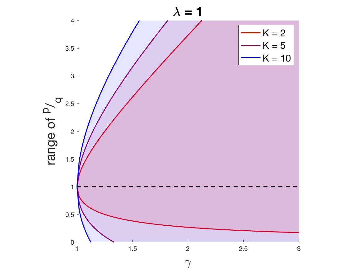
Figure 1. $u(\gamma)$ and $l(\gamma)$ for balanced groups.

For each $\gamma$, the region of $\frac{p}{q}$ such that triadic closure has a positive relative effect is plotted for different $K$s. The effect of triadic closure increases as $K$ increases.

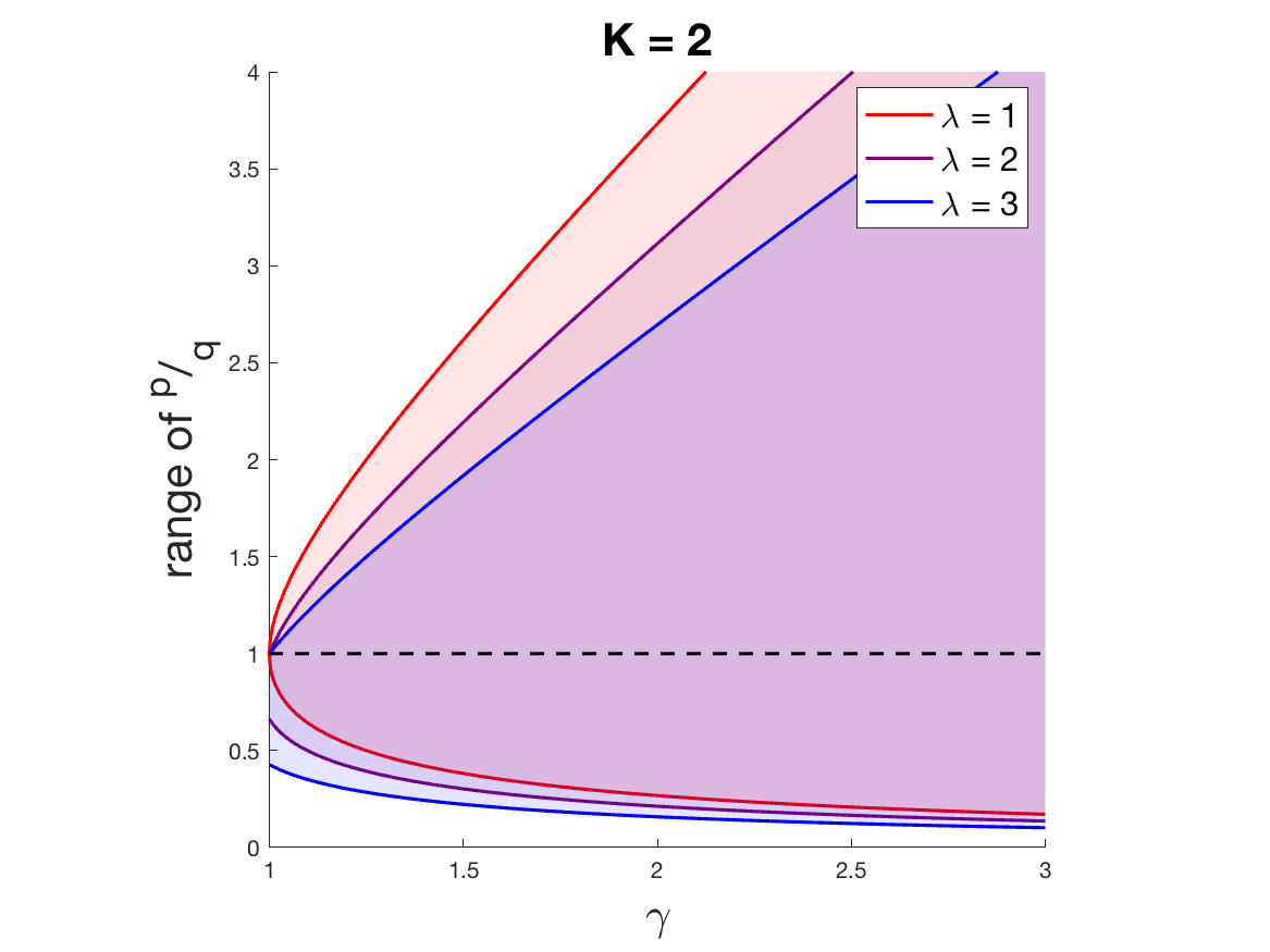
Figure 2. $u(\gamma)$ and $l(\gamma)$ for unbalanced groups ($\lambda=2$).

For each $\gamma$, the region of $\frac{p}{q}$ such that triadic closure has a positive relative effect is plotted for two groups but with different sizes. For more unbalanced groups, triadic closure is less effective.

2.2. Examining Other Measures of Network Health

Thus far, we have studied integration using a popular measure in the literature—the fraction of bichromatic edges. High rates of network integration can be observed in settings where we may otherwise consider the network to be brittle. We therefore consider another robust measure of network health using eigenvector centrality. By doing so, we show that the positive effect of triadic closure is not limited to the original measure of integration.Let ${\bm{A}}$ be the network’s adjacency matrix and ${\bm{v}}({\bm{A}})$ be the eigenvector corresponding to the largest eigenvalue of ${\bm{A}}$. The eigenvector centrality of the $i^{th}$ node is defined as ${v}_{i}({\bm{A}})$. Suppose we have a network consisting of two groups, including the setting where the groups may be imbalanced in size. Then our value of interest is the ratio of the average centrality of the minority to the average centrality of the majority group. As above, we first consider the absolute effect of triadic closure.

Theorem 2.5.

Consider an SBM network $G$ with two types consisting of $n_{1}$ and $n_{2}$ nodes, where $n_{1}>n_{2}$. Let $EV_{k}$ be the expected eigenvector centrality of a node from the $k^{th}$ group. For sufficiently large $n=n_{1}+n_{2}$, triadic closure increases $\frac{EV_{2}}{EV_{1}}$ if and only if $p>q$.

Proof.

Let $P_{ij}$ be the probability that node $i$ is connected to another node $j$ in $G$. In an $SBM$, $P_{ij}=p$ if $type(i)=type(j)$ and $P_{ij}=q$ otherwise. We also set $P^{\prime}_{ii}=0$ to avoid self loops. After closing a random wedge, we call the new network $G^{\prime}$ and the new probability that $i$ and $j$ are connected $P^{\prime}_{ij}$.Let $w_{ij}$ be the expected number of wedges in $G$, such that we have edges $(i,h)$ and $(h,j)$ exist but not $(i,j)$. Let $w$ be the expected total number of wedges. With mean field approximation:

$$P^{\prime}_{ij}=P_{ij}+(1-P_{ij})\frac{w_{ij}}{w}.$$ (1)

Here, the second term on the right hand side approximates the probability that $i$ and $j$ get connected after closing a random wedge. Note that $w=O(n^{3})$ and $w_{ij}=O(n)$, so this term is $O\left({\frac{1}{n^{2}}}\right)$. We find $w_{ij}$ based on $i$ and $j$’s types:

$$w_{ij}=\begin{cases}(n_{1}-2)p^{2}+n_{2}q^{2}&type(i)=type(j)=1\\ (n_{2}-2)p^{2}+n_{1}q^{2}&type(i)=type(j)=2\\ (n-2)pq&type(i)\neq type(j)\end{cases}.$$ (2)

By plugging $w_{ij}$ into $P^{\prime}_{ij}$, we note:

$$P^{\prime}_{ij}=\begin{cases}p^{\prime}_{1}=p+(1-p)[(n_{1}-2)p^{2}+n_{2}q^{2}]\frac{1}{w}&type(i)=type(j)=1\\ p^{\prime}_{2}=p+(1-p)[(n_{2}-2)p^{2}+n_{1}q^{2}]\frac{1}{w}&type(i)=type(j)=2\\ q^{\prime}=q+(1-q)(n-2)pq\frac{1}{w}&type(i)\neq type(j)\end{cases}.$$ (3)

Although we look for the expected eigenvector of the network, for a sufficiently large number of nodes, this quantity will be close to the eigenvector of the expected network Chung andRadcliffe (2011); Dasaratha (2017). We show the expected adjacency matrix of $G^{\prime}$ by ${\bm{A}}^{\prime}=[P^{\prime}_{ij}]$ and study eigenvectors of ${\bm{A}}^{\prime}$ instead of $G^{\prime}$.Due to the block nature of ${\bm{A}}^{\prime}$, it’s easy to see the eigenvector corresponding to the largest eigenvalue of ${\bm{A}}^{\prime}$, which we denote by ${\bm{v}}^{\prime}$, has only two distinct values. Without loss of generality, we assume ${v}^{\prime}_{i}=1$ if $type(i)=1$ and ${v}^{\prime}_{i}=a=\frac{EV_{2}}{EV_{1}}$ otherwise. That is, eigenvectors have a scale ambiguity that is usually resolved by setting the norm to one. Here, we instead fix element of the vector. Since ${\bm{A}}^{\prime}{\bm{v}}^{\prime}=\lambda{\bm{v}}^{\prime}$, we need to satisfy the following two equations:

$$(n_{1}-1)p^{\prime}_{1}+n_{2}q^{\prime}a=\lambda$$ (4)

$$n_{1}q^{\prime}+(n_{2}-1)p^{\prime}_{2}a=\lambda a$$ (5)

These give us a quadratic equation for $a$:

$$a^{2}[n_{2}q^{\prime}]+a[(n_{1}-1)p^{\prime}_{1}-(n_{2}-1)p^{\prime}_{2}]-n_{1}q^{\prime}=0.$$ (6)

Dropping $O\left({\frac{1}{n^{3}}}\right)$ from $p^{\prime}_{1}$, $p^{\prime}_{2}$, and $q^{\prime}$ and plugging into the above equation, we get:

$$a^{2}\left[{n_{2}q(1+(1-q)p\frac{n}{w})}\right]+a\left[{(n_{1}-n_{2})p\left({1+(1-p)p\frac{n}{w}}\right)}\right]-n_{1}q\left({1+(1-q)p\frac{n}{w}}\right)=0.$$ (7)

Defining $\beta=\sqrt{(n_{1}-n_{2})^{2}p^{2}+4n_{1}n_{2}q^{2}}$, the square root of the discriminant ($\Delta$) of this quadratic equation is:

$$\sqrt{\Delta}=\beta\Big{[}1+\frac{n}{w}\frac{(n_{1}-n_{2})^{2}p^{3}(1-p)+4n_{1}n_{2}pq^{2}(1-q)}{\beta^{2}}\Big{]}.$$ (8)

We can then find the solution corresponding to $a\geq 0$:

$$a=\frac{\beta-(n_{1}-n_{2})p}{2n_{2}q}+\frac{n}{w}\frac{(n_{1}-n_{2})}{n_{2}}(p-q)p^{2}\frac{\beta-(n_{1}-n_{2})p}{2q\beta}+O\left({\frac{1}{n^{3}}}\right).$$ (9)

This solution consists of two terms: The first term is exactly $\frac{EV_{2}}{EV_{1}}$ before closing a wedge. The second term is the change due to triadic closure. Since $\beta>(n_{1}-n_{2})p$, signs of $n_{1}-n_{2}$ and $p-q$ determine the effect. Given group $1$ is the majority group, the effect of triadic closure on $a$ is positive if and only if $p>q$.∎

This above theorem shows that triadic closure can improve the centrality position of a minority group in an absolute sense. As above, we also examine this in a relative sense by comparing triadic closure with adding a $\gamma$-homophilous random edge.

Theorem 2.6.

Consider the baseline of adding a $\gamma$-homophilous random edge to an SBM network $G$ with two types consisting of $n_{1}$ and $n_{2}$ nodes, where $n_{1}>n_{2}$. Let $EV_{k}$ be the expected eigenvector centrality of a node from the $k^{th}$ group. For sufficiently large $n=n_{1}+n_{2}$, triadic closure has positive relative effect on $\frac{EV_{2}}{EV_{1}}$ if and only if $\gamma>\frac{p}{q}c(p,q)$, where $c(p,q)\leq 1$. Further, $c(p,q)>\frac{q}{p}$ if $p>q$.

See proof in .main-pratenddefaultcategory.texThe proof of Theorem 2.6 follows a similar process as that of Theorem 2.5. The general idea is to approximate expected eigenvectors with eigenvectors of the expected network and then compare the change in the largest eigenvector due to adding an edge versus due to closing a wedge.We saw in Theorem 2.6 that adding a random edge, which corresponds to $\gamma=1$, is a hard-to-beat baseline. In a homophilous network, $\frac{p}{q}c(p,q)>1=\gamma$, so the relative effect is always negative. However, we can also see from this theorem that compared to a more realistic alternative ($\gamma>1$), as long as the network is not very homophilous, i.e., $\frac{p}{q}<\gamma$, triadic closure exhibits a more favorable relative performance.

3. Triadic Closure in the Jackson-Rogers Model

The Jackson-Rogers model is an evolving model originally introduced for homogeneous networks Jackson andRogers (2007) and later extended to directed heterogeneous networks Bramoullé et al. (2012). Here, we use an extended version of the model, which gives us more control over the incorporation of triadic closure.The evolution of the network is defined over discrete time steps. At each step, a new node arrives and makes new connections in two phases. In the first phase, it randomly selects $N_{S}$ and $N_{D}$ initial friends from similar and dissimilar nodes, respectively. Note that edges are directed from the new node to the older ones. In the second phase, it chooses $N_{F}$ nodes from the set of nodes accessible through an outbound edge of an initial friend. Nodes already connected to the new node are excluded from this set. This process is also biased: $\alpha$ proportion of these $N_{F}$ nodes will be selected from the friends of the similar initial friends. The rest of the connections will be equally distributed towards the friends of the dissimilar initial friends.In the explained Jackson-Rogers model, $N_{F}$ exactly accounts for triadic closure, and we can directly control it to measure the effect while the network is evolving. This corresponds to the absolute effect. However, manipulating $N_{F}$ also changes the total number of new connections per node. To distinguish the effect of triadic closure from an increased number of edges, we adopt the notion of relative effect. We say triadic closure has a positive relative effect if increasing $N_{F}$, while $N=N_{S}+N_{D}+N_{F}$ and $\frac{N_{S}}{N_{D}}$ are kept fixed, results in a higher network integration.We identify homophily in the first phase of the process by $N_{S}>N_{D}$. The definition of homophily in the second phase is not straightforward as it depends on the number of friends-of-friends of different types. Our analyses in the following sections are not sensitive to the selection of $\alpha$ as long as $0<\alpha<1$.

3.1. Absolute and Relative Effects of Triadic Closure

To study the expected behavior of an evolving network from the Jackson-Rogers model, we first prove the following theorem.

Theorem 3.1.

For an evolving Jackson-Rogers network $G$ with $K$ types and parameters $N_{S}$, $N_{D}$, $N_{F}$, and $1>\alpha>\frac{1}{K}$, the network integration converges to

$$\frac{N_{D}+(1-\alpha)N_{F}}{N_{S}+N_{D}+\frac{K}{K-1}(1-\alpha)N_{F}}$$ (10)

with the rate of $O\left({t^{-\frac{N_{S}+N_{D}}{N}}}\right)$, regardless of the distribution of node types.

See proof in .main-pratenddefaultcategory.texIn the proof of Theorem 3.1, we obtain a stronger result than the integration in equilibrium. Following Bramoullé et al. (2012), we use a mean-field approximation to find a coupled differential equation of how the composition of neighbors of a node changes over time. We find a closed-form solution to this differential equation and aggregate the behavior of individual nodes to find network integration as a function of time. Understanding the dynamic of the network in time lets us study the effect of interventions in Section 3.2.Theorem 3.1 enables us to study the effect of triadic closure on network integration in equilibrium. From this theorem, it is straightforward to see that in a network with homophily, increasing $N_{F}$, while $N_{S}$ and $N_{D}$ are unchanged, will increase network integration. We call this the absolute effect and formally state the observation in the following theorem.

Theorem 3.2.

For an evolving Jackson-Rogers network $G$ with $K$ types and parameters $N_{S}$, $N_{D}$, $N_{F}$, and $1>\alpha>\frac{1}{K}$, triadic closure has a positive absolute effect on network integration if and only if $N_{S}>\frac{N_{D}}{K-1}$.

See proof in .main-pratenddefaultcategory.texAs above, one might attribute the positive effect in Theorem 3.2 to the increased number of connections per node. Next, we show that even when the total number of edges per node and the composition of neighbors in the first phase are kept fixed, i.e., $N=N_{S}+N_{D}+N_{F}$ and $\frac{N_{S}}{N_{D}}$ are maintained, increasing $N_{F}$ will improve network integration.

Theorem 3.3.

For an evolving Jackson-Rogers network $G$ with $K$ types and parameters $N_{S}$, $N_{D}$, $N_{F}$, and $1>\alpha>\frac{1}{K}$, increasing $N_{F}$ subject to a fixed $N=N_{S}+N_{D}+N_{F}$ and $\frac{N_{S}}{N_{D}}$, results in a relative improvement in network integration if and only if $N_{S}>\frac{N_{D}}{K-1}$.

See proof in .main-pratenddefaultcategory.texIn summary, Theorems 3.2 and 3.3 show in a homophilous Jackson-Rogers evolving network, amplifying the role of triadic closure helps mitigate segregation. This effect is not due to making more connections, but rather due to the effect of triadic closure exposing nodes to dissimilar nodes.

3.2. Behavior Under a Series of Interventions

We study how interventions on a network evolving with the Jackson-Rogers model impact network integration in the short and long term. Here, we focus on interventions that act solely on the first phase. Recalling our motivating examples related to college dormitory assignments or recommendation of friendships when an individual joins an online platform, we note that an authority (i.e., university or platform, respectively) may have more leverage in this initial phase than subsequent steps which proceed through friend-of-friend searches. Such interventions that act as “nudges” in the initial phase have recently been popular in the fairness in recommender systems community; research in this space has explored the impact of bias in link formation or other selection on the long-term health of online platforms, with some work exploring the role of small nudges by the platform to mitigate inequalities or achieve other desirable social outcomes Ekstrand andWillemsen (2016); Guy (2015); Hutsonet al. (2018); Knijnenburg et al. (2016); Schnabel et al. (2018); Stoicaet al. (2018); Suet al. (2016).In our analysis of interventions, we assume that thenumber of links formed in the first phase is fixed. Thedesigner has the ability to change the proportion of mono versus bichromatic edges formed in the initial seeding phase subject to this sum constraint. This intervention imitates, for instance, dorm assignments where there is a fixed number of slots per dorm, but universities have the ability to change the composition of occupants in each dorm. We also consider the setting where the designer would like to optimize network integration subject to rate-of-change constraints on the network or on the time frame over which the intervention can occur. This is a model for scenarios where it may be costly, infeasible, or undesirable to introduce a dramatic change all at once.In the following theorem, we first find out the extent interventions can change the network integration assuming the period of intervening is very shorter than the age of the network.

Theorem 3.4.

Let $G(T)$ be an evolving Jackson-Rogers network at time $T$ with $K$ types and parameters $N_{S}$, $N_{D}$, $N_{F}$, and $1>\alpha>\frac{1}{K}$. For each $i\in[I]$, we intervene on the first phase of the evolution by setting the number of similar and dissimilar initial friends to $N_{S}^{(T+i)}$ and $N_{D}^{(T+i)}$, respectively, while the total number of initial friends is kept fixed: $N_{S}^{(T+i)}+N_{D}^{(T+i)}=N_{S}+N_{D}$. Assuming $T>>I$:

1. At time $T+I$, the expected effect of $i^{th}$ intervention on network integration is approximately

   $$-\frac{1}{N(T+I)}\Big{[}1+\frac{N_{F}}{NT}(I-i)\frac{K\alpha-1}{K-1}\Big{]}\Delta N_{S}^{(T+i)},$$ (11)

   where $\Delta N_{S}^{(T+i)}=N_{S}^{(T+i)}-N_{S}$.

2. At time $t$ when a long time is passed from $T+I$ and the network is evolved with the original parameters $N_{S}$ and $N_{D}$ after the intervention period, the expected effect of $i^{th}$ intervention on network integration is approximately

   $$-\frac{1}{N}\big{(}\frac{t}{T}\big{)}^{\frac{N_{F}}{N}\frac{K\alpha-1}{K-1}-1}\Delta N_{S}^{(T+i)}.$$ (12)

See proof in .main-pratenddefaultcategory.texEquation 11 shows two different ways that the $i^{th}$ intervention changes the network: the first term in the parenthesis corresponds to the direct impact on initial friends of the node $T+i$, and the second term explains how future nodes amplify this initial effect through triadic closure. Important observations can be made from the first part of the Theorem 3.4 which are summarized in the following corollary.

Corollary 3.5.

The immediate effect of an intervention on the network of Theorem 3.4 is

1. Independent of other interventions,

2. Negatively proportional to the change of $N_{S}$,

3. Higher if the intervention is applied earlier,

as long as the period that interventions are applied is very shorter than the age of the network ($T>>I$).

Proof.

The first argument is obvious from Equation 11; the effect of $i^{th}$ intervention only depends on $i$. The second argument comes from the fact that $K\alpha-1$ is always positive as $\alpha$ is assumed to be larger than $\frac{1}{K}$. So, the coefficient behind $\Delta N_{S}$ in Equation 11 is always negative. Finally, the effect of the $i^{th}$ intervention varies with $I-i$, so the older an intervention, the larger its effect.∎

The immediate effect of interventions (Equation 11) might look in contrast to the long-term effect (Equation 12). In fact, reducing $N_{S}$ has a positive impact on the number of bichromatic edges, which is sublinear in time. However, the number of total new edges is also increasing linearly over time, and integration is the ratio of these two numbers: $\frac{sublinear(t)}{t+T}$. As we assumed the network was old enough ($T>>1$), in the short term, the relative change of the total number of edges is small, and the effect is driven by $\approx\frac{sublinear(t)}{T}$. However, in the long term, the change in the total number of edges is not negligible, and network integration follows $\approx\frac{sublinear(t)}{t}$.Now that we can predict the expected effect an intervention has on the network, we can design optimum interventions to maximize network integration. However, there are always some constraints, e.g., the stability of the network, that limit the change a network can tolerate. We model all of these constraints as a limit on the rate of the change. The next theorem shows there is a greedy solution for optimum interventions subject to this constraint.

Theorem 3.6.

The optimum interventions of Theorem 3.4 such that

$$\max_{\{N_{S}^{(T+j)}\}_{j\in[I]}}f(T+I)$$

$$\;s.t.\;\;\forall j\in[I-1]:f(T+j+1)-f(T+j)\leq\Delta,$$

where $f(t)$ is network integration at time $t$, can be found greedily from:

$$\Delta N_{S}^{(T+j)}=\max\Big{\{}-N_{S},-NT\Delta\,\big{(}\frac{T}{T-j}\big{)}+\Big{[}1-\frac{N_{F}}{N}\frac{K\alpha-1}{K-1}\Big{]}\frac{1}{T-j}\sum_{i=1}^{j-1}\Delta N_{S}^{(T+i)}\Big{\}}.$$ (13)

If $N_{S}\geq NT\Delta(\frac{T}{T-2I})$, there is a closed-form solution for optimum interventions during $j\in[I]$:

$$\Delta N_{S}^{(T+j)}=-NT\Delta\Big{(}1+\frac{1}{T}-\frac{N_{F}}{NT}\frac{K\alpha-1}{K-1}\Big{)}^{j-1}.$$ (14)

These interventions achieve $f(T+I)-f(T)=I\,\Delta$.

Proof.

Equation 11 can be expanded to the first order of $\frac{1}{T}$ as:

$$-\frac{1}{NT}\Big{[}1+\frac{N_{F}}{NT}(I-i)\frac{K\alpha-1}{K-1}-\frac{I}{T}\Big{]}\Delta N_{S}^{(T+i)}.$$ (15)

The change of integration from time $T+j-1$ to $T+j$ due to an intervention at time $T+i$ ($i<j$) is

$$\frac{1}{NT^{2}}\Big{[}\frac{N_{F}}{N}\frac{K\alpha-1}{K-1}-1\Big{]}(-\Delta N_{S}^{(T+i)}),$$ (16)

where we simply found the difference of Equation 15 for $I=j$ and $I=j-1$. Now we can rewrite the rate of the change constraint from time $T+j-1$ to $T+j$ as:

$$\frac{1}{NT}[1-\frac{j}{T}](-\Delta N_{S}^{(T+j)})+\sum_{i=1}^{j-1}\frac{1}{NT^{2}}\Big{[}\frac{N_{F}}{N}\frac{K\alpha-1}{K-1}-1\Big{]}(-\Delta N_{S}^{(T+i)})\leq\Delta.$$ (17)

This is a linear constraint in terms of $\{\Delta N_{S}^{(T+i)}\}_{i}$. The objective function is also linear:

$$f(T+I)=\frac{1}{NT}\sum_{j=1}^{I}\Big{[}1+\frac{N_{F}}{NT}(I-j)\frac{K\alpha-1}{K-1}-\frac{I}{T}\Big{]}(-\Delta N_{S}^{(T+j)})=\sum_{j=1}^{I}c_{j}(-\Delta N_{S}^{(T+j)}).$$ (18)

Here $c_{j}$ is positive and decreasing in $j$. Let $-\Delta N_{S}^{(T+j)}=x_{j}$ ($j\in[I]$) be the optimum solution of the problem. We argue that for any $j\in[I]$, $x_{j}$ is

$$\min\Big{\{}N_{S},NT\Delta(\frac{T}{T-j})+\Big{[}1-\frac{N_{F}}{N}\frac{K\alpha-1}{K-1}\Big{]}\frac{1}{T-j}\sum_{i=1}^{j-1}x_{i}\Big{\}}.$$ (19)

Otherwise, we could increase $x_{j}$ to make the constraint of Equation 17 binding. This increase does not violate other constraints, since $\frac{N_{F}}{N}\frac{K\alpha-1}{K-1}-1<0$.Now if $N_{S}\geq NT\Delta(\frac{T}{T-2I})$, we have

$$NT\Delta(\frac{T}{T-j})+\Big{[}1-\frac{N_{F}}{N}\frac{K\alpha-1}{K-1}\Big{]}\frac{1}{T-j}\sum_{i=1}^{j-1}x_{i}\leq NT\Delta(\frac{T}{T-I})+N_{S}\frac{I}{T-I}\leq N_{S}.$$ (20)

So, $x_{j}\leq N_{S}$ is never binding and$x_{j}\approx NT\Delta+\Big{[}1-\frac{N_{F}}{N}\frac{K\alpha-1}{K-1}\Big{]}\frac{1}{T}\sum_{i=1}^{j-1}x_{i}$ for all $j\in[I]$. This is a recursive equation for $x_{j}$. Let’s define $y_{j}=\sum_{i=1}^{j}x_{j}$. The recursive definition for $y_{j}$ will be:

$$y_{j}-y_{j-1}=NT\Delta+\frac{1}{T}\Big{[}1-\frac{N_{F}}{N}\frac{K\alpha-1}{K-1}\Big{]}y_{j-1}$$ (21)

and $y_{1}=x_{1}=NT\Delta$. Taking $Z$-Transform from this recursive equation gives

$$Y(z)=\frac{NT\Delta z^{-1}}{(1-z^{-1})(1-(1+\frac{1}{T}-\frac{N_{F}}{NT}\frac{K\alpha-1}{K-1})z^{-1})}.$$ (22)

By taking $Z^{-1}$-transform of $Y(Z)$ one can see

$$y_{j}=\frac{NT\Delta}{\frac{1}{T}-\frac{N_{F}}{NT}\frac{K\alpha-1}{K-1}}\Big{[}(1+\frac{1}{T}-\frac{N_{F}}{NT}\frac{K\alpha-1}{K-1})^{j}-1\Big{]},\;\;j\geq 1$$ (23)

and Equation 14 can be obtained by $\Delta N_{S}^{(T+j)}=-x_{j}=y_{j-1}-y_{j}$.∎

4. Triadic Closure in A Fixed-Node Evolving Model

Asikainen et al. (2020) propose a model with a fixed number of nodes and edges where the network evolves through random edge addition and triadic closure. The authors argue that triadic closure increases observed homophily relative to homophilous random link formation, i.e., triadic closure has a negative relative effect.Here, we show that this result is specific to their definition of triadic closure which favors monochromatic wedges. In contrast, triadic closure is often studied in settings where wedges do not exhibit such a bias Easley andKleinberg (2010). Empirical work on real-world networks also supports this unbiased wedge closing assumption Kossinets andWatts (2006). We therefore study a variant of the Asikainen et al. (2020) model where triadic closure does not differentiate between monochromatic and bichromatic wedges.We first present the model: Consider a network with a random initial structure and where nodes belong to one of two groups. At each iteration, a focal node is selected uniformly at random. Then a candidate node is chosen by triadic closure with probability $c$ or uniformly at random with probability $1-c$. The parameter $c$ controls the relative impact of triadic closure in the evolution of the network. Let $\theta$ be the focal node type and $\theta^{\prime}$ be the candidate node type. A link is formed between focal and candidate nodes with probability $S_{\theta,\theta^{\prime}}^{\prime}$ if the candidate is selected by triadic closure and $S_{\theta,\theta^{\prime}}$ otherwise. Following Asikainen et al. (2020), we assume $S_{\theta,\theta^{\prime}}=s$ and $S_{\theta,\theta^{\prime}}^{\prime}=s^{\prime}$ if $\theta=\theta^{\prime}$, and $S_{\theta,\theta^{\prime}}=1-s$ and $S_{\theta,\theta^{\prime}}^{\prime}=1-s^{\prime}$ otherwise. To keep the number of edges constant while network is evolving, a random edge connected to the focal node is removed whenever it forms a new edge with a candidate node.In the original model of Asikainen et al. (2020), $s^{\prime}=s$ and homophily is imposed by setting $s>\frac{1}{2}$. Following the definitions above, we argue setting $s^{\prime}=s$ adds extra homophily to triadic closure. Instead, to be consistent with our definition of triadic closure, we set $s^{\prime}=\frac{1}{2}$. That is, we do not distinguish between monochromatic and bichromatic wedges. The result below shows how this change to an unbiased triadic closure setting leads to results consistent with observations in the SBM and Jackson-Rogers models.

Theorem 4.1.

For a fixed-node evolving network $G$ with two equiprobable types and parameters $s$ and $s^{\prime}=\frac{1}{2}$, triadic closure has a positive relative effect on network integration if and only if $1>s>\frac{1}{2}$, compared to a random link formation.

See proof in .main-pratenddefaultcategory.texNote that the condition $1>s>1/2$ corresponds to the setting where random link formation is homophilous. To better understand the extent to which Theorem 4.1 applies, we depict network integration theoretically estimated at equilibrium in Figure 3. We have also marked simulated results with crosses to show that the theory and empirical observations closely match one another. We note that as we increase the impact of triadic closure by increasing $c$, integration increases if $s>\frac{1}{2}$ and decreases if $s<\frac{1}{2}$. There are two extreme cases to observe: In the case of no triadic closure ($c=0$), integration falls linearly with respect to $s$. On the other extreme, when edges only form via triadic closure, i.e., $c=1$, there are two possibilities: if groups of different types are initially completely segregated, the integration will always be zero regardless of $s$. If the network is not completely segregated, the resulting integration will be $0.5$ as there was no homophily. Another interesting observation is that even when the network is maximally homophilous ($s=1$), for large enough $c$, triadic closure will not let the integration go to zero. In sum, our above result in Theorem 4.1 and corresponding simulations show that triadic closure works against segregation in homophilous networks.

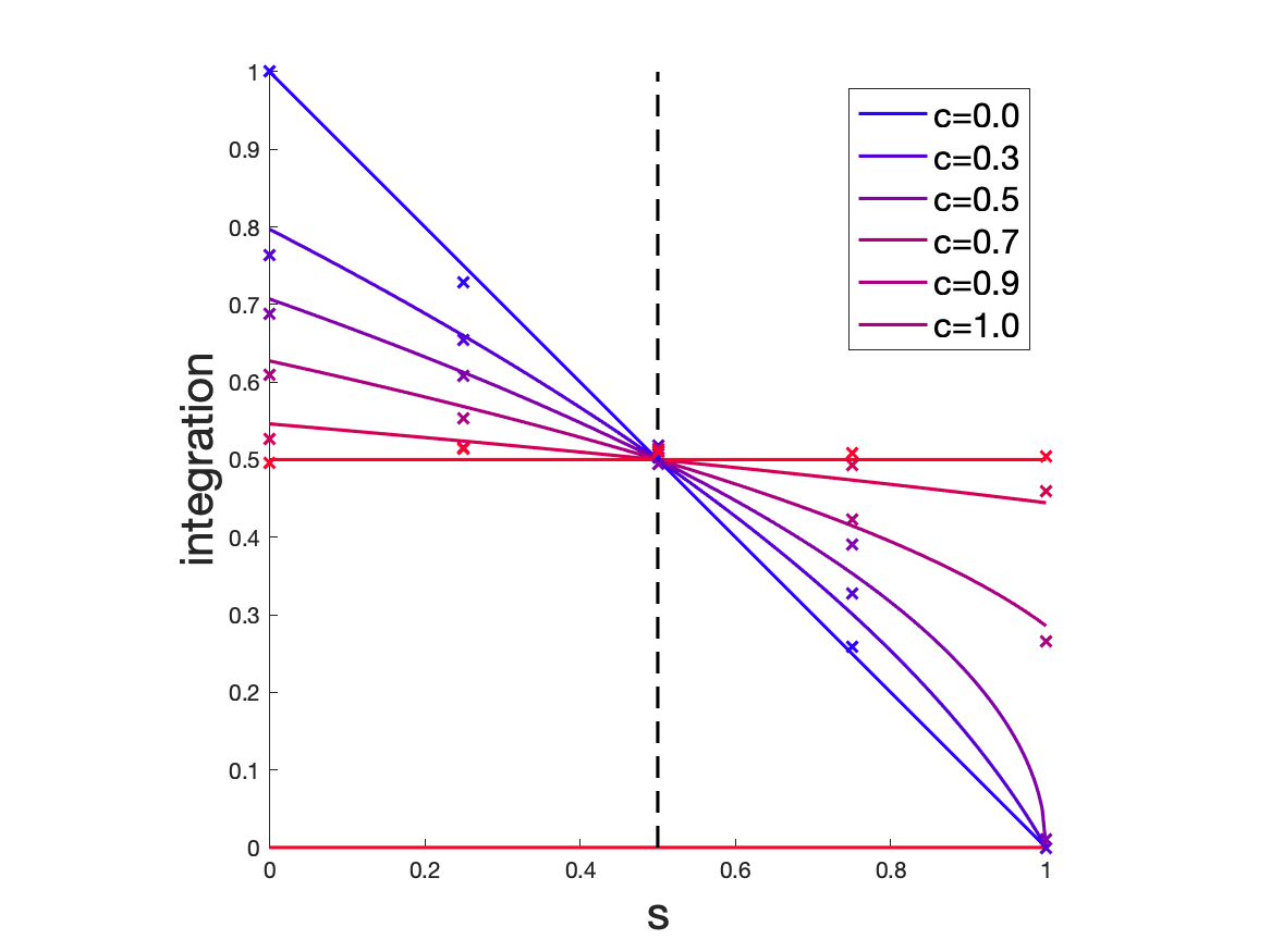
Figure 3. Network integration obtained theoretically from the fixed-node evolving model with equiprobable types and $s^{\prime}=\frac{1}{2}$. Simulation results are also marked with crosses.

Network integration is plotted vs $s$ for a fixed-node evolving model with equiprobable types and $s^{\prime}=\frac{1}{2}$. In the presence of homophily, triadic closure improves network integration.

5. Experiments

Our results so far focus on theoretical observations for the expected behavior of network properties under some approximations, for a large number of nodes, and in the limit of $t\rightarrow\infty$. In this section, we examine the validity of our results both through analysis of real data and simulations. Here we discuss the applicability of Theorem 3.1 on real data and present simulation-based evidence in Section B of the appendix.

5.1. Data: Citation Networks

The citation network we study here is known to be captured well by the Jackson-Rogers model Bramoullé et al. (2012); Jackson andRogers (2007). Several factors make the citation network consistent with this model: First, papers—which correspond to nodes on this graph—appear sequentially and do not disappear. Likewise, citations—which correspond to edges on this graph—are directed and do not disappear over time. Third, researchers often use an initial seed of articles as a foundation for their work and use the citation network to identify further related works, similar to the second phase of the Jackson-Rogers model.We use the network of citations extracted mainly from DBLP, ACM, and MAG (Microsoft Academic Graph) Tanget al. (2008) (version 12). In this dataset, each paper is labeled with weighted fields of study. We use the field of study with the highest weight as the node type. The original dataset covers papers published mainly from 1960 to 2020. However, areas of study and access to articles have experienced a tremendous change during the last decades. We therefore focus on a shorter period of 2015 to 2020 to ensure network parameters are not varying over time. This period consists of more than 1.5 million articles with more than 4.7 million intra-citations, i.e., citations within the studied network.

5.2. Estimation of Model Parameters

The citation network consists of papers from various fields. We limit our analysis to major fields of study, which we define to be fields that appear in at least $1$ percent of articles. Only $3$ percent of papers are not related to any major field.Despite the growth of interdisciplinary works, different fields of study still follow different publication traditions, resulting in different model parameters. We therefore first cluster the fields of study and then fit a separate model on each cluster, neglecting inter-cluster citations. Variation across clusters also provides further ability to test the validity of our theoretical findings.Clustering Fields of Study. In order to cluster fields, we obtain a weighted graph over major fields: Nodes correspond to fields in this graph and the weight of edge $(f_{1},f_{2})$ corresponds to how many times a paper in field $f_{1}$ has cited another paper with field $f_{2}$ or vice versa. Note that papers may have more than one field of study. We then use spectral clustering to obtain clusters of major fields. Here we selected the number of clusters to be $6$ based on the eigenvalues of the graph’s Laplacian matrix. Table 1 shows some statistics of these clusters. We chose the names of the clusters, looking at their most frequent fields.

Cluster	Num. of Fields	Num. of Papers	Num. of within-cluster citations
Mathematics	13	487,298	954,544
Artificial Intelligence	22	1,170,199	3,586,018
Knowledge Management	15	386,073	617,090
Electrical Engineering	20	474,773	1,172,721
Software Engineering	4	85,845	90,723
Control Engineering	7	254,453	355,930

Table 1. Summary statistics of the clusters of major fields reported.

Estimation of Each Cluster’s Model Parameters. Assuming the network evolves according to the Jackson-Rogers model, we want to estimate model parameters from data. These parameters include $N_{S}$, $N_{D}$, $N_{F}$, and $\alpha$. To account for the randomness of real data, we add extra randomness here: at each time step, when a new node $u$ arrives, it draws model parameters from

$$N_{S}^{(u)} \sim\exp\left({\frac{1}{n_{s}}}\right)$$

$$N_{D}^{(u)} \sim\exp\left({\frac{1}{n_{d}}}\right)$$

$$N_{F,S}^{(u)}=\alpha^{(u)}N_{F}^{(u)} \sim\exp\left({\frac{1}{n_{f,s}}}\right)$$

$$N_{F,D}^{(u)}=\left({1-\alpha^{(u)}}\right)N_{F}^{(u)} \sim\exp\left({\frac{1}{n_{f,d}}}\right).$$ (24)

Here $\exp(\lambda)$ corresponds to an exponential distribution with mean $\frac{1}{\lambda}$. We chose exponential priors only for simplicity. We believe similar results can be obtained with other positive distributions as well. Our goal is to estimate $\theta=(n_{s},n_{d},n_{f,s},n_{f,d})$.In order to estimate $\theta$, we need to distinguish edges created during phase one and phase two. Let $G(u)=({\mathcal{V}}(u),{\mathcal{E}}(u))$ be the induced subgraph of the citation graph over node (paper) $u$’s immediate descendants. Note, $G(u)$ does not include $u$. We want to know among all the edges from $u$ to ${\mathcal{V}}(u)$ which ones are formed in the first and second phases. There is no way to distinguish first and second-phase connections. Bramoullé et al. (2012) suggest that if $(v,w)\in{\mathcal{E}}(u)$, then $(u,v)$ is formed initially and $(u,w)$ is formed in the second phase due to triadic closure. However, we believe this assumption will add a bias to our estimation from model parameters. It is also not clear how to decide when there is a third node $x$ such that $(w,x)\in{\mathcal{E}}(u)$ (Figure 5). We propose an approach to estimate model parameters with minimum assumptions in the following.Let $\phi_{u}:{\mathcal{V}}(u)\rightarrow\{1,2\}$ be the phase assignment function for node $u$. $\phi_{u}(v)$ determines whether $(u,v)$ is created at the first or second phase. We call a phase assignment function feasible if for every $w\in{\mathcal{V}}(u)$ such that $\phi_{u}(w)=2$, there exists a $v\in{\mathcal{V}}(u)$ such that $(v,w)\in{\mathcal{E}}(u)$ and $\phi_{u}(v)=1$. In other words, if $(u,w)$ is assigned to be shaped in the second phase, there should be at least one mediator node that $u$ could find $w$ through it. Figure 5 shows an example of all feasible assignments of a graph with four nodes.

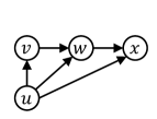
Figure 4. An example graph consists of $u$ and $G(u)$.

An example graph consists of edges $(u,v)$, $(u,w)$, $(u,x)$, $(v,w)$, and $(w,x)$.

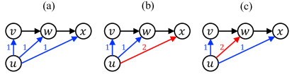
Figure 5. All feasible assignments for the edges from $u$ to $G(u)$. The numbers on the edges indicate the phase of edge formation.

Three possible assignments for the example graph are shown.

Given an assignment function and a $type(\cdot)$ function, it is straightforward to find first phase parameters for node $u$:

$$n_{s}^{(u)}(\phi_{u}) =|\{v\in{\mathcal{V}}(u)\mid\phi_{u}(v)=1,type(u)=type(v)\}|$$ (25)

$$n_{d}^{(u)}(\phi_{u}) =|\{v\in{\mathcal{V}}(u)\mid\phi_{u}(v)=1,type(u)\neq type(v)\}|.$$ (26)

However, suppose an edge like $(u,w)$ is formed in phase two, and $w$ has immediate ancestors in $G(u)$ with both similar and dissimilar types to $u$. In that case, it is not clear whether $u$ and $w$ are connected through similar initial friends of $u$ or dissimilar initial friends. Here we look at the ratio of $w$’s immediate ancestors which are similar to $u$ and use this number as an estimate for $n_{f,s}^{(u)}$.

$$n_{f,s}^{(u)}(\phi_{u}) =\sum_{w:\phi_{u}(w)=2}\frac{|\{v\in{\mathcal{V}}(u)\mid(v,w)\in{\mathcal{E}}(u),\phi_{u}(v)=1,type(v)=type(u)\}|}{|\{v\in{\mathcal{V}}(u)\mid(v,w)\in{\mathcal{E}}(u),\phi_{u}(v)=1\}|}$$ (27)

We can do the same for ancestors which are dissimilar to $u$ to estimate $n_{f,d}^{(u)}$:

$$n_{f,d}^{(u)}(\phi_{u}) =\sum_{w:\phi_{u}(w)=2}\frac{|\{v\in{\mathcal{V}}(u)\mid(v,w)\in{\mathcal{E}}(u),\phi_{u}(v)=1,type(v)\neq type(u)|\}}{|\{v\in{\mathcal{V}}(u)\mid(v,w)\in{\mathcal{E}}(u),\phi_{u}(v)=1\}|}$$ (28)

Let $\Phi_{u}$ denote the set of all feasible assignments for node $u$. We assume a uniform distribution over $\Phi_{u}$. We can now find the likelihood of observing $G(u)$ given $\theta=(n_{s},n_{d},n_{f,s},n_{f,d})$:

$$l_{u}(\theta)=\frac{1}{|\Phi_{u}|}\sum_{\phi_{u}\in\Phi_{u}}\frac{1}{n_{s}\,n_{d}\,n_{f,s}\,n_{f,d}}\exp{\Big{(}-\frac{n_{s}^{(u)}(\phi_{u})}{n_{s}}-\frac{n_{d}^{(u)}(\phi_{u})}{n_{d}}-\frac{n_{f,s}^{(u)}(\phi_{u})}{n_{f,s}}-\frac{n_{f,d}^{(u)}(\phi_{u})}{n_{f,d}}\Big{)}}$$ (29)

Finally, we maximize the likelihood of observing the whole cluster as it is to find the optimum parameters:

$$\theta^{*}=\operatorname*{arg\,max}_{\theta}\sum_{u}\log{(l_{u}(\theta))}.$$ (30)

We use the BFGS algorithm for the optimization; note, however, that this is a non-convex problem, and there is no guarantee that we can find the global maximum.

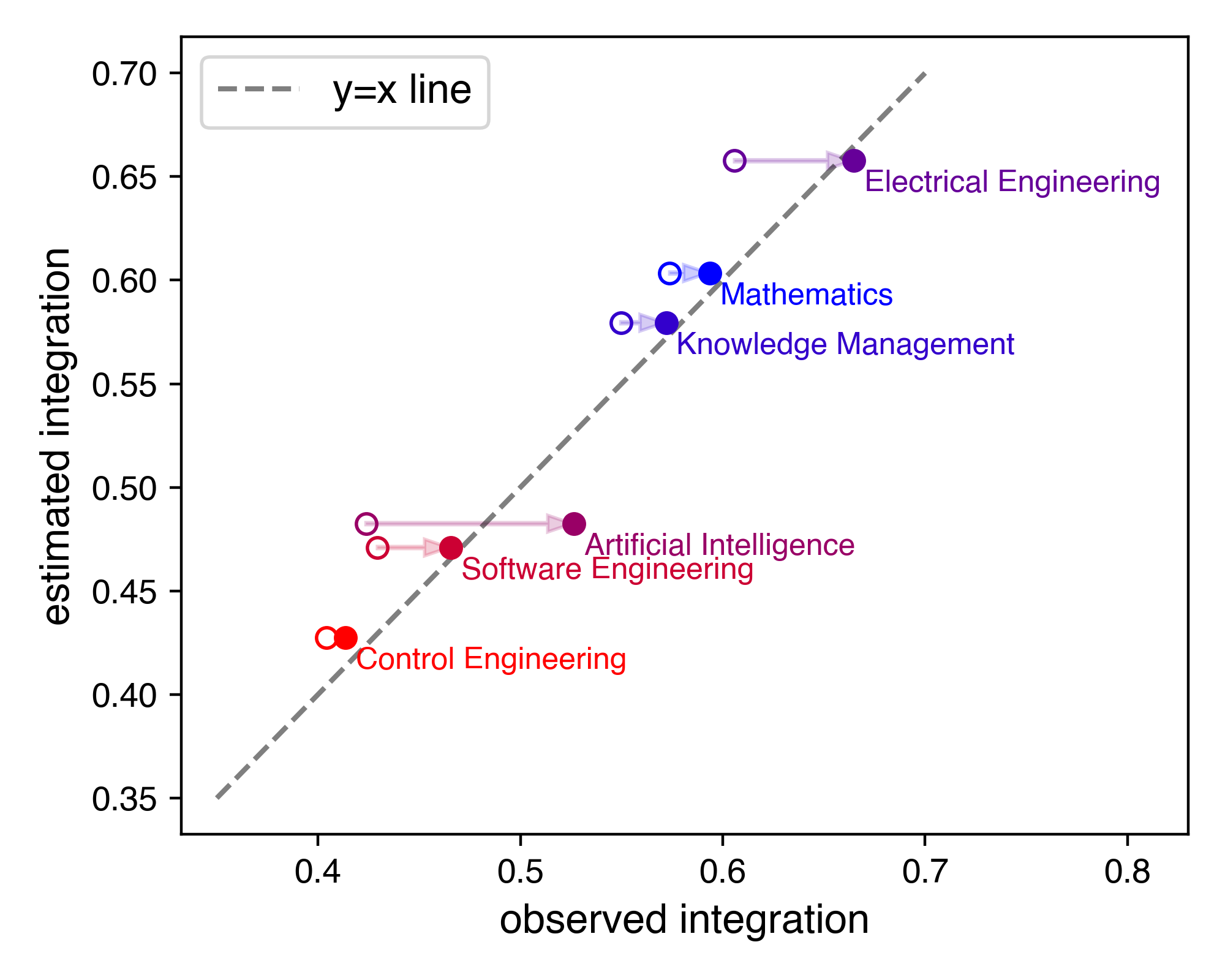
Figure 6. Estimated vs. observed integration. Theorem 3.1 is used to estimate network integration for different clusters. Empty and filled circles correspond to beginning and end year of the study, respectively.

Estimated and observed integration are very close except for one field.

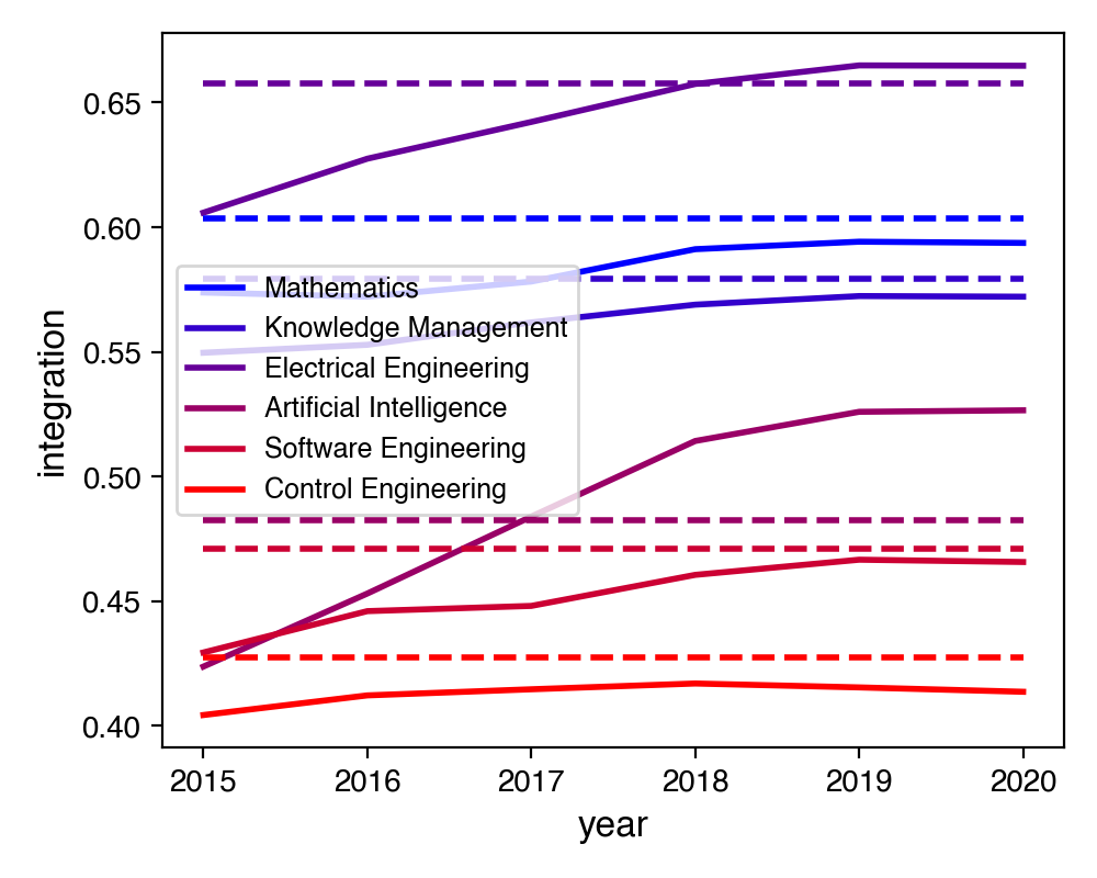
Figure 7. Convergence behavior of observed integration (solid) to estimated integration (dashed). With the exception of one field (Artificial Intelligence), network integration in other fields has converged to the predicted value.

Observed integration converges to the estimated integration by time except for one field.

5.3. Results of Citation Network Analysis

We use the obtained optimum parameters $\theta^{*}$ and Theorem 3.1 to estimate network integration in equilibrium. Figure 7 shows the estimated integration in equilibrium versus the observed integration. In this figure, empty and filled marks correspond to the starting year (2015) and final year (2020) respectively. With the exception of one cluster (Artificial Intelligence), different clusters consistently approach our estimated values from equilibrium. The convergence behavior is also depicted in Figure 7. These empirical insights show that even with the assumptions needed for Theorem 3.1, the theoretical insights closely match practice in this dataset. As we see from Figure 7, although clusters have various fields with different frequencies, their behavior in equilibrium is well-predicted from the theory with only a few parameters. Our empirical findings present further evidence that the Jackson-Rogers model explains citation network evolution. Finally, with estimated parameters, we find triadic closure to be responsible for $3$-$5\%$ of network integration. We do so by setting $N_{F}=0$ in Theorem 3.1, as a proxy for network integration without triadic closure.

6. Further Related Works

Homophily is a robust and prevalent process impacting network formation in many domains Lazarsfeldet al. (1954); McPhersonet al. (2001); Newman (2002). There is a long line of theoretical and empirical work exploring the effect of homophily on network formation, ranging from observational studies on large network data, to laboratory experiments, to analyses of theoretical models Adamic and Glance (2005); Donget al. (2017); Goereeet al. (2009).A main topic of focus has been the interaction between homophily and network segregation. For instance, Currariniet al. (2009); Henryet al. (2011) show that segregated networks emerge due to homophily. In related work, Kim and Altmann (2017) study the effect of homophily on the rich-get-richer phenomena. Empirical work has explored the effect of homophily on integration in settings like college campuses Mayer and Puller (2008). In related work to ours, Bramoullé et al. (2012) adapt the Jackson-Rogers model to the case with heterogeneous nodes. Their work primarily focuses on how each node’s likelihood to form links changes over time. In contrast, we consider a global measurement of integration, using the fraction of bichromatic edges.Triadic closure is another well-studied process in network formation dating back to the 1950s Kossinets andWatts (2006); Rapoport (1953). While there is a long line of work on the effect of triadic closure on network clustering, the interplay between homophily and triadic closure remains under-explored. In one complementary related work, Altenburger andUgander (2018) show that monophily—the presence of individuals with preference for attributes unrelated to their own—has a tendency to induce similarity among friends-of-friends. In contrast, we study the relationship of homophily and triadic closure, though some of the findings complement our observations.The closest work to ours is that by Asikainen et al. (2020), which explores the interaction of triadic closure and homophily. Here, we are similarly concerned with how these two phenomena interact in dynamic models. Asikainen et al. (2020) consider a model that also starts with an SBM and adds both triadic closure and random link rewiring. Both of these additions are influenced by choice homophily. Under this model, Asikainen et al. (2020) show that triadic closure amplifies the effects of homophily. We note, however, the model considered here already has the triadic closure step influenced by homophily. In our work, we make minimal adjustments to their model to further isolate the effects of triadic closure and find results consistent with the SBM and Jackson-Rogers models.Segregation in social networks can limit individuals’ ability to access information, resources, and opportunities, leading to the creation or exacerbation of disparities across groups. Research across various disciplines has modeled and measured the impact of segregation on social welfare including its impacts on access to information, economic development, educational outcomes, labor market outcomes, and social capital and support Banerjee et al. (2013); Calvo-Armengol andJackson (2004); Calvo-Armengol et al. (2009); Dasaratha (2017); DiMaggio andGarip (2011); Eagleet al. (2010); Jacksonet al. (2012)Recent work, such as by Avin et al. (2015) has proposed and studied models that explain how inequality and disparities in access to opportunity arise in certain settings.Our work has additional implications for network-based interventions both in on- and off-line settings. For instance, it is well-known thatbiases that may exist on online platforms such as Twitter and Task Rabbit may lead to inequalities between groups Nilizadeh et al. (2016); Hannák et al. (2017). These biases, amplified by recommendation algorithms, can impact how networks grow and evolve creating an algorithmic glass ceiling Biegaet al. (2018); Stoicaet al. (2018); Suet al. (2016); Biegaet al. (2018). In recent years, there has been interest by researchers in algorithmically-informed interventions that can help better diagnose and mitigate underlying patterns of inequality on platforms Abebe and Goldner (2018); Abebe et al. (2020). Focused on fairness in recommender systems, researchers have examined the effect of small interventions on the long-term health of the platform such as by mitigating segregation, improving interactions, and achieving other desirable societal objectives Ekstrand andWillemsen (2016); Guy (2015); Hutsonet al. (2018); Knijnenburg et al. (2016); Schnabel et al. (2018); Stoicaet al. (2018); Suet al. (2016). These studies have shown that the platform designer, by using small interventions when a user first joins, may be able to realize large gains on the platform health over time.

7. Discussion and Conclusion

In this work, we consider the effect of triadic closure on network segregation. Through analyses of different static and dynamic network formation models, we find that triadic closure has the effect of increasing network integration, indicating that it may be a process that counteracts homophily in network formation.We find it striking that such a tension should exist between two such well-studied social processes as homophily and triadic closure. In addition to the theoretical and empirical results tackled in this work, we believe this counter-intuitive result about the relationship between homophily and triadic closure points to a rich and under-explored phenomenon about their interaction.These results also open up questions related to other measurements of network health, such as network expansion and distribution of network centralities. Each of these points to challenging analytic questions. Empirically, it would also be interesting to shed light on what types of social and information networks tend to exhibit a stronger relationship between triadic closure and homophily.Finally, the interventions presented in this work point to a broader set of theoretical and empirical questions. For instance, it would be interesting to estimate the various network parameters and compare the effect of nudges across different distributions of values. Furthermore, such interventions are often costly to the designeror may incur social cost, leading to a set of optimization questions where the designer must trade off these costswith utility gained from network integration.We thank Sera Linardi, Emma Forman Ling, Irene Lo, Ashudeep Singh, Ana-Andreea Stoica, Sam Taggart, Bryan Wilder, Angela Zhou, and members of the MD4SG Working Group on Inequality for helpful discussions throughout the evolution of this work. We especially thank Emma Forman Ling for numerous discussions and pointers to the citation network. We additionally thank the reviewers, area chairs, track chairs, and program chairs of EC ’22 for their insightful feedback.

Appendix A Additional Statements and Proofs

Lemma A.1.

For any $\text{SBM}(p,q)$ network $G$ with $K\geq 2$ types each consisting of $n_{k}$ nodes ($k\in[K]$), the expected number of monochromatic edges is

$$e_{m}=\sum_{k\in[K]}{n_{k}\choose 2}p=\frac{1}{2}p\sum_{k}n_{k}^{2}+O(n),$$

and the expected number of bichromatic edges is

$$e_{b}=\frac{1}{2}\sum_{k\in[K]}\sum_{l\in[K],l\neq k}n_{k}n_{l}q=\frac{1}{2}q(n^{2}-\sum_{k}n_{k}^{2})+O(n),$$ (31)

where $n=\sum_{k}n_{k}$. Further, the expected number of monochromatic missing edges is

$$o_{m}=\sum_{k\in[K]}{n_{k}\choose 2}(1-p)=\frac{1}{2}(1-p)\sum_{k}n_{k}^{2}+O(n),$$

and the expected number of bichromatic missing edges is

$$o_{b}=\frac{1}{2}\sum_{k\in[K]}\sum_{l\in[K],l\neq k}n_{k}n_{l}(1-q)=\frac{1}{2}(1-q)\big{(}n^{2}-\sum_{k}n_{k}^{2}\big{)}+O(n),$$ (32)

where we call an edge $(i,j)$ a missing edge if $i$ and $j$ are not connected in $G$.

Proof.

To find $e_{m}$ ($o_{m}$), we sum the number of unordered pairs from each group times the probability they are connected (not connected). To find $e_{b}$ ($o_{b}$), we count the number of bichromatic pairs times the probability they are connected (not connected) times $\frac{1}{2}$ to compensate for repeated counting.∎

Lemma A.2.

For the same network as Lemma A.1, the expected number of monochromatic wedges is

$$w_{m} =\sum_{k\in[K]}{n_{k}\choose 2}(n_{k}-2)p^{2}(1-p)+\sum_{k\in[K]}{n_{k}\choose 2}(n-n_{k})q^{2}(1-p)$$

$$=\frac{1}{2}p^{2}(1-p)\sum_{k}n_{k}^{3}+\frac{1}{2}q^{2}(1-p)\big{(}n\sum_{k}n_{k}^{2}-\sum_{k}n_{k}^{3}\big{)}+O(n^{2}),$$ (33)

and the expected number of bichromatic wedges is

$$w_{b} =\sum_{k\in[K]}\sum_{l\in[K],l\neq k}n_{k}(n_{k}-1)n_{l}pq(1-q)+\sum_{k\in[K]}\sum_{l\in[K],l\neq k}\frac{1}{2}n_{k}n_{l}(n-n_{k}-n_{l})q^{2}(1-q)$$

$$=pq(1-q)\big{(}n\sum_{k}n_{k}^{2}-\sum_{k}n_{k}^{3}\big{)}+\frac{1}{2}q^{2}(1-q)\big{(}n^{3}+2\sum_{k}n_{k}^{3}-3n\sum_{k}n_{k}^{2}\big{)}+O(n^{2})$$ (34)

Proof.

For a wedge $i\text{---}j\text{---}k$, the first term of $w_{m}$ is the expected number of wedges such that $type(i)=type(j)=type(k)$. The second term of $w_{m}$ corresponds to the case $type(i)=type(k)\neq type(j)$. The first term of $w_{b}$ is the expected number of wedges such that $type(i)=type(j)\neq type(k)$. The second term of $w_{b}$ corresponds to the case where $i$, $j$, and $k$ are all from different types.∎

Lemma A.3.

For any set of $\{n_{1},n_{2},\cdots,n_{K}|n_{i}\in\mathbb{R}^{+}\}$, following inequalities hold:

1. $n^{2}\geq m_{2}$

2. $nm_{2}\geq m_{3}$

3. $nm_{3}\geq m_{2}^{2}$

4. $2m_{2}^{2}\geq nm_{3}$

5. $2nm_{2}^{2}\geq n^{2}m_{3}+m_{2}m_{3}$,

where $n=\sum_{k\in[K]}n_{k}$ and $m_{i}=\sum_{k\in[K]}n_{k}^{i}$.

Proof.

We start by the first inequality and use the results to that point in proving each inequality.

1. $$n^{2}-m_{2} =\sum_{i,j}n_{i}n_{j}-\sum_{j}n_{j}^{2}$$

   $$=\sum_{i\neq j}n_{i}n_{j}\geq 0.$$

2. $$nm_{2}-m_{3} =\sum_{i,j}n_{i}n_{j}^{2}-\sum_{j}n_{j}^{3}$$

   $$=\sum_{i\neq j}n_{i}n_{j}^{2}\geq 0.$$

3. $$nm_{3}-m_{2}^{2} =\sum_{i,j}n_{i}n_{j}^{3}-n_{i}^{2}n_{j}^{2}$$

   $$=\sum_{i\neq j}n_{i}n_{j}^{3}+n_{j}n_{i}^{3}-2n_{i}^{2}n_{j}^{2}$$

   $$=\sum_{i\neq j}n_{i}n_{j}(n_{i}-n_{j})^{2}\geq 0.$$

4. $$2m_{2}^{2}-nm_{3} =\sum_{i,j}2n_{i}^{2}n_{j}^{2}-n_{i}n_{j}^{3}$$

   $$=\sum_{i\neq j}n_{i}^{4}+n_{j}^{4}+4n_{i}^{2}n_{j}^{2}-n_{i}n_{j}^{3}-n_{j}n_{i}^{3}$$

   $$=\sum_{i\neq j}(n_{i}^{2}+n_{j}^{2})^{2}-n_{i}n_{j}(n_{i}-n_{j})^{2}.$$

   As $n_{i},n_{j}\geq 0$, $n_{i}^{2}+n_{j}^{2}\geq(\max(n_{i},n_{j}))^{2}\geq n_{i}n_{j}$ and $n_{i}^{2}+n_{j}^{2}\geq(\max(n_{i},n_{j}))^{2}\geq(n_{i}-n_{j})^{2}$. So, $(n_{i}^{2}+n_{j}^{2})^{2}\geq n_{i}n_{j}(n_{i}-n_{j})^{2}$, which gives $2m_{2}^{2}-nm_{3}\geq 0$.

5. $$2nm_{2}^{2}-n^{2}m_{3}-m_{2}m_{3} =(\sum_{i,j}2n_{i}^{2}n_{j}^{2}-n_{i}n_{j}^{2})n-\sum_{i,j}n_{i}^{2}n_{j}^{3}$$

   $$=\sum_{i\neq j}(n_{i}^{4}+n_{j}^{4}+4n_{i}^{2}n_{j}^{2}-n_{i}n_{j}^{3}-n_{j}n_{i}^{3})n-\sum_{i\neq j}n_{i}^{5}+n_{j}^{5}+n_{i}^{2}n_{j}^{3}+n_{j}^{2}n_{i}^{3}$$

   $$=\sum_{i\neq j}((n_{i}^{2}+n_{j}^{2})^{2}-n_{i}n_{j}(n_{i}-n_{j})^{2})(n-n_{i}-n_{j})$$

   $$+\sum_{i\neq j}(n_{i}^{4}+n_{j}^{4}+4n_{i}^{2}n_{j}^{2}-n_{i}n_{j}^{3}-n_{j}n_{i}^{3})(n_{i}+n_{j})-n_{i}^{5}+n_{j}^{5}+n_{i}^{2}n_{j}^{3}+n_{j}^{2}n_{i}^{3}$$

   $$\geq\sum_{i\neq j}(n_{i}^{4}+n_{j}^{4}+4n_{i}^{2}n_{j}^{2}-n_{i}n_{j}^{3}-n_{j}n_{i}^{3})(n_{i}+n_{j})-(n_{i}^{5}+n_{j}^{5}+n_{i}^{2}n_{j}^{3}+n_{j}^{2}n_{i}^{3})$$

   $$=\sum_{i\neq k}2n_{i}^{2}n_{j}^{3}+2n_{j}^{2}n_{i}^{2}\geq 0.$$

   Here we used $(n_{i}^{2}+n_{j}^{2})^{2}-n_{i}n_{j}(n_{i}-n_{j})^{2}\geq 0$ from the proof of the previous part.

∎

Lemma A.4.

Let ${\bm{A}}$ be a $K\times K$ real symmetric matrix such that

$$[{\bm{A}}]_{i,j}=\begin{cases}c&i=j\\ \frac{1}{K-1}(1-c)&o.w.\end{cases}.$$ (35)

Then, ${\bm{A}}$ has $K$ real eignvalues:

$$d_{i}=\begin{cases}1&i=1\\ \frac{Kc-1}{K-1}&1<i\leq K\end{cases},$$ (36)

with corresponding eigenvectors:

$$[{\bm{v}}_{1}]_{j} =1$$

$$\text{For $i\geq 2$: }[{\bm{v}}_{i}]_{j} =\begin{cases}1&j=1\\ -1&j=i\\ 0&o.w.\end{cases}.$$ (37)

Proof.

For $i=1$:

$$[{\bm{A}}{\bm{v}}_{1}]_{j}=1=d_{1}[{\bm{v}}_{1}]_{j}.$$ (38)

For $1<i\leq K$:

$$[{\bm{A}}{\bm{v}}_{i}]_{j}=\begin{cases}\frac{Kc-1}{K-1}&j=1\\ -\frac{Kc-1}{K-1}&j=i\\ 0&o.w.\end{cases}=d_{i}[{\bm{v}}_{1}]_{j}.$$ (39)

∎

Lemma A.5.

The inverse of the $K\times K$ matrix ${\bm{V}}$ defined by

$$[{\bm{V}}]_{i,j}=\begin{cases}1&i=1\text{ or }j=1\\ -1&i=j>1\\ 0&o.w.\end{cases}$$ (40)

is

$$[{\bm{V}}^{-1}]_{i,j}=\begin{cases}-\frac{K-1}{K}&i=j>1\\ \frac{1}{K}&o.w.\end{cases}.$$ (41)

Proof.

$$[{\bm{V}}{\bm{V}}^{-1}]_{i,j}=\begin{cases}1&i=j=1\\ \frac{1}{K}+\frac{K-1}{K}=1&i=j>1\\ 0&o.w.\end{cases}.$$ (42)

∎

Appendix B Simulations

First of all, we investigate stochastic block models through simulation. Specifically, we test Theorem 2.4 as Theorems 2.1 and 2.2 can be seen as special cases of this theorem for $\gamma=0$ and $\gamma\rightarrow\infty$, respectively. From Theorem 2.4 we expect triadic closure to have positive relative effect when $u(\gamma)>\frac{p}{q}>l(\gamma)$. To test this theorem, we have simulated a stochastic block model consisting of $K$ groups, where group $k$ has $n_{k}=10\,\lambda^{k}$ members. We use various values of $\frac{p}{q}$ and $\lambda$ in simulations. Figures 9 and 9 show the theoretical and simulated results together. Each mark on the figures shows specific values of $\frac{p}{q}$ and $\gamma$ that triadic closure has had a positive relative effect on average. One can see despite having small networks, Theorem 2.4 well predicts the effect both for balanced and unbalanced networks.

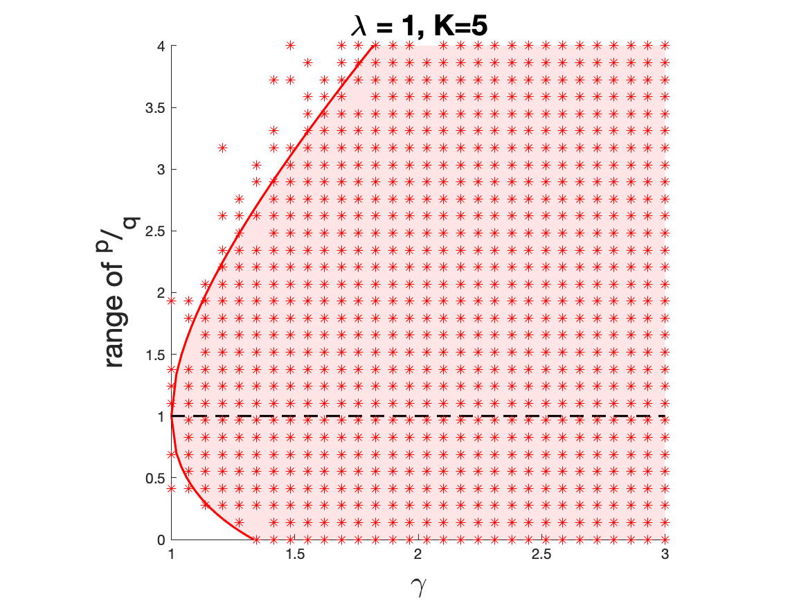
Figure 8. $u(\gamma)$ and $l(\gamma)$ for balanced groups. The shaded area is obtained by theory. Marks show positive relative effects in simulations.

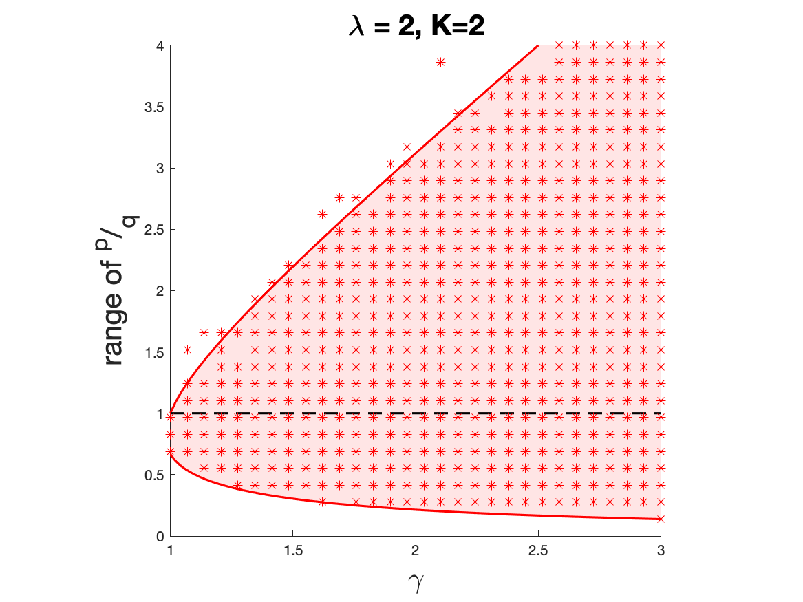
Figure 9. $u(\gamma)$ and $l(\gamma)$ for unbalanced groups. The shaded area is obtained by theory. Marks show positive relative effects in simulations.

Next, we study the Jackson-Rogers model’s convergence through simulations. Figure 11 shows network integration of a dynamic graph consisting of two groups evolving with the Jackson-Rogers model. The dashed lines show the integration in equilibrium predicted by Theorem 3.1. The solid and dotted lines show the average integration of repeated simulations for balanced and unbalanced networks. To show that behavior in equilibrium is independent of the initial network, we have run simulations for two cases: a completely segregated initial network and a fully connected initial network. It seems Theorem 3.1 can robustly predict the network’s behavior for various model parameters, regardless of the initial network and distribution of groups. Further, Figure 11 shows the residual to equilibrium on a logarithmic scale. The dashed lines correspond to the convergence rate $O(t^{-\frac{N_{S}+N_{D}}{N}})$. One can see the proposed upper bound on the convergence rate also matches the behavior of the network in simulations.

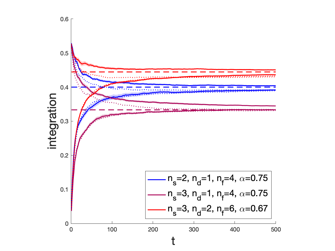
Figure 10. Convergence of a Jackson-Rogers network. Dashed lines show predicted behavior in equilibrium by Theorem 3.1.

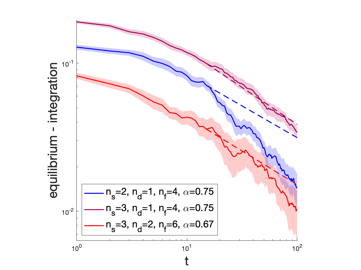
Figure 11. The residual to reach the predicted equilibrium. Dashed lines show predicted upper bound on the convergence rate.

References

- Abebe et al. (2020) Rediet Abebe, SolonBarocas, Jon Kleinberg, Karen Levy,Manish Raghavan, and David G Robinson.2020. Roles for computing in social change. InProceedings of the 2020 Conference on Fairness,Accountability, and Transparency. 252–260.
- Abebe and Goldner (2018) Rediet Abebe and KiraGoldner. 2018. Mechanism design for social good. AI Matters 4,3 (2018), 27–34.
- Adamic and Glance (2005) Lada A Adamic andNatalie Glance. 2005. The political blogosphere and the 2004 US election:divided they blog. In Proceedings of the 3rdinternational workshop on Link discovery. 36–43.
- Altenburger andUgander (2018) Kristen M Altenburger andJohan Ugander. 2018. Monophily in social networks introduces similarityamong friends-of-friends. Nature human behaviour 2,4 (2018), 284.
- Asikainen et al. (2020) Aili Asikainen, GerardoIñiguez, Javier Ureña-Carrión,Kimmo Kaski, and Mikko Kivelä.2020. Cumulative effects of triadic closure and homophilyin social networks. Science Advances 6,19 (2020), eaax7310.
- Avin et al. (2015) Chen Avin, BarbaraKeller, Zvi Lotker, Claire Mathieu,David Peleg, and Yvonne-Anne Pignolet.2015. Homophily and the glass ceiling effect in socialnetworks. In Proceedings of the 2015 conference oninnovations in theoretical computer science. 41–50.
- Banerjee et al. (2013) Abhijit Banerjee, Arun GChandrasekhar, Esther Duflo, andMatthew O Jackson. 2013. The diffusion of microfinance. Science 341,6144 (2013).
- Biegaet al. (2018) Asia J Biega, Krishna PGummadi, and Gerhard Weikum.2018. Equity of Attention: Amortizing Individual Fairnessin Rankings. arXiv preprint arXiv:1805.01788(2018).
- Bramoullé et al. (2012) Yann Bramoullé, SergioCurrarini, Matthew O Jackson, Paolo Pin,and Brian W Rogers. 2012. Homophily and long-run integration in socialnetworks. Journal of Economic Theory147, 5 (2012).
- Calvo-Armengol andJackson (2004) Antoni Calvo-Armengol andMatthew O Jackson. 2004. The effects of social networks on employment andinequality. American Economic Review94, 3 (2004).
- Calvo-Armengol et al. (2009) Antoni Calvo-Armengol,Eleonora Patacchini, and Yves Zenou.2009. Peer effects and social networks in education. The Review of Economic Studies76, 4 (2009).
- Chung andRadcliffe (2011) Fan Chung and MaryRadcliffe. 2011. On the spectra of general random graphs. the electronic journal of combinatorics(2011), P215–P215.
- Currariniet al. (2009) Sergio Currarini,Matthew O Jackson, and Paolo Pin.2009. An economic model of friendship: Homophily,minorities, and segregation. Econometrica 77,4 (2009), 1003–1045.
- Dasaratha (2017) Krishna Dasaratha.2017. Distributions of Centrality on Networks. arXiv preprint arXiv:1709.10402(2017).
- Del Vicario et al. (2016) Michela Del Vicario,Gianna Vivaldo, Alessandro Bessi,Fabiana Zollo, Antonio Scala,Guido Caldarelli, and WalterQuattrociocchi. 2016. Echo chambers: Emotional contagion and grouppolarization on facebook. Scientific reports 6,1 (2016), 1–12.
- DiMaggio andGarip (2011) Paul DiMaggio and FilizGarip. 2011. How network externalities can exacerbate intergroupinequality. Amer. J. Sociology 116,6 (2011), 1887–1933.
- Donget al. (2017) Yuxiao Dong, Reid AJohnson, Jian Xu, and Nitesh VChawla. 2017. Structural diversity and homophily: A study acrossmore than one hundred big networks. In Proceedingsof the 23rd ACM SIGKDD International Conference on Knowledge Discovery andData Mining. 807–816.
- Eagleet al. (2010) Nathan Eagle, MichaelMacy, and Rob Claxton. 2010. Network diversity and economic development. Science 328,5981 (2010), 1029–1031.
- Easley andKleinberg (2010) David Easley and JonKleinberg. 2010. Networks, Crowds, and Markets: Reasoningabout a Highly Connected World. Cambridge University Press. https://doi.org/10.1017/CBO9780511761942
- Ekstrand andWillemsen (2016) Michael D Ekstrand andMartijn C Willemsen. 2016. Behaviorism is not enough: better recommendationsthrough listening to users. In Proceedings of the10th ACM Conference on Recommender Systems. ACM, 221–224.
- Goereeet al. (2009) Jacob K Goeree, ArnoRiedl, and Aljaž Ule.2009. In search of stars: Network formation amongheterogeneous agents. Games and Economic Behavior67, 2 (2009).
- Granovetter (1977) Mark S Granovetter.1977. The strength of weak ties. In Social networks.Elsevier, 347–367.
- Guy (2015) Ido Guy. 2015. Social recommender systems. In Recommender Systems Handbook.Springer, 511–543.
- Hannák et al. (2017) Anikó Hannák,Claudia Wagner, David Garcia,Alan Mislove, Markus Strohmaier, andChristo Wilson. 2017. Bias in online freelance marketplaces: Evidencefrom taskrabbit and fiverr. In Proceedings of the2017 ACM conference on computer supported cooperative work and socialcomputing. 1914–1933.
- Henryet al. (2011) Adam Douglas Henry,Paweł Prałat, and Cun-QuanZhang. 2011. Emergence of segregation in evolving socialnetworks. Proc. of the National Academy of Sciences108, 21 (2011).
- Hutsonet al. (2018) Jevan Hutson, Jessie GTaft, Solon Barocas, and Karen Levy.2018. Debiasing Desire: Addressing Bias & Discriminationon Intimate Platforms. arXiv preprint arXiv:1809.01563(2018).
- Jacksonet al. (2012) Matthew O. Jackson, TomasRodriguez-Barraquer, and Xu Tan.2012. Social Capital and Social Quilts: Network Patternsof Favor Exchange. American Economic Review102, 5 (May2012). https://doi.org/10.1257/aer.102.5.1857
- Jackson andRogers (2007) Matthew O. Jackson andBrian W. Rogers. 2007. Meeting Strangers and Friends of Friends: HowRandom Are Social Networks? American Economic Review97, 3 (June2007), 890–915. https://doi.org/10.1257/aer.97.3.890
- Kim and Altmann (2017) Kibae Kim and JörnAltmann. 2017. Effect of homophily on network formation. Comm. in Nonlinear Science and NumericalSimulation 44 (2017).
- Knijnenburg et al. (2016) Bart P Knijnenburg,Saadhika Sivakumar, and DariciaWilkinson. 2016. Recommender systems for self-actualization. InProceedings of the 10th ACM Conference onRecommender Systems. ACM, 11–14.
- Kossinets andWatts (2006) Gueorgi Kossinets andDuncan J Watts. 2006. Empirical analysis of an evolving social network. science 311,5757 (2006), 88–90.
- Kossinets andWatts (2009) Gueorgi Kossinets andDuncan J Watts. 2009. Origins of homophily in an evolving socialnetwork. American journal of sociology115, 2 (2009),405–450.
- Lazarsfeldet al. (1954) Paul F Lazarsfeld,Robert K Merton, et al.1954. Friendship as a social process: A substantive andmethodological analysis. Freedom and control in modern society18, 1 (1954),18–66.
- Mayer and Puller (2008) Adalbert Mayer andSteven L Puller. 2008. The old boy (and girl) network: Social networkformation on university campuses. Journal of Public Economics92, 1-2 (2008).
- McPherson andSmith-Lovin (1987) J Miller McPherson andLynn Smith-Lovin. 1987. Homophily in voluntary organizations: Statusdistance and the composition of face-to-face groups. American sociological review(1987), 370–379.
- McPhersonet al. (2001) Miller McPherson, LynnSmith-Lovin, and James M Cook.2001. Birds of a feather: Homophily in social networks. Annual review of sociology27, 1 (2001).
- Newman (2002) Mark EJ Newman.2002. Assortative mixing in networks. Physical review letters89, 20 (2002),208701.
- Nilizadeh et al. (2016) Shirin Nilizadeh, AnneGroggel, Peter Lista, Srijita Das,Yong-Yeol Ahn, Apu Kapadia, andFabio Rojas. 2016. Twitter’s glass ceiling: The effect of perceivedgender on online visibility. In Proceedings of theInternational AAAI Conference on Web and Social Media,Vol. 10. 289–298.
- Rapoport (1953) Anatol Rapoport.1953. Spread of information through a population withsocio-structural bias: I. Assumption of transitivity. The bulletin of mathematical biophysics15, 4 (1953),523–533.
- Schnabel et al. (2018) Tobias Schnabel, Paul NBennett, Susan T Dumais, and ThorstenJoachims. 2018. Short-term satisfaction and long-term coverage:Understanding how users tolerate algorithmic exploration. InProceedings of the Eleventh ACM InternationalConference on Web Search and Data Mining. ACM, 513–521.
- Shrumet al. (1988) Wesley Shrum, Neil HCheek Jr, and Saundra MacD.1988. Friendship in school: Gender and racial homophily. Sociology of Education(1988), 227–239.
- Stoicaet al. (2018) Ana-Andreea Stoica,Christopher Riederer, and AugustinChaintreau. 2018. Algorithmic Glass Ceiling in Social Networks: Theeffects of social recommendations on network diversity. InProceedings of the 2018 World Wide WebConference. 923–932.
- Suet al. (2016) Jessica Su, AneeshSharma, and Sharad Goel.2016. The effect of recommendations on networkstructure. In Proceedings of the 25thinternational conference on World Wide Web. 1157–1167.
- Tanget al. (2008) Jie Tang, Jing Zhang,Limin Yao, Juanzi Li, LiZhang, and Zhong Su. 2008. ArnetMiner: Extraction and Mining of AcademicSocial Networks. In KDD’08.990–998.
- Tóth et al. (2019) Gergő Tóth,Johannes Wachs, Riccardo Di Clemente,Ákos Jakobi, Bence Ságvári,János Kertész, and BalázsLengyel. 2019. Inequality is rising where social networksegregation interacts with urban topology. arXiv preprint arXiv:1909.11414(2019).
- Zeltzer (2020) Dan Zeltzer.2020. Gender homophily in referral networks: Consequencesfor the medicare physician earnings gap. American Economic Journal: AppliedEconomics 12, 2 (2020),169–97.