A Semidefinite Relaxation for Sums of Heterogeneous Quadratic Forms on the Stiefel Manifold

Abstract

We study the maximization of sums of heterogeneous quadratic forms over the Stiefel manifold, a nonconvex problem that arises in several modern signal processing and machine learning applications such as heteroscedastic probabilistic principal component analysis (HPPCA). In this work, we derive a novel semidefinite program (SDP) relaxation and study a few of its theoretical properties. We prove a global optimality certificate for the original nonconvex problem via a dual certificate, which leads to a simple feasibility problem to certify global optimality of a candidate local solution on the Stiefel manifold. In addition, our relaxation reduces to an assignment linear program for jointly diagonalizable problems and is therefore known to be tight in that case. We generalize this result to show that it is also tight for close-to jointly diagonalizable problems, and we show that the HPPCA problem has this characteristic. Numerical results validate our global optimality certificate and sufficient conditions for when the SDP is tight in various problem settings.

1 Introduction

This paper studies the problem known in the literature as the maximization of sums of heterogeneous quadratic forms over the Stiefel manifold [17, 8, 41, 7]. Specifically, given $d\times d$ symmetric positive semidefinite (PSD) matrices $\mathbf{M}_{1},\ldots,\mathbf{M}_{k}\succeq 0$ for $k\leq d$, we wish to maximize the convex objective function $\sum_{i=1}^{k}\mathbf{u}_{i}^{\prime}\mathbf{M}_{i}\mathbf{u}_{i}$ over the nonconvex constraint that $\mathbf{U}=[\mathbf{u}_{1}\cdots\mathbf{u}_{k}]\in\mathbb{R}^{d\times k}$ has orthonormal columns:

(1) $$\max_{\mathbf{U}\in\text{St}(k,d)}\sum_{i=1}^{k}\mathbf{u}_{i}^{\prime}\mathbf{M}_{i}\mathbf{u}_{i},$$

where $\text{St}(k,d)=\{\mathbf{U}\in\mathbb{R}^{d\times k}:\mathbf{U}^{\prime}\mathbf{U}=\mathbf{I}_{k}\}$ denotes the Stiefel manifold. This problem arises in modern signal processing and machine learning applications like heteroscedastic probabilistic principal component analysis (HPPCA) [29], heterogeneous clutter in radar sensing [44], and robust sparse PCA [16]. Each of these applications involves learning a signal subspace for data possessing heterogeneous statistics.

In particular, HPPCA [29] models data collected from sources of varying quality with different additive noise variances, and estimates the best approximating low-dimensional subspace by maximizing the likelihood, providing superior estimation compared to standard PCA. Specifically, given $L$ data groups $[\mathbf{Y}_{1},\ldots,\mathbf{Y}_{L}]$ with $\mathbf{Y}_{\ell}\in\mathbb{R}^{d\times n_{\ell}}$, second-order statistics $\mathbf{A}_{\ell}:=\frac{1}{v_{\ell}}\mathbf{Y}_{\ell}\mathbf{Y}_{\ell}^{\prime}\succeq 0$ for $\ell\in[L]$, and known positive weights $w_{\ell,i}$ for $(\ell,i)\in[L]\times[k]$, a subproblem of HPPCA involves optimizing the sum of Brockett cost functions [2, Section 4.8] with respect to a $k$-dimensional orthonormal basis $\mathbf{U}$, and can be equivalently recast in the form Eq. 1 as follows:

(2) $$\max_{\mathbf{U}:\mathbf{U}^{\prime}\mathbf{U}=\mathbf{I}}\sum_{\ell=1}^{L}\operatorname{tr}(\mathbf{U}^{\prime}\mathbf{A}_{\ell}\mathbf{U}\mathbf{W}_{\ell})=\max_{\mathbf{U}:\mathbf{U}^{\prime}\mathbf{U}=\mathbf{I}}\sum_{\ell=1}^{L}\sum_{i=1}^{k}w_{\ell,i}\mathbf{u}_{i}^{\prime}\mathbf{A}_{\ell}\mathbf{u}_{i}=\max_{\mathbf{U}:\mathbf{U}^{\prime}\mathbf{U}=\mathbf{I}}\sum_{i=1}^{k}\mathbf{u}_{i}^{\prime}\mathbf{M}_{i}\mathbf{u}_{i},$$

where $\mathbf{W}_{\ell}:=\text{diag}(\{w_{\ell,i}\}_{i=1}^{k})$ for all $\ell$ and $\mathbf{M}_{i}:=\sum_{\ell=1}^{L}w_{\ell,i}\mathbf{A}_{\ell}$ for all $i$. Other sensing problems such as independent component analysis (ICA) [46] and approximate joint diagonalization (AJD) [38] also model data with heterogeneous statistics and optimize objective functions of a similar form, as we discuss in Section 3.

For (2), the case of a single Brockett cost function ($L=1$) has a known analytical solution obtained by the SVD or eigendecomposition [2, Section 4.8], whereas analytical solutions are not known for $L\geq 2$. Indeed, for $L\geq 2$ and general $\mathbf{A}_{\ell}$, few, if any, guarantees for optimal recovery exist except in special cases, such as when the constructed $\mathbf{M}_{i}$ commute [8]. Generally speaking, existing theory only gives restrictive sufficient conditions for global optimality that are typically difficult to check in practice; see [41], for example. Given that (1) is nontrivial and challenging in several ways—nonconvex due to the Stiefel manifold constraint, non-separable because of the weighted sum of objectives, and not readily solved by singular value or eigenvalue decomposition—many works apply iterative local solvers to (1).

However, given the nonconvexity of Eq. 1, these local approaches do not find a global maximum in general. An alternative approach is to relax problems such as (1) to a semidefinite program (SDP), allowing the use of standard convex solvers. While the SDP has stronger optimality guarantees, the challenge is then to derive conditions under which the SDP is tight, i.e., returns an optimal solution to the original nonconvex problem. SDP relaxations such as the “Fantope” [25, 36] exist for solving PCA-like problems, but to the best of our knowledge, no previous convex methods exist to solve (1).

The main contribution of this paper is a novel convex SDP relaxation of (1), whose constraint set is related to the Fantope but distinct. By studying this SDP and its optimality criteria, we derive sufficient conditions to certify the global optimality of a local stationary point, e.g., a candidate solution obtained from any iterative solver for the nonconvex problem. We then propose a straightforward method to certify global optimality by solving a much smaller SDP feasibility problem that scales favorably with the problem dimension. Our work also generalizes existing results for Eq. 1 with commuting matrices to the case with “almost commuting” matrices, showing that as long as the data matrices are within an open neighborhood of a commuting tuple of data matrices (to be defined precisely in Section 4.2), the SDP is tight and provably recovers an optimal solution of (1).

Notation

We use italic, boldface, upper case letters $\mathbf{A}$ to denote matrices, $\mathbf{v}$ to denote vectors, and $c$ for scalars. We denote the cone of $d\times d$-size symmetric positive semidefinite matrices as $\mathbb{S}^{d}_{+}$, and use $\mathbf{A}\succeq 0$ to denote an element $\mathbf{A}\in\mathbb{S}^{d}_{+}$. We denote the Hermitian transpose of a matrix as $\mathbf{A}^{\prime}$, the trace of a matrix as $\operatorname{tr}(\mathbf{A})$, and the inner product of matrices (with compatible inner dimensions) $\langle\mathbf{A},\mathbf{B}\rangle:=\operatorname{tr}(\mathbf{A}^{\prime}\mathbf{B})$. The spectral norm of a matrix is denoted by $\|\mathbf{A}\|$ and the Frobenius norm by $\|\mathbf{A}\|_{F}$. The identity matrix of size $d$ is denoted as $\mathbf{I}_{d}$. Notation $i\in[k]$ means $i=1,\dots,k$.

2 Semidefinite program relaxation

By relaxing the considered nonconvex problem Eq. 1 to a convex one, the well-established principles of convex optimization permit us to study when an optimal solution of the SDP relaxation recovers a global maximum of Eq. 1 and importantly, when a given local stationary point is a global maximum. After re-expressing the original problem using equivalent constraints, we lift the variables into the cone of PSD matrices, relax the nonconvex constraints to convex surrogates, and obtain an SDP.

First, we begin by slightly rewriting Eq. 1 and the Stiefel manifold constraints as

(3) $$\max_{\mathbf{u}_{1},\ldots,\mathbf{u}_{k}} \operatorname{tr}\left(\sum_{i=1}^{k}\mathbf{M}_{i}\mathbf{u}_{i}\mathbf{u}_{i}^{\prime}\right)\quad\text{s.t. }\operatorname{tr}\left(\mathbf{u}_{i}\mathbf{u}_{i}^{\prime}\right)=1\quad\forall i\in[k],\quad\operatorname{tr}\left(\mathbf{u}_{j}\mathbf{u}_{i}^{\prime}\right)=0\quad\forall i\neq j.$$

Letting $\mathbf{X}_{i}=\mathbf{u}_{i}\mathbf{u}_{i}^{\prime}\in\mathbb{R}^{d\times d}$, this is equivalent to the lifted problem:

(4) $$\begin{split}\max_{\mathbf{X}_{1},\ldots,\mathbf{X}_{k}}\operatorname{tr}\left(\sum_{i=1}^{k}\mathbf{M}_{i}\mathbf{X}_{i}\right)\quad\text{s.t.}&~{}\lambda_{j}\left(\sum_{i=1}^{k}\mathbf{X}_{i}\right)\in\{0,1\}\quad\forall j\in[d]\\ &\operatorname{tr}(\mathbf{X}_{i})=1,\quad{{\text{rank}}(\mathbf{X}_{i})=1},\quad\mathbf{X}_{i}\succcurlyeq 0\quad\forall i\in[k],\end{split}$$

where $\lambda_{j}(\cdot)$ indicates the $j$-th eigenvalue of its argument. Note that this problem is nonconvex due to the rank constraint and the constraint that the eigenvalues are binary. Similar to the relaxations in [47, 35], we relax the eigenvalue constraint in (4) to $0\preccurlyeq\sum_{i=1}^{k}\mathbf{X}_{i}\preccurlyeq\mathbf{I}\;$ and remove the rank constraint, which yields the SDP relaxation we consider throughout the remainder of this work:

(SDP-P) $$\begin{split}p^{*}=\min_{\mathbf{X}_{1},\ldots,\mathbf{X}_{k}}&\quad-\operatorname{tr}\left(\sum_{i=1}^{k}\mathbf{M}_{i}\mathbf{X}_{i}\right)\quad\\ &\text{s.t.}~{}\sum_{i=1}^{k}\mathbf{X}_{i}\preccurlyeq\mathbf{I},\quad\operatorname{tr}(\mathbf{X}_{i})=1,\quad\mathbf{X}_{i}\succcurlyeq 0\quad i=1,\dots,k.\end{split}$$

Note that $0\preccurlyeq\sum_{i=1}^{k}\mathbf{X}_{i}$ can be omitted since it is already satisfied when $\mathbf{X}_{i}\succcurlyeq 0$ for all $i$. The feasible set of (SDP-P) is closely related to the convex set found in [47, 35, 26] called the Fantope. The Fantope is the convex hull of all matrices $\mathbf{U}\mathbf{U}^{\prime}\in\mathbb{R}^{d\times d}$ such that $\mathbf{U}\in\mathbb{R}^{d\times k}$ and $\mathbf{U}^{\prime}\mathbf{U}=\mathbf{I}$ [25, 36]. Indeed, our relaxation can be viewed as providing a decomposition of the Fantope variable $\mathbf{X}$ into the sum $\mathbf{X}_{1}+\cdots+\mathbf{X}_{k}$ such that each $\mathbf{X}_{i}$ satisfies $\operatorname{tr}(\mathbf{X}_{i})=1$ and $0\preceq\mathbf{X}_{i}\preceq\mathbf{I}$. This decomposition allows (SDP-P) to capture the exact form of the objective function, which sums the individual terms $\operatorname{tr}(\mathbf{M}_{i}\mathbf{X}_{i})$. Precisely, the feasible set of (SDP-P) is a convex relaxation of the set $\left\{(\mathbf{u}_{1}\mathbf{u}_{1}^{\prime},\ldots,\mathbf{u}_{k}\mathbf{u}_{k}^{\prime}):\mathbf{U}^{\prime}\mathbf{U}=\mathbf{I}\right\}$. Naturally, one wonders whether our relaxation always solves the original nonconvex problem. We show in Appendix J that it does not, using a counter-example. Our work therefore studies this SDP in two ways: first, we provide a global optimality certificate; second, we study a class of “close-to jointly diagonalizable” problem instances, which includes the heteroscedastic PCA problem, and show that the SDP is tight for this class.

For dual variables $\mathbf{Z}_{i}\in\mathbb{S}_{+}^{d}$, $\mathbf{Y}\in\mathbb{S}_{+}^{d}$, $\bm{\nu}\in\mathbb{R}^{k}$, the dual of Eq. SDP-P (derived in Appendix F), which will play a central role in the theory of this paper, is

(SDP-D) $$d^{*}=\min_{\mathbf{Y},\mathbf{Z}_{i},\bm{\nu}} \operatorname{tr}(\mathbf{Y})+\sum_{i=1}^{k}\nu_{i}\quad\text{s.t. }\mathbf{Y}\succcurlyeq 0,\quad\mathbf{Y}=\mathbf{M}_{i}+\mathbf{Z}_{i}-\nu_{i}\mathbf{I},\quad\mathbf{Z}_{i}\succcurlyeq 0\quad\forall i\in[k].$$

Since the constraint set of Eq. SDP-P is closed and bounded with non-empty interior, and strong duality holds by Lemma 2.4 below, there exists an optimal primal solution to Eq. SDP-P and optimal dual solution to Eq. SDP-D.

Definition 2.1 (Rank-one property (ROP)).

A feasible solution to Eq. SDP-P is said to have the rank-one property if $\mathbf{X}_{1},\ldots,\mathbf{X}_{k}$ are all rank-one.

We note that if a feasible solution has the rank-one property, the first singular vectors of the $\mathbf{X}_{i}$ are necessarily mutually orthogonal, and $\sum_{i}\mathbf{X}_{i}$ is a rank-$k$ projection matrix, due to the constraint $\sum_{i}\mathbf{X}_{i}\preccurlyeq\mathbf{I}$.

Our theoretical results require the following lemmas, whose proofs can be found in Appendix A.

Lemma 2.2.

Assume all $\mathbf{M}_{i}$ are PSD. Then all $\nu_{i}\geq 0$ at optimality.

Lemma 2.3.

If the optimal dual variables $\mathbf{Z}_{i}$ for $i=1,\ldots,k$ each have rank $d-1$, the optimal solution $\mathbf{X}^{*}:=(\mathbf{X}^{*}_{1},\ldots,\mathbf{X}^{*}_{k})$ has the rank-one property.

Lemma 2.4.

Strong duality holds for the SDP relaxation with primal (SDP-P) and dual (SDP-D).

Lemma 2.5.

The solution to the SDP relaxation in (SDP-P) is the optimal solution to the original nonconvex problem in (1) (equivalently (4)) if and only if the optimal $\mathbf{X}^{*}:=(\mathbf{X}^{*}_{1},\ldots,\mathbf{X}^{*}_{k})$ has the rank-one property.

3 Related work

There are a few important related works on the objective in Eq. 1, as well as many more than can be reviewed here, including ones on eigenvalue/eigenvector problems and their variations, low-rank SDPs, and nonconvex quadratics where $\mathbf{M}_{i}$ are not PSD. For the curious reader, Section D in the supplement provides a more extensive related work section. Here, we focus on the works most directly related to Eq. 1.

The papers [8, 41, 7] previously investigated the sum of heterogeneous quadratic forms in Eq. 1. The work in [8] only studied the structure of this problem when the matrices $\mathbf{M}_{i}$ were commuting. The work in [41] derived sufficient second-order global optimality conditions, but these conditions are difficult to check in general and, for example, do not seem to hold for the heteroscedastic PCA problem. Works such as [30] and [37] consider a very similar problem to (2), but without the eigenvalue constraint in (4), making their SDP a rank-constrained separable SDP; see also [35, Section 4.3]. Pataki [37] studied upper bounds on the rank of optimal solutions of general SDPs, but in the case of Eq. SDP-P, since our problem introduces the additional constraint summing the $\mathbf{X}_{i}$, Pataki’s bounds do not guarantee rank-one, or even low-rank, optimal solutions.

Recent works have also studied convex relaxations of PCA and other low-rank subspace problems that seek to bound the eigenvalues of a single matrix [47, 45, 50], rather than the sum of multiple matrices as in our setting. The works in [11, 40] show nonconvex Burer–Monteiro factorizations [19] to solve low-rank SDPs without orthogonality constraints have no spurious local minima and that approximate second-order stationary points are approximate global optima. Other works have studied algorithms to optimize the nonconvex problem, like those in [16, 15, 44, 14, 29], using minorize-maximize or Riemannian gradient ascent algorithms, which do not come with global optimality guarantees. Our problem also has interesting connections to approximate joint diagonalization (AJD), which is well-studied and often applied to blind source separation or independent component analysis (ICA) problems [46, 10, 32, 3, 43]. See Appendix D of the supplement for further details.

4 Theoretical Results

4.1 Dual certificate of the SDP

In practical settings for high-dimensional data, a variety of iterative local methods are often applied to solve nonconvex problems over the Stiefel manifold, from gradient ascent by geodesics [2, 23, 1] to majorization-minimization (MM) algorithms, where [16] applied MM methods to solve Eq. 1 with guarantees of convergence to a stationary point. While the computational complexity and memory requirements of these solvers scale well, their obtained solutions lack any global optimality guarantees. We seek to fill this gap by proposing a check for global optimality of a local solution.

By Lemma 2.5, an optimal solution of Eq. SDP-P with rank-one matrices $\mathbf{X}_{i}$ globally solves the original nonconvex problem Eq. 1. In this section, given a candidate stationary point $\bar{\mathbf{U}}=[\bar{\mathbf{u}}_{1}\cdots\bar{\mathbf{u}}_{k}]\in\text{St}(k,d)$ to Eq. 1, we investigate conditions guaranteeing that the rank-one matrices $\bar{\mathbf{X}}_{i}=\bar{\mathbf{u}}_{i}\bar{\mathbf{u}}_{i}^{\prime}$, which are feasible for Eq. SDP-P, in fact comprise an optimal solution of Eq. SDP-P, implying that $\bar{\mathbf{U}}$ optimizes Eq. 1. Similar to [49, 24] for Fantope problems, our results yield a dual SDP certificate to verify the primal optimality of the candidates $\bar{\mathbf{X}}_{1},\ldots,\bar{\mathbf{X}}_{k}$ constructed from a local solution $\bar{\mathbf{U}}$. We show our certificate scales favorably in computation compared to the full SDP, with the most complicated computations of our algorithm requiring us to solve a feasibility problem in $k$ variables with several $d\times d$-size linear matrix inequalities (LMI).

Theorem 4.6.

Let $\bar{\mathbf{U}}\in\textup{St}(k,d)$ be a second-order stationary point of Eq. 1, and let $\bar{\bm{\Lambda}}=\sum_{i=1}^{k}\bar{\mathbf{U}}^{\prime}\mathbf{M}_{i}\bar{\mathbf{U}}\mathbf{E}_{i}$, where $\mathbf{E}_{i}\triangleq\mathbf{e}_{i}\mathbf{e}_{i}^{\prime}$ and $\mathbf{e}_{i}$ is the $i^{\text{th}}$ standard basis vector in $\mathbb{R}^{k}$, and $\mathbf{M}_{i}\succeq 0$ for all $i\in[k]$. If there exist $\bar{\bm{\nu}}=[\bar{\nu}_{1}\cdots\bar{\nu}_{k}]\in\mathbb{R}^{k}_{+}$ such that

(5) $$\begin{split}\bar{\mathbf{U}}(\bar{\bm{\Lambda}}-\mathbf{D}_{\bar{\bm{\nu}}})\bar{\mathbf{U}}^{\prime}+\bar{\nu}_{i}\mathbf{I}-\mathbf{M}_{i}&\succeq 0\quad\forall i=1,\ldots,k\\ \bar{\bm{\Lambda}}-\mathbf{D}_{\bar{\bm{\nu}}}&\succeq 0,\end{split}$$

where $\mathbf{D}_{\bar{\bm{\nu}}}:=\text{diag}(\bar{\nu}_{1},\ldots,\bar{\nu}_{k})$, then $\bar{\mathbf{U}}$ is a globally optimal solution to the original nonconvex problem Eq. 1.

In light of Theorem 4.6, to test whether a candidate stationary point $\bar{\mathbf{U}}$ is globally optimal, we simply assess whether system Eq. 5 is feasible using an LMI solver. If it is indeed feasible, then $\bar{\mathbf{U}}$ is globally optimal. On the other hand, if Eq. 5 is infeasible, it indicates one of two things: 1) The SDP does not return tight, rank-one solutions $\bar{\mathbf{X}}_{i}$, and the SDP strictly upper bounds the original problem on the Stiefel manifold. The candidate stationary point $\bar{\mathbf{U}}$ may or may not be globally optimal to the original nonconvex problem. 2) The SDP is tight, but the candidate stationary point $\bar{\mathbf{U}}$ is a suboptimal local solution. The proof, found in Appendix B, constructs dual variables and verifies the KKT conditions. Section N also describes an extension of the certificate to the sum of Brocketts with additive linear terms.

Arithmetic complexity

While SDP relaxations of nonconvex optimization problems can provide strong provable guarantees, their practicality can be limited by the time and space required to solve them, particularly when using off-the-shelf interior-point solvers, which in our case require $\mathcal{O}(d^{3})$ [5] storage and floating point operations (flops) per iteration of Eq. SDP-D. The proposed global certificate in Eq. 5 significantly reduces the number of variables from $\mathcal{O}(d^{2})$ in Eq. SDP-D (upon eliminating the variables $\mathbf{Z}_{i}$) to merely $k$ variables in Eq. 5. Using [6, Section 6.6.3] it can be shown that computing the certificate only, based on a given $\bar{\mathbf{U}}$, results in a substantial reduction in flops by a factor of $\mathcal{O}(d^{3}/k)$ over solving Eq. SDP-D. Subsequently, an MM solver with complexity on par with standard first-order based methods [16], whose cost is $\mathcal{O}(dk^{2}+k^{3})$ per iteration, combined with our global optimality certificate, is an obvious preference to solving the full SDP in Eq. SDP-P for large problems. See Appendix K for more details.

4.2 SDP tightness in the close-to jointly diagonalizable (CJD) case

While Section 4.1 provides a technique to certify the global optimality of a solution to the nonconvex problem, the check will fail if the point is not globally optimal or if the SDP is not tight. General conditions on $\mathbf{M}_{i}$ that guarantee tightness of Eq. SDP-P are still not known. However, when the matrices $\mathbf{M}_{i}$ are jointly diagonalizable, our problem reduces to a linear programming (LP) assignment problem [8], and by standard LP theory, a solution with rank-one $\mathbf{X}_{i}$ exists and the SDP (or equivalent LP) is a tight relaxation [8]. Our next major contribution is to show that a solution with rank-one $\mathbf{X}_{i}$ exists also for cases that are close-to jointly diagonalizable (CJD). We first give a continuity result showing there is a neighborhood around the diagonal case for which Eq. SDP-P is still tight. Then we show that for the HPPCA problem, the matrices $\mathbf{M}_{i}$ are close-to jointly diagonalizable and can be made arbitrarily close as the number of data points $n$ grows or as the noise levels diminish or become homoscedastic. This gives strong theoretical support for the tightness of the SDP for the HPPCA problem when $n$ is large or the noise levels are small.

Definition 4.7 (Close-to jointly diagonalizable (CJD)).

We say that unit spectral-norm matrices $\mathbf{A}$ and $\mathbf{B}$ are CJD if they are almost commuting, that is, when the commuting distance between $\mathbf{A}$ and $\mathbf{B}$, is significantly less than 1:

$$\|[\mathbf{A},\mathbf{B}]\|:=\|\mathbf{A}\mathbf{B}-\mathbf{B}\mathbf{A}\|\leq\delta\qquad\text{for some}~{}~{}0<\delta\ll 1.$$

The matrices $\mathbf{A}$ and $\mathbf{B}$ are jointly diagonalizable if and only if they commute, i.e., the commuting distance is zero.

4.2.1 Continuity and tightness in the CJD case

In this section, we employ a technical continuity result for the dual feasible set to conclude that there is a neighborhood of problem instances around every diagonal instance for which Eq. SDP-P gives rank-one optimal solutions $\mathbf{X}_{i}$. All proofs for the results in this subsection are found in Appendix C.

Given a $k$-tuple of symmetric matrices $(\mathbf{M}_{1},\ldots,\mathbf{M}_{k})$, our primal-dual pair is given by Eq. SDP-P and Eq. SDP-D. Note that, without loss of generality, we may assume each $\mathbf{M}_{i}$ is positive semidefinite since the primal constraint $\operatorname{tr}(\mathbf{X}_{i})=1$ ensures that replacing $\mathbf{M}_{i}$ by $\mathbf{M}_{i}+\lambda_{i}\mathbf{I}\succeq 0$, where $\lambda_{i}$ is a positive constant, simply shifts the objective value by $\lambda_{i}$. In addition, we have shown in Lemma 2.2 that $\mathbf{M}_{i}\succeq 0$ implies $\nu_{i}$ is nonnegative at dual optimality. So we assume $\mathbf{M}_{i}\succeq 0$ and enforce $\nu_{i}\geq 0$ for all $i=1,\ldots,k$.

For a fixed, user-specified upper bound $\mu>0$, we define the closed convex set

$${\cal C}:=\{\mathbf{c}=(\mathbf{M}_{1},\ldots,\mathbf{M}_{k}):0\preceq\mathbf{M}_{i}\preceq\mu\mathbf{I}\quad\forall\ i=1,\ldots,k\},$$

to be our set of admissible coefficient $k$-tuples. We know that both Eq. SDP-P and Eq. SDP-D have interior points for all $\mathbf{c}\in{\cal C}$, so that strong duality holds for all $\mathbf{c}\in{\cal C}$. The following results draw upon the fact that Eq. SDP-P is an equivalent linear program (LP) when $\mathbf{M}_{1},\ldots,\mathbf{M}_{k}$ are jointly diagonalizable, i.e., the problem is a diagonal SDP. While we require the assumption that the equivalent LP in the jointly diagonalizable case has a unique optimal solution, we find this is a reasonable mild assumption based on [22, Theorem 4], which proves the uniqueness property holds generically for LPs.

Lemma 4.8.

Let $\mathbf{c}=(\mathbf{M}_{1},\ldots,\mathbf{M}_{k})\in{\cal C}$. If $\mathbf{M}_{i}$ are jointly diagonalizable for $i=1,\ldots,k$ and the associated LP for (SDP-P) has a unique optimal solution, then there exists an optimal solution of (SDP-D) with ${\text{rank}}(\mathbf{Z}_{i})\geq d-1$ for all $i=1,\ldots,k$.

Definition 4.9.

For $\mathbf{c}=(\mathbf{M}_{1},\ldots,\mathbf{M}_{k})\in{\cal C}$ and $\bar{}\mathbf{c}=(\bar{}\mathbf{M}_{1},\ldots,\bar{}\mathbf{M}_{k})\in{\cal C}$, define $\text{dist}(\mathbf{c},\bar{}\mathbf{c})\triangleq\max_{i\in[k]}\|\mathbf{M}_{i}-\bar{}\mathbf{M}_{i}\|.$

We are now ready to state our main result in this subsection.

Theorem 4.10.

Let $\bar{}\mathbf{c}:=(\bar{}\mathbf{M}_{1},\ldots,\bar{}\mathbf{M}_{k})\in{\cal C}$ be given such that $\bar{}\mathbf{M}_{i}$, $i=1,\ldots,k$, are jointly diagonalizable and the associated LP, which is derived from the diagonal SDP of Eq. SDP-P, with objective coefficients $\bar{}\mathbf{c}$ has a unique optimal solution. Then there exists a full-dimensional neighborhood $\bar{\cal C}\ni\bar{c}$ in ${\cal C}$ such that (SDP-P) has the rank-one property for all $\mathbf{c}=(\mathbf{M}_{1},\ldots,\mathbf{M}_{k})\in\bar{\cal C}$.

Proof 4.11 (Proof Sketch).

Using Lemma 4.8, let $\mathbf{y}^{0}:=(\bar{}\mathbf{Y},\bar{}\mathbf{Z}_{i},\bar{\nu}_{i})$ be the optimal solution of the dual problem (SDP-D) for $\bar{}\mathbf{c}=(\bar{}\mathbf{M}_{1},\ldots,\bar{}\mathbf{M}_{k})$, which has ${\text{rank}}(\bar{}\mathbf{Z}_{i})\geq d-1$ for all $i$. Proposition C.32 in Appendix C considers a function $y(\mathbf{c};\mathbf{y}^{0})$ that returns the optimal solution of (SDP-D) for $\mathbf{c}=(\mathbf{M}_{1},\ldots,\mathbf{M}_{k})$ closest to $\mathbf{y}^{0}$, and shows that this function is continuous. It follows that its preimage

$$y^{-1}\left(\{(\mathbf{Y},\mathbf{Z}_{i},\nu_{i}):{\text{rank}}(\mathbf{Z}_{i})\geq d-1\ \ \forall\ i\}\right)$$

contains $\bar{}\mathbf{c}$ and is an open set because the set of all $(\mathbf{Y},\mathbf{Z}_{i},\nu_{i})$ with ${\text{rank}}(\mathbf{Z}_{i})\geq d-1$ is an open set. After intersecting with ${\cal C}$, we have shown existence of this full-dimensional set $\bar{\cal C}$. From complementarity of the KKT conditions of the assignment LP, ${\text{rank}}(\mathbf{Z}_{i})=d-1$ for $i=1,\ldots,k$. Applying Lemma 2.3 then completes the theorem.

The next corollary shows that for a general tuple of almost commuting matrices $\mathbf{c}:=(\mathbf{M}_{1},\ldots,\mathbf{M}_{k})$ that are CJD for small enough $\delta$, Eq. SDP-P is tight and has the rank-one property. In the following results, we will then prove the HPPCA generative model for $\mathbf{M}_{i}$ results in a problem that is CJD. While these are sufficient conditions, they are by no means necessary, and Appendix L gives an example of $\mathbf{M}_{i}$ that are not CJD but where the convex relaxation has the rank-one property. It is important to note the results do not quantify an exact $\delta$ for Eq. SDP-P to achieve the ROP, but only the existence of one such that this property holds.

Corollary 4.12.

Let $\mathbf{c}:=(\mathbf{M}_{1},\ldots,\mathbf{M}_{k})$ be a tuple of matrices, where $\|[\mathbf{M}_{i},\mathbf{M}_{j}]\|:=\|\mathbf{M}_{i}\mathbf{M}_{j}-\mathbf{M}_{j}\mathbf{M}_{i}\|\leq\delta$ for all $i,j\in[k]$, and assume $\|\mathbf{M}_{i}\|\leq 1$ for all $i\in[k]$. Then there exists a tuple of commuting matrices $\bar{\mathbf{c}}:=(\bar{\mathbf{M}}_{1},\ldots,\bar{\mathbf{M}}_{k})$ such that $\|[\bar{\mathbf{M}}_{i},\bar{\mathbf{M}}_{j}]\|=0$ for all $i,j\in[k]$ where $\text{dist}(\mathbf{c},\bar{\mathbf{c}})\leq\mathcal{O}(\epsilon(\delta))$ and $\epsilon(\delta)$ is a function satisfying $\lim_{\delta\rightarrow 0}\epsilon(\delta)=0$. Assume the associated LP, which is derived from the diagonal SDP of Eq. SDP-P, parameterized by $\bar{\mathbf{c}}$ has a unique optimal solution.

If $\delta>0$ is such that $\text{dist}(\mathbf{c},\bar{\mathbf{c}})\leq\epsilon(\delta)$ implies $\mathbf{c}\in\bar{\mathcal{C}}$, then (SDP-P) parameterized by $\mathbf{c}$ has the rank-one property.

4.2.2 HPPCA possesses the CJD property

Consider the heteroscedastic probabilistic PCA problem in [29] where $L$ data groups of $n_{1},\ldots,n_{L}$ samples ($n=\sum_{\ell=1}^{L}n_{\ell}$) with known noise variances $v_{1},\ldots,v_{L}$ respectively are generated by the model

(6) $$\mathbf{y}_{\ell,j}=\mathbf{U}\bm{\Theta}\mathbf{z}_{\ell,j}+\bm{\eta}_{\ell,j}\in\mathbb{R}^{d}\quad\forall\ell\in[L],j\in[n_{\ell}].$$

Here, $\mathbf{U}\in\text{St}(k,d)$ is a planted subspace, $\bm{\Theta}=\text{diag}(\sqrt{\lambda}_{1},\ldots,\sqrt{\lambda}_{k})$ represent the known signal amplitudes, $\mathbf{z}_{\ell,j}\overset{\mathrm{iid}}{\sim}\mathcal{N}(\bm{0},\mathbf{I}_{k})$ are latent variables, and $\bm{\eta}_{\ell,j}\overset{\mathrm{iid}}{\sim}\mathcal{N}(\bm{0},v_{\ell}\mathbf{I}_{d})$ are additive Gaussian heteroscedastic noises. Assume that $\lambda_{i}\neq\lambda_{j}$ for $i\neq j\in[k]$ and $v_{\ell}\neq v_{m}$ for $\ell\neq m\in[L]$. The maximum likelihood problem in [29, Equation 3] with respect to $\mathbf{U}$ is then equivalently Eq. 2 for $\mathbf{A}_{\ell}=\sum_{j=1}^{n_{\ell}}\frac{1}{v_{\ell}}\mathbf{y}_{\ell,j}\mathbf{y}_{\ell,j}^{\prime}$ and $w_{\ell,i}=\frac{\lambda_{i}}{\lambda_{i}+v_{\ell}}\in(0,1]$. Using the definition of the weights $w_{\ell,i}$ in HPPCA, it is straightforward to show that $\mathbf{M}_{1}\succeq\mathbf{M}_{2}\succeq\cdots\succeq\mathbf{M}_{k}$. Our next result says that, as the number of samples $n$ grows, the signal-to-noise ratio $\lambda_{i}/v_{\ell}$ grows, or the variances are close to the median noise variance, the matrices in the HPPCA problem are almost commuting. The proof is found in Appendix C.

Proposition 4.13.

Let $\mathbf{c}=(\frac{1}{n}\mathbf{M}_{1},\ldots,\frac{1}{n}\mathbf{M}_{k})$ be the (normalized) data matrices of the HPPCA problem. Then there exists commuting $\bar{\mathbf{c}}=(\bar{\mathbf{M}}_{1},\ldots,\bar{\mathbf{M}}_{k})$ (constructed in the proof) such that for any $\bar{v}\geq 0$ and a universal constant $C>0$ and with probability exceeding $1-e^{-t}$ for $t>0$,

(7) $$\frac{\|{\color[rgb]{0,0,0}\frac{1}{n}}\mathbf{M}_{i}-\bar{}\mathbf{M}_{i}\|}{\|\bar{}\mathbf{M}_{1}\|}\leq\min\left\{\sum_{\ell=1}^{L}\frac{{\color[rgb]{0,0,0}\bar{\gamma}_{\ell}}}{\frac{\lambda_{i}}{v_{\ell}}+1},C\frac{\bar{\sigma}_{i}}{\bar{\sigma}_{1}}\max\left\{\sqrt{\frac{\frac{\bar{\xi}_{i}}{\bar{\sigma}_{i}}\log d+t}{n}},\frac{\frac{\bar{\xi}_{i}}{\bar{\sigma}_{i}}\log d+t}{n}\log(n)\right\}\right\},$$

where

$${\color[rgb]{0,0,0}\bar{\gamma}_{\ell}:=\left|\frac{\bar{v}}{v_{\ell}}-1\right|,}\qquad\bar{\sigma}_{i} :=\|\bar{}\mathbf{M}_{i}\|=\sum_{\ell=1}^{L}\frac{\frac{\lambda_{i}}{v_{\ell}}}{\frac{\lambda_{i}}{v_{\ell}}+1}\frac{n_{\ell}}{n}\left(\frac{\lambda_{1}}{v_{\ell}}+1\right),$$

$$\bar{\xi}_{i} :=\operatorname{tr}(\bar{}\mathbf{M}_{i})=\sum_{\ell=1}^{L}\frac{\frac{\lambda_{i}}{v_{\ell}}}{\frac{\lambda_{i}}{v_{\ell}}+1}\frac{n_{\ell}}{n}\left(\frac{1}{v_{\ell}}\sum_{i=1}^{k}\lambda_{i}+d\right).$$

Remark 4.14.

It seems natural to let $\bar{v}=\min_{v}\sum_{\ell=1}^{L}|v-v_{\ell}|$, i.e., the median noise variance, which provides an upper bound for Eq. 7, i.e.,

$$\min_{v}\sum_{\ell=1}^{L}\frac{{\color[rgb]{0,0,0}|v-v_{\ell}|}}{\lambda_{i}+v_{\ell}}\leq\sum_{\ell=1}^{L}\frac{{\color[rgb]{0,0,0}|\bar{v}-v_{\ell}|}}{\lambda_{i}+v_{\ell}}.$$

5 Numerical experiments

All numerical experiments were computed using MATLAB R2018a on a MacBook Pro with a 2.6 GHz 6-Core Intel Core i7 processor. When solving SDPs, we use the SDPT3 solver of the CVX package in MATLAB [28]. All code necessary to reproduce our experiments is available at https://github.com/kgilman/Sums-of-Heterogeneous-Quadratics. When executing each algorithm in practice, we remark that the results may vary with the choice of user specified numerical tolerances and other settings. We point the reader to Appendix M for detailed settings.

5.1 Assessing the rank-one property (ROP)

In this subsection, we conduct experiments showing that, for many random instances of the HPPCA application, the SDP relaxation Eq. SDP-P is tight with optimal rank-one $\mathbf{X}_{i}$, yielding a globally optimal solution of Eq. 1. Similar experiments for other forms of Eq. 1, including where $\mathbf{M}_{i}$ are random low-rank PSD matrices, are found in Appendix M and give similar insights. Here, the $\mathbf{M}_{i}$ are generated according to our HPPCA model in (6) where $\mathbf{A}_{\ell}$ = $\frac{1}{v_{\ell}}\sum_{i=1}^{n_{\ell}}\mathbf{y}_{\ell,i}\mathbf{y}_{\ell,i}^{\prime}$ and weight matrices $\mathbf{W}_{\ell}$ are calculated as $\mathbf{W}_{\ell}=\text{diag}(w_{\ell,1},\ldots,w_{\ell,k})$ for $w_{\ell,i}=\lambda_{i}/(\lambda_{i}+v_{\ell})$. We make $\bm{\lambda}$ a $k$-length vector of entries uniformly spaced in the interval $[1,4]$, and we vary the ambient dimension $d$, rank $k$, samples $\mathbf{n}$, and variances $\mathbf{v}$ for $L=2$ noise groups. Each random instance is generated from a new random draw of $\mathbf{U}$ on the Stiefel manifold, latent variables $\mathbf{z}_{\ell,i}$, and noise vectors $\bm{\eta}_{\ell,i}$.

Tables 2 and 2 show the results of these experiments for various choices of dimension $d$ and rank $k$. We solve the SDP for 100 random data instances. The table shows the fraction of trials that result in rank-one $\mathbf{X}_{i}$ for all $i=1,\ldots,k$. We compute the average error of the sorted eigenvalues of each $\bar{\mathbf{X}}_{i}$ to $\mathbf{e}_{1}$, i.e. $\frac{1}{k}\sum_{i=1}^{k}\|\operatorname{diag}(\bm{\Sigma}_{i})-\mathbf{e}_{1}\|_{2}^{2}$ where $\bar{\mathbf{X}}_{i}=\mathbf{V}_{i}\bm{\Sigma}_{i}\mathbf{V}_{i}^{\prime}$, and count any trial with error greater than $10^{-5}$ as not tight. The SDP solutions possess the ROP in the vast majority of trials. As the $\mathbf{M}_{i}$ concentrate to be almost commuting with increased sample sizes, the convex relaxation becomes tight in 100% of the trials, as shown in Table 2. Similarly, as we decrease the spread of the variances, Table 2 shows the fraction of tight instances increases, reaching 100% in the homoscedastic setting, as expected.

		Fraction of 100 trials with ROP
		$k=3$	$k=5$	$k=7$	$k=10$
$\mathbf{n}=[5,20]$	$d=10$	1	0.99	1	1
	$d=20$	1	0.98	0.98	0.99
	$d=30$	0.99	0.93	0.98	0.97
	$d=40$	0.98	0.91	0.99	0.98
	$d=50$	0.97	0.95	0.96	0.98
$\mathbf{n}=[20,80]$	$d=10$	1	1	1	1
	$d=20$	1	1	1	1
	$d=30$	1	1	1	0.98
	$d=40$	1	1	0.97	0.95
	$d=50$	1	0.98	0.98	0.97
$\mathbf{n}=[100,400]$	$d=10$	1	1	1	1
	$d=20$	1	1	1	1
	$d=30$	1	1	1	1
	$d=40$	1	1	1	1
	$d=50$	1	1	1	1

Table 1: Numerical experiments showing the fraction of trials where the SDP is tight for instances of the HPPCA problem as we vary $d$, $k$, and $\mathbf{n}$ using $L=2$ groups with noise variances $\mathbf{v}=[1,4]$.

		Fraction of 100 trials with ROP
		$k=3$	$k=5$	$k=7$	$k=10$
$\mathbf{v}=[1,1]$	$d=10$	1	1	1	1
	$d=20$	1	1	1	1
	$d=30$	1	1	1	1
	$d=40$	1	1	1	1
	$d=50$	1	1	1	1
$\mathbf{v}=[1,2]$	$d=10$	1	1	1	1
	$d=20$	1	1	1	1
	$d=30$	1	0.98	1	1
	$d=40$	1	1	0.99	1
	$d=50$	1	1	1	0.99
$\mathbf{v}=[1,3]$	$d=10$	1	1	1	1
	$d=20$	1	1	1	1
	$d=30$	0.99	0.99	0.97	0.99
	$d=40$	1	0.98	0.97	0.99
	$d=50$	1	0.97	0.96	0.98

Table 2: Numerical experiments showing the fraction of trials where the SDP is tight for instances of the HPPCA problem as we vary $d$, $k$, and $\mathbf{v}$ using $L=2$ groups with samples $\mathbf{n}=[10,40]$.

5.2 Assessing global optimality of local solutions

In this section, we use the Stiefel majorization-minimization (StMM) solver with a linear majorizer from [16] to obtain a local solution $\bar{\mathbf{U}}_{\text{MM}}$ to Eq. 1 for various inputs $\mathbf{M}_{i}$ and use Theorem 4.6 to certify if the local solution is globally optimal or if the certificate fails. For comparison, we obtain candidate solutions $\bar{\mathbf{X}}_{i}$ from the SDP and perform a rank-one SVD of each to form $\bar{\mathbf{U}}_{\text{SDP}}$, i.e.

$$\bar{\mathbf{U}}_{\text{SDP}}=\mathcal{P}_{\text{St}}([\bar{\mathbf{u}}_{1}\cdots\bar{\mathbf{u}}_{k}]),\quad\bar{\mathbf{u}}_{i}=\operatorname*{argmax}_{\mathbf{u}:\|\mathbf{u}\|_{2}=1}\mathbf{u}^{\prime}\bar{\mathbf{X}}_{i}\mathbf{u},$$

while measuring how close the solutions are to being rank-one. In the case the SDP is not tight, the rank-one directions from the $\bar{\mathbf{X}}_{i}$ will not be orthonormal, so as a heuristic, we project $\bar{\mathbf{U}}_{\text{SDP}}$ onto the Stiefel manifold by the orthogonal Procrustes solution, denoted by the operator $\mathcal{P}_{\text{St}}(\cdot)$ [16].

Synthetic CJD matrices

To empirically verify our theory from Section 4, we generate each $\mathbf{M}_{i}\in\mathbb{R}^{d\times d}$ to be a diagonally dominant matrix resembling an approximately rank-$k$ sample covariance matrix, such that, in a similar manner to HPPCA, $\mathbf{M}_{1}\succeq\mathbf{M}_{2}\succeq\cdots\succeq\mathbf{M}_{k}\succeq 0$. Specifically, we first construct $\mathbf{M}_{k}=\mathbf{D}_{k}+\mathbf{N}_{k}$, where $\mathbf{D}_{k}$ is a diagonal matrix with $k$ nonzero entries drawn uniformly at random from $[0,1]$, and $\mathbf{N}_{k}=\frac{1}{10d}\mathbf{S}\mathbf{S}^{\prime}$ for $\mathbf{S}\in\mathbb{R}^{d\times 10d}$ whose entries are drawn i.i.d. as $\mathcal{N}(0,\sigma\mathbf{I})$ for varying $\sigma$. We then generate the remaining $\mathbf{M}_{i}$ for $i=k-1,\ldots,1$ as $\mathbf{M}_{i}=\mathbf{M}_{i-1}+\mathbf{D}_{i}+\mathbf{N}_{i}$ with new random draws of $\mathbf{D}_{i}$ and $\mathbf{N}_{i}$ and normalize all by $1/\max_{i\in[k]}\|\mathbf{M}_{i}\|$ so that $\|\mathbf{M}_{i}\|\leq 1$ for all $i\in[k]$. With this setup, when we vary $\sigma$, we sweep through a range of commuting distances, i.e. $\max_{i,j\in[k]}\|\mathbf{M}_{i}\mathbf{M}_{j}-\mathbf{M}_{j}\mathbf{M}_{i}\|$. For all experiments, we generate problems with parameters $d=10$, $k=3$, and run StMM for 2,000 maximum iterations or until the norm of the gradient on the manifold is less than $10^{-10}$.

Fig. 1a shows the gap of the objective values between the SDP relaxation (before projection onto the Stiefel) and the nonconvex problem ($p_{\text{SDP}}-p_{\text{StMM}}$) versus the commuting distance. Fig. 1b shows the distance between the two obtained solutions computed as $\frac{1}{\sqrt{k}}\||\bar{\mathbf{U}}_{\text{StMM}}^{\prime}\bar{\mathbf{U}}_{\text{SDP}}|-\mathbf{I}_{k}\|_{F}$ (where $|\cdot|$ denotes taking the elementwise absolute value) versus commuting distance. Fig. 3a shows the percentage of trials where $\bar{\mathbf{U}}_{\text{StMM}}$ could not be certified globally optimal. Like before, we declare an SDP’s solution “tight” if the mean error of its solutions to a rank-one matrix with binary eigenvalues, i.e., $\frac{1}{k}\sum_{i=1}^{k}\|\lambda^{(i)}_{\downarrow}-\mathbf{e}_{1}\|_{2},$ is less than $10^{-5}$, where $\lambda^{(i)}_{\downarrow}$ denotes the sorted eigenvalues of $\mathbf{X}_{i}$ in descending order, and $\mathbf{e}_{1}$ is the first standard basis vector in $\mathbb{R}^{d}$. Trials with the marker “$\circ$” indicate trials where global optimality was certified. The marker “$\times$” represents trials where $\bar{\mathbf{U}}$ was not certified as globally optimal and the SDP relaxation was not tight; “$\triangle$” markers indicate trials where the SDP was tight, but Eq. 5 was not satisfied, implying a suboptimal local maximum.

Towards the left of Fig. 1a, with small $\sigma$ and the $(\mathbf{M}_{1},\ldots,\mathbf{M}_{k})$ all being very close to commuting, 100% of experiments return tight rank-one SDP solutions. Interestingly, there appears to be a sharp cut-off point where this behavior ends, and the SDP relaxation is not tight in a small percentage of cases. While the large majority of trials still admit a tight convex relaxation, these results empirically corroborate the sufficient conditions derived in Theorem 4.10 and Corollary 4.12.

Where the SDP is tight, Fig. 1 shows the StMM solver returns the globally optimal solution in more than $95\%$ of the problem instances. Indicated by the “$\triangle$” markers, the remaining cases can only be certified as stationary points, implying a local maximum was found. Indeed, we observe a correspondence between trials with both large objective value gap and distance of the candidate solution to the globally optimal solution returned by the SDP.

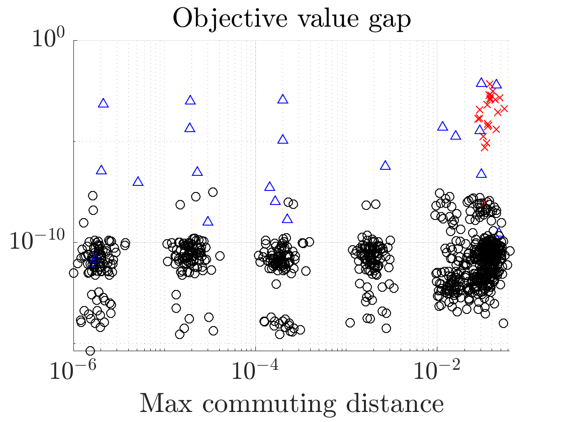
(a)

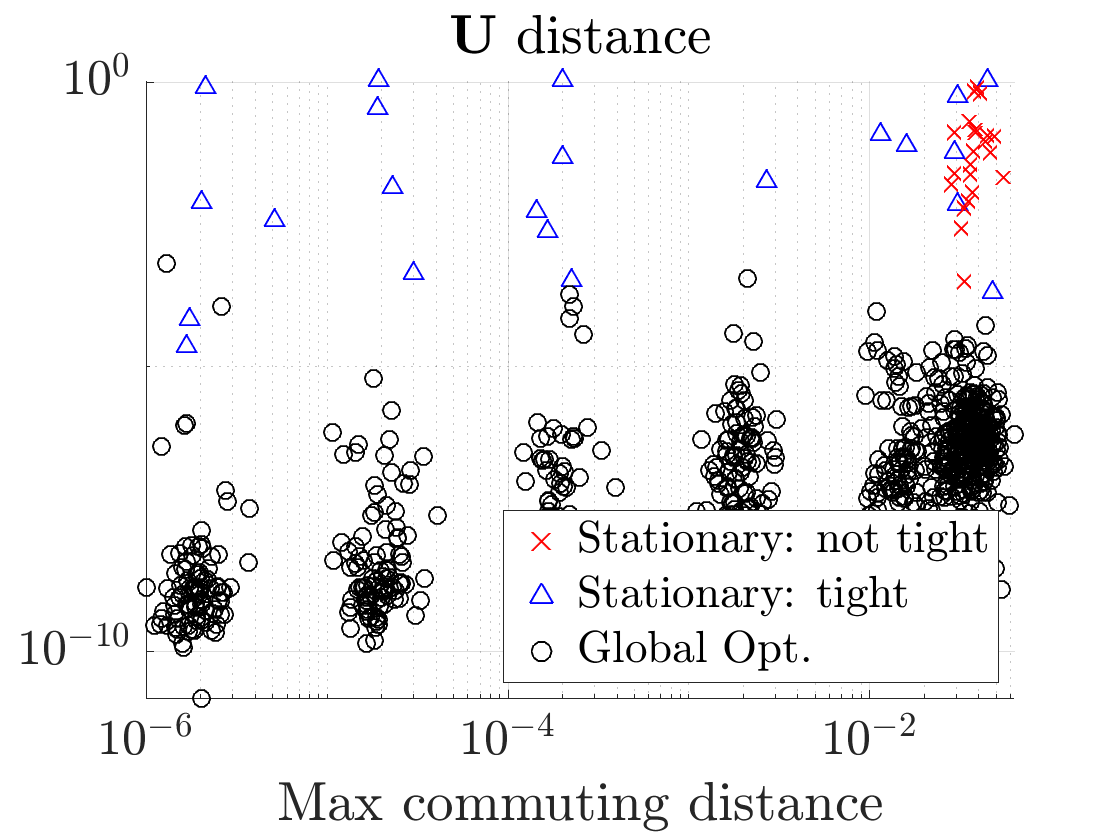
(b)

Figure 1: Numerical simulations for synthetic CJD matrices for $d=10,k=3$ with increasing $\sigma$ and 100 random problem instances for each setting.

HPPCA

We repeat the experiments just described for $\mathbf{M}_{i}$ generated by the model in Eq. 6 for $d=50$, $\bm{\lambda}=[4,3.25,2.5,1.75,1]$, and $L=2$ noise groups with variances $\mathbf{v}=[1,4]$. For each of 100 trials, we draw a random model with a different generative $\mathbf{U}$ for sample sizes $\mathbf{n}=[n_{1},4n_{1}]$, where we sweep through increasing values of $n_{1}$ on the horizontal axis in Fig. 3b. For each experiment, we normalize the $\mathbf{M}_{i}$ by the maximum of their spectral norms, and then record the results obtained from the SDP and StMM solvers with respect to the computed maximum commuting distance of the $\mathbf{M}_{i}$ in Fig. 2. We run StMM for a maximum of 10,000 iterations, and record whether the SDP was tight and the global optimality certification of each StMM run.

Proposition 4.13 suggests that, even with poor SNR like in this example, as the number of data samples increases, the $\mathbf{M}_{i}$ should concentrate to be nearly commuting. This is indeed what we observe: as the number of samples increases in Fig. 3b, the maximum commuting distance of the $\mathbf{M}_{i}$’s decreases, i.e., the simulations move to the left on the horizontal axes of Figs. 2a and 2b. In this nearly-commuting regime, the SDP obtains tight rank-one $\mathbf{X}_{i}$ in 100% of the trials, and interestingly, all of the StMM runs attain the global maximum, suggesting a seemingly benign nonconvex landscape. In contrast, we observed several trials in the low-sample setting where the SDP failed to be tight and a dual certificate was not attained. Also within this regime, several trials of the StMM solver find suboptimal local maxima.

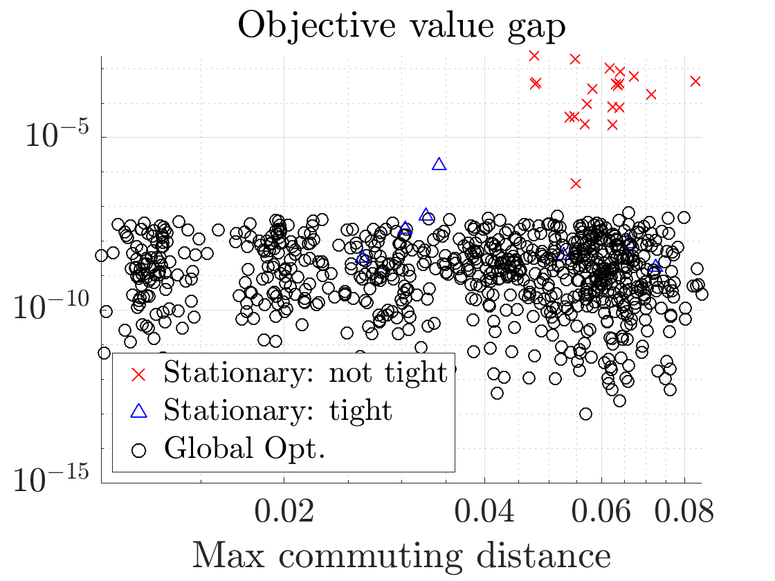
(a)

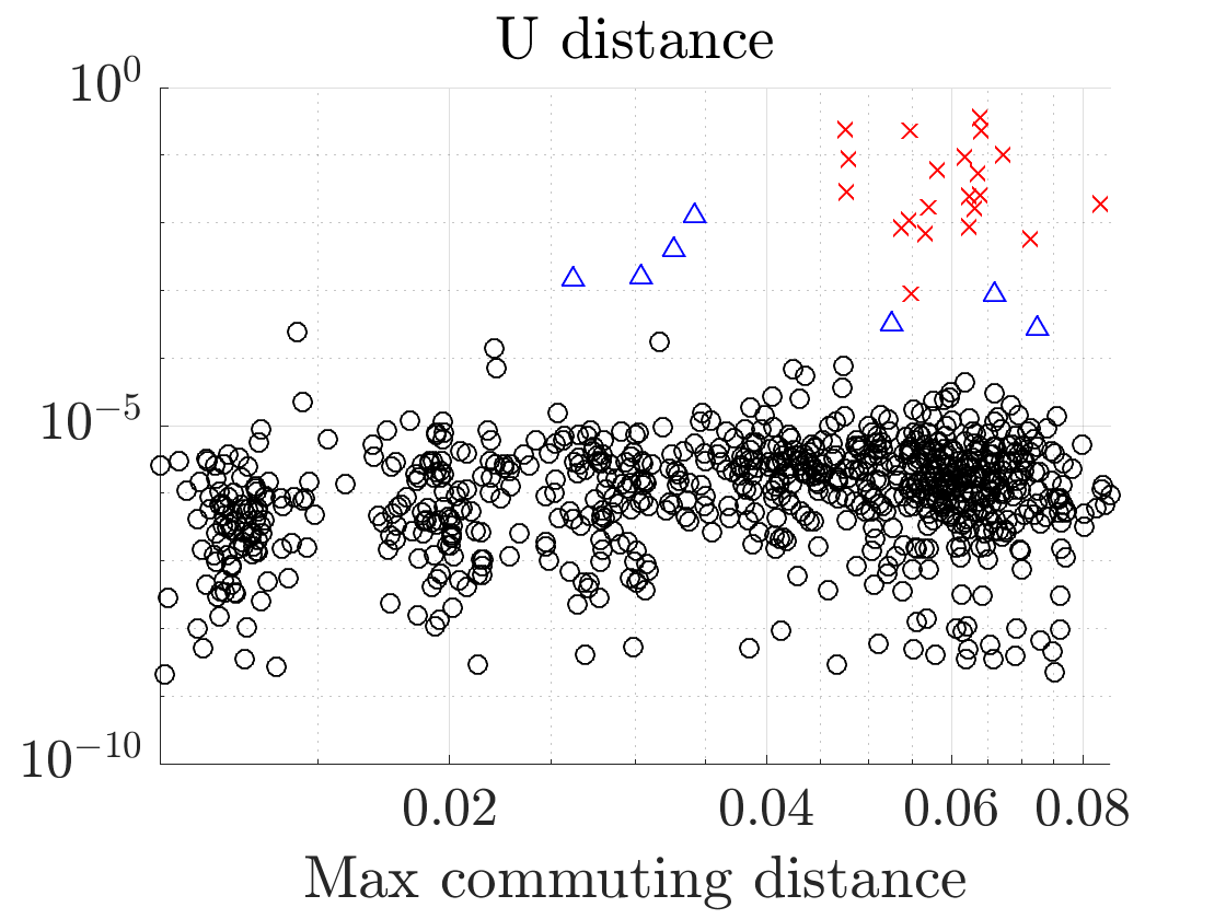
(b)

Figure 2: Numerical simulations for $\mathbf{M}_{i}$ generated by the HPPCA model in Eq. 6 for $d=50$, $k=5$, noise variances $[1,4]$, and $\bm{\lambda}=[4,3.25,2.5,1.75,1]$ with increasing samples $n$. The fractions not shown are tight instances certified as global.

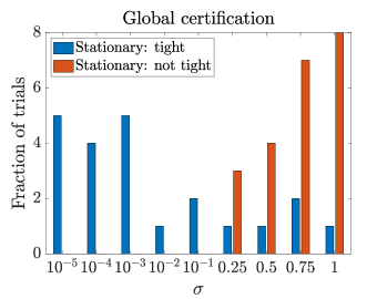
(a) Synthetic CJD matrices for $d=10$, $k=3$ with increasing $\sigma$.

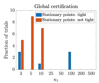
(b) Data matrices generated by the HPPCA model in Eq. 6 with increasing samples $n=(n_{1},4n_{1})$.

Figure 3: Percentages of global certification of StMM solutions out of 100 trials. The fractions not shown are tight instances certified as global.

5.3 Computation time

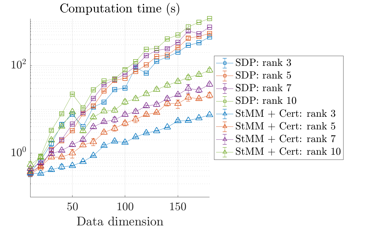
Figure 4: Computation time of Eq. SDP-P versus StMM for 2000 iterations with global certificate check Eq. 5 for HPPCA problems as the data dimension varies. We use $\mathbf{v}=[1,4]$, and $\mathbf{n}=[100,400]$ and make $\bm{\lambda}$ a $k$-length vector with entries equally spaced in the interval $[1,4]$. Markers indicate the median computation time taken over 10 trials, and error bars show the standard deviation.

Fig. 4 compares the scalability of our SDP relaxation in Eq. SDP-P to the StMM solver with the global certificate check in Eq. 5 for synthetically generated HPPCA problems of varying data dimension. We measure the median computation time across 10 independent trials of both algorithms. The experiment strongly demonstrates the computational superiority of the first-order method with our certificate compared to the full SDP. StMM+Certificate scales nearly 60 times better in computation time for the largest dimension with $k=3$ and 15 times for $k=10$, while offering a crucial theoretical guarantee to a nonconvex problem that may contain spurious local maxima. Thus, we can solve the nonconvex problem posed in Eq. 1 using any choice of solver on the Stiefel manifold and perform a fast check of its terminal output for global optimality.

6 Future Work & Conclusion

In this work, we proposed a novel SDP relaxation for the sums of heterogeneous quadratic forms problem, from which we derived a global optimality certificate to check a local solution of a nonconvex program. Our other major contribution proved a continuity result showing sufficient conditions guaranteeing the relaxation has the ROP and providing both theoretical and empirical support that a motivating signal processing application–the HPPCA problem–possesses a tight relaxation in many instances.

While the global certificate scales well compared to solving the full SDP, the LMI feasiblity program still requires forming and factoring $d\times d$ size matrices, requiring storage of $\mathcal{O}(d^{2})$ elements. One exciting possibility is to apply recent works like [51] to our problem, which use randomized algorithms to reduce the storage and arithmetic costs for scalable semidefinite programming. Further, it remains interesting to prove a sufficient analytical certificate, in addition to proving more general sufficient conditions on the $\mathbf{M}_{i}$, to guarantee the ROP.

While we hope the work herein has a positive impact in HPPCA applications like air quality monitoring [29] or medical imaging, we acknowledge the potential for dimensionality reduction algorithms to yield disparate reconstruction errors on populations within a dataset, such as PCA on labeled faces in the wild data set (LFW), which returns higher reconstruction error for women than men even with equal population ratios in the dataset [42]; also see [45].

Appendix A Proofs of Section 2

Proof A.15 (Proof of Lemma 2.4).

The problem is convex and satisfies Slater’s condition, see Lemma A.16. Specifically, at optimality we have $\langle\mathbf{I}-(\sum_{i=1}^{k}\bar{\mathbf{X}}_{i}),\bar{\mathbf{Y}}\rangle=0$ and therefore $\operatorname{tr}(\bar{\mathbf{Y}})=\langle\bar{\mathbf{Y}},\sum_{i=1}^{k}\bar{\mathbf{X}}_{i}\rangle$. Then

$$d^{*} =-\left\langle\sum_{i=1}^{k}\mathbf{M}_{i}+\bar{\mathbf{Z}}_{i}-\bar{\nu}_{i}\mathbf{I},\bar{\mathbf{X}}_{i}\right\rangle-\sum_{i=1}^{k}\bar{\nu}_{i}=-\operatorname{tr}\left(\sum_{i=1}^{k}\mathbf{M}_{i}\bar{\mathbf{X}}_{i}\right),$$

since $\langle\bar{\mathbf{Z}}_{i},\bar{\mathbf{X}}_{i}\rangle=0$ and $\sum_{i=1}^{k}\bar{\nu}_{i}(1-\operatorname{tr}(\bar{\mathbf{X}}_{i}))=0$. Thus, $p^{*}=d^{*}$.

Lemma A.16.

The primal problem in (SDP-P) is strictly feasible for $k<d$.

Proof A.17.

To be strictly feasible we must have $\mathbf{X}_{i}$, $i=1,\dots,k$ such that

$$0\prec\sum_{i=1}^{k}\mathbf{X}_{i}\prec\mathbf{I},\quad\operatorname{tr}(\mathbf{X}_{i})=1,\quad\mathbf{X}_{i}\succ 0,\quad i=1,\dots,k$$

Suppose $\mathbf{X}_{i}=\frac{1}{d}\mathbf{I}$ for all $i$. Then $\operatorname{tr}(\mathbf{X}_{i})=1$ and $\mathbf{X}_{i}\succ 0$ for all $i$, and $\sum_{i=1}^{k}\mathbf{X}_{i}=\frac{k}{d}\mathbf{I}$, satisfying $0\prec\sum_{i=1}^{k}\mathbf{X}_{i}\prec\mathbf{I}$ when $k<d$.

Proof A.18 (Proof of Lemma 2.5).

Since the problem in Eq. SDP-P has a larger constraint set than Eq. 1, any solution to Eq. SDP-P that satisfies the constraints of Eq. 1 is also a solution to this original nonconvex problem.

For the “if” direction, assume that the optimal $\mathbf{X}_{i}$ for Eq. SDP-P have the rank-one property. Since $\operatorname{tr}(\mathbf{X}_{i})=1$ by definition of Eq. SDP-P, when we decompose $\mathbf{X}_{i}=\mathbf{u}_{i}\mathbf{u}_{i}^{\prime}$ we have $\mathbf{u}_{i}$ that are norm-1. In order for $\sum_{i=1}^{k}\mathbf{X}_{i}\preccurlyeq\mathbf{I}$, the $\mathbf{u}_{i}$ must be orthogonal. For the “only if” direction, assume that the solution to the SDP relaxation in (SDP-P) is the optimal solution to the original nonconvex problem in (1) in the sense that $\mathbf{X}_{i}=\mathbf{u}_{i}\mathbf{u}_{i}^{\prime}$ gives the optimal $\mathbf{U}=\left[\begin{matrix}\mathbf{u}_{1}&\cdots&\mathbf{u}_{k}\end{matrix}\right]$. Then by definition we see that the $\mathbf{X}_{i}$ have the rank-one property.

Proof A.19 (Proof of Lemma 2.2).

Without loss of generality, let $\nu_{1}<0$ be the smallest (most negative) coordinate of $\bm{\nu}$, and rewrite the objective in terms of $\mathbf{M}_{1}$ and eliminating $\mathbf{Y}$ as

(8) $$d^{*}=\min_{\nu_{i},\mathbf{Z}_{i}} \operatorname{tr}(\mathbf{Z}_{1}+\mathbf{M}_{1})-d\nu_{1}+\sum_{i=1}^{k}\nu_{i}$$

s.t. $$\mathbf{M}_{i}+\mathbf{Z}_{i}\succcurlyeq\nu_{i}\mathbf{I}\quad\forall i=1,\ldots,k$$

(9) $$\mathbf{M}_{1}+\mathbf{Z}_{1}-\nu_{1}\mathbf{I}=\mathbf{M}_{j}+\mathbf{Z}_{j}-\nu_{j}\mathbf{I}\quad\forall j=2,\ldots,k$$

$$\mathbf{Z}_{i}\succcurlyeq 0\quad\forall i=1,\dots,k.$$

Now consider new variables $\{\tilde{\nu}_{i},\tilde{}\mathbf{Z}_{i}\}_{i=1}^{k}$, where we let $\tilde{\nu}_{1}=0$, $\tilde{\nu}_{i}=\nu_{i}-\nu_{1}$ for $i=2,\dots,k$, and with all the $\mathbf{Z}$ variables unchanged: $\tilde{}\mathbf{Z}_{i}=\mathbf{Z}_{i}$ for all $i$.

These new variables are still feasible. Certainly $\mathbf{M}_{1}+\tilde{}\mathbf{Z}_{1}=\mathbf{M}_{1}+\mathbf{Z}_{1}\succcurlyeq\tilde{\nu}_{1}\mathbf{I}=0$ as both $\mathbf{M}_{1},\mathbf{Z}_{1}$ are PSD. Also $\mathbf{M}_{1}+\tilde{}\mathbf{Z}_{1}-\tilde{\nu}_{1}\mathbf{I}=\mathbf{M}_{j}+\tilde{}\mathbf{Z}_{j}-\tilde{\nu}_{j}\mathbf{I}$, since substituting in, we have $\mathbf{M}_{1}+\mathbf{Z}_{1}=\mathbf{M}_{j}+\mathbf{Z}_{j}-(\nu_{j}-\nu_{1})\mathbf{I}$, which was feasible for the original optimal point. From this last equation note that since $\mathbf{M}_{1}+\mathbf{Z}_{1}\succcurlyeq 0$, then $\mathbf{M}_{j}+\mathbf{Z}_{j}-(\nu_{j}-\nu_{1})\mathbf{I}=\mathbf{M}_{j}+\tilde{}\mathbf{Z}_{j}-\tilde{\nu}_{j}\mathbf{I}\succeq 0$.

However, this yields a contradiction because we have reduced the objective value from

$$\operatorname{tr}(\mathbf{Z}_{1}+\mathbf{M}_{1})-d\nu_{1}+\sum_{i=1}^{k}\nu_{i}\qquad\text{to}\qquad\operatorname{tr}(\mathbf{Z}_{1}+\mathbf{M}_{1})-k\nu_{1}+\sum_{i=1}^{k}\nu_{i}\;.$$

Therefore $\nu_{i}<0$ cannot be optimal.

Lemma A.20.

Suppose $\mathbf{X}_{i}$ for $i=1,\dots,k$ each have trace 1 and satisfy $\lambda_{1}(\mathbf{X}_{i})=1$, and therefore each $\mathbf{X}_{i}$ is rank 1. We decompose $\mathbf{X}_{i}=\mathbf{u}_{i}\mathbf{u}_{i}^{\prime}$ and note that $\mathbf{u}_{i}$ are norm-1. Then $\sum_{i=1}^{k}\mathbf{X}_{i}$ satisfies $0\preccurlyeq\sum_{i=1}^{k}\mathbf{X}_{i}\preccurlyeq\mathbf{I}$ if and only if $\mathbf{u}_{i}^{\prime}\mathbf{u}_{j}=0\quad\forall i\neq j\;.$

Proof A.21.

Forward direction: Suppose $\mathbf{X}=\sum_{i=1}^{k}\mathbf{X}_{i}$ has eigenvalues in $[0,1]$ and $\operatorname{tr}(\mathbf{X})=k$. Since $\text{rank}(\mathbf{X})\leq k$ by subadditivity of rank, this implies both that $\mathbf{X}$ is rank-$k$ and its eigenvalues are either zero or one. Note then that

$$\operatorname{tr}(\mathbf{X}\mathbf{X}^{\prime})=k=\operatorname{tr}\left((\sum_{i}\mathbf{u}_{i}\mathbf{u}_{i}^{\prime})(\sum_{i}\mathbf{u}_{i}\mathbf{u}_{i}^{\prime})\right)=\sum_{i}(\mathbf{u}_{i}^{\prime}\mathbf{u}_{i})^{2}+\operatorname{tr}\left(2\sum_{i\neq j}(\mathbf{u}_{i}^{\prime}\mathbf{u}_{j})^{2}\right)\;.$$

Since $\mathbf{u}_{i}$ are norm-1 then the sum $\sum_{i}(\mathbf{u}_{i}^{\prime}\mathbf{u}_{i})^{2}=k$. This means

$$\operatorname{tr}\left(2\sum_{i\neq j}(\mathbf{u}_{i}^{\prime}\mathbf{u}_{j})^{2}\right)=0\;,$$

which is true if and only if $\mathbf{u}_{i}^{\prime}\mathbf{u}_{j}=0$.

The backward direction is immediate because when $\mathbf{u}_{i}^{\prime}\mathbf{u}_{j}=0$ for $i\neq j$, $\sum_{i=1}^{k}\mathbf{u}_{i}\mathbf{u}_{i}^{\prime}$ is the singular value decomposition of $\mathbf{X}$ with $k$ eigenvalues equal to one.

Proof A.22 (Proof of Lemma 2.3).

Suppose $\mathbf{Z}_{i}$ is rank $d-1$. By complementarity at optimality, we have $\mathbf{Z}_{i}\mathbf{X}_{i}=0\quad\forall i$, which means $\mathbf{X}_{i}$ lies in the nullspace of $\mathbf{Z}_{i}$, which has dimension 1, so each $\mathbf{X}_{i}$ is rank-1. By primal feasibility, $\operatorname{tr}(\mathbf{X}_{i})=1$, so $\lambda_{1}(\mathbf{X}_{i})=1\quad\forall i=1,\ldots,k$. By Lemma A.20, the optimal solution is an orthogonal projection matrix, and the optimal $\mathbf{X}_{i}$ are orthogonal.

Appendix B Proof of Theorem 4.6

Lemma B.23.

Let $\mathcal{F}(\mathbf{U})$ denote the objective function with respect to $\mathbf{U}$ in Eq. 1 over $\text{St}(k,d)$. If a point $\mathbf{U}\in\text{St}(k,d)$ is a second-order stationary point (SOSP) of $\mathcal{F}$, then

$$\bm{\Lambda} =\mathbf{U}^{\prime}\sum_{i=1}^{k}\mathbf{M}_{i}\mathbf{U}\mathbf{E}_{i}~{}~{}\text{is symmetric},~{}\text{and}$$

$$-\sum_{i=1}^{k}\langle\dot{\mathbf{U}},\mathbf{M}_{i}\dot{\mathbf{U}}\mathbf{E}_{i}\rangle +\langle\dot{\mathbf{U}}\bm{\Lambda},\dot{\mathbf{U}}\rangle\geq 0\quad\forall\dot{\mathbf{U}}\in\mathbb{R}^{d\times k}~{}\text{such that}~{}\dot{\mathbf{U}}^{\prime}\mathbf{U}+\mathbf{U}^{\prime}\dot{\mathbf{U}}=0.$$

Proof B.24.

Taking $\bar{}\mathcal{F}$ to be the quadratic function in Eq. 1 (scaled by $\frac{1}{2}$) over Euclidean space, the Euclidean gradient $\bm{\nabla}\bar{}\mathcal{F}(\mathbf{U})=\sum_{i=1}^{k}\mathbf{M}_{i}\mathbf{U}\mathbf{E}_{i}=\begin{bmatrix}\mathbf{M}_{1}\mathbf{u}_{1}&\cdots&\mathbf{M}_{k}\mathbf{u}_{k}\end{bmatrix}$, where $\mathbf{E}_{i}:=\mathbf{e}_{i}\mathbf{e}_{i}^{\prime}\in\mathbb{R}^{k\times k}$ and $\mathbf{e}_{i}$ is the $i^{th}$ standard basis vector in $\mathbb{R}^{k}$. The Euclidean Hessian can also easily be derived as $\bm{\nabla}^{2}\bar{}\mathcal{F}(\mathbf{U})[\dot{\mathbf{U}}]=\sum_{i=1}^{k}\mathbf{M}_{i}\dot{\mathbf{U}}\mathbf{E}_{i}$. Restricting $\bar{}\mathcal{F}$ to the Stiefel manifold, let $\mathcal{F}:=\bar{}\mathcal{F}|_{\text{St}(k,d)}$. If $\mathbf{U}\in\text{St}(k,d)$ is a SOSP of Eq. 1, then

(10) $$\bm{\nabla}\mathcal{F}(\mathbf{U})=0\quad\text{and}\quad\bm{\nabla}^{2}\mathcal{F}(\mathbf{U})\preceq 0,$$

where $\bm{\nabla}\mathcal{F}$ and $\bm{\nabla}^{2}\mathcal{F}$ denote the Riemannian gradient and Hessian of $\mathcal{F}$, respectively.

From [2], the gradient on the manifold for SOSPs $\mathbf{U}$ satisfies

(11) $$\bm{\nabla}\mathcal{F}=\bm{\nabla}\bar{}\mathcal{F}-\mathbf{U}\text{sym}(\mathbf{U}^{\prime}\bm{\nabla}\bar{}\mathcal{F}(\mathbf{U})) =(\mathbf{I}-\mathbf{U}\mathbf{U}^{\prime})\bm{\nabla}\bar{}\mathcal{F}+\mathbf{U}\text{skew}(\mathbf{U}^{\prime}\bm{\nabla}\bar{}\mathcal{F}),$$

(12) $$=(\mathbf{I}-\mathbf{U}\mathbf{U}^{\prime})\sum_{i=1}^{k}\mathbf{M}_{i}\mathbf{U}\mathbf{E}_{i}+{\frac{1}{2}}\mathbf{U}\sum_{i=1}^{k}[\mathbf{U}^{\prime}\mathbf{M}_{i}\mathbf{U},\mathbf{E}_{i}]$$

(13) $$=0,$$

where $\text{sym}(\mathbf{A})=\frac{1}{2}(\mathbf{A}+\mathbf{A}^{\prime})$, $\text{skew}(\mathbf{A})=\frac{1}{2}(\mathbf{A}-\mathbf{A}^{\prime})$, and $[\mathbf{A},\mathbf{B}]=\mathbf{A}\mathbf{B}-\mathbf{B}\mathbf{A}$. We note the left and right expressions of the Riemannian gradient in Eq. 12 lie in the orthogonal complement of $\text{Span}(\mathbf{U})$ and the $\text{Span}(\mathbf{U})$, respectively, so $\bm{\nabla}\mathcal{F}$ vanishes if and only if $(\mathbf{I}-\mathbf{U}\mathbf{U}^{\prime})\bm{\nabla}\bar{}\mathcal{F}=0$, and $\sum_{i=1}^{k}[\mathbf{U}^{\prime}\mathbf{M}_{i}\mathbf{U},\mathbf{E}_{i}]=0$, implying $\mathbf{U}^{\prime}\bm{\nabla}\bar{}\mathcal{F}=\bm{\nabla}\bar{}\mathcal{F}^{\prime}\mathbf{U}$. Letting $\bm{\Lambda}:=\text{sym}(\mathbf{U}^{\prime}\bm{\nabla}\bar{}\mathcal{F})$, this also implies

(14) $$\mathbf{U}\bm{\Lambda}=\bm{\nabla}\bar{}\mathcal{F}=\sum_{i=1}^{k}\mathbf{M}_{i}\mathbf{U}\mathbf{E}_{i},$$

and multiplying both sides by $\mathbf{U}^{\prime}$ yields the expression for $\bm{\Lambda}$, which is symmetric as shown above so we can drop the $\text{sym}(\cdot)$ operator.

It can be shown the Riemannian Hessian is negative semidefinite if and only if

(15) $$\langle\dot{\mathbf{U}},\bm{\nabla}^{2}\bar{}\mathcal{F}(\mathbf{U})[\dot{\mathbf{U}}]-\dot{\mathbf{U}}\bm{\Lambda}\rangle\leq 0$$

for all $\dot{\mathbf{U}}\in T_{\mathbf{U}}\text{St}(d,k)$, where $T_{\mathbf{U}}\text{St}(d,k)$ is the tangent space of the Stiefel manifold, i.e. the set $T_{\mathbf{U}}\text{St}(d,k)=\{\dot{\mathbf{U}}\in\mathbb{R}^{d\times k}:\mathbf{U}^{\prime}\dot{\mathbf{U}}+\dot{\mathbf{U}}^{\prime}\mathbf{U}=0\}$. Plugging in the expressions for $\bm{\Lambda}$ and the Hessian of $\bar{}\mathcal{F}$ yield the main result.

The following lemma is adapted from [8, Corollary 4.2]

Lemma B.25.

Let $\bar{\mathbf{U}}\in\mathbb{R}^{d\times k}$ be a second-order stationary point of Eq. 1 and $\mathbf{M}_{i}\succeq 0$ for all $i\in[k]$. Then $\bar{\bm{\Lambda}}=\bar{\mathbf{U}}^{\prime}\sum_{i=1}^{k}\mathbf{M}_{i}\bar{\mathbf{U}}\mathbf{E}_{i}$ is positive semidefinite.

Proof B.26.

Since $k<d$, there exists a unit vector $\mathbf{z}$ in the span of $\bar{\mathbf{U}}_{\perp}\in\mathbb{R}^{d\times d-k}$ where $\bar{\mathbf{U}}^{\prime}\bar{\mathbf{U}}_{\perp}=0$. Let $\mathbf{a}=[a_{1},\ldots,a_{k}]^{\prime}\in\mathbb{R}^{k}$ be an arbitrary nonzero vector. Let $\dot{\mathbf{U}}:=\mathbf{z}\mathbf{a}^{\prime}$, and let $\bar{\bm{\Lambda}}=\sum_{i=1}^{k}\bar{\mathbf{U}}^{\prime}\mathbf{M}_{i}\bar{\mathbf{U}}\mathbf{E}_{i}$. Then clearly $\bar{\mathbf{U}}^{\prime}\dot{\mathbf{U}}=0$, and $\bar{\mathbf{U}}^{\prime}\dot{\mathbf{U}}+\dot{\mathbf{U}}^{\prime}\bar{\mathbf{U}}=0$, so the second-order stationary necessary condition in Lemma B.23 applies:

(16) $$\mathbf{a}^{\prime}\bar{\bm{\Lambda}}\mathbf{a}=\langle\dot{\mathbf{U}}\bar{\bm{\Lambda}},\dot{\mathbf{U}}\rangle\geq\sum_{i=1}^{k}\langle\dot{\mathbf{U}},\mathbf{M}_{i}\dot{\mathbf{U}}\mathbf{E}_{i}\rangle=\sum_{i=1}^{k}(a_{i})^{2}\mathbf{z}^{\prime}\mathbf{M}_{i}\mathbf{z}\geq 0.$$

Therefore, since $\mathbf{a}^{\prime}\bar{\bm{\Lambda}}\mathbf{a}\geq 0$ for arbitrary $\mathbf{a}$, $\bar{\bm{\Lambda}}$ is positive semidefinite.

Proof B.27 (Proof of Theorem 4.6).

By Lemma 2.4, primal and dual feasible solutions of Eq. SDP-P and Eq. SDP-D, $\bar{\mathbf{X}}_{i},\bar{\mathbf{Z}}_{i},\bar{\mathbf{Y}},\bar{\bm{\nu}}$, are simultaneously optimal if and only if they satisfy the following Karush-Kuhn Tucker (KKT) conditions [13], where the variables and constraints are indexed by $i\in[k]$:

(KKT-a) $$\bar{\mathbf{X}}_{i}\succeq 0,\quad\sum_{i=1}^{k}\bar{\mathbf{X}}_{i}\preceq\mathbf{I},\quad\operatorname{tr}(\bar{\mathbf{X}}_{i})=1$$

(KKT-b) $$\bar{\mathbf{Y}}=\mathbf{M}_{i}+\bar{\mathbf{Z}}_{i}-\bar{\nu}_{i}\mathbf{I},\qquad\bar{\mathbf{Y}}\succeq 0$$

(KKT-c) $$\langle\mathbf{I}-\sum_{i=1}^{k}\bar{\mathbf{X}}_{i},\bar{\mathbf{Y}}\rangle=0$$

(KKT-d) $$\langle\bar{\mathbf{Z}}_{i},\bar{\mathbf{X}}_{i}\rangle=0$$

(KKT-e) $$\bar{\mathbf{Z}}_{i}\succeq 0.$$

Similar to the work in [50], our strategy is then to construct $\bar{\mathbf{X}}_{i}$ and $\bar{\mathbf{Y}},\bar{\mathbf{Z}}_{i},\bar{\bm{\nu}}$ satisfying these conditions. Given $\bar{\mathbf{U}}$ and $\bar{\bm{\nu}}$ in the statement of the theorem, we define $\bar{\mathbf{X}}_{i}=\bar{\mathbf{u}}_{i}\bar{\mathbf{u}}_{i}^{\prime}$, $\bar{\mathbf{Y}}=\bar{\mathbf{U}}(\bar{\bm{\Lambda}}-\mathbf{D}_{\bar{\bm{\nu}}})\bar{\mathbf{U}}^{\prime}$, and $\bar{\mathbf{Z}}_{i}=\bar{\mathbf{Y}}+\bar{\nu}_{i}\mathbf{I}-\mathbf{M}_{i}$. By construction, $\bar{\mathbf{X}}_{i}$ satisfy Eq. KKT-a, and it is clear that $\bar{\mathbf{Y}}=\mathbf{M}_{i}+\bar{\mathbf{Z}}_{i}-\bar{\bm{\nu}}_{i}\mathbf{I}$ satisfies Eq. KKT-b. One can also verify that $\langle\mathbf{I}-\bar{\mathbf{X}},\bar{\mathbf{Y}}\rangle=0$ by construction, thus satisfying Eq. KKT-c. So it remains to show $\bar{\mathbf{Y}}\succeq 0$, $\langle\bar{\mathbf{Z}}_{i},\bar{\mathbf{X}}_{i}\rangle=0$, and $\bar{\mathbf{Z}}_{i}\succeq 0$.

The assumption that $\bar{\bm{\Lambda}}\succeq\mathbf{D}_{\bar{\bm{\nu}}}$ ensures $\bar{\mathbf{Y}}\succeq 0$ (KKT-b). We note that we have shown in Lemma B.23 and Lemma B.25 that $\bar{\bm{\Lambda}}$ is symmetric PSD, which is a necessary condition for this assumption to hold, given the fact that the Lagrange multipliers $\bar{\nu}_{i}$ corresponding to the trace constraints are nonnegative by Lemma 2.2.

Moreover, $\bar{\mathbf{Z}}_{i}\succeq 0$ by the assumption in Eq. 5, satisfying Eq. KKT-e. We finally verify Eq. KKT-d, i.e. $\langle\bar{\mathbf{Z}}_{i},\bar{\mathbf{X}}_{i}\rangle=0$, with $\bar{\mathbf{U}}=[\bar{\mathbf{u}}_{1}\cdots\bar{\mathbf{u}}_{k}]$:

$$\langle\bar{\mathbf{Z}}_{i},\bar{\mathbf{X}}_{i}\rangle =\langle\bar{\mathbf{Y}}+\bar{\nu}_{i}\mathbf{I}-\mathbf{M}_{i},\bar{\mathbf{X}}_{i}\rangle=\langle\bar{\mathbf{U}}(\bar{\bm{\Lambda}}-\mathbf{D}_{\bar{\bm{\nu}}})\bar{\mathbf{U}}^{\prime}+\bar{\nu}_{i}\mathbf{I}-\mathbf{M}_{i},\bar{\mathbf{u}}_{i}\bar{\mathbf{u}}_{i}^{\prime}\rangle$$

$$=\bar{\mathbf{u}}_{i}^{\prime}\bar{\mathbf{U}}\bar{\mathbf{U}}^{\prime}\sum_{j=1}^{k}\mathbf{M}_{j}\bar{\mathbf{U}}\mathbf{E}_{j}\bar{\mathbf{U}}^{\prime}\bar{\mathbf{u}}_{i}-\bar{\mathbf{u}}_{i}^{\prime}\bar{\mathbf{U}}\mathbf{D}_{\bar{\bm{\nu}}}\bar{\mathbf{U}}^{\prime}\bar{\mathbf{u}}_{i}+\bar{\nu}_{i}-\bar{\mathbf{u}}_{i}^{\prime}\mathbf{M}_{i}\bar{\mathbf{u}}_{i}$$

$$=\mathbf{e}_{i}^{\prime}\bar{\mathbf{U}}^{\prime}\sum_{j=1}^{k}\mathbf{M}_{j}\bar{\mathbf{u}}_{j}\mathbf{e}_{j}^{\prime}\mathbf{e}_{i}-\mathbf{e}_{i}^{\prime}\mathbf{D}_{\bar{\bm{\nu}}}\mathbf{e}_{i}+\bar{\nu}_{i}-\bar{\mathbf{u}}_{i}^{\prime}\mathbf{M}_{i}\bar{\mathbf{u}}_{i}$$

$$=\bar{\mathbf{u}}_{i}^{\prime}\mathbf{M}_{i}\bar{\mathbf{u}}_{i}-\bar{\nu}_{i}+\bar{\nu}_{i}-\bar{\mathbf{u}}_{i}^{\prime}\mathbf{M}_{i}\bar{\mathbf{u}}_{i}=0.$$

See Appendix E for additional remarks.

Appendix C Proof of Theorem 4.10

We start this section by giving general convex analysis results that allow us to prove Theorem 4.10.

Let ${\cal C}\subseteq\mathbb{R}^{n}$ be a closed, convex set. For all $\mathbf{c}\in{\cal C}$, consider a primal-dual pair of linear conic programs parameterized by $c$:

(17) $$p(\mathbf{c}) :=\min_{\mathbf{x}}\{\mathbf{c}^{T}\mathbf{x}:\mathbf{A}\mathbf{x}=\mathbf{b},\mathbf{x}\in{\cal K}\}$$

(18) $$d(\mathbf{c}) :=\max_{\mathbf{y}}\{\mathbf{b}^{T}\mathbf{y}:\mathbf{c}-\mathbf{A}^{T}\mathbf{y}\in{\cal K}^{*}\}$$

Here, the data $\mathbf{A}\in\mathbb{R}^{m\times n}$ and $\mathbf{b}\in\mathbb{R}^{m}$ are fixed; ${\cal K}\subseteq\mathbb{R}^{n}$ is a closed, convex cone; and ${\cal K}^{*}:=\{\mathbf{s}\in\mathbb{R}^{n}:\mathbf{s}^{T}\mathbf{x}\geq 0\ \forall\ \mathbf{x}\in{\cal K}\}$ is its polar dual. We imagine, in particular, that ${\cal K}$ is a direct product of a nonnegative orthant, second-order cones, and positive semidefinite cones, corresponding to linear, second-order-cone, and semidefinite programming.

Define $\text{Feas}(P):=\{\mathbf{x}\in{\cal K}:\mathbf{A}\mathbf{x}=\mathbf{b}\}$ and $\text{Feas}(D;\mathbf{c}):=\{\mathbf{y}:\mathbf{c}-\mathbf{A}^{T}\mathbf{y}\in{\cal K}^{*}\}$ to be the feasible sets of $(P;\mathbf{c})$ and $(D;\mathbf{c})$, respectively. We assume:

Assumption C.27.1.

$\text{Feas}(P)$ is interior feasible, and $\text{Feas}(D;\mathbf{c})$ is interior feasible for all $\mathbf{c}\in{\cal C}$.

Then, for all $\mathbf{c}$, strong duality holds between $(P;\mathbf{c})$ and $(D;\mathbf{c})$ in the sense that $p(\mathbf{c})=d(\mathbf{c})$ and both $p(\mathbf{c})$ and $d(\mathbf{c})$ are attained in their respective problems. Accordingly, we also define

$$\text{Opt}(D;\mathbf{c}):=\{\mathbf{y}\in\text{Feas}(D;\mathbf{c}):\mathbf{b}^{T}\mathbf{y}=d(\mathbf{c})\}$$

to be the nonempty, dual optimal solution set for each $\mathbf{c}\in{\cal C}$.

In addition, we assume the existence of linear constraints $\mathbf{f}-\mathbf{E}^{T}\mathbf{y}\geq 0$, independent of $\mathbf{c}$, such that

$$\text{Extra}(D):=\{\mathbf{y}:\mathbf{f}-\mathbf{E}^{T}\mathbf{y}\geq 0\}$$

satisfies:

Assumption C.27.2.

For all $\mathbf{c}\in{\cal C}$, $\text{Feas}(D;\mathbf{c})\cap\text{Extra}(D)$ is interior feasible and bounded, and $\text{Opt}(D;\mathbf{c})\subseteq\text{Extra}(D)$.

In words, irrespective of $\mathbf{c}$, the extra constraints $\mathbf{f}-\mathbf{E}^{T}\mathbf{y}\geq 0$ bound the dual feasible set without cutting off any optimal solutions and while still maintaining interior, including interiority with respect to $\mathbf{f}-\mathbf{E}^{T}\mathbf{y}\geq 0$. Note also that Assumption C.27.2 implies the recession cone of $\text{Feas}(D;\mathbf{c})\cap\text{Extra}(D)$ is trivial for (and independent of) all $\mathbf{c}$, i.e., $\{\bm{\Delta}\mathbf{y}:-\mathbf{A}^{T}\bm{\Delta}\mathbf{y}\in{\cal K}^{*},-\mathbf{E}^{T}\bm{\Delta}\mathbf{y}\geq 0\}=\{0\}$.

We first prove a continuity result related to the dual feasible set, in which we use the following definition of a convergent sequence of bounded sets in Euclidean space: a sequence of bounded sets $\{L^{k}\}$ converges to a bounded set $\bar{L}$, written $\{L^{k}\}\to\bar{L}$, if and only if: (i) given any sequence $\{\mathbf{y}^{k}\in L^{k}\}$, every limit point $\bar{}\mathbf{y}$ of the sequence satisfies $\bar{}\mathbf{y}\in\bar{L}$; and (ii) every member $\bar{}\mathbf{y}\in\bar{L}$ is the limit point of some sequence $\{\mathbf{y}^{k}\in L^{k}\}$.

Lemma C.28.

Under Assumptions C.27.1 and C.27.2, let $\{\mathbf{c}^{k}\in{\cal C}\}\to\bar{}\mathbf{c}$ be any convergent sequence. Then

$$\left\{\text{Feas}(D;\mathbf{c}^{k})\cap\text{Extra}(D)\right\}\ \ \to\ \ \text{Feas}(D;\bar{}\mathbf{c})\cap\text{Extra}(D).$$

Proof C.29.

See Appendix G in the supplement for the proof.

Lemma C.30.

Under Assumptions C.27.1 and C.27.2, let $\{\mathbf{c}^{k}\in{\cal C}\}\to\bar{}\mathbf{c}$ be any convergent sequence. Assume

$$\left\{\text{Opt}(D;\mathbf{c}^{k})\right\}\ \ \to\ \ \text{Opt}(D;\bar{}\mathbf{c}).$$

Proof C.31.

See Appendix H in the supplement for the proof.

Finally, for given $\mathbf{c}\in{\cal C}$ and fixed $\mathbf{y}^{0}\in\mathbb{R}^{m}$, we define the function

$$y(\mathbf{c}):=y(\mathbf{c};\mathbf{y}^{0})=\text{argmin}\{\|\mathbf{y}-\mathbf{y}^{0}\|:\mathbf{y}\in\text{Opt}(D;\mathbf{c})\},$$

i.e., $y(\mathbf{c})$ equals the point in $\text{Opt}(D;\mathbf{c})$, which is closest to $\mathbf{y}^{0}$. Since $\text{Opt}(D;\mathbf{c})$ is closed and convex, $y(\mathbf{c})$ is well defined. We next use Lemma C.30 to show that $y(\mathbf{c})$ is continuous in $\mathbf{c}$.

Proposition C.32.

Under the Assumptions C.27.1 and C.27.2, given $\mathbf{y}^{0}\in\mathbb{R}^{m}$, the function $y(\mathbf{c}):=y(\mathbf{c};\mathbf{y}^{0})$ is continuous in $\mathbf{c}$.

Proof C.33.

We must show that, for any convergent $\{\mathbf{c}^{k}\}\to\bar{}\mathbf{c}$, we also have convergence $\{y(\mathbf{c}^{k})\}\to y(\bar{}\mathbf{c})$. This follows because $\{\text{Opt}(D;\mathbf{c}^{k})\}\to\text{Opt}(D;\bar{}\mathbf{c})$ by Lemma C.30.

Theorem 4.10 uses Proposition C.32 in its proof. Here we discuss how the primal-dual pair (SDP-P)-(SDP-D) satisfy the assumptions for the proposition. We would like to establish conditions under which (SDP-P) has the rank-1 property. For this, we apply the general theory developed above, specifically Proposition C.32. To show that the general theory applies, we must define the closed, convex set ${\cal C}$, which contains the set of admissible objective matrices/coefficients $(\mathbf{M}_{1},\ldots,\mathbf{M}_{k})$ and which satisfies Assumptions C.27.1 and C.27.2. In particular, for a fixed, user-specified upper bound $\mu>0$, we define ${\cal C}:=\{\mathbf{c}=(\mathbf{M}_{1},\ldots,\mathbf{M}_{k}):0\preceq\mathbf{M}_{i}\preceq\mu\mathbf{I}\quad\forall\ i=1,\ldots,k\}$ to be our set of admissible coefficient $k$-tuples.

We know that both (SDP-P) and (SDP-D) have interior points for all $\mathbf{c}\in{\cal C}$, so that strong duality holds. For the dual in particular, the equation $\mu\mathbf{I}=\mathbf{M}_{i}+((\mu+\epsilon)\mathbf{I}-\mathbf{M}_{i})-\epsilon\mathbf{I}$ shows that, for all $\epsilon>0$, $\mathbf{Y}(\epsilon):=\mu\mathbf{I},~{}~{}\mathbf{Z}(\epsilon)_{i}:=(\mu+\epsilon)\mathbf{I}-\mathbf{M}_{i},~{}~{}\nu(\epsilon)_{i}:=\epsilon$ is interior feasible with objective value $d\mu+k\epsilon$. In particular, the redundant constraint $\bm{\nu}\geq 0$ is satisfied strictly. This verifies Assumption C.27.1.

We next verify Assumption C.27.2. Since the objective value just mentioned is independent of $\mathbf{c}=(\mathbf{M}_{1},\ldots,\mathbf{M}_{k})$, we can take $\epsilon=1$ and enforce the extra constraint $\operatorname{tr}(\mathbf{Y})+\sum_{i=1}^{k}\nu_{i}\leq d\mu+k$ without cutting off any dual optimal solutions and while still maintaining interior. In particular, the solution $(\mathbf{Y}(\tfrac{1}{2}),\mathbf{Z}(\tfrac{1}{2})_{i},\bm{\nu}(\tfrac{1}{2})_{i})$ corresponding to $\epsilon=\tfrac{1}{2}$ satisfies the new, extra constraint strictly. Finally, note that $\operatorname{tr}(\mathbf{Y})+\sum_{i}\nu_{i}\leq d\mu+k$ bounds $\mathbf{Y}$ and $\bm{\nu}$ in the presence of the constraints $\mathbf{Y}\succeq 0$ and $\bm{\nu}\geq 0$, and consequently the constraint $\mathbf{Z}_{i}=\mathbf{Y}-\mathbf{M}_{i}+\nu_{i}\mathbf{I}$ bounds $\mathbf{Z}_{i}$ for each $i$.

We now repeat the discussion leading up to Theorem 4.10 for completeness. The first lemma says that the diagonal problem has dual variables $\mathbf{Z}_{i}$ such that ${\text{rank}}(\mathbf{Z}_{i})\geq d-1$, implying that the primal variables $\mathbf{X}_{i}$ are rank-1.

Proof C.34 (Proof of Lemma 4.8).

Because of the jointly diagonalizable property, we may assume without loss of generality that each $\mathbf{M}_{i}$ is diagonal. So (SDP-P) is equivalent to the assignment LP

$$\max\left\{\sum_{i=1}^{k}\operatorname{diag}(\mathbf{M}_{i})^{\prime}\operatorname{diag}(\mathbf{X}_{i}):\begin{array}[]{l}\mathbf{e}^{\prime}\operatorname{diag}(\mathbf{X}_{i})=1,\ \operatorname{diag}(\mathbf{X}_{i})\geq 0\ \ \forall\ i=1,\ldots,k\\ \sum_{i=1}^{k}\operatorname{diag}(\mathbf{X}_{i})\leq\mathbf{e}\end{array}\right\},$$

where $\mathbf{e}$ is the vector of all ones, and (SDP-D) is equivalent to the LP

$$\min\left\{\mathbf{e}^{\prime}\operatorname{diag}(\mathbf{Y})+\sum_{i=1}^{k}\nu_{i}:\begin{array}[]{l}\operatorname{diag}(\mathbf{Y})=\operatorname{diag}(\mathbf{M}_{i})+\operatorname{diag}(\mathbf{Z}_{i})-\nu_{i}\mathbf{e}\ \ \forall\ i=1,\ldots,k\\ \operatorname{diag}(\mathbf{Z}_{i})\geq 0\ \ \forall\ i=1,\ldots,k,\quad\operatorname{diag}(\mathbf{Y})\geq 0\\ \end{array}\right\}.$$

Since the primal is an assignment problem, its unique optimal solution has the property that each $\operatorname{diag}(\mathbf{X}_{i})$ is a standard basis vector (i.e., each has a single entry equal to 1 and all other entries equal to 0). By the Goldman-Tucker strict complementarity theorem for LP, there exists an optimal primal-dual pair such that $\operatorname{diag}(\mathbf{X}_{i})+\operatorname{diag}(\mathbf{Z}_{i})>0$ for each $i$. Hence, there exists a dual optimal solution with ${\text{rank}}(\mathbf{Z}_{i})\geq d-1$ for each $i$, as desired.

Proof C.35 (Proof of Theorem 4.10).

Using Lemma 4.8, let $\mathbf{y}^{0}:=(\bar{}\mathbf{Y},\bar{}\mathbf{Z}_{i},\bar{\nu}_{i})$ be the optimal solution of the dual problem (SDP-D) for $\bar{}\mathbf{c}=(\bar{}\mathbf{M}_{1},\ldots,\bar{}\mathbf{M}_{k})$, which has ${\text{rank}}(\bar{}\mathbf{Z}_{i})\geq d-1$ for all $i$. Then by Proposition C.32, the function $y(\mathbf{c}):=y(\mathbf{c};\mathbf{y}^{0})$, which returns the optimal solution of (SDP-D) for $\mathbf{c}=(\mathbf{M}_{1},\ldots,\mathbf{M}_{k})$ closest to $\mathbf{y}^{0}$, is continuous in $\mathbf{c}$. It follows that the preimage

$$y^{-1}\left(\{(\mathbf{Y},\mathbf{Z}_{i},\nu_{i}):{\text{rank}}(\mathbf{Z}_{i})\geq d-1\ \ \forall\ i\}\right)$$

contains $\bar{}\mathbf{c}$ and is an open set because the set of all $(\mathbf{Y},\mathbf{Z}_{i},\nu_{i})$ with ${\text{rank}}(\mathbf{Z}_{i})\geq d-1$ is an open set. After intersecting with ${\cal C}$, this full-dimensional set $\bar{\cal C}$ proves the theorem via the complementarity of the KKT conditions of the assignment LP, ${\text{rank}}(\mathbf{Z}_{i})=d-1$ for $i=1,\ldots,k$, and Lemma 2.3.

The next corollary is a slightly more general version of Corollary 4.12, which shows that for a general tuple of almost commuting matrices $\mathbf{c}:=(\mathbf{M}_{1},\ldots,\mathbf{M}_{k})$ that are CJD, Eq. SDP-P is tight and has the rank-1 property. The result draws upon Lin’s Theorem, given in Lemma I.61 of the supplement.

Proof C.36 (Proof of Corollary 4.12).

The general result follows from directly applying Lemma I.61 to each $\mathbf{M}_{i}$, and for the instance of problem Eq. 2, we apply Lemma I.61 to each $\mathbf{A}_{\ell}$. Then there exist Hermitian symmetric matrices $\bar{}\mathbf{A}_{\ell}$ such that $\|[\bar{}\mathbf{A}_{\ell},\bar{}\mathbf{A}_{m}]\|=0$ for all $\ell,m\in[L]$ such that $\|\mathbf{A}_{\ell}-\bar{}\mathbf{A}_{\ell}\|\leq\epsilon(\delta)$ for all $\ell\in[L]$. Let $\bar{}\mathbf{M}_{i}:=\sum_{\ell=1}^{L}w_{\ell,i}\bar{}\mathbf{A}_{\ell}$. Then the matrices $\bar{}\mathbf{M}_{i}$ commute and are jointly diagonalizable:

(19) $$[\bar{}\mathbf{M}_{i},\bar{}\mathbf{M}_{j}]=\bar{}\mathbf{M}_{i}\bar{}\mathbf{M}_{j}-\bar{}\mathbf{M}_{j}\bar{}\mathbf{M}_{i} =2\sum_{\ell\neq m}^{L}w_{\ell,i}w_{m,j}(\bar{}\mathbf{A}_{\ell}\bar{}\mathbf{A}_{m}-\bar{}\mathbf{A}_{m}\bar{}\mathbf{A}_{\ell})=0.$$

Now we measure the distance between each $\mathbf{M}_{i}$ and $\bar{\mathbf{M}}_{i}$:

(20) $$\|\mathbf{M}_{i}-\bar{}\mathbf{M}_{i}\|=\|\sum_{\ell=1}^{L}w_{\ell,i}(\mathbf{A}_{\ell}-\bar{}\mathbf{A}_{\ell})\|\leq\sum_{\ell=1}^{L}w_{\ell,i}\|\mathbf{A}_{\ell}-\bar{}\mathbf{A}_{\ell}\|\leq\sum_{\ell=1}^{L}w_{\ell,i}\epsilon(\delta).$$

Lemma C.37.

Let $\bar{}\mathbf{M}_{i}:=\mathbb{E}[{\frac{1}{n}}\mathbf{M}_{i}]\in\mathbb{R}^{d\times d}$, where the expectation is taken with respect to the normalized data observations, and let $C>0$ be a universal constant. Then $\|[\bar{}\mathbf{M}_{i},\bar{}\mathbf{M}_{j}]\|=0$, and with probability at least $1-e^{-t}$ for $t>0$

(21) $$\frac{\|{\frac{1}{n}}\mathbf{M}_{i}-\bar{}\mathbf{M}_{i}\|}{\|\bar{}\mathbf{M}_{1}\|}\leq C\frac{\bar{\sigma}_{i}}{\bar{\sigma}_{1}}\max\left\{\sqrt{\frac{\frac{\bar{\xi}_{i}}{\bar{\sigma}_{i}}\log d+t}{n}},\frac{\frac{\bar{\xi}_{i}}{\bar{\sigma}_{i}}\log d+t}{n}\log(n)\right\},~{}~{}\text{where}$$

$$\bar{\sigma}_{i} =\|\bar{}\mathbf{M}_{i}\|=\sum_{\ell=1}^{L}\frac{\frac{\lambda_{i}}{v_{\ell}}}{\frac{\lambda_{i}}{v_{\ell}}+1}\frac{n_{\ell}}{n}\left(\frac{\lambda_{1}}{v_{\ell}}+1\right),$$

$$\bar{\xi}_{i} =\operatorname{tr}(\bar{}\mathbf{M}_{i})=\sum_{\ell=1}^{L}\frac{\frac{\lambda_{i}}{v_{\ell}}}{\frac{\lambda_{i}}{v_{\ell}}+1}\frac{n_{\ell}}{n}\left(\frac{1}{v_{\ell}}\sum_{i=1}^{k}\lambda_{i}+d\right).$$

Proof C.38.

Let $\tilde{\mathbf{y}}_{\ell,j}:=\sqrt{\frac{w_{\ell,i}}{v_{\ell}}}\mathbf{y}_{\ell,j}$ be a rescaling of the data vectors. Then $\tilde{\mathbf{y}}_{\ell,j}\overset{iid}{\sim}\mathcal{N}(\bm{0},w_{\ell,i}(\frac{1}{v_{\ell}}\mathbf{U}\bm{\Theta}^{2}\mathbf{U}^{\prime}+\mathbf{I}))$. After rescaling, for notational purposes let $\mathbf{M}_{i}=\frac{1}{n}\sum_{\ell=1}^{L}\sum_{j=1}^{n_{\ell}}\tilde{\mathbf{y}}_{\ell,j}\tilde{\mathbf{y}}_{\ell,j}^{\prime}$. Taking the expectation over the data, we have

(22) $$\mathbb{E}[\mathbf{M}_{i}]=\frac{1}{n}\sum_{\ell=1}^{L}\sum_{j=1}^{n_{\ell}}\mathbb{E}[\tilde{\mathbf{y}}_{m,j}\tilde{\mathbf{y}}_{m,j}^{\prime}|m=\ell]=\sum_{\ell=1}^{L}w_{\ell,i}\frac{n_{\ell}}{n}\left(\frac{1}{v_{\ell}}\mathbf{U}\bm{\Theta}^{2}\mathbf{U}^{\prime}+\mathbf{I}\right).$$

Let $\mathbf{U}_{\perp}\in\mathbb{R}^{d\times d-k}$ be an orthonormal basis spanning the orthogonal complement of $\text{Span}(\mathbf{U})$. Noting that $\mathbf{I}=\mathbf{U}\mathbf{U}^{\prime}+\mathbf{U}_{\perp}\mathbf{U}_{\perp}^{\prime}$, rewrite $\mathbb{E}[\mathbf{M}_{i}]$ in terms of its eigendecomposition by

(23) $$\mathbb{E}[\mathbf{M}_{i}] =\mathbf{U}\left(\sum_{\ell=1}^{L}w_{\ell,i}\frac{n_{\ell}}{n}\left(\frac{1}{v_{\ell}}\bm{\Theta}^{2}+\mathbf{I}_{k}\right)\right)\mathbf{U}^{\prime}+\left(\sum_{\ell=1}^{L}w_{\ell,i}\frac{n_{\ell}}{n}\right)\mathbf{U}_{\perp}\mathbf{U}_{\perp}^{\prime}$$

(24) $$=\begin{bmatrix}\mathbf{U}&\mathbf{U}_{\perp}\end{bmatrix}\begin{bmatrix}\bm{\Sigma}&0\\ 0&\gamma\mathbf{I}_{d-k}\end{bmatrix}\begin{bmatrix}\mathbf{U}^{\prime}\\ \mathbf{U}_{\perp}^{\prime}\end{bmatrix},$$

where $\bm{\Sigma}:=\sum_{\ell=1}^{L}w_{\ell,i}\frac{n_{\ell}}{n}\left(\frac{1}{v_{\ell}}\bm{\Theta}^{2}+\mathbf{I}_{k}\right)$ and $\gamma:=\sum_{\ell=1}^{L}w_{\ell,i}\frac{n_{\ell}}{n}$, from which we obtain the expressions for $\bar{\sigma}_{i}=\|\mathbb{E}[\mathbf{M}_{i}]\|$ and $\bar{\xi}_{i}=\operatorname{tr}(\mathbb{E}[\mathbf{M}_{i}])$. Then invoking Lemma I.62 in the supplement to bound the concentration of a normalized sample covariance matrix to its expectation with high probability yields the final result.

Proof C.39 (Proof of Proposition 4.13).

We argue there are two possible sets of commuting $(\bar{}\mathbf{M}_{1},\ldots,\bar{}\mathbf{M}_{k})$ that $(\mathbf{M}_{1},\ldots,\mathbf{M}_{k})$ can converge to, depending on the signal to noise ratios $\frac{\lambda_{i}}{v_{\ell}}$ and the number of samples $n$.

Consider that we can scale all the $\mathbf{M}_{i}$ in Eq. SDP-P by a positive scalar constant without changing the optimal solution. Since all the $\mathbf{M}_{i}$ can be arbitrarily scaled in this manner, and thereby changing any distance measure, we will choose to normalize the matrices $\mathbf{M}_{i}$ and $\bar{\mathbf{M}}_{i}$ by the number of samples and the largest spectral norm of the $\bar{\mathbf{M}}_{i}$, which is equivalent to also normalizing the distance. For the HPPCA application, since $\bar{\mathbf{M}}_{1}\succeq\bar{\mathbf{M}}_{2}\ldots\succeq\bar{\mathbf{M}}_{k}$, we normalize by $1/\|n\bar{\mathbf{M}}_{1}\|$.

First, if the variances are zero or all the same, i.e. noiseless or homoscedastic noisy data, then all the $\mathbf{M}_{i}$ are equal. Otherwise, in the case where each SNR $\lambda_{i}/v_{\ell}$ of the $i^{\text{th}}$ components is large or close to the same value for all $\ell\in[L]$, the weights $w_{\ell,i}=\frac{\lambda_{i}/v_{\ell}}{\lambda_{i}/v_{\ell}+1}$ are very close to 1 or some constant less than 1, respectively. Therefore, let $\bar{}\mathbf{M}:=\frac{1}{n}\sum_{\ell=1}^{L}{\bar{v}}\mathbf{A}_{\ell}$ for some $\bar{v}\geq 0$ for all $i\in[k]$, where recall from Eq. 6 that $\mathbf{A}_{\ell}=\sum_{j=1}^{n_{\ell}}\frac{1}{v_{\ell}}\mathbf{y}_{\ell,j}\mathbf{y}_{\ell,j}^{\prime}$. Then

$$\frac{\|{\color[rgb]{0,0,0}\frac{1}{n}}\mathbf{M}_{i}-\bar{}\mathbf{M}\|}{\|\bar{}\mathbf{M}\|}=\frac{\frac{\lambda_{i}}{\lambda_{i}+\bar{v}}\|\sum_{\ell=1}^{L}\frac{(\bar{v}-v_{\ell})/v_{\ell}}{\lambda_{i}/v_{\ell}+1}\mathbf{A}_{\ell}\|}{\frac{\lambda_{i}}{\lambda_{i}+\bar{v}}\sum_{\ell=1}^{L}\|\mathbf{A}_{\ell}\|}\leq\frac{\sum_{\ell=1}^{L}\frac{|\bar{v}-v_{\ell}|/v_{\ell}}{\lambda_{i}/v_{\ell}+1}\|\mathbf{A}_{\ell}\|}{\|\sum_{\ell=1}^{L}\mathbf{A}_{\ell}\|}\leq\sum_{\ell=1}^{L}\frac{\frac{|\bar{v}-v_{\ell}|}{v_{\ell}}}{\frac{\lambda_{i}}{v_{\ell}}+1},$$

where the last inequality above results from the fact $\frac{\|\mathbf{A}_{\ell}\|}{\|\sum_{\ell=1}^{L}\mathbf{A}_{\ell}\|}\leq 1$ for all $\ell\in[L]$ using Weyl’s inequality for symmetric PSD matrices [48].

While the bound above depends on the SNR and the gaps between the variances, it fails to capture the effects of the sample sizes, which also play an important role in how close the $\mathbf{M}_{i}$ are to commuting. Even in the case where the variances are larger and more heterogeneous, since the $\mathbf{M}_{i}$ form a weighted sum of sample covariance matrices, given enough samples, they should concentrate to their respective sample covariance matrices, which commute between $i,j\in[k]$. We show exactly this using the concentration of sample covariances to their expectation in [34], and choose $\bar{}\mathbf{c}=(\bar{}\mathbf{M}_{1},\ldots,\bar{}\mathbf{M}_{k})$ for $\bar{}\mathbf{M}_{i}:=\mathbb{E}[{\frac{1}{n}}\mathbf{M}_{i}]$, where the expectation here is with respect to the normalized data generated by the model in Eq. 6.

Let $\bar{}\mathbf{M}_{i}:=\mathbb{E}[{\frac{1}{n}}\mathbf{M}_{i}]\in\mathbb{R}^{d\times d}$, where the expectation is taken with respect to the normalized data observations. Then by Lemma C.37 and taking the minimum with C.39, we obtain the final result.

Appendix D Related Work

In this extended related work discussion, we first describe works very closely related to our problem in Eq. 1, and then describe works more generally related to SDP relaxations of rank or orthogonality constrained problems.

[8], [41], and [7] also previously investigated the sum of heterogeneous quadratic forms in Eq. 1. The work in [8] only studied the structure of this problem for some special cases where all of the matrices $\mathbf{M}_{i}$ were either equal, diagonal, or commuting. [41] derived sufficient second-order global optimality conditions for the Hessian of the Lagrangian. However, these conditions are generally difficult to check in practice since the Hessian scales quickly with sizes $kd\times kd$ and, in general, is not PSD over the entire space—hence requiring verification of its positive semidefiniteness restricted to vectors on the manifold tangent space. [7] proved that the dual Lagrangian bound is exact for the case of Boolean problem variables.

Works such as [30] and [37] consider a very similar problem to (2), but without the constraint in (4), making their SDP a rank-constrained separable SDP; see also [35, Section 4.3].

Pataki studied upper bounds on the rank of optimal solutions of general SDPs, but in the case of Eq. SDP-P, since our problem introduces the additional constraint summing the $\mathbf{X}_{i}$, Pataki’s bounds do not guarantee rank-1, or even low-rank, optimal solutions.

Our problem also has interesting connections to the well-studied problem in the literature of approximate joint diagonalization (AJD), which is often applied to blind source separation or independent component analysis (ICA) problems [46, 10, 32, 3, 43]. Given a set of symmetric PSD matrices that represent second order data statistics, one seeks the matrix, usually constrained to lie in the set of orthogonal or invertible matrices, that jointly diagonalizes the set of matrices optimally, albeit approximately. When all matrices in the set commute, the diagonalizer is simply the shared eigenspace, but often in practice, due to noise, finite samples, or numerical errors, the set does not commute and can only be approximately diagonalized.

Expanding our matrix variable $\mathbf{U}\in\mathbb{R}^{d\times k}$ to a full basis $\mathbf{U}\in\mathbb{R}^{d\times d}$, problem Eq. 2 is equivalent to

(25) $$\min_{\mathbf{U}\in\mathbb{R}^{d\times d}:\mathbf{U}^{\prime}\mathbf{U}=\mathbf{U}\mathbf{U}^{\prime}=\mathbf{I}}\sum_{\ell=1}^{L}\frac{1}{2}\|\mathbf{U}^{\prime}\mathbf{A}_{\ell}\mathbf{U}-\mathbf{W}_{\ell}\|_{F}^{2}+C,$$

where $\mathbf{W}_{\ell}=\text{diag}(w_{\ell,1},\ldots,w_{\ell,k},0,\ldots,0)\succeq 0$, and $C$ is a constant. The objective functions in [38, Equation 4] and [9, Equation 8], given a fixed diagonal matrix, bear great similarity to ours, with the difference being that the diagonal matrix $\mathbf{W}_{\ell}$ above is not a function of $\mathbf{U}$, making it a distinct problem from AJD. However, if the diagonal matrix is fixed, then AJD simplifies to Eq. 25. Accordingly, problems Eq. 2 and Eq. 25 can be loosely interpreted as finding the $\mathbf{U}$ that best approximately jointly diagonalizes the data second-order statistics $\mathbf{A}_{\ell}$ to each $\mathbf{W}_{\ell}$. The AJD literature often employs Riemannian manifold optimization to solve the chosen objective function iteratively. To the best of our knowledge, no work has yet shown an analytical solution beyond the case when all the matrices commute nor proven global optimality criteria for these nonconvex programs.

The works in [11, 40] show nonconvex Burer–Monteiro factorizations [19] to solve low-rank SDPs have no spurious local minima and that approximate second-order stationary points are approximate global optima, but these are distinct from our problem in which the columns of the orthonormal basis are constrained together in (4). Other works have studied optimizers to the nonconvex problem, like those in [16, 15, 44, 14], using minorize-maximize or Riemannian gradient ascent algorithms. While efficient and scalable, these methods do not have global optimality guarantees beyond proof of convergence to a critical point. Recent works have also studied convex relaxations of PCA and other low-rank subspace problems that bound the eigenvalues of a single matrix [47, 45, 50], rather than the sum of multiple matrices as in our setting. [50, 49] study the SDP relaxation of maximizing the sum of traces of matrix quadratic forms on a product of Stiefel manifolds using the Fantope and propose a global optimality certificate. We emphasize their problem pertains to optimizing a trace sum over multiple orthonormal bases, each on a different Stiefel manifold, whereas our problem separates over the columns of a single basis on the Stiefel and is completely distinct from theirs. Extending the theory of the dual certificate from [24] to the orthogonal trace maximization problem, they propose a simple way to test the global optimality of a given stationary point from an iterative solver of the nonconvex problem. Then in [49], the same authors prove that for an additive noise model with small noise, their SDP relaxation is tight, and the solution of the nonconvex problem is globally optimal with high probability.

Many works study SDP relaxations of low-rank problems without Fantope constraints, a few of which we highlight here. The works in [31, 12, 4] study the use of Burer-Monteiro factorizations to solve SDPs for optimization problems with multiple linear constraints. From the local properties of candidate solutions, they devise dual certificates to check for global optimality. [52, 20] show for low-rank SDPs with rank-$r$ and $m$ linear constraints, no spurious local minima exist if $(r+1)(r+2)/2>m+1$; [20] also proves convergence of the nonconvex Burer-Monteiro factorization to the optimal SDP solution, with [21] strengthening this result, showing such algorithms converge provably in polynomial time, given that $r\gtrsim\sqrt{2(1+\eta)m}$ for any fixed constant $\eta>0$.

Similar to our work, the authors in [39] seek to recover multiple rank-one matrices, in their case for the overcomplete ICA problem. They solve separate SDP relaxations for each atom of the dictionary, using a deflation method to find the atoms in succession. In contrast, our work estimates all of the rank-one matrices simultaneously, and requires that their first principal components form an orthonormal basis, whereas the dictionary atoms in ICA are only constrained to be unit-norm.

Appendix E Remarks on Theorem 4.6

One may ask if there is an analytical way to verify the dual variables $\bar{\mathbf{Y}}$ and $\bar{\mathbf{Z}}_{i}$ are PSD without computing the LMI feasibility problem in Eq. 5. While it is possible to derive sufficient upper bounds on the feasible $\bar{\nu}_{i}$ to guarantee $\bar{\bm{\Lambda}}\succeq\mathbf{D}_{\bar{\bm{\nu}}}$ so that $\bar{\mathbf{Y}}\succeq 0$, this is insufficient to certify $\bar{\mathbf{Z}}_{i}\succeq 0$ based on these bounds alone. This is in contrast to [50]; their particular dual certificate matrix is monotone in the Lagrange multipliers (analogous to our $\bar{\nu}_{i}$), so it is sufficient to test the positive semidefiniteness of the certificate matrix using the analytical upper bounds. Let $\bar{\mathbf{U}}_{\perp_{i}}$ denote an orthonormal basis for $\text{Span}(\mathbf{I}-\bar{\mathbf{u}}_{i}\bar{\mathbf{u}}_{i}^{\prime})$. Here, since $\bar{\mathbf{Z}}_{i}=\bar{\mathbf{U}}\bar{\bm{\Lambda}}\bar{\mathbf{U}}^{\prime}-\sum_{j\neq i}^{k}\bar{\nu}_{j}\bar{\mathbf{u}}_{j}\bar{\mathbf{u}}_{j}^{\prime}+\bar{\nu}_{i}\bar{\mathbf{U}}_{\perp_{i}}\bar{\mathbf{U}}_{\perp_{i}}^{\prime}-\mathbf{M}_{i},$ each $\bar{\mathbf{Z}}_{i}$ is monotone in $\bar{\nu}_{i}$ but not in $\bar{\nu}_{j}$ for $j\neq i$. Therefore, there is tension between inflating $\bar{\nu}_{i}$ and guaranteeing all the $\bar{\mathbf{Z}}_{i}$ are PSD. As such, an analytical solution to check that $\bar{\bm{\Lambda}}\succeq\mathbf{D}_{\bar{\bm{\nu}}}$ and the $\bar{\mathbf{Z}}_{i}$ are PSD remains unknown, requiring computation of the LMI feasibility problem in Eq. 5.

Appendix F Derivation of Eq. SDP-D

The Lagrangian function of Eq. SDP-P, with dual variables $\bm{\nu}\in\mathbb{R}^{k},\mathbf{Y}\in\mathbb{S}^{d}_{+},\mathbf{Z}_{i}\in\mathbb{S}^{d}_{+}$ for $i=1,\dots,k$, is

(26) $$\mathcal{L}(\mathbf{X}_{i},\bm{\nu},\mathbf{Y},\mathbf{Z}_{i})=$$

$$-\operatorname{tr}\left(\sum_{i=1}^{k}\mathbf{M}_{i}\mathbf{X}_{i}\right)-\sum_{i=1}^{k}\nu_{i}(1-\operatorname{tr}(\mathbf{X}_{i}))-\operatorname{tr}\left(\mathbf{Y}\left(\mathbf{I}-\sum_{i=1}^{k}\mathbf{X}_{i}\right)\right)-\sum_{i=1}^{k}\operatorname{tr}(\mathbf{Z}_{i}\mathbf{X}_{i}),$$

for which the dual function is

(27) $$\begin{split}g(\mathbf{Y},\mathbf{Z}_{i},\bm{\nu})&=\inf_{\mathbf{X}_{i}}\mathcal{L}(\mathbf{X}_{i},\bm{\nu},\mathbf{Y},\mathbf{Z}_{i})\\ &=\begin{cases}-\operatorname{tr}(\mathbf{Y})-\sum_{i=1}^{k}\nu_{i}&\text{s.t. }\mathbf{Y}=\mathbf{M}_{i}+\mathbf{Z}_{i}-\nu_{i}\mathbf{I}\quad\forall i\in[k]\\ -\infty&\text{otherwise.}\end{cases}\end{split}$$

This yields the dual problem

(28) $$\max_{\mathbf{Y},\mathbf{Z}_{i},\bm{\nu}}g(\mathbf{Y},\mathbf{Z}_{i},\bm{\nu})\quad\text{s.t.}~{}~{}\mathbf{Y}\succeq 0,~{}~{}\mathbf{Z}_{i}\succeq 0,~{}~{}\mathbf{Y}=\mathbf{M}_{i}+\mathbf{Z}_{i}-\nu_{i}\mathbf{I},\quad\forall i\in[k].$$

Appendix G Proof of Lemma C.28

Proof G.40.

For notational convenience, define $L^{k}:=\text{Feas}(D;\mathbf{c}^{k})\cap\text{Extra}(D)$ and $\bar{L}:=\text{Feas}(D;\bar{}\mathbf{c})\cap\text{Extra}(D)$. Note that $L^{k}$ and $\bar{L}$ are bounded with interior by Assumption C.27.2. We wish to show $\{L^{k}\}\to\bar{L}$.

We first note that any sequence $\{\mathbf{y}^{k}\in L^{k}\}$ must be bounded. If not, then $\{\Delta\mathbf{y}^{k}:=\mathbf{y}^{k}/\|\mathbf{y}^{k}\|\}$ is a bounded sequence satisfying

$$\|\Delta\mathbf{y}^{k}\|=1,\quad\frac{\mathbf{c}^{k}}{\|\mathbf{y}^{k}\|}-\mathbf{A}^{T}\Delta\mathbf{y}^{k}\in{\cal K}^{*},\quad\frac{\mathbf{f}}{\|\mathbf{y}^{k}\|}-\mathbf{E}^{T}\Delta\mathbf{y}^{k}\geq 0$$

and hence has a limit point $\Delta\mathbf{y}$ satisfying

$$\Delta\mathbf{y}\neq 0,\quad-\mathbf{A}^{T}\Delta\mathbf{y}\in{\cal K}^{*},\quad-\mathbf{E}^{T}\Delta\mathbf{y}\geq 0,$$

but this is a contradiction by the discussion after the statement of Assumption C.27.2. We thus conclude that any sequence $\{\mathbf{y}^{k}\in L^{k}\}$ has a limit point.

Appealing to the definition of the convergence of sets stated before the lemma, we first let $\bar{}\mathbf{y}$ be a limit point of any $\{\mathbf{y}^{k}\in L^{k}\}$ and prove that $\bar{}\mathbf{y}\in\bar{L}$. Since

$$\mathbf{c}^{k}-\mathbf{A}^{T}\mathbf{y}^{k}\in{\cal K}^{*},\quad\mathbf{f}-\mathbf{E}^{T}\mathbf{y}^{k}\geq 0$$

for all $k$, by taking the limit of $\{\mathbf{c}^{k}\}$ and $\{\mathbf{y}^{k}\}$, we have $\bar{}\mathbf{c}-\mathbf{A}^{T}\bar{}\mathbf{y}\in{\cal K}^{*}$ and $\mathbf{f}-\mathbf{E}^{T}\bar{}\mathbf{y}\geq 0$ so that indeed $\bar{}\mathbf{y}\in\bar{L}$.

Next, we must show that every $\bar{}\mathbf{y}\in\bar{L}$ is the limit point of some sequence $\{\mathbf{y}^{k}\in L^{k}\}$. For this proof, define

$$\kappa(\bar{}\mathbf{y}):=\min\{k:\bar{}\mathbf{y}\in L^{\ell}\ \ \forall\ \ell\geq k\},$$

i.e., $\kappa(\bar{}\mathbf{y})$ is the smallest $k$ such that $\bar{}\mathbf{y}$ is a member of every set in the tail $L^{k},L^{k+1},L^{k+2},\ldots$. By convention, if there exists no such $k$, we set $\kappa(\bar{}\mathbf{y})=\infty$.

Let us first consider the case $\bar{}\mathbf{y}\in\text{int}(\bar{L})$. We claim $\kappa(\bar{}\mathbf{y})<\infty$, so that setting $\mathbf{y}^{k}=\bar{}\mathbf{y}$ for all $k\geq\kappa(\bar{}\mathbf{y})$ yields the desired sequence converging to $\bar{}\mathbf{y}$. Indeed, as $\bar{}\mathbf{y}$ satisfies $\bar{}\mathbf{c}-\mathbf{A}^{T}\bar{}\mathbf{y}\in\text{int}({\cal K}^{*})$ and $\mathbf{f}-\mathbf{E}^{T}\bar{}\mathbf{y}>0$, the equation

$$\mathbf{c}^{k}-\mathbf{A}^{T}\bar{}\mathbf{y}=\left(\bar{}\mathbf{c}-\mathbf{A}^{T}\bar{}\mathbf{y}\right)+\left(\mathbf{c}^{k}-\bar{}\mathbf{c}\right)$$

shows that $\{\mathbf{c}^{k}-\mathbf{A}^{T}\bar{}\mathbf{y}\}$ equals $\bar{}\mathbf{c}-A^{T}\bar{}\mathbf{y}\in\text{int}({\cal K}^{*})$ plus the vanishing sequence $\{\mathbf{c}^{k}-\bar{}\mathbf{c}\}$. Hence its tail is contained in $\text{int}({\cal K}^{*})$, thus proving $\kappa(\bar{}\mathbf{y})<\infty$, as desired.

Now we consider the case $\bar{}\mathbf{y}\in\text{bd}(\bar{L})$. Let $\mathbf{y}^{0}\in\text{int}(\bar{L})$ be arbitrary, so that $\kappa(\mathbf{y}^{0})<\infty$ by the previous paragraph. For a second index $\ell=1,2,\ldots$, define $\mathbf{z}^{\ell}:=(1/\ell)\mathbf{y}^{0}+(1-1/\ell)\bar{}\mathbf{y}\in\text{int}(\bar{L})$. Clearly, $\kappa(\mathbf{z}^{\ell})<\infty$ for all $\ell$ and $\{\mathbf{z}^{\ell}\}\to\bar{}\mathbf{y}$. We then construct the desired sequence $\{\mathbf{y}^{k}\in L^{k}\}$ converging to $\bar{}\mathbf{y}$ as follows. First, set

$$k_{1} :=\kappa(\mathbf{z}^{1})=\kappa(\mathbf{y}^{0})$$

$$k_{\ell} :=\max\{k_{\ell-1}+1,\kappa(\mathbf{z}^{\ell})\}\ \ \forall\ \ell=2,3,\ldots$$

and then, for all $\ell$ and for all $k\in[k_{\ell},k_{\ell+1}-1]$, define $\mathbf{y}^{k}:=\mathbf{z}^{\ell}$. Essentially, $\{\mathbf{y}^{k}\}$ is the sequence $\{\mathbf{z}^{\ell}\}$, except with entries repeated to ensure $\mathbf{y}^{k}$ is in fact a member of $L^{k}$ for all $k$. Hence, $\{\mathbf{y}^{k}\}$ converges to $\bar{}\mathbf{y}$ as desired.

Appendix H Proof of Lemma C.30

H.1 Setup

Let linearly independent matrices $\mathbf{A}_{1},\ldots,\mathbf{A}_{m}\in{\mathbb{S}}^{n}$ be given, and define the linear function $\mathcal{A}:{\mathbb{S}}^{n}\to\mathbb{R}^{m}$ by

$$\mathcal{A}(\mathbf{X})=\begin{pmatrix}\mathbf{A}_{1}\bullet\mathbf{X}\\ \vdots\\ \mathbf{A}_{m}\bullet\mathbf{X}\end{pmatrix}.$$

We consider the following family of spectrahedra parameterized by $\mathbf{b}\in\mathbb{R}^{m}$:

$$\operatorname{Feas}(\mathbf{b}):=\{\mathbf{X}\succeq 0:\mathcal{A}(\mathbf{X})=\mathbf{b}\}.$$

Specifically, given a convergent sequence $\{\mathbf{b}^{k}\}\to\bar{}\mathbf{b}$, we wish to understand conditions guaranteeing that $\{\operatorname{Feas}(\mathbf{b}^{k})\}$ converges to $\operatorname{Feas}(\bar{}\mathbf{b})$. (Convergence of sets is defined precisely in the paragraph after next.)

For simplicity, we assume that all sets $\{\operatorname{Feas}(\mathbf{b}^{k})\}$ and $\operatorname{Feas}(\bar{}\mathbf{b})$ are bounded with interior, i.e., each contains a feasible point satisfying $\mathbf{X}\succ 0$ and the recession cone $\{\Delta\mathbf{X}\succeq 0:\mathcal{A}(\Delta\mathbf{X})=0\}$, which is common to all $\operatorname{Feas}(\mathbf{b})$, is trivial. Topologically speaking, the set $\{\mathbf{X}\succ 0:\mathcal{A}(\mathbf{X})=\mathbf{b}\}$ is the relative interior of $\operatorname{Feas}(\mathbf{b})$.

We use the following definition of a convergent sequence of bounded sets: a sequence of bounded sets $\{{\cal L}^{k}\}$ converges to a bounded set $\bar{\cal L}$, written $\{{\cal L}^{k}\}\to\bar{\cal L}$, if and only if: (i) given any sequence $\{\mathbf{X}^{k}\in{\cal L}^{k}\}$, every limit point $\bar{}\mathbf{X}$ of the sequence satisfies $\bar{}\mathbf{X}\in\bar{\cal L}$; and (ii) every member $\bar{}\mathbf{X}\in\bar{\cal L}$ is the limit point of some sequence $\{\mathbf{X}^{k}\in{\cal L}^{k}\}$.

H.2 Convergence of feasible sets

Relative to $\{\operatorname{Feas}(\mathbf{b}^{k})\}$ and $\operatorname{Feas}(\bar{}\mathbf{b})$, we define ${\cal L}(\{\operatorname{Feas}(\mathbf{b}^{k})\})$ to be the collection of all limit points of the sequence of sets $\{\operatorname{Feas}(\mathbf{b}^{k})\}$:

$${\cal L}(\{\operatorname{Feas}(\mathbf{b}^{k})\}):=\left\{\bar{}\mathbf{X}:\exists\ \{\mathbf{X}^{k}\in\operatorname{Feas}(\mathbf{b}^{k})\}\text{ s.t. }\bar{}\mathbf{X}\text{ is a limit point of }\{\mathbf{X}^{k}\}\right\}.$$

Then convergence $\{\operatorname{Feas}(\mathbf{b}^{k})\}\to\operatorname{Feas}(\bar{}\mathbf{b})$ is equivalent to the statement ${\cal L}(\{\operatorname{Feas}(\mathbf{b}^{k})\})=\operatorname{Feas}(\bar{}\mathbf{b})$. The left-to-right containment is straightforward.

Proposition H.41.

${\cal L}(\{\operatorname{Feas}(\mathbf{b}^{k})\})\subseteq\operatorname{Feas}(\bar{}\mathbf{b})$.

Proof H.42.

Let $\bar{}\mathbf{X}\in{\cal L}(\{\operatorname{Feas}(\mathbf{b}^{k})\})$. By definition, passing to a subsequence if necessary, there exists a sequence $\{\mathbf{X}^{k}\in\operatorname{Feas}(\mathbf{b}^{k})\}$ converging to $\bar{}\mathbf{X}$. The individual feasibility systems $\mathbf{X}^{k}\succeq 0,\mathcal{A}(\mathbf{X}^{k})=\mathbf{b}^{k}$ along with $\{\mathbf{b}^{k}\}\to\bar{}\mathbf{b}$ ensure that $\bar{}\mathbf{X}\succeq 0,\mathcal{A}(\bar{}\mathbf{X})=\bar{}\mathbf{b}$, i.e., that $\bar{}\mathbf{X}\in\operatorname{Feas}(\bar{}\mathbf{b})$, as desired.

Proving the right-to-left inclusion ${\cal L}(\{\operatorname{Feas}(\mathbf{b}^{k})\})\supseteq\operatorname{Feas}(\bar{}\mathbf{b})$ is more involved. We start by showing that $\operatorname{Relint}(\operatorname{Feas}(\bar{}\mathbf{b}))$ is a subset of ${\cal L}(\{\operatorname{Feas}(\mathbf{b}^{k})\})$.

Lemma H.43.

Every sequence $\{\mathbf{X}^{k}\in\operatorname{Feas}(\mathbf{b}^{k})\}$ has a limit point. In particular, ${\cal L}(\{\operatorname{Feas}(\mathbf{b}^{k})\})$ is nonempty.

Proof H.44.

We argue that $\{\mathbf{X}^{k}\}$ is bounded, so that it has a limit point $\bar{X}\in{\cal L}(\{\operatorname{Feas}(\mathbf{b}^{k})\})$. Suppose for contradiction that the sequence is unbounded. Then there exists a subsequence $\{\mathbf{X}^{k}\}$ of feasible solutions with $\|\mathbf{X}^{k}\|_{F}\to\infty$. It follows that the normalized subsequence $\{\Delta\mathbf{X}^{k}:=\mathbf{X}^{k}/\|\mathbf{X}^{k}\|_{F}\}$ is bounded and satisfies

$$\Delta\mathbf{X}^{k}\geq 0,\quad\mathcal{A}(\Delta\mathbf{X}^{k})=\mathbf{b}^{k}/\|\mathbf{X}^{k}\|_{F},\quad\|\Delta\mathbf{X}^{k}\|_{F}=1.$$

Hence, there exists a limit point $\overline{\Delta\mathbf{X}}$ satisfying $\overline{\Delta\mathbf{X}}\geq 0,\mathcal{A}(\overline{\Delta\mathbf{X}})=0,\|\overline{\Delta\mathbf{X}}\|_{F}=1$. However, this contradicts the assumption that the recession cone is trivial.

Proposition H.45.

$\operatorname{Relint}(\operatorname{Feas}(\bar{}\mathbf{b}))\subseteq{\cal L}(\{\operatorname{Feas}(\mathbf{b}^{k})\})$.

Proof H.46.

For notational convenience, define ${\cal L}:={\cal L}(\{\operatorname{Feas}(\mathbf{b}^{k})\})$. Let $\bar{}\mathbf{X}\in\operatorname{Relint}(\operatorname{Feas}(\bar{}\mathbf{b}))$ be given, i.e., $\bar{}\mathbf{X}$ satisfies $\bar{}\mathbf{X}\succ 0$ and $\mathcal{A}(\bar{}\mathbf{X})=\bar{}\mathbf{b}$. We will show $\bar{}\mathbf{X}\in{\cal L}$ by “bootstrapping” it from an arbitrary $\hat{}\mathbf{X}\in{\cal L}$. Note that ${\cal L}\neq\emptyset$ by the lemma—so that $\hat{}\mathbf{X}$ exists—and that $\hat{}\mathbf{X}\in\operatorname{Feas}(\bar{}\mathbf{b})$ by Proposition H.41. By definition, passing to a subsequence if necessary, there exists $\{\mathbf{X}^{k}\in\operatorname{Feas}(\mathbf{b}^{k})\}\to\hat{}\mathbf{X}$.

Define $\Delta\mathbf{X}:=\bar{}\mathbf{X}-\hat{}\mathbf{X}$. We claim that $\{\mathbf{X}^{k}+\Delta X\}$, which clearly converges to $\hat{}\mathbf{X}+\Delta\mathbf{X}=\bar{}\mathbf{X}$, establishes $\bar{}\mathbf{X}\in{\cal L}$. It remains to verify $\mathbf{X}^{k}+\Delta\mathbf{X}\in\operatorname{Feas}(\mathbf{b}^{k})$ for large $k$. Since $\mathcal{A}(\Delta\mathbf{X})=\mathcal{A}(\bar{}\mathbf{X}-\hat{}\mathbf{X})=\bar{}\mathbf{b}-\bar{}\mathbf{b}=0$, it holds that $\mathcal{A}(\mathbf{X}^{k}+\Delta\mathbf{X})=\mathbf{b}^{k}+0=\mathbf{b}^{k}$ for all $k$. Moreover, since $\bar{}\mathbf{X}\succ 0$, the tail of $\{\mathbf{X}^{k}+\Delta\mathbf{X}\}$ must eventually satisfy $\mathbf{X}^{k}+\Delta\mathbf{X}\succ 0$, as desired.

We remark that Propositions H.41 and H.45 together show $\operatorname{Relint}(\operatorname{Feas}(\bar{}\mathbf{b}))\subseteq{\cal L}(\{\operatorname{Feas}(\mathbf{b}^{k})\})\subseteq\operatorname{Feas}(\bar{}\mathbf{b})$. If ${\cal L}(\{\operatorname{Feas}(\mathbf{b}^{k})\})$ were a closed set, then we would have the desired result that ${\cal L}(\{\operatorname{Feas}(\mathbf{b}^{k})\})=\operatorname{Feas}(\bar{}\mathbf{b})$. However, we do not have a direct proof that it is closed.

Next, we show that every extreme point of $\operatorname{Feas}(\bar{}\mathbf{b})$ is a member of ${\cal L}(\{\operatorname{Feas}(\mathbf{b}^{k})\})$ with a special property. The notation $\operatorname{Ext}(\operatorname{Feas}(\mathbf{b}))$ indicates the set of extreme points of $\operatorname{Feas}(\mathbf{b})$ for a given $\mathbf{b}$.

Proposition H.47.

Let $\bar{}\mathbf{X}\in\operatorname{Ext}(\operatorname{Feas}(\bar{}\mathbf{b}))$. Then there exists a full sequence $\{\mathbf{X}^{k}\in\operatorname{Feas}(\mathbf{b}^{k})\}$, not just a subsequence, converging to $\bar{}\mathbf{X}$. In particular, $\bar{}\mathbf{X}\in{\cal L}(\{\operatorname{Feas}(\mathbf{b}^{k})\})$.

To prove the proposition, we recall that there exists $\bar{}\mathbf{C}$ such that $\bar{}\mathbf{X}$ is the unique optimal solution of

$$v(\bar{}\mathbf{b},\bar{}\mathbf{C}):=\min\{\bar{}\mathbf{C}\bullet\mathbf{X}:\mathbf{X}\in\operatorname{Feas}(\bar{}\mathbf{b})\}.$$

We also define

$$v(\mathbf{b}^{k},\bar{}\mathbf{C}):=\min\{\bar{}\mathbf{C}\bullet\mathbf{X}:\mathbf{X}\in\operatorname{Feas}(\mathbf{b}^{k})\}.$$

Lemma H.48.

$\{v(\mathbf{b}^{k},\bar{}\mathbf{C})\}\to v(\bar{}\mathbf{b},\bar{}\mathbf{C})$.

Proof H.49.

Note that $\{v(\mathbf{b}^{k},\bar{}\mathbf{C})\}$ is bounded. If not, then there exists an unbounded sequence $\{\mathbf{X}^{k}\in\operatorname{Opt}(\mathbf{b}^{k},\bar{}\mathbf{C})\}$ of optimal solutions such that $\bar{}\mathbf{C}\bullet\mathbf{X}^{k}\to-\infty$ with $\|\mathbf{X}^{k}\|_{F}\to\infty$. As in the proof of the above lemma, this contradicts that the recession cone is trivial. So in fact $\{v(\mathbf{b}^{k},\bar{}\mathbf{C})\}$ is bounded.

Then, to prove the result, let $\hat{v}$ be an arbitrary limit point of $\{v(\mathbf{b}^{k},\bar{}\mathbf{C})\}$. We will show $\hat{v}=v(\bar{}\mathbf{b},\bar{}\mathbf{C})$ using Propositions H.41 and H.45.

First, let $\{\mathbf{X}^{k}\in\operatorname{Opt}(\mathbf{b}^{k},\bar{}\mathbf{C})\}$ be a subsequence of optimal solutions such that $\bar{}\mathbf{C}\bullet\mathbf{X}^{k}=v(\mathbf{b}^{k},\bar{}\mathbf{C})\to\hat{v}$. Passing to another subsequence if necessary, $\{\mathbf{X}^{k}\}$ converges to some $\hat{}\mathbf{X}\in{\cal L}(\{\operatorname{Feas}(\mathbf{b}^{k})\})\subseteq\operatorname{Feas}(\bar{}\mathbf{b})$ by Proposition H.41. Hence, $\hat{v}=\bar{}\mathbf{C}\bullet\hat{X}\geq v(\bar{}\mathbf{b},\bar{}\mathbf{C})$. Next, let $\epsilon>0$ be fixed, and take $\bar{}\mathbf{X}_{\epsilon}\in\operatorname{Relint}(\operatorname{Feas}(\bar{}\mathbf{b}))$ with $\bar{}\mathbf{C}\bullet\bar{}\mathbf{X}_{\epsilon}\leq v(\bar{}\mathbf{b},\bar{}\mathbf{C})+\epsilon$. Since $\bar{}\mathbf{X}_{\epsilon}\in{\cal L}(\{\operatorname{Feas}(\mathbf{b}^{k})\})$ by Proposition H.45, there exists $\{\mathbf{X}^{k}\in\operatorname{Feas}(\mathbf{b}^{k})\}\to\bar{}\mathbf{X}_{\epsilon}$. It follows that

$$v(\mathbf{b}^{k},\bar{}\mathbf{C})\leq\bar{}\mathbf{C}\bullet\mathbf{X}^{k}\to\bar{}\mathbf{C}\bullet\bar{}\mathbf{X}_{\epsilon}\leq v(\bar{}\mathbf{b},\bar{}\mathbf{C})+\epsilon,$$

which proves $\hat{v}\leq v(\bar{}\mathbf{b},\bar{}\mathbf{C})+\epsilon$.

Summarizing, for every fixed $\epsilon>0$, we have $\hat{v}\leq v(\bar{}\mathbf{b},\bar{}\mathbf{C})+\epsilon\leq\hat{v}+\epsilon$. Hence, $\hat{v}\leq v(\bar{}\mathbf{b},\bar{}\mathbf{C})\leq\hat{v}$, as desired.

Using this lemma, we can now prove Proposition H.47.

Proof H.50.

For all $k$, let $\mathbf{X}^{k}$ be an arbitrary solution of the system

$$\bar{}\mathbf{C}\bullet\mathbf{X}=v(\mathbf{b}^{k},\bar{}\mathbf{C}),\quad\mathcal{A}(\mathbf{X})=\mathbf{b}^{k},\quad\mathbf{X}\succeq 0,$$

i.e., an optimal solution of the $k$-th optimization. Then $\{\mathbf{X}^{k}\}$ is bounded, and every limit point must be a solution of

$$\bar{}\mathbf{C}\bullet\mathbf{X}=v(\bar{}\mathbf{b},\bar{}\mathbf{C}),\quad\mathcal{A}(\mathbf{X})=\bar{}\mathbf{b},\quad\mathbf{X}\succeq 0,$$

i.e., must equal $\bar{}\mathbf{X}$. Hence, $\{\mathbf{X}^{k}\}$ converges to $\bar{}\mathbf{X}$.

As a corollary, we now have our main result in this subsection.

Corollary H.51.

${\cal L}(\{\operatorname{Feas}(\mathbf{b}^{k})\})=\operatorname{Feas}(\bar{}\mathbf{b})$, i.e., $\{\operatorname{Feas}(\mathbf{b}^{k})\}$ converges to $\operatorname{Feas}(\bar{}\mathbf{b})$.

Proof H.52.

Since every point in $\operatorname{Feas}(\mathbf{b})$ is a convex combination of extreme points, we can simply take the same convex combination of full sequences converging to the extreme points to show that each $X\in\operatorname{Feas}(\mathbf{b})$ is also a member of ${\cal L}(\{\operatorname{Feas}(\mathbf{b}^{k})\})$.

H.3 Convergence of optimal sets

Now let $\bar{}\mathbf{C}$ be an arbitrary objective matrix. For any $\mathbf{b}$, we introduce the notation

$$v(\mathbf{b},\bar{}\mathbf{C}) :=\min\{\bar{}\mathbf{C}\bullet\mathbf{X}:\mathbf{X}\in\operatorname{Feas}(\mathbf{b})\},$$

$$\operatorname{Opt}(\mathbf{b},\bar{}\mathbf{C}) :=\{\mathbf{X}\in\operatorname{Feas}(\mathbf{b}):\bar{}\mathbf{C}\bullet\mathbf{X}=v(\mathbf{b},\bar{}\mathbf{C})\}$$

and ask: when does $\{\operatorname{Opt}(\mathbf{b}^{k},\bar{}\mathbf{C})\}$ converge to $\operatorname{Opt}(\bar{}\mathbf{b},\bar{}\mathbf{C})$? As with the above lemma, we have that $\{v(\mathbf{b}^{k},\bar{}\mathbf{C})\}\to v(\bar{}\mathbf{b},\bar{}\mathbf{C})$. In analogy with the previous subsection, we also define

$${\cal L}(\{\operatorname{Opt}(\mathbf{b}^{k},\bar{}\mathbf{C})\}):=\left\{\bar{}\mathbf{X}:\exists\ \{\mathbf{X}^{k}\in\operatorname{Opt}(\mathbf{b}^{k},\bar{}\mathbf{C})\}\text{ s.t. }\bar{}\mathbf{X}\text{ is a limit point of }\{\mathbf{X}^{k}\}\right\}$$

We immediately have a result, which is analogous to Proposition H.41.

Proposition H.53.

${\cal L}(\{\operatorname{Opt}(\mathbf{b}^{k},\bar{}\mathbf{C})\})\subseteq\operatorname{Opt}(\bar{}\mathbf{b},\bar{}\mathbf{C})$.

Proof H.54.

The proof is similar to the proof of Proposition H.41 except we conceptually replace

$$\mathcal{A}(\mathbf{X})\text{ by }\begin{pmatrix}\mathcal{A}(\mathbf{X})\\ \bar{}\mathbf{C}\bullet\mathbf{X}\end{pmatrix},\quad\mathbf{b}^{k}\text{ by }\begin{pmatrix}\mathbf{b}^{k}\\ v(\mathbf{b}^{k},\bar{}\mathbf{C})\end{pmatrix},\quad\bar{}\mathbf{b}\text{ by }\begin{pmatrix}\bar{}\mathbf{b}\\ v(\bar{}\mathbf{b},\bar{}\mathbf{C})\end{pmatrix}.$$

Next we would like to prove a result that is anlogous to Proposition H.45, but this is more challenging because $\operatorname{Opt}(\bar{}\mathbf{b},\bar{}\mathbf{C})$ may not contain a positive definite solution as did $\operatorname{Feas}(\bar{}\mathbf{b})$ in the proof of Proposition H.45. We will need an additional assumption on $\operatorname{Opt}(\bar{}\mathbf{b},\bar{}\mathbf{C})$.

Indeed, let $\bar{}\mathbf{X}\in\operatorname{Relint}(\operatorname{Opt}(\bar{}\mathbf{b},\bar{}\mathbf{C}))$ with $r:={\text{rank}}(\bar{}\mathbf{X})$ be arbitrary. Because $\operatorname{Opt}(\bar{}\mathbf{b},\bar{}\mathbf{C})$ is a face of $\operatorname{Feas}(\bar{}\mathbf{b})$, it is characterized by $\operatorname{Range}(\bar{}\mathbf{X})$. Specifically, let $\bar{}\mathbf{X}=\bar{}\mathbf{Q}\bar{}\mathbf{Q}^{T}$ be any factorization of $\bar{}\mathbf{X}$ with $\bar{}\mathbf{Q}\in\mathbb{R}^{n\times r}$. Then it is well-known that

$$\operatorname{Opt}(\bar{}\mathbf{b},\bar{}\mathbf{C})=\left\{\mathbf{X}:\begin{array}[]{l}\mathcal{A}(\mathbf{X})=\mathbf{b}\\ \mathbf{X}=\bar{}\mathbf{Q}\mathbf{Y}\bar{}\mathbf{Q}^{T}\\ \mathbf{Y}\succeq 0\end{array}\right\}$$

and

$$\operatorname{Relint}(\operatorname{Opt}(\bar{}\mathbf{b},\bar{}\mathbf{C}))=\left\{\mathbf{X}:\begin{array}[]{l}\mathcal{A}(\mathbf{X})=b\\ \mathbf{X}=\bar{}\mathbf{Q}\mathbf{Y}\bar{}\mathbf{Q}^{T}\\ \mathbf{Y}\succ 0\end{array}\right\}.$$

Note that $\mathbf{Y}$ has size $r\times r$. In particular, because $\bar{}\mathbf{X}\in\operatorname{Relint}(\operatorname{Opt}(\bar{}\mathbf{b},\bar{}\mathbf{C}))$, the system

$$(\bar{}\mathbf{Q}^{T}A_{i}\bar{}\mathbf{Q})\bullet\mathbf{Y} =\bar{}\mathbf{b}_{i}\quad\quad\quad\forall\ i=1,\ldots,m$$

$$\mathbf{Y} \succeq 0$$

is interior feasible, where we have used properties of the trace inner product to write $\mathbf{A}_{i}\bullet\mathbf{X}=\mathbf{A}_{i}\bullet(\bar{}\mathbf{Q}\mathbf{Y}\bar{}\mathbf{Q}^{T})=(\bar{}\mathbf{Q}^{T}\mathbf{A}_{i}\bar{}\mathbf{Q})\bullet\mathbf{Y}$. In words, the affine subspace defined by the $m$ linear equations intersects the interior of the full-dimensional positive semidefinite cone.

This leads us to our assumption on $\operatorname{Opt}(\bar{}\mathbf{b},\bar{}\mathbf{C})$. We wish to have a condition, which will guarantee that the above system remains interior feasible even if the right-hand-side values $\bar{}\mathbf{b}_{i}$ are perturbed a bit. A sufficient condition is that the matrices $\bar{}\mathbf{Q}^{T}\mathbf{A}_{i}\bar{}\mathbf{Q}_{i}$, $i=1,\ldots,m$, are linearly independent.

Proposition H.55.

Suppose $\{\bar{}\mathbf{Q}^{T}\mathbf{A}_{i}\bar{}\mathbf{Q}\}_{i=1}^{m}$ are linearly independent. Then $\operatorname{Relint}(\operatorname{Opt}(\bar{}\mathbf{b},\bar{}\mathbf{C}))\subseteq{\cal L}(\{\operatorname{Opt}(\mathbf{b}^{k},\bar{}\mathbf{C})\})$.

Proof H.56.

For notational convenience, define ${\cal L}:={\cal L}(\{\operatorname{Opt}(\mathbf{b}^{k},\bar{}\mathbf{C})\})$, and take arbitrary $\mathbf{X}^{0}\in\operatorname{Relint}(\operatorname{Opt}(\bar{}\mathbf{b},\bar{}\mathbf{C}))$. We wish to show $\mathbf{X}^{0}\in{\cal L}$, that is, there exists a subsequence of points, each a member of $\operatorname{Opt}(\mathbf{b}^{k},\bar{}\mathbf{C})$, converging to $\mathbf{X}^{0}$. From the discussion before the proposition, there exists $\mathbf{Y}^{0}\succ 0$ such that $\mathbf{X}^{0}=\bar{}\mathbf{Q}\mathbf{Y}^{0}\bar{}\mathbf{Q}^{T}$.

To construct the desired sequence, we note from the discussion before the proposition that the linear independence of $\{\bar{}\mathbf{Q}^{T}\mathbf{A}_{i}\bar{}\mathbf{Q}\}$ ensures that there exists a subsequence of systems

$$(\bar{}\mathbf{Q}^{T}\mathbf{A}_{i}\bar{}\mathbf{Q})\bullet\mathbf{Y} =\mathbf{b}^{k}_{i}\quad\quad\quad\forall\ i=1,\ldots,m$$

$$\mathbf{Y} \succeq 0,$$

each of which is interior feasible. Take $\{\mathbf{Y}^{k}\}$ to be such an interior-feasible subsequence with a limit point $\hat{}\mathbf{Y}$, and define $\{\mathbf{X}^{k}:=\bar{}\mathbf{Q}\mathbf{Y}^{k}\bar{}\mathbf{Q}^{T}\}$ and $\hat{}\mathbf{X}:=\bar{}\mathbf{Q}\hat{}\mathbf{Y}\bar{}\mathbf{Q}^{T}$. We have $\mathbf{X}^{k}\in\operatorname{Opt}(\mathbf{b}^{k},\bar{}\mathbf{C})$ converging to $\hat{}\mathbf{X}\in\operatorname{Opt}(\bar{}\mathbf{b},\bar{}\mathbf{C})$ by construction.

Given the constructed sequence $\{\mathbf{X}^{k}\in\operatorname{Opt}(\mathbf{b}^{k},\bar{}\mathbf{C})\}\to\hat{}\mathbf{X}\in\operatorname{Opt}(\bar{}\mathbf{b},\bar{}\mathbf{C})$, we will now show $\mathbf{X}^{0}\in{\cal L}$ by “bootstrapping” it from $\hat{}\mathbf{X}$. Define $\Delta\mathbf{X}:=\mathbf{X}^{0}-\hat{}\mathbf{X}$. We claim that $\{\mathbf{X}^{k}+\Delta\mathbf{X}\}$, which clearly converges to $\hat{}\mathbf{X}+\Delta\mathbf{X}=\mathbf{X}^{0}$, establishes $\mathbf{X}^{0}\in{\cal L}$. It remains to verify $\mathbf{X}^{k}+\Delta\mathbf{X}\in\operatorname{Opt}(\mathbf{b}^{k},\bar{}\mathbf{C})$ for large $k$. Since

$$\bar{}\mathbf{C}\bullet\Delta\mathbf{X}=\bar{}\mathbf{C}\bullet(\mathbf{X}^{0}-\hat{}\mathbf{X})=v(\bar{}\mathbf{b},\bar{}\mathbf{C})-v(\bar{}\mathbf{b},\bar{}\mathbf{C})=0$$

and

$$\mathcal{A}(\Delta\mathbf{X})=\mathcal{A}(\mathbf{X}^{0}-\hat{}\mathbf{X})=\bar{}\mathbf{b}-\bar{}\mathbf{b}=0,$$

it holds that

$$\bar{}\mathbf{C}\bullet(\mathbf{X}^{k}+\Delta\mathbf{X})=\bar{}\mathbf{C}\bullet\mathbf{X}^{k}=v(\mathbf{b}^{k},\bar{}\mathbf{C})\quad\text{ and }\quad\mathcal{A}(\mathbf{X}^{k}+\Delta\mathbf{X})=\mathcal{A}(\mathbf{X}^{k})=\mathbf{b}^{k},$$

i.e., each $\mathbf{X}^{k}+\Delta\mathbf{X}$ satisfies the linear constraints $\mathcal{A}(X)=b$ and attains the optimal value $v(\mathbf{b}^{k},\bar{}\mathbf{C})$. We still need to show $\mathbf{X}^{k}+\Delta\mathbf{X}\succeq 0$ for large $k$.

To prove this, we write

$$\mathbf{X}^{k}+\Delta\mathbf{X} =\bar{}\mathbf{Q}\mathbf{Y}^{k}\bar{}\mathbf{Q}^{T}+\bar{}\mathbf{Q}(\mathbf{Y}^{0}-\hat{}\mathbf{Y})\bar{}\mathbf{Q}^{T}$$

$$=\bar{}\mathbf{Q}(\mathbf{Y}^{k}+\mathbf{Y}^{0}-\hat{}\mathbf{Y})\bar{}\mathbf{Q}^{T}.$$

Since $\{\mathbf{Y}^{k}\}\to\hat{}\mathbf{Y}$ and $\mathbf{Y}^{0}\succ 0$, it follows that the tail of $\mathbf{X}^{k}+\Delta\mathbf{X}$ is positive semidefinite.

With Propositions H.53 and H.55 in hand, the analogies of Proposition H.47 and Corollary H.51 are proven in the same way.

Proposition H.57.

Let $\bar{}\mathbf{X}\in\operatorname{Ext}(\operatorname{Opt}(\bar{}\mathbf{b}))$. Then there exists a full sequence $\{\mathbf{X}^{k}\in\operatorname{Opt}(\mathbf{b}^{k})\}$, not just a subsequence, converging to $\bar{X}$. In particular, $\bar{}\mathbf{X}\in{\cal L}(\{\operatorname{Opt}(\mathbf{b}^{k})\})$.

Corollary H.58.

${\cal L}(\{\operatorname{Opt}(\mathbf{b}^{k})\})=\operatorname{Opt}(\bar{}\mathbf{b})$, i.e., $\{\operatorname{Opt}(\mathbf{b}^{k})\}$ converges to $\operatorname{Opt}(\bar{}\mathbf{b})$.

Lemma H.59.

Let $\text{Opt}(\bar{\mathbf{m}},\bar{\mathbf{C}})$ be the optimal set of the dual problem Eq. SDP-D parameterized by $\bar{\mathbf{c}}=(\bar{\mathbf{M}}_{1},\ldots,\bar{\mathbf{M}}_{k})$ such that $\bar{\mathbf{M}}_{i}$ for all $i\in[k]$ are jointly diagonalizable, and assume the associated LP of the Eq. SDP-P has a unique optimal solution. Then the linear independence property in Proposition H.55 holds.

Proof H.60.

When $\bar{\mathbf{M}}_{i}$ for all $i\in[k]$ are jointly diagonalizable, Eq. SDP-D reduces to a linear program:

(29) $$\min ~{}~{}\mathbf{p}^{\prime}\mathbf{b}$$

$$\text{s.t.}~{}~{}\mathbf{A}\mathbf{p}=\bar{\mathbf{m}},~{}~{}\mathbf{p}\geq 0,$$

where $\mathbf{p}:=\begin{bmatrix}\mathbf{y}^{\prime}&\mathbf{z}_{1}^{\prime}&\cdots&\mathbf{z}_{k}^{\prime}&\nu_{1}&\cdots&\nu_{k}\end{bmatrix}^{\prime}$ is the dual variables stacked into a single vector in $\mathbb{R}^{dk+d+k}$, and

(30) $$\mathbf{b} :=\begin{bmatrix}\mathbf{e}_{d}^{\prime}&0_{d}^{\prime}&\ldots&0_{d}^{\prime}&\mathbf{e}_{k}^{\prime}\end{bmatrix}^{\prime},$$

(31) $$\mathbf{A} :=\begin{bmatrix}\mathbf{I}_{d}&-\mathbf{I}_{d}&0&\cdots&0&\mathbf{e}&0&\cdots&0\\ \mathbf{I}_{d}&0&-\mathbf{I}_{d}&\cdots&0&0&\mathbf{e}&\cdots&0\\ \vdots&\vdots&\vdots&\ddots&\vdots&\vdots&\vdots&\ddots&\vdots\\ \mathbf{I}_{d}&0&0&\cdots&-\mathbf{I}_{d}&0&\cdots&\cdots&\mathbf{e}\end{bmatrix},\quad\mathbf{m}:=\begin{bmatrix}\mathbf{m}_{1}\\ \mathbf{m}_{2}\\ \vdots\\ \mathbf{m}_{k}\end{bmatrix}.$$

Reexpressing the linear program as an SDP using nonnegative diagonal matrices with $\mathbf{y}$, $\mathbf{z}_{i}$ and $\mathbf{m}_{i}$ along the diagonals, the equivalent dual problem is

(32) $$\begin{split}\min_{\mathbf{X}\succeq 0}&~{}~{}\langle\bar{\mathbf{C}},\mathbf{X}\rangle\\ &\text{s.t.}~{}\langle\mathbf{A}_{i},\mathbf{X}\rangle=\bar{m}_{i}\quad\forall i\in[dk]\end{split}$$

where $\mathbf{X}=\text{diag}(\begin{bmatrix}\mathbf{y}^{\prime}&\mathbf{z}_{1}^{\prime}&\cdots&\mathbf{z}_{k}^{\prime}&\nu_{1}&\cdots&\nu_{k}\end{bmatrix}^{\prime})$ and $\bar{m}_{i}$ is the $i^{th}$ entry of the vector formed by concatenating the diagonalized data matrices, and $\bar{\mathbf{C}}:=\text{diag}(\mathbf{b})$. The linear constraints parameterized by $\mathbf{A}_{i}:=\text{diag}(\mathbf{A}_{i,:})$, where $\mathbf{A}_{i,:}$ is the $i^{th}$ row of $\mathbf{A}$, capture the equalities $\mathbf{y}=\mathbf{m}_{i}+\mathbf{z}_{i}-\nu_{i}\mathbf{e}_{d}$.

Let $\bar{\mathbf{X}}\in\text{Relint}(\text{Opt}(\bar{\mathbf{m}},\bar{\mathbf{C}}))$ and $(\mathbf{y},\mathbf{z}_{1},\ldots,\mathbf{z}_{k},\nu_{1},\ldots,\nu_{k})$ be the optimal solution to the dual LP, where $\mathbf{y}=\operatorname{diag}(\mathbf{Y})$ and $\mathbf{z}_{i}=\operatorname{diag}(\mathbf{Z}_{i})$ are the vectors extracted from the diagonal matrices, and $\operatorname{diag}(\mathbf{y})=\mathbf{Y}$ and $\operatorname{diag}(\mathbf{z}_{i})=\mathbf{Z}_{i}$ are diagonal matrices.

From Lemma 4.8, the unique optimal solution to the assignment LP has the property that each $\operatorname{diag}(\mathbf{X}_{i})$ is a standard basis vector, and the associated dual variables $\operatorname{diag}(\mathbf{Z}_{i})$ are rank $d-1$. Combined with the the KKT complementarity condition $\mathbf{X}_{i}\mathbf{Z}_{i}=0$, then each $\operatorname{diag}(\mathbf{Z}_{i})_{j}=0$ for the single $j\in[d]$ where $\operatorname{diag}(\mathbf{X}_{i})_{j}=1$. A similar result using the Goldman-Tucker strict complementarity theorem for LP holds for $\operatorname{diag}(\mathbf{Y})$ and $\operatorname{diag}(\mathbf{I}-\sum_{i=1}^{k}\mathbf{X}_{i})$: there exists an optimal primal-dual pair such that $\operatorname{diag}(\mathbf{I}-\sum_{i=1}^{k}\mathbf{X}_{i})+\operatorname{diag}(\mathbf{Y})>0$. Hence, there exists a dual optimal solution with ${\text{rank}}(\mathbf{Y})\geq k$. From KKT complementarity $(\mathbf{I}-\sum_{i=1}^{k}\mathbf{X}_{i})\mathbf{Y}=0$, we have necessarily that ${\text{rank}}(\mathbf{Y})=k$, and $\operatorname{diag}(\mathbf{Y})_{j}>0$ for all $j\in[d]$ such that $\sum_{i=1}^{k}\operatorname{diag}(\mathbf{X}_{i})_{j}=1$, and zero on the remaining $d-k$ coordinates. Therefore, $\operatorname{diag}(\mathbf{Y})_{j}>0$ for all $i\in[k],j\in[d]$ such that $\operatorname{diag}(\mathbf{Z}_{i})_{j}=0$, and zero elsewhere.

Then

(33) $$\text{rank}(\bar{\mathbf{X}})\leq\text{nnz}(\operatorname{diag}(\mathbf{Y}))+\sum_{i=1}^{k}\text{nnz}(\operatorname{diag}(\mathbf{Z}_{i}))+k=k(d+1),$$

where an additional $k$ nonzeros are possible from the $\nu_{i}$’s. Then there exists a $\bar{\mathbf{Q}}\in\mathbb{R}^{(dk+d+k)\times r}$ for $dk\leq r\leq dk+k$ such that $\bar{\mathbf{X}}=\bar{\mathbf{Q}}\bar{\mathbf{Q}}^{\prime}$. Let $\Omega\subset\{1,\ldots,dk+d+k\}$, where $|\Omega|=r$, denote the set of nonzero entries on the diagonal of $\bar{\mathbf{X}}$.

Let $\bar{\mathbf{Q}}=\bar{\mathbf{X}}_{\Omega}^{1/2}$, where $\bar{\mathbf{X}}_{\Omega}$ denotes the submatrix restriction of $\bar{\mathbf{X}}$ to columns with nonzero entries. Without loss of generality, assume $\nu_{i}>0$ for all $i\in[k]$. Expressing $\{\bar{\mathbf{Q}}^{\prime}\mathbf{A}_{i}\bar{\mathbf{Q}}\}_{i=1}^{dk}$ as a linear system of equations over the indices in $\Omega$,

(34) $$\mathbf{A}_{\bar{\mathbf{Q}}} :=\begin{bmatrix}\mathbf{A}_{\mathbf{y}}&\mathbf{A}_{\mathbf{z}_{1}}&0&\cdots&0&\nu_{1}\mathbf{e}&0&\cdots&0\\ \mathbf{A}_{\mathbf{y}}&0&\mathbf{A}_{\mathbf{z}_{2}}&\cdots&0&0&\nu_{2}\mathbf{e}&\cdots&0\\ \vdots&\vdots&\vdots&\ddots&\vdots&\vdots&\vdots&\ddots&\vdots\\ \mathbf{A}_{\mathbf{y}}&0&0&\cdots&\mathbf{A}_{\mathbf{z}_{k}}&0&\cdots&\cdots&\nu_{k}\mathbf{e}\end{bmatrix}.$$

Above, $\mathbf{A}_{\mathbf{y}}$ denotes the diagonal matrix $\operatorname{diag}(\mathbf{y})$ restricted to its $k$ columns with nonzero entries, and similarly each $\mathbf{A}_{\mathbf{z}_{i}}$ denotes the diagonal matrix $-\operatorname{diag}(\mathbf{z}_{i})$ restricted to its $d-1$ columns with nonzero entries. From complementarity, the first $k+dk$ columns of $\mathbf{A}_{\bar{\mathbf{Q}}}$ contain $k+k(d-1)=dk$ linearly independent columns. Thus, the matrix has full row-rank, indicating the matrices $\{\bar{\mathbf{Q}}^{\prime}\mathbf{A}_{i}\bar{\mathbf{Q}}\}_{i=1}^{dk}$ are linearly independent.

Appendix I Supporting lemmas

Lemma I.61.

Lin’s Theorem [33, 27]: For all $\epsilon>0$ there exists a $\delta>0$ such that if $\|[\mathbf{A},\mathbf{B}]\|_{2}:=\|\mathbf{A}\mathbf{B}-\mathbf{B}\mathbf{A}\|_{2}\leq\delta$ for Hermitian symmetric matrices $\mathbf{A}$ and $\mathbf{B}$ where $\|\mathbf{A}\|\leq 1$ and $\|\mathbf{B}\|\leq 1$, then there exist Hermitian symmetric, commuting matrices $\widetilde{\mathbf{A}}$ and $\widetilde{\mathbf{B}}$ in $\mathbb{R}^{d\times d}$ such that $\|[\tilde{\mathbf{A}},\tilde{\mathbf{B}}]\|=0$ and $\|\mathbf{A}-\tilde{\mathbf{A}}\|_{2}\leq\epsilon$ and $\|\mathbf{B}-\tilde{\mathbf{B}}\|_{2}\leq\epsilon$.

Lemma I.62.

Let $\mathbf{y}_{1},\ldots,\mathbf{y}_{n}\in\mathbb{R}^{d}$ be i.i.d. centered Gaussian random variables with covariance operator $\bm{\Sigma}$ and sample covariance $\hat{\bm{\Sigma}}=\frac{1}{n}\sum_{i=1}^{n}\mathbf{y}_{i}\mathbf{y}_{i}^{\prime}$. Then with some constant $C>0$ and with probability at least $1-e^{-t}$ for $t>0$,

$$\|\hat{\bm{\Sigma}}-\bm{\Sigma}\|\leq C\|\bm{\Sigma}\|\max\left\{\sqrt{\frac{\tilde{r}(\bm{\Sigma})\log d+t}{n}},\frac{(\tilde{r}(\bm{\Sigma})\log d+t)\log n}{n}\right\},$$

where $\tilde{r}(\bm{\Sigma}):=\operatorname{tr}(\bm{\Sigma})/\|\bm{\Sigma}\|$.

Appendix J Counterexample for Convex-Hull Result

By construction, the feasible set of (SDP-P) is a convex relaxation of the set

(35) $$\left\{(\mathbf{u}_{1}\mathbf{u}_{1}^{\prime},\ldots,\mathbf{u}_{k}\mathbf{u}_{k}^{\prime}):\mathbf{U}^{\prime}\mathbf{U}=\mathbf{I}\right\}.$$

Given its relationship with the Fantope, a natural question is whether our relaxation captures the convex hull of (35), which would guarantee that our SDP relaxation is always exact. We prove here that this is not the case. Even so, there might exist sufficient conditions on $(\mathbf{M}_{1},\ldots,\mathbf{M}_{k})$ guaranteeing that the relaxation is exact. We do not explore such sufficient conditions in this subsection.

So let us prove formally that the feasible set of Eq. SDP-P in general does not capture the convex hull of Eq. 35. Specifically, we claim that, for $d=4$ and $k=2$, the matrix $\mathbf{X}=\mathbf{X}_{1}+\mathbf{X}_{2}$ given by

$$\mathbf{X}_{1}:=\frac{1}{2}\begin{pmatrix}1&0&0&0\\ 0&1&0&0\\ 0&0&0&0\\ 0&0&0&0\end{pmatrix}$$

and

$$\mathbf{X}_{2}:=\frac{1}{12}\begin{pmatrix}3&1&3&1\\ 1&3&1&3\\ 3&1&3&1\\ 1&3&1&3\end{pmatrix}$$

cannot be a strict convex combination of feasible points $\mathbf{X}^{(j)}=\mathbf{X}^{(j)}_{1}+\mathbf{X}^{(j)}_{2}$ for some $j=1,\ldots,J$ such that every $\mathbf{X}^{(j)}_{i}$ is rank-1. Said differently, $(\mathbf{X}_{1},\mathbf{X}_{2})$ cannot be a strict convex combination of elements of Eq. 35. Note that ${\text{rank}}(\mathbf{X}_{1})={\text{rank}}(\mathbf{X}_{2})=2$, so that $(\mathbf{X}_{1},\mathbf{X}_{2})$ itself is not an element of Eq. 35. In addition, it is easy to verify that ${\text{rank}}(\mathbf{X})=4$ and $\lambda_{\max}[\mathbf{X}]=1$. Our argument is based on the following proposition, whose contrapositive states that $(\mathbf{X}_{1},\mathbf{X}_{2})$ cannot be a strict convex combination because ${\text{rank}}(\mathbf{X})=4$.

Proposition J.63.

Let $d\geq k=2$ be given. Suppose $\mathbf{X}=\mathbf{X}_{1}+\mathbf{X}_{2}$ is feasible for Eq. SDP-P such that:

• $(\mathbf{X}_{1},\mathbf{X}_{2})$ is a strict convex combination of points in Eq. 35, i.e., for some integer $J\geq 2$, there exist positive scalars $\lambda_{1},\ldots,\lambda_{J}$ and Stiefel matrices

  $$\mathbf{U}^{(j)}:=\begin{pmatrix}\mathbf{u}_{1}^{(j)}&\mathbf{u}_{2}^{(j)}\end{pmatrix}\in\mathbb{R}^{d\times 2}\quad\forall\ j=1,\ldots,J$$

  such that

  $$(\mathbf{X}_{1},\mathbf{X}_{2})=\sum_{j=1}^{J}\lambda_{j}\left(\mathbf{u}_{1}^{(j)}(\mathbf{u}_{1}^{(j)})^{\prime},\mathbf{u}_{2}^{(j)}(\mathbf{u}_{2}^{(j)})^{\prime}\right),\quad\quad\sum_{j=1}^{J}\lambda_{j}=1;$$

• ${\text{rank}}(\mathbf{X}_{1})={\text{rank}}(\mathbf{X}_{2})=2$;

• $\lambda_{\max}[\mathbf{X}]=1$.

Then ${\text{rank}}(\mathbf{X})\leq 3$.

Proof J.64.

For each $i=1,2$, the equation

(36) $$\mathbf{X}_{i}=\sum_{j=1}^{J}\lambda_{j}\mathbf{u}_{i}^{(j)}(\mathbf{u}_{i}^{(j)})^{\prime}=\begin{pmatrix}\sqrt{\lambda_{1}}\mathbf{u}_{i}^{(1)}&\cdots&\sqrt{\lambda_{J}}\,\mathbf{u}_{i}^{(J)}\end{pmatrix}\begin{pmatrix}\sqrt{\lambda_{1}}\mathbf{u}_{i}^{(1)}&\cdots&\sqrt{\lambda_{J}}\,\mathbf{u}_{i}^{(J)}\end{pmatrix}^{\prime}$$

ensures $\text{Range}(\mathbf{X}_{i})=\text{Span}\{\mathbf{u}_{i}^{(1)},\ldots,\mathbf{u}_{i}^{(J)}\}$; see Lemma 1 of [18] for example. Keeping in mind that ${\text{rank}}(\mathbf{X}_{1})={\text{rank}}(\mathbf{X}_{2})=2$ by assumption, we claim that, without loss of generality, we can reorder $j=1,\ldots,J$ such that $\text{Range}(\mathbf{X}_{i})=\text{Span}(\{\mathbf{u}_{i}^{(1)},\mathbf{u}_{i}^{(2)}\})$ for both $i$ simultaneously. In other words, we claim that each $\mathbf{X}_{i}$ “gets its rank” from the vectors $\mathbf{u}_{i}^{(1)}$ and $\mathbf{u}_{i}^{(2)}$.

If $J=2$, the claim is obvious. If $J>2$, first reorder the indices $\{1,\ldots,J\}$ such that $\text{Range}(\mathbf{X}_{1})=\text{Span}(\{\mathbf{u}_{1}^{(1)},\mathbf{u}_{1}^{(2)}\})$. If the claim holds for this new ordering, we are done. Otherwise, we can further reorder $\{3,\ldots,J\}$ such that

$$\text{Range}(\mathbf{X}_{1}) =\text{Span}(\{\mathbf{u}_{1}^{(1)},\mathbf{u}_{1}^{(2)},\mathbf{u}_{1}^{(3)}\})\quad\text{with}\quad\mathbf{u}_{1}^{(1)}\nparallel\mathbf{u}_{1}^{(2)}$$

$$\text{Range}(\mathbf{X}_{2}) =\text{Span}(\{\mathbf{u}_{2}^{(1)},\mathbf{u}_{2}^{(2)},\mathbf{u}_{2}^{(3)}\})\quad\text{with}\quad\mathbf{u}_{2}^{(1)}\parallel\mathbf{u}_{2}^{(2)}\text{ and }\mathbf{u}_{2}^{(1)}\nparallel\mathbf{u}_{2}^{(3)}.$$

We now consider two exhaustive subcases. First, if $\mathbf{u}_{1}^{(1)}\nparallel\mathbf{u}_{1}^{(3)}$, then we see that $\mathbf{X}_{1}$ gets its rank from $\mathbf{u}_{1}^{(1)}$, $\mathbf{u}_{1}^{(3)}$ and $\mathbf{X}_{2}$ gets its rank from $\mathbf{u}_{2}^{(1)}$, $\mathbf{u}_{2}^{(3)}$. So by another reordering of $\{1,2,3\}$, the claim is proved. The second subcase $\mathbf{u}_{1}^{(2)}\nparallel\mathbf{u}_{1}^{(3)}$ is similar.

With the claim proven, define $\mathbf{W}_{i}:=\text{Span}\{\mathbf{u}_{i}^{(1)},\mathbf{u}_{i}^{(2)}\}=\text{Span}\{\mathbf{u}_{i}^{(1)},\ldots,\mathbf{u}_{i}^{(J)}\}$ for both $i=1,2$. By adding the equations (36) for $i=1,2$, we also have

$${\text{rank}}(\mathbf{X})=\dim(\mathbf{W}_{1}+\mathbf{W}_{2})=\dim(\text{Span}\{\mathbf{u}_{1}^{(1)},\mathbf{u}_{1}^{(2)},\mathbf{u}_{2}^{(1)},\mathbf{u}_{2}^{(2)}\}).$$

Next, let $\mathbf{v}$ be a maximum eigenvector of $\mathbf{X}$ with $\|\mathbf{v}\|=1$ by definition. Also, for each $j$, define $\mathbf{V}_{j}:=\text{Span}\{\mathbf{u}_{1}^{(j)},\mathbf{u}_{2}^{(j)}\}=\text{Range}(\mathbf{U}^{(j)})$, and let

$$\alpha_{j}:=(\mathbf{v}^{T}\mathbf{u}_{1}^{(j)})^{2}+(\mathbf{v}^{T}\mathbf{u}_{2}^{(j)})^{2}\leq 1$$

be the squared norm of the projection of $\mathbf{v}$ onto $\mathbf{V}_{j}$. We have

$$1=\mathbf{v}^{T}\mathbf{X}\mathbf{v}=\sum_{j=1}^{J}\lambda_{j}\left((\mathbf{v}^{T}\mathbf{u}_{1}^{(j)})^{2}+(\mathbf{v}^{T}\mathbf{u}_{2}^{(j)})^{2}\right)=\sum_{j=1}^{J}\lambda_{j}\alpha_{j}.$$

Since each $\alpha_{j}\leq 1$ and since $\bm{\lambda}$ is a convex combination, it follows that $\alpha_{j}=1$ for all $j$, which then implies $\mathbf{v}\in\mathbf{V}_{j}$ for all $j$, i.e., $\mathbf{v}\in\mathbf{V}_{1}\cap\mathbf{V}_{2}$.

Finally, we have $\mathbf{W}_{1}+\mathbf{W}_{2}=\mathbf{V}_{1}+\mathbf{V}_{2}$ because both Minkowski sums span the four vectors $\mathbf{u}_{i}^{(j)}$ for $i=1,2$ and $j=1,2$. Hence,

$${\text{rank}}(\mathbf{X}) =\dim(\mathbf{W}_{1}+\mathbf{W}_{2})$$

$$=\dim(\mathbf{V}_{1}+\mathbf{V}_{2})=\dim(\mathbf{V}_{1})+\dim(\mathbf{V}_{2})-\dim(\mathbf{V}_{1}\cap\mathbf{V}_{2})$$

$$\leq 2+2-1=3.$$

where the inequality follows because $\mathbf{v}\in\mathbf{V}_{1}\cap\mathbf{V}_{2}$.

Appendix K Arithmetic Complexity - more details

While SDP relaxations of nonconvex optimization problems can provide strong provable guarantees, their practicality can be limited by the time and space required to solve them, particularly when using off-the-shelf interior-point solvers. Interior-point methods are provably polynomial-time, but in our case the number of floating point operations to solve Eq. SDP-P grows as $\mathcal{O}(d^{3})$ [5], which practically limits $d$ to be in the few hundreds.

On the other hand, the study of the SDP relaxation admits improved practical tools to transfer theoretical guarantees to the nonconvex setting; that is, to investigate when the convex relaxation is tight, and if it is, when a candidate solution of the nonconvex problem is globally optimal. In comparison to the dual problem of the SDP Eq. SDP-D (upon eliminating the variables $\mathbf{Z}_{i}$), the proposed global certificate significantly reduces the number of variables from $\mathcal{O}(d^{2})$ to merely $k$ variables. Precisely, the total computational savings can be shown using [6, Section 6.6.3], for which Eq. SDP-D scales in arithmetic complexity as $\mathcal{O}((kd)^{1/2}kd^{6})$ floating point operations (flops) and the certificate scales by $\mathcal{O}((kd)^{1/2}k^{2}d^{3})$ flops, showing a substantial reduction by a factor of $\mathcal{O}(d^{3}/k)$ flops. Subsequently, an MM solver in [16] with a linear majorizer, whose cost is $\mathcal{O}(dk^{2}+k^{3})$ per iteration, combined with our global optimality certificate is an obvious preference to solving the full SDP in Eq. SDP-P for large problems. Given the global certificate tool in Theorem 4.6, if Eq. 1 has a tight convex relaxation, we can reliably and cheaply certify the terminal output of a first-order solver with possibly fewer restarts and without resorting to heuristics in nonconvex optimization, which commonly entails computing many multiple algorithm runs from different initializations and taking the solution with the best objective value.

Appendix L Example of SDP with rank-one solutions, but $\mathbf{M}_{i}$ that are not almost commuting

In our paper, we give sufficient conditions for when the SDP returns rank-one orthogonal primal solutions in the case the $\mathbf{M}_{i}$ matrices almost commute. However, this is not a necessary condition, and we give a counter-example here.

Proposition L.65.

Construct $\mathbf{M}_{i}$ for $i=1,\ldots,k$ as follows for given length-$d$ vectors $\mathbf{v}_{i}$, $i=1,\ldots,k$:

$$\mathbf{M}_{1} =\mathbf{v}_{1}\mathbf{v}_{1}^{\prime}+ \mathbf{v}_{2}\mathbf{v}_{2}^{\prime}+\cdots+ \mathbf{v}_{k}\mathbf{v}_{k}^{\prime}$$

$$\mathbf{M}_{2} = \mathbf{v}_{2}\mathbf{v}_{2}^{\prime}+\cdots+ \mathbf{v}_{k}\mathbf{v}_{k}^{\prime}$$

$$\vdots$$

$$\mathbf{M}_{k} = \mathbf{v}_{k}\mathbf{v}_{k}^{\prime}$$

such that $\mathbf{M}_{1}\succeq\mathbf{M}_{2}\succeq\cdots\succeq\mathbf{M}_{1}\succeq 0$. Let $\{\mathbf{u}_{1},\ldots,\mathbf{u}_{k}\}$ be an orthonormal basis for $\text{Span}\{\mathbf{v}_{1},\ldots,\mathbf{v}_{k}\}$ such that, for all $i=1,\ldots,k$, $\text{Span}\{\mathbf{u}_{1},\ldots,\mathbf{u}_{i}\}=\text{Span}\{\mathbf{v}_{1},\ldots,\mathbf{v}_{i}\}$. Then $\mathbf{M}_{i}$ for $i=1,\ldots,k$ need not be almost commuting, and $(\bar{\mathbf{X}}_{i},\ldots,\bar{\mathbf{X}}_{k})=(\mathbf{u}_{1}\mathbf{u}_{1}^{\prime},\ldots,\mathbf{u}_{k}\mathbf{u}_{k}^{\prime})$ is the optimal SDP solution with optimal value $p=\operatorname{tr}(\mathbf{M}_{1})$.

Proof L.66.

$\bar{\mathbf{X}}_{i}$ are clearly feasible with objective value

(37) $$p =\langle\mathbf{M}_{1},\mathbf{u}_{1}\mathbf{u}_{1}^{\prime}\rangle+\langle\mathbf{M}_{2},\mathbf{u}_{2}\mathbf{u}_{2}^{\prime}\rangle+\cdots+\langle\mathbf{M}_{k},\mathbf{u}_{k}\mathbf{u}_{k}^{\prime}\rangle$$

(38) $$=\sum_{i=1}^{k}(\mathbf{v}_{i}^{\prime}\mathbf{u}_{1})^{2}+\sum_{i=2}^{k}(\mathbf{v}_{i}^{\prime}\mathbf{u}_{2})^{2}+\cdots+\sum_{i=k-1}^{k}(\mathbf{v}_{i}^{\prime}\mathbf{u}_{k-1})^{2}+(\mathbf{v}_{k}^{\prime}\mathbf{u}_{k})^{2}$$

(39) $$=\sum_{i=1}^{k}\|\mathbf{v}_{i}\|^{2}_{2}=\operatorname{tr}(\mathbf{M}_{1}).$$

For any feasible solution, we have

$$\sum_{i=1}^{k}\langle\mathbf{M}_{i},\mathbf{X}_{i}\rangle\leq\sum_{i=1}^{k}\langle\mathbf{M}_{1},\mathbf{X}_{i}\rangle=\langle\mathbf{M}_{1},\sum_{i=1}^{k}\mathbf{X}_{i}\rangle\leq\langle\mathbf{M}_{1},\mathbf{I}\rangle=\operatorname{tr}(\mathbf{M}_{1}),$$

since $\mathbf{M}_{1}\succcurlyeq\mathbf{M}_{i}$ for all $i$ and $\sum_{i=1}^{k}\mathbf{X}_{i}\preccurlyeq\mathbf{I}$. So $\bar{\mathbf{X}}_{i}$ are optimal.

We next consider a rank-2 case to show the $\mathbf{M}_{i}$ need not be almost commuting. From the construction above, represent $\mathbf{M}_{1}=\mathbf{v}_{1}\mathbf{v}_{1}^{\prime}+\mathbf{v}_{2}\mathbf{v}_{2}^{\prime}$ and $\mathbf{M}_{2}=\mathbf{v}_{2}\mathbf{v}_{2}^{\prime}$. Suppose that $\|\mathbf{v}_{1}\|\leq 1$ and $\|\mathbf{v}_{2}\|\leq 1$. It is easy to show $\|\mathbf{M}_{1}\mathbf{M}_{2}-\mathbf{M}_{2}\mathbf{M}_{1}\|_{2}=|\mathbf{v}_{2}^{\prime}\mathbf{v}_{1}|\|\mathbf{v}_{1}\mathbf{v}_{2}^{\prime}-\mathbf{v}_{2}\mathbf{v}_{1}^{\prime}\|_{2}\leq\|\mathbf{v}_{1}\|\|\mathbf{v}_{2}\|\|\mathbf{v}_{1}\mathbf{v}_{2}^{\prime}-\mathbf{v}_{2}\mathbf{v}_{1}^{\prime}\|_{F}=\sqrt{2}\|\mathbf{v}_{1}\|^{2}\|\mathbf{v}_{2}\|^{2}\sin(\theta)\leq\sqrt{2}\sin(\theta)$, where $\theta$ is the angle between the vectors $\mathbf{v}_{1}$ and $\mathbf{v}_{2}$, and this bound could be as large as $\sqrt{2}$. Thus, $\mathbf{M}_{1}$ and $\mathbf{M}_{2}$ need not be almost commuting.

Appendix M Extended Experiments

M.1 Assessing the ROP: random PSD $\mathbf{M}_{i}$

For $\mathbf{M}_{i}$ that are random PSD matrices of rank $k$, we generate the matrix $\mathbf{A}\in\mathbb{R}^{d\times k}$ with i.i.d. Gaussian samples and compute $\mathbf{M}_{i}=\mathbf{A}\mathbf{A}^{\prime}$.

		Fraction of 100 trials with ROP
		$k=3$	$k=5$	$k=7$	$k=10$
RandPSD	$d=10$	0.97	0.61	0.3	0.14
	$d=20$	0.92	0.48	0.13	0
	$d=30$	0.93	0.53	0.14	0
	$d=40$	0.92	0.45	0.04	0
	$d=50$	0.95	0.53	0.05	0

Table 3: Numerical experiments showing the percentage of trials where the SDP was tight for random synthetic PSD $\mathbf{M}_{i}$.

M.2 Assessing the ROP: HPPCA

Table 5 and Table 5 display the full experiment results of their abbreviated versions–Table 2 and Table 2–in Section 5 of the main paper.

		Fraction of 100 trials with ROP
		$k=3$	$k=5$	$k=7$	$k=10$
$\mathbf{n}=[5,20]$	$d=10$	1	0.99	1	1
	$d=20$	1	0.98	0.98	0.99
	$d=30$	0.99	0.93	0.98	0.97
	$d=40$	0.98	0.91	0.99	0.98
	$d=50$	0.97	0.95	0.96	0.98
$\mathbf{n}=[10,40]$	$d=10$	1	1	0.99	1
	$d=20$	1	1	0.98	0.99
	$d=30$	1	0.99	0.99	0.96
	$d=40$	0.98	0.97	0.92	0.96
	$d=50$	0.99	0.96	0.98	0.88
$\mathbf{n}=[20,80]$	$d=10$	1	1	1	1
	$d=20$	1	1	1	1
	$d=30$	1	1	1	0.98
	$d=40$	1	1	0.97	0.95
	$d=50$	1	0.98	0.98	0.97
$\mathbf{n}=[50,200]$	$d=10$	1	1	1	1
	$d=20$	1	1	1	1
	$d=30$	1	1	1	1
	$d=40$	1	1	0.99	1
	$d=50$	1	1	0.98	1
$\mathbf{n}=[100,400]$	$d=10$	1	1	1	1
	$d=20$	1	1	1	1
	$d=30$	1	1	1	1
	$d=40$	1	1	1	1
	$d=50$	1	1	1	1

Table 4: (HPPCA) Numerical experiments showing the percentage of trials where the SDP was tight for instances of the HPPCA problem as we vary $d$, $k$, and $\mathbf{n}$ using $L=2$ groups with noise variances $\mathbf{v}=[1,4]$.

		Fraction of 100 trials with ROP
		$k=3$	$k=5$	$k=7$	$k=10$
$\mathbf{v}=[1,1]$	$d=10$	1	1	1	1
	$d=20$	1	1	1	1
	$d=30$	1	1	1	1
	$d=40$	1	1	1	1
	$d=50$	1	1	1	1
$\mathbf{v}=[1,2]$	$d=10$	1	1	1	1
	$d=20$	1	1	1	1
	$d=30$	1	0.98	1	1
	$d=40$	1	1	0.99	1
	$d=50$	1	1	1	0.99
$\mathbf{v}=[1,3]$	$d=10$	1	1	1	1
	$d=20$	1	1	1	1
	$d=30$	0.99	0.99	0.97	0.99
	$d=40$	1	0.98	0.97	0.99
	$d=50$	1	0.97	0.96	0.98
$\mathbf{v}=[1,4]$	$d=10$	1	1	0.99	1
	$d=20$	1	1	0.98	0.99
	$d=30$	1	0.99	0.99	0.96
	$d=40$	0.98	0.97	0.92	0.96
	$d=50$	0.99	0.96	0.98	0.88

Table 5: (HPPCA) Numerical experiments showing the percentage of trials where the SDP was tight for instances of the HPPCA problem as we vary $d$, $k$, and $\mathbf{v}$ using $L=2$ groups with samples $\mathbf{n}=[10,40]$.

M.3 Assessing global optimality of local solutions

Further experiment details

For 100 random experiments of each choice of $\sigma$, we obtain candidate solutions $\bar{\mathbf{X}}_{i}$ from the SDP and perform a rank-one SVD of each to form $\bar{\mathbf{U}}_{\text{SDP}}$, i.e.

$$\bar{\mathbf{U}}_{\text{SDP}}=[\bar{\mathbf{u}}_{1}\cdots\bar{\mathbf{u}}_{k}],\quad\bar{\mathbf{u}}_{i}=\operatorname*{argmax}_{\mathbf{u}:\|\mathbf{u}\|_{2}=1}\mathbf{u}^{\prime}\bar{\mathbf{X}}_{i}\mathbf{u},$$

while measuring how close the solutions are to being rank-1. In the case the SDP is not tight, the rank-1 directions of the $\mathbf{X}_{i}$ will not be orthonormal, so as a heuristic, we project $\bar{\mathbf{U}}_{\text{SDP}}$ onto the Stiefel manifold by its QR decomposition. For comparison, we use the Stiefel majorization-minimization (StMM) solver with a linear majorizer [16] to obtain a candidate solution $\bar{\mathbf{U}}_{\text{MM}}$ and use Theorem 4.6 to certify it either as a globally optimal or as a stationary point.

When executing each algorithm in practice, we remark that the results may vary with the choice of user specified numerical tolerances and other settings. For the StMM algorithm, we choose a random initialization of $\mathbf{U}$ each trial and run the algorithm either for specified maximum number of iterations or until the gradient on the Stiefel manifold is less than some tolerance threshold; here we set $\texttt{tol}=10^{-10}$. Using MATLAB’s CVX implementation to solve Eq. SDP-P and Eq. 5, we found setting cvx_precision to high guarantees the best results for returning tight solutions and verifying global optimality. However, iterates of the StMM algorithm that converge close to a tight SDP solution may still not be sufficient for the feasibility LMI to return a positive certificate if the solution is not numerically optimal to a high level of precision.

Appendix N Extension to the sum of Brocketts with linear terms

Given coefficient matrices and vectors $\{(\mathbf{M}_{i},\mathbf{c}_{i})\}_{i=1}^{k}$, suppose the problem in Eq. 1 is augmented with linear terms giving the following optimization problem that appears in [16]:

(40) $$\max_{\mathbf{U}:\mathbf{U}^{\prime}\mathbf{U}=\mathbf{I}}\sum_{i=1}^{k}\mathbf{u}_{i}^{\prime}\mathbf{M}_{i}\mathbf{u}_{i}+\mathbf{c}_{i}^{\prime}\mathbf{u}_{i}.$$

It is then easy to see that for the matrices

(41) $$\tilde{\mathbf{M}}_{i} :=\begin{bmatrix}\mathbf{M}_{i}&\mathbf{c}_{i}\\ \mathbf{c}_{i}^{\prime}&0\end{bmatrix},\qquad\tilde{\mathbf{X}}_{i}:=\begin{bmatrix}\mathbf{X}_{i}&\mathbf{u}_{i}\\ \mathbf{u}_{i}^{\prime}&1\end{bmatrix},\qquad\mathbf{X}_{i}:=\mathbf{u}_{i}\mathbf{u}_{i}^{\prime}$$

that $\sum_{i=1}^{k}\mathbf{u}_{i}^{\prime}\mathbf{M}_{i}\mathbf{u}_{i}+\mathbf{c}_{i}^{\prime}\mathbf{u}_{i}=\langle\tilde{\mathbf{M}}_{i},\tilde{\mathbf{X}}_{i}\rangle.$ Define $\mathbf{A}:=[\mathbf{I}_{d}~{}~{}\bm{0}_{d}^{\prime}]^{\prime}\in\mathbb{R}^{(d+1)\times d}$ and $\mathbf{e}_{d+1}$ to be the $d+1$-standard basis vector in $\mathbb{R}^{d+1}$. Extending Eq. SDP-P, we obtain a generalized relaxation for the problem with linear terms:

(42) $$\max_{\tilde{\mathbf{X}}_{i}} \sum_{i=1}^{k}\langle\tilde{\mathbf{M}}_{i},\tilde{\mathbf{X}}_{i}\rangle$$

(43) $$\text{s.t.}~{}~{}\mathbf{A}^{\prime}\sum_{i=1}^{k}\tilde{\mathbf{X}}_{i}\mathbf{A}\preccurlyeq\mathbf{I}$$

(44) $$\quad~{}~{}\langle\mathbf{A}\mathbf{A}^{\prime},\tilde{\mathbf{X}}_{i}\rangle=1,\quad~{}~{}\mathbf{e}_{d+1}^{\prime}\tilde{\mathbf{X}}_{i}\mathbf{e}_{d+1}=1\quad~{}~{}\tilde{\mathbf{X}}_{i}\succeq 0.$$

By the Schur complement, the constraint $\tilde{\mathbf{X}}_{i}\succeq 0$ guarantees that $\mathbf{X}_{i}-\mathbf{u}_{i}\mathbf{u}_{i}^{\prime}\succeq 0$ and therefore also $\mathbf{X}_{i}\succeq 0$. The linear operator $\mathbf{A}$ acts to impose the relevant Fantope-like constraints onto the top-left $d\times d$ positions of the primal variables, and the added constraint on the $(d+1,d+1)^{\text{th}}$ element of each $\tilde{\mathbf{X}}_{i}$ forces it to be 1. For dual variables $\tilde{\mathbf{Z}}_{i}\in\mathbb{S}_{+}^{d+1}$, $\mathbf{Y}\in\mathbb{S}_{+}^{d}$, $\bm{\nu}\in\mathbb{R}^{k}$, and $\xi\in\mathbb{R}$, the KKT conditions are

(45) $$\tilde{\mathbf{X}}_{i}\succeq 0,\quad\mathbf{A}^{\prime}\sum_{i=1}^{k}\bar{\mathbf{X}}_{i}\mathbf{A}\preceq\mathbf{I},\quad\langle\mathbf{A}\mathbf{A}^{\prime},\tilde{\mathbf{X}}_{i}\rangle=1,\quad\mathbf{e}_{d+1}^{\prime}\tilde{\mathbf{X}}_{i}\mathbf{e}_{d+1}=1$$

(46) $$\mathbf{A}\mathbf{Y}\mathbf{A}^{\prime}=\tilde{\mathbf{M}}_{i}+\tilde{\mathbf{Z}}_{i}-\bar{\nu}_{i}\mathbf{A}\mathbf{A}^{\prime}-\xi\mathbf{e}_{d+1}\mathbf{e}_{d+1}^{\prime},\qquad\mathbf{Y}\succeq 0$$

(47) $$\langle\mathbf{I}-\mathbf{A}^{\prime}\sum_{i=1}^{k}\bar{\mathbf{X}}_{i}\mathbf{A},\mathbf{Y}\rangle=0$$

(48) $$\langle\tilde{\mathbf{Z}}_{i},\tilde{\mathbf{X}}_{i}\rangle=0$$

(49) $$\tilde{\mathbf{Z}}_{i}\succeq 0,$$

which, in fact, are the same KKT conditions as before. If we denote $\mathbf{Z}_{i}:=\mathbf{A}^{\prime}\tilde{\mathbf{Z}}_{i}\mathbf{A}$ to be the top $d+1\times d+1$ positions of $\tilde{\mathbf{Z}}_{i}$, multiplying Eq. 46 by $\mathbf{A}^{\prime}$ on the left and $\mathbf{A}$ on the right gives back exactly Eq. KKT-b for the relaxation in Eq. SDP-P.

References

- [1] T. E. Abrudan, J. Eriksson, and V. Koivunen, Steepest descent algorithms for optimization under unitary matrix constraint, IEEE Transactions on Signal Processing, 56 (2008), pp. 1134–1147, https://doi.org/10.1109/TSP.2007.908999.
- [2] P.-A. Absil, R. Mahony, and R. Sepulchre, Optimization Algorithms on Matrix Manifolds, Princeton University Press, Princeton, NJ, 2008.
- [3] B. Afsari, Sensitivity analysis for the problem of matrix joint diagonalization, SIAM Journal on Matrix Analysis and Applications, 30 (2008), pp. 1148–1171, https://doi.org/10.1137/060655997, https://doi.org/10.1137/060655997, https://arxiv.org/abs/https://doi.org/10.1137/060655997.
- [4] A. S. Bandeira, N. Boumal, and A. Singer, Tightness of the maximum likelihood semidefinite relaxation for angular synchronization, Mathematical Programming, 163 (2017), pp. 145–167.
- [5] A. Ben-Tal and A. Nemirovski, Lectures on modern convex optimization, MPS/SIAM Series on Optimization, Society for Industrial and Applied Mathematics (SIAM), Philadelphia, PA; Mathematical Programming Society (MPS), Philadelphia, PA, 2001, https://doi.org/10.1137/1.9780898718829, https://doi-org.proxy.lib.uiowa.edu/10.1137/1.9780898718829. Analysis, algorithms, and engineering applications.
- [6] A. Ben-Tal and A. Nemirovski, Lectures on Modern Convex Optimization, Society for Industrial and Applied Mathematics, 2001, https://doi.org/10.1137/1.9780898718829, https://epubs.siam.org/doi/abs/10.1137/1.9780898718829, https://arxiv.org/abs/https://epubs.siam.org/doi/pdf/10.1137/1.9780898718829.
- [7] O. A. Berezovskyi, On the lower bound for a quadratic problem on the Stiefel manifold, Cybernetics and Sys. Anal., 44 (2008), p. 709–715, https://doi.org/10.1007/s10559-008-9038-4, https://doi.org/10.1007/s10559-008-9038-4.
- [8] M. Bolla, G. Michaletzky, G. Tusnády, and M. Ziermann, Extrema of sums of heterogeneous quadratic forms, Linear Algebra and its Applications, 269 (1998), pp. 331 – 365, https://doi.org/https://doi.org/10.1016/S0024-3795(97)00230-9, http://www.sciencedirect.com/science/article/pii/S0024379597002309.
- [9] F. Bouchard, B. Afsari, J. Malick, and M. Congedo, Approximate joint diagonalization with Riemannian optimization on the general linear group, SIAM Journal on Matrix Analysis and Applications, 41 (2019), https://doi.org/10.1137/18M1232838.
- [10] F. Bouchard, J. Malick, and M. Congedo, Riemannian optimization and approximate joint diagonalization for blind source separation, IEEE Transactions on Signal Processing, 66 (2018), pp. 2041–2054, https://doi.org/10.1109/TSP.2018.2795539.
- [11] N. Boumal, V. Voroninski, and A. Bandeira, The non-convex Burer-Monteiro approach works on smooth semidefinite programs, in Advances in Neural Information Processing Systems, D. Lee, M. Sugiyama, U. Luxburg, I. Guyon, and R. Garnett, eds., vol. 29, Curran Associates, Inc., 2016, https://proceedings.neurips.cc/paper/2016/file/3de2334a314a7a72721f1f74a6cb4cee-Paper.pdf.
- [12] N. Boumal, V. Voroninski, and A. S. Bandeira, Deterministic guarantees for burer-monteiro factorizations of smooth semidefinite programs, Communications on Pure and Applied Mathematics, 73 (2020), pp. 581–608.
- [13] S. Boyd and L. Vandenberghe, Convex Optimization, Cambridge University Press, 2004, https://doi.org/10.1017/CBO9780511804441.
- [14] A. Breloy, G. Ginolhac, F. Pascal, and P. Forster, Clutter subspace estimation in low rank heterogeneous noise context, IEEE Transactions on Signal Processing, 63 (2015), pp. 2173–2182, https://doi.org/10.1109/TSP.2015.2403284.
- [15] A. Breloy, G. Ginolhac, F. Pascal, and P. Forster, Robust covariance matrix estimation in heterogeneous low rank context, IEEE Transactions on Signal Processing, 64 (2016), pp. 5794–5806, https://doi.org/10.1109/TSP.2016.2599494.
- [16] A. Breloy, S. Kumar, Y. Sun, and D. P. Palomar, Majorization-minimization on the Stiefel manifold with application to robust sparse PCA, IEEE Transactions on Signal Processing, 69 (2021), pp. 1507–1520, https://doi.org/10.1109/TSP.2021.3058442.
- [17] R. W. Brockett, Least squares matching problems, Linear algebra and its applications, 122 (1989), pp. 761–777.
- [18] S. Burer, K. M. Anstreicher, and M. Dür, The difference between doubly nonnegative and completely positive matrices, Linear Algebra Appl., 431 (2009), pp. 1539–1552, https://doi.org/10.1016/j.laa.2009.05.021.
- [19] S. Burer and R. D. Monteiro, A nonlinear programming algorithm for solving semidefinite programs via low-rank factorization, Mathematical Programming, 95 (2003), pp. 329–357.
- [20] S. Burer and R. D. C. Monteiro, Local minima and convergence in low-rank semidefinite programming, Mathematical Programming, 103 (2005), pp. 427–444.
- [21] D. Cifuentes and A. Moitra, Polynomial time guarantees for the burer-monteiro method, arXiv preprint arXiv:1912.01745, (2019).
- [22] M. Dür, B. Jargalsaikhan, and G. Still, Genericity results in linear conic programming—a tour d’horizon, Mathematics of Operations Research, 42 (2017), pp. 77–94, https://doi.org/10.1287/moor.2016.0793, https://doi.org/10.1287/moor.2016.0793, https://arxiv.org/abs/https://doi.org/10.1287/moor.2016.0793.
- [23] A. Edelman, T. A. Arias, and S. T. Smith, The geometry of algorithms with orthogonality constraints, SIAM journal on Matrix Analysis and Applications, 20 (1998), pp. 303–353.
- [24] K. Fan, On a theorem of Weyl concerning eigenvalues of linear transformations, Proceedings of the National Academy of Sciences, 35 (1949), pp. 652–655, https://doi.org/10.1073/pnas.35.11.652, https://www.pnas.org/doi/abs/10.1073/pnas.35.11.652, https://arxiv.org/abs/https://www.pnas.org/doi/pdf/10.1073/pnas.35.11.652.
- [25] P. A. Fillmore and J. P. Williams, Some convexity theorems for matrices, Glasgow Math. J., 12 (1971), pp. 110–117, https://doi.org/10.1017/S0017089500001221.
- [26] D. Garber and R. Fisher, Efficient algorithms for high-dimensional convex subspace optimization via strict complementarity, arXiv preprint arXiv:2202.04020, (2022).
- [27] K. Glashoff and M. M. Bronstein, Almost-commuting matrices are almost jointly diagonalizable, arXiv preprint arXiv:1305.2135, (2013).
- [28] M. Grant and S. Boyd, CVX: Matlab software for disciplined convex programming, version 2.1. http://cvxr.com/cvx, Mar. 2014.
- [29] D. K. Hong, K. Gilman, L. Balzano, and J. A. Fessler, HePPCAT: Probabilistic PCA for data with heteroscedastic noise, IEEE Transactions on Signal Processing, 69 (2021), pp. 4819–4834.
- [30] Y. Huang and D. P. Palomar, Rank-constrained separable semidefinite programming with applications to optimal beamforming, IEEE Transactions on Signal Processing, 58 (2009), pp. 664–678.
- [31] M. Journée, F. Bach, P.-A. Absil, and R. Sepulchre, Low-rank optimization on the cone of positive semidefinite matrices, SIAM Journal on Optimization, 20 (2010), pp. 2327–2351, https://doi.org/10.1137/080731359.
- [32] M. Kleinsteuber and H. Shen, Uniqueness analysis of non-unitary matrix joint diagonalization, IEEE Transactions on Signal Processing, 61 (2013), pp. 1786–1796, https://doi.org/10.1109/TSP.2013.2242065.
- [33] T. A. Loring and A. P. Sørensen, Almost commuting self-adjoint matrices: the real and self-dual cases, Reviews in Mathematical Physics, 28 (2016), p. 1650017.
- [34] K. Lounici, High-dimensional covariance matrix estimation with missing observations, Bernoulli, 20 (2014), pp. 1029 – 1058, https://doi.org/10.3150/12-BEJ487, https://doi.org/10.3150/12-BEJ487.
- [35] Z.-Q. Luo, T.-H. Chang, D. Palomar, and Y. Eldar, SDP relaxation of homogeneous quadratic optimization: approximation, Convex Optimization in Signal Processing and Communications, (2010), p. 117.
- [36] M. L. Overton and R. S. Womersley, On the sum of the largest eigenvalues of a symmetric matrix, SIAM J. Matrix Anal. Appl., 13 (1992), pp. 41–45, https://doi.org/10.1137/0613006.
- [37] G. Pataki, On the rank of extreme matrices in semidefinite programs and the multiplicity of optimal eigenvalues, Math. Oper. Res., 23 (1998), pp. 339–358.
- [38] D.-T. Pham and M. Congedo, Least square joint diagonalization of matrices under an intrinsic scale constraint, in ICA 2009 - 8th International Conference on Independent Component Analysis and Signal Separation, T. Adali, C. Jutten, J. M. T. Romano, and A. K. Barros, eds., vol. 5441 of Lecture Notes in Computer Science, Paraty, Brazil, Feb. 2009, Springer, pp. 298–305, https://doi.org/10.1007/978-3-642-00599-2_38, https://hal.archives-ouvertes.fr/hal-00371941.
- [39] A. Podosinnikova, A. Perry, A. S. Wein, F. Bach, A. d’Aspremont, and D. Sontag, Overcomplete independent component analysis via sdp, in The 22nd International Conference on Artificial Intelligence and Statistics, PMLR, 2019, pp. 2583–2592.
- [40] T. Pumir, S. Jelassi, and N. Boumal, Smoothed analysis of the low-rank approach for smooth semidefinite programs, in Advances in Neural Information Processing Systems, S. Bengio, H. Wallach, H. Larochelle, K. Grauman, N. Cesa-Bianchi, and R. Garnett, eds., vol. 31, Curran Associates, Inc., 2018, https://proceedings.neurips.cc/paper/2018/file/a1d50185e7426cbb0acad1e6ca74b9aa-Paper.pdf.
- [41] T. Rapcsák, On minimization on Stiefel manifolds, European Journal of Operational Research, 143 (2002), pp. 365–376.
- [42] S. Samadi, U. Tantipongpipat, J. H. Morgenstern, M. Singh, and S. Vempala, The price of fair pca: One extra dimension, Advances in neural information processing systems, 31 (2018).
- [43] X. Shi, Joint Approximate Diagonalization Method, Springer Berlin Heidelberg, Berlin, Heidelberg, 2011, pp. 175–204, https://doi.org/10.1007/978-3-642-11347-5_8, https://doi.org/10.1007/978-3-642-11347-5_8.
- [44] Y. Sun, A. Breloy, P. Babu, D. P. Palomar, F. Pascal, and G. Ginolhac, Low-complexity algorithms for low rank clutter parameters estimation in radar systems, IEEE Transactions on Signal Processing, 64 (2016), pp. 1986–1998, https://doi.org/10.1109/TSP.2015.2512535.
- [45] U. Tantipongpipat, S. Samadi, M. Singh, J. H. Morgenstern, and S. Vempala, Multi-criteria dimensionality reduction with applications to fairness, Advances in neural information processing systems, 32 (2019).
- [46] F. J. Theis, T. P. Cason, and P. A. Absil, Soft dimension reduction for ICA by joint diagonalization on the Stiefel manifold, in Independent Component Analysis and Signal Separation, T. Adali, C. Jutten, J. M. T. Romano, and A. K. Barros, eds., Berlin, Heidelberg, 2009, Springer Berlin Heidelberg.
- [47] V. Q. Vu, J. Cho, J. Lei, and K. Rohe, Fantope projection and selection: A near-optimal convex relaxation of sparse PCA, in Advances in neural information processing systems, 2013, pp. 2670–2678.
- [48] H. Weyl, Das asymptotische verteilungsgesetz der eigenwerte linearer partieller differentialgleichungen (mit einer anwendung auf die theorie der hohlraumstrahlung), Mathematische Annalen, 71 (1912), pp. 441–479, https://doi.org/10.1007/BF01456804, https://doi.org/10.1007/BF01456804.
- [49] J.-H. Won, T. Zhang, and H. Zhou, Orthogonal trace-sum maximization: Tightness of the semidefinite relaxation and guarantee of locally optimal solutions, arXiv preprint arXiv:2110.05701, (2021).
- [50] J.-H. Won, H. Zhou, and K. Lange, Orthogonal trace-sum maximization: Applications, local algorithms, and global optimality, SIAM Journal on Matrix Analysis and Applications, 42 (2021), pp. 859–882.
- [51] A. Yurtsever, J. A. Tropp, O. Fercoq, M. Udell, and V. Cevher, Scalable semidefinite programming, SIAM Journal on Mathematics of Data Science, 3 (2021), pp. 171–200.
- [52] F. Zhou and S. H. Low, Conditions for exact convex relaxation and no spurious local optima, IEEE Transactions on Control of Network Systems, 9 (2021), pp. 1468–1480.