Automatic detection of long-duration transients in Fermi-GBM data

Abstract

Context. In the era of time-domain, multi-messenger astronomy, the detection of transient events on the high-energy electromagnetic sky has become more important than ever. Previous attempts to systematically search for onboard-untriggered events in the data of Fermi-GBM have been limited to short-duration signals with variability time scales smaller than $\approx 1$ min due to the dominance of background variations on longer timescales.

Aims. In this study, we aim at the detection of slowly rising or long-duration transient events with high sensitivity and full coverage of the GBM spectrum.

Methods. We make use of our earlier developed physical background model, which allows us to effectively decouple the signal from long-duration transient sources from the complex varying background seen with the Fermi-GBM instrument. We implement a novel trigger algorithm to detect signals in the variations of the time series composed of simultaneous measures in the light curves of the different Fermi-GBM detectors in different energy bands. To allow for a continuous search in the data stream of the satellite, the new detection algorithm is embedded in a fully automatic data analysis pipeline. After the detection of a new transient source, we also perform a joint fit for spectrum and location, using the BALROG algorithm.

Results. The results from extensive simulations demonstrate that the developed trigger algorithm is sensitive down to sub-Crab intensities (depending on the search time scale), and has a near-optimal detection performance. During a two month test run on real Fermi-GBM data, the pipeline detected more than 300 untriggered transient signals. For one of these transient detections we verify that it originated from a known astrophysical source, namely the Vela X-1 pulsar, showing pulsed emission for more than seven hours. More generally, this method enables a systematic search for weak and/or long-duration transients.

1 Introduction

Our understanding of the Universe was acquired throughout centuries of observations of electromagnetic radiation and the study of cosmic rays. While multi-messenger astronomy formally started with the detection of neutrinos from SN 1987A (Arnett et al., 1989), the era of multi-messenger time-domain astronomy was emerging in full glory with the detection of a binary neutron star coalescence GW170817 on 2017 August 17 and the gamma-ray burst GRB 170817A detected by Fermi-GBM and INTEGRAL-ACS (Abbott & Others, 2017; Savchenko et al., 2017). This new discovery confirmed the presumption that X-ray and $\gamma$-ray transients play a crucial role in the development of multi-messenger astronomy. In the past, it was demonstrated via sub-threshold analysis using BATSE (Kommers et al., 2001; Stern et al., 2002) and GBM (Kocevski et al., 2018) data that many GRBs stay undetected by the on-board trigger algorithms due to various effects, including too week signal or too slow rising of flux. This particularly applies to long-duration transients which rise more slowly than the trigger time scale used on-board. Detecting such transient signals could significantly improve the understanding of source populations in the Universe, help multi-messenger astronomy (in case of faint, sub-threshold events), and enlarge the scientific outcome of satellite missions.

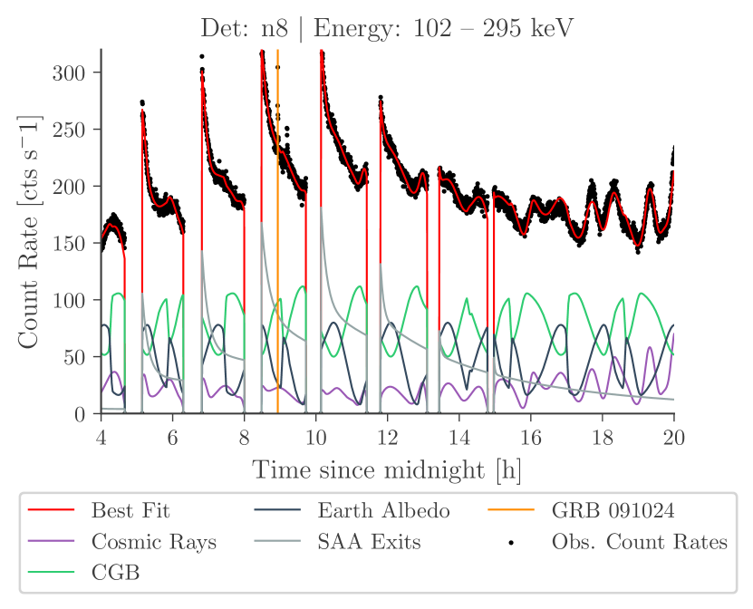
Figure 1: Data and background fit for the day of 24. Oct. 2009 for detector n8 in the reconstructed energy range of 102 – 295 keV with a time-bin size of 15 s. This includes the ultra-long GRB 091024: its GBM trigger at 08:56:01 is marked by a cyan line (Biltzinger et al., 2020).

All-sky monitoring instruments like Fermi-GBM are built to observe transient events in the $\gamma$-ray sky. Detecting these transients is a non-trivial task as they can be concealed by a strongly varying background (Fig. 1) which becomes especially important for weak and long duration transients. Swift/BAT complements its trigger algorithm with a hard X-ray transient monitor Krimm et al. (2013). In the case of Fermi-GBM, consisting of 12 NaI detectors and 2 BGO detectors and built primarily for detecting GRBs or similarly short-duration transients, two constraints come together: (i) the background at low energies is composed by a variety of bright sources, so in order to avoid triggering on those, the onboard trigger algorithm omits the lowest two energy channels covering 4–12 keV and 12–27 keV (Meegan et al., 2009); (ii) the temporal variations of the background in Fermi’s low-Earth orbit have a time-scale of 5–10 min, and consequently the longest onboard trigger timescale is set to 8.192 s (Meegan et al., 2009): thus, slow-rising or long-duration transients cannot be detected. The strongly varying background is the reason why there does not exist a pipeline searching for transients with variability slower than GRBs in the Fermi-GBM data. In all existing analysis tools, a polynom is fit to the background. As soon as the rise time of a transient source gets slower than a few minutes, the polynomial fit cannot distinguish anymore between background and new transient source.

The recent work by Antier et al. (2020) has tried to extend the covered energy range to 4 keV by applying a median-smoothing filter to remove the variable background and thus allow the independent identification of gamma-ray bursts including the detection of soft X-ray long transients. Antier et al. (2020) also applied an upper limit of 50 s to the allowed length of a transient signal, preventing its use for finding long duration transients. This method has similar shortfalls as a polynomial fit as it is unable to distinguish between a new source, e.g. a long duration transient, and background variations.

With the advent of our earlier developed physical background model (Biltzinger et al., 2020) these limitations (both, at low-energy as well as long durations) can be circumvented, motivating this work. The detection of transient events and GRBs can be formulated as the statistical problem of detecting significant variations (hereby change-points) in the light curves (or more generally time-series). The start- and endpoint of a transient are hereby estimated separately as two subsequent change-points in the time-series. This method is traditionally not among the standard methods described in the GRB trigger literature (Savchenko et al., 2012; Blackburn et al., 2015; Burns et al., 2019), but has recently been applied to the detection of GRBs in Antier et al. (2020). Here, we describe our extensions of this concept of change-point detection by incorporating a physical background model and combining the information of multiple dimensions, i.e. the information of the different detectors and different energy bands per time step.

2 Transient detection algorithm

2.1 Physical background model

For non-imaging instruments like GBM, the measured data are all-sky light curves with sources superimposed upon each other as a detector is scanning over the sky. Thus, in any analysis of temporal transients such as GRBs, GBM relies on the ability to separate source and background during any, or multiple, scan(s). This is classically done by identifying off-source regions in time, i.e. time intervals of the data stream when the source is not active, or not in the field-of-view of a scanning detector), and fitting smooth functions such as polynomials to each energy band’s temporally evolving signal and extrapolating this model into the on-source region (Pendleton et al., 1999; Greiner et al., 2016). This common approach is only suitable for transient events, which are short with respect to the timescale of the typical temporal variation of the background (about 10 min in case of Fermi-GBM). However, this leads to poor results for long duration events, as the extrapolation of the background can be inaccurate due to non-linear variations in the signal (Biltzinger et al., 2020). This can be overcome by constructing a physical model for the photon background seen by Fermi-GBM and fitting the normalization parameters of the individual background components (Fig. 1). This predictive background model is designed with a minimum number of free parameters that incorporated the physics of the source types, the response of the GBM detectors and the geometry and location of the spacecraft. This model should only fit the background and not also (long or slowly varying) transient signals, while allowing to extract the individual contributions of the different background sources. The background components can be categorized in two main classes: the photon components and the charged particle components. The sources in the first class produce a photon spectrum, which is measured directly in the detectors. The cosmic gamma-ray background, the Earth Albedo, point sources and the Sun are part of this class. The second class is characterized by charged particles that alter the background via direct energy deposit in the detectors or as secondary radiation after interaction with the satellite material. The origin of these charged particles are cosmic rays and those trapped in the South Atlantic Anomaly (SAA). The physical background model has been derived and explained in detail in Biltzinger et al. (2020).

Parameter estimation

These parameters of the physical background model can be inferred from the data using Bayesian methods. Biltzinger et al. (2020) estimated these parameters using the nested sampling algorithm MultiNest (Feroz et al., 2009) which provides good results for models with low to medium number of parameters. The parameter estimation can made more robust by fitting the light curves of multiple detectors and energy bands jointly. However, this increases the number of model parameters and the computational complexity significantly. To overcome this, the background model has been implemented in the probabilistic programming language Stan which is state-of-the-art for statistical modeling and high performance statistical computation (Carpenter et al., 2017). Full Bayesian inference is provided in Stan through two MCMC methods, the No-U-Turn sampler and an adaptive form of Hamiltonian Monte Carlo sampling Betancourt et al. (2017). Given its advanced sampling methods, Stan is able to efficiently sample from very high dimensional posterior distributions, like our multi-detector and multi-energy band background fits.

2.2 Change point detection

Many tasks in signal processing can be thought of as a search for an optimal partition of data measured over a time interval $I$. One such task is the identification of a change in the underlying state of a data generating process, possibly several times in the given time interval. These changes are commonly referred to as change-points and their detection has attracted researchers from the statistics and data mining communities for decades (Basseville & Nikiforov, 1995). Edge detection, segmentation, event detection and anomaly detection, are all similar methods and are occasionally applied to comparable problems (Aminikhanghahi & Cook, 2017). For our task of transient detection with GBM we use the data from the 12 NaI detectors with 8 energy channels each leading to a total of 96 individual time series, i.e. a time series with 96 dimensions, motivating the use of a dimensionality reduction method shortly introduced in the following subsections.

2.2.1 PELT - Pruned Exact Linear Time algorithm

A naive approach to find the optimal partitions consists of finding the optimal segmentation by iterating over all possible segmentations of the signal and returning the one that minimizes the objective function. The optimal partition algorithm introduced by Jackson et al. (2005) finds the global optimal segmentation of a time series with a computational cost of $\mathcal{O}(N^{2})$, the same as the greedy Bayesian Blocks algorithm. Killick et al. (2012) recently extended the optimal partition algorithm by introducing a pruning step within the dynamic program that reduces the computational cost to linear speed $\mathcal{O}(N)$ with mild assumptions, while not affecting the exactness of the resulting solution, hence the name Pruned Exact Linear Time (PELT). PELT leads to substantially more accurate segmentation than Binary Segmentation (Killick et al., 2012) while being asymptotically faster.

2.2.2 High-dimensional change-point detection

The previously discussed change-point detection algorithms work well in the uni-variate setting. Their extensions to multiple dimensions quickly become computationally intractable with increasing dimensionality (Scargle, 1998; Jackson et al., 2005; Fryzlewicz, 2014). This is commonly overcome by projecting the high-dimensional time-series to a lower dimensional one (Horváth & Hušková, 2012; Zhang et al., 2010; Enikeeva & Harchaoui, 2019). Grundy et al. (2020) introduced a new projection method that conserves changes in the first two moments and argues that the previous methods have been limited to detecting changes in a single parameter, usually the mean, which makes them impractical when multiple features of a time-series change. This projection is performed by constructing a p-dimensional time series as a series of p-dimensional column-vectors that are composed by the individual measurements at a time $t$. Each vector is then mapped to two values, the distances and the separation angle to a reference vector. For details on the choice of the reference vector and the mapping we refer to Grundy et al. (2020). As a result, by detecting changes in the distances and angles using a uni-variate change-point method like PELT, the change-points in p-dimensional series can be recovered Grundy et al. (2020).

2.2.3 Application to Fermi-GBM

In the case of transient detection with GBM a transient signal comes from a certain direction and would therefore leave a signal in multiple detectors and energy channels depending on the spectrum and the location of the source. This signal would be different in amplitude in the different detectors and would lead to a strong change in the angle measure and the distance measure shown in Fig. 2. In the case of a particle event there is a signal of similar strength in all detectors simultaneously, which increases the distance measure but the angle would stay approximately constant. This characteristic would make the angle measure more robust to false triggers on particle clouds. Nonetheless, transient signals are a change in the mean of the time series and investigation has shown that using both the distance and the angle measure provides empirically the best trigger results. Due to our aim of detecting soft and long-duration transients, we exclude the highest two energy bands from the trigger algorithm as they are dominated by background.

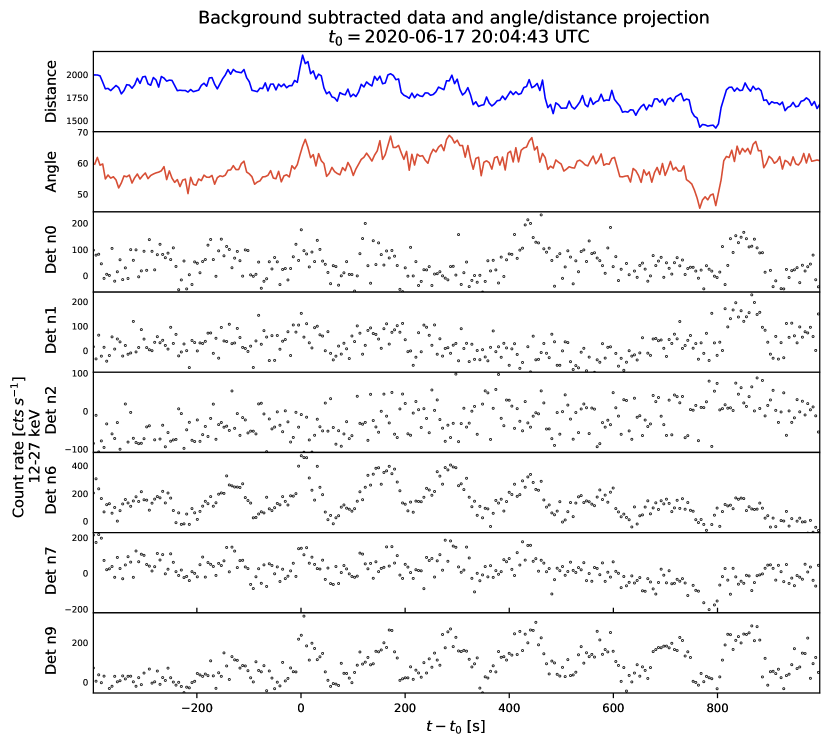
Figure 2: The background subtracted data of multiple detectors for the energy range 12–27 keV with a time binning of 5s in comparison to the projected angle and distance measure.

2.3 Source detection

Two consecutive change-points are combined as start and stop time to construct an source interval. For each source interval the significance is calculated by using the formula introduced by Vianello (2018) which applies some special treatment to avoid overestimating the significance of a candidate source by including the Gaussian error of the background fit performed using our model and applied to the unprojected data. In this case the estimated background $b$ follows a Gaussian distribution $\mathcal{N}(B,\sigma)$, with the true value $B$ and $\sigma$ as the error on the estimate. Many practitioners including the recent transient search by Antier et al. (2020) determine the significance with the formula $(n-b)/\sqrt{b}$, where $n$ is the number of observed counts. This introduces the assumption that $n$ follows a Poisson distribution with average $b$, which only holds if $B=b$; that the uncertainty on the background estimate is negligible $\sigma\rightarrow 0$ and that $n$ is large enough to converge to a Gaussian distribution with variance $\sqrt{b}$. Moreover, this form is a heuristically derived pseudo-statistic which has been shown to not map to an accurate significance distribution Li & Ma (1983). These assumptions are in most cases not justified and lead to an overestimated significance. The equation by Vianello (2018) (i.e. Eq. 15) for the significance in case of a measurement with Poisson noise and a background with Gaussian noise is:

$$S=\sqrt{2}\Bigg{[}n\log\bigg{(}\frac{n}{B_{0}^{mle}}\bigg{)}+\frac{(b-B_{0}^{mle})^{2}}{2\sigma^{2}}+B_{0}^{mle}-n\Bigg{]}^{\frac{1}{2}}$$ (1)

using the analytic solution $B_{0}^{mle}$ to the maximum likelihood estimate of the true background $B$.

For each source interval the significance is calculated for all detectors using eq. 1. Intervals with a significance of less than $5\,\sigma$ are discarded, whereas consecutive intervals with a significance higher than $5\,\sigma$ are combined. Each source interval is then ranked by its significance in the most significant detector. When overlapping intervals are encountered the interval with a lower significance is discarded.

To determine the active time used in the following localization, we determine for each detector the peak in excess counts and select an interval of $\pm 10$s around that peak. This time-interval has been selected as a trade-off between a longer time-interval for increased statistics and the systematic localization error introduced by the orbit of the satellite, i.e the boresight of Fermi (and thus that of most detectors) slewing with $1^{\circ}$ per 16s over the sky. For these time intervals we calculate the significance and store the most significant interval as active time for this trigger.

2.4 Localization

As Fermi-GBM is a non-imaging instrument, localizing transients is a challenging task. The applied method relies solely on the relative count rates observed by each of its 14 detectors. As the response of each GBM detector depends both on the incidence angle and energy of the detected photons, the measured count rate from a given transient source, depends on both the location and the physical spectrum of the source. The “BAyesian Location Reconstruction Of GRBs (BALROG)” method, introduced by Burgess et al. (2018) and studied systematically by Berlato et al. (2019) fits simultaneously for both sky location and spectrum of a source. This is done by constructing a full likelihood for the data set by combining the sky background from the physical background fit while propagating its errors, the instrument detector response matrices (DRMs), and a model for the transient source. The posterior samples are obtained by using MultiNest (Feroz et al., 2009), which implements a nested sampling algorithm.

3 Automatic detection pipeline

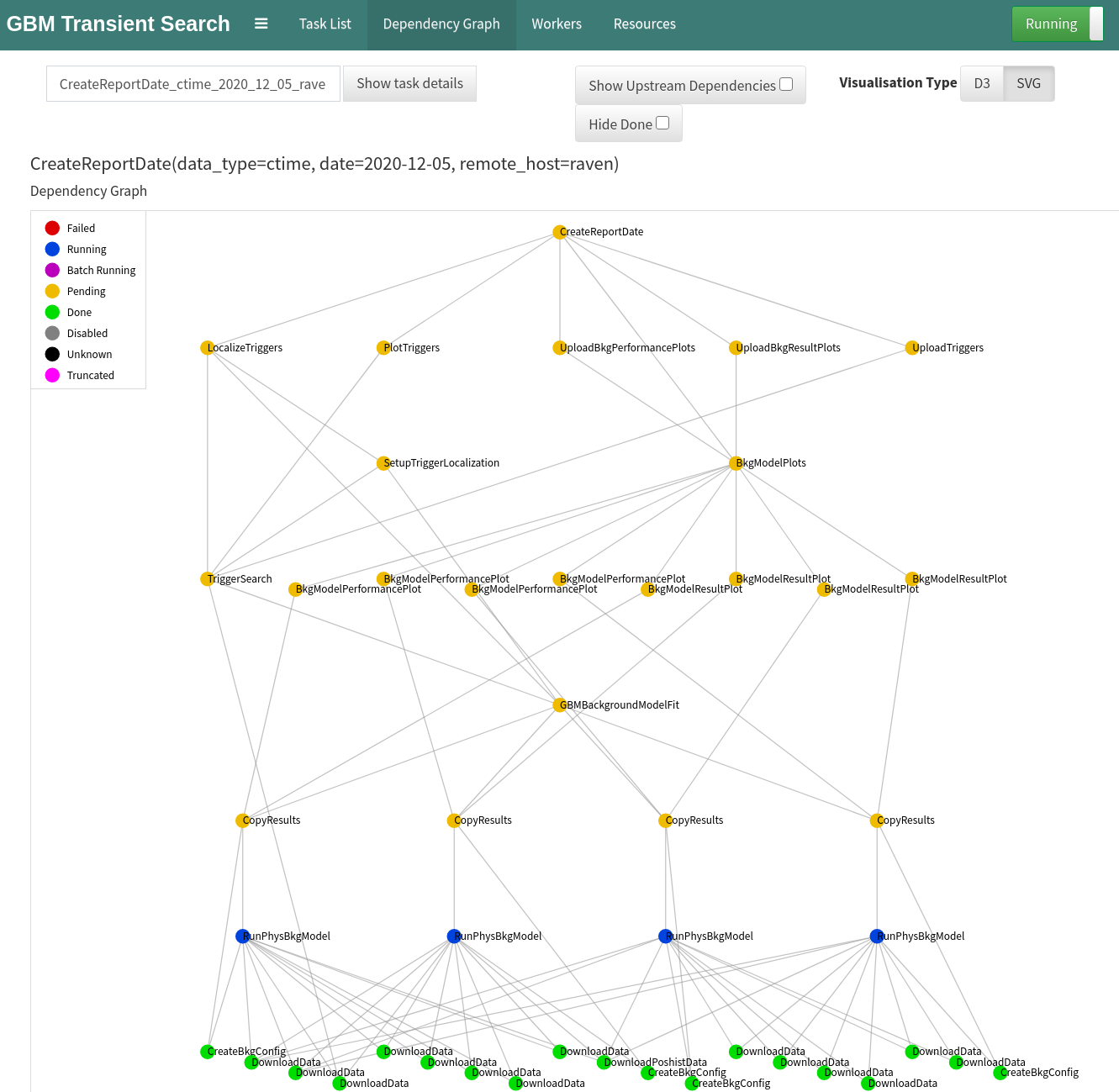
Figure 3: The dependency graph of the transient search pipeline, processing one day of data. Tasks that are already processed are marked with green circles, blue circles indicate tasks that are currently running and yellow circles indicate tasks that are pending due to missing dependencies. The processing starts at the bottom and the pipeline is currently running the fit of the background model (”RunPhysBkgModel”). The following step ”TriggerSearch” will run the change point detection (see subsection 2.2) and source detection (see subsection 2.3) of the transient detection algorithm. The subsequent ”SetupTriggerLocalization” step will dynamically add individual tasks for localization and spectral analysis (see subsection 2.4) for every found trigger. All found transient signals are then uploaded to the GRB Science Dashboard (https://grb.mpe.mpg.de).

To automatically search for transient signals, apart from the background modeling, the transient detection algorithm and the source localization, one key ingredient is still missing: the individual processing steps and their dependencies have to be orchestrated in a data analysis flow, that does not need human intervention. This can be done by building a processing pipeline that combines multiple processing steps and passes their outputs on to the next task. The developed method is a fully autonomous data analysis pipeline built with the luigi framework, that automatically downloads the satellite data as soon as they are available, runs all analysis steps and uploads a report to the GRB Science Dashboard (see Fig. 3). The GRB Science Dashboard provides an interactive interface to the detected transient signals and their localization and spectral analysis.

4 Simulations

4.1 Set-up

In order to evaluate the performance of the background model fit and the transient search algorithm, a simulation framework has been developed. An artificial data file is created containing the expected background fluctuations in the individual detectors and energy channels, by the following steps:

1. Instantiate the background model components using the location history file of the satellite and the time bins of one day as described in Biltzinger et al. (2020)

2. Keep the temporal evolution of the background components fixed

3. Set the normalization parameters of the background model components to known (simulated) values

4. Calculate the (time-dependent) flux of every component

5. Fold each flux through the detector responses for each time bin

6. Sum the contribution of all components

7. Sample from the Poisson distribution with k equal to the sum of components for each time bin

8. Store simulated count rates to FITS format like the original GBM data products

By fitting the physical background model to this artificial data set, the accuracy can be reviewed by comparing the posterior distribution over the parameters with the real (simulated) values.

To verify the performance of the trigger algorithm in a simulation, transient signals can be superimposed on the background. A realistic transient signal is simulated by defining a point source with a physical spectrum and a position on the sky, and folding the point source flux through a function defining the time evolution and thereby creating a transient point source. The flux of the transient point source is then folded through the detector responses taking into account the Earth occultation to obtain the simulated count rate per detector. The simulated data-set is created by adding this transient count rate to a simulated background model and subsequently adding Poisson noise.

In order to asses the sensitivity of the detection algorithm and the probability to detect a signal of given duration and significance, two different transient type light curves have been studied by simulating $N=2x10^{6}$ transient signals, as described in the next two subsections.

4.2 A single-pulse type transient

Figure 4: Light curves of a simulated transient point source with at Norris pulse time evolution on top of a simulated background. The count rate of the simulated transient is shown in orange, the background fit in red and the time interval detected by the algorithm is highlighted in gray. The projection to the distance and angle measure is shown as a reference in the upper two subplots.

For single-pulse type transients a simulated source has been created with a background-like spectrum (i.e. the sum of Earth Albedo and CGB given by two broken-powerlaws with $\alpha^{Earth}_{1}=-5$, $\alpha^{Earth}_{2}=1.72$ and $\alpha^{CGB}_{1}=1.32$, $\alpha^{CGB}_{2}=2.88$ (Ajello et al., 2008). The start time $t_{start}$ and a location of the transient on the sky have been sampled while making sure that the source was not occulted by the Earth. As time evolution of the transient we have applied the Norris pulse function

$$f_{\textrm{norris}}(t)=A\cdot exp\Bigg{(}2\sqrt{\frac{t_{\textrm{rise}}}{t_{\textrm{decay}}}}\,\Bigg{)}exp\Bigg{(}\dfrac{-t_{\textrm{rise}}}{t-t_{\textrm{start}}}-\frac{t-t_{\textrm{start}}}{t_{\textrm{decay}}}\Bigg{)},$$ (2)

which has been demonstrated to be a good representation of GRB pulses (Norris et al., 1996), by sampling values for $t_{rise}=t_{decay}$ from a Uniform distribution $\mathcal{U}\{0.1,200\}$. In Fig. 4 the simulated lightcurves of multiple detectors are shown for one simulation run. The simulated transient events are then binned in two dimensions by their duration and significance. This allows us to estimate the detection probability as

$$P=\frac{n_{\textrm{detected}}}{N}$$ (3)

for each bin individually and thereby as function of duration and significance of the signal. The error estimate for this probability can be obtained by using the frequentist formula

$$err=Z\sqrt{\frac{P(1-P)}{N}}$$ (4)

with $Z=1.96$ for the 95% error.

In Fig. 6 and Fig. 6 the detection probability and its error for signals with a duration of up to 1420 s are visualized. The view is clipped at a significance of $9\,\sigma$ for better visualization as stronger signals were detected in 100% of the trials. For signals with a duration of 100 s – 200 s and a significance between $4.5\,\sigma$ and $5\,\sigma$ we observe a detection probability of $P\approx 50\%$. For the same durations we note for a significance of $<4\,\sigma$ a probability of $P\approx 0\%$ and for a significance of $>5\,\sigma$ a probability of $P\approx 100\%$. From this point the detection probability is reducing with increasing signal duration for signals with a simulated significance close to the $5\,\sigma$ threshold.

Although this finding is at first counter-intuitive, this can be explained by the calculation of the significance being influenced by the Poisson noise especially in the tails of the pulse. As the Norris Pulse has a smooth rise and decay we set the active time of the pulse to the time interval where the pulse has an amplitude $f(t)>0.1\,A$, calculated the significance for this interval and assumed this as the simulated significance. Yet, it can lead to a higher significance than the simulated value, when the algorithm selects less of the peak, which increases the detection probability below the $5\,\sigma$ threshold. At the same time long duration signals with just above $5\,\sigma$ of simulated significance are smooth and consist of a slow rise and decay. The algorithm will detect the start of the transient with a delay for smooth signals, whereas the end of the signal is detected too early. Therefore, the method will not integrate over the entire signal, which can lead to a sub-threshold significance, and therefore to a neglected detection. This is balanced out by long duration signals with higher significances as they still pass the $5\,\sigma$ threshold even if we integrate only over some portion of the signal.

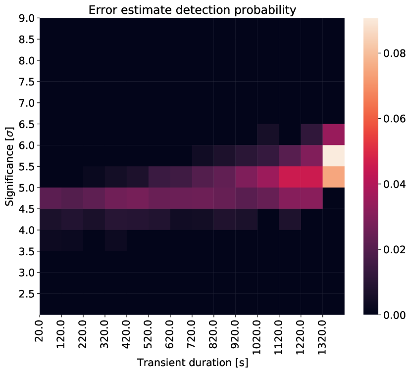
Figure 5: A 2D histogram showing the detection probability for a single-pulse type transient signal as function of its significance and duration.

Figure 6: The frequentist error estimate of the detection probabilities shown in Fig. 6

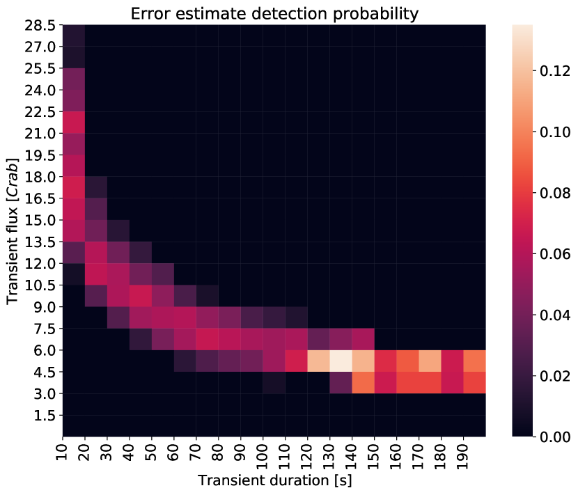
Figure 7: A 2D histogram showing the detection probability for a single-pulse type transient signal as function of the transient flux in units of mCrab and its duration for short duration signals between 10s and 200s.

Figure 8: The frequentist error estimate of the detection probabilities shown in Fig. 8

Figure 9: A 2D histogram showing the detection probability for a single-pulse type transient signal as function of the transient flux in units of mCrab and its duration for long duration signals between 100 s and 2000 s.

Figure 10: The frequentist error estimate of the detection probabilities shown in Fig. 10

To estimate the detection probability at a given flux of the transient, we will simulate the transient with the spectrum of the Crab nebula, a power-law with a spectral index of $2.106$ and a normalization of $9.71\;{\rm keV^{-1}cm^{-2}s^{-1}}$ (Madsen et al., 2017). The estimated detection probability plotted as a function of source flux in unites of Crab and the duration of the simulated transient is illustrated in Fig. 8 and Fig. 10. It is evident that with increasing transient duration, the required flux for a detection is decreasing. A detailed view for short duration signals is displayed in Fig. 8 and Fig. 8. It shows that for short duration signals of 10–25 s a $5\,\sigma$ detection requires a flux of up to 25 Crab. This could be at first surprising and should not be confused with the GRB detection sensitivity, but the reason for this is twofold: firstly, the time binning of the light curves in this simulation was 5 s, which as previously shown leads to a decrease in detection for signals with a duration of only a few time bins due to non-optimal time-selection. secondly, the significance of the detected signals is calculated taking into account the uncertainties of the physical background model, which slightly reduces the significance of a detection.

To put this flux into context we will compare it to the short GRB 170817A, which is considered to lay close to the detection threshold of GBM. The reported peak flux in the energy range of 10-1000 keV of this GRB was $(7.3\pm 2.5)\times 10^{-7}\;{\rm erg\ s^{-1}cm^{-2}}$ (Goldstein et al., 2017). This can be converted in units of Crab, which corresponds to a flux of $(14.4\pm 4.9)\textrm{ Crab}$. A short GRB of 10 s duration with the same flux as GRB 170817A would be detected with a 35% probability with our method optimized for long duration signals. It is likely that this can be further improved by using a finer time binning, which we leave for future optimization.

The detection threshold for long duration signals is illustrated in Figure 10. With increasing transient duration the flux required for a detection is decreasing. This is expected, because integration over long duration signals with the same flux leads to a higher significance than for short duration signals.

4.3 A switching-on transient

One potential application of the method developed in this work, is the detection of an astrophysical source going into outburst over a long period of time, which can last over multiple days. For simplification we assume the source to have a constant flux during the active time. Typically the flux of these sources is reported in units of the Crab nebula which is considered a standard candle in high-energy astrophysics. Therefore, we set the spectrum of the point source in this simulation to the spectrum of the Crab.

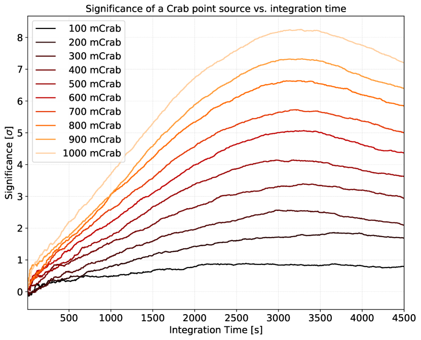
Figure 11: An illustration of the significance of a switching-on transient point source with a Crab spectrum as a function of integration time. The used detector sweeps over the point source with its optical axis at 1520 s. The start time of the integration has been chosen to maximise the overall significance. This represents the theoretical limit of significance that can be measured for this type of source, correctly incorporating the error of the background estimate.

To understand the required flux from this point source it is useful to first look at the ideal case, where one detector sweeps directly over the point source with its optical axis. In Fig. 11 the measured significance in this detector is shown as a function of the integration time. The start time of the integration has been set, by maximising the significance as a function of start time and integration time, and choosing the optimal value. The detector passes over the point sources with its optical axis at $t=1520$ s and the maximum significance is reached at an integration time of approximately $3200$ s. After this time the significance decreases as the point source is not visible by this detector anymore and we start integrating over background only. The peak differs slightly for each simulated curve due to the Poisson noise introduced in the simulated count rate. This shows that for a $5\sigma$ detection we need a point source with at least 600 mCrab and integrate over more than 3000 s. A point source with 500 mCrab does not reach the $5\sigma$ threshold even if we integrate over the entire visible orbit of approximately 3200 s.

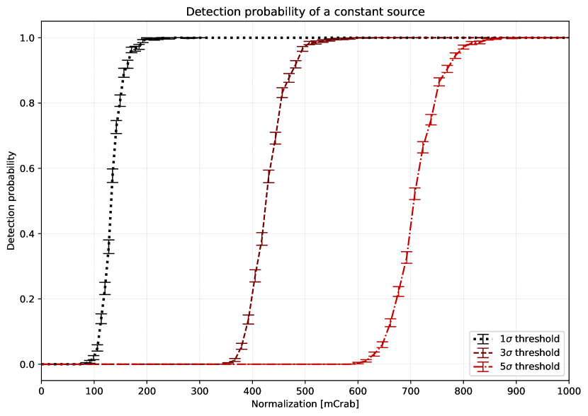
Figure 12: Detection probability for a switching-on transient source with a Crab spectrum as a function of flux at a detection threshold of $1\sigma$, $3\sigma$ and $5\sigma$.

To estimate the ability to detect this type of transient event with the automatic detection algorithm, an additional simulation has been performed. A transient point source that “turns on” instantly, stays constant over 24 hours and then stops stops instantly is simulated. Throughout the simulation the normalization has been sampled uniformly between 10 mCrab and 10 Crab. To marginalize over the detector configuration the position of the point sources has been sampled from a disc with 50 degree diameter. The detection probability can be calculated as introduced in the previous section by binning the simulated transients by the normalization and estimating the detection probability as $P=n_{\textrm{detected}}/N$.

The detection probability as a function of the point source flux is shown in Fig. 12 for a required detection significance of one sigma, three sigma, and five sigma. The algorithm shows a close to optimal performance, as the detection probability increases strongly starting at a flux level of 600 mCrab and reaches more than 95% at 800 mCrab. It has to be highlighted that during this simulation the location of the transient source is sampled randomly. Therefore, for only a fraction of simulated point sources a detectors sweeps over the source location on-axis. Furthermore the transient detection algorithm has not been tuned for this specific simulation but detected the start and integration time via the introduced change point detection method, running the (automated) detection pipeline. As we lower the required significance threshold we are able to detect events with a lower flux.

5 Physical Transients

To verify the performance of the pipeline with real data, two test runs have been performed spanning over approximately two months (2020/06/16 – 2020/07/14 and 2020/10/24 – 2020/11/17). The pipeline was run on chunks of data-sets of 1 full day, and the processing time per day was about 5 hrs. During this time the pipeline has run autonomous without a human in the loop. In this sample run the algorithm has successfully detected and localized more than 300 transient signals. A quick inspection revealed that only a handful of triggers could be classified as questionable. Using triggers with a $2\,\sigma$ localization error smaller than 25 deg (about 50% of all triggers), we find 12% of the triggers to be consistent with solar flares, 60% coming from known point sources such as the Crab, bright X-ray binaries such as Sco X-1 (dominatinating) or Cyg X-1, and 28% having no obvious high-energy counterpart in their error circle. Identifying these latter sources in the future will be a worthwhile subject of research.

On June 17, 2020, the transient search pipeline triggered three times on a pulsating signal.

1. 19:48:35 UTC with a duration of 665.6 s and a significance of $12.9\,\sigma$.

2. 20:04:53 UTC with a duration of 1593.6 s and a significance of $33.4\,\sigma$ (see Fig. 13).

3. 20:21:42 UTC with a duration of 153.6 s and a significance of $5.3\,\sigma$.

The automatic localization of the these three signals coincided at the location of $\textrm{RA}=142.2{\rm\;deg}$ and $\textrm{DEC}=-37.7{\rm\;deg}$ with a $2\,\sigma$ error circle of 56.4 degrees.

Figure 13: Observed data of GBM detector n6 around the time of the trigger.

To demonstrate the the capacity of this transient search method to find real physical signals, a manual analysis of this event has been performed to find a possible counterpart. In Fig. 13 the background subtracted data of detector n6 is shown around the trigger time of the second (strongest) trigger for the lowest three energy channels. A clear oscillating signal is visible with a periodicity of $T\approx 142\,s$.

In order to improve the error of the automatic localization of the pipeline, a manual localization has been performed. Multiple active time intervals have been selected covering multiple peaks, and for each interval a response is generated using gbm_drm_gen (Burgess et al., 2018). For each interval the count spectrum is generated and a joint BALROG fit is performed assuming a blackbody spectrum for the source, while linking the position parameters. In Fig. 14 the pair plot from this fit is shown, constraining the location of this source to $\textrm{RA}=137.5^{+2.2}_{-3.5}{\rm\;deg}$ and $\textrm{DEC}=-42.1^{+2.4}_{-2.3}{\rm\;deg}$.

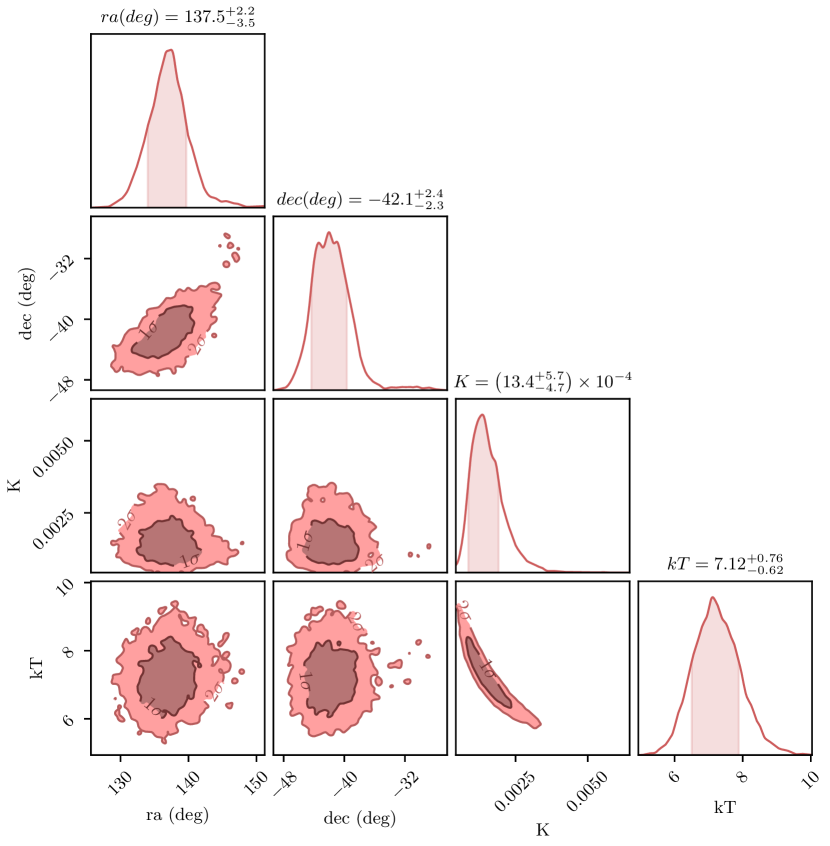
Figure 14: Result of the BALROG fit of the oscillating source with a blackbody spectrum using the data from multiple peaks.

To pinpoint the location and thereby establish the identification of this source we used the survey data of the Swift/BAT instrument. During this activity the Swift/BAT survey has performed multiple observations covering this source region. As Swift/BAT is more sensitive than GBM, the 5 min integration time of BAT survey mode should yield a detectable point source. These observations were processed using the batsurvey tool (Nasa High Energy Astrophysics Science Archive Research Center (2014), Heasarc), which directly produces a sky-map. Analysis of the observation 00013484027 lead to the detection of a point source at the position of $\textrm{RA}=135.5342{\rm\;deg}$ and $\textrm{Decl.}=-40.5619{\rm\;deg}$ with a S/N of 28.1 (see Fig. 15).

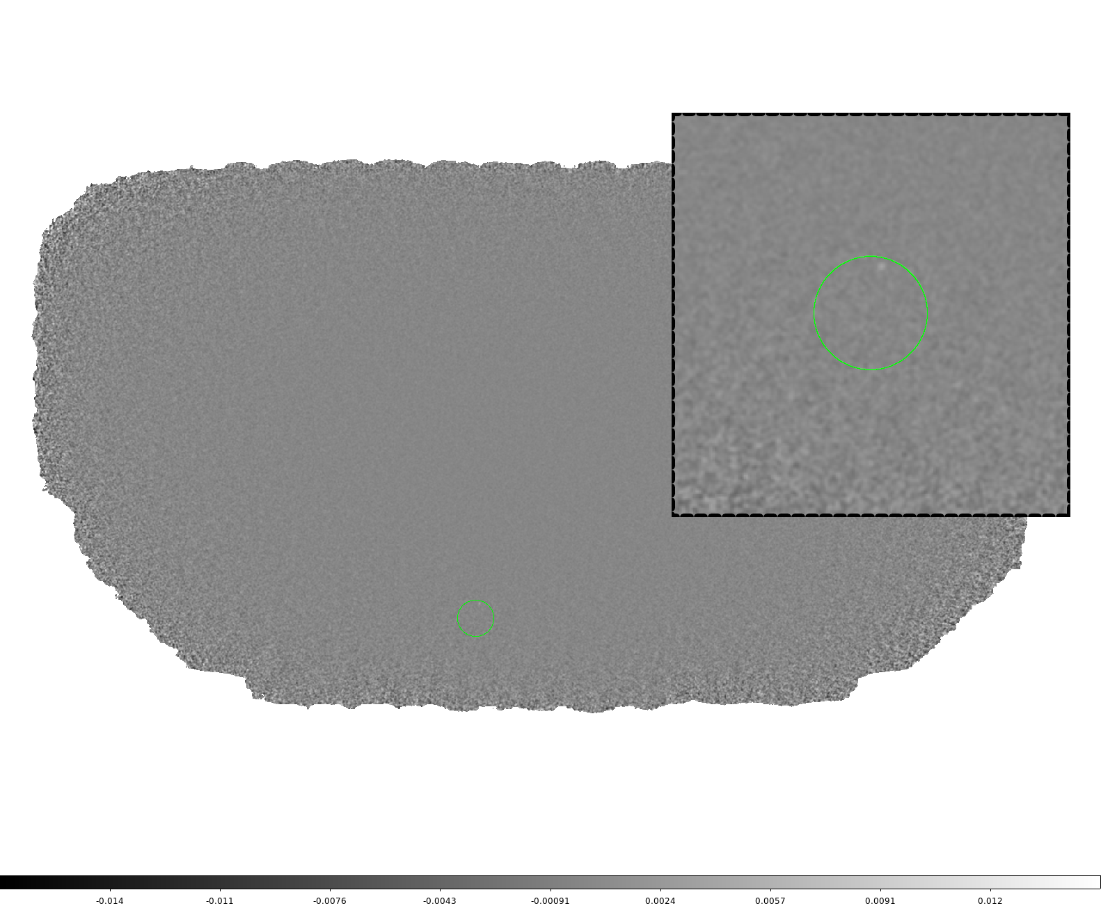
Figure 15: The sky-map from the Swift/BAT observation 00013484027 produced with the batsurvey tool. It shows the detected point source (white spot) that lies within the error region of the BALROG position (light green circle) of the transient Vela X-1. The color bar shows the intensity in units of counts/s.

The catalog of known X-ray sources reveals this source to be Vela X-1. Vela X-1, detected already with sounding rockets in the 1960ies (Chodil et al., 1967), and contained in the Uhuru satellite catalog as 4U 0900-40 (Forman et al., 1978), is a pulsing, eclipsing high-mass X-ray binary (HMXB) system that contains a neutron star and the supergiant star HD 77581 and is known for high energy flares (Kretschmar et al., 2019). The neutron star has a spin period of 283.53 s (Kreykenbohm et al., 2008) which is nicely seen even in the raw data (Fig. 13) and consistent with our periodicity of 142 s (we see emission from the north and the south pole of the neutron star separately). Due to inhomogeneities in the stellar wind this accretion rate is not constant leading to the observed transient nature of its overall flux. This remarkable result demonstrates the power of this novel transient detection algorithm.

6 Conclusions

The main objective of this study was to develop a novel method for the detection of untriggered long-duration transient events in the data of Fermi-GBM, longer than the 5–10 min of the time scale of the background variations. We applied a Bayesian framework to fit the physical background model, which allows for an effective decoupling of transient sources from the complex and varying background of the instrument. The proposed trigger algorithm combines the signal of multiple detectors and energy channels, providing an increased sensitivity in the detection of change-points. This new trigger algorithm is embedded into a data analysis pipeline that continuously searches the data stream of the satellite and automates the detection, localization, analysis and reporting of new transients. This work establishes a procedure of automatic detection of slowly rising, long-duration transients in Fermi-GBM data, and pinpointing the location with an imaging instrument like Swift/BAT in survey mode.

The result of our extensive simulations gives evidence for a near-optimal (close to 100% detection probability at $5\,\sigma$) trigger performance for long-duration signals. This allowed for the establishment of the source flux limit as a function of transient duration, required for detection. The fully automatic data analysis pipeline once enabled, allows the immediate use of this method for transient detections in the continuous data stream from the Fermi-GBM detector.

As a test example, we looked more closely at a triple trigger on June 17, 2020, and could identify it with enhanced X-ray emission from the known Vela X-1 pulsar.

The improvements made to the background model in form of multi-detector fits, new sampling methods, and adjusted parametrizations has not only enabled the transient detection in this work. It could also significantly contribute to future applications of the physical background model such as the measurements of individual model parameters over long time-spans.

The sensitivity for new transient detections could be improved by combining the search with other observations as is proposed by the “Astrophysical Multimessenger Observatory Network” (AMON). Joint detections of sub-threshold events in multiple instruments could significantly increase their plausibility.

The advances made in this study contribute to a greater understanding of long-duration transients and nurture the analyses in the multi-messenger era.