BagFlip: A Certified Defense against Data Poisoning

Abstract

Machine learning models are vulnerable to data-poisoning attacks, in which an attacker maliciously modifies the training set to change the prediction of a learned model. In a trigger-less attack, the attacker can modify the training set but not the test inputs, while in a backdoor attack the attacker can also modify test inputs. Existing model-agnostic defense approaches either cannot handle backdoor attacks or do not provide effective certificates (i.e., a proof of a defense). We present BagFlip, a model-agnostic certified approach that can effectively defend against both trigger-less and backdoor attacks. We evaluate BagFlip on image classification and malware detection datasets. BagFlip is equal to or more effective than the state-of-the-art approaches for trigger-less attacks and more effective than the state-of-the-art approaches for backdoor attacks.

1 Introduction

Recent works have shown that machine learning models are vulnerable to data-poisoning attacks, where the attackers maliciously modify the training set to influence the prediction of the victim model as they desire. In a trigger-less attack [42, 31, 24, 3, 1, 11], the attacker can modify the training set but not the test inputs, while in a backdoor attack [29, 34, 41, 30, 5, 21, 25, 27] the attacker can also modify test inputs. Effective attack approaches have been proposed for various domains such as image recognition [12], sentiment analysis [25], and malware detection [30].

Consider the malware detection setting. An attacker can modify the training data by adding a special signature—e.g., a line of code—to a set of benign programs. The idea is to make the learned model correlate the presence of the signature with benign programs. Then, the attacker can sneak a piece of malware past the model by including the signature, fooling the model into thinking it is a benign program. Indeed, it has been shown that if the model is trained on a dataset with only a few poisoned examples, a backdoor signature can be installed in the learned model [30, 27]. Thus, data-poisoning attacks are of great concern to the safety and security of machine learning models and systems, particularly as training data is gathered from different sources, e.g., via web scraping.

Ideally, a defense against data poisoning should fulfill the following desiderata: (1) Construct effective certificates (proofs) of the defense. (2) Defend against both trigger-less and backdoor attacks. (3) Be model-agnostic. It is quite challenging to fulfill all three desiderata; indeed, existing techniques are forced to make tradeoffs. For instance, empirical approaches [10, 40, 20, 26, 36, 13, 33, 9] cannot construct certificates and are likely to be bypassed by new attack approaches [32, 37, 16]. Some certified approaches [39, 35] provide ineffective certificates for both trigger-less and backdoor attacks. Some certified approaches [15, 19, 4, 28, 22, 38] provide effective certificates for trigger-less attacks but not backdoor attacks. Other certification approaches [14, 7, 23] are restricted to specific learning algorithms, e.g., decision trees.

This paper proposes BagFlip, a model-agnostic certified approach that uses randomized smoothing [6, 8, 18] to effectively defend against both trigger-less and backdoor attacks (Section 4). BagFlip uses a novel smoothing distribution that combines bagging of the training set and noising of the training data and the test input by randomly flipping features and labels.

Although both bagging-based and noise-based approaches have been proposed independently in the literature, combining them makes it challenging to compute the certified radius, i.e., the amount of poisoning a learning algorithm can withstand without changing its prediction.

To compute the certified radius precisely, we apply the Neyman–Pearson lemma to the sample space of BagFlip’s smoothing distribution. This lemma requires partitioning the outcomes in the sample space into subspaces such that the likelihood ratio in each subspace is a constant. However, because our sample space is exponential in the number of features, we cannot naively apply the lemma. To address this problem, we exploit properties of our smoothing distribution to design an efficient algorithm that partitions the sample space into polynomially many subspaces (Section 5). Furthermore, we present a relaxation of the Neyman–Pearson lemma that further speeds up the computation (Section 6). Our evaluation against existing approaches shows that BagFlip is comparable to them or more effective for trigger-less attacks and more effective for backdoor attacks (Section 7).

2 Related Work

Our model-agnostic approach BagFlip uses randomized smoothing to compute effective certificates for both trigger-less and backdoor attacks. BagFlip focuses on feature-and-label-flipping perturbation functions that modify training examples and test inputs. We discuss how existing approaches differ.

Some model-agnostic certified approaches can defend against both trigger-less and backdoor attacks but cannot construct effective certificates. Wang et al. [35], Weber et al. [39] defended feature-flipping poisoning attacks and $l_{2}$-norm poisoning attacks, respectively. However, their certificates are practically ineffective due to the curse of dimensionality [17].

Some model-agnostic certified approaches construct effective certificates but cannot defend against backdoor attacks. Jia et al. [15] proposed to defend against general trigger-less attacks, i.e., the attackers can add/delete/modify examples in the training dataset, by bootstrap aggregating (bagging). Chen et al. [4] extended bagging by designing other selection strategies, e.g., selecting without replacement and with a fixed probability. Rosenfeld et al. [28] defended against label-flipping attacks and instantiated their framework on linear classifiers. Differential privacy [22] can also provide probabilistic certificates for trigger-less attacks, but it cannot handle backdoor attacks, and its certificates are ineffective. Levine and Feizi [19] proposed a deterministic partition aggregation (DPA) to defend against general trigger-less attacks by partitioning the training dataset using a secret hash function. Wang et al. [38] further improved DPA by introducing a spread stage.

Other certified approaches construct effective certificates but are not model-agnostic. Jia et al. [14] provided deterministic certificates only for nearest neighborhood classifiers (kNN/rNN), but for both trigger-less and backdoor attacks. Meyer et al. [23], Drews et al. [7] provided deterministic certificates only for decision trees but against general trigger-less attacks.

3 Problem Definition

We take a holistic view of training and inference as a single deterministic algorithm $A$. Given a dataset $D=\{(\mathbf{x}_{1},y_{1}),\ldots,(\mathbf{x}_{n},y_{n})\}$ and a (test) input $\mathbf{x}$, we write $A(D,\mathbf{x})$ to denote the prediction of algorithm $A$ on the input $\mathbf{x}$ after being trained on dataset $D$.

We are interested in certifying that the algorithm will still behave “well” after training on a tampered dataset. Before describing what “well” means, to define our problem we need to assume a perturbation space—i.e., what possible changes the attacker could make to the dataset. Given a pair $(\mathbf{x},y)$, we write $\pi(\mathbf{x},y)$ to denote the set of perturbed examples that an attacker can transform the example $(\mathbf{x},y)$ into. Given a dataset $D$ and a radius $r\geq 0$, we define the perturbation space as the set of datasets that can be obtained by modifying up to $r$ examples in $D$ using the perturbation $\pi$:

$$S^{\pi}_{r}(D)=\left\{\{(\widetilde{\mathbf{x}}_{i},\widetilde{y}_{i})\}_{i}~{}\bigg{|}~{}\forall i.\ (\widetilde{\mathbf{x}}_{i},\widetilde{y}_{i})\in\pi(\mathbf{x}_{i},y_{i}),\ \sum_{i=1}^{n}\mathds{1}_{(\widetilde{\mathbf{x}}_{i},\widetilde{y}_{i})\neq(\mathbf{x}_{i},y_{i})}\leq r\right\}$$

Threat models. We consider two attacks: one where an attacker can perturb only the training set (a trigger-less attack) and one where the attacker can perturb both the training set and the test input (a backdoor attack). We assume a backdoor attack scenario where test input perturbation is the same as training one. If these two perturbation spaces can perturb examples differently, we can always over-approximate them by their union. In the following definitions, we assume that we are given a perturbation space $\pi$, a radius $r\geq 0$, and a benign training dataset $D$ and test input $\mathbf{x}$.

We say that algorithm $A$ is robust to a trigger-less attack on the test input $\mathbf{x}$ if $A$ yields the same prediction on the input $\mathbf{x}$ when trained on any perturbed dataset $\widetilde{D}$ and the benign dataset $D$. Formally,

$$\forall\widetilde{D}\in S^{\pi}_{r}(D).\ A(\widetilde{D},\mathbf{x})=A(D,\mathbf{x})$$ (1)

We say that algorithm $A$ is robust to a backdoor attack on the test input $\mathbf{x}$ if the algorithm trained on any perturbed dataset $\widetilde{D}$ produces the prediction $A(D,\mathbf{x})$ on any perturbed input $\widetilde{\mathbf{x}}$. Let $\pi(\mathbf{x},y)_{1}$ denote the projection of the perturbation space $\pi(\mathbf{x},y)$ onto the feature space (the attack can only backdoor features of the test input). Robustness to a backdoor attack is defined as

$$\forall\widetilde{D}\in S^{\pi}_{r}(D),\ \widetilde{\mathbf{x}}\in\pi(\mathbf{x},y)_{1}.\ A(\widetilde{D},\widetilde{\mathbf{x}})=A(D,\mathbf{x})$$ (2)

Given a large enough radius $r$, an attacker can always change enough examples and succeed at breaking robustness for either kind of attack. Therefore, we will focus on computing the maximal radius $r$, for which we can prove that Eq 1 and 2 hold for a given perturbation function $\pi$. We refer to this quantity as the certified radius. It is infeasible to prove Eq 1 and 2 by enumerating all possible $\widetilde{D}$ because $S^{\pi}_{r}(D)$ can be ridiculously large, e.g., $|S^{\pi}_{r}(D)|>10^{30}$ when $|D|=1000$ and $r=10$.

Defining the perturbation function. We have not yet specified the perturbation function $\pi$, i.e., how the attacker can modify examples. In this paper, we focus on the following perturbation spaces.

Given a bound $s\geq 0$, a feature-and-label-flipping perturbation, $\textsc{fl}_{s}$, allows the attacker to modify the values of up to $s$ features and the label in an example $(\mathbf{x},y)$, where $\mathbf{x}\in[K]^{d}$ (i.e., $\mathbf{x}$ is a $d$-dimensional feature vector with each dimension having $\{0,1,\ldots,K\}$ categories). Formally,

$$\textsc{fl}_{s}(\mathbf{x},y)=\{(\widetilde{\mathbf{x}},y^{\prime})\mid\|\mathbf{x}-\widetilde{\mathbf{x}}\|_{0}+\mathds{1}_{y\neq y^{\prime}}\leq s\},$$

There are two special cases of $\textsc{fl}_{s}$, a feature-flipping perturbation $\textsc{f}_{s}$ and a label-flipping perturbation l. Given a bound $s\geq 0$, $\textsc{f}_{s}$ allows the attacker to modify the values of up to $s$ features in the input $\mathbf{x}$ but not the label. l only allows the attacker to modify the label of a training example. Note that l cannot modify the test input’s features, so it can only be used in trigger-less attacks.

Example 3.1.

If $D$ is a binary-classification image dataset, where each pixel is either black or white, then the perturbation function $\textsc{f}_{1}$ assumes the attacker can modify up to one pixel per image.

The goal of this paper is to design a certifiable algorithm that can defend against trigger-less and backdoor attacks (Section 4) by computing the certified radius (Sections 5 and 6). Given a benign dataset $D$, our algorithm certifies that an attacker can perturb $D$ by some amount (the certified radius) without changing the prediction. Symmetrically, if we suspect that $D$ is poisoned, our algorithm certifies that even if an attacker had not poisoned $D$ by up to the certified radius, the prediction would have been the same. The two views are equivalent, and we use the former in the paper.

4 BagFlip: Dual-Measure Randomized Smoothing

Our approach, which we call BagFlip, is a model-agnostic certification technique. Given a learning algorithm $A$, we want to automatically construct a new learning algorithm $\bar{A}$ with certified poisoning-robustness guarantees (Eqs. 1 and 2). To do so, we adopt and extend the framework of randomized smoothing. Initially used for test-time robustness, randomized smoothing robustifies a function $f$ by carefully constructing a noisy version $\bar{f}$ and theoretically analyzing the guarantees of $\bar{f}$.

Our approach, BagFlip, constructs a noisy algorithm $\bar{A}$ by randomly perturbing the training set and the test input and invoking $A$ on the result. Formally, if we have a set of output labels $\mathcal{C}$, we define the smoothed learning algorithm $\bar{A}$ as follows:

$$\bar{A}(D,\mathbf{x})\triangleq\underset{y\in\mathcal{C}}{\mathrm{argmax}}\underset{\dot{D},\dot{\mathbf{x}}\sim\mu(D,\mathbf{x})}{\mathrm{Pr}}(A(\dot{D},\dot{\mathbf{x}})=y),$$ (3)

where $\mu$ is a carefully designed probability distribution—the smoothing distribution—over the training set and the test input ($\dot{D},\dot{\mathbf{x}}$ are a sampled dataset and a test input from the smoothing distribution).

We present two key contributions that enable BagFlip to efficiently certify robustness up to large poisoning radii. First, we define a smoothing distribution $\mu$ that combines bagging [15] of the training set $D$, and noising [35] of the training set and the test input $\mathbf{x}$ (done by randomly flipping features and labels). This combination, described below, allows us to defend against trigger-less and backdoor attacks. However, this combination also makes it challenging to compute the certified radius due to the combinatorial explosion of the sample space. Our second contribution is a partition strategy for the Neyman–Pearson lemma that results in an efficient certification algorithm (Section 5), as well as a relaxation of the Neyman–Pearson lemma that further speeds up certification (Section 6).

Smoothing distribution. We describe the smoothing distribution $\mu$ that defends against feature and label flipping. Given a dataset $D=\{(\mathbf{x}_{i},y_{i})\}$ and a test input $\mathbf{x}$, sampling from $\mu(D,\mathbf{x})$ generates a random dataset and test input in the following way: (1) Uniformly select $k$ examples from $D$ with replacement and record their indices as $w_{1},\ldots,w_{k}$. (2) Modify each selected example $(\mathbf{x}_{w_{i}},y_{w_{i}})$ and the test input $\mathbf{x}$ to $(\mathbf{x}_{w_{i}}^{\prime},y_{w_{i}}^{\prime})$ and $\mathbf{x}^{\prime}$, respectively, as follows: For each feature, with probability $1-\rho$, uniformly change its value to one of the other categories in $\{0,\ldots,K\}$. Randomly modify labels $y_{w_{i}}$ in the same way. In other words, each feature will be flipped to another value from the domain with probability $\gamma\triangleq\frac{1-\rho}{K}$, where $\rho\in[0,1]$ is the parameter controlling the noise level.

For $\textsc{f}_{s}$ (resp. l), we simply do not modify the labels (resp. features) of the $k$ selected examples.

Example 4.1.

Suppose we defend against $\textsc{f}_{1}$ in a trigger-less setting, then the distribution $\mu$ will not modify labels or the test input. Let $\rho=\frac{4}{5}$, $k=1$. Following Example 3.1, let the binary-classification image dataset $D=\{(\mathbf{x}_{1},y_{1}),(\mathbf{x}_{2},y_{2})\}$, where each image contains only one pixel. Then, one possible element of $\mu(D,\mathbf{x})$ can be the pair $(\{(\mathbf{x}_{2}^{\prime},y_{2})\},\mathbf{x})$, where $\mathbf{x}_{2}^{\prime}=\mathbf{x}_{2}$. The probability of this element is $\frac{1}{2}\times\rho=0.4$ because we uniformly select one out of two examples and do not flip any feature, that is, the single feature retains its original value.

5 A Precise Approach to Computing the Certified Radius

In this section, we show how to compute the certified radius of the smoothed algorithm $\bar{A}$ given a dataset $D$, a test input $\mathbf{x}$, and a perturbation function $\pi$. We focus on binary classification and provide the multi-class case in Appendix B.

Suppose that we have computed the prediction $y^{*}=\bar{A}(D,\mathbf{x})$. We want to show how many examples we can perturb in $D$ to obtain any other $\widetilde{D}$ so the prediction remains $y^{*}$. Specifically, we want to find the largest possible radius $r$ such that

$$\forall\widetilde{D}\in S^{\pi}_{r}(D),\ \widetilde{\mathbf{x}}\in\pi(\mathbf{x},y)_{1}.\ \underset{\dot{D},\dot{\mathbf{x}}\sim\mu(\widetilde{D},\widetilde{\mathbf{x}})}{\mathrm{Pr}}(A(\dot{D},\dot{\mathbf{x}})=y^{*})>0.5$$ (4)

We first show how to certify that Eq 4 holds for a given $r$ and then rely on binary search to compute the largest $r$, i.e., the certified radius. In Section 5.1, we present the Neyman–Pearson lemma to certify Eq 4 as it is a common practice in randomized smoothing. In Section 5.2, we show how to compute the certified radius for the distribution $\mu$ and the perturbation functions $\textsc{f}_{s},\textsc{fl}_{s}$, and l.

5.1 The Neyman–Pearson Lemma

Hereinafter, we simplify the notation and use $o$ to denote the pair $(\dot{D},\dot{\mathbf{x}})$ and $A(o)$ to denote the prediction of the algorithm training and evaluating on $o$. We further simplify the distribution $\mu(D,\mathbf{x})$ as $\mu$ and the distribution $\mu(\widetilde{D},\widetilde{\mathbf{x}})$ as $\widetilde{\mu}$. We define the performance of the smoothed algorithm $\bar{A}$ on dataset $D$, i.e., the probability of predicting $y^{*}$, as $p^{*}=\mathrm{Pr}_{o\sim\mu}(A(o)=y^{*})$.

The challenge of certifying Eq 4 is that we cannot directly estimate the performance of the smoothed algorithm on the perturbed data, i.e., $\mathrm{Pr}_{o\sim\widetilde{\mu}}(A(o)=y^{*})$, because $\widetilde{\mu}$ is universally quantified. To address this problem, we use the Neyman–Pearson lemma to find a lower bound $\mathrm{lb}$ for $\mathrm{Pr}_{o\sim\widetilde{\mu}}(A(o)=y^{*})$. We do so by constructing a worst-case algorithm $\bar{A^{?}}$ and distribution $\widetilde{\mu}$. Note that we add the superscript $?$ to denote a worst-case algorithm. Specifically, we minimize $\mathrm{Pr}_{o\sim\widetilde{\mu}}(A^{?}(o)=y^{*})$ while maintaining the algorithm’s performance on $\mu$, i.e., keeping $\mathrm{Pr}_{o\sim\mu}(A^{?}(o)=y^{*})=p^{*}$. We use $\mathcal{A}$ to denote the set of all possible algorithms. We formalize the computation of the lower bound $\mathrm{lb}$ as the following constrained minimization objective:

$$\mathrm{lb}\triangleq\min_{\bar{A^{?}}\in\mathcal{A}}\underset{o\sim\widetilde{\mu}}{\mathrm{Pr}}(A^{?}(o)=y^{*})\ \ \ \ s.t. \ \underset{o\sim\mu}{\mathrm{Pr}}(A^{?}(o)=y^{*})=p^{*}\text{ and }\widetilde{D}\in S^{\pi}_{r}(D),\widetilde{\mathbf{x}}\in\pi(\mathbf{x},y)_{1}$$ (5)

It is easy to see that $\mathrm{lb}$ is the lower bound of $\mathrm{Pr}_{o\sim\widetilde{\mu}}(A(o)=y^{*})$ in Eq. 4 because $\bar{A}\in\mathcal{A}$ and $\bar{A}$ satisfies the minimization constraint. Thus, $\mathrm{lb}>0.5$ implies the correctness of Eq. 4.

We show how to construct $\bar{A^{?}}$ and $\widetilde{\mu}$ greedily. For each outcome $o=(\dot{D},\dot{\mathbf{x}})$ in the sample space $\Omega$—i.e., the set of all possible sampled datasets and test inputs—we define the likelihood ratio of $o$ as $\eta(o)=p_{\mu}(o)/p_{\widetilde{\mu}}(o)$, where $p_{\mu}$ and $p_{\widetilde{\mu}}$ are the PMFs of $\mu$ and $\widetilde{\mu}$, respectively.

The key idea is as follows: We partition $\Omega$ into finitely many disjoint subspaces $\mathcal{L}_{1},\ldots,\mathcal{L}_{m}$ such that the likelihood ratio in each subspace $\mathcal{L}_{i}$ is some constant $\eta_{i}\in[0,\infty]$, i.e., $\forall o\in\mathcal{L}_{i}.\eta(o)=\eta_{i}$. We can sort and reorder the subspaces by likelihood ratios such that $\eta_{1}\geq\ldots\geq\eta_{m}$. We denote the probability mass of $\mu$ on subspace $\mathcal{L}_{i}$ as $p_{\mu}(\mathcal{L}_{i})$.

Example 5.1.

Suppose $p_{\mu}(o_{1}){=}\frac{4}{10},p_{\widetilde{\mu}}(o_{1}){=}\frac{4}{10},p_{\mu}(o_{2}){=}\frac{1}{10},p_{\widetilde{\mu}}(o_{2}){=}\frac{1}{10},p_{\mu}(o_{3}){=}\frac{4}{10},p_{\widetilde{\mu}}(o_{3}){=}\frac{1}{10}$, $p_{\mu}(o_{4}){=}\frac{1}{10},p_{\widetilde{\mu}}(o_{4}){=}\frac{4}{10}$. We can partition $o_{1}$ and $o_{2}$ into one subspace $\mathcal{L}$ because $\eta(o_{1}){=}\eta(o_{2}){=}1$.

The construction of the $\bar{A^{?}}$ that minimizes Eq. 5 is a greedy process, which iteratively assigns $A^{?}(o)=y^{*}$ for $\mathcal{L}_{1},\mathcal{L}_{2},\ldots$ until the budget $p^{*}$ is met. The worst-case $\widetilde{\mu}$ can also be constructed greedily by maximizing the top-most likelihood ratios, and we can prove that the worst-case happens when the difference between $\mu$ and $\widetilde{\mu}$ is maximized, i.e., $\widetilde{D}$ and $\widetilde{\mathbf{x}}$ are maximally perturbed. The following theorem adapts the Neyman–Pearson lemma to our setting.

Theorem 5.1 (Neyman–Pearson Lemma for $\textsc{fl}_{s},\textsc{f}_{s},\textsc{l}$).

Let $\widetilde{D}$ and $\widetilde{\mathbf{x}}$ be a maximally perturbed dataset and test input, i.e., $|\widetilde{D}\setminus D|=r$, $\|\widetilde{\mathbf{x}}-\mathbf{x}\|_{0}=s$, and $\|\widetilde{\mathbf{x}}_{i}-\mathbf{x}_{i}\|_{0}+\mathds{1}_{\widetilde{y}_{i}\neq y_{i}}=s$, for each perturbed example $(\widetilde{\mathbf{x}}_{i},\widetilde{y}_{i})$ in $\widetilde{D}$. Let $i_{\mathrm{lb}}\triangleq\mathrm{argmin}_{{i\in[1,m]}}\sum_{j=1}^{i}p_{\mu}(\mathcal{L}_{j})\geq p^{*}$. Then, $\mathrm{lb}=\sum_{j=1}^{i_{\mathrm{lb}}-1}p_{\widetilde{\mu}}(\mathcal{L}_{j})+\left(p^{*}-\sum_{j=1}^{i_{\mathrm{lb}}-1}p_{\mu}(\mathcal{L}_{j})\right)/\eta_{i_{\mathrm{lb}}}$.

We say that $\mathrm{lb}$ is tight due to the existence of the minimizer $\bar{A^{?}}$ and $\widetilde{\mu}$ (see Appendix B).

Example 5.2.

Following Example 5.1, suppose $\Omega=\{o_{1},\ldots,o_{4}\}$ and we partition it into $\mathcal{L}_{1}=\{o_{3}\},\mathcal{L}_{2}=\{o_{1},o_{2}\}$, $\mathcal{L}_{3}=\{o_{4}\}$, and $\eta_{1}=4,\eta_{2}=1,\eta_{3}=0.25$. Let $p^{*}=0.95$, then we have $i_{\mathrm{lb}}=3$ and $\mathrm{lb}=0.1+0.5+(0.95-0.4-0.5)/0.25=0.8$.

5.2 Computing the Certified Radius of BagFlip

Computing the certified radius boils down to computing $\mathrm{lb}$ in Eq 5 using Theorem 5.1. To compute $\mathrm{lb}$ for BagFlip, we address the following two challenges: 1) The argmin of computing $i_{\mathrm{lb}}$ and the summation of $\mathrm{lb}$ in Theorem 5.1 depend on the number of subspaces $\mathcal{L}_{j}$’s. We design a partition strategy that partitions $\Omega$ into a polynomial number of subspaces ($O(k^{2}d)$). Recall that $k$ is the size of the bag sampled from $D$ and $d$ is the number of features. 2) In Theorem 5.1, $\mathrm{lb}$ depends on $p_{\mu}(\mathcal{L}_{j})$, which according to its definition (Eq 8) can be computed in exponential time ($O(kd^{2k})$). We propose an efficient algorithm that computes these two quantities in polynomial time ($O(d^{3}+k^{2}d^{2})$).

We first show how to address these challenges for $\textsc{f}_{s}$ and then show how to handle $\textsc{fl}_{s}$ and l.

Partition strategy. We partition the large sample space $\Omega$ into disjoint subspaces $\mathcal{L}_{c,t}$ that depend on $c$, the number of perturbed examples in the sampled dataset, and $t$, the number of features the clean data and the perturbed data differ on with respect to the sampled data. Intuitively, $c$ takes care of the bagging distribution and $t$ takes care of the feature-flipping distribution. Formally,

$$\mathcal{L}_{c,t}=\{ (\{(\mathbf{x}_{w_{i}}^{\prime},y_{w_{i}})\}_{i},\mathbf{x}^{\prime})\mid$$

$$\sum_{i=1}^{k}\mathds{1}_{\mathbf{x}_{w_{i}}\neq\widetilde{\mathbf{x}}_{w_{i}}}=c,$$ (6)

$$\underbrace{\left(\sum_{i=1}^{k}\|\mathbf{x}_{w_{i}}^{\prime}-\mathbf{x}_{w_{i}}\|_{0}+\|\mathbf{x}^{\prime}-\mathbf{x}\|_{0}\right)}_{\Delta}-\underbrace{\left(\sum_{i=1}^{k}\|\mathbf{x}_{w_{i}}^{\prime}-\widetilde{\mathbf{x}}_{w_{i}}\|_{0}+\|\mathbf{x}^{\prime}-\widetilde{\mathbf{x}}\|_{0}\right)}_{\widetilde{\Delta}}=t\}$$ (7)

Eq 6 means that there are $c$ perturbed indices sampled in $o$. $\Delta$ (and $\widetilde{\Delta}$) in Eq 7 counts how many features the sampled and the clean data (the perturbed data) differ on. The number of possible subspaces $\mathcal{L}_{c,t}$, which are disjoint by definition, is $O(k^{2}d)$ because $0\leq c\leq k$ and $|t|\leq(k+1)d$.

The next theorems show how to compute the likelihood ratio of $\mathcal{L}_{c,t}$ and $p_{\mu}(\mathcal{L}_{c,t})$.

Theorem 5.2 (Compute $\eta_{c,t}$).

$\eta_{c,t}=p_{\mu}(\mathcal{L}_{c,t})/p_{\widetilde{\mu}}(\mathcal{L}_{c,t})=(\gamma/\rho)^{t}$, where $\gamma$ and $\rho$ are parameters controlling the noise level in BagFlip’s smoothing distribution $\mu$.

Theorem 5.3 (Compute $p_{\mu}(\mathcal{L}_{c,t})$).

$$p_{\mu}(\mathcal{L}_{c,t})=\underset{o\sim\mu}{\mathrm{Pr}}(o\text{ satisfies Eq~{}\ref{eq:Ldef1}})\underset{o\sim\mu}{\mathrm{Pr}}(o\text{ satisfies Eq~{}\ref{eq:Ldef3}}\mid o\text{ satisfies Eq~{}\ref{eq:Ldef1}}),$$

where $\mathrm{Pr}_{o\sim\mu}(o\text{ satisfies Eq~{}\ref{eq:Ldef1}})=\mathrm{Binom}(c;k,\frac{r}{n})$ is the PMF of the binomial distribution and

$$T(c,t)\triangleq\underset{o\sim\mu}{\mathrm{Pr}}(o\text{ satisfies Eq~{}\ref{eq:Ldef3}}\mid o\text{ satisfies Eq~{}\ref{eq:Ldef1}})=\sum_{\begin{subarray}{c}0\leq\Delta_{i},\widetilde{\Delta}_{i}\leq d,\forall i\in[0,d]\\ \Delta_{0}-\widetilde{\Delta}_{0}+\ldots+\Delta_{c}-\widetilde{\Delta}_{c}=t\end{subarray}}\prod_{i=0}^{c}L(\Delta_{i},\widetilde{\Delta}_{i};s,d)\gamma^{\Delta_{i}}\rho^{d-\Delta_{i}},$$ (8)

where $L(\Delta,\widetilde{\Delta};s,d)$ is the same quantity defined in Lee et al. [18].

Remark 5.1.

We can compute $p_{\widetilde{\mu}}(\mathcal{L}_{c,t})$ as $\eta_{c,t}p_{\mu}(\mathcal{L}_{c,t})$ by the definition of $\eta_{c,t}$.

Efficient algorithm to compute Eq 8. The following algorithm computes $T(c,t)$ efficiently in time $O(d^{3}+k^{2}d^{2})$: 1) Computing $L(u,v;s,d)$ takes $O(d^{3})$ (see Appendix C for details). 2) Computing $T(0,t)$ by the definition in Eq 8 takes $O(kd^{2})$. 3) Computing $T(c,t)$ for $c\geq 1$ by the following equation takes $O(k^{2}d^{2})$.

$$T(c,t)=\sum_{t_{1}=\max(-d,t-cd)}^{\min(d,t+cd)}T(c-1,t-t_{1})T(0,t_{1})$$ (9)

Theorem 5.4 (Correctness of the Algorithm).

$T(c,t)$ in Eq 9 is the same as the one in Eq 8.

The above computation still applies to perturbation function $\textsc{fl}_{s}$ and l. Intuitively, flipping the label can be seen as flipping another dimension in the input features (Details in Section B.1).

Practical perspective. For each test input $\mathbf{x}$, we need to estimate $p^{*}$ for the smoothed algorithm $\bar{A}$ given the benign dataset $D$. We use Monte Carlo sampling to compute $p^{*}$ by the Clopper-Pearson interval. We also reuse the trained algorithms for each test input in the test set by using Bonferroni correction. We memoize the certified radius by enumerating all possible $p^{*}$ beforehand so that checking Eq 4 can be done in constant time in an online scenario (details in Section B.2). We cannot use floating point numbers because some intermediate values are too small to store in the floating point number format. Instead, we use rational numbers which represent the nominator and denominator in large numbers.

6 An Efficient Relaxation for Computing a Certified Radius

Theorem 5.1 requires computing the likelihood ratio of a large number of subspaces $\mathcal{L}_{1},\ldots,\mathcal{L}_{m}$. We propose a generalization of the Neyman–Pearson lemma that underapproximates the subspaces by a small subset and computes a lower bound $\mathrm{lb}_{\delta}$ for $\mathrm{lb}$. We then show how to choose a subset of subspaces that yields a tight underapproximation.

A relaxation of the Neyman–Pearson lemma. The key idea is to use Theorem 5.1 to examine only a subset of the subspaces $\{\mathcal{L}_{i}\}_{i}$. Suppose that we partition the subspaces $\{\mathcal{L}_{i}\}_{i}$ into two sets $\{\mathcal{L}_{i}\}_{i\in B}$ and $\{\mathcal{L}_{i}\}_{i\not\in B}$, using a set of indices $B$. We define a new lower bound $\mathrm{lb}_{\delta}$ by applying Theorem 5.1 to the first group $\{\mathcal{L}_{i}\}_{i\in B}$ and underapproximating $p^{*}$ in Theorem 5.1 as $p^{*}-\sum_{i\notin B}p_{\mu}(\mathcal{L}_{i})$. Intuitively, the underapproximation ensures that any subspace in $\{\mathcal{L}_{i}\}_{i\not\in B}$ will not contribute to the lower bound, even though these subspaces may have contributed to the precise $\mathrm{lb}$ computed by Theorem 5.1.

The next theorem shows that $\mathrm{lb}_{\delta}$ will be smaller than $\mathrm{lb}$ by an error term $\delta$ that is a function of the partition $B$. The gain is in the number of subspaces we have to consider, which is now $|B|$.

Theorem 6.1 (Relaxation of the Lemma).

Define $\mathrm{lb}$ for the subspaces $\mathcal{L}_{1},\ldots,\mathcal{L}_{m}$ as in Theorem 5.1. Define $\mathrm{lb}_{\delta}$ for $\{\mathcal{L}_{i}\}_{i\in B}$ as in Theorem 5.1 by underapproximating $p^{*}$ as $p^{*}-\sum_{i\notin B}p_{\mu}(\mathcal{L}_{i})$, then we have Soundness: $\mathrm{lb}_{\delta}\leq\mathrm{lb}$ and $\delta$-Tightness: Let $\delta\triangleq\sum_{i\notin B}p_{\widetilde{\mu}}(\mathcal{L}_{i})$, then $\mathrm{lb}_{\delta}+\delta\geq\mathrm{lb}$.

Example 6.1.

Consider $\mathcal{L}_{1},\mathcal{L}_{2}$, and $\mathcal{L}_{3}$ from Example 5.2. If we set $B=\{1,2\}$ and underapproximate $p^{*}$ as $p^{*}-p_{\mu}(\mathcal{L}_{3})=0.85$, then we have $\mathrm{lb}_{\delta}=0.1+(0.85-0.4)/1=0.55$, which can still certify Eq. 4. However, $\mathrm{lb}_{\delta}$ is not close to the original $\mathrm{lb}=0.8$ because the error $\delta=0.4$ is large in this example. Next, we will show how to choose $B$ as small as possible while still keeping $\delta$ small.

Speeding up radius computation. The total time for computing $\mathrm{lb}$ consists of two parts, (1) the efficient algorithm (Eq 9) computes $T(c,t)$ in $O(d^{3}+k^{2}d^{2})$, and (2) Theorem 5.1 takes $O(k^{2}d)$ for a given $p^{*}$ because there are $O(k^{2}d)$ subspaces. Even though we have made the computation polynomial by the above two techniques in Section 5.2, it can still be slow for large bag sizes $k$, which can easily be in hundreds or thousands.

We will apply Theorem 6.1 to replace the bag size $k$ with a small constant $\kappa$. Observe that $p_{\mu}(\mathcal{L}_{c,t})$ and $p_{\widetilde{\mu}}(\mathcal{L}_{c,t})$, as defined in Section 5.2, are negligible for large $c$, i.e., the number of perturbed indices in the smoothed dataset. Intuitively, if only a small portion of the training set is perturbed, it is unlikely that we select a large number of perturbed indices in the smoothed dataset. We underapproximate the full subspaces to $\{\mathcal{L}_{c,t}\}_{(c,t)\in B}$ by choosing the set of indices $B=\{(c,t)\mid c\leq\kappa,|t|\leq(c+1)d\}$, where $\kappa$ is a constant controlling the error $\delta$, which can be computed as $\delta=\sum_{i\notin B}p_{\widetilde{\mu}}(\mathcal{L}_{i})=1-\sum_{c=0}^{\kappa}\mathrm{Binom}(c;k,\frac{r}{n})$. Theorem 6.1 reduces the number of subspaces to $|B|=O(\kappa^{2}d)$. As a result, all the $k$ appearing in previous time complexity can be replaced with $\kappa$.

Example 6.2.

Suppose $k=150$ and $\frac{r}{n}=0.5\%$, choosing $\kappa=6$ leads to $\delta=1.23\times 10^{-5}$. In other words, it speeds up almost 625X for computing $T(c,t)$ and for applying Theorem 5.1.

7 Experiments

The implementation of BagFlip is publicly available. In this section, we evaluate BagFlip against trigger-less and backdoor attacks and compare BagFlip with existing work. Note that we apply the relaxation in Section 6 to BagFlip in all experiments and set $\delta=10^{-4}$.

Datasets. We conduct experiments on MNIST, CIFAR10, EMBER [2], and Contagio (http://contagiodump.blogspot.com). MNIST and CIFAR10 are datasets for image classification. EMBER and Contagio are datasets for malware detection, where data poisoning can lead to disastrous security consequences. To align with existing work, we select subsets of MNIST and CIFAR10 as MNIST-17, MNIST-01, and CIFAR10-02 in some experiments, e.g., MNIST-17 is a subset of MNIST with classes 1 and 7. We discretize all the features when applying BagFlip. We use clean datasets except in the comparison with RAB [39], where we follow their experimental setup and use backdoored datasets generated by BadNets [12]. A detailed description of the datasets is in Section E.1.

Models. We train neural networks for MNIST, CIFAR10, EMBER and random forests for Contagio. Unless we specifically mention the difference in some experiments, whenever we compare BagFlip to an existing work, we will use the same network structures, hyper-parameters, and data augmentation as the compared work, and we train $N=1000$ models and set the confidence level as $0.999$ for each configuration. All the configurations we used can be found in the implementation.

Metrics. For each test input $(\mathbf{x}_{i},y_{i})$, algorithm $\bar{A}$ will predict a label and the certified radius $r_{i}$. Assuming that the attacker had poisoned $R\%$ of the examples in the training set, we define certified accuracy as the percentage of test inputs that are correctly classified and their certified radii are no less than $R$, i.e., $\sum_{i=1}^{m}\mathds{1}_{\bar{A}(D,\mathbf{x}_{i})=y_{i}\wedge\frac{r_{i}}{n}\geq R\%}$. We define normal accuracy as the percentage of test inputs that are correctly classified, i.e., $\sum_{i=1}^{m}\mathds{1}_{\bar{A}(D,\mathbf{x}_{i})=y_{i}}$.

7.1 Defending Against Trigger-less Attacks

Two model-agnostic certified approaches, Bagging [15] and LabelFlip [28], can defend against trigger-less attacks. BagFlip outperforms LabelFlip (comparison in Section E.2). We evaluate BagFlip on the perturbation $\textsc{f}_{s}$ using MNIST, CIFAR10, EMBER, and Contagio and compare BagFlip to Bagging. We provide comparisons with Bagging on other perturbation spaces in Section E.2.

We present BagFlip with different noise levels (different probabilities of $\rho$ when flipping), denoted as BagFlip-$\rho$. When comparing to Bagging, we use the same $k$, the size of sampled datasets, for a fair comparison. Furthermore, we tune the parameter $k$ in Bagging to match the normal accuracy with the BagFlip-$\rho$ setting, and denote this setting as Bagging-$\rho$. Concretely, we set $k=100,1000,300,30$ for MNIST, CIFAR10, EMBER, and Contagio respectively when comparing to Bagging. We tune $k=80,280$ for Bagging-0.9 on MNIST and Bagging-0.95 on EMBER, respectively. And we set $k=50$ for MNIST when comparing to LabelFlip.

Figure 1: Comparison to Bagging on MNIST and EMBER, showing the certified accuracy at different poisoning amounts $R$. For MNIST: $a=0.9$ and $b=0.8$. For EMBER: $a=0.95$ and $b=0.9$.

Table 1: Certified accuracy on MNIST and EMBER with perturbations $\textsc{f}_{1}$ and $\textsc{f}_{\infty}$. Note that the certified accuracies are the same poisoning amount $R=0$ because we reuse the trained models.

		$\textsc{f}_{1}$						$\textsc{f}_{\infty}$
MNIST	$R$	$0$	$0.5$	$1.0$	$1.5$	$2.0$	$2.5$	$0$	$0.13$	$0.27$	$0.40$	$0.53$	$0.83$
	Bagging	94.54	66.84	0	0	0	0	94.54	90.83	85.45	77.61	61.46	0
	Bagging-0.9	93.58	71.11	0	0	0	0	93.58	89.80	84.92	78.60	68.11	0
	BagFlip-0.9	93.62	75.95	27.73	4.02	0	0	93.62	89.45	83.62	74.19	56.65	0
	BagFlip-0.8	90.72	73.94	46.20	33.39	24.23	5.07	90.72	84.11	74.50	60.56	39.21	0
EMBER	$R$	$0$	$0.07$	$0.13$	$0.20$	$0.27$	$0.33$	$0$	$0.05$	$0.10$	$0.15$	$0.20$	$0.25$
	Bagging	82.65	75.11	66.01	0	0	0	82.65	76.30	72.94	61.78	0	0
	Bagging-0.95	79.06	75.32	70.19	14.74	0	0	79.06	76.23	73.50	68.45	14.74	0
	BagFlip-0.95	79.17	75.93	69.30	57.36	0	0	79.17	76.83	72.41	62.04	30.36	0
	BagFlip-0.9	78.18	69.40	62.11	41.21	13.89	1.70	78.18	70.79	63.16	41.24	11.64	0

Comparison to Bagging. Bagging on a discrete dataset is a special case of BagFlip when $\rho=1$, i.e., no noise is added to the dataset. (We present the results of bagging on the original dataset (undiscretized) in Section E.2). Table 1 and Fig 1 show the results of BagFlip and Bagging on perturbations $\textsc{f}_{1}$ and $\textsc{f}_{\infty}$ over MNIST and EMBER. The results of CIFAR10 and Contagio are similar and shown in Section E.2. $\textsc{f}_{1}$ only allows the attacker to modify one feature in each training example, and $\textsc{f}_{\infty}$ allows the attacker to modify each training example arbitrarily without constraint. For $\textsc{f}_{1}$ on MNIST, BagFlip-0.9 performs better than Bagging after $R=0.19$ and BagFlip-0.8 still retains non-zero certified accuracy at $R=2.5$ while Bagging’s certified accuracy drops to zero after $R=0.66$. We observe similar results on EMBER for $\textsc{f}_{1}$ in Table 1, except $R=0.13$ when compared to Bagging-0.95. We argue that it is possible to tune a best combination of $k$ and $\rho$ for BagFlip, like we tune $k$ for Bagging-0.95, and achieve a better result while maintaining similar normal accuracy. However, we do not conduct hyperparameter-tuning for BagFlip because of its computation cost. BagFlip achieves higher certified accuracy than Bagging when the poisoning amount is large for $\textsc{f}_{1}$.

For $\textsc{f}_{\infty}$ on MNIST, Bagging performs better than BagFlip across all $R$ because the noise added by BagFlip to the training set hurts the accuracy. However, we find that the noise added by BagFlip helps it perform better for $\textsc{f}_{\infty}$ on EMBER. Specifically, BagFlip achieves similar certified accuracy as Bagging at small radii and BagFlip performs better than Bagging after $R=0.15$. Bagging achieves higher certified accuracy than BagFlip for $\textsc{f}_{\infty}$. Except in EMBER, BagFlip achieves higher certified accuracy than Bagging when the amount of poisoning is large.

Figure 2: (a) BagFlip-0.8 on MNIST against $\textsc{f}_{s}$ with different $s$. $s=8$ almost overlaps with $s=\infty$. (b) BagFlip-0.8 on MNIST and BagFlip-0.9 on Contagio against backdoor attack with $\textsc{f}_{1}$. Dashed lines show normal accuracy.

We also study the effect of different $s$ in the perturbation function $\textsc{f}_{s}$. Figure 2 shows the result of BagFlip-0.8 on MNIST. BagFlip has the highest certified accuracy for $\textsc{f}_{1}$. As $s$ increases, the result monotonically converges to the curve of BagFlip-0.8 in Figure 1(b). Bagging neglects the perturbation function and performs the same across all $s$. Bagging performs better than BagFlip-0.8 when $s\geq 8$. Other results for different datasets and different noise levels follow a similar trend (see Section E.2). BagFlip performs best at $\textsc{f}_{1}$ and monotonically degenerates to $\textsc{f}_{\infty}$ as $s$ increases.

7.2 Defending Against Backdoor Attacks

Two model-agnostic certified approaches, FeatFlip [35] and RAB [39], can defend against backdoor attacks. We compare BagFlip to FeatFlip on MNIST-17 perturbed using $\textsc{fl}_{1}$, and compare BagFlip to RAB on poisoned MNIST-01 and CIFAR10-02 (by BadNets [12]) perturbed using $\textsc{f}_{1}$. We further evaluate BagFlip on the perturbation $\textsc{f}_{1}$ using MNIST and Contagio, on which existing work is unable to compute a meaningful certified radius.

Table 2: Compared to FeatFlip on $\textsc{fl}_{1}$ and RAB $\textsc{f}_{1}$ with normal accuracy (Acc.) and certified accuracy at different poisoning amount $R$ (CF@$R$).

MNIST-17		Acc.	CF@0	CF@0.5	CF@1.0
	FeatFlip	98	36	0	0
	BagFlip-0.95	97	81	60	0
	BagFlip-0.9	97	72	46	4
MNIST-01		Acc.	CF@0	CF@1.5	CF@3.0
	RAB	100.0	74.4	0	0
	BagFlip-0.8	99.6	98.4	96.5	84.6
	BagFlip-0.7	99.5	98.0	95.8	91.9
CIFAR10-02		Acc.	CF@0	CF@0.1	CF@0.2
	RAB	73.3	0	0	0
	BagFlip-0.8	73.1	16.8	11.0	6.8
	BagFlip-0.7	71.7	41.0	34.6	29.2

Comparison to FeatFlip. FeatFlip scales poorly compared to BagFlip because its computation of the certified radius is polynomial in the size of the training set. BagFlip’s computation is polynomial in the size of the bag instead of the size of the whole training set, and it uses a relaxation of the Neyman–Pearson lemma for further speed up. BagFlip is more scalable than FeatFlip.

We directly cite FeatFlip’s results from Wang et al. [35] and note that FeatFlip is evaluated on a subset of MNIST-17. As shown in Table 2, BagFlip achieves similar normal accuracy, but much higher certified accuracy across all $R$ (see full results in Section E.2) than FeatFlip. BagFlip significantly outperforms FeatFlip against $\textsc{fl}_{1}$ on MNIST-17.

Comparison to RAB. RAB assumes a perturbation function that perturbs the input within an $l_{2}$-norm ball of radius $s$. We compare BagFlip to RAB on $\textsc{f}_{1}$, where the $l_{0}$-norm ball (our perturbation function) and $l_{2}$-norm ball are the same because the feature values are within $[0,1]$. Since RAB targets single-test-input prediction, we do not use Bonferroni correction for BagFlip as a fair comparison. We directly cite RAB’s results from Weber et al. [39]. Table 2 shows that on MNIST-01 and CIFAR10-02, BagFlip achieves similar normal accuracy, but a much higher certified accuracy than RAB for all values of $R$ (detailed figures in Section E.2). BagFlip significantly outperforms RAB against $\textsc{f}_{1}$ on MNIST-01 and CIFAR10-02.

Results on MNIST and Contagio. Figure 2 shows the results of BagFlip on MNIST and Contagio. When fixing $R$, the certified accuracy for the backdoor attack is much smaller than the certified accuracy for the trigger-less attack (Figure 1 and Figure 3 in Section E.2) because backdoor attacks are strictly stronger than trigger-less attacks. BagFlip cannot provide effective certificates for backdoor attacks on the more complex datasets CIFAR10 and EMBER, i.e., the certified radius is almost zero. BagFlip can provide certificates against backdoor attacks on MNIST and Contagio, while BagFlip’s certificates are not effective for CIFAR10 and EMBER.

7.3 Computation Cost Analysis

We discuss the computation cost of BagFlip on the MNIST dataset and compare to other baselines.

Training. The cost of BagFlip during training is similar to all the baselines because BagFlip only adds noise in the training data. BagFlip and other baselines take about 16 hours on a single GPU to train $N=1000$ classifiers on the MNIST dataset.

Inference. At inference time, BagFlip first evaluates the predictions of $N$ classifiers, and counts how many classifiers have the majority label ($N_{1}$) and how many have the runner-up label ($N_{2}$). Then, BagFlip uses a prepared lookup table to query the radius certified by $N_{1}$ and $N_{2}$. The inference time for each example contains the evaluation of $N$ classifiers and an O(1) table lookup. Hence, there is no difference between BagFlip and other baselines.

Preparation. BagFlip needs to prepare a table of size O($N^{2}$) to perform efficient lookup at inference time. The time complexity of preparing each table entry is presented in Sections 5 and  6. On the MNIST dataset, BagFlip with the relaxation proposed in Section 6 ($\delta=10^{-4}$) needs 2 hours to prepare the lookup table on a single core. However, the precise BagFlip proposed in Section 5 needs 85 hours to prepare the lookup table. Bagging also uses a lookup table that can be built in 16 seconds on MNIST (Bagging only needs to do a binary search for each entry). FeatFlip needs approximately 8000 TB of memory to compute its table. Thus, FeatFlip is infeasible to run on the full MNIST dataset. FeatFlip is only evaluated on a subset of the MNIST-17 dataset containing only 100 training examples. RAB does not need to compute the lookup table because it has a closed-form solution for computing the certified radius.

BagFlip has similar training and inference time compared to other baselines. The relaxation technique in Section 6 is useful to reduce the preparation time from 85 hours to 2 hours. Even with the relaxation, BagFlip needs more preparation time than Bagging and RAB. We argue that the preparation of BagFlip is feasible because it only takes 12.5% of the time required by training.

8 Conclusion, Limitations, and Future Work

We presented BagFlip, a certified probabilistic approach that can effectively defend against both trigger-less and backdoor attacks. We foresee many future improvements to BagFlip. First, BagFlip treats both the data and the underlying machine learning models as closed boxes. Assuming a specific data distribution and training algorithm can further improve the computed certified radius. Second, BagFlip uniformly flips the features and the label, while it is desirable to adjust the noise levels for the label and important features for better normal accuracy according to the distribution of the data. Third, while probabilistic approaches need to retrain thousands of models after a fixed number of predictions, the deterministic approaches can reuse models for every prediction. Thus, it is interesting to develop a deterministic model-agnostic approach that can defend against both trigger-less and backdoor attacks.

Checklist

1. For all authors…

   1. Do the main claims made in the abstract and introduction accurately reflect the paper’s contributions and scope? [Yes]

   2. Did you describe the limitations of your work? [Yes] See Section 8.

   3. Did you discuss any potential negative societal impacts of your work? [N/A]

   4. Have you read the ethics review guidelines and ensured that your paper conforms to them? [Yes]

2. If you are including theoretical results…

   1. Did you state the full set of assumptions of all theoretical results? [Yes]

   2. Did you include complete proofs of all theoretical results? [Yes] We provide them in supplementary materials.

3. If you ran experiments…

   1. Did you include the code, data, and instructions needed to reproduce the main experimental results (either in the supplemental material or as a URL)? [Yes]

   2. Did you specify all the training details (e.g., data splits, hyperparameters, how they were chosen)? [Yes]

   3. Did you report error bars (e.g., with respect to the random seed after running experiments multiple times)? [No] As our results are aggregated from thousands of models with the same statistical confidence level, we do not report the error bars.

   4. Did you include the total amount of compute and the type of resources used (e.g., type of GPUs, internal cluster, or cloud provider)? [Yes]

4. If you are using existing assets (e.g., code, data, models) or curating/releasing new assets…

   1. If your work uses existing assets, did you cite the creators? [Yes]

   2. Did you mention the license of the assets? [Yes] MIT license

   3. Did you include any new assets either in the supplemental material or as a URL? [Yes]

   4. Did you discuss whether and how consent was obtained from people whose data you’re using/curating? [N/A] They are either under MIT license or allowed for public usage.

   5. Did you discuss whether the data you are using/curating contains personally identifiable information or offensive content? [N/A] There is no personally identifiable information or offensive content.

5. If you used crowdsourcing or conducted research with human subjects…

   1. Did you include the full text of instructions given to participants and screenshots, if applicable? [N/A]

   2. Did you describe any potential participant risks, with links to Institutional Review Board (IRB) approvals, if applicable? [N/A]

   3. Did you include the estimated hourly wage paid to participants and the total amount spent on participant compensation? [N/A]

Appendix A Probability Mass Functions of Distributions for $\textsc{fl}_{s}$, $\textsc{f}_{s}$, and l

Distribution $\mu$ for $\textsc{f}_{s}$.

The distribution $\mu(D,\mathbf{x})$ describes the outcomes of $\dot{D}$ and $\dot{\mathbf{x}}$. Each outcome $\dot{D}$ and $\dot{\mathbf{x}}$ can be represented as a combination of 1) selected indices $w_{1},\ldots,w_{k}$, 2) smoothed training examples $\mathbf{x}_{w_{1}}^{\prime},\ldots,\mathbf{x}_{w_{k}}^{\prime}$, and 3) smoothed test input $\mathbf{x}^{\prime}$. The probability mass function (PMF) of $\mu(D,\mathbf{x})$ is,

$$p_{\mu(D,\mathbf{x})}(\dot{D},\dot{\mathbf{x}})=\frac{\rho^{(k+1)d}}{n^{k}}\left(\frac{\gamma}{\rho}\right)^{\sum_{i=1}^{k}\|\mathbf{x}_{w_{i}}^{\prime}-\mathbf{x}_{w_{i}}\|_{0}+\|\mathbf{x}^{\prime}-\mathbf{x}\|_{0}},$$ (10)

where $d$ is the dimension of the input feature, $\gamma=\frac{1-\rho}{K}$, $K+1$ is the number of categories, and $\|\mathbf{x}^{\prime}-\mathbf{x}\|_{0}$ is the $l_{0}$-norm, which counts the number of different features between $\mathbf{x}$ and $\mathbf{x}^{\prime}$. Intuitively, Eq 10 is the multiply of the two PMFs of the two combined approaches because the bagging and the noise addition processes are independent.

Distribution $\mu^{\prime}$ for $\textsc{fl}_{s}$.

For $\textsc{fl}_{s}$, we modify $\mu$ to $\mu^{\prime}$ such that also flips the label of the selected instances. Concretely, $\dot{D}$ becomes $\{(\mathbf{x}_{w_{1}}^{\prime},y_{w_{1}}^{\prime}),\ldots,(\mathbf{x}_{w_{k}}^{\prime},y_{w_{k}}^{\prime})\}$, where $y^{\prime}$ is a possibly flipped label with $\gamma$ probability. And the PMF of $\mu^{\prime}(D,\mathbf{x})$ is,

$$p_{\mu^{\prime}(D,\mathbf{x})}(\dot{D},\dot{\mathbf{x}})=\frac{\rho^{(k+1)d+k}}{n^{k}}\left(\frac{\gamma}{\rho}\right)^{\sum_{i=1}^{k}\|\mathbf{x}_{w_{i}}^{\prime}-\mathbf{x}_{w_{i}}\|_{0}+\mathds{1}_{y_{w_{i}}\neq y_{w_{i}}^{\prime}}+\|\mathbf{x}^{\prime}-\mathbf{x}\|_{0}},$$ (11)

where $\mathds{1}_{y_{w_{i}}\neq y_{w_{i}}^{\prime}}$ denotes whether the label $y_{w_{i}}^{\prime}$ is flipped.

Distribution $\mu^{\prime\prime}$ for l.

For l, we modify $\mu$ to $\mu^{\prime\prime}$ such that it only flips the label of the selected instances. Also, it is not necessary to generate the smoothed test input because l cannot flip input features. Concretely, $\dot{D}$ becomes $\{(\mathbf{x}_{w_{1}},y_{w_{1}}^{\prime}),\ldots,(\mathbf{x}_{w_{k}},y_{w_{k}}^{\prime})\}$, where $y^{\prime}$ is a possibly flipped label with $\gamma$ probability. And the PMF of $\mu^{\prime\prime}(D)$ is,

$$p_{\mu^{\prime\prime}(D)}(\dot{D})=\frac{\rho^{k}}{n^{k}}\left(\frac{\gamma}{\rho}\right)^{\sum_{i=1}^{k}\mathds{1}_{y_{w_{i}}\neq y_{w_{i}}^{\prime}}}$$ (12)

Appendix B Neyman–Pearson Lemma for the Multi-class Case

In multi-class case, instead of Eq 4, we need to certify

$$\forall\widetilde{D}\in S^{\pi}_{r}(D),\ \widetilde{\mathbf{x}}\in\pi(\mathbf{x},y)_{1}.\ \underset{o\sim\widetilde{\mu}}{\mathrm{Pr}}(A(o)=y^{*})>\underset{o\sim\widetilde{\mu}}{\mathrm{Pr}}(A(o)=y^{\prime}),$$ (13)

where $y^{\prime}$ is the runner-up prediction and $p^{\prime}$ is the probability of predicting $y^{\prime}$. Formally,

$$y^{\prime}=\underset{y\neq y^{*}}{\mathrm{argmax}}\underset{o\sim\mu}{\mathrm{Pr}}(A(o)=y),\quad p^{\prime}=\underset{o\sim\mu}{\mathrm{Pr}}(A(o)=y^{\prime})$$

We use Neyman–Pearson Lemma to check whether Eq 13 holds by computing a lower bound $\mathrm{lb}$ of the LHS and an upper bound $\mathrm{ub}$ of the RHS by solving the following optimization problems,

$$\mathrm{lb}\triangleq \min_{\bar{A^{?}}\in\mathcal{A}}\underset{o\sim\widetilde{\mu}}{\mathrm{Pr}}(A^{?}(o)=y^{*}),\ \mathrm{ub}\triangleq\max_{\bar{A^{?}}\in\mathcal{A}}\underset{o\sim\widetilde{\mu}}{\mathrm{Pr}}(A^{?}(o)=y^{\prime}),$$ (14)

$$s.t. \ \underset{o\sim\mu}{\mathrm{Pr}}(A^{?}(o)=y^{*})=p^{*},\ \underset{o\sim\mu}{\mathrm{Pr}}(A^{?}(o)=y^{\prime})=p^{\prime}$$

$$\ \widetilde{D}\in S^{\pi}_{r}(D),\widetilde{\mathbf{x}}\in\pi(\mathbf{x},y)_{1},$$

Theorem B.1 (Neyman–Pearson Lemma for $\textsc{fl}_{s},\textsc{f}_{s},\textsc{l}$ in the Multi-class Case).

Let $\widetilde{D}$ and $\widetilde{\mathbf{x}}$ be a maximally perturbed dataset and test input, i.e., $|\widetilde{D}\setminus D|=r$, $\|\widetilde{\mathbf{x}}-\mathbf{x}\|_{0}=s$, and $\|\widetilde{\mathbf{x}}_{i}-\mathbf{x}_{i}\|_{0}+\mathds{1}_{\widetilde{y}_{i}\neq y_{i}}=s$, for each perturbed example $(\widetilde{\mathbf{x}}_{i},\widetilde{y}_{i})$ in $\widetilde{D}$. Let $i_{\mathrm{lb}}\triangleq\mathrm{argmin}_{{i\in[1,m]}}\sum_{j=1}^{i}p_{\mu}(\mathcal{L}_{j})\geq p^{*}$ and $i_{\mathrm{ub}}\triangleq\mathrm{argmax}_{{i\in[1,m]}}\sum_{j=i}^{m}p_{\mu}(\mathcal{L}_{j})\geq p^{\prime}$, The algorithm $\bar{A^{?}}$ is the minimizer of Eq 14 and its behaviors among $\forall i\in\{1,\ldots,m\}\ldotp\forall o\in\mathcal{L}_{i}$ are specified as

$$\mathrm{Pr}(A^{?}(o)=y^{*})=\begin{cases}1,&i<i_{\mathrm{lb}}\\ \frac{p^{*}-\sum_{j=1}^{i-1}p_{\mu}(\mathcal{L}_{j})}{p_{\mu}(\mathcal{L}_{i})},&i=i_{\mathrm{lb}}\\ 0,&i>i_{\mathrm{lb}}\end{cases}\ldotp\mathrm{Pr}(A^{?}(o)=y^{\prime})=\begin{cases}0,&i<i_{\mathrm{ub}}\\ \frac{p^{\prime}-\sum_{j=i+1}^{m}p_{\mu}(\mathcal{L}_{j})}{p_{\mu}(\mathcal{L}_{i})},&i=i_{\mathrm{ub}}\\ 1,&i>i_{\mathrm{ub}}\end{cases}$$

Then,

$$\mathrm{lb}=\sum_{j=1}^{i_{\mathrm{lb}}-1}p_{\widetilde{\mu}}(\mathcal{L}_{j})+\left(p^{*}-\sum_{j=1}^{i_{\mathrm{lb}}-1}p_{\mu}(\mathcal{L}_{j})\right)/\eta_{i_{\mathrm{lb}}},\mathrm{ub}=\sum_{j=i_{\mathrm{ub}}+1}^{m}p_{\widetilde{\mu}}(\mathcal{L}_{j})+\left(p^{\prime}-\sum_{j=i_{\mathrm{ub}}+1}^{m}p_{\mu}(\mathcal{L}_{j})\right)/\eta_{i_{\mathrm{ub}}}$$

Theorem B.1 is a direct application of Neyman–Pearson Lemma. And Lemma 4 in Lee et al. [18] proves the maximally perturbed dataset and test input achieve the worst-case bound $\mathrm{lb}$ and $\mathrm{ub}$.

B.1 Computing the Certified Radius of BagFlip for Perturbations $\textsc{fl}_{s}$ and l

Computing the Certified Radius for $\textsc{fl}_{s}$

In Eq 7, we need to consider the flipping of labels,

$$\underbrace{\left(\sum_{i=1}^{k}\|\mathbf{x}_{w_{i}}^{\prime}-\mathbf{x}_{w_{i}}\|_{0}+\mathds{1}_{y_{w_{i}}^{\prime}\neq y_{w_{i}}}+\|\mathbf{x}^{\prime}-\mathbf{x}\|_{0}\right)}_{\Delta}-\underbrace{\left(\sum_{i=1}^{k}\|\mathbf{x}_{w_{i}}^{\prime}-\widetilde{\mathbf{x}}_{w_{i}}\|_{0}+\mathds{1}_{y_{w_{i}}^{\prime}\neq\widetilde{y}_{w_{i}}}+\|\mathbf{x}^{\prime}-\widetilde{\mathbf{x}}\|_{0}\right)}_{\widetilde{\Delta}}=t$$

In Eq 8, the definition of $T(c,t)$ should be modified to,

$$\sum_{\begin{subarray}{c}0\leq u_{1},\ldots,u_{c}\leq d+1\\ 0\leq u_{0}\leq d\end{subarray}}\sum_{\begin{subarray}{c}0\leq v_{1},\ldots,v_{c}\leq d+1\\ 0\leq v_{0}\leq d\\ u_{0}-v_{0}+\ldots+u_{c}-v_{c}=t\end{subarray}}\prod_{i=1}^{c}L(u_{i},v_{i};s,d+1)b^{u_{i}}a^{d+1-u_{i}}L(u_{0},v_{0};s,d)b^{u_{0}}a^{d-u_{0}}$$

The algorithm associated with Theorem 5.4 should be modified as

$$T(0,t)= \sum_{u=\max(0,t)}^{\min(d,t+d)}L(u,u-t;s,d)b^{u}a^{d-u},\ \forall-d\leq t\leq d,$$

$$T(c,t)= \sum_{t_{1}=\max(-d,t-cd-c+1)}^{\min(d,t+cd+c-1)}T(c-1,t-t_{1})G(t_{1}),\ \forall c>0,-(c+1)d-c\leq t\leq(c+1)d+c,$$

where $G(t)$ is defined as

$$G(t)=\sum_{u=\max(0,t)}^{\min(d+1,t+d+1)}L(u,u-t;s,d+1)b^{u}a^{d+1-u},\ \forall-d-1\leq t\leq d+1$$

Computing the Certified Radius for l

In Eq 7, we only need to consider the flipping of labels,

$$\underbrace{\left(\sum_{i=1}^{k}\mathds{1}_{y_{w_{i}}^{\prime}\neq y_{w_{i}}}\right)}_{\Delta}-\underbrace{\left(\sum_{i=1}^{k}\mathds{1}_{y_{w_{i}}^{\prime}\neq\widetilde{y}_{w_{i}}}\right)}_{\widetilde{\Delta}}=t$$

In the rest of the computation of $T(c,t)$, we set $d=1$, i.e., consider the label as a one-dimension feature.

B.2 Practical Perspectives

Estimation of $p^{*}$ and $p^{\prime}$.

For each test example $\mathbf{x}$, we need to estimate $p^{*}$ and $p^{\prime}$ of the smoothed algorithm $\bar{A}$ given the benign dataset $D$. We use Monte Carlo sampling to compute $p^{*}$ and $p^{\prime}$. Specifically, for each test input $\mathbf{x}$, we train $N$ algorithms with the datasets $\dot{D}_{1},\ldots,\dot{D}_{N}$ and evaluate these algorithms on input $\dot{\mathbf{x}}_{i}$, where $(\dot{D}_{i},\dot{\mathbf{x}}_{i})$ is sampled from distribution $\mu(D,\mathbf{x})$. We count the predictions equal to label $y$ as $N_{y}=\sum_{i=1}^{N}\mathds{1}_{A(\dot{D}_{i},\dot{\mathbf{x}}_{i})=y}$ and use the Clopper-Pearson interval to estimate $p^{*}$ and $p^{\prime}$.

$$p^{*}=\mathrm{Beta}(\frac{\alpha}{|\mathcal{C}|};N_{y^{*}},N-N_{y^{*}}+1),\quad p^{\prime}=\mathrm{Beta}(\frac{1-\alpha}{|\mathcal{C}|};N_{y^{\prime}}+1,N-N_{y^{\prime}})$$

where $1-\alpha$ is the confidence level, $|\mathcal{C}|$ is the number of different labels, and and $\mathrm{Beta}(\beta;\lambda,\theta)$ is the $\beta$th quantile of the Beta distribution of parameter $\lambda$ and $\theta$. We further tighten the estimation of $p^{\prime}$ by $\min(p^{\prime},1-p^{*})$ because $p^{*}+p^{\prime}\leq 1$ by definition.

However, it is computationally expensive to retrain $N$ algorithms for each test input. We can reuse the trained $N$ algorithms to estimate $p^{*}$ of $m$ test inputs with a simultaneous confidence level at least $1-\alpha$ by using Bonferroni correction. Specifically, we evenly divide $\alpha$ to $\frac{\alpha}{m}$ when estimating for each test input. In the evaluation, we set $m$ to be the size of the test set.

Computation of the certified radius.

Previous sections have introduced how to check whether Eq 4 holds for a specific $r$. We can use binary search to find the certified radius given the estimated $p^{*}$ and $p^{\prime}$. Although checking Eq 4 has been reduced to polynomial time, it might be infeasible for in-time prediction in the real scenario. We propose to memoize the certified radius by enumerating all possibilities of pairs of $p^{*}$ and $p^{\prime}$ beforehand so that checking Eq 4 can be done in $O(1)$. Notice that a pair of $p^{*}$ and $p^{\prime}$ is determined by $N_{y^{*}}$ and $N_{y^{\prime}}$. Recall that $N$ is the number of trained algorithms. $N_{y^{*}}$ and $N_{y^{\prime}}$ can have $O(N^{2})$ different pairs ($O(N)$ in the binary-classification case).

B.3 A Relaxation of the Neyman–Pearson Lemma

We introduce a relaxation of the Neyman–Pearson lemma for the multi-class case.

Theorem B.2 (Relaxation of the Lemma).

Define $\mathrm{lb}$ for the original subspaces $\mathcal{L}_{1},\ldots,\mathcal{L}_{m}$ as in Theorem B.1. Define $\mathrm{lb}_{\delta}$ for $\{\mathcal{L}_{i}\}_{i\in B}$ as in Theorem B.1 by underapproximating $p^{*}$ as $p^{*}-\sum_{i\notin B}p_{\mu}(\mathcal{L}_{i})$. Define $\mathrm{ub}$ for the original subspaces $\mathcal{L}_{1},\ldots,\mathcal{L}_{m}$ as in Theorem B.1. Define $\mathrm{ub}^{\prime}$ for underapproximated subspaces $\{\mathcal{L}_{i}\}_{i\in B}$ as in Theorem B.1 with $p^{\prime}$ and let $\mathrm{ub}_{\delta}=\mathrm{ub}^{\prime}+\sum_{i\notin B}p_{\widetilde{\mu}}(\mathcal{L}_{i})$. Then, we have Soundness: $\mathrm{lb}_{\delta}\leq\mathrm{lb},\mathrm{ub}_{\delta}\geq\mathrm{ub}$ and $\delta$-Tightness: Let $\delta\triangleq\sum_{i\notin B}p_{\widetilde{\mu}}(\mathcal{L}_{i})$, then $\mathrm{lb}_{\delta}+\delta\geq\mathrm{lb},\mathrm{ub}_{\delta}-\delta\geq\mathrm{ub}$.

Appendix C Proofs

Proof of Theorem 5.2.

Proof.

If we know an outcome $o\in\mathcal{L}_{c,t}$ has $\Delta$ distance from the clean data, then $o$ has $(k+1)d-\Delta$ features unchanged and $\Delta$ features changed when sampling from $\mu$. Thus, according to the definition of PMF in Eq 10, $p_{\mu}(o)=\frac{1}{n^{k}}\rho^{(k+1)d-\Delta}\gamma^{\Delta}$ for all $o\in\mathcal{L}_{c,t}$. Similarly, $p_{\widetilde{\mu}}(o)=\frac{1}{n^{k}}\rho^{(k+1)d-\widetilde{\Delta}}\gamma^{\widetilde{\Delta}}$ for all $o\in\mathcal{L}_{c,t}$. By the definition of likelihood ratios, we have $\forall o\in\mathcal{L}_{c,t}.\ \eta(o)=\eta_{c,t}=p_{\mu}(o)/p_{\widetilde{\mu}}(o)=\gamma^{\Delta-\widetilde{\Delta}}\rho^{\widetilde{\Delta}-\Delta}=\left(\frac{\gamma}{\rho}\right)^{t}$. ∎

Proof of Theorem 5.3.

Proof.

We first define a subset of $\mathcal{L}_{c,t}$ as $\mathcal{L}_{c,t,\Delta}$,

$$\mathcal{L}_{c,t,\Delta}=\{ (\{(\mathbf{x}_{w_{i}}^{\prime},y_{w_{i}})\}_{i},\mathbf{x}^{\prime})\mid$$

$$\sum_{i=1}^{k}\mathds{1}_{\mathbf{x}_{w_{i}}\neq\widetilde{\mathbf{x}}_{w_{i}}}=c,$$

$$\left(\sum_{i=1}^{k}\|\mathbf{x}_{w_{i}}^{\prime}-\mathbf{x}_{w_{i}}\|_{0}+\|\mathbf{x}^{\prime}-\mathbf{x}\|_{0}\right)-\left(\sum_{i=1}^{k}\|\mathbf{x}_{w_{i}}^{\prime}-\widetilde{\mathbf{x}}_{w_{i}}\|_{0}+\|\mathbf{x}^{\prime}-\widetilde{\mathbf{x}}\|_{0}\right)=t,$$

$$\left(\sum_{i=1}^{k}\|\mathbf{x}_{w_{i}}^{\prime}-\mathbf{x}_{w_{i}}\|_{0}+\|\mathbf{x}^{\prime}-\mathbf{x}\|_{0}\right)=\Delta\}$$

Denote the size of $\mathcal{L}_{c,t,\Delta}$ as $|\mathcal{L}_{c,t,\Delta}|$, then $p_{\mu}(\mathcal{L}_{c,t})$ can be computed as

$$p_{\mu}(\mathcal{L}_{c,t})=\sum_{0\leq\Delta\leq(c+1)d}p_{\mu}(\mathcal{L}_{c,t,\Delta})=\sum_{0\leq\Delta\leq(c+1)d}\frac{1}{n^{k}}\gamma^{\Delta}\rho^{d-\Delta}|\mathcal{L}_{c,t,\Delta}|$$ (15)

Because every outcome in $\mathcal{L}_{c,t,\Delta}$ has the same probability mass and we only need to count the size of $\mathcal{L}_{c,t,\Delta}$.

$$|\mathcal{L}_{c,t,\Delta}|= \binom{k}{c}r^{c}(n-r)^{k-c}\sum_{\begin{subarray}{c}0\leq\widetilde{\Delta}_{0},\ldots,\widetilde{\Delta}_{c}\leq d\\ 0\leq\Delta_{0},\ldots,\Delta_{c}\leq d\\ \Delta_{0}-\widetilde{\Delta}_{0}+\ldots+\Delta_{c}-\widetilde{\Delta}_{c}=t\\ \Delta_{0}+\ldots+\Delta_{c}=\Delta\end{subarray}}\prod_{i=0}^{c}L(\Delta_{i},\widetilde{\Delta}_{i};s,d),$$ (16)

where $L(\Delta,\widetilde{\Delta};s,d)$ is defined as, similarly in the Lemma 5 of Lee et al. [18],

$$\sum_{i=\max(0,\widetilde{\Delta}-s)}^{\min(\Delta,d-s,\lfloor\frac{\Delta+\widetilde{\Delta}-s}{2}\rfloor)}(K-1)^{j}\binom{s}{j}\binom{s-j}{\Delta-i-j}K^{i}\binom{d-s}{i},$$

where $j=\Delta+\widetilde{\Delta}-2i-s$.

The binomial term in Eq 16 represents the different choices of selecting the $k$ indices with $c$ perturbed indices from a pool containing $r$ perturbed indices and $n-r$ clean indices. The rest of Eq 16 counts the number of different choices of flips. Specifically, we enumerate $\Delta$ and $\widetilde{\Delta}$ as $\sum_{i=0}^{c}\Delta_{i}$ and $\sum_{i=0}^{c}\widetilde{\Delta}_{i}$, where $i=0$ denotes the test input. And $L(\Delta_{i},\widetilde{\Delta}_{i};s,d)$ counts the number of different choices of flips for each example (see Lemma 5 of Lee et al. [18] for the derivation of $L(\Delta_{i},\widetilde{\Delta}_{i};s,d)$).

Then, plug Eq 16 into Eq 15, we have

$$p_{\mu}(\mathcal{L}_{c,t})= \sum_{0\leq\Delta\leq(c+1)d}\frac{1}{n^{k}}\gamma^{\Delta}\rho^{d-\Delta}\binom{k}{c}r^{c}(n-r)^{k-c}\sum_{\begin{subarray}{c}0\leq\widetilde{\Delta}_{0},\ldots,\widetilde{\Delta}_{c}\leq d\\ 0\leq\Delta_{0},\ldots,\Delta_{c}\leq d\\ \Delta_{0}-\widetilde{\Delta}_{0}+\ldots+\Delta_{c}-\widetilde{\Delta}_{c}=t\\ \Delta_{0}+\ldots+\Delta_{c}=\Delta\end{subarray}}\prod_{i=0}^{c}L(\Delta_{i},\widetilde{\Delta}_{i};s,d)$$

$$= \sum_{0\leq\Delta\leq(c+1)d}\frac{1}{n^{k}}\binom{k}{c}r^{c}(n-r)^{k-c}\sum_{\begin{subarray}{c}0\leq\widetilde{\Delta}_{0},\ldots,\widetilde{\Delta}_{c}\leq d\\ 0\leq\Delta_{0},\ldots,\Delta_{c}\leq d\\ \Delta_{0}-\widetilde{\Delta}_{0}+\ldots+\Delta_{c}-\widetilde{\Delta}_{c}=t\\ \Delta_{0}+\ldots+\Delta_{c}=\Delta\end{subarray}}\prod_{i=0}^{c}L(\Delta_{i},\widetilde{\Delta}_{i};s,d)\gamma^{\Delta_{i}}\rho^{d-\Delta_{i}}$$

$$= \frac{1}{n^{k}}\binom{k}{c}r^{c}(n-r)^{k-c}\sum_{\begin{subarray}{c}0\leq\widetilde{\Delta}_{0},\ldots,\widetilde{\Delta}_{c}\leq d\\ 0\leq\Delta_{0},\ldots,\Delta_{c}\leq d\\ \Delta_{0}-\widetilde{\Delta}_{0}+\ldots+\Delta_{c}-\widetilde{\Delta}_{c}=t\end{subarray}}\prod_{i=0}^{c}L(\Delta_{i},\widetilde{\Delta}_{i};s,d)\gamma^{\Delta_{i}}\rho^{d-\Delta_{i}}$$

$$= \mathrm{Binom}(c;k,\frac{r}{n})\sum_{\begin{subarray}{c}0\leq\widetilde{\Delta}_{0},\ldots,\widetilde{\Delta}_{c}\leq d\\ 0\leq\Delta_{0},\ldots,\Delta_{c}\leq d\\ \Delta_{0}-\widetilde{\Delta}_{0}+\ldots+\Delta_{c}-\widetilde{\Delta}_{c}=t\end{subarray}}\prod_{i=0}^{c}L(\Delta_{i},\widetilde{\Delta}_{i};s,d)\gamma^{\Delta_{i}}\rho^{d-\Delta_{i}}$$

∎

Proof of Theorem 5.4.

Proof.

From Eq 8 in Theorem 5.3, then for $c\geq 1$, we have

$$T(c,t)= \sum_{0\leq\Delta_{0},\ldots,\Delta_{c}\leq d}\sum_{\begin{subarray}{c}0\leq\widetilde{\Delta}_{0},\ldots,\widetilde{\Delta}_{c}\leq d\\ \Delta_{0}-\widetilde{\Delta}_{0}+\ldots+\Delta_{c}-\widetilde{\Delta}_{c}=t\end{subarray}}\prod_{i=0}^{c}L(\Delta_{i},\widetilde{\Delta}_{i};s,d)\gamma^{\Delta_{i}}\rho^{d-\Delta_{i}}$$

$$= \sum_{-d\leq t_{1}\leq d}\sum_{0\leq\Delta_{c}\leq d}\sum_{\begin{subarray}{c}0\leq\widetilde{\Delta}_{c}\leq d\\ \Delta_{c}-\widetilde{\Delta}_{c}=t_{1}\end{subarray}}L(\Delta_{c},\widetilde{\Delta}_{c};s,d)\gamma^{\Delta_{c}}\rho^{d-\Delta_{c}}\times$$

$$\sum_{0\leq\Delta_{0},\ldots,\Delta_{c-1}\leq d}\sum_{\begin{subarray}{c}0\leq\widetilde{\Delta}_{0},\ldots,\widetilde{\Delta}_{c-1}\leq d\\ \Delta_{0}-\widetilde{\Delta}_{0}+\ldots+\Delta_{c-1}-\widetilde{\Delta}_{c-1}=t-t_{1}\end{subarray}}\prod_{i=0}^{c-1}L(\Delta_{i},\widetilde{\Delta}_{i};s,d)\gamma^{\Delta_{i}}\rho^{d-\Delta_{i}}$$

$$= \sum_{-d\leq t_{1}\leq d}T(0,t_{1})T(c-1,t-t_{1})$$

∎

Proof of Theorem 6.1.

Before giving the formal proof, we motivate the proof by the following knapsack problem, where each item can be divided arbitrarily. This allows a greedy algorithm to solve the problem, the same as the greedy process in Theorem 5.1.

Example C.1.

Suppose we have $m$ items with volume $p_{\mu}(\mathcal{L}_{i})$ and cost $p_{\widetilde{\mu}}(\mathcal{L}_{i})$. We have a knapsack with volume $p^{*}$. Determine the best strategy to fill the knapsack with the minimal cost $\mathrm{lb}$. Note that each item can be divided arbitrarily.

The greedy algorithm sorts the item descendingly by “volume per cost” $p_{\mu}(\mathcal{L}_{i})/p_{\widetilde{\mu}}(\mathcal{L}_{i})$ (likelihood ratio) and select items until the knapsack is full. The last selected item $\mathcal{L}_{i_{\mathrm{lb}}}$ will be divided to fill the knapsack. Define the best solution as $S$ in this case and the minimal cost as $\mathrm{lb}$.

Now consider Theorem 6.1, which removes items $\{\mathcal{L}_{i}\}_{i\not\in B}$ and reduces the volume of knapsack by the sum of the removed items’ volume. Applying the greedy algorithm again, denote the best solution as $S^{\prime}$ and the minimal cost in this case as $\mathrm{lb}_{\delta}$.

Soundness: The above process of removing items and reducing volume of knapsack is equivalent to just setting the cost of items in $\{\mathcal{L}_{i}\}_{i\not\in B}$ as zero. Then, the new cost $\mathrm{lb}_{\delta}$ will be better than before (less than $\mathrm{lb}$) because the cost of some items has been set to zero.

$\delta$-tightness: If we put removed items back to the reduced knapsack solution $S^{\prime}$, this new solution is a valid selection in the original problem with cost $\mathrm{lb}_{\delta}+\sum_{i\notin B}p_{\widetilde{\mu}}(\mathcal{L}_{i})$, and this cost cannot be less than the minimal cost $\mathrm{lb}$, i.e., $\mathrm{lb}_{\delta}+\sum_{i\notin B}p_{\widetilde{\mu}}(\mathcal{L}_{i})\geq\mathrm{lb}$.

Proof.

We first consider a base case when $|B|=m-1$, i.e., only one subspace is underapproximated. We denote the index of that subspace as $i^{\prime}$. Consider $i_{\mathrm{lb}}$ computed in Theorem 5.1.

• If $i_{\mathrm{lb}}>i^{\prime}$, then the likelihood ratio from $\{\mathcal{L}_{i}\}_{i\not\in B}$ is used for computing $\mathrm{lb}$ in Theorem 5.1, meaning $\mathrm{lb}_{\delta}=\mathrm{lb}-p_{\widetilde{\mu}}(\mathcal{L}_{i^{\prime}})$. This implies both soundness and $\delta$-tightness.

• If $i_{\mathrm{lb}}=i^{\prime}$, then $\mathcal{L}_{i^{\prime}}$ partially contributes to the computation of $\mathrm{lb}$ in Theorem 5.1. First, $\mathrm{lb}_{\delta}\leq\mathrm{lb}$ because the computation of $\mathrm{lb}_{\delta}$ can only sum up to $i_{\mathrm{lb}}-1$ items (it cannot sum $i_{\mathrm{lb}}$th item), which implies $\mathrm{lb}\geq\sum_{i=1}^{i_{\mathrm{lb}}-1}p_{\widetilde{\mu}}(\mathcal{L}_{i})\geq\mathrm{lb}_{\delta}$.

  Next, we are going to prove $\mathrm{lb}_{\delta}+p_{\widetilde{\mu}}(\mathcal{L}_{i^{\prime}})\geq\mathrm{lb}$. Suppose the additional budget $p_{\mu}(\mathcal{L}_{i^{\prime}})$ for $\mathrm{lb}$ selects additional subspaces (than underapproximated $\mathrm{lb}_{\delta}$) with likelihood ratio $\frac{p_{\mu}(\mathcal{L}_{i^{\prime}-q})}{p_{\widetilde{\mu}}(\mathcal{L}_{i^{\prime}-q})},\ldots,\frac{p_{\mu}(\mathcal{L}_{i^{\prime}-1})}{p_{\widetilde{\mu}}(\mathcal{L}_{i^{\prime}-1})},\frac{p_{\mu}(l_{i^{\prime}})}{p_{\widetilde{\mu}}(l_{i^{\prime}})}$ such that $p_{\mu}(\mathcal{L}_{i^{\prime}})=\sum_{j=1}^{q}p_{\mu}(\mathcal{L}_{i^{\prime}-j})+p_{\mu}(l_{i^{\prime}})$, $\mathrm{lb}=\mathrm{lb}_{\delta}+\sum_{j=1}^{q}p_{\widetilde{\mu}}(\mathcal{L}_{i^{\prime}-j})+p_{\widetilde{\mu}}(l_{i^{\prime}})$, and $l_{i^{\prime}}\subseteq\mathcal{L}_{i^{\prime}}$. Then we have $\mathrm{lb}\leq\mathrm{lb}_{\delta}+p_{\widetilde{\mu}}(\mathcal{L}_{i^{\prime}})$ because $\frac{p_{\mu}(\mathcal{L}_{i^{\prime}-q})}{p_{\widetilde{\mu}}(\mathcal{L}_{i^{\prime}-q})}\geq\ldots\geq\frac{p_{\mu}(\mathcal{L}_{i^{\prime}-1})}{p_{\widetilde{\mu}}(\mathcal{L}_{i^{\prime}-1})}\geq\frac{p_{\mu}(l_{i^{\prime}})}{p_{\widetilde{\mu}}(l_{i^{\prime}})}=\frac{p_{\mu}(\mathcal{L}_{i^{\prime}})}{p_{\widetilde{\mu}}(\mathcal{L}_{i^{\prime}})}$ implies $\sum_{j=1}^{q}p_{\widetilde{\mu}}(\mathcal{L}_{i^{\prime}-j})+p_{\widetilde{\mu}}(l_{i^{\prime}})\leq p_{\widetilde{\mu}}(\mathcal{L}_{i^{\prime}})$. To see this implication, we have $p_{\widetilde{\mu}}(\mathcal{L}_{i^{\prime}})=p_{\mu}(\mathcal{L}_{i^{\prime}})/\eta_{i^{\prime}}=\sum_{j=1}^{q}p_{\mu}(\mathcal{L}_{i^{\prime}-j})/\eta_{i^{\prime}}+p_{\mu}(l_{i^{\prime}})/\eta_{i^{\prime}}\geq\sum_{j=1}^{q}p_{\mu}(\mathcal{L}_{i^{\prime}-j})/\eta_{i^{\prime}-j}+p_{\mu}(l_{i^{\prime}})/\eta_{i^{\prime}}=\sum_{j=1}^{q}p_{\widetilde{\mu}}(\mathcal{L}_{i^{\prime}-j})+p_{\widetilde{\mu}}(l_{i^{\prime}})$.

• If $i_{\mathrm{lb}}<i^{\prime}$, then $\mathrm{lb}_{\delta}\leq\mathrm{lb}$ because $\mathrm{lb}$ has more budget as $p^{*}$ than $p^{*}-p_{\mu}(\mathcal{L}_{i^{\prime}})$. Suppose the additional budget $p_{\mu}(\mathcal{L}_{i^{\prime}})$ for $\mathrm{lb}$ selects additional subspaces (than underapproximated $\mathrm{lb}_{\delta}$) with likelihood ratio $\frac{p_{\mu}(\mathcal{L}_{i_{\mathrm{lb}}-q})}{p_{\widetilde{\mu}}(\mathcal{L}_{i_{\mathrm{lb}}-q})},\ldots,\frac{p_{\mu}(\mathcal{L}_{i_{\mathrm{lb}}})}{p_{\widetilde{\mu}}(\mathcal{L}_{i_{\mathrm{lb}}})}$ (we assume it selects the whole $\mathcal{L}_{i_{\mathrm{lb}}}$ for simplicity, and if it selects a subset of $\mathcal{L}_{i_{\mathrm{lb}}}$ can be proved similarly) such that $p_{\mu}(\mathcal{L}_{i^{\prime}})=\sum_{j=0}^{q}p_{\mu}(\mathcal{L}_{i_{\mathrm{lb}}-j})$ and $\mathrm{lb}=\mathrm{lb}_{\delta}+\sum_{j=0}^{q}p_{\widetilde{\mu}}(\mathcal{L}_{i_{\mathrm{lb}}-j})$. Then we have $\mathrm{lb}\leq\mathrm{lb}_{\delta}+p_{\widetilde{\mu}}(\mathcal{L}_{i^{\prime}})$ because $\frac{p_{\mu}(\mathcal{L}_{i_{\mathrm{lb}}-j})}{p_{\widetilde{\mu}}(\mathcal{L}_{i_{\mathrm{lb}}-j})}\geq\ldots\geq\frac{p_{\mu}(\mathcal{L}_{i_{\mathrm{lb}}})}{p_{\widetilde{\mu}}(\mathcal{L}_{i_{\mathrm{lb}}})}\geq\frac{p_{\mu}(\mathcal{L}_{i^{\prime}})}{p_{\widetilde{\mu}}(\mathcal{L}_{i^{\prime}})}$ implies $\sum_{j=0}^{q}p_{\widetilde{\mu}}(\mathcal{L}_{i_{\mathrm{lb}}-j})\leq p_{\widetilde{\mu}}(\mathcal{L}_{i^{\prime}})$. The reason of implication can be proved in a similar way as above.

We then consider $|B|<m-1$, i.e., more than one subspaces are underapproximated. We separate $\{\mathcal{L}_{i}\}_{i\not\in B}$ into two parts, one $\{\mathcal{L}_{i^{\prime}}\}$ contains any one of the subspaces, the other contains the rest $\{\mathcal{L}_{i}\}_{i\not\in B\wedge i\neq i^{\prime}}$.

Denote $\mathrm{lb}_{\delta}^{\prime}$ for $\{\mathcal{L}_{i}\}_{i\in B\vee i=i^{\prime}}$ as in Theorem 5.1 by underapproximating $p^{*}$ as $p^{*}-\sum_{i\not\in B}p_{\mu}(\mathcal{L}_{i})+p_{\mu}(\mathcal{L}_{i^{\prime}})$. By inductive hypothesis, $\mathrm{lb}\geq\mathrm{lb}_{\delta}^{\prime}$ and $\mathrm{lb}\leq\mathrm{lb}_{\delta}^{\prime}+\sum_{i\not\in B}p_{\mu}(\mathcal{L}_{i})-p_{\mu}(\mathcal{L}_{i^{\prime}})$. By the same process of the above proof when one subspace is underapproximated (comparing $\{\mathcal{L}_{i}\}_{i\in B\vee i=i^{\prime}}$ with $\{\mathcal{L}_{i}\}_{i\in B}$), we have $\mathrm{lb}_{\delta}^{\prime}\geq\mathrm{lb}_{\delta}$ and $\mathrm{lb}_{\delta}^{\prime}\leq\mathrm{lb}_{\delta}+p_{\mu}(\mathcal{L}_{i^{\prime}})$. Combining the results above, we have $\mathrm{lb}\geq\mathrm{lb}_{\delta}$ and $\mathrm{lb}\leq\mathrm{lb}_{\delta}+\sum_{i\not\in B}p_{\mu}(\mathcal{L}_{i})$.

∎

Appendix D A KL-divergence Bound on the Certified Radius

We can use KL divergence [8] to get a looser but computationally-cheaper bound on the certified radius. Here, we certify the trigger-less case for $\textsc{f}_{s}$.

Theorem D.1.

Consider the binary classification case, Eq 4 holds if

$$r<\dfrac{n\log(4p^{*}(1-p^{*}))}{2k\log(\frac{\gamma}{\rho})(\rho-\gamma)s},$$ (17)

where $n$ is the size of the training set, $r$ is the certified radius, $s$ is the number of the perturbed features, $k$ is the size of each bag, and $\rho,\gamma$ are the probabilities of a featuring remaining the same and being flipped.

Lemma D.1.

Define $T$ as

$$T=\sum_{u=0}^{d}\sum_{v=0}^{d}L(u,v;s,d)\gamma^{u}\rho^{d-u}(v-u)$$ (18)

where $L(u,v;s,d)$ is the same quantity defined in Lee et al. [18]. Then, we have

$$T=(\rho-\gamma)s$$

Proof of the Theorem D.1.

Proof.

Denote $D^{\prime}\sim\mu(D)$ and $D^{\prime\prime}\sim\mu(\widetilde{D})$, from the theorem in Example 5 of [28], Eq 4 holds if

$$\mathrm{KL}(D^{\prime\prime}\|D^{\prime})<-\frac{1}{2}\log(4p^{*}(1-p^{*}))$$ (19)

Denote the PMF of selecting an index $w$ and flip $\mathbf{x}_{w}$ to $\mathbf{x}_{w}^{\prime}$ by $\mu(D)$ as $p_{\mu}(\mathbf{x}_{w}^{\prime})=\frac{\rho^{d}}{n}\left(\frac{\gamma}{\rho}\right)^{\|\mathbf{x}_{w}^{\prime}-\mathbf{x}_{w}\|_{0}}$. Similarly, the PMF of selecting an index $w$ and flip $\mathbf{x}_{w}$ to $\mathbf{x}_{w}^{\prime}$ by $\mu(\widetilde{D})$ as $p_{\widetilde{\mu}}(\mathbf{x}_{w}^{\prime})=\frac{\rho^{d}}{n}\left(\frac{\gamma}{\rho}\right)^{\|\mathbf{x}_{w}^{\prime}-\widetilde{\mathbf{x}}_{w}\|_{0}}$. We now calculate the KL divergence between the distribution generated from the perturbed dataset $\widetilde{D}$ and the distribution generated from the original dataset $D$.

$$\mathrm{KL}(D^{\prime\prime}\|D^{\prime})$$

$$= k\mathrm{KL}(D^{\prime\prime}_{1}\|D^{\prime}_{1})$$ (20)

$$= k\sum_{w=1}^{|D|}\sum_{\mathbf{x}_{w}^{\prime}\in[K]^{d}}p_{\widetilde{\mu}}(\mathbf{x}_{w}^{\prime})\log\frac{p_{\widetilde{\mu}}(\mathbf{x}_{w}^{\prime})}{p_{\mu}(\mathbf{x}_{w}^{\prime})}$$

$$= k\sum_{\mathbf{x}_{w}\neq\widetilde{\mathbf{x}}_{w}}\sum_{\mathbf{x}_{w}^{\prime}\in[K]^{d}}p_{\widetilde{\mu}}(\mathbf{x}_{w}^{\prime})\log\frac{p_{\widetilde{\mu}}(\mathbf{x}_{w}^{\prime})}{p_{\mu}(\mathbf{x}_{w}^{\prime})}$$ (21)

$$\leq kr\sum_{\mathbf{x}_{w}^{\prime}\in[K]^{d}}\frac{\rho^{d}}{n}\left(\frac{\gamma}{\rho}\right)^{\|\mathbf{x}_{w}^{\prime}-\widetilde{\mathbf{x}}_{w}\|_{0}}\log(\frac{\gamma}{\rho})(\|\mathbf{x}_{w}^{\prime}-\widetilde{\mathbf{x}}_{w}\|_{0}-\|\mathbf{x}_{w}^{\prime}-\mathbf{x}_{w}\|_{0})$$

$$= k\frac{r}{n}\rho^{d}\log(\frac{\gamma}{\rho})\sum_{\mathbf{x}_{w}^{\prime}\in[K]^{d}}\left(\frac{\gamma}{\rho}\right)^{\|\mathbf{x}_{w}^{\prime}-\widetilde{\mathbf{x}}_{w}\|_{0}}(\|\mathbf{x}_{w}^{\prime}-\widetilde{\mathbf{x}}_{w}\|_{0}-\|\mathbf{x}_{w}^{\prime}-\mathbf{x}_{w}\|_{0})$$ (22)

where $\mathrm{KL}(D_{1}^{\prime\prime}\|D_{1}^{\prime})$ is the KL divergence of the first selected instance. We have Eq 20 because each selected instance is independent. We have Eq 21 because the $p_{\mu}(\mathbf{x}_{w}^{\prime})$ and $p_{\widetilde{\mu}}(\mathbf{x}_{w}^{\prime})$ only differs when the $w$th instance is perturbed.

The attacker can modify $\widetilde{D}$ to maximize Eq 22. And the Lemma 4 in Lee et al. [18] states that the maximal value is achieved when $\widetilde{\mathbf{x}}_{w}$ has exact $s$ features flipped to another value. Now suppose there are $s$ features flipped in $\widetilde{\mathbf{x}}_{w}$, we then need to compute Eq 22. If we denote $\|\mathbf{x}_{w}^{\prime}-\widetilde{\mathbf{x}}_{w}\|_{0}$ as $u$ and $\|\mathbf{x}_{w}^{\prime}-\mathbf{x}_{w}\|_{0}$ as $v$, and we count the size of the set $L(u,v;s,d)=\{\mathbf{x}_{w}^{\prime}\in[K]^{d}\mid\|\mathbf{x}_{w}^{\prime}-\widetilde{\mathbf{x}}_{w}\|_{0}=u,\|\mathbf{x}_{w}^{\prime}-\mathbf{x}_{w}\|_{0}=v,\|\mathbf{x}_{w}-\widetilde{\mathbf{x}}_{w}\|_{0}=s\}$, then we can compute Eq 22 as

$$k\frac{r}{n}\rho^{d}\log(\frac{\rho}{\gamma})\sum_{u=0}^{d}\sum_{v=0}^{d}|L(u,v;s,d)|\left(\frac{\gamma}{\rho}\right)^{u}(v-u)$$

Let $T$ be defined as in Eq 18, we then have

$$\mathrm{KL}(D^{\prime\prime}\|D^{\prime})=k\frac{r}{n}\log(\frac{\rho}{\gamma})T$$ (23)

Combine Eq 19, Eq 23, and Lemma D.1, we have

$$k\frac{r}{n}\log(\frac{\rho}{\gamma})(\rho-\gamma)s\leq\mathrm{KL}(D^{\prime\prime}\|D^{\prime})< -\frac{1}{2}\log(4p^{*}(1-p^{*}))$$

$$r< \dfrac{n\log(4p^{*}(1-p^{*}))}{2k\log(\frac{\gamma}{\rho})(\rho-\gamma)s}$$

∎

Proof of the Lemma D.1.

Proof.

Notice that the value of $T$ does not defend on the feature dimension $d$. Thus, we prove the lemma by induction on $d$. We further denote the value of $T$ under the feature dimension $d$ as $T_{d}$.

Let $L(u,v;s,d)$ be defined as in the Lemma 5 of Lee et al. [18],

$$\sum_{i=\max(0,v-s)}^{\min(u,d-s,\lfloor\frac{u+v-s}{2}\rfloor)}(K-1)^{j}\binom{s}{j}\binom{s-j}{u-i-j}K^{i}\binom{d-s}{i},$$

where $j=u+v-2i-s$.

Base case. Because $0\leq s\leq d$, when $d=0$, it is easy to see $T_{0}=s(\rho-\gamma)=0$.

Induction case. We first prove $T_{d+1}=s(\rho-\gamma)$ under a special case, where $s=d+1$, given the inductive hypothesis $T_{d}=s(\rho-\gamma)$ for $s=d$.

By definition

$$T_{d+1}=\sum_{u=0}^{d+1}\sum_{v=0}^{d+1}|L(u,v;s,d+1)|\gamma^{u}\rho^{d+1-u}(v-u),$$ (24)

By the definition of $L(u,v;s,d)$, we have the following equation when $0\leq s\leq d$,

$$|L(u,v;d+1,d+1)|=(K-1)|L(u-1,v-1;d,d)|+|L(u-1,v;d,d)|+|L(u,v-1;d,d)|$$ (25)

and

$$\sum_{u=0}^{d}\sum_{v=0}^{d}|L(u,v;d,d)|\gamma^{u}\rho^{d-u}=1$$ (26)

Plug Eq 25 into Eq 24, we have the following equations when $s=d+1$,

$$T_{d+1}= \sum_{u=0}^{d+1}\sum_{v=0}^{d+1}(K-1)|L(u-1,v-1;d,d)|\gamma^{u}\rho^{d+1-u}(v-u)+$$

$$\sum_{u=0}^{d+1}\sum_{v=0}^{d+1}|L(u-1,v;d,d)|\gamma^{u}\rho^{d+1-u}(v-u)+$$

$$\sum_{u=0}^{d+1}\sum_{v=0}^{d+1}|L(u,v-1;d,d)|\gamma^{u}\rho^{d+1-u}(v-u)$$

$$= \gamma(K-1)\sum_{u=0}^{d}\sum_{v=0}^{d}|L(u,v;d,d)|\gamma^{u}\rho^{d-u}(v-u)+$$ (27)

$$\gamma\sum_{u=0}^{d}\sum_{v=0}^{d}|L(u,v;d,d)|\gamma^{u}\rho^{d-u}(v-u-1)+$$ (28)

$$\rho\sum_{u=0}^{d}\sum_{v=0}^{d}|L(u,v;d,d)|\gamma^{u}a^{d-u}(v-u+1)$$ (29)

$$= \sum_{u=0}^{d}\sum_{v=0}^{d}|L(u,v;d,d)|\gamma^{u}\rho^{d-u}[(v-u)+(\rho-\gamma)]$$ (30)

$$= d(\rho-\gamma)+(\rho-\gamma)$$ (31)

$$= s(\rho-\gamma)$$

We have Eq 25, Eq 27 and Eq 28 because $L(u,v;s,d)=0$ when $u>d$, $v>d$, $u<0$ , or $v<0$. We have Eq 30 because $\gamma(K-1)+\gamma+\rho=1$ as $\gamma$ is defined as $\frac{1-\rho}{K}$. We have Eq 31 by plugging in Eq 26.

Next, we are going to show that $T_{d+1}=s(\rho-\gamma)$ for all $0\leq s\leq d$, given the inductive hypothesis $T_{d}=s(\rho-\gamma)$ for all $0\leq s\leq d$.

By the definition of $L(u,v;s,d)$, we have the following equations when $0\leq s\leq d$,

$$|L(u,v;s,d+1)|=|L(u,v;s,d)|+K|L(u-1,v-1;s,d)|$$ (32)

Plug Eq 32 into Eq 24, for all $0\leq s\leq d$, we have

$$T_{d+1}= \sum_{u=0}^{d+1}\sum_{v=0}^{d+1}|L(u,v;s,d)|\gamma^{u}\rho^{d+1-u}(v-u)+$$

$$\sum_{u=0}^{d+1}\sum_{v=0}^{d+1}K|L(u-1,v-1;s,d)|\gamma^{u}\rho^{d+1-u}(v-u)$$

$$= \rho\sum_{u=0}^{d}\sum_{v=0}^{d}|L(u,v;s,d)|\gamma^{u}\rho^{d-u}(v-u)+$$ (33)

$$\gamma K\sum_{u=0}^{d}\sum_{v=0}^{d}|L(u,v;s,d)|\gamma^{u}\rho^{d-u}(v-u)$$ (34)

$$= \rho s(\rho-\gamma)+\gamma Ks(\rho-\gamma)$$

$$= s(\rho-\gamma)$$

We have Eq 33 and Eq 34 because $L(u,v;s,d)=0$ when $u>d$, $v>d$, $u<0$ , or $v<0$.

∎

Appendix E Experiments

E.1 Dataset Details

MNIST is an image classification dataset containing 60,000 training and 10,000 test examples. Each example can be viewed as a vector containing 784 ($28\times 28$) features.

CIFAR10 is an image classification dataset containing 50,000 training and 10,000 test examples. Each example can be viewed as a vector containing 3072 ($32\times 32\times 3$) features.

EMBER is a malware detection dataset containing 600,000 training and 200,000 test examples. Each example is a vector containing 2,351 features.

Contagio is a malware detection dataset, where each example is a vector containing 135 features. We partition the dataset into 6,000 training and 4,000 test examples.

MNIST-17 is a sub-dataset of MNIST, which contains 13,007 training and 2,163 test examples. MNIST-01 is a sub-dataset of MNIST, which contains 12,665 training and 2,115 test examples. CIFAR10-02 is a sub-dataset of CIFAR10, which contains 10,000 training and 2,000 test examples.

For CIFAR10, we categorize each feature into 4 categories. For the rest of the datasets, we binarize each feature. A special case is l, where we do not categorize features.

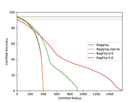
(a) $\textsc{f}_{1}$ on MNIST

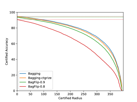
(b) $\textsc{f}_{\infty}$ on MNIST

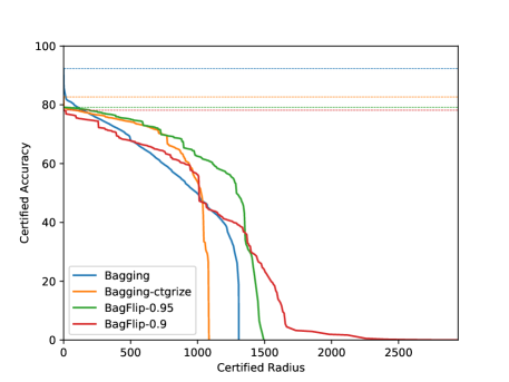
(c) $\textsc{f}_{1}$ on EMBER

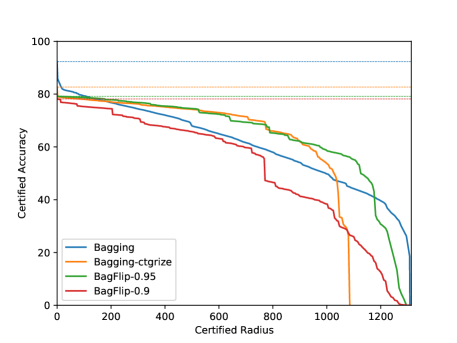
(d) $\textsc{f}_{\infty}$ on EMBER

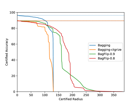
(e) $\textsc{f}_{1}$ on Contagio

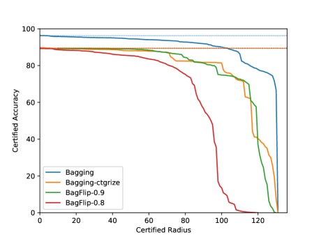
(f) $\textsc{f}_{\infty}$ on Contagio

Figure 3: Compared to Bagging [15]. The horizontal dashed lines show the normal accuracy. The solid lines show the certified accuracy at different $R$. BagFlip-$a$ shows the result of the noise level $a$. The blue line shows the uncategorized version of bagging.

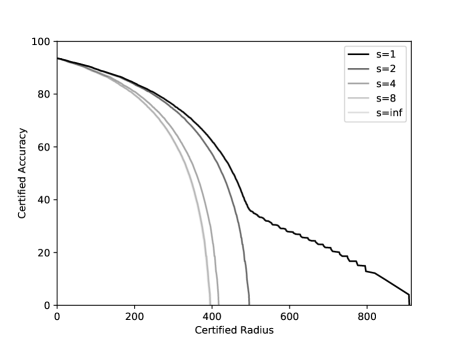
(a) BagFlip-0.9 on MNIST

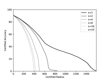
(b) BagFlip-0.8 on MNIST

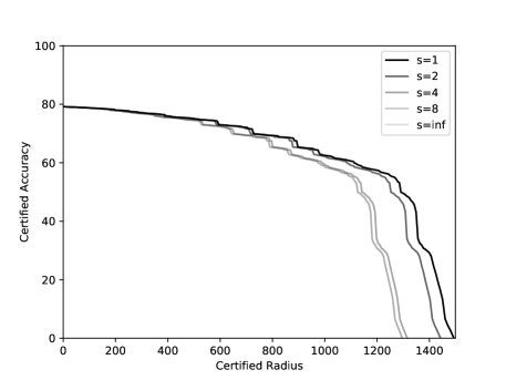
(c) BagFlip-0.95 on EMBER

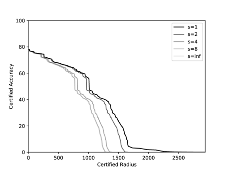
(d) BagFlip-0.9 on EMBER

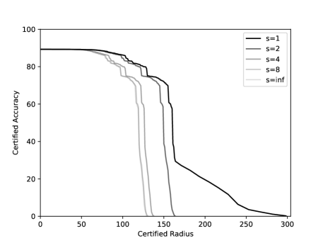
(e) BagFlip-0.9 on Contagio

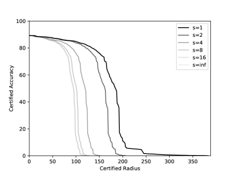
(f) BagFlip-0.8 on Contagio

Figure 4: Results of BagFlip on different $s$ and different datasets.

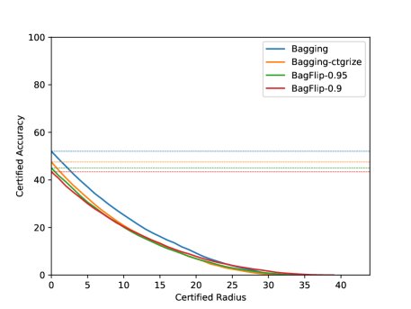
(a) $\textsc{f}_{1}$ on CIFAR10

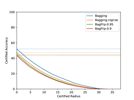
(b) $\textsc{f}_{1}$ on CIFAR10

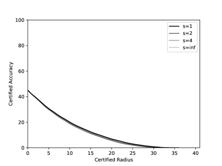
(c) BagFlip-0.95 on CIFAR10

(d) BagFlip-0.9 on CIFAR10

Figure 5: Results of BagFlip on CIFAR10.

E.2 Experiment Results Details

Table 3: This paper compared to other approaches. RAB [39] can handle perturbation $\textsc{f}_{s}^{*}$ that perturbs the input within a $l_{2}$-norm ball of radius $s$.

Approach	Perturbation $\pi$	Probability measure $\mu$	Goal
Jia et al. [15], Chen et al. [4]	Any	Bagging	Trigger-less
Rosenfeld et al. [28]	l	Noise	Trigger-less
RAB [39]	$\textsc{f}_{s}^{*}$	Noise	Trigger-less, Backdoor
Wang et al. [35]	$\textsc{fl}_{s},\textsc{f}_{s},\textsc{l}$	Noise	Trigger-less, Backdoor
This paper	$\textsc{fl}_{s},\textsc{f}_{s},\textsc{l}$	Bagging+Noise	Trigger-less, Backdoor

We train all models on a server running Ubuntu 18.04.5 LTS with two V100 32GB GPUs and Intel Xeon Gold 5115 CPUs running at 2.40GHz. For computing the certified radius, we run experiments across hundreds of machines in high throughput computing center.

E.2.1 Defend Trigger-less Attacks

Comparison to Bagging

We show full results of comparison on $\textsc{f}_{s}$ in Figures 3 4 and 5. The results are similar as described in Section 7.

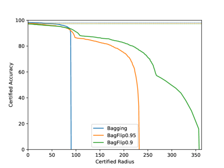
(a) Compared to Bagging on $\textsc{fl}_{1}$ on MNIST-17

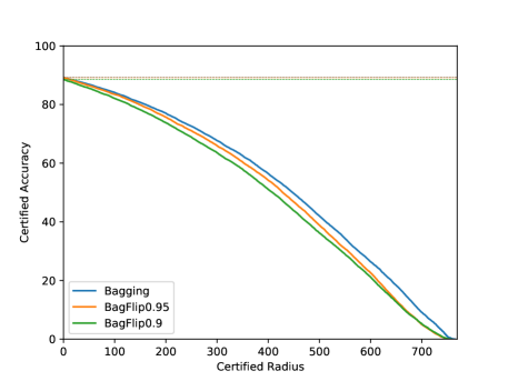
(b) Compared to Bagging on l using MNIST

Figure 6: Compared to Bagging on $\textsc{fl}_{1}$ on MNIST-17 and l using MNIST.

We additionally compare BagFlip with Bagging on $\textsc{fl}_{1}$ using MNIST-17 and l using MNIST, and show the results in Figure 6. BagFlip still outperforms Bagging on $\textsc{fl}_{1}$ using MNIST-17. However, Bagging outperforms BagFlip on l because when the attacker is only able to perturb the label, then $s=1$ is equal to $s=\infty$ and flipping the labels hurts the accuracy.

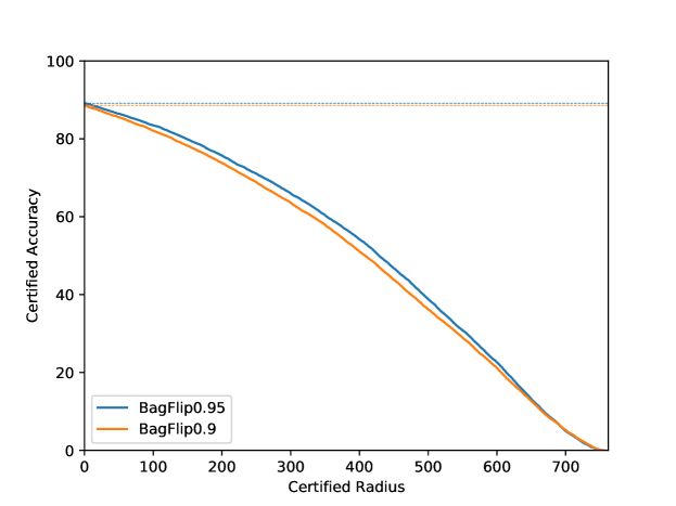
Figure 7: Results of BagFlip on l.

Comparison to LabelFlip

We compare two configurations of BagFlip to LabelFlip using MNIST and show results of BagFlip in Figure 7. The results show that LabelFlip achieves less than $60\%$ normal accuracy, while BagFlip-0.95 (BagFlip-0.9) achieves 89.2% (88.6%) normal accuracy, respectively. BagFlip achieves higher certified accuracy than LabelFlip across all $R$. In particular, the certified accuracy of LabelFlip drops to less than $20\%$ when $R=0.83$, while BagFlip-0.95 (BagFlip-0.9) still achieves 38.9% (36.2%) certified accuracy, respectively. BagFlip has higher normal accuracy and certified accuracy than LabelFlip.

E.2.2 Defend Backdoor Attacks

We set $k=100$ for MNIST-17 when comparing to FeatFlip. We set $k=50,200$ for MNIST-01 and CIFAR10-02 respectively when comparing to RAB. And we set $k=100,1000,3000,30$ for MNIST, CIFAR10, EMBER, and Contagio respectively when evaluating BagFlip on $\textsc{f}_{1}$. We use BadNets to modify 10% of examples in the training set.

Comparison to RAB

We show the comparison with full configurations of RAB-$\sigma$ in Figures 8(a) and 8(b), where $\sigma=0.5,1,2$ are different Gaussian noise levels. Note that RAB’s curves are not visible because the certified radius is almost zero anywhere.

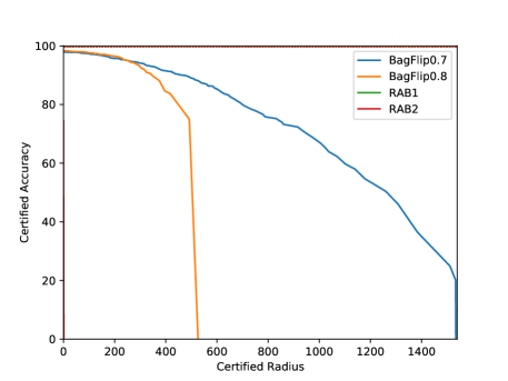
(a) Compared to RAB on MNIST-01

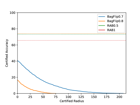
(b) Compared to RAB on CIFAR10-02

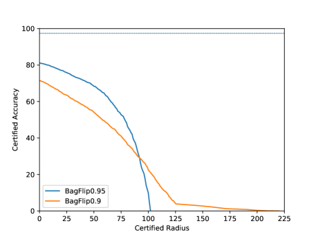
(c) Compared to FeatFlip on MNIST-17

Figure 8: Compared to FeatFlip and RAB.

Figure 9: BagFlip-0.95 on EMBER against backdoor attack with $\textsc{f}_{1}$. Dashed lines show normal accuracy.

Results on EMBER and CIFAR10

BagFlip cannot compute effective certificates for CIFAR10, i.e., the certified accuracy is zero even at $R=0$, thus we do not show the figure for CIFAR10. Figure 9 shows the results of BagFlip on EMBER. BagFlip cannot compute effective certificates for EMBER, neither. We leave the improvement of BagFlip as a future work.

References

- Aghakhani et al. [2021] Hojjat Aghakhani, Dongyu Meng, Yu-Xiang Wang, Christopher Kruegel, and Giovanni Vigna. Bullseye polytope: A scalable clean-label poisoning attack with improved transferability. In IEEE European Symposium on Security and Privacy, EuroS&P 2021, Vienna, Austria, September 6-10, 2021, pages 159–178. IEEE, 2021. doi: 10.1109/EuroSP51992.2021.00021. URL https://doi.org/10.1109/EuroSP51992.2021.00021.
- Anderson and Roth [2018] Hyrum S. Anderson and Phil Roth. EMBER: an open dataset for training static PE malware machine learning models. CoRR, abs/1804.04637, 2018. URL http://arxiv.org/abs/1804.04637.
- Biggio et al. [2012] Battista Biggio, Blaine Nelson, and Pavel Laskov. Poisoning attacks against support vector machines. In Proceedings of the 29th International Conference on Machine Learning, ICML 2012, Edinburgh, Scotland, UK, June 26 - July 1, 2012. icml.cc / Omnipress, 2012. URL http://icml.cc/2012/papers/880.pdf.
- Chen et al. [2020] Ruoxin Chen, Jie Li, Chentao Wu, Bin Sheng, and Ping Li. A framework of randomized selection based certified defenses against data poisoning attacks. CoRR, abs/2009.08739, 2020. URL https://arxiv.org/abs/2009.08739.
- Chen et al. [2017] Xinyun Chen, Chang Liu, Bo Li, Kimberly Lu, and Dawn Song. Targeted backdoor attacks on deep learning systems using data poisoning. CoRR, abs/1712.05526, 2017. URL http://arxiv.org/abs/1712.05526.
- Cohen et al. [2019] Jeremy M. Cohen, Elan Rosenfeld, and J. Zico Kolter. Certified adversarial robustness via randomized smoothing. In Kamalika Chaudhuri and Ruslan Salakhutdinov, editors, Proceedings of the 36th International Conference on Machine Learning, ICML 2019, 9-15 June 2019, Long Beach, California, USA, volume 97 of Proceedings of Machine Learning Research, pages 1310–1320. PMLR, 2019. URL http://proceedings.mlr.press/v97/cohen19c.html.
- Drews et al. [2020] Samuel Drews, Aws Albarghouthi, and Loris D’Antoni. Proving data-poisoning robustness in decision trees. In Alastair F. Donaldson and Emina Torlak, editors, Proceedings of the 41st ACM SIGPLAN International Conference on Programming Language Design and Implementation, PLDI 2020, London, UK, June 15-20, 2020, pages 1083–1097. ACM, 2020. doi: 10.1145/3385412.3385975. URL https://doi.org/10.1145/3385412.3385975.
- Dvijotham et al. [2020] Krishnamurthy (Dj) Dvijotham, Jamie Hayes, Borja Balle, J. Zico Kolter, Chongli Qin, András György, Kai Xiao, Sven Gowal, and Pushmeet Kohli. A framework for robustness certification of smoothed classifiers using f-divergences. In 8th International Conference on Learning Representations, ICLR 2020, Addis Ababa, Ethiopia, April 26-30, 2020. OpenReview.net, 2020. URL https://openreview.net/forum?id=SJlKrkSFPH.
- Gao et al. [2019] Yansong Gao, Change Xu, Derui Wang, Shiping Chen, Damith Chinthana Ranasinghe, and Surya Nepal. STRIP: a defence against trojan attacks on deep neural networks. In David Balenson, editor, Proceedings of the 35th Annual Computer Security Applications Conference, ACSAC 2019, San Juan, PR, USA, December 09-13, 2019, pages 113–125. ACM, 2019. doi: 10.1145/3359789.3359790. URL https://doi.org/10.1145/3359789.3359790.
- Geiping et al. [2021a] Jonas Geiping, Liam Fowl, Gowthami Somepalli, Micah Goldblum, Michael Moeller, and Tom Goldstein. What doesn’t kill you makes you robust(er): Adversarial training against poisons and backdoors. CoRR, abs/2102.13624, 2021a. URL https://arxiv.org/abs/2102.13624.
- Geiping et al. [2021b] Jonas Geiping, Liam H. Fowl, W. Ronny Huang, Wojciech Czaja, Gavin Taylor, Michael Moeller, and Tom Goldstein. Witches’ brew: Industrial scale data poisoning via gradient matching. In 9th International Conference on Learning Representations, ICLR 2021, Virtual Event, Austria, May 3-7, 2021. OpenReview.net, 2021b. URL https://openreview.net/forum?id=01olnfLIbD.
- Gu et al. [2017] Tianyu Gu, Brendan Dolan-Gavitt, and Siddharth Garg. Badnets: Identifying vulnerabilities in the machine learning model supply chain. CoRR, abs/1708.06733, 2017. URL http://arxiv.org/abs/1708.06733.
- Hayase et al. [2021] Jonathan Hayase, Weihao Kong, Raghav Somani, and Sewoong Oh. Defense against backdoor attacks via robust covariance estimation. In Marina Meila and Tong Zhang, editors, Proceedings of the 38th International Conference on Machine Learning, ICML 2021, 18-24 July 2021, Virtual Event, volume 139 of Proceedings of Machine Learning Research, pages 4129–4139. PMLR, 2021. URL http://proceedings.mlr.press/v139/hayase21a.html.
- Jia et al. [2020] Jinyuan Jia, Xiaoyu Cao, and Neil Zhenqiang Gong. Certified robustness of nearest neighbors against data poisoning attacks. CoRR, abs/2012.03765, 2020. URL https://arxiv.org/abs/2012.03765.
- Jia et al. [2021] Jinyuan Jia, Xiaoyu Cao, and Neil Zhenqiang Gong. Intrinsic certified robustness of bagging against data poisoning attacks. In Thirty-Fifth AAAI Conference on Artificial Intelligence, AAAI 2021, Thirty-Third Conference on Innovative Applications of Artificial Intelligence, IAAI 2021, The Eleventh Symposium on Educational Advances in Artificial Intelligence, EAAI 2021, Virtual Event, February 2-9, 2021, pages 7961–7969. AAAI Press, 2021. URL https://ojs.aaai.org/index.php/AAAI/article/view/16971.
- Koh et al. [2022] Pang Wei Koh, Jacob Steinhardt, and Percy Liang. Stronger data poisoning attacks break data sanitization defenses. Mach. Learn., 111(1):1–47, 2022. doi: 10.1007/s10994-021-06119-y. URL https://doi.org/10.1007/s10994-021-06119-y.
- Kumar et al. [2020] Aounon Kumar, Alexander Levine, Tom Goldstein, and Soheil Feizi. Curse of dimensionality on randomized smoothing for certifiable robustness. In Proceedings of the 37th International Conference on Machine Learning, ICML 2020, 13-18 July 2020, Virtual Event, volume 119 of Proceedings of Machine Learning Research, pages 5458–5467. PMLR, 2020. URL http://proceedings.mlr.press/v119/kumar20b.html.
- Lee et al. [2019] Guang-He Lee, Yang Yuan, Shiyu Chang, and Tommi S. Jaakkola. Tight certificates of adversarial robustness for randomly smoothed classifiers. In Hanna M. Wallach, Hugo Larochelle, Alina Beygelzimer, Florence d’Alché-Buc, Emily B. Fox, and Roman Garnett, editors, Advances in Neural Information Processing Systems 32: Annual Conference on Neural Information Processing Systems 2019, NeurIPS 2019, December 8-14, 2019, Vancouver, BC, Canada, pages 4911–4922, 2019. URL https://proceedings.neurips.cc/paper/2019/hash/fa2e8c4385712f9a1d24c363a2cbe5b8-Abstract.html.
- Levine and Feizi [2021] Alexander Levine and Soheil Feizi. Deep partition aggregation: Provable defenses against general poisoning attacks. In 9th International Conference on Learning Representations, ICLR 2021, Virtual Event, Austria, May 3-7, 2021. OpenReview.net, 2021. URL https://openreview.net/forum?id=YUGG2tFuPM.
- Liu et al. [2018a] Kang Liu, Brendan Dolan-Gavitt, and Siddharth Garg. Fine-pruning: Defending against backdooring attacks on deep neural networks. In Michael Bailey, Thorsten Holz, Manolis Stamatogiannakis, and Sotiris Ioannidis, editors, Research in Attacks, Intrusions, and Defenses - 21st International Symposium, RAID 2018, Heraklion, Crete, Greece, September 10-12, 2018, Proceedings, volume 11050 of Lecture Notes in Computer Science, pages 273–294. Springer, 2018a. doi: 10.1007/978-3-030-00470-5\_13. URL https://doi.org/10.1007/978-3-030-00470-5_13.
- Liu et al. [2018b] Yingqi Liu, Shiqing Ma, Yousra Aafer, Wen-Chuan Lee, Juan Zhai, Weihang Wang, and Xiangyu Zhang. Trojaning attack on neural networks. In 25th Annual Network and Distributed System Security Symposium, NDSS 2018, San Diego, California, USA, February 18-21, 2018. The Internet Society, 2018b. URL http://wp.internetsociety.org/ndss/wp-content/uploads/sites/25/2018/02/ndss2018_03A-5_Liu_paper.pdf.
- Ma et al. [2019] Yuzhe Ma, Xiaojin Zhu, and Justin Hsu. Data poisoning against differentially-private learners: Attacks and defenses. In Sarit Kraus, editor, Proceedings of the Twenty-Eighth International Joint Conference on Artificial Intelligence, IJCAI 2019, Macao, China, August 10-16, 2019, pages 4732–4738. ijcai.org, 2019. doi: 10.24963/ijcai.2019/657. URL https://doi.org/10.24963/ijcai.2019/657.
- Meyer et al. [2021] Anna P. Meyer, Aws Albarghouthi, and Loris D’Antoni. Certifying robustness to programmable data bias in decision trees. In Marc’Aurelio Ranzato, Alina Beygelzimer, Yann N. Dauphin, Percy Liang, and Jennifer Wortman Vaughan, editors, Advances in Neural Information Processing Systems 34: Annual Conference on Neural Information Processing Systems 2021, NeurIPS 2021, December 6-14, 2021, virtual, pages 26276–26288, 2021. URL https://proceedings.neurips.cc/paper/2021/hash/dcf531edc9b229acfe0f4b87e1e278dd-Abstract.html.
- Nelson et al. [2008] Blaine Nelson, Marco Barreno, Fuching Jack Chi, Anthony D. Joseph, Benjamin I. P. Rubinstein, Udam Saini, Charles Sutton, J. Doug Tygar, and Kai Xia. Exploiting machine learning to subvert your spam filter. In Fabian Monrose, editor, First USENIX Workshop on Large-Scale Exploits and Emergent Threats, LEET ’08, San Francisco, CA, USA, April 15, 2008, Proceedings. USENIX Association, 2008. URL http://www.usenix.org/events/leet08/tech/full_papers/nelson/nelson.pdf.
- Qi et al. [2021] Fanchao Qi, Yuan Yao, Sophia Xu, Zhiyuan Liu, and Maosong Sun. Turn the combination lock: Learnable textual backdoor attacks via word substitution. In Chengqing Zong, Fei Xia, Wenjie Li, and Roberto Navigli, editors, Proceedings of the 59th Annual Meeting of the Association for Computational Linguistics and the 11th International Joint Conference on Natural Language Processing, ACL/IJCNLP 2021, (Volume 1: Long Papers), Virtual Event, August 1-6, 2021, pages 4873–4883. Association for Computational Linguistics, 2021. doi: 10.18653/v1/2021.acl-long.377. URL https://doi.org/10.18653/v1/2021.acl-long.377.
- Qiao et al. [2019] Ximing Qiao, Yukun Yang, and Hai Li. Defending neural backdoors via generative distribution modeling. In Hanna M. Wallach, Hugo Larochelle, Alina Beygelzimer, Florence d’Alché-Buc, Emily B. Fox, and Roman Garnett, editors, Advances in Neural Information Processing Systems 32: Annual Conference on Neural Information Processing Systems 2019, NeurIPS 2019, December 8-14, 2019, Vancouver, BC, Canada, pages 14004–14013, 2019. URL https://proceedings.neurips.cc/paper/2019/hash/78211247db84d96acf4e00092a7fba80-Abstract.html.
- Ramakrishnan and Albarghouthi [2020] Goutham Ramakrishnan and Aws Albarghouthi. Backdoors in neural models of source code. CoRR, abs/2006.06841, 2020. URL https://arxiv.org/abs/2006.06841.
- Rosenfeld et al. [2020] Elan Rosenfeld, Ezra Winston, Pradeep Ravikumar, and J. Zico Kolter. Certified robustness to label-flipping attacks via randomized smoothing. In Proceedings of the 37th International Conference on Machine Learning, ICML 2020, 13-18 July 2020, Virtual Event, volume 119 of Proceedings of Machine Learning Research, pages 8230–8241. PMLR, 2020. URL http://proceedings.mlr.press/v119/rosenfeld20b.html.
- Saha et al. [2020] Aniruddha Saha, Akshayvarun Subramanya, and Hamed Pirsiavash. Hidden trigger backdoor attacks. In The Thirty-Fourth AAAI Conference on Artificial Intelligence, AAAI 2020, The Thirty-Second Innovative Applications of Artificial Intelligence Conference, IAAI 2020, The Tenth AAAI Symposium on Educational Advances in Artificial Intelligence, EAAI 2020, New York, NY, USA, February 7-12, 2020, pages 11957–11965. AAAI Press, 2020. URL https://ojs.aaai.org/index.php/AAAI/article/view/6871.
- Severi et al. [2021] Giorgio Severi, Jim Meyer, Scott E. Coull, and Alina Oprea. Explanation-guided backdoor poisoning attacks against malware classifiers. In Michael Bailey and Rachel Greenstadt, editors, 30th USENIX Security Symposium, USENIX Security 2021, August 11-13, 2021, pages 1487–1504. USENIX Association, 2021. URL https://www.usenix.org/conference/usenixsecurity21/presentation/severi.
- Shafahi et al. [2018] Ali Shafahi, W. Ronny Huang, Mahyar Najibi, Octavian Suciu, Christoph Studer, Tudor Dumitras, and Tom Goldstein. Poison frogs! targeted clean-label poisoning attacks on neural networks. In Samy Bengio, Hanna M. Wallach, Hugo Larochelle, Kristen Grauman, Nicolò Cesa-Bianchi, and Roman Garnett, editors, Advances in Neural Information Processing Systems 31: Annual Conference on Neural Information Processing Systems 2018, NeurIPS 2018, December 3-8, 2018, Montréal, Canada, pages 6106–6116, 2018. URL https://proceedings.neurips.cc/paper/2018/hash/22722a343513ed45f14905eb07621686-Abstract.html.
- Tramèr et al. [2020] Florian Tramèr, Nicholas Carlini, Wieland Brendel, and Aleksander Madry. On adaptive attacks to adversarial example defenses. In Hugo Larochelle, Marc’Aurelio Ranzato, Raia Hadsell, Maria-Florina Balcan, and Hsuan-Tien Lin, editors, Advances in Neural Information Processing Systems 33: Annual Conference on Neural Information Processing Systems 2020, NeurIPS 2020, December 6-12, 2020, virtual, 2020. URL https://proceedings.neurips.cc/paper/2020/hash/11f38f8ecd71867b42433548d1078e38-Abstract.html.
- Tran et al. [2018] Brandon Tran, Jerry Li, and Aleksander Madry. Spectral signatures in backdoor attacks. In Samy Bengio, Hanna M. Wallach, Hugo Larochelle, Kristen Grauman, Nicolò Cesa-Bianchi, and Roman Garnett, editors, Advances in Neural Information Processing Systems 31: Annual Conference on Neural Information Processing Systems 2018, NeurIPS 2018, December 3-8, 2018, Montréal, Canada, pages 8011–8021, 2018. URL https://proceedings.neurips.cc/paper/2018/hash/280cf18baf4311c92aa5a042336587d3-Abstract.html.
- Turner et al. [2019] Alexander Turner, Dimitris Tsipras, and Aleksander Madry. Label-consistent backdoor attacks. CoRR, abs/1912.02771, 2019. URL http://arxiv.org/abs/1912.02771.
- Wang et al. [2020a] Binghui Wang, Xiaoyu Cao, Jinyuan Jia, and Neil Zhenqiang Gong. On certifying robustness against backdoor attacks via randomized smoothing. CoRR, abs/2002.11750, 2020a. URL https://arxiv.org/abs/2002.11750.
- Wang et al. [2019] Bolun Wang, Yuanshun Yao, Shawn Shan, Huiying Li, Bimal Viswanath, Haitao Zheng, and Ben Y. Zhao. Neural cleanse: Identifying and mitigating backdoor attacks in neural networks. In 2019 IEEE Symposium on Security and Privacy, SP 2019, San Francisco, CA, USA, May 19-23, 2019, pages 707–723. IEEE, 2019. doi: 10.1109/SP.2019.00031. URL https://doi.org/10.1109/SP.2019.00031.
- Wang et al. [2020b] Hongyi Wang, Kartik Sreenivasan, Shashank Rajput, Harit Vishwakarma, Saurabh Agarwal, Jy-yong Sohn, Kangwook Lee, and Dimitris S. Papailiopoulos. Attack of the tails: Yes, you really can backdoor federated learning. In Hugo Larochelle, Marc’Aurelio Ranzato, Raia Hadsell, Maria-Florina Balcan, and Hsuan-Tien Lin, editors, Advances in Neural Information Processing Systems 33: Annual Conference on Neural Information Processing Systems 2020, NeurIPS 2020, December 6-12, 2020, virtual, 2020b. URL https://proceedings.neurips.cc/paper/2020/hash/b8ffa41d4e492f0fad2f13e29e1762eb-Abstract.html.
- Wang et al. [2022] Wenxiao Wang, Alexander Levine, and Soheil Feizi. Improved certified defenses against data poisoning with (deterministic) finite aggregation. CoRR, abs/2202.02628, 2022. URL https://arxiv.org/abs/2202.02628.
- Weber et al. [2020] Maurice Weber, Xiaojun Xu, Bojan Karlas, Ce Zhang, and Bo Li. RAB: provable robustness against backdoor attacks. CoRR, abs/2003.08904, 2020. URL https://arxiv.org/abs/2003.08904.
- Xiao et al. [2015] Huang Xiao, Battista Biggio, Gavin Brown, Giorgio Fumera, Claudia Eckert, and Fabio Roli. Is feature selection secure against training data poisoning? In Francis R. Bach and David M. Blei, editors, Proceedings of the 32nd International Conference on Machine Learning, ICML 2015, Lille, France, 6-11 July 2015, volume 37 of JMLR Workshop and Conference Proceedings, pages 1689–1698. JMLR.org, 2015. URL http://proceedings.mlr.press/v37/xiao15.html.
- Yao et al. [2019] Yuanshun Yao, Huiying Li, Haitao Zheng, and Ben Y. Zhao. Latent backdoor attacks on deep neural networks. In Lorenzo Cavallaro, Johannes Kinder, XiaoFeng Wang, and Jonathan Katz, editors, Proceedings of the 2019 ACM SIGSAC Conference on Computer and Communications Security, CCS 2019, London, UK, November 11-15, 2019, pages 2041–2055. ACM, 2019. doi: 10.1145/3319535.3354209. URL https://doi.org/10.1145/3319535.3354209.
- Zhu et al. [2019] Chen Zhu, W. Ronny Huang, Hengduo Li, Gavin Taylor, Christoph Studer, and Tom Goldstein. Transferable clean-label poisoning attacks on deep neural nets. In Kamalika Chaudhuri and Ruslan Salakhutdinov, editors, Proceedings of the 36th International Conference on Machine Learning, ICML 2019, 9-15 June 2019, Long Beach, California, USA, volume 97 of Proceedings of Machine Learning Research, pages 7614–7623. PMLR, 2019. URL http://proceedings.mlr.press/v97/zhu19a.html.