Geometry of transcendental singularities of complex analytic functions and vector fields

Abstract.

We study transcendental meromorphic functions with essential singularities on Riemann surfaces. Every function $\Psi_{X}$ has associated a complex vector field $X$. In the converse direction, vector fields $X$ provide single valued or multivalued functions $\Psi_{X}$. Our goal is to understand the relationship between the analytical properties of $\Psi_{X}$, the singularities of its inverse $\Psi_{X}^{-1}$ and the geometric behavior of $X$. As first result, by examining the containment properties of the neighborhoods of the singularities of $\Psi_{X}^{-1}$, we characterize when a singularity of $\Psi_{X}^{-1}$ over a singular value $a$, is either algebraic, logarithmic or non logarithmic. Secondly, to make precise the cooperative aspects between analysis and geometry, we present the systematic study of two holomorphic families of transcendental functions with an essential singularity at infinity, as well as some sporadic examples. As third stage, we study the incompleteness of the trajectories of the associated vector field $X$ with essential singularities on a Riemann surface $M_{\mathfrak{g}}$ of genus ${\mathfrak{g}}$. As an application, we provide conditions under which there exists an infinite number of (real) incomplete trajectories of $X$ localized at the essential singularities. Furthermore, removing the incomplete trajectories decomposes the Riemann surface into real flow invariant canonical pieces.

Alvaro Alvarez–Parrilla^∗

Grupo Alximia SA de CV

Ensenada, Baja California, CP 22800, México

Jesús Muciño–Raymundo

Centro de Ciencias Matemáticas

Universidad Nacional Autónoma de México, Morelia, México

1. Introduction

Essential singularities for meromorphic functions on the Riemann sphere are a natural source of intricate/complex behavior in analysis, iteration of functions and differential equations, among others topics. The analytic description of essential singularities is a mature research subject. Our naive goal is to describe the geometric aspects of (non necessarily isolated) essential singularities.

We consider $\Psi_{X}:M\longrightarrow{\widehat{\mathbb{C}}}_{t}$ a transcendental meromorphic function on an arbitrary Riemann surface $M$, that is with an essential singularity at $e\in M$. In order to study the geometry of the essential singularity, we shall consider the singularities of $\Psi_{X}^{-1}$, via the associated vector field $X$. In fact, our main tool is to recognize that there exists a singular complex analytic vector field $X$ on $M$ canonically associated to $\Psi_{X}$. Conversely, given $X$ a complex analytic vector field, the associated $\Psi_{X}$ is single valued when the 1–form of time of $X$ has zero residues and periods. See §2, in particular Definition 2.1 for singular complex analytic notion, and Diagram 5 for the correspondence.

The classical analytic classification of the singularities of $\Psi_{X}^{-1}$ is as follows

a) algebraic singularities, arising from the critical values of $\Psi_{X}$, and

b) transcendental singularities, originating from the asymptotic values of $\Psi_{X}$.

In the vector field framework, cases (a) and (b) correspond to

A) poles and zeros of $X$, and

B) essential singularities of $X$, respectively.

Furthermore, due to F. Iversen [24], transcendental singularities of $\Psi_{X}^{-1}$ in turn subdivide into

b.i) direct logarithmic singularities,

b.ii) direct non logarithmic singularities, and

b.iii) indirect singularities.

We shall use “non logarithmic” without the “direct” adjective when referring to direct non logarithmic as well as indirect singularities. See §3.

In order to better understand the singularities of $\Psi_{X}^{-1}$ over the singular values $\{a\}\subset{\widehat{\mathbb{C}}}_{t}$ of $\Psi$, it is usual to add some ideal points $U_{a}$ to $M$, defining neighborhoods $U_{a}(\rho)\subset M$ of theses points, see Definition 3.1.

The usefulness of vector fields $X$ in the study of functions $\Psi_{X}$ can be roughly stated as follows. The vector field distinguishes the finite and infinite asymptotic values $a\in{\widehat{\mathbb{C}}}_{t}$ of $\Psi_{X}$ and its ideal points $U_{a}$, in a clear geometric way. A natural/heuristic idea of this is to exploit the phase portrait of $X$. Even though we can not directly observe the asymptotic values of $\Psi_{X}$, it is possible to identify the ideal points $U_{a}$ of $\Psi_{X}^{-1}$. Moreover, each vector field originates a singular flat metric in its domain, so that the real trajectories of the vector field are geodesics. The incomplete real trajectories of $X$ (other than those arriving or exiting poles) coincide with the asymptotic trajectories of $\Psi_{X}$.

In previous works, we have exploited some of these ideas, see [31], [2] and [4].

Regarding the singularities of $\Psi_{X}^{-1}$, the cases of algebraic and direct logarithmic singularities are understood best; in particular, the following classical theorem was well known to R. Nevanlinna, see [33] Ch. XI, §1.3.

A transcendental singularity of $\Psi^{-1}$ over an isolated asymptotic value is logarithmic.

We shall prove a stronger version of the above theorem. To do this, we first introduce the notion of separable applied to two singularities $U_{a}$ and $U_{b}$ of $\Psi^{-1}_{X}$ over the singular values $a$ and $b$, respectively. Roughly speaking, $U_{a}$ and $U_{b}$ are separable if their neighborhoods in ${\widehat{\mathbb{C}}}_{z}$, are disjoint for small enough radii, see Definition 3.12 for full details. Furthermore, a singularity $U_{a}$ is separate if given any other singularity $U_{b}$, $U_{a}$ and $U_{b}$ are separable. A source of difficulties is that $a$ and $b$ can be the same singular value and yet $U_{a}$ and $U_{b}$ can be different singularities of $\Psi^{-1}_{X}$. See Examples 4.4–4.8 in §4. The above concepts provide topological simplicity for logarithmic singularities.

Theorem 1.1.

Let $\Psi_{X}:M\longrightarrow{\widehat{\mathbb{C}}}_{t}$ be a transcendental meromorphic function with an essential singularity at $e\in M$. A singularity $U_{a}$ of $\Psi_{X}^{-1}$ is separate if and only if $U_{a}$ is algebraic or logarithmic.

From the vector field perspective, a priori, the relation between (B) and (b.i–iii) is unknown. The use of the phase portrait of $X$ allows us to, for instance, describe the logarithmic singularities of $\Psi^{-1}_{X}$ in geometric terms. The exponential tracts of $\Psi$ can be naturally classified as elliptic and hyperbolic, see Figures 3, 4 and 5.

The cooperative aspects of our methods for functions and vector fields allows us to study finite dimensional holomorphic families and sporadic examples of essential singularities. Section 4 presents two subfamilies in the Speiser class. The first family is composed of functions of type

$$\Psi_{X}(z)=\int^{z}P(\zeta){\text{\myfont e}}^{-E(\zeta)}d\zeta,$$

with $P(z),\,E(z)$ polynomials of degrees $r$ and $d\geq 1$, respectively; see Theorem 4.2 and our previous work [4]. The second family is given by functions of type

$$\Psi_{X}(z)=R\circ{\text{\myfont e}}^{2\pi iz/T},$$

where $R(w)$ are rational functions of degree ${\tt r}\geq 1$, $T\in{\mathbb{C}}^{*}$. A systematic description that depends on the behavior of $R$ is provided in Theorem 4.3. Note that this family is the simplest having periodic functions and/or vector fields, where accumulation of zeros and poles at the essential singularity $\infty$ appears. Furthermore, in §4.3, a necessarily small collection of sporadic examples is provided. These families and examples illustrate the links between analysis and geometry.

We recall that a complete holomorphic vector field on a complex manifold has complex flow for all complex time and all initial conditions. Complete vector fields describe the one–parameter families of biholomorphisms of complex manifolds, see [27] Ch. III, [13] Ch. 4. On ${\mathbb{C}}^{n}$, complete entire vector fields are among the more interesting families of complex differential equations. On Riemann surfaces complete vector fields are rare. An incomplete trajectory of a complex analytic vector field $X$ is a real trajectory of it having as maximal domain of existence a strict subset of ${\mathbb{R}}$. In [16], A. Guillot explores some relations between complex differential equations and the geometrical properties of their complex trajectories, looking at interesting incomplete (real) trajectories. In §5, vector field tools provide us with the following result

Theorem 1.2.

Every non rational, singular complex analytic vector field $X$ on a compact Riemann surface $M_{\mathfrak{g}}$, of genus $\mathfrak{g}$, has an infinite number of incomplete trajectories.

This raises a natural question. Which neighborhoods $U_{a}(\rho)$ of the singularities of $\Psi_{X}^{-1}$ contain incomplete trajectories and how many are there? See the recent work of J. K. Langley [28]. As an application of Theorem 1.1, we prove a constructive description of how the incomplete trajectories of $X$ on an arbitrary Riemann surface $M$ arise in a vicinity of an essential singularity $e\in M$. Our result is the following.

Theorem 1.3 (Finite asymptotic values and incomplete trajectories).

Let $X$ be a singular complex analytic vector field on $M$ with an essential singularity at $e\in M$.

1. Any neighborhood $U_{a}(\rho)$ of a transcendental singularity $U_{a}$ of $\Psi_{X}^{-1}$ over a finite asymptotic value $a\in{\mathbb{C}}_{t}$, contains an infinite number of incomplete trajectories of $X$.

2. If $\Psi_{X}$ has no finite asymptotic values, then $X$ has an infinite number of poles accumulating at $e\in M$.

In addition, some comments on the singularities of $\Psi_{X}^{-1}$ for multivalued $\Psi_{X}$ are provided in §5.2. Two illustrative examples of vector fields $X$ with multivalued $\Psi_{X}$ are also given.

In §6, given a singular complex analytic vector field $X$ with a finite number of essential singularities on a compact Riemann surface $M_{\mathfrak{g}}$ of genus $\mathfrak{g}\geq 0$, we provide a decomposition of $M_{\mathfrak{g}}$ in invariant regions under the real flow, by removing the incomplete trajectories of $X$.

Finally, in §7 we suggest a new classification of transcendental singularities of $\Psi_{X}^{-1}$, based on Theorem 1.1, that provides geometrical insight into $\Psi_{X}$.

2. General facts about functions and vector fields

2.1. Functions and vector fields on Riemann surfaces

Let us recall some very general concepts.

Definition 2.1.

On any Riemann surface $M$, singular complex analytic functions, vector fields, 1–forms and quadratic differentials means that they may have accumulation of zeros, poles and/or essential singularities.

Note that the notion of singular complex analytic includes holomorphic objects on compact Riemann surfaces, which are not transcendental meromorphic. This is singular complex analytic is a larger class.

Throughout this work, we assume that the vector fields $X$ are non identically zero and the functions $\Psi$ are non identically constant.

The formal expression of a vector field $X$ in holomorphic charts $\{\phi_{\tt j}:V_{\tt j}\subset M\longrightarrow{\mathbb{C}}_{z}\}$ must be $\{f_{\tt j}(z)\frac{\partial}{\partial z}\ |\ z\in\phi_{\tt j}(V_{\tt j})\}$. Since our constructions are independent of charts on $M$, as seen in [2] §2, we avoid this cumbersome notation.

From functions to vector fields. Let

(1) $$\Psi_{X}:M\longrightarrow{\widehat{\mathbb{C}}}_{t}$$

be a singular complex analytic function. The canonical associated singular complex analytic vector field is

(2) $$X(z)=\frac{1}{\Psi_{X}^{\prime}(z)}\frac{\partial}{\partial z},\ \ \ \hbox{ on }M.$$

From vector fields to functions. Let

(3) $$X(z)=f(z)\frac{\partial}{\partial z}$$

be a singular complex analytic vector field on $M$.

Definition 2.2.

Let $X$ be as above, we shall denote by $\mathcal{Z}$ the zeros, $\mathcal{P}$ the poles, $\mathbb{E}$ the isolated essential isolated singularities and

$\mathcal{S}_{X}=\overline{(\mathcal{Z}\cup\mathcal{P}\cup\mathbb{E})}\subset M$

as the singular set of $X$, here $\overline{(\ \ )}$ denotes the closure.

The additively automorphic multivalued function associated to $X$ is

(4) $$\Psi_{X}(z)=\int^{z}\frac{d\zeta}{f(\zeta)}:(M\backslash\mathcal{S}_{X})\cup\mathcal{P}\longrightarrow{\widehat{\mathbb{C}}}_{t}$$

is a single valued function. Moreover, the associated singular complex analytic 1–form of time is $\omega_{X}=dz/f(z)$. Clearly, the poles of $X$ determine zeros of $\omega_{X}$ and critical points of $\Psi_{X}$ in $M$; the points of $\mathcal{P}$ are allowed in the domain of $\Psi_{X}$.

Remark 2.3.

Let $X$ be a singular complex analytic vector field on a Riemann surface $M$. By definition the 1–form of time $\omega_{X}$ of $X$ satisfies $\omega_{X}(X)\equiv 1$. Note that $\Psi_{X}(z)=\int^{z}\omega_{X}$, where $\omega_{X}$ is a singular complex analytic 1–form on $M$.

In order to obtain a single valued $\Psi_{X}(z)$;

i) the residues $\frac{1}{2\pi i}\int_{\gamma}{\omega_{X}}$ of the 1–form of time, and

ii) the periods $\int_{\gamma}{\omega_{X}}$, where $\gamma$ determines a non trivial class in $H_{1}(M,{\mathbb{Z}})$,

are required to be zero.

In both cases, single valued or multivalued, $\Psi_{X}$ is a global flow box that rectifies the corresponding singular complex analytic vector field $X$, thus

$\big{(}\Psi_{X}\big{)}_{*}X=\frac{\partial}{\partial t}$.

The multivalued global flow box $\Psi_{X}$ case appears in Proposition 2.4 and in §5, §6.

Proposition 2.4 (Dictionary between the singular analytic objects, [31], [2]).

On a Riemann surface $M$ there exists a canonical correspondence between the following objects.

1. A singular complex analytic vector field $X=f(z)\frac{\partial}{\partial z}$, as in (3).

2. A singular complex analytic 1–form $\omega_{X}=dz/f(z)$.

3. A singular complex analytic additively automorphic multivalued function $\Psi_{X}(z)=\int^{z}\frac{d\zeta}{f(\zeta)}$ as in (4), it is a global flow box for $X$.

4. An orientable singular complex analytic quadratic differential $\mathcal{Q}_{X}=\omega_{X}\otimes\omega_{X}$, here the trajectories of $X$ coincide with horizontal trajectories of $\mathcal{Q}_{X}$.

5. A singular flat metric $g_{X}=\Psi^{*}|dt|$, which is the pullback of the flat Riemannian metric $|dt|=d\tau^{2}+ds^{2}$, $t\doteq\tau+is\in{\mathbb{C}}$, having suitable singularities at $\mathcal{S}_{X}$ and a unitary geodesic vector field ${\mathfrak{Re}\left(X\right)}$. By abuse of notation, $(M,g_{X})$ denotes this singular non compact Riemannian manifold.

6. A Riemann surface ${\mathcal{R}}_{X}=\{(z,t)\ |\ t=\Psi_{X}(z)\}\subset M\times{\widehat{\mathbb{C}}}_{t}$ associated to a singular complex analytic function $\Psi_{X}$.

Diagrammatically,

Proof.

A detailed proof is in [2], §2. We provide here two precisions.

Let $\pi_{1}(z,t)=z$, $\pi_{2}(z,t)=t$ be the canonical projections in $M\times{\widehat{\mathbb{C}}}_{t}$. The flat metric on $\big{(}{\mathcal{R}}_{X},\pi_{2}^{*}(\frac{\partial}{\partial t})\big{)}$ is induced by the flat Riemannian metric $\big{(}{\widehat{\mathbb{C}}},|dt|\big{)}$, equivalently $\big{(}{\widehat{\mathbb{C}}}_{t},\frac{\partial}{\partial t}\big{)}$, via the projection of $\pi_{2}$.

Assertions (3) and (6) should be understood in the following sense. For two initial points $z_{0}$, $z_{1}$, where $X$ is a non zero holomorphic vector field, it follows that $\Psi_{X}(z)=\int_{z_{0}}^{z}\omega_{X}=\int_{z_{1}}^{z}\omega_{X}+c$. Hence, $\Psi_{X}$ is unique up to a constant and the corresponding Riemann surface provided with a vector field $\big{(}{\mathcal{R}}_{X},\,\pi_{2}^{*}(\frac{\partial}{\partial t})\big{)}$ is well defined, independently of the initial point $z_{0}$. ∎

Lemma 2.5.

1. The following diagram commutes

   and $\pi_{1}$ is an isometry.

2. Moreover, $\Psi_{X}$ is single valued if and only if the projection $\pi_{1}$ is a biholomorphism between

   $\big{(}{\mathcal{R}}_{X},\pi^{*}_{2}(\frac{\partial}{\partial t})\big{)}$  and   $(M,X)$.

3. The (ideal) boundary of ${\mathcal{R}}_{X}$ is totally disconnected, separable and compact.

Proof.

(1) and (2) are straightforward, see also [2] diagram 2.6 and lemma 2.7. A proof of (3) can be found in [34] as proposition 3. ∎

In what follows, unless explicitly stated, we shall use the abbreviated form ${\mathcal{R}}_{X}$ instead of the more cumbersome $\big{(}{\mathcal{R}}_{X},\pi^{*}_{2}(\frac{\partial}{\partial t})\big{)}$.

Definition 2.6.

A maximal real trajectory of $X$ is $z(\tau):(a,b)\subseteq{\mathbb{R}}\longrightarrow M$, where $a,b\in{\mathbb{R}}\cup\{\pm\infty\}$, $a<b$, satisfying that $\frac{dz(\tau)}{d\tau}=f(z(\tau))$. Equivalently, $z(\tau)$ is a trajectory of the associated real vector field ${\mathfrak{Re}\left(X\right)}$.

Classically, the inversion of the integral

$\Psi_{X}:(M\backslash\mathcal{S}_{X})\cup\mathcal{P}\longrightarrow{\mathbb{C}}_{t},\ \ \ z\longmapsto t=\int^{z}_{z_{0}}\frac{d\zeta}{f(\zeta)},$

say $\Psi_{X}^{-1}$, provides a complex trajectory solution of the vector field $X$; generically $\Psi_{X}$ is multivalued. Among other advantages, the trajectories $z(\tau)$ of the real vector field ${\mathfrak{Re}\left(X\right)}$ are the level sets

$\{{\mathfrak{Im}\left(\Psi_{X}(z(\tau))\right)}=cte.\}$,

i.e. the horizontal trajectories of the orientable quadratic differential $\mathcal{Q}_{X}$.

2.2. Local theory of vector fields

Recall the topological and analytical description of poles and zeros for germs of complex vector fields on holomorphic charts $({\mathbb{C}},z_{0})$, where $z_{0}\in M$ or ${\widehat{\mathbb{C}}}_{z}$. The usual notions of topological hyperbolic $H$, elliptic $E$ and parabolic $P$ sectors for isolated singularities of vector fields are enlarged to the complex analytic category as follows.

Definition 2.7.

[2] §5. Let $({\widehat{\mathbb{C}}},\frac{\partial}{\partial z})$ be the holomorphic vector field on the Riemann sphere with a double zero at $\infty$, and let $\overline{{\mathbb{H}}}^{2}=\{{\mathfrak{Im}\left(z\right)}\geq 0\}\cup\{\infty\}\subset{\widehat{\mathbb{C}}}$.

1. A hyperbolic sector is the vector field germ $H=\big{(}(\overline{{\mathbb{H}}}^{2},0),\frac{\partial}{\partial z})\big{)}$, Figure 1.c.

2. An elliptic sector is the vector field germ $E=\big{(}(\overline{{\mathbb{H}}}^{2},\infty),\frac{\partial}{\partial z})\big{)}$, equivalently $\big{(}(\overline{{\mathbb{H}}}^{2},0),-w^{2}\frac{\partial}{\partial w})\big{)}$ when $\{z\mapsto\frac{1}{z}=w\}$, Figure 1.a.

3. A right parabolic sector is the vector field germ

$P+=\big{(}\{0\leq{\mathfrak{Im}\left(z\right)}\leq h\}\cap\{{\mathfrak{Re}\left(z\right)}>0\},\infty),\frac{\partial}{\partial z})\big{)}$,

in addition the left parabolic sector $P-$   when ${\mathfrak{Re}\left(z\right)}<0$ is admissible, $h\in{\mathbb{R}}^{+}$ is a parameter, Figure 1.b.

4. An entire sector is the vector field germ $\mathscr{E}=\big{(}(\overline{{\mathbb{H}}}^{2},\infty),{\text{\myfont e}}^{z}\frac{\partial}{\partial z}\big{)}$, Figure 4.b.

The sectors are germs of flat Riemannian manifolds with boundary provided with a complex vector field; in [2] §5 we describe their properties. Thus, we say that $X$ has a hyperbolic, elliptic, parabolic or entire sector when ${\mathfrak{Re}\left(X\right)}$ has it.

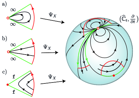
Figure 1. The hyperbolic $H$, elliptic $E$, parabolic $P$ sectors of ${\mathfrak{Re}\left(X\right)}$. The value $\infty$ is a small red circle and the finite critical value is a red point. The left drawing sketches the sphere $({\widehat{\mathbb{C}}}_{t},\frac{\partial}{\partial t})$ describing their embeddings under $\Psi_{X}$.

The following result, which is the local analytic normal form for zeros and poles of vector fields, is well known. It appears in the theory of quadratic differentials [25], [39], [1] and in complex differential equations [17], [18], [19], [8], [32], [14]. Our version stresses the interplay between the topology and the conformal properties of $X$ at the point. Hence only topological information of the real vector field ${\mathfrak{Re}\left(X\right)}$ is required in a punctured neighborhood; see Figure 2.

Proposition 2.8 (Local analytic normal forms at zeros and poles of $X$).

Let $\big{(}({\mathbb{C}},0),X\big{)}$ be a germ of a singular complex analytic vector field, in each item the corresponding assertions are equivalent.

1. i) ${\mathfrak{Re}\left(X\right)}$ is topologically equivalent to ${\mathfrak{Re}\left(\frac{\partial}{\partial t}\right)}$.

   ii) $X$ is holomorphic and non zero at $0$.

   iii) Up to local biholomorphism $X$ is $\frac{\partial}{\partial z}$.

2. i) ${\mathfrak{Re}\left(X\right)}$ has a topological center, a source or sink.

   ii) $X$ has a zero of multiplicity one at $0$.

   iii) Up to local biholomorphism $X$ is $\frac{1}{\lambda}z\frac{\partial}{\partial z}$, $\lambda\in{\mathbb{C}}^{*}$.

3. i) ${\mathfrak{Re}\left(X\right)}$ admits a decomposition with $2s-2\geq 2$ elliptic sectors and parabolic sectors.

   ii) $X$ has a zero of $X$ at $0$ multiplicity of $s\geq 2$.

   iii) Up to local biholomorphism $X$ is $(\frac{1}{\lambda}z+z^{s})\frac{\partial}{\partial z}$, $\lambda\in{\mathbb{C}}$.

4. i) ${\mathfrak{Re}\left(X\right)}$ admits a decomposition with $2k+2$ hyperbolic sectors.

   ii) $X$ has a pole of multiplicity $-k\leq-1$ at $0$.

   iii) Up to local biholomorphism $X$ is $\frac{1}{z^{k}}\frac{\partial}{\partial z}$.

5. i) ${\mathfrak{Re}\left(X\right)}$ has any other topology different from (1)–(4).

   ii) $0$ is an (non necessarily isolated) essential singularity of $X$.

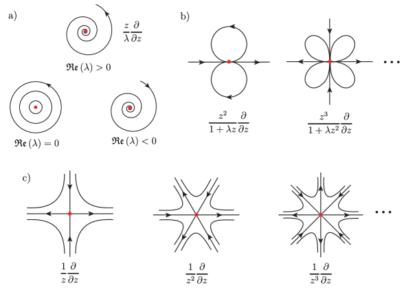
Figure 2. Local analytic normal forms; a) simple zeros, b) multiple zeros, and c) poles of $X$.

Proof.

In assertions (1)–(4), $X$ is holomorphic and non zero in a punctured disk $D(0,\rho)\backslash\{0\}$. Hence, the equivalences (1)–(4) arise from the complex analytic normal form for zeros and poles of vector fields. Moreover, in (3) the appearance of parabolic sectors is related to the residue of $\omega_{X}$, for further details see [2] §5. ∎

Table 1, describes the correspondence of local singularities for $X$, $\omega_{X}$ and $\Psi_{X}$, where $\lambda$ is the residue of $\omega_{X}$, determining the multivaluedness of $\Psi_{X}$.

Table 1. Relationship between vector fields, 1–forms and distinguished parameters.

Complex analytic	Complex analytic	Distinguished
vector field	1–form	parameter
$X(z)=f(z)\frac{\partial}{\partial z}$	$\omega_{X}(z)=\frac{dz}{f(z)}$	$\Psi_{X}(z)=\int\limits^{z}\omega_{X}$
pole of	zero of	zero of
order $-k\leq-1$	order $k$	order $k+1$
$\frac{1}{z^{k}}\frac{\partial}{\partial z}$	$z^{k}\,dz$	$\frac{1}{k+1}z^{k+1}$
simple zero	simple pole
$\frac{1}{\lambda}z\frac{\partial}{\partial z}$	$\frac{\lambda}{z}\,dz$	$\lambda\log(z)$
multiple zero $s\geq 2$	multiple pole	pole of order $s-1$ $\Leftrightarrow$ $\lambda=0$
$\frac{z^{s}}{1+\lambda z^{s-1}}\frac{\partial}{\partial z}$	$\left(\frac{1}{z^{s}}+\frac{\lambda}{z}\right)dz$	$\frac{1}{(1-s)z^{s-1}}+\lambda\log(z)$
essential	essential
singularity at $\infty$	singularity at $\infty$
${\text{\myfont e}}^{P(z)}\frac{\partial}{\partial z}$	${\text{\myfont e}}^{-P(z)}dz$	$\int\limits^{z}{\text{\myfont e}}^{-P(\zeta)}d\zeta$

3. Singularities of $\Psi^{-1}_{X}$

Let $\Psi_{X}:M_{z}\longrightarrow{\widehat{\mathbb{C}}}_{t}$ be a transcendental meromorphic function, similarly as in (1). We follow W. Bergweiler et al. [7] and A. Eremenko [10], with the obvious modifications for the case of an essential singularity of $M$. In Section 5.2, we shall extend the study to the multivalued case of $\Psi_{X}$ on $M$.

The inverse function $\Psi_{X}^{-1}$ can be defined on the Riemann surface ${\mathcal{R}}_{X}$. Since we want to study the singularities of $\Psi_{X}^{-1}$, it can be done by adding the ideal points $U_{a}$ to $M$, and defining neighborhoods $U_{a}(\rho)\subset M$ of theses points.

Let $e$ be a point in $M$ or a conformal puncture of $M$.

Definition 3.1.

Take $a\in{\widehat{\mathbb{C}}}_{t}$ and denote by $D(a,\rho)\subset{\widehat{\mathbb{C}}}_{t}$ the disk of radius $\rho>0$ (in the spherical metric) centered at $a$. For every $\rho>0$, choose a component $U_{a}(\rho)\subset M$ of $\Psi_{X}^{-1}(D(a,\rho))$ in such a way that $\rho_{1}<\rho_{2}$ implies $U_{a}(\rho_{1})\subset U_{a}(\rho_{2})$. Note that the function $U_{a}:\rho\to U_{a}(\rho)$ is completely determined by its germ at 0.

The two possibilities below can occur for the germ of $U_{a}$.

1. $\cap_{\rho>0}U_{a}(\rho)=\{z_{0}\},\,z_{0}\in{\mathbb{C}}_{z}$. In this case, $a=\Psi_{X}(z_{0})$.

   Moreover, if $a\in{\mathbb{C}}_{t}$ and $\Psi_{X}^{\prime}(z_{0})\neq 0$, or $a=\infty$ and $z_{0}$ is a simple pole of $\Psi$, then $z_{0}$ is called an ordinary point.

   On the other hand, if $a\in{\mathbb{C}}_{t}$ and $\Psi_{X}^{\prime}(z_{0})=0$, or if $a=\infty$ and $z_{0}$ is a multiple pole of $\Psi_{X}$, then $z_{0}$ is called a critical point and $a$ is called a critical value. We also say that the critical point $z_{0}$ lies over $a$. In this case, $U_{a}:\rho\to U_{a}(\rho)$ defines an algebraic singularity of $\Psi_{X}^{-1}$.

2. $\cap_{\rho>0}U_{a}(\rho)=\varnothing$. we then say that our choice $\rho\to U_{a}(\rho)$ defines a transcendental singularity of $\Psi^{-1}_{X}$, and that the transcendental singularity $U_{a}$ lies over $a$.
   For every $\rho>0$, the open set $U_{a}(\rho)\subset{\mathbb{C}}_{z}$ is called a neighborhood of the transcendental singularity $U_{a}$. So if $z_{k}\in{\mathbb{C}}_{z}$, we say that $z_{k}\to U_{a}$ if for every $\rho>0$ there exists $k_{0}$ such that $z_{k}\in U_{a}(\rho)$ for $k\geq k_{0}$.

In particular, if $M={\mathbb{C}}_{z}$ then it follows that every neighborhood $U_{a}(\rho)$ of a transcendental singularity $U_{a}$ is unbounded.

Recalling [10] p. 3 the following concept is natural.

Definition 3.2.

Let $U_{a}$ be a transcendental singularity of $\Psi_{X}^{-1}$, then $a$ is an asymptotic value of $\Psi_{X}$, which means that there exists an asymptotic path $\alpha_{a}(\tau):(0,\infty)\longrightarrow M$ tending to $e\in M$ such that

(7) $$a=\lim_{\tau\to\infty}\Psi_{X}(\alpha_{a}(\tau))=\lim_{\tau\to\infty}\int\limits_{z_{0}}^{\alpha_{a}(\tau)}\frac{d\zeta}{f(\zeta)}\in{\widehat{\mathbb{C}}}_{t}.$$

In all that follows, we shall not distinguish between individual members $\alpha_{a}$ of the class of asymptotic paths $[\alpha_{a}]$ giving rise to a same transcendental singularity $U_{a}$ over $a$ of $\Psi^{-1}_{X}$.

Remark 3.3.

There is a bijective correspondence between the following

i) classes $[\alpha_{a}(\tau)]$ of asymptotic paths $\alpha(\tau)$,

ii) asymptotic values $a\in{\widehat{\mathbb{C}}}_{t}$, counted with multiplicity, and

iii) transcendental singularities $U_{a}$ of $\Psi^{-1}_{X}$.

Definition 3.4.

The singular values of $\Psi_{X}$ are the critical values and asymptotic values.

Remark 3.5 (On the finitude of the set of singular values).

We shall consider two types of hypothesis for $\Psi_{X}$: analytic growth conditions and single/multivalued behavior.

1. The Denjoy–Carleman–Ahlfors theorem provides a sharp estimate for the number or asymptotic values. If $\Psi_{X}$ is an entire function with $d$ finite asymptotic values, then

$\underline{\lim}_{\,r\to\infty}\frac{\log M(r)}{r^{d/2}}>0,$

where as usual $M(r)=\max_{|z|=r}|\Psi_{X}(z)|$. See [35] §5.2 for an explicit proof.

2. On the other hand, there exist single valued transcendental meromorphic functions on ${\mathbb{C}}_{z}$ with an infinite set of asymptotic values. In fact, W. Gross [15] constructed functions $\Psi_{X}$ with dense asymptotic values, see A. Eremenko [10] §4 for more recent studies.

3. In advance to Section 5.2, if $\Psi_{X}$ is multivalued, then each residue or period (say $\int_{\gamma}\omega_{X}=T_{0}\in{\mathbb{C}}^{*}$ where $\gamma$ is a closed path) determines an infinite collection $\{a+kT_{0}\ |\ k\in{\mathbb{Z}}\}$ of singular values.

If $a$ is an asymptotic value of $\Psi_{X}$, then there is at least one transcendental singularity $U_{a}$ over $a$. Certainly there can be finite or even infinite different transcendental singularities as well as critical and ordinary points over the same singular value $a\in{\widehat{\mathbb{C}}}_{t}$.

Definition 3.6.

A transcendental singularity $U_{a}$ over $a$ is called direct if there exists $\rho>0$ such that $\Psi_{X}(z)\neq a$ for $z\in U_{a}(\rho)$, this is also true for all smaller values of $\rho$.

Moreover, $U_{a}$ is called indirect if it is not direct, i.e. for every $\rho>0$, the function $\Psi_{X}$ takes the value $a$ in $U_{a}(\rho)$, in which case the function $\Psi_{X}$ takes the value $a$ infinitely often in $U_{a}(\rho)$.

The following result complements Proposition 2.8, particularly from the point of view of transcendental singularities of $\Psi^{-1}_{X}$.

Proposition 3.7.

Let $\Psi_{X}:M\longrightarrow{\widehat{\mathbb{C}}}_{t}$ be a transcendental meromorphic function with an essential singularity at $e\in M$ and consider a singularity $U_{a}$ of $\Psi_{X}^{-1}$ over a singular value $a$.

1. $\Psi_{X}^{-1}$ has an algebraic singularity $U_{a}$ over a finite critical value $a\in{\mathbb{C}}_{t}$ of $\Psi_{X}$ if and only if $X$ has a pole of multiplicity $-k\leq-1$ at the critical point $p$ (here $\Psi_{X}(p)=a$).

2. $\Psi_{X}^{-1}$ has an algebraic singularity $U_{\infty}$ over the critical value $\infty\in{\widehat{\mathbb{C}}}_{t}$ of $\Psi_{X}$ if and only if $X$ has a zero of multiplicity $s\geq 3$ at the critical point $q$ with residue of the 1–form of time $\lambda=0$ (here $\Psi_{X}(q)=\infty$).

3. $\Psi_{X}^{-1}$ has a transcendental direct singularity $U_{a}$ over a finite asymptotic value $a\in{\mathbb{C}}_{t}$ of $\Psi$ if and only if $X$ has a essential singularity at $e\in M$ and an infinite number of hyperbolic sectors over $a\in{\widehat{\mathbb{C}}}_{t}$, see for example Figure 3.b.

4. $\Psi_{X}^{-1}$ has a direct transcendental singularity $U_{\infty}$ over the asymptotic value $\infty$ of $\Psi_{X}$ if and only if $X$ has an essential singularity at $e\in M$ and an infinite number of elliptic sectors over $\infty\in{\widehat{\mathbb{C}}}_{t}$, see for example Figure 3.a.

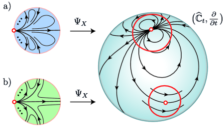
Figure 3. (a) Elliptic tracts arise from the asymptotic value $\infty\in{\widehat{\mathbb{C}}}_{t}$. (b) Hyperbolic tracts arise from finite asymptotic values $a_{\sigma}\in{\widehat{\mathbb{C}}}_{t}$. The asymptotic values $a_{\sigma}$, $\infty$ are represented by small red circles.

Proof.

Let $a\in{\widehat{\mathbb{C}}}_{t}$ be a singular (critical or asymptotic) value of $\Psi_{X}$. Since $\Psi_{X}$ is the global flow box of the associated vector field $X$, then the germ of $X$ is

(8) $$(U_{a}(\rho),X)=\Big{(}\Psi^{-1}_{X}\big{(}D(a,\rho)\backslash\{a\}\big{)},\Psi^{*}_{X}(\frac{\partial}{\partial t})\Big{)}\ \ \text{ for }a\in{\mathbb{C}}_{t}$$

or

(9) $$(U_{\infty}(\rho),X)=\Big{(}\Psi^{-1}_{X}\big{(}D(a,\rho)\backslash\{a\}\big{)},\Psi^{*}_{X}(-t^{2}\frac{\partial}{\partial t})\Big{)}\ \ \text{ for }a=\infty\in{\widehat{\mathbb{C}}}_{t}.$$

Clearly, cases (1)–(2) are algebraic singularities of $\Psi_{X}^{-1}$ and $\Psi_{X}$ is locally $k:1$ over $D(a,\rho)\backslash\{a\}$, where $k\geq 2$.

For $a\in{\mathbb{C}}_{t}$ it follows that $(U_{a}(\rho),X)$ has $2k$ hyperbolic sectors and hence is a vicinity of a pole $p$, according to Proposition 2.8, assertion 4.

On the other hand, $(U_{\infty}(\rho),X)$ has $2k$ elliptic (with possibly parabolic) sectors, hence is a vicinity of a zero $q$ of $X$; according to Proposition 2.8, assertion 3.

Let us examine assertions (3) & (4), they are transcendental singularities of $\Psi_{X}^{-1}$. They correspond to essential singularities of $X$, so $\Psi_{X}$ is locally $\infty:1$ over $D(a,\rho)\backslash\{a\}$.

In the case of a finite asymptotic value $a\in{\mathbb{C}}_{t}$, the germ of $X$ is $\big{(}U_{a}(\rho),\Psi^{*}(\frac{\partial}{\partial t})\big{)}$ and $U_{a}(\rho)$ contains an infinite union of hyperbolic sectors.

On the other hand, when $a=\infty$, the germ of $X$ is $\big{(}U_{\infty}(\rho),\Psi_{X}^{*}(-t^{2}\frac{\partial}{\partial t})\big{)}$ and $U_{a}(\rho)$ contains an infinite union of elliptic sectors or a parabolic sector. ∎

According to Table 1, the point $q\in M$ is a simple pole of $\Psi_{X}$ if and only if $X$ has a double zero at $q$.

The following distinction among direct transcendental singularities is well known.

Definition 3.8.

1. The transcendental singularity $U_{a}$ is a logarithmic singularity over $a$ if $\Psi_{X}:U(\rho)\longrightarrow D(a,\rho)\backslash\{a\}$ is a universal covering for some $\rho>0$. The (unbounded) neighborhoods $U(\rho)\subset{\widehat{\mathbb{C}}}$ are called exponential tracts of $U_{a}$.

Naturally, logarithmic singularities are direct, a careful look at the exponential vector field is useful.

Example 3.1.

The simplest case of a direct singularity arises from

$\Psi_{X}(z)=\int^{z}{\text{\myfont e}}^{-\zeta}d\zeta:{\mathbb{C}}_{z}\longrightarrow{\mathbb{C}}_{t}\backslash\{0\}$,

having

$X(z)={\text{\myfont e}}^{z}\frac{\partial}{\partial z}$

as its associated vector field. There are two logarithmic singularities over $0$ and $\infty$, respectively. There are two exponential tracts, moreover introducing the phase portrait of the associated vector field they can be clearly distinguished. Thus, three geometric pieces appear, Figures 3 and 4 provide heuristic arguments.

A hyperbolic tract $U_{0}(\rho)=\{{\mathfrak{Re}\left(z\right)}>\log(1/\left\lvert\rho\right\rvert)\}$ over the asymptotic value zero.

An elliptic tract $U_{\infty}(\rho)=\{{\mathfrak{Re}\left(z\right)}<\log(1/\left\lvert\rho\right\rvert)\}$ over the asymptotic value $\infty$.

A pairing of the asymptotic values $0$ and $\infty$ given by an entire sector $\mathscr{E}=\big{(}(\overline{{\mathbb{H}}}^{2},\infty),{\text{\myfont e}}^{z}\frac{\partial}{\partial z}\big{)}$.

In particular, the extension of $U_{0}(\rho)$ and $U_{\infty}(\rho)$ determines two entire sectors at $\infty$, denoted as $\mathscr{E}\mathscr{E}$.

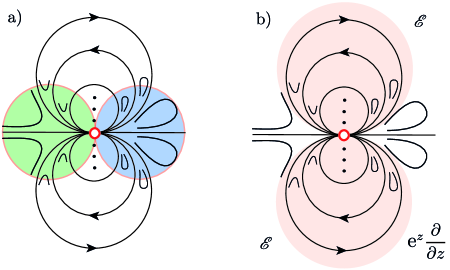
Figure 4. Geometry of the exponential vector field $X(z)={\text{\myfont e}}^{z}\frac{\partial}{\partial z}$. (a) The finite asymptotic value $0\in{\mathbb{C}}_{t}$ gives rise to two logarithmic singularities; one hyperbolic tract over $0$ (coloured green), and one elliptic tract over $\infty\in{\widehat{\mathbb{C}}}_{t}$ (coloured blue). (b) The singularity leads to two entire sectors $\mathscr{E}$ (coloured pink). There is a pairing of the asymptotic values, provided by an entire sector $\mathscr{E}$.

As an advantage of the existence of a vector field $X$ associated to a function $\Psi_{X}$, we can refine exponential tracts.

Definition 3.9.

1. The pairs

$\mathscr{U}_{H}=\big{(}\{{\mathfrak{Re}\left(z\right)}>0\},{\text{\myfont e}}^{z}\frac{\partial}{\partial z}\big{)}$,    $\mathscr{U}_{E}=\big{(}\{{\mathfrak{Re}\left(z\right)}<0\},{\text{\myfont e}}^{z}\frac{\partial}{\partial z}\big{)}$

are the hyperbolic tract over 0 and elliptic tract over $\infty$ of $\Psi_{X}(z)=-{\text{\myfont e}}^{-z}$, respectively. See Figure 3.

2. The pair $\big{(}U_{a}(\rho),X\big{)}$ is a hyperbolic tract over $a$ or elliptic tract over $a$ if there is a biholomorphism mapping $(U_{a}(\rho),X)$ to $\mathscr{U}_{H}$ or $\mathscr{U}_{E}$, respectively.

Certainly, the notion of biholomorphism is rigid. It is suitable for our present work since we gain flexibility of this notion by applying it to open Jordan domains of $(M,X)$ and under variations of the radius $\rho$. Since transcendental singularities can be very complex, not much can be said in general of their geometric structure. However, if we restrict ourselves to (direct) logarithmic transcendental singularities, then a clear picture arises.

Proposition 3.10.

Let $\Psi_{X}:M\longrightarrow{\widehat{\mathbb{C}}}_{t}$ be a transcendental meromorphic function with an essential singularity at $e\in M$.

1. The transcendental singularity $U_{a}$ of $\Psi^{-1}_{X}$ is logarithmic over a finite asymptotic value $a\in{\mathbb{C}}_{t}$ if and only if $\big{(}U_{a}(\rho),X\big{)}$ is a hyperbolic tract for sufficiently small $\rho>0$.

2. The transcendental singularity $U_{a}$ of $\Psi^{-1}_{X}$ is logarithmic over $a=\infty\in{\widehat{\mathbb{C}}}_{t}$ if and only if $\big{(}U_{a}(\rho),X\big{)}$ is an elliptic tract for sufficiently small $\rho>0$.

Proof.

$(\Rightarrow)$: Since $\Psi_{X}^{-1}$ has a logarithmic singularity over the asymptotic value $a$, then $\Psi_{X}:U_{a}(\rho)\longrightarrow D(a,\rho)\backslash\{a\}$ is a universal cover.

In the case $a\in{\mathbb{C}}_{t}$, the germ of $X$ is $\big{(}U_{a}(\rho),\Psi^{*}(\frac{\partial}{\partial t})\big{)}$, which is a hyperbolic tract.

On the other hand, when $a=\infty$, the germ of $X$ is $\big{(}U_{\infty}(\rho),\Psi_{X}^{*}(-t^{2}\frac{\partial}{\partial t})\big{)}$, which is an elliptic tract.

$(\Leftarrow)$: Definition 3.9.2 assumes the existence of a component $U_{a}(\rho)$ of $\Psi^{-1}_{X}\big{(}D(a,\rho)\big{)}$ such that $\rho_{1}<\rho_{2}\leq\rho$ implies $U_{a}(\rho_{1})\subset U_{a}(\rho_{2})$. Thus, $\big{(}U_{a}(\rho_{1}),X)$ and $\big{(}U_{a}(\rho_{2}),X\big{)}$ inherit the same type (hyperbolic or elliptic) of tract as $\big{(}U_{a}(\rho),X\big{)}$.

Secondly, because of the biholomorphism, say $\varphi$, from $\big{(}U_{a}(\rho),X\big{)}$ to $\mathscr{U}_{H}$ or $\mathscr{U}_{E}$, we have the following commuting diagrams

where $T_{j}:D(0,1)\longrightarrow D(a,\rho)$, for $j=1,2$, are appropriate biholomorphisms between the disks.

Hence, $\Psi_{X}:U_{a}(\rho)\longrightarrow D(a,\rho)\backslash\{a\}$ is a universal covering. ∎

Corollary 3.11.

Let $\Psi_{X}:M\longrightarrow{\widehat{\mathbb{C}}}_{t}$ be a transcendental meromorphic function with an essential singularity at $e\in M$ and further suppose that $U_{a}$ is a direct transcendental singularity of $\Psi^{-1}_{X}$ over the asymptotic value $a\in{\widehat{\mathbb{C}}}_{t}$. If $U_{a}(\rho)$ is not a hyperbolic or elliptic tract over $a$, for sufficiently small $\rho>0$, then $U_{a}$ is direct non logarithmic. ∎

As motivation, let us recall the following well known theorem [33] Ch. XI, §1.3., [36], [43] p. 231, which is a direct consequence of the normal form for holomorphic covers of the punctured plane.

Theorem (Isolated singular values).

Let $\Psi_{X}:{\mathbb{C}}_{z}\longrightarrow{\widehat{\mathbb{C}}}_{t}$ be a transcendental meromorphic function and let $a$ be an isolated singular value for $\Psi_{X}$. If $U_{a}$ is a singularity of $\Psi^{-1}_{X}$ over $a$, then $U_{a}$ is algebraic or logarithmic. $\Box$

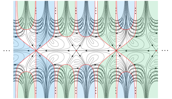
Figure 7. A function $\Psi_{X}(z)={\text{\myfont e}}^{\sin(z)-z}$ having an infinite number of algebraic and logarithmic singularities and two direct non logarithmic singularities. We sketch the phase portrait of the vector field $X(z)=\frac{{\text{\myfont e}}^{\sin(z)-z}}{\cos(z)-1}\frac{\partial}{\partial z}$. There are an infinite number of double poles of $X$ at $\{2\pi k\ |\ k\in{\mathbb{Z}}\}$ having $\{{\text{\myfont e}}^{-2\pi k}\ |\ k\in{\mathbb{Z}}\}$ as critical values of $\Psi_{X}$, and an infinite number of logarithmic singularities with asymptotic values $0$ and $\infty$. Moreover, there are two direct non logarithmic singularities over $0$ and $\infty$ with asymptotic paths ${\mathbb{R}}^{+}$ and ${\mathbb{R}}^{-}$, respectively.

As an immediate consequence, direct non logarithmic and indirect singularities of $\Psi^{-1}_{X}$ over $a$ imply that $a$ is non isolated, i.e. $a$ is an accumulation point of singular values of $\Psi_{X}$. There are, however, logarithmic singularities of $\Psi^{-1}_{X}$ over non isolated asymptotic values $a$, see for instance Example 4.6 and its corresponding Figure 7.

By using the perspective of vector fields, we shall prove a stronger version of the above theorem. We introduce the following concept.

Definition 3.12.

Let $U_{a}$ and $U_{b}$ be singularities of $\Psi^{-1}_{X}$ over the singular values $a$ and $b$, respectively.

1. The singularities $U_{a}$ and $U_{b}$ are separable if there are $\rho_{1},\rho_{2}>0$ such that their neighborhoods satisfy

$U_{a}(\rho_{1})\cap U_{b}(\rho_{2})=\varnothing$.

2. We shall say that the singularity $U_{a}$ is separate if given any other singularity $U_{b}$ of $\Psi^{-1}_{X}$ over $b$, $U_{a}$ and $U_{b}$ are separable.

Of course $a$ and $b$ can be the same singular value and yet $U_{a}$ and $U_{b}$ can be different singularities of $\Psi^{-1}_{X}$.

We can now prove the following.

Theorem 1.1.

Let $\Psi_{X}:M\longrightarrow{\widehat{\mathbb{C}}}_{t}$ be a transcendental meromorphic function with an essential singularity at $e\in M$. A singularity $U_{a}$ of $\Psi_{X}^{-1}$ is separate if and only if $U_{a}$ is algebraic or logarithmic.

Proof.

$(\Rightarrow)$ If $U_{a}$ is separate, then $D(a,\rho)\backslash\{a\}\,\cap\,D(b,\rho)\backslash\{b\}=\varnothing$ for all other singular values $b$. Thus $a$ is isolated.

$(\Leftarrow)$ Suppose to the contrary that $U_{a}$ is non separate. This means that there exists at least one singularity $U_{b}$ distinct from $U_{a}$ such that $U_{a}$ and $U_{b}$ are non separable, i.e. for any $\rho_{1},\rho_{2}>0$ there are neighborhoods $U_{a}(\rho_{1})\cap U_{b}(\rho_{2})\neq\varnothing$.

Since $U_{a}$ is logarithmic (the algebraic case is left to the reader), then for small enough $\rho_{1}>0$, $U_{a}(\rho_{1})$ is a hyperbolic or elliptic tract. In any of these cases $U_{a}(\rho_{1})$ does not contain any critical points and the only asymptotic paths that are completely contained in $U_{a}(\rho_{1})$ are those with asymptotic value $a$.

If $b$ is a critical value of $\Psi_{X}$, consider the critical point $c\in{\mathbb{C}}_{z}$ corresponding to $b$, then for small enough $\rho_{2}$,

$c\in U_{b}(\rho_{2})\subset U_{a}(\rho_{1})$ or $U_{a}(\rho_{1})\cap U_{b}(\rho_{2})=\varnothing$,

both of which lead to contradiction.

If $b$ is an asymptotic value of $\Psi_{X}$ then by considering a point

$z_{0}\in U_{a}(\rho_{1})\cap U_{b}(\rho_{2})\neq\varnothing$,

choose an asymptotic path $\alpha_{b}(\tau)$ of $U_{b}$ that starts at $z_{0}$, then one of the following holds true

(i) the whole asymptotic path $\alpha_{b}$ is contained in $U_{a}(\rho_{1})$,

(ii) otherwise there is a $\widetilde{\rho}_{2}>0$ smaller than $\rho_{2}$ such that $U_{a}(\rho_{1})\cap U_{b}(\widetilde{\rho}_{2})=\varnothing$.

Once again, both lead to contradiction. ∎

Remark 3.13 (Geometric behavior of singularities of $\Psi^{-1}_{X}$).

Let $a\in{\mathbb{C}}_{t}$ and $\infty$ denote singular values of $\Psi_{X}$.

1. The algebraic singularities $U_{a}$ and $U_{\infty}$ have their neighborhoods $U_{a}(\rho)$ and $U_{\infty}(\rho)$ composed of hyperbolic and elliptic sectors, respectively, as in Proposition 2.8.

2. The transcendental singularities of $\Psi_{X}^{-1}$ are further divided into three types: direct logarithmic, direct non logarithmic and indirect.

3. Direct logarithmic singularities $U_{a}$ and $U_{\infty}$ have neighborhoods $U_{a}(\rho)$ and $U_{\infty}(\rho)$ that are hyperbolic and elliptic tracts, respectively. See Proposition 3.10.

4. For $\Psi_{X}$ of finite order, $a\in{\widehat{\mathbb{C}}}_{t}$ is an asymptotic value of $\Psi_{X}$ that is an accumulation point of critical values of $\Psi_{X}$ if and only if $U_{a}$ is an indirect singularity of $\Psi_{X}^{-1}$. See [7] theorem 1.

The following inmediate result of Theorem 1.1 improves on Remark 3.13.4

Corollary 3.14.

A transcendental singularity $U_{a}$ of $\Psi_{X}^{-1}$ is non logarithmic if and only if $U_{a}$ is non separate. ∎

4. Holomorphic families and sporadic examples

4.1. Exponential families

The Speiser class, [37], consists of transcendental entire functions for which the singular values are a finite set (the closure of the critical values and finite asymptotic values). In particular, the family of entire functions with at most a finite number of logarithmic singularities is a cornerstone of the theory. A first analytic characterization due to R. Nevanlinna is the following.

Theorem 4.1 ([33] Ch. XI).

Entire functions $\Psi_{X}$ whose Schwarzian derivatives are degree ${\tt p}-2$ polynomials are precisely functions that have $\tt p$ logarithmic singularities.

Recall the pioneering work of E. Hille [22] and M. Taniguchi [40], [41]; see R. Devaney [9] §10 for a modern study. For the relations with the theory of the linear differential equation $y^{\prime\prime}-P(z)y=0$, see [38] pp. 156–157.

We consider

(10) $${\mathscr{E}}(r,d)=\left\{X(z)=\frac{1}{P(z)}{\text{\myfont e}}^{E(z)}\frac{\partial}{\partial z}\ \Big{|}\ P,\,E\in{\mathbb{C}}[z]\hbox{ of degree }r,\,d\geq 1\right\},$$

whose corresponding functions $\Psi_{X}$ are in the Speiser class. Note that each ${\mathscr{E}}(r,d)$ is a holomorphic family of complex dimension $r+d+1$.

Theorem 4.2 (The families ${\mathscr{E}}(r,d)$).

Let

(11) $$\Psi_{X}(z)=\int^{z}P(\zeta){\text{\myfont e}}^{-E(\zeta)}d\zeta$$

be the entire function arising from $X(z)\in{\mathscr{E}}(r,d)$.

1. $\Psi_{X}$ has $r$ critical values and $2d$ asymptotic values (all counted with multiplicity); $d$ finite values and $d$ over $\infty$.

2. All the singularites are logarithmic and separate.

3. There is a pairing of asymptotic values given by entire sectors $\mathscr{E}$. Furthermore each finite asymptotic value $a_{\sigma}\in{\mathbb{C}}_{t}$ gives rise to two logarithmic singularities, one over $a_{\sigma}$ (hyperbolic tract) and the other over $\infty\in{\widehat{\mathbb{C}}}_{t}$ (elliptic tract).

4. The isolated essential singularity at $\infty\in{\widehat{\mathbb{C}}}_{z}$ is the $\alpha$ or $\omega$–limit point of an infinite number of incomplete trajectories.

Proof.

Here we provide a sketch of the proof, see [4] for full details.

The associated single valued function is $\Psi_{X}(z)$, having $2d$ tracts at $\infty$. The singular values are isolated, hence all the transcendental singularities of $\Psi^{-1}_{X}$ are logarithmic.

In fact, the Riemann surface ${\mathcal{R}}_{X}$ can be constructed by a surgery procedure as follows. First, consider the Riemann surface of a suitable rational function $R(z):{\widehat{\mathbb{C}}}_{z}\longrightarrow{\widehat{\mathbb{C}}}_{t}$ with $r$ ramification points. Secondly, add hyperbolic tracts at $d$ cross cuts on the Riemann surface of $R(z)$.

The surgery idea first appeared in [40], moreover an approximation technique is developed in [4] §4.3.

The pairing is equivalent to the fact that the phase portrait of the singular vector field ${\mathfrak{Re}\left(X\right)}$ at $\infty\in{\widehat{\mathbb{C}}}_{z}$ has exactly $2d$ entire sectors $\mathscr{E}$, see for instance [3] theorem 12.2.

The last statement follows directly from Proposition 3.10. An alternative proof may be found in [2] theorem 9.1, which shows that these vector fields have $2d$ entire sectors, and that each entire sector is comprised of a hyperbolic tract and an elliptic tract. ∎

The vector fields ${\mathscr{E}}(0,2)$ and $X(z)={\text{\myfont e}}^{z^{d}}\frac{\partial}{\partial z}\in{\mathscr{E}}(0,d)$ for $d>2$ were studied by K. Hockett et al. [23], using real vector field methods, also see [20].

4.2. Families of periodic vector fields

A second large class of vector vector fields that give rise to holomorphic families is the periodic vector field class on ${\mathbb{C}}_{z}$, which include several trigonometric examples.

On ${\widehat{\mathbb{C}}}_{z}$ there exists a correspondence between

$\mathchoice{\mathbin{\vbox{\hbox{\scalebox{0.5}{$\displaystyle\bullet$}}}}}{\mathbin{\vbox{\hbox{\scalebox{0.5}{$\textstyle\bullet$}}}}}{\mathbin{\vbox{\hbox{\scalebox{0.5}{$\scriptstyle\bullet$}}}}}{\mathbin{\vbox{\hbox{\scalebox{0.5}{$\scriptscriptstyle\bullet$}}}}}$ singular complex analytic vector fields $X$ on ${\widehat{\mathbb{C}}}_{z}$ of period $T\in{\mathbb{C}}^{*}$ with $\omega_{X}$ having zero residues, and

$\mathchoice{\mathbin{\vbox{\hbox{\scalebox{0.5}{$\displaystyle\bullet$}}}}}{\mathbin{\vbox{\hbox{\scalebox{0.5}{$\textstyle\bullet$}}}}}{\mathbin{\vbox{\hbox{\scalebox{0.5}{$\scriptstyle\bullet$}}}}}{\mathbin{\vbox{\hbox{\scalebox{0.5}{$\scriptscriptstyle\bullet$}}}}}$ singular complex analytic functions $\Psi_{X}$ of period $T$.

Moreover, in such a case,

(12) $$\Psi_{X}(z)=h\circ{\text{\myfont e}}^{2\pi iz/T}$$

is single valued, where $h$ is a suitable singular complex analytic function. Among the periodic examples, the “simplest” ones are those obtained when considering $h=R$ a rational function, as follows.

Theorem 4.3.

Let $X$ be singular complex analytic vector field on ${\widehat{\mathbb{C}}}_{z}$ arising from the distinguished parameter $\Psi_{X}$ in the family

$$\mathscr{P}_{\tt r}\doteq\left\{\Psi_{X}(z)=R\circ{\text{\myfont e}}^{2\pi iz/T}\ \big{|}\ R:{\widehat{\mathbb{C}}}\longrightarrow{\widehat{\mathbb{C}}}_{t}\text{ rational of degree }{\tt r}\geq 1\right\}.$$

The following assertions hold.

1. $X$ is periodic of period $T\in{\mathbb{C}}^{*}$ with a unique essential singularity at $\infty\in{\widehat{\mathbb{C}}}_{z}$.

2. $\Psi_{X}$ has two asymptotic values $a_{0}\doteq R(0)$ and $a_{\infty}\doteq R(\infty)$, counted with multiplicity.

3. Each of the two transcendental singularities of $\Psi^{-1}_{X}$ is logarithmic. The corresponding exponential tracts are

   1. hyperbolic tracts when the asymptotic value is finite, and

   2. elliptic tracts when the asymptotic value is $\infty$.

4. If the critical point set $\mathcal{C}_{R}\subset{\widehat{\mathbb{C}}}_{z}$ of $R$ satisfies that $\mathcal{C}_{R}\backslash\{0,\infty\}\neq\varnothing$, then $X$ has an infinite number of poles accumulating at $\infty\in{\widehat{\mathbb{C}}}_{z}$.

5. If $\infty\in{\widehat{\mathbb{C}}}_{t}$ is not an asymptotic value, then $X$ has an infinite number of zeros of multiplicty 2 and residue zero accumulating at $\infty\in{\widehat{\mathbb{C}}}_{z}$.

6. The configuration of the two asymptotic values and infinity

   $\{a_{0},a_{\infty},\infty\}\subset{\widehat{\mathbb{C}}}_{t}$

   provides a decomposition of the family $\mathscr{P}_{\tt r}$ into four subfamilies.

   1. (Generic case) Three distinct points $\{a_{0},a_{\infty},\infty\}$.

   2. Two distinct points $\{a_{0}=a_{\infty},\,\infty\}$.

   3. Two distinct points $\{a_{0},\,a_{\infty}=\infty\}$   or   $\{a_{0}=\infty,\,a_{\infty}\}$.

   4. One distinct point $\{a_{0}=a_{\infty}=\infty\}$.

As usual, generic means an open and dense set in the space of parameters of $\mathscr{P}_{\tt r}$.

Proof.

The space of rational functions $R(w)$ of degree ${\tt r}\geq 1$ is an open Zariski set in $\mathbb{CP}^{2{\tt r}+1}$, hence $\mathscr{P}_{\tt r}$ inherits this open complex manifold structure.

Without loss of generality, assume that the period is $T=2\pi i$. Under pullback we have a diagram

(13) $$({\widehat{\mathbb{C}}}_{z},X)\stackrel{{\scriptstyle{\text{\myfont e}}^{z}}}{{\longrightarrow}}\big{(}{\widehat{\mathbb{C}}}_{w},R^{*}\frac{\partial}{\partial t}\big{)}\stackrel{{\scriptstyle R}}{{\longrightarrow}}\big{(}{\widehat{\mathbb{C}}}_{t},\frac{\partial}{\partial t}\big{)}\,.$$

Here $R^{*}\frac{\partial}{\partial t}$ is a rational vector field with

$\mathchoice{\mathbin{\vbox{\hbox{\scalebox{0.5}{$\displaystyle\bullet$}}}}}{\mathbin{\vbox{\hbox{\scalebox{0.5}{$\textstyle\bullet$}}}}}{\mathbin{\vbox{\hbox{\scalebox{0.5}{$\scriptstyle\bullet$}}}}}{\mathbin{\vbox{\hbox{\scalebox{0.5}{$\scriptscriptstyle\bullet$}}}}}$ zeros of order $\geq 2$ and residue zero, at the poles of $R$, and

$\mathchoice{\mathbin{\vbox{\hbox{\scalebox{0.5}{$\displaystyle\bullet$}}}}}{\mathbin{\vbox{\hbox{\scalebox{0.5}{$\textstyle\bullet$}}}}}{\mathbin{\vbox{\hbox{\scalebox{0.5}{$\scriptstyle\bullet$}}}}}{\mathbin{\vbox{\hbox{\scalebox{0.5}{$\scriptscriptstyle\bullet$}}}}}$ poles at the critical points of $R$ in ${\mathbb{C}}^{*}_{w}$ with finite critical values.

From the above observations statements (4) and (5) follow.

Statement (1) follows from the periodicity and essential singularity of ${\text{\myfont e}}^{z}$.

Statement (2) follows from noting that the asymptotic values of ${\text{\myfont e}}^{z}$ are precisely $0$ and $\infty$, thus the asymptotic values of $\Psi_{X}$ are $a_{0}\doteq R(0)$ and $a_{\infty}\doteq R(\infty)$.

Note that $\Psi_{X}$ is the universal cover of a neighborhood of the transcendental singularity $U_{a}$ of $\Psi^{-1}_{X}$, namely

$U_{a}(\rho)=\Psi_{X}^{-1}\big{(}D(a,\rho)\big{)}=\log\Big{(}R^{-1}\big{(}D(a,\rho)\big{)}\Big{)}$,

for $a=a_{0},a_{\infty}$ and $\rho>0$ sufficiently small. Thus, statements (3.i) and (3.ii) follow from Proposition 3.10.

For statement (6), in accordance with Diagram 13, the behavior of $R$ provides a sharp description of the zeros and poles of $X$, as well as the exponential tracts of $\Psi_{X}$. A systematic description of the different subfamilies in $\mathscr{P}_{\tt r}$ is given by the configuration of the two asymptotic values and infinity.

i) Generic case. Three distinct points $\{a_{0},a_{\infty},\infty\}$.

Clearly, the above condition defines a generic set in $\mathscr{P}_{\tt r}$. Moreover, $X$ has an infinite number of zeros of multiplicity at least 2 and residue zero accumulating at $\infty\in{\widehat{\mathbb{C}}}_{z}$. In addition, if the critical point set of $R$ is different from $0$ or $\infty$, then $X$ has an infinite number of poles accumulating at $\infty\in{\widehat{\mathbb{C}}}_{z}$. Finally, the neighborhoods $U_{a_{0}}(\rho)$ and $U_{a_{\infty}}(\rho)$ of the singularities of $\Psi^{-1}_{X}$ will be hyperbolic tracts. See Example 4.1.

ii) Two different points $\{a_{0}=a_{\infty},\,\infty\}$.

Since $a=a_{0}=a_{\infty}\neq\infty$, then $\Psi_{X}$ has one finite asymptotic value $a\in{\mathbb{C}}_{t}$ of multiplicity 2, i.e. two logarithmic branch points over the same finite asymptotic value $a$.

By necessity, $\Psi_{X}$ has at least another branch point over $b\in{\widehat{\mathbb{C}}}\backslash\{a\}$, which can’t be transcendental. Thus, $b$ must be a critical value.

If $b\neq\infty$, then $X$ has an infinite number of zeros of multiplicity at least 2 and residue zero accumulating at $\infty\in{\widehat{\mathbb{C}}}_{z}$.

If $b=\infty$, then $X$ also has an infinite number of poles accumulating at $\infty\in{\widehat{\mathbb{C}}}_{z}$.

Finally, the two neighborhoods $U_{a_{0}}(\rho)$ and $U_{a_{\infty}}(\rho)$ of the singularities of $\Psi^{-1}_{X}$ will be hyperbolic tracts. Let

(14) $$R(w)=\frac{c_{r}w^{r}+c_{r-1}w^{r-1}+\cdots+c_{1}w+c_{0}}{b_{s}w^{s}+b_{s-1}w^{s-1}+\cdots+b_{1}w+b_{0}},\ \ \ {\tt r}=\max\{r,\,s\},$$

be a rational function. A straightforward calculation shows that either

(15) $$r=s\ \hbox{ and }\ \dfrac{c_{r}}{b_{r}}=\dfrac{c_{0}}{b_{0}},\ \hbox{ so }\ a=R(\infty)=R(0)=\dfrac{c_{0}}{b_{0}}\in{\mathbb{C}}^{*}_{t},$$

or

(16) $$s>r\ \hbox{ and }\ a=R(\infty)=R(0)=0,\text{ in particular }c_{0}=0\text{ in }\eqref{funcion-racional}.$$

See Example 4.2.

iii) Two different points $\{a_{0},\,a_{\infty}=\infty\}$   or   $\{a_{0}=\infty,\,a_{\infty}\}$.

The vector field $X$ will not have any zeros. If $\mathcal{C}_{R}\backslash\{0,\infty\}\neq\varnothing$, then $X$ has an infinite number of poles accumulating at $\infty\in{\widehat{\mathbb{C}}}_{z}$. One of the neighborhoods of the singularities of $\Psi^{-1}_{X}$ will be a hyperbolic tract and the other will be an elliptic tract. In particular, Equation (14) requires

(17) $$s<r\ \hbox{ and }\ a_{0}=R(0)=\dfrac{c_{0}}{b_{0}}\in{\mathbb{C}}_{t},\ a_{\infty}=R(\infty)=\infty.$$

The other option is given by considering the rational function $\widehat{R}(w)=R(1/w)$ with $R$ as in (17), so $a_{0}=\widehat{R}(0)=\infty$ and $a_{\infty}=\widehat{R}(\infty)\in{\mathbb{C}}_{t}$.

See Example 4.3.

iv) One distinct point $\{a_{0}=a_{\infty}=\infty\}$.

Note that, $X$ will have no zeros. If $\mathcal{C}_{R}\backslash\{0,\infty\}\neq\varnothing$, then $X$ has an infinite number of poles accumulating at $\infty\in{\widehat{\mathbb{C}}}_{z}$. The two neighborhoods $U_{a_{0}}(\rho)$ and $U_{a_{\infty}}(\rho)$ of the singularities of $\Psi^{-1}_{X}$ will be elliptic tracts. In this case

(18) $$s<r\ \hbox{ and }\ R(0)=R(\infty)=\infty\in{\widehat{\mathbb{C}}}_{t},\text{ in particular }b_{0}=0\text{ in }\eqref{funcion-racional}.$$

See Example 4.4. ∎

Example 4.1 (Two logarithmic singularities over finite asymptotic values).

The vector field

$X(z)=\big{(}\cos(z)+1\big{)}\frac{\partial}{\partial z}=2\cos^{2}(\frac{z}{2})\frac{\partial}{\partial z}$

is such that

$\Psi_{X}(z)=\tan(\frac{z}{2})=-i\frac{{\text{\myfont e}}^{iz}-1}{{\text{\myfont e}}^{iz}+1}=-i\frac{w-1}{w+1}\circ{\text{\myfont e}}^{iz}$,

so it falls under the hypothesis of Theorem 4.3, Case 6.i. Thus, $R(w)=-i(w-1)/(w+1)$ and $-i,\,i\in{\mathbb{C}}_{t}$ are the finite asymptotic values of $\Psi_{X}$. There are two logarithmic singularities of $\Psi^{-1}_{X}$ over $-1$, $1\in{\mathbb{C}}_{t}$, with neighborhoods corresponding to the (open) upper and lower half planes. Each is a hyperbolic tract. In this case, $X$ has an infinite number of double zeros and no poles. See Figure 5.a.

Example 4.2.

The vector field

$X(z)=-2i\dfrac{\sin^{2}(z)}{\cos(z)}\frac{\partial}{\partial z}$

is such that

$\Psi_{X}(z)=\dfrac{1}{2i}\dfrac{1}{\sin(z)}=\dfrac{1}{w+w^{-1}}\circ{\text{\myfont e}}^{iz}$,

so it falls under the hypothesis of Theorem 4.3, Case 6.ii. Since $R(w)=w/(w^{2}+1)$ takes $0,\,\infty$ to $0$, then $0\in{\mathbb{C}}_{t}$ is the finite asymptotic value of $\Psi_{X}$ of multiplicity 2. There are two logarithmic singularities of $\Psi^{-1}_{X}$ over $0\in{\mathbb{C}}_{t}$, with neighborhoods corresponding to the (open) upper and lower half planes. Each is a hyperbolic tract. There are an infinite number of zeros of order 2 and an infinite number of simple poles alternating on the real axis, both accumulating at $\infty\in{\widehat{\mathbb{C}}}_{z}$.

Example 4.3.

As an example of Theorem 4.3, Case 6.iii, consider a polynomial $R=P$, thus

$\Psi_{X}(z)=P({\text{\myfont e}}^{z})\ \ \ \hbox{and}\ \ \ X(z)=\dfrac{1}{{\text{\myfont e}}^{z}P^{\prime}({\text{\myfont e}}^{z})}\frac{\partial}{\partial z},$

which has a logarithmic singularity over the finite asymptotic value $P(0)\in{\mathbb{C}}_{t}$ (hyperbolic tract) and a logarithmic singularity over $\infty\in{\widehat{\mathbb{C}}}_{t}$ (elliptic tract). If the critical point set $\mathcal{C}_{P}$ satisfies $\mathcal{C}_{P}\backslash\{0,\infty\}\neq\varnothing$, then the poles of $X$ are the infinite solutions of $P^{\prime}({\text{\myfont e}}^{z})=0$. As a second option $\widehat{R}(0)=\infty$ and $\widehat{R}(\infty)=0$, in this case we use $\widehat{R}(w)=P(1/w)$ and analogous arguments.

Example 4.4 (Two logarithmic singularities over $\infty$).

The vector field

$X(z)=\sec(z)\frac{\partial}{\partial z}$

is such that

$\Psi_{X}(z)=\sin(z)=\dfrac{w-w^{-1}}{2i}\circ{\text{\myfont e}}^{iz}$,

so it falls under the hypothesis of Theorem 4.3, Case 6.iv. Since $R(w)=(w-w^{-1})/2i$ takes $0,\infty\mapsto\infty$, then $\infty\in{\widehat{\mathbb{C}}}_{t}$ is an asymptotic value of multiplicity 2 and $\Psi_{X}$ has no finite asymptotic values. There are two logarithmic singularities of $\Psi^{-1}_{X}$ over $\infty\in{\widehat{\mathbb{C}}}_{t}$, with neighborhoods corresponding to the (open) upper and lower half planes. Each has an elliptic tract over $\infty$. Since $\int_{\pi/2}^{(3/2)\pi}\cos(\zeta)d\zeta$ is finite, the incomplete trajectories $z_{k}(\tau):(a,b)\subsetneq{\mathbb{R}}\to{\mathbb{C}}_{z}$ of $X$, having as images the real segments $(\pi/2+k\pi,(3/2)\pi+k\pi)\subset{\mathbb{R}}$, $k\in{\mathbb{Z}}$, are located at the poles $\{(1/2)\pi+k\}$ of $X$. See Figure 5.b.

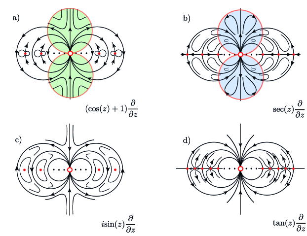
Figure 5. Vector fields on ${\widehat{\mathbb{C}}}$ near $\infty$ (represented by an small red circle). (a) $(\cos(z)+1)\frac{\partial}{\partial z}$ with an accumulation of double zeros. (b) $\sec(z)\frac{\partial}{\partial z}$ with an accumulation of simple poles. (c) $i\sin(z)\frac{\partial}{\partial z}$ with an accumulation of simple zeros. (d) $\tan(z)\frac{\partial}{\partial z}$ with an accumulation of simple zeros and poles. The shaded circular regions illustrate elliptic or hyperbolic tracts in (a) and (b). Note that (c) and (d) have multivalued $\Psi_{X}$.

4.3. Sporadic examples

Example 4.5 (An infinite number of logarithmic singularities but no direct non logarithmic or indirect singularities).

Let

$\Psi_{X}(z)={\text{\myfont e}}^{\sin(z)}$.

The associated vector field is

$X(z)=\dfrac{1}{\Psi_{X}^{\prime}(z)}\frac{\partial}{\partial z}=\dfrac{{\text{\myfont e}}^{-\sin(z)}}{\cos(z)}\frac{\partial}{\partial z}$.

See Figure 6. The critical points of $\Psi_{X}$ are $\{\frac{\pi}{2}(2k+1)\ |\ k\in{\mathbb{Z}}\}$ and its critical values are $\{{\text{\myfont e}},{\text{\myfont e}}^{-1}\}$.

The asymptotic values of $\Psi_{X}$ are $0$, $\infty$. Clearly, $0$ and $\infty$ are isolated asymptotic values, so the transcendental singularities are logarithmic.

By considering the phase portrait of $X$, it is clear that there are an infinite number of logarithmic singularities $U_{k\pm}$. Let $k\in{\mathbb{Z}}$, we have neighborhoods

$U_{k\pm}(\rho)=\{z\in{\mathbb{C}}_{z}\ |\ \left\lvert{\mathfrak{Re}\left(z\right)}-(2k+1)\frac{\pi}{2}\right\rvert<\pi,\ \pm{\mathfrak{Im}\left(z\right)}>R(\rho)\}$,

for appropriate $R(\rho)$, containing asymptotic paths $\alpha_{k\pm}(\tau)=(2k+1)\frac{\pi}{2}\pm i\tau$. We have the following dichotomy.

$\mathchoice{\mathbin{\vbox{\hbox{\scalebox{0.5}{$\displaystyle\bullet$}}}}}{\mathbin{\vbox{\hbox{\scalebox{0.5}{$\textstyle\bullet$}}}}}{\mathbin{\vbox{\hbox{\scalebox{0.5}{$\scriptstyle\bullet$}}}}}{\mathbin{\vbox{\hbox{\scalebox{0.5}{$\scriptscriptstyle\bullet$}}}}}$ For odd $k$, the asymptotic value is $0$ and $U_{k\pm}(\rho)$ is a hyperbolic tract over $0$.

$\mathchoice{\mathbin{\vbox{\hbox{\scalebox{0.5}{$\displaystyle\bullet$}}}}}{\mathbin{\vbox{\hbox{\scalebox{0.5}{$\textstyle\bullet$}}}}}{\mathbin{\vbox{\hbox{\scalebox{0.5}{$\scriptstyle\bullet$}}}}}{\mathbin{\vbox{\hbox{\scalebox{0.5}{$\scriptscriptstyle\bullet$}}}}}$ For even $k$, the asymptotic value is $\infty$ and $U_{k}(\rho)$ is an elliptic tract over $\infty$.

Also note that, along the real axis $\Psi_{X}(z)$ does not converge as $z\to\pm\infty$, i.e. there is no asymptotic path (or value) along the real axis. In particular, $\infty\in{\widehat{\mathbb{C}}}_{z}$ is a non isolated essential singularity of $X$.

Figure 6. Function $\Psi_{X}={\text{\myfont e}}^{\sin(z)}$ with an infinite number of logarithmic singularities and no direct non logarithmic or indirect singularities. Phase portrait of the vector field $X(z)=\sec(z){\text{\myfont e}}^{-\sin(z)}\frac{\partial}{\partial z}$. There are an infinite number of simple poles of $X$ at $\{(2k+1)\pi/2\ |\ k\in{\mathbb{Z}}\}$, having e and ${\text{\myfont e}}^{-1}$ as critical values of $\Psi_{X}$. Moreover, there are an infinite number of logarithmic singularities with asymptotic values corresponding to $0,\infty$. Note that there are no other singularities of $\Psi^{-1}_{X}$.

Example 4.6 (Direct non logarithmic singularity of $\Psi^{-1}_{X}$).

Let

$\Psi_{X}(z)={\text{\myfont e}}^{\sin(z)-z}$,

compare with [29]. The associated vector field is

$X(z)=\frac{1}{\Psi_{X}^{\prime}(z)}\frac{\partial}{\partial z}=\dfrac{{\text{\myfont e}}^{\sin(z)-z}}{\cos(z)-1}\frac{\partial}{\partial z}$.

The critical points of $\Psi_{X}$ are $\{2\pi k\ |\ k\in{\mathbb{Z}}\}$, with critical values $\{{\text{\myfont e}}^{-2\pi k}\ |\ k\in{\mathbb{Z}}\}$.

See Figure 4.6. The asymptotic values of $\Psi_{X}$ are $0$ and $\infty$. Note that they are non isolated singular values. Since $\Psi_{X}$ is entire and these are omitted values, the corresponding transcendental singularities are direct.

For each $k\in{\mathbb{Z}}$, the neighborhoods

$U_{k\pm}(\rho)=\left\{z\in{\mathbb{C}}_{z}\ |\ \left\lvert{\mathfrak{Re}\left(z\right)}-(2k+1)\frac{\pi}{2}\right\rvert<\pi,\ \pm{\mathfrak{Im}\left(z\right)}>R(\rho)\right\}$,

for appropriate $R(\rho)$, containing the asymptotic paths $\alpha_{k\pm}(\tau)=(2k+1)\frac{\pi}{2}\pm i\tau$, where $\tau>0$, are associated to the singularities $U_{k\pm}$.

Since these neighborhoods are mutually disjoint, the singularities are separate, so by Theorem 1.1 they are logarithmic. Once again we have a dichotomy below.

$\mathchoice{\mathbin{\vbox{\hbox{\scalebox{0.5}{$\displaystyle\bullet$}}}}}{\mathbin{\vbox{\hbox{\scalebox{0.5}{$\textstyle\bullet$}}}}}{\mathbin{\vbox{\hbox{\scalebox{0.5}{$\scriptstyle\bullet$}}}}}{\mathbin{\vbox{\hbox{\scalebox{0.5}{$\scriptscriptstyle\bullet$}}}}}$ For odd $k$, the asymptotic value is $0$ and $U_{k\pm}(\rho)$ is a hyperbolic tract.

$\mathchoice{\mathbin{\vbox{\hbox{\scalebox{0.5}{$\displaystyle\bullet$}}}}}{\mathbin{\vbox{\hbox{\scalebox{0.5}{$\textstyle\bullet$}}}}}{\mathbin{\vbox{\hbox{\scalebox{0.5}{$\scriptstyle\bullet$}}}}}{\mathbin{\vbox{\hbox{\scalebox{0.5}{$\scriptscriptstyle\bullet$}}}}}$ For even $k$, the asymptotic value is $\infty$ and $U_{k\pm}(\rho)$ is an elliptic tract.

Moreover, the asymptotic value $\infty$, arising from the asymptotic path $\alpha_{-}(\tau)$, having image ${\mathbb{R}}^{-}$, gives rise to a direct transcendental singularity of $\Psi^{-1}_{X}$, say $U_{\infty-}$. The corresponding neighborhoods are

$U_{\infty-}(\rho)=\{z\in{\mathbb{C}}_{z}\ |\ -\frac{\pi}{2}<\arg(\frac{1}{z})<\frac{\pi}{2},\ {\mathfrak{Re}\left(z\right)}<R(\rho)\}$,

for suitable $R(\rho)$.

Similarly, the asymptotic value $0$ arising from the asymptotic path $\alpha_{+}(t)$, having image ${\mathbb{R}}^{+}$, gives rise to a direct transcendental singularity of $\Psi^{-1}_{X}$, say $U_{\infty+}$. The corresponding neighborhoods are

$U_{\infty+}(\rho)=\{z\in{\mathbb{C}}_{z}\ |\ -\frac{\pi}{2}<\arg(\frac{1}{z})<\frac{\pi}{2},\ {\mathfrak{Re}\left(z\right)}>R(\rho)\}$,

for appropriate $R(\rho)$.

The neighborhoods $U_{\infty\pm}(\rho)$ are non separate. By Theorem 1.1, they correspond to direct non logarithmic singularities.

Example 4.7 (Indirect transcendental singularity of $\Psi^{-1}_{X}$).

Let

$\Psi_{X}(z)=\sin(z)/z$.

The associated vector field is

$X(z)=\frac{z^{2}}{z\cos(z)-\sin(z)}\frac{\partial}{\partial z}$.

The critical points of $\Psi_{X}$ are the unbounded set $\{z\in{\mathbb{C}}_{z}\ |\ z\cos(z)-\sin(z)=0\}$, with critical values lying on the real axis and converging to $0$ as the critical points approach $\pm\infty$.

The asymptotic values of $\Psi_{X}(z)$ are $0$ and $\infty$.

Since $\infty$ is an isolated asymptotic value, the singularities of $\Psi^{-1}_{X}$ over $\infty$ are logarithmic. In fact, there are two, say $U_{\infty\pm}$, arising from the asymptotic paths $\alpha_{\infty\pm}$ having images $i{\mathbb{R}}^{+}$ and $i{\mathbb{R}}^{-}$. The corresponding (disjoint) neighborhoods are

$U_{\infty\pm}(\rho)=\{z\in{\mathbb{C}}_{z}\ |\ \pm{\mathfrak{Im}\left(z\right)}>R(\rho)\}$,

for appropriate $R(\rho)>0$.

The neighborhoods $U_{\infty\pm}(\rho)$ are elliptic tracts.

On the other hand, since $\Psi_{X}$ assumes the value $0$ infinitely often along the real axis, the transcendental singularities of $\Psi^{-1}_{X}$ over $0$ are indirect. In fact, there are two: $U_{0\pm}$ arising from the asymptotic paths $\alpha_{0\pm}(\tau)$ having images ${\mathbb{R}}^{+}$ and ${\mathbb{R}}^{-}$.

The phase portrait of $X$ is topologically equivalent to the phase portrait of $\sec(z)\frac{\partial}{\partial z}$, see Figure 5.b. See for instance [3] §11 for accurate definitions.

Remark 4.4 (The topology of the vector field does not determine the nature of essential singularity of the singularity of $\Psi_{X}$).

Contrary to the case of algebraic singularities of $\Psi^{-1}_{X}$, for transcendental singularities, the previous example, shows that the vector fields

$X_{1}(z)=\frac{z^{2}}{z\cos(z)-\sin(z)}\frac{\partial}{\partial z}$   and  $X_{2}(z)=\sec(z)\frac{\partial}{\partial z}$

have the same topological phase portraits. However in terms of the singularities of $\Psi^{-1}_{X}$ they have important differences, $X_{1}$ has an indirect transcendental singularity, but $X_{2}$ does not. Furthermore, $\Psi_{X_{1}}$ has 4 asymptotic values $\{0,0,\infty,\infty\}$, but $\Psi_{X_{1}}$ only two, namely $\{\infty,\infty\}$.

Example 4.8 (Direct non logarithmic singularity without critical points).

Let

$\Psi_{X}(z)=\int\limits_{0}^{z}{\text{\myfont e}}^{-{\text{\myfont e}}^{\zeta}}d\zeta$,

see [21], [36]. The associated vector field is

$X(z)={\text{\myfont e}}^{{\text{\myfont e}}^{z}}\frac{\partial}{\partial z}$.

It is clear that the critical point set of $\Psi_{X}$ is empty.

Let $a_{0}=\lim\limits_{{\mathbb{R}}^{+}\ni\tau\to\infty}\Psi_{X}(\tau)=-\int\limits_{-1}^{\infty}\frac{e^{-t}}{t}\,dt\approx 0.219384$. There are an infinite number of finite asymptotic values of $\Psi_{X}$ given by

$\{a_{k}\doteq a_{0}+i2k\pi\ |\ k\in{\mathbb{Z}}\}\subset{\mathbb{C}}_{t}$,

with asymptotic paths

$\{\alpha_{k}(\tau)=\tau+i2k\pi\ |\ k\in{\mathbb{Z}}\}$,    for $\tau\geq 0$,

in according to [21] p. 271.

Since the finite asymptotic values are isolated, the corresponding transcendental singularities of $\Psi^{-1}_{X}$ are logarithmic and their neighborhoods $U_{a_{k}}(\rho)$ are hyperbolic tracts over $a_{k}$.

On the other hand, the asymptotic paths

$\{\beta_{k}(\tau)=\tau+i(2k+1)\pi\ |\ k\in{\mathbb{Z}}\}$, for $\tau\geq 0$

have the asymptotic value $\infty\in{\widehat{\mathbb{C}}}_{t}$, in accordance with [21], statement (8). Note that $\infty$ is a non isolated asymptotic value. The asymptotic paths $\{\beta_{k}\}$ correspond to neighborhoods $U_{\infty,k}(\rho)$ that can be made disjoint from the neighborhoods of other singularities of $\Psi^{-1}_{X}$, thus these transcendental singularities are separate. Hence by Theorem 1.1, they are also logarithmic singularities of $\Psi^{-1}_{X}$. It follows that the neighborhoods $U_{\infty,k}(\rho)$ are elliptic tracts over $\infty$.

From statements (9) and (10) of [21], $\infty\in{\widehat{\mathbb{C}}}_{t}$ is an asymptotic value for asymptotic paths arriving to $\infty\in{\widehat{\mathbb{C}}}_{t}$ in an angular sector of angle $2\pi$ that avoids the positive real line. We shall denote by $U_{\infty,-}$ the corresponding singularity. For $\rho>0$, each neighborhood $U_{\infty,-}(\rho)$ contains an infinite number of neighborhoods $U_{a_{k}}(\rho)$ and $U_{\infty,k}(\rho)$, hence the singularity $U_{\infty,-}$ is non separate, thus direct non logarithmic. See Figure 8.

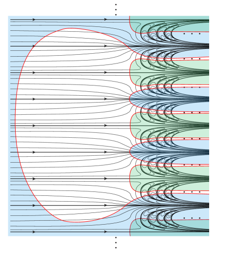
Figure 8. Phase portrait of the vector field $X(z)={\text{\myfont e}}^{{\text{\myfont e}}^{z}}\frac{\partial}{\partial z}$. In this case, there are an infinite number of logarithmic singularities with finite asymptotic values given by $a_{0}+i2k\pi$, with asymptotic paths $\alpha_{k}(\tau)=\tau+i2k\pi$, for $k\in{\mathbb{Z}}$. There are an infinite number of logarithmic singularities with asymptotic value $\infty\in{\widehat{\mathbb{C}}}_{t}$, with asymptotic paths $\beta_{k}(\tau)=\tau+i(2k+1)\pi$. Furthermore, there is a direct non logarithmic singularity $U_{\infty,-}$ over $\infty\in{\widehat{\mathbb{C}}}_{t}$, corresponding to asymptotic paths contained in an angular sector about $\infty\in{\widehat{\mathbb{C}}}_{t}$ that avoids the positive real axis.

Example 4.9 (Direct non logarithmic singularity of $\Psi^{-1}_{X}$ over asymptotic value that is an accumulation of critical values).

Let

$\Psi_{X}(z)={\text{\myfont e}}^{z}\sin({\text{\myfont e}}^{z})$.

The associated vector field is

$X(z)=\frac{1}{e^{z}\sin\left(e^{z}\right)+e^{2z}\cos\left(e^{z}\right)}\frac{\partial}{\partial z}$.

The critical points of $\Psi_{X}$ are the unbounded set

$\{z\in{\mathbb{C}}_{z}\ |\ {\text{\myfont e}}^{z}\Big{(}\sin\left({\text{\myfont e}}^{z}\right)+{\text{\myfont e}}^{z}\cos\left({\text{\myfont e}}^{z}\right)\Big{)}=0\}$,

which lie along the real lines of height $ik\pi$, $k\in{\mathbb{Z}}$ and whose real part is approximately given by $\{\log((2j+1)\frac{\pi}{2})\ |\ j\in{\mathbb{N}}\}$. Thus in particular, the critical points lie to the right of ${\mathfrak{Re}\left(z\right)}=\log(3\pi/2)\approx 1.55019$. The corresponding critical values lie on the real axis and converge to $-\infty$ as the critical points approach $\infty$.

The asymptotic values of $\Psi_{X}$ are $0,\infty\in{\widehat{\mathbb{C}}}_{t}$.

Since $a=0$ is an isolated asymptotic value, there is a (direct) logarithmic singularity $U_{0}$ over it. Its neighborhoods $U_{0}(\rho)$ are contained in half planes

$U_{0}(\rho)\subset\{z\in{\mathbb{C}}_{z}\ |\ {\mathfrak{Re}\left(z\right)}<-R(\rho)\}$,

for appropriate $R(\rho)>0$. The neighborhoods $U_{0}(\rho)$ are hyperbolic tracts over $0$.

On the other hand, since $\Psi_{X}$ is entire, $\infty$ is an omitted value, and hence the singularity $U_{\infty}$ associated to the asymptotic value $\infty$ is direct.

Note that any neighborhood $U_{\infty}(\rho)$ of this direct singularity contains a half plane $\{{\mathfrak{Re}\left(z\right)}>R(\rho)\}$, for appropriate $R(\rho)$, and thus an infinite number of critical points (algebraic singularities of $\Psi^{-1}_{X}$). Therefore $U_{\infty}$ is non separate, i.e. it is a direct non logarithmic singularity over $\infty$. Alternatively, to see that this singularity is direct non logarithmic, is to use Corollary 3.11 and “recognize” that the neighborhoods are not hyperbolic or elliptic tracts. See Figure 9.

It is to be noted that this $\Psi_{X}$ only has two transcendental singularities of $\Psi^{-1}_{X}$: a logarithmic singularity and a direct non logarithmic singularity.

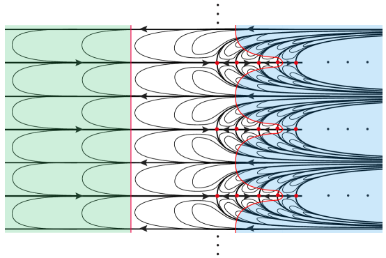
Figure 9. For $\Psi_{X}(z)={\text{\myfont e}}^{z}\sin({\text{\myfont e}}^{z})$, there are exactly two transcendental singularities of $\Psi^{-1}_{X}$, a logarithmic singularity over the isolated asymptotic value 0, whose neighborhoods $U_{0}(\rho)$ (colored green) correspond to hyperbolic tracts and contain left half planes $\{{\mathfrak{Re}\left(z\right)}<R(\rho)\}$, for appropriate $R(\rho)$. Secondly, a direct non logarithmic singularity $U_{\infty}$ of $\Psi^{-1}_{X}$ over the asymptotic value $\infty$. The neighborhoods $U_{\infty}(\rho)$ (colored blue) contain right half planes, each of which contains an infinite number of critical points on the lines ${\mathfrak{Im}\left(z\right)}=k\pi$, for $k\in{\mathbb{Z}}$. Thus the ideal point $U_{\infty}$ is an accumulation of critical points.

5. Incomplete trajectories

5.1. Existence of incomplete trajectories

Definition 5.1.

Let $X$ be a singular complex analytic vector field with singular set $\mathcal{S}_{X}=\overline{(\mathcal{Z}\cup\mathcal{P}\cup\mathbb{E})},$ on an arbitrary Riemann surface $M$.

1. A complete trajectory (resp. incomplete) $z(\tau):(a,b)\subseteq{\mathbb{R}}\longrightarrow M$ of $X$ is such that its maximal domain is ${\mathbb{R}}$ (resp. a strict subset of ${\mathbb{R}}$).

2. $X$ is ${\mathbb{R}}$–complete when all its trajectories are complete, i.e. its real flow is well defined for all real time and all initial condition.

2. $X$ is complete when its complex flow is well defined for all complex time and all initial condition.

Remark 5.2.

An extension phenomena. Let $M$ be any Riemann surface and a singular complex analytic vector field $X$ on it. Consider a conformal puncture $e$ of $M$. Thus, $\widetilde{M}=M\cup\{e\}$ is a Riemann surface in a canonical way. Moreover, there exists an extension of $X$, say $\widetilde{X}$, such that $e$ is a regular point or is in the singular set $\mathcal{S}_{\widetilde{X}}$, recall Definition 2.2.

Lemma 5.3.

Let $X$ be a rational vector field on ${\widehat{\mathbb{C}}}$, the following assertions are equivalent.

1. $X$ is holomorphic on ${\widehat{\mathbb{C}}}$.

2. $X$ has two zeros counted with multiplicity.

3. All its trajectories are complete ($X$ is ${\mathbb{R}}$–complete).

4. $X$ is complete. $\Box$

Indeed, [30] provides elementary proofs of Lemma 5.3 and Corollary 5.6 below.

Lemma 5.4.

Let $X$ be a singular complex analytic vector field on a compact Riemann surface $M_{\mathfrak{g}}$, the following assertions are equivalent.

1. $X$ is rational and non holomorphic on $M_{\mathfrak{g}}$.

2. $X$ has a finite (non zero) number of incomplete trajectories.

Proof.

The assertion (1)$\Rightarrow$(2) uses the normal form in Proposition 2.8. For the converse, the $\alpha$ or $\omega$–limits of the incomplete trajectories determine a finite set of points in $M_{\mathfrak{g}}$. Again, Proposition 2.8 asserts that these points are poles of $X$. ∎

Remark 5.5.

A separatrix trajectory of a hyperbolic sector is a real trajectory $z(\tau)$ having limit $0$ in its normalization $\big{(}\overline{{\mathbb{H}}}^{2},\frac{\partial}{\partial t}\big{)}$. More than three adjacent hyperbolic sectors appear for $X$ if and only if its separatrices are incomplete trajectories.

Corollary 5.6.

A singular complex analytic vector field $X$ on a Riemann surface $M_{\mathfrak{g}}$ is complete if and only if belongs to one of the following families.

1. $X$ is holomorphic on ${\widehat{\mathbb{C}}}$.

2. $X$ is polynomial of degree zero or one on ${\mathbb{C}}$.

3. $X$ is polynomial of degree one on ${\mathbb{C}}^{*}$.

4. $X$ is holomorphic on a torus $M_{\mathfrak{1}}={\mathbb{C}}/\Lambda$. ∎

We summarize the previous results as follows.

Theorem 1.2.

Every non rational, singular complex analytic vector field $X$ on a compact Riemann surface $M_{\mathfrak{g}}$, of genus $\mathfrak{g}$, has an infinite number of incomplete trajectories.

Proof.

By contradiction, if the number of incomplete trajectories is finite, by Lemma 5.4, $X$ is rational. ∎

Note that the above proof is not constructive. In the next subsection, by examining the singularities of $\Psi^{-1}_{X}$ for arbitrary singular complex analytic vector fields $X$, we shall be able to understand the appearance of incomplete trajectories in the vicinity of an essential singularity of $X$.

5.2. On the singularities of $\Psi_{X}^{-1}$ for multivalued $\Psi_{X}$

Let $X$ be a singular complex analytic vector field on any Riemann surface $M$. The corresponding $\Psi_{X}$ is in general multivalued.

Note that the concepts related to the singularities of $\Psi_{X}^{-1}$, for single valued $\Psi_{X}$ as in §3, carry through to multivalued $\Psi_{X}$ with the following precisions.

Remark 5.7.

From Diagram 6 and the definition of ${\mathcal{R}}_{X}$, we can recognize that

(19) $$\Psi_{X}^{-1}=\pi_{1}\circ\pi_{2}^{-1},$$

even if $\Psi_{X}$ is multivalued.

1. When $\Psi_{X}$ is single valued,

$\pi_{1}:\big{(}{\mathcal{R}}_{X},\pi_{2}^{*}(\frac{\partial}{\partial t})\big{)}\longrightarrow({\mathbb{C}}_{z},X)$

is a biholomorphism, so $\Psi_{X}^{-1}$ is essentially $\pi_{2}^{-1}$.

2. For multivalued $\Psi_{X}$, even though ${\mathcal{R}}_{X}$ is still biholomorphic to ${\mathbb{C}}_{z}$; it is necessary to take into account that the description of ${\mathcal{R}}_{X}$ is more involved. Thus $\pi_{1}$ plays a fundamental role in the description of $\Psi_{X}^{-1}$.

3. In order to achieve an accurate description of ${\mathcal{R}}_{X}$ arising from multivalued $\Psi_{X}(z)$, we introduce the following useful concept.

A fundamental domain for a singular complex analytic vector field $X$ on $M$ is an open connected Riemann surface $\Omega\subseteq{\mathcal{R}}_{X}$ such that

i)                                            ${\mathcal{R}}_{X}=\cup_{\nu}\overline{\Omega}_{\nu}$,

ii) $\Omega_{\nu}$ are isometric copies of $\Omega$, using the flat metric $g_{X}$ on ${\mathcal{R}}_{X}$ arising from $\pi_{2}^{*}(\frac{\partial}{\partial t})$,

iii) $\overline{\Omega}_{\nu}$ means the closure in ${\mathcal{R}}_{X}$, and

iv) if $\overline{\Omega}_{\nu}\cap\overline{\Omega}_{\mu}\neq\emptyset$, for $\nu\neq\mu$, then it is a set of measure zero in ${\mathcal{R}}_{X}$.

Remark 5.8.

The following assertions are equivalent.

i) The global distinguished parameter $\Psi_{X}$ is single valued.

ii) ${\mathcal{R}}_{X}=\Omega=M\backslash\mathcal{Z}$, here the equalities should be understood as isometries between singular flat surfaces, in particular as biholomorphisms.

Example 5.1 (A multivalued $\Psi_{X}$).

Let us consider the vector field

$$X(z)=z{\text{\myfont e}}^{z}\frac{\partial}{\partial z}.$$

Its distinguished parameter

$\Psi_{X}(z)=\int^{z}\frac{{\text{\myfont e}}^{-\zeta}}{\zeta}d\zeta$

is multivalued. The integration path $\gamma(z)={\text{\myfont e}}^{i2\pi\tau}$, for $\tau\in[0,1]$, determines the residue $T\in{\mathbb{C}}^{*}$ of $\omega_{X}$. Thus $\Psi_{X}$ has an infinite number of finite asymptotic values

$\{a+kT\ |\ k\in{\mathbb{Z}}\}$,

where $a$ is the finite asymptotic value corresponding to the principal branch of $\Psi_{X}$, illustrated as red points in ${\mathbb{C}}_{t}$, see Figure 10. Moreover, ${\mathcal{R}}_{X}$ is the universal cover

$\pi_{1}:{\mathcal{R}}_{X}\longrightarrow{\widehat{\mathbb{C}}}_{z}\backslash\{0,\infty\}$,

where $\pi_{1}$ is as in Diagram 6. If we remove the trajectory $\Sigma={\mathbb{R}}^{-}\cup\{\infty,\,0\}\subset{\widehat{\mathbb{C}}}_{z}$ (the red trajectory in Figure 10), then a connected component of $\pi_{1}^{-1}({\widehat{\mathbb{C}}}_{z}\backslash\Sigma)\doteq\Omega$ is a fundamental domain for the deck transformations of the universal cover. The extension of Theorem 1.1 for multivalued $\Psi_{X}$ is the goal of a future project.

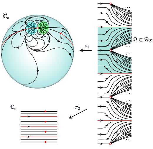
Figure 10. The Riemann surface ${\mathcal{R}}_{X}$ and a fundamental domain $\Omega$ in the universal cover of ${\widehat{\mathbb{C}}}_{z}\backslash\mathcal{S}_{X}$ for the vector field $X(z)=z{\text{\myfont e}}^{z}\frac{\partial}{\partial z}$.

Remark 5.9.

Let $X$ be a singular complex analytic vector field on the Riemann sphere with an essential singularity at $\infty\in{\widehat{\mathbb{C}}}_{z}$. A fundamental region $\Omega$ is the universal cover of ${\mathbb{C}}_{z}\backslash\mathcal{Z}$ if and only if all the zeros of $X$ and the essential singularity at $\infty$ have zero residues.

Example 5.2 (Two direct non logarithmic singularities over $\infty$).

The vector field

$X(z)=\tan(z)\frac{\partial}{\partial z}$

has a multivalued

$\Psi_{X}(z)=\int^{z}\cot(\zeta)d\zeta=\log(\sin(z))+c$,

see Figure 5.d. Its critical points are $\{(2k+1)\pi/2\ |\ k\in{\mathbb{Z}}\}$, corresponding to the poles of $X(z)$, with critical values, of the principal branch, $\{0,i\pi\}$. However, because of the multivalued nature of $\Psi_{X}$, the 1–form $\omega_{X}$ has residue 1 at $\{\ell\pi\ |\ \ell\in{\mathbb{Z}}\}$, which are the zeros of $X$. In fact $\Psi_{X}(z)$ has critical values $\{2\pi\ell i,2\pi\ell\ |\ \ell\in{\mathbb{Z}}\}$. On the other hand, the only asymptotic value that $\Psi_{X}$ has is $\infty\in{\widehat{\mathbb{C}}}_{t}$, i.e. it has no finite asymptotic values. The asymptotic value $\infty$ is not isolated. The accurate study of its multiplicity is the goal of a future project.

5.3. Localizing incomplete trajectories

As motivation for the study of the incomplete trajectories at an essential singularity, first recall that the separatrices of poles $p$ of $X$ are incomplete trajectories. Moreover, poles $p$ of $X$ correspond to algebraic singularities of $\Psi^{-1}_{X}$, in particular to critical points of $\Psi_{X}$ with the corresponding critical value $\widetilde{p}=\Psi_{X}(p)\in{\mathbb{C}}_{t}$. This can be summarized as the following.

Remark 5.10.

Let $X$ be a singular complex analytic vector field on the Riemann sphere with a pole at $p\in{\widehat{\mathbb{C}}}_{z}$.

There exists an incomplete trajectory $z(\tau)$ of $X$ having $\alpha$ or $\omega$–limit at $p$ if and only if there exists a finite critical value $\widetilde{p}\in{\mathbb{C}}_{t}$ of $\Psi_{X}$.

Moreover, the separatrices $\alpha_{\widetilde{p}}(\tau)\subset{\widehat{\mathbb{C}}}_{z}$ of the pole $p$ are the incomplete trajectories $z(\tau)$ alluded to above. They satisfy

$\lim\limits_{\tau\to\infty}\Psi_{X}(\alpha_{\widetilde{p}}(\tau))=\widetilde{p}$.

With this in mind, the following is straightforward.

Lemma 5.11.

Let $X$ be a singular complex analytic vector field on $M$ with an essential singularity at $e\in M$. There exists an incomplete trajectory $z(\tau)$ of $X$ having $\alpha$ or $\omega$–limit at $e\in M$ if and only if there exists a finite asymptotic value $a\in{\mathbb{C}}_{t}$ of $\Psi_{X}$, whose asymptotic path $\alpha_{a}(\tau)$ is a trajectory of $X$.

Proof.

The argument follows directly from the definitions of asymptotic path of a finite asymptotic value of $\Psi_{X}$ and of incomplete trajectories of $X$. ∎

Remark 5.12.

Lemma 5.11 is independent of whether $\Psi_{X}$ is single or multivalued. In fact when $\Psi_{X}$ is multivalued, the upshot is that there will be an infinite number of said trajectories, as in Example 5.1.

Theorem 1.3 (Finite asymptotic values and incomplete trajectories).

Let $X$ be a singular complex analytic vector field on $M$ with an essential singularity at $e\in M$.

1. Any neighborhood $U_{a}(\rho)$ of a transcendental singularity $U_{a}$ of $\Psi_{X}^{-1}$ over a finite asymptotic value $a\in{\mathbb{C}}_{t}$, contains an infinite number of incomplete trajectories of $X$.

2. If $\Psi_{X}$ has no finite asymptotic values, then $X$ has an infinite number of poles accumulating at $e\in M$.

Proof.

For statement (1), first consider the case when $U_{a}$ is a logarithmic singularity of $\Psi_{X}^{-1}$. Recalling Proposition 3.10.1, note that for $\rho>0$ small enough, the neighborhood $U_{a}(\rho)$ of a logarithmic singularity $U_{a}$ over a finite asymptotic value $a$ is a hyperbolic tract. It consists of an infinite number of hyperbolic sectors, and the separatrices of each hyperbolic sector are incomplete trajectories. Thus any neighborhood $U_{a}(\rho)$ of the logarithmic singularity $U_{a}$ contains an infinite number of incomplete trajectories.

On the other hand, if the transcendental singularity $U_{a}$ of $\Psi_{X}^{-1}$ is non logarithmic, Theorem (Isolated singular values) tells us that the finite asymptotic value $a$ is non isolated. Hence there are an infinite number of finite singular values (bounded by $\left\lvert a\right\rvert+\varepsilon$ for $\varepsilon>0$), say $\{a_{\sigma}\}$.

Moreover, by Theorem 1.1, $U_{a}$ is non separate. Thus for any $\rho_{a}>0$, the neighborhood $U_{a}(\rho_{a})$ contains an infinite number of neighborhoods $U_{a_{\sigma}}(\rho_{\sigma})$, for appropriate $\{\rho_{\sigma}>0\}$. Without loss of generality, assume that the collection $\{a_{\sigma}\}$ is precisely those $a_{\sigma}$ which satisfy

(20) $$U_{a_{\sigma}}(\rho_{\sigma})\subset U_{a}(\rho_{a}).$$

If an infinite number of the $a_{\sigma}$ are critical values, we are done: these critical values have corresponding critical points that are poles of $X$. Thus, by (20), any neighborhood $U_{a}(\rho)$ of the non logarithmic singularity $U_{a}$ contains an infinite number of incomplete trajectories.

Otherwise the collection $\{a_{\sigma}\}$ contains an infinite number of distinct (finite) asymptotic values. Without loss of generality, we shall assume that the $\{a_{\sigma}\}$ are all asymptotic values and that they once again satisfy (20). Now, recall that the associated Riemann surface ${\mathcal{R}}_{X}$ has as its (ideal) boundary precisely the branch points corresponding to all the asymptotic values of $\Psi_{X}$.

Since the (ideal) boundary of ${\mathcal{R}}_{X}$ is totally disconnected, then every single branch point corresponding to the singularities $U_{a_{\sigma}}$ has a trajectory $\widetilde{\alpha}_{\sigma}(\tau)\subset{\mathcal{R}}_{X}$ arriving to it. This trajectory projects downwards, via $\pi_{1}$, to an incomplete trajectory $\alpha_{\sigma}(\tau)\subset U_{a_{\sigma}}(\rho_{\sigma})\subset U_{a}(\rho_{a})$.

The proof of statement (2) is by contradiction. Assume that there is only a finite number of poles of $X$, the number of incomplete trajectories is then finite. This contradicts Theorem 1.2. ∎

The interested reader can compare the above results with theorems 1.2 and 1.3 of [36].

Remark 5.13.

Whenever there is an essential singularity of $X$, we have the dichotomy described below.

$\mathchoice{\mathbin{\vbox{\hbox{\scalebox{0.5}{$\displaystyle\bullet$}}}}}{\mathbin{\vbox{\hbox{\scalebox{0.5}{$\textstyle\bullet$}}}}}{\mathbin{\vbox{\hbox{\scalebox{0.5}{$\scriptstyle\bullet$}}}}}{\mathbin{\vbox{\hbox{\scalebox{0.5}{$\scriptscriptstyle\bullet$}}}}}$ If $\Psi_{X}$ has no finite asymptotic values, then $X$ has an infinite number of poles accumulating at the essential singularity of $X$ at $e\in M$.

$\mathchoice{\mathbin{\vbox{\hbox{\scalebox{0.5}{$\displaystyle\bullet$}}}}}{\mathbin{\vbox{\hbox{\scalebox{0.5}{$\textstyle\bullet$}}}}}{\mathbin{\vbox{\hbox{\scalebox{0.5}{$\scriptstyle\bullet$}}}}}{\mathbin{\vbox{\hbox{\scalebox{0.5}{$\scriptscriptstyle\bullet$}}}}}$ If $X$ only has a finite number of poles, then $\Psi_{X}$ has (at least) one finite asymptotic value.

5.4. What can be said about $X$ without an explicit knowledge of $\Psi_{X}$?

Sometimes the global flow box $\Psi_{X}$ is in non closed form, however the knowledge of $X$ is enough for a variety of applications. As a direct consequence of Theorem 1.3, we have the following result, which clearly extends Langley’s result in [28].

Corollary 5.14.

Let $X=f(z)\frac{\partial}{\partial z}$ be a singular complex analytic vector field on $M$ with an essential singularity at $e\in M$. Any neighborhood $U_{\widetilde{a}}(\rho)$ of a transcendental singularity $U_{\widetilde{a}}$ of $f^{-1}$ over a non zero asymptotic value $\widetilde{a}\in{\widehat{\mathbb{C}}}_{t}\backslash\{0\}$ contains an infinite number of incomplete trajectories of $X$.

Proof.

By definition, $f:M\longrightarrow{\widehat{\mathbb{C}}}_{t}$ is transcendental meromorphic. Since $f$ has a non zero asymptotic value $\widetilde{a}$, it then follows that there is an asymptotic path $\widetilde{\alpha}(\tau)$ of $f$ such that $\left\lvert\frac{1}{f(\widetilde{\alpha}(\tau))}\right\rvert\subset D\Big{(}\frac{1}{\left\lvert\widetilde{a}\right\rvert},\varepsilon\Big{)}$ for small enough $\varepsilon>0$ and large enough $\tau>0$. Thus,

$\lim\limits_{\tau\to\infty}\Psi_{X}\big{(}\widetilde{\alpha}(\tau)\big{)}=a\in{\mathbb{C}}_{t}$,

i.e. $\Psi_{X}$ has $a$ as a finite asymptotic value. By Theorem 1.3, we are done. ∎

The relationship between the singularities of $f^{-1}$ and $\Psi_{X}^{-1}$ is a priori unknown. For the simplest kind, however we have the following correspondence.

Lemma 5.15.

The following assertions are equivalent.

1. $f^{-1}$ has a logarithmic singularity over an asymptotic value $\widetilde{a}\in{\widehat{\mathbb{C}}}$.

2. $\Psi_{X}^{-1}$ has a logarithmic singularity over the corresponding asymptotic value $a\in{\widehat{\mathbb{C}}}$ as in (7).

Proof.

$(1)\Rightarrow(2)$. From the definition, a transcendental singularity $U$ is a logarithmic singularity over $\widetilde{a}$ if $f:U(\rho)\longrightarrow D(\widetilde{a},\rho)\backslash\{\widetilde{a}\}\subset{\widehat{\mathbb{C}}}$ is a universal covering for some $\rho>0$. Hence, there exists a biholomorphism $\phi:D(0,r)\longrightarrow U(\rho)$ such that $f(\phi(w))=\exp(w)$ for small enough $r>0$. In other words, $\Psi_{X}^{-1}$ has a logarithmic singularity over $a$.

$(1)\Leftarrow(2)$. Since $\Psi_{X}$ is a universal cover, locally $\Psi_{X}(\phi(w))=\exp(w)$ so $f(\psi(w))=\frac{d}{dw}\exp(w)=\exp(w)$, i.e. $f$ is a universal covering for some $\rho>0$. ∎

Lemma 5.15 together with Theorem 1.1 and Proposition 3.10 immediately provide us with the following result, which complements Corollary 5.14. Once again compare this with [28] theorem 1.2.

Proposition 5.16.

Let $f:M\longrightarrow{\widehat{\mathbb{C}}}_{t}$ be a transcendental meromorphic function, such that $f^{-1}$ has a logarithmic singularity $U_{\widetilde{a}_{\sigma}}$ over $\widetilde{a}_{\sigma}\in{\widehat{\mathbb{C}}}_{t}$.

1. If the singularity $U_{\widetilde{a}}$ of $f^{-1}$ is over a non zero asymptotic value $\widetilde{a}\in{\mathbb{C}}^{*}\cup\{\infty\}$, then $X$, at $e\in M$, has an infinite number of hyperbolic sectors and an infinite number of incomplete trajectories.

2. If the singularity $U_{\widetilde{a}}$ of $f^{-1}$ is over the asymptotic value $0=\widetilde{a}\in{\mathbb{C}}_{t}$, then $X$ at $e\in M$ has an infinite number of elliptic sectors.

Proof.

Because of Lemma 5.15, it follows that $\Psi_{X}^{-1}$ has a logarithmic singularity over $a$, recall Equation (7). By Theorem 1.1, $f$ has at most a finite number of zeros and poles in the exponential tract. Thus

$$\lim\limits_{\tau\to\infty}\Psi_{X}\big{(}\widetilde{\alpha}(\tau)\big{)}=\begin{cases}a\in{\mathbb{C}}_{t}&\text{if }\widetilde{a}\in{\mathbb{C}}^{*}\cup\{\infty\},\\ a=\infty&\text{if }\widetilde{a}=0,\end{cases}$$

and hence by Proposition 3.10 we are done. ∎

6. Decomposition in ${\mathfrak{Re}\left(X\right)}$–invariant regions by removing incomplete trajectories

Here we consider singular complex analytic vector fields $X$ with a finite number of essential singularities, on compact Riemann surfaces $M_{\mathfrak{g}}$ of genus $\mathfrak{g}\geq 0$. Its singular complex analytic global flow box map is

$\Psi_{X}:M_{\mathfrak{g}}\backslash\mathcal{S}_{X}\longrightarrow{\widehat{\mathbb{C}}}_{t}$.

We present a natural decomposition of $M_{\mathfrak{g}}$, under the flow of ${\mathfrak{Re}\left(X\right)}$, in the spirit of A. A. Andronov et al. [5] (for differential equations) and K. Strebel [39] (for quadratic differentials). We recall the following phenomena.

Example 6.1 (Meromorphic vector fields with one recurrence region).

The constant vector fields on a torus ${\mathbb{C}}/\Lambda$ having ${\mathfrak{Re}\left(X\right)}$ with irrational vector fields are the simplest holomorphic vector fields with recurrence region, the whole ${\mathbb{C}}/\Lambda$. When $\mathfrak{g}\geq 2$, every compact Riemann surface $N_{\mathfrak{g}}$ has meromorphic vector fields $X$ with only poles, equivalent to holomorphic $1$–forms $\omega_{X}$. Moreover, by a classical result of S. Kerchoff et al. [26], almost every rotation ${\mathfrak{Re}\left({\text{\myfont e}}^{i\theta}X\right)}$ has a dense trajectory. We have that the closure of a recurrent trajectory which is the whole $N_{\mathfrak{g}}$. In fact, $(N_{\mathfrak{g}},{\text{\myfont e}}^{i\theta}X)$ is without boundary components.

Performing a suitable surgery in the above, as seen in [31] for further details, we can obtain Riemann surfaces $\overline{N}$ of genus $\mathfrak{g}\geq 1$, with ${\tt h}\geq 1$ boundary components, and where ${\mathfrak{Re}\left({\text{\myfont e}}^{i\theta}X)\right)}$ has a dense trajectory in $\overline{N}$.

Definition 6.1.

[39] 1. The open canonical regions are pairs (domain & holomorphic vector field) as follows

(21) $$\begin{array}[]{c}\begin{array}[]{rcr}\hbox{\it half plane }\mathscr{H}=\big{(}\mathbb{H}^{2},\frac{\partial}{\partial z}\big{)},&&\hbox{\it strip }\mathscr{S}=\big{(}\{0<{\mathfrak{Im}\left(z\right)}<h\},\frac{\partial}{\partial z}\big{)},\\ &&\vspace{-.2cm}\hfil\\ \hbox{\it half cylinder }\mathscr{C}=\big{(}\Delta_{1},\frac{2\pi iz}{r}\frac{\partial}{\partial z}\big{)},&&\hbox{\it annulus }\mathscr{A}=\big{(}\Delta_{R}\backslash\overline{\Delta}_{1},\frac{2\pi iz}{r}\frac{\partial}{\partial z}\big{)},\\ &&\vspace{-.3cm}\hfil\end{array}\\ \hbox{\it recurrence }\mathscr{R}=\big{(}N,{\text{\myfont e}}^{i\theta}X\big{)}.\end{array}$$

Here $\mathbb{H}^{2}=\{{\mathfrak{Im}\left(z\right)}>0\}$ is the open half plane; $\Delta_{R}=\{|z|<R\}$ is an open disk; $h,\,r\in{\mathbb{R}}^{+}$ are parameters; and $N$ is the interior of $\overline{N}$ of genus $\mathfrak{g}\geq 1$, with ${\tt h}\geq 1$ boundary components, where ${\mathfrak{Re}\left({\text{\myfont e}}^{i\theta}X)\right)}$ has a dense trajectory in $\overline{N}$.

2. Given $(M,X)$, a pair $(\mathcal{U},X)$ is a canonical region of $X$ when it is holomorphically equivalent to one element in (21) and it is maximal.

By recalling Diagram 5, the canonical regions in (21) have flat metrics $(\mathcal{U},g_{X})$ and geodesic boundaries. As a valuable tool for the construction of vector fields, surgery tools are widely used, v.g. [39] p.  56 “welding of surfaces”, [31], or [42] §3.2.–3.3 for general discussion.

Corollary 6.2 (Isometric glueing).

Let $(\mathcal{U}_{1},g_{X})$, $(\mathcal{U}_{2},g_{Y})$ be two flat surfaces arising from two singular complex analytic vector fields $X$ and $Y$. Assume that both spaces $\mathcal{U}_{1},\,\mathcal{U}_{2}$ have as geodesic boundary components of the same length, the trajectories $\sigma_{1}(\tau)$, $\sigma_{2}(\tau)$ of ${\mathfrak{Re}\left(X\right)}$ and ${\mathfrak{Re}\left(Y\right)}$, $\tau\in I\subset{\mathbb{R}}$. The isometric glueing of them along these geodesic boundary is well defined and provides a new flat surface on $\mathcal{U}_{1}\cup\mathcal{U}_{2}$ arising from a new complex analytic vector field. $\Box$

There are several ways to construct vector fields on any $M_{\mathfrak{g}}$.

Example 6.2.

Let $({\widehat{\mathbb{C}}}_{z},X)$ be a singular complex analytic vector field with essential singularities. Since any $M_{\mathfrak{g}}$ allows non constant meromorphic functions $h$, $Y=(h\circ\Psi_{X})^{*}\frac{\partial}{\partial t}$ is then a singular complex analytic vector field with essential singularities on $M_{\mathfrak{g}}$.

Example 6.3 (Families of vector fields $(M_{\mathfrak{g}},X)$, $\mathfrak{g}\geq 1$, with the simplest essential singularity).

Let $({\widehat{\mathbb{C}}},{\text{\myfont e}}^{z}\frac{\partial}{\partial z})$ and $(N_{\mathfrak{g}},Y)$ be vector fields, where $Y$ is a meromorphic vector field such that $\omega_{X}$ is holomorphic. We perform the isometric glueing

$(M_{\mathfrak{g}},X)=\big{(}{\widehat{\mathbb{C}}},g_{{\text{\myfont e}}^{z}\frac{\partial}{\partial z}}\big{)}\cup(N,g_{Y})$.

By construction $X$ has a unique isolated essential singularity $e\in M_{\mathfrak{g}}$ with two entire sectors $\mathscr{E}\mathscr{E}$ as ${\text{\myfont e}}^{z}\frac{\partial}{\partial z}$. Firstly, $\Psi_{X}$ has an infinite number of finite asymptotic values $\{0+\sum_{j=1}^{2\mathfrak{g}}{\mathbb{Z}}\Pi_{j}\}$, where $0$ is the unique finite asymptotic value of $\Psi_{W}$ and $\{\Pi_{j}\}$ are the $2\mathfrak{g}$ periods of $\omega_{Y}$. In particular, for $\mathfrak{g}\geq 2$, the finite asymptotic values of $\Psi_{X}$ are a dense set in ${\mathbb{C}}_{t}$.

Secondly, since a non constant meromorphic map $h:M_{\mathfrak{g}}\longmapsto{\widehat{\mathbb{C}}}$ has degree $d\geq 2$, we can observe that $X$ is different from $(h\circ\Psi_{Z})^{*}\frac{\partial}{\partial t}$, for any $h$ and any a singular complex analytic vector field $Z$ on the Riemann sphere with global flow box $\Psi_{Z}$. By contradiction, assume $X=(h\circ\Psi_{Z})^{*}\frac{\partial}{\partial t}$. If $e\in M_{\mathfrak{g}}$ is a non ramified point of $h$, then necessarily $h(e)$ is an essential singularity of $Z$, hence $X=h^{*}Z$ has $2\leq d^{\prime}\leq d$ essential singularities, which is a contradiction. If $e$ is a branch point of $h$, then $h(e)$ is an essential singularity of $Z$ with necessarily only one sector $\mathscr{E}$. This is topologically impossible.

Proposition 6.3.

Let $\Psi_{X}:{\mathbb{C}}_{z}\longrightarrow{\widehat{\mathbb{C}}}_{t}$ be a singular complex analytic function.

1. The following assertions are equivalent.

   i. $\Psi_{X}$ is single valued.

   ii. The pair $({\mathbb{C}}_{z},X)$ can be constructed by isometric glueing of half planes and strips, as in (21).

2. Furthermore, if all the finite singular values of $\Psi_{X}$ are in a line $\{{\mathfrak{Im}\left(t\right)}=cte\}$, then the pair $({\mathbb{C}}_{z},X)$ can be constructed by isometric glueing of half planes. $\Box$

Assertion (2) in the rational case, is related to beautiful problems, see [11], [12]. In the other direction, we assume the knowledge of the vector field as follows.

Proposition 6.4 (Decomposition for singular complex analytic vector fields).

Let $M$ be an arbitrary connected Riemann surface.

1. Let $X$ be a singular complex analytic vector field on $M$, having at most a locally finite set of real incomplete trajectories $\{z_{\vartheta}(\tau)\}$. Therefore, $X$ admits a locally finite decomposition in half planes, strips, cylinders and annulus as above.

2. Conversely, assume that $M$ is obtained by the paste of a finite or infinite number of closures of canonical regions in (21), there then exists a singular complex analytic vector field $X$ on $M$, extending the vector fields of the canonical regions.

3. Assume that the resulting $M_{\mathfrak{g}}$ is compact. The decomposition is finite if and only if $X$ is meromorphic. Moreover, the decomposition is infinite if and only if $X$ has at least one essential singularity.

Proof.

For assertion 1, consider a complete trajectory $\{z_{0}(\tau)\}\subset M$ of ${\mathfrak{Re}\left(X\right)}$. It is an embedding of ${\mathbb{R}}$ or a circle in $M$. If we can move $\{z_{0}(\tau)\}$, with the real flow of ${\mathfrak{Im}\left(X\right)}$ in $M\backslash\cup_{\vartheta}\{z_{\vartheta}(\tau)\}$, this produces a tubular neighborhood of it. The maximal tubular neighborhood correspond to half planes, strips, half cylinders or annulus. On the other hand, if we can move $\{z_{0}(\tau)\}$ with the real flow of ${\mathfrak{Im}\left(X\right)}$ in $M\backslash\cup_{\vartheta}\{z_{\vartheta}(\tau)\}$, then necessarily $\{z_{0}(\tau)\}$ is a copy of ${\mathbb{R}}$ and its closure in $M$ corresponds to a recurrence region $\overline{\mathcal{R}}$.

Assertion 2 is immediate from Lemma 2.8.

Assertion 3 follows from Theorem 1.2. ∎

7. Summary and future directions

We emphasize the natural properties that come from our study. Theorem 1.1 provides the following classification of transcendental singularities of $\Psi_{X}^{-1}$.

$U_{a}$ is separate $\Leftrightarrow U_{a}$ is logarithmic $\begin{cases}U_{a}(\rho)\text{ is a hyperbolic tract when }a\in{\mathbb{C}}_{t},\\ U_{a}(\rho)\text{ is an elliptic tract when }a=\infty.\end{cases}$

$U_{a}$ is non separate $\Leftrightarrow U_{a}(\rho)$ contains an infinite number of singularities of $\Psi_{X}^{-1}$.

Note that the neighborhoods $U_{a}(\rho)$, on the right hand side, describe the geometry of the vector field on $M$

In addition, non separate transcendental singularities originate the following cases.

$\begin{cases}U_{a}(\rho)\text{ contains only algebraic singularities, see Example \ref{Ejemplo-ExpSinExp}},\\ U_{a}(\rho)\text{ contains only transcendental singularities, see Example \ref{Ejemplo-IntExpExp}},\\ U_{a}(\rho)\text{ contains algebraic and transcendental singularities, see Example \ref{Ejemplo-ExpSin-z}}.\end{cases}$

Iversen’s classification is related to the one described by Theorem 1.1 as follows.

Table 2. Relationship between Iversen’s classification and separate/non separate

	Separate	Non separate
Direct	Logarithmic	$\checkmark$
Indirect	$\times$	$\checkmark$

An accurate examination of the multivalued case for $\Psi_{X}$ remains as a future project.

References

- [1] L. V. Ahlfors, Conformal Invariants Topics in Geometric Function Theory, McGraw–Hill, New York, 1973.
- [2] A. Alvarez–Parrilla, J. Muciño–Raymundo, Dynamics of singular complex analytic vector fields with essential singularities I, Conform. Geom. Dyn. 21 (2017), 126–224. http://dx.doi.org/10.1090/ecgd/306
- [3] A. Alvarez–Parrilla, J. Muciño–Raymundo, Symmetries of complex analytic vector fields with an essential singularity on the Riemann sphere, Adv. Geom. 21, no. 4 (2021), 483–504. http://dx.doi.org/10.1515/advgeom-2021-0002
- [4] A. Alvarez–Parrilla, J. Muciño–Raymundo, Dynamics of singular complex analytic vector fields with essential singularities II, J. Singul. (2022), 1–78. https://www.journalofsing.org/volume24/article1.html
- [5] A. A. Andronov, E. A. Leontovich, I. I. Gordon, A. G. Maier, Qualitative Theory of Second–Order Dynamic Systems, J. Wiley & Sons, New–York, Toronto, 1973.
- [6] C. A. Berenstein, A. Gay, Complex Variables, 2rd ed., Springer, Berlin, 1997. https://link.springer.com/book/10.1007/978-1-4612-3024-3
- [7] W. Bergweiler, A. Eremenko, On the singularities of the inverse to a meromorphic function of finite order, Rev. Mat. Iberoamericana 11, 2 (1995), 355–373. http://dx.doi.org/10.4171/RMI/176
- [8] L. Brickman, E. S. Thomas, Conformal equivalence of analytic flows, J. Differential Equations 25, 3 (1977), 310–324. https://core.ac.uk/download/pdf/82638812.pdf
- [9] R. L. Devaney, Complex exponential dynamics, in Handbook of Dynamical Systems, H. W. Broer et al. eds., North Holland, Amsterdam (2010), 125–223. https://www.sciencedirect.com/handbook/handbook-of-dynamical-systems/vol/3/suppl/C
- [10] A. Eremenko, Singularities of inverse functions, (2021) 16 p. https://arxiv.org/abs/2110.06134
- [11] A. Eremenko, A. Gabrielov, Rational functions with real critical points and the B. and M. Shapiro conjecture in real enumerative geometry, Ann. of Math. (2) 155 (2002), no. 1, 105–129. http://dx.doi.org/10.2307/3062151
- [12] A. Eremenko, A. Gabrielov, An elementary proof of the B. and M. Shapiro conjecture for rational functions, in Notions of positivity and the geometry of polynomials, 167–178, Trends Math., Birkhäuser/Springer Basel AG, Basel, 2011. http://dx.doi.org/10.1007/978-3-0348-0142-3_10
- [13] F. Forstneric, Stein Manifolds and Holomorphic Mappings, Springer–Verlag, Berlin 2011. https://link.springer.com/book/10.1007/978-3-319-61058-0
- [14] A. Garijo, A. Gasull, X. Jarque, Normal forms for singularities of one dimensional holomorphic vector fields, Electron. J. Differential Equations 122 (2004), 7 p. https://www.emis.de/journals/EJDE/2004/122/garijo.pdf
- [15] W. Gross, Über die Singularitäten analytischer Funktionen, Mh. Math. Phys. 29, (1918), 3–47. https://doi.org/10.1007/BF01700480
- [16] A. Guillot, Complex differential equations and geometric structures in curves, in Hernández–Lamoneda L. et al. eds., Geometrical Themes Inspired by the –body Problem, 1–47, Lect. Notes Math., vol. 2204, Springer (2018). https://doi.org/10.1007/978-3-319-71428-8_1
- [17] 0. Hájek Notes on meromorphic dynamical systems I, Czechoslovak Math. J. 16, 91 (1966), 14–27.
- [18] 0. Hájek Notes on meromorphic dynamical systems II, Czechoslovak Math. J. 16, 91 (1966), 28–35.
- [19] 0. Hájek Notes on meromorphic dynamical systems III, Czechoslovak Math. J. 16, 91 (1966), 36–40.
- [20] M. Heitel, D. Lebiedz, On analytical and topological properties of separatrices in 1–D holomorphic dynamical systems and complex–time Newton flows, Preprint (2019), 19 p. https://arxiv.org/abs/1911.10963
- [21] M. E. Herring, Mapping properties of Fatou components, Ann. Acad. Sci. Fenn. Math. 23 (1998), 263–274. https://www.acadsci.fi/mathematica/Vol23/herring.pdf
- [22] E. Hille, On the zeros of the functions of the parabolic cylinder, Arkiv für Mathematik, Astronomy Och Physik 18, 26 (1924), 1–56.
- [23] K. Hockett, S. Ramamurti, Dynamics near the essential singularity of a class of entire vector fields, Trans. Amer. Math. Soc. 345, 2 (1994), 693–703. https://doi.org/10.1090/S0002-9947-1994-1270665-5
- [24] F. Iversen, Recherches sur les fonctions inverses des fontions méromorphes, Ph. D. Thesis, Helsingfords (1914). https://catalog.hathitrust.org/Record/007896919
- [25] J. Jenkins, Univalent Functions and Conformal Mapping, Ergebnisse Der Mathematik Und Iher Grenzgebiete, Springer–Verlag, Berlin, 1958. https://doi.org/10.1007/978-3-642-88563-1
- [26] S. Kerchoff, H. Masur, J. Smillie, Ergodicity of billiards flows and quadratic differentials, Ann. of Math. 2, 134 (1986), 293–311. https://doi.org/10.2307/1971280
- [27] S. Kobayashi, Transformation Groups in Differential Geometry, Springer–Verlag, Berlin, 1972. https://doi.org/10.1007/978-3-642-61981-6
- [28] J. K. Langley, Trajectories escaping to infinity in finite time, Procc. Amer. Math. Soc. 145, 5, May (2017), 2107–2117. https://dx.doi.org/10.1090/proc/13377
- [29] J. K. Langley, Transcendental singularities for meromorphic functions with logarithmic derivative of finite lower order, Comput. Methods Funct. Theory 19 (2019), 117–133. https://doi.org/10.1007/s40315-018-0253-3
- [30] J. L. López, J. Muciño–Raymundo, On the problem of deciding whether a holomorphic vector field is complete, in Complex analysis and related topics (Cuernavaca, 1996) 171–195, Ramírez de Arellano et al. eds., Oper. Theory Adv. Appl. 114, Birkhäuser, Basel, (2000), https://doi.org/10.1007/978-3-0348-8698-7_13
- [31] J. Muciño–Raymundo, Complex structures adapted to smooth vector fields, Math. Ann. 322 (2002), 229–265. https://doi.org/10.1007/s002080100206
- [32] D. J. Needham, A. C. King, On meromorphic complex differential equations, Dynam. Stability Systems 9, 2 (1994), 99–122. https://doi.org/10.1080/02681119408806171
- [33] R. Nevanlinna, Analytic Functions, Springer–Verlag, 1970. https://doi.org/10.1007/978-3-642-85590-0
- [34] I. Richards, On the classification of noncompact surfaces, Trans. Amer. Math. Soc. 106 (1963), 259–269. https://doi-org/10.1090/S0002-9947-1963-0143186-0
- [35] S. L. Segal, Nine Introductions to Complex Analysis, Rev. Ed., North–Holland, Amsterdam, 2008.
- [36] D. J. Sixsmith, A new characterization of the Eremenko–Lyubich class, J. Anal. Math. 123 (2014), 95–105. https://doi.org/10.1007/s11854-014-0014-9
- [37] A. Speiser, Über Riemannsche Flächen, Comment. Math. Helv. 2 (1930), 284–293.
- [38] N. Steinmetz, Nevanlinna Theory, Normal Families and Algebraic Differential Equations, Springer, 2017. https://doi.org/10.1007/978-3-319-59800-0
- [39] K. Strebel, Quadratic Differentials, Springer–Verlag, Berlin, 1984. https://doi.org/10.1007/978-3-662-02414-0
- [40] M. Taniguchi, Explicit representations of structurally finite entire functions, Proc. Japan Acad. Ser. A Math. Sci. 77 (2001), 68–70. https://projecteuclid.org/euclid.pja/1148393085
- [41] M. Taniguchi, Synthetic deformation space of an entire function, Contemp. Math. 303 (2002), 107–136. http://dx.doi.org/10.1090/conm/303/05238
- [42] W. P. Thurston, Three–Dimensional Geometry and Topology. Vol. 1., Princeton University Press, Princeton NJ, 1997.
- [43] J. Zheng, Value Distribution of Meromorphic Functions, Tsinghua Univ. Press, Springer, Heidelberg, 2010. https://link.springer.com/book/10.1007/978-3-642-12909-4