Learning in Feedback-driven Recurrent Spiking Neural Networks using full-FORCE Training

Abstract

Feedback-driven recurrent spiking neural networks (RSNNs) are powerful computational models that can mimic dynamic systems. However, the presence of a feedback loop from the readout to the recurrent layer de-stabilizes the learning mechanism and prevents it from converging. Here, we propose a supervised training procedure for RSNNs, where a second network is introduced only during the training, to provide hint for the target dynamics. The proposed training procedure consists of generating targets for both recurrent and readout layers (i.e., for a full RSNN system). It uses the recursive least square-based First-Order and Reduced Control Error (FORCE) algorithm to fit the activity of each layer to its target. The proposed full-FORCE training procedure reduces the amount of modifications needed to keep the error between the output and target close to zero. These modifications control the feedback loop, which causes the training to converge. We demonstrate the improved performance and noise robustness of the proposed full-FORCE training procedure to model 8 dynamical systems using RSNNs with leaky integrate and fire (LIF) neurons and rate coding. For energy-efficient hardware implementation, an alternative time-to-first-spike (TTFS) coding is implemented for the full-FORCE training procedure. Compared to rate coding, full-FORCE with TTFS coding generates fewer spikes and facilitates faster convergence to the target dynamics.

I Introduction

Spiking Neural Networks (SNNs) are biologically-realistic computational models that exploit the dynamics of the central nervous system in primates [1]. SNNs facilitate energy-efficient VLSI implementation on an event-driven neuromorphic hardware platform such as DYNAPs [2], $\mu$Brain [3], and Loihi [4]. Recurrent spiking neural networks (RSNNs) are a type of SNNs that can accurately mimic a dynamical system [5], where mimicking involves modeling the interaction of system components over time and performing analogous tasks when inputs are silent over thousands of time steps [6].

Reservoir computing is an important example of RSNNs [7, 8, 9]. It consists of an input layer, a reservoir layer of recurrently-connected neurons, and an output readout layer (see Figure 1). The reservoir may receive feedback from the readout layer [10]. Training a reservoir computing system is challenging for three reasons [11, 12, 13]. First, the feedback loop can prevent the training to converge. This is due to the delayed effect from the feedback signal, which can cause the output to diverge away from the target response [14]. Second, it suffers from the credit assignment problem of identifying which neurons and synapses have the highest impact on the output [15]. Finally, RSNNs that have spontaneous chaotic activity, i.e., systems that are active without any input in the pre-training phase are difficult to train [16, 17, 18, 19].

To address these limitations, prior learning approaches have introduced several simplifications such as 1) eliminating the feedback loop, 2) training only the synaptic connections between the reservoir and readout, and 3) suppressing chaotic activity in the pre-training phase. The Liquid State Machine (LSM) is one such reservoir computing system with the aforementioned simplifications [20, 21, 22].

Some recent efforts have addressed the training of feedback-driven RSNNs that may include spontaneous chaotic activity in the pre-training phase. In [23], backpropagation through time (BPTT) is proposed for SNNs, which is extended in [24, 25, 26] to train both the reservoir and readout of an LSM. In these approaches, the reservoir is trained using an unsupervised algorithm such as spike timing dependent plasticity (STDP) [27], while the readout is trained using BPTT. Following are its limitations. First, BPTT requires unfolding an RSNN into effective network layers, one for each time stamp and obtaining gradient over the time period. This leads to an exponential increase in the computational complexity [24]. Second, BPTT suffers from the vanishing gradient problem, where certain components of the gradient computed on the loss function may get close to zero [28]. Vanishing gradients stall parameter updates during the training.

In [29], a recursive least square-based First-Order and Reduced Control Error (FORCE) algorithm is proposed to train the readout layer of an RSNN with a feedback signal from the readout to the spiking neurons in the reservoir. Contrary to conventional training procedures, where weight modifications are performed to reduce large errors in the output, objective of the FORCE training procedure is to reduce the amount of modifications needed to keep the error small. Such modifications are then used to control the feedback signal without needing any additional training mechanisms for the feedback loop. FORCE training procedure can train networks that exhibit chaotic activity in the pre-training phase. However, FORCE training suffers from the following limitations. First, FORCE can only model dynamical systems that can be represented using a closed-form differential equation [17]. However, there are many practical systems where such closed-form representation is difficult to obtain [30]. Second, FORCE training procedure is susceptible to input noise [31]. This is because FORCE trains only the readout and not the reservoir. Therefore, noise introduces a small variation in the response of the reservoir neurons, which triggers a domino effect using the feedback loop and eventually, diverging the output significantly from the target.

A recent training procedure, called full-FORCE can address the aforementioned limitations[32]. Here, a second recurrent network is introduced only during training to obtain targets for the reservoir neurons. It uses the FORCE algorithm to fit the response of each layer (recurrent and readout) to its target response. However, full-FORCE training requires sigmoid neurons, which are not supported on event-driven neuromorphic hardware platforms. Table I summarizes these existing training procedures.

TABLE I: Training procedures for Feedback-driven RSNNs.

	Feedback-driven RSNNs
	Feedback Driven	Training Procedure	Spontaneous Activity	LIF Neuron	Neuromorphic Computing
[20]	$\times$	Readout Only (supervised)	$\times$	$\surd$	$\surd$
[24]	$\times$	Reservoir and Readout (BPTT)	$\times$	$\surd$	$\times$
[17]	$\surd$	Readout (FORCE)	$\surd$	$\times$	$\times$
[32]	$\surd$	Reservoir and Readout (full-FORCE)	$\surd$	$\times$	$\times$
[29]	$\surd$	Readout (FORCE)	$\surd$	$\surd$	$\times$
ours	$\surd$	Reservoir and Readout (full-FORCE)	$\surd$	$\surd$	$\surd$

We propose a full-FORCE implementation for feedback-driven RSNNs using the leaky integrate and fire (LIF) neurons. We make the following key contributions.

• We implement the full-FORCE algorithm for rate coding and explore the design space of network architecture for faster convergence to the target and facilitate energy-efficient neuromorphic implementation.

• By training both reservoir and the readout layers, we illustrate the stability of the training procedure to noise.

• We provide an alternative time-to-first-spike (TTFS) implementation of the full-FORCE training procedure. We show that full-FORCE with TTFS encoding generates fewer spikes and facilitates faster convergence to the target dynamics.

We evaluate our full-FORCE training procedure (which trains both reservoir and the readout layers) against the FORCE learning (which trains only the readout layer). Results demonstrate that our full-FORCE implementation has an average 51% lower mean square error (MSE) and it provides higher tolerance to noise. Furthermore, the proposed full-FORCE implementation with TTFS coding results in 50% fewer spikes and 40% lower convergence time.

II Preliminaries

Figure 1 shows two reservoir computing architectures [7]. Both these architectures consist of an input layer, a reservoir layer of recurrently-connected neurons, and an output readout layer. The reservoir may also receive feedback from the readout. In Figure 1a, the feedback is generated directly from the readout layer. In Figure 1b, the feedback is generated from a separate (recurrent) network, which can be trained offline.

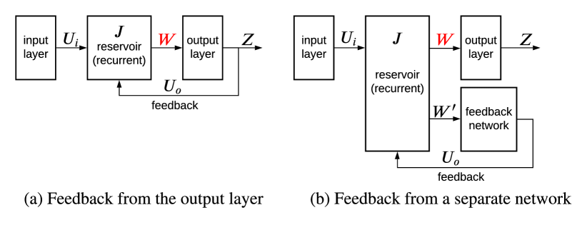
Figure 1: Different reservoir computing architectures. (a) Feedback to the recurrent reservoir is provided by the output readout units. (b) Feedback to the reservoir is provided by a separate feedback network.

II-A Difficulty in Training with Feedback Loop

Training a reservoir computing architecture with feedback is challenging. To understand this, we observe that there are two pathways in this architecture. The direct pathway is from the reservoir to the readout layer, while the feedback pathway is from the readout to the reservoir layer. Considering only the direct pathway, it is straightforward to optimize the weights $W$ such that the output $Z(t)$ is close to the target response of a dynamical system. However, due to the delay on the feedback pathway, the effect of weight updates on the output $Z(t)$ arrives at the reservoir with a time lag. Training the weights via the direct pathway reduces the output error. However, the delayed feedback from the readout causes the output $Z$ to deviate away from the target, increasing the error.

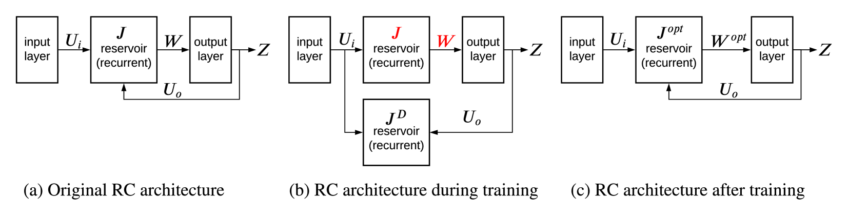
Figure 2: Learning in reservoir computing (RC) architecture using the full-FORCE training. (a) Original RC architecture. (b) Training an RC architecture using a separate target network. (c) A fully trained RC architecture.

II-B Training the Readout using FORCE

To introduce the FORCE training procedure, we focus on the architecture of Figure 1a, which can then be generalized to Figure 1b. We elaborate the training procedure considering sigmoidal neurons (see Section III for RSNNs).

Let the architecture of Figure 1a be designed to model a dynamical system whose response at time $t$ is $f(t)$. We introduce the following notations.

$$f(t)=$$ Input and target

$$U_{i}=$$ Synaptic weights between input and reservoir.

$$J=$$ Synaptic weights between the reservoir neurons.

$$Y(t)=$$ Output of the reservoir.

$$W(t)=$$ Synaptic weights between reservoir and readout.

$$U_{o}(t)=$$ Synaptic weights between readout and reservoir (feedback).

$$Z(t)=$$ Output of the readout.

Output of the architecture at time $t$ is

$$\footnotesize Z(t)=W^{T}(t)\cdot Y(t)$$ (1)

FORCE training procedure updates only the weight matrix $W$ such that the output is close to the target, i.e., $Z(t)=f(t)$. The output error is defined as $e(t)=Z(t)-f(t)$.

A key characteristics of the FORCE training is that it keeps the error signal small by making rapid weight updates. Let, weight updates are initiated at every $\Delta t$ time interval. Therefore, the weight update at time $t$ is based on the output evaluated at its previous time step, i.e., at time $t-\Delta t$. The output error at time $t$ before performing the weight update is

$$\footnotesize e_{-}(t)=Z(t-\Delta t)-f(t)=W^{T}(t-\Delta t)\cdot Y(t)-f(t)$$ (2)

After the weight update, the output error is

$$\footnotesize e_{+}(t)=W^{T}(t)\cdot Y(t)-f(t)$$ (3)

Goals of the FORCE training are as follows.

1. Reduce the output error during each weight update, i.e.,

   $$\footnotesize|e_{+}(t)|<|e_{-}(t)|$$ (4)

2. Converge the weight updates, i.e.,

   $$\footnotesize\lim\frac{e_{+}(t)}{e_{-}(t)}=1$$ (5)

Using the recursive least square (RLS) algorithm for FORCE training [17], the weight update is given by

$$\footnotesize W^{T}(t)=W^{T}(t-\Delta t)-e_{-}(t)\cdot P(t)\cdot Y(t),$$ (6)

where $P(t)$ is updated during each weight update according to

$$\footnotesize P(t)=P(t-\Delta t)-\frac{P(t-\Delta t)\cdot Y(t)\cdot Y^{T}(t)\cdot P(t-\Delta t)}{1+Y^{T}(t)\cdot P(t-\Delta t)\cdot Y(t)}.$$ (7)

Here, $P(0)=\frac{{I}}{\alpha}$, where ${I}$ is the identity matrix.

Limitations: Although, FORCE can train the reservoir connections $J$, the learning is shown to be unstable due to the feedback. Additionally, FORCE training is shown to work only when the connectivity amongst the reservoir neurons is sparse.

II-C Training the Reservoir and Readout using full-FORCE

Figure 2 illustrates how full-FORCE algorithm is used to train a reservoir computing architecture [32]. The original architecture is shown in Figure 2a. The dynamics of this architecture are as follows. The output $Z(t)$ is

$$\footnotesize Z(t)=W^{T}\cdot Y(t),$$ (8)

where $Y(t)=\mathcal{S}\big{(}X(t)\big{)}$ is a non-linear function that implements sigmoidal neurons in the reservoir and $X(t)$ is the neuron activation inside the reservoir. $X(t)$ is governed by the first-order ordinary differential equation (ODE)

$$\footnotesize\tau\frac{dX(t)}{dt}=-X(t)+J\cdot Y(t)+U_{i}\cdot f_{in}(t)+U_{o}\cdot Z(t),$$ (9)

where $f_{in}(t)$ is the input. Observe that instead of using $f(t)$ to represent both the input and target as in the case of the FORCE formulation (Sec. II-B), we decouple the two. This allows us to design a dynamical system that may receive a specific input (or no input at all) and generate a target that can be different from the input. This is fundamental to mimicking systems whose input-output relationship cannot be modeled using a closed-form differential equation. The training objective of full-FORCE is to optimize $W$ and $J$ such that $Z(t)=f_{out}(t)$, where $f_{out}(t)$ is the response of the dynamical system that we aim to model using the reservoir computing architecture.

The full-FORCE training procedure works as follows. A second reservoir network (called target-generating network) is introduced during training as shown in Figure 2b. This network is used to generate the target for every neuron in the original reservoir (henceforth referred to as task-performing network). The target-generating network is also a reservoir of randomly-connected recurrent neurons with fixed connections $J^{D}$. This reservoir is driven by both the input $f_{in}(t)$ and the output $Z(t)$. The rich dynamics of a randomly connected network allows to model many dynamical systems by suppressing chaos in a controlled manner using the two signals $f_{in}(t)$ and $Z(t)$.

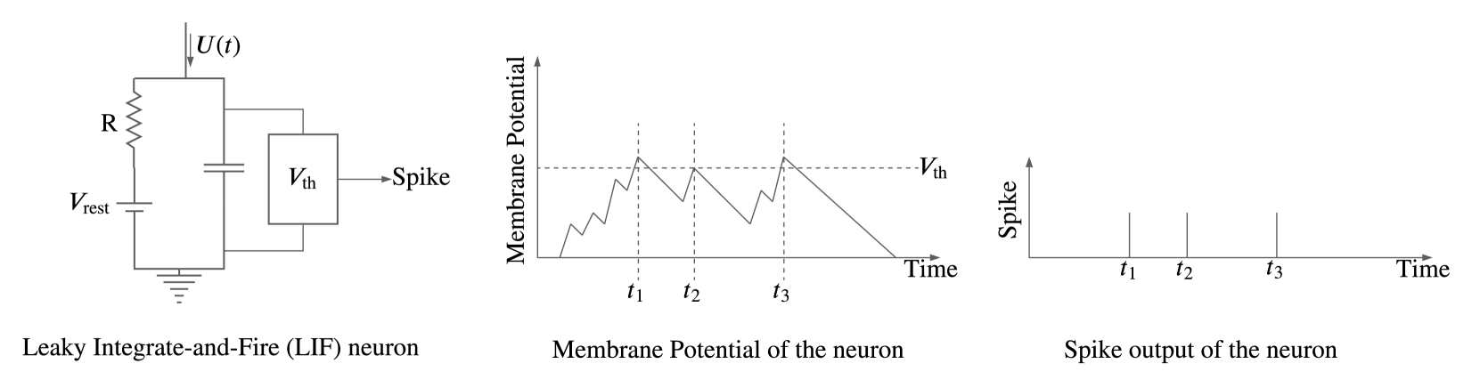
Figure 3: A leaky integrate-and-fire (LIF) neuron with current input $I(t)$ (left). The membrane potential over time of the neuron (middle). The spike output of the neuron representing its firing time (right).

During training, dynamics of the task-performing and the target-generating networks are

$$\footnotesize\tau\frac{dX(t)}{dt}=-X(t)+J\cdot Y(t)+U_{i}\cdot f_{in}(t)$$ (10)

$$\footnotesize\tau\frac{dX^{D}(t)}{dt}=-X^{D}(t)+J^{C}\cdot Y^{D}(t)+U_{i}\cdot f_{in}(t)+U_{o}\cdot Z(t),$$ (11)

where $X^{D}(t)$ is the neuron activation in the target-generating network and $Y^{D}(t)=F\big{(}X^{D}(t)\big{)}$ is the corresponding output of the sigmoidal neurons. The output response from the task-performing network is

$$\footnotesize Z(t)=W^{T}\cdot Y(t)$$ (12)

Subsequently, FORCE training is used to learn both connections $W$ and $J$. To train $W$, the target for $Z(t)$ is $f_{out}(t)$, which is the response of the dynamical system that we aim to model. $W$ is optimized using Equations 6 & 7.

To train $J$, we set $Y^{D}(t)$ as the target for $Y(t)$. Equations 6 & 7 are rewritten for the connectivity matrix $J$ as

$$\footnotesize J(t)=J(t-\Delta t)-e_{-}^{D}(t)\cdot P^{D}(t)\cdot Y(t),$$ (13)

where the error signal $e_{-}^{D}(t)$ is

$$\footnotesize e_{-}^{D}(t)=J(t-\Delta t)\cdot Y(t)-J^{D}(t)\cdot Y^{D}(t)-U_{o}\cdot Z(t),$$ (14)

and the matrix $P^{D}(t)$ is

$$\footnotesize P^{D}(t)=P^{D}(t-\Delta t)-\frac{P^{D}(t-\Delta t)\cdot Y(t)\cdot Y^{T}(t)\cdot P^{D}(t-\Delta t)}{1+Y^{T}(t)\cdot P^{D}(t-\Delta t)\cdot Y(t)}$$ (15)

All formulations in this section use sigmoidal neurons, which are not efficient for neuromorphic computing. Next, we discuss how to implement full-FORCE for spiking neurons.

III Training RSNNs with full-FORCE

In this section, we discuss how the full-FORCE training procedure is implemented for recurrent spiking neural networks (RSNNs) with rate coding (Section III-A) and time-to-first-spike (TTFS) coding (Section III-B).

III-A full-FORCE Training with Rate Coding

The FORCE and full-FORCE formulation of Section II uses the sigmoid neurons, i.e., in computing $Y(t)=\mathcal{S}\big{(}x(t)\big{)}$, the function $\mathcal{S}(\cdot)$ is a ‘S’-shaped function such as tanh, ReLU and sigmoid. Here, we formulate the full-FORCE training procedure for spiking neurons [1].

Spiking Neural Networks (SNNs) enable powerful computations due to their spatio-temporal information encoding capabilities [1]. An SNN consists of neurons, which are connected via synapses. A neuron can be implemented as an leaky integrate-and-fire (IF) logic, which is illustrated in Figure 3 (left). Here, an input current $I(t)$ (i.e., spike from a pre-synaptic neuron) raises the membrane voltage of the neuron. When this voltage crosses a threshold $V_{th}$, the IF logic emits an output spike, which propagates to is post-synaptic neuron. At the spike onset, the membrane capacitance discharges and the membrane voltage resets to the resting potential $V_{rest}$. This spike firing process repeats every time there is a current at the input.

Figure 3 (middle) illustrates the membrane voltage of the IF neuron due to input spike trains. Moments of threshold crossing are illustrated in Figure 3 (right). These are the firing times of output spike trains generated from the neuron. An LIF spiking neuron is also associated with a refractory period, which is defined as the moment of silence (i.e., without any activity) following the firing of a spike.

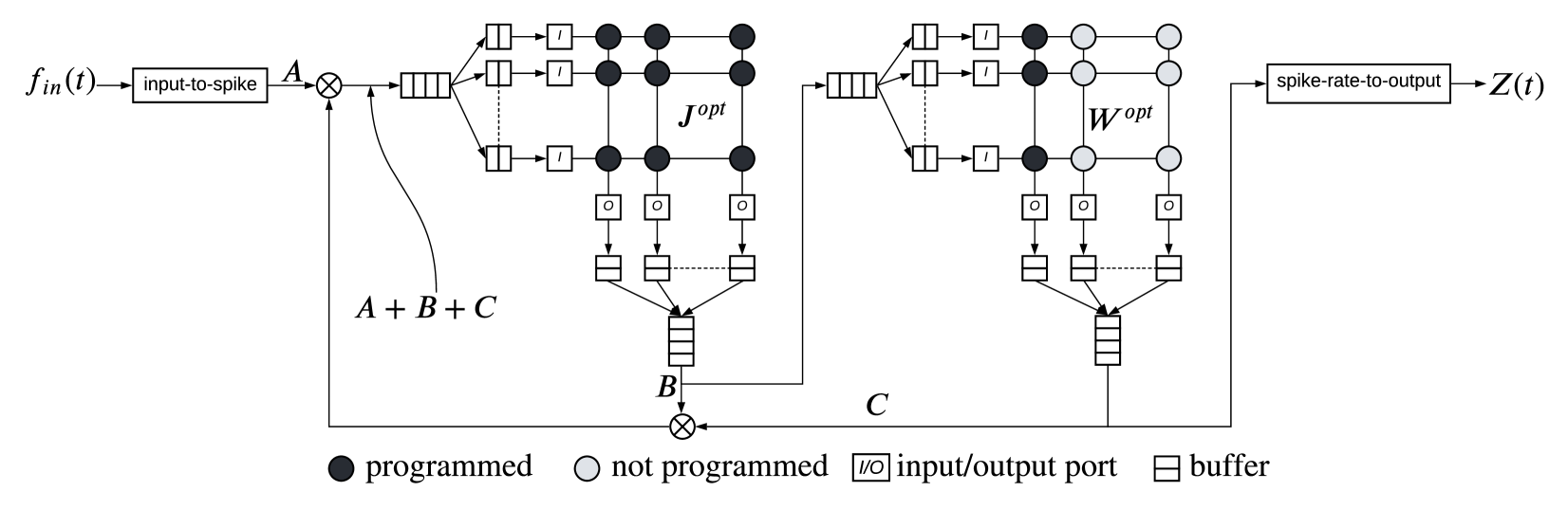
Figure 4: Implementation of the proposed trained RSNN on crossbar-based neuromorphic hardware.

The LIF neuron model provides a formalism of neuron firing rate in terms of a neuron’s membrane time constant, the threshold voltage and the refractory period. Therefore, for full-FORCE training of LIF neurons, $Y(t)$ in Equations 6, 7, & 10-15 are all interpreted in terms of spike rate.

The LIF neuron model is described by the dynamics of a neuron’s membrane voltage $V(t)$ due to input current $I(t)$ as

$$\footnotesize C\frac{dV(t)}{dt}=I_{\text{Bias}}+I(t),$$ (16)

where $C$ is the membrane capacitance and $I_{\text{Bias}}$ is the bias current. If $V(t)\geq V_{th}$, the neuron fires a spike, which is represented as [33]

$$\footnotesize I_{\text{spike}}(t)=C\left[\frac{dV(t)}{dt}\right]_{V(t)=V_{th}}^{-1}(V_{\text{rest}}-V_{th})\cdot\delta\Big{(}V(t)-V_{th}\Big{)}$$ (17)

Following a spike firing, the membrane voltage leaks over time. The voltage dynamics is

$$\footnotesize V(t)=I(t)\cdot R\cdot\left[1-e^{\frac{-t}{\tau}}\right],$$ (18)

where $R$ is the membrane resistance and $\tau=\frac{1}{R\cdot C}$ is the membrane time constant.

The inter-spike interval, defined as the time it takes to reach the membrane potential $V_{th}$ is calculated as

$$\footnotesize t_{\text{isi}}=-\tau\ln{\left(1-\frac{V_{th}}{I(t)\cdot R}\right)}=-\tau\ln{\left(1-\frac{I_{\text{rh}}}{I(t)}\right)},$$ (19)

where $I_{\text{rh}}$ is the rheobasic current, defined as the smallest current that drives the membrane voltage to $V_{th}$, i.e.,

$$\footnotesize I_{\text{rh}}=\frac{V_{th}}{R}$$ (20)

The spike firing rate is

$$\footnotesize R(t)=G\Big{(}I(t)\Big{)}=\frac{1}{\tau_{\text{ref}}+t_{\text{isi}}}=\frac{1}{\tau_{\text{ref}}-\tau\ln{\left(1-\frac{I_{\text{rh}}}{I(t)}\right)}},$$ (21)

where $\tau_{\text{ref}}$ is the refractory period.

Considering current synapses, the input to a neuron is computed as

$$\footnotesize I(t)=\sum_{i}w_{i}\sum_{k}\delta(t-t^{i}_{k}),$$ (22)

where $w_{i}$ is the synaptic weight connecting the $i^{\text{th}}$ input neuron, and $\sum_{k}\delta\big{(}t-t^{i}_{k}\big{)}$ are the spike trains of this input neuron with $t^{i}_{k}$ being the time of its $k^{\text{th}}$ spike. Here, $\delta(.)$ is the Dirac Delta function used to represent a spike. Considering $\bigintsss\delta(t)=1$ and a time interval $\Delta t$ for evaluating the spike rate,

$$\footnotesize I(t)=\sum_{i}w_{i}\cdot R_{i}\cdot\Delta t,$$ (23)

where $R_{i}$ is the spike rate of the $i^{\text{th}}$ input neuron.

To explain the full-FORCE training procedure for LIF neurons, consider the input $f_{in}(t)$ at time $t$ be converted to spike trains using an analog-to-spike converter [21]. It samples the instantaneous value of the input at time $t$ and uses it to create spike trains whose inter-spike interval follows a Poisson process with a mean firing rate equal to the sampled value of the input. These Poisson spikes excite spiking neurons in the two reservoirs of Figure 2b.

Output of the task-performing network is

$$\footnotesize Z(t)=G\Big{(}W^{T}\cdot R(t)\cdot\Delta t\Big{)},$$ (24)

where $R(t)$ is the spike rate of neurons in the task-performing network, $R(t)\cdot\Delta t$ computes the total number of spikes, $W^{T}\cdot R(t)\cdot\Delta t$ computes the current (see Eq. 23), and $G(\cdot)$ computes the resultant spike rate using Equation 21.

Dynamics of the task-performing network is

$$\footnotesize C\frac{dV(t)}{dt}=I(t)=\Big{(}J\cdot R(t)+U_{i}^{T}\cdot F_{in}(t)\Big{)}\cdot\Delta t,$$ (25)

where $F_{in}(t)=f_{in}(t)\cdot\mathbf{I}$ with $\mathbf{I}$ being the identity matrix. Observe the similarity of Equations 25 and 10.

Next, the membrane voltage is evaluated and output spike trains are generated using Equation 17. Finally, the output spike rate $R(t)$ is computed using Equation 21.

Using a similar formulation, dynamics of the target-generating network is computed as

$$\footnotesize C\frac{dV^{D}(t)}{dt}=I^{D}(t)=\Big{(}J^{D}\cdot R^{D}(t)+U_{i}^{T}\cdot F_{in}(t)+U_{o}\cdot Z(t)\Big{)}\cdot\Delta t,$$ (26)

We apply full-FORCE weight updates as follows.

1. $W$ updates are performed using Equations 6 & 7.

2. $J$ updates are performed using Equations 13 & 15.

In Section III-B, we show how the LIF neurons can be implemented in hardware and mapped to a platform using NeuroXplorer [34] or other similar frameworks.

III-B Hardware Implementation

Consider the proposed full-FORCE training procedure is implemented in software using PyCARL [35], CARLsim [36], or Nengo [37]. Subsequently, the trained weights ($J^{opt}$ and $W^{opt}$) are mapped to the hardware. Figure 4 shows one possible implementation of a trained RSNN on a crossbar-based neuromorphic hardware such as the DYNAPs [2]. In the future, we will demonstrate implementation on other architectures such as Loihi [4], and $\mu$Brain [3].

A crossbar is a two dimensional organization of wordlines and bitlines. A synaptic cell is placed at the intersection of each wordline and bitline [38]. A synaptic cell can be designed using non-volatile memory (NVM) [39].

Buffers are implemented at the input and output of a crossbar to store spikes, which are encoded in Address Event Representation (AER) format. Each input port of a crossbar (marked ’I’ in the figure) generates a voltage pulse for each AER packet stored in its input buffer. This voltage is multiplied with the conductance of a synaptic cell to generate a current. On an output port, which represents a post-synaptic neuron, current from different input ports are integrated (Kirchoff’s current law). This is the input current $I(t)$ which modulates a neuron’s membrane voltage $V(t)$ using the LIF dynamics described in Equations 16-21. Each output spike is converted to AER format and stored in the output buffer for transmission over the shared communication channel.

The RSNN architecture can be implemented on two $N\times N$ crossbars as shown in the figure. Here $N$ is the number of neurons in the reservoir of Figure 2. These crossbars implement matrices $J^{opt}$ and $W^{opt}$, respectively.

The reservoir network (crossbar 1) receives input spikes from three sources – the input signal $f_{in}(t)$ converted to spike (marked $A$), the recurrent connection from other neurons in the reservoir (marked $B$), and the output from the readout (crossbar 2) fed back to the reservoir (marked $C$). Observe, the recurrent connections of the reservoir neurons are implemented as a feedforward architecture in crossbar 1 with the output of the crossbar fed back to the input. The spike rate computed at the output of crossbar 2 is interpreted as the output $Z(t)$ of the RSNN architecture.

The design of Figure 4 can be implemented on a custom hardware using the Neural Engineering Framework (NEF) [40], NeuroXplorer [34], and SpiNeMap [41]. Alternatively, the SODASNN framework can be used to synthesize the above design on a Field Programmable Gate Array (FPGA) device [42]. We limit our discussion to implementing an RSNN on a crossbar-based neuromorphic hardware. To this end, the design flow of [43, 44, 45] can be used. A comprehensive overview of other frameworks and mapping flows can be found in [46]. We use NeuroXplorer [34]. For crossbar-based designs, spike communication between the computational units (input unit, crossbars, and output unit) takes place via a shared interconnect such as Network-on-Chip (NoC) or Segmented Bus [47, 48, 49].

A critical limitation of a crossbar-based neuromorphic hardware is the constraint on the size of a crossbar. Crossbars are designed as an $N\times N$ hardware with $N$ inputs and $N$ outputs. The typical value of $N$ ranges between 128 and 256 [50, 51, 52]. Therefore, if a reservoir contains more neurons than what can be accommodated on a crossbar, the reservoir network needs to be decomposed into smaller sub-networks using for instance, the spatial decomposition technique of [53]. Subsequently, each decomposed network can be mapped to an individual crossbar of the hardware. To demonstrate our full-FORCE learning, here we use crossbar sizes that can map each reservoir in its entirety, i.e., no spatial decomposition is necessary. Area-accuracy tradeoffs associated with spatial decomposition for full-FORCE will be addressed in the future.

Although using LIF neurons with rate coding simplifies the implementation, such coding generally leads to a higher number of spikes [54] (see our results in Section V). Following are the two critical neuromorphic design issues associated with having more spikes. First, higher spike count leads to an increase in the network congestion (i.e., delay) and energy consumption on the shared interconnect [55, 56, 57]. Second, it increases the buffer requirement on input and output ports of each crossbar [43], which increases the design cost (area and power) of an RSNN implementation.

III-C full-FORCE Training with TTFS Coding

In this coding scheme, the first spike generated from a neuron is prioritized over subsequent spikes from the same neuron [54]. Implementation-wise, a neuron follows the LIF dynamics described in Section III-A. However, there are two modifications necessary to implement TTFS coding.

First, instead of keeping the threshold voltage constant as in rate coding, here the threshold voltage $V_{th}$ is time dependant and is described using an exponential function

$$\footnotesize V_{th}(t)=\theta_{0}\cdot e^{\frac{-t}{\tau}},$$ (27)

where $\theta_{0}$ is a constant.

Second, inhibition behavior is implemented such that once a neuron fires a spike, it is inhibited from generating spikes until the next input arrives [58]. To do so, we introduce spike weights $w_{s}(t)$ in Equation 22. Specifically, the modified spike trains from a post-synaptic neuron are represented as

$$\footnotesize\text{spike trains}=w_{s}(t)\sum_{k}\delta(t-t^{i}_{k}),$$ (28)

where

$$\footnotesize w_{s}(t)=e^{\frac{-t}{\tau_{s}}}.$$ (29)

Here, $\tau_{s}$ is the time constant for spike inhibition.

IV Evaluation Framework

IV-A Algorithm Implementation

We implemented full-FORCE training in Python and simulated it on a Lambda workstation, which has AMD Threadripper 3960X with 24 cores, 128 MB cache, 128 GB RAM, and two RTX3090 GPUs. The code is available online at https://github.com/drexel-DISCO/SNN-full-FORCE.

IV-B Evaluated Dynamical Systems

We evaluate 8 dynamical system which are as follows.

1. Sine: The sine function $y(t)=\texttt{sine}(\omega\cdot t)$ is commonly used to represent a periodic dynamical system.

2. Sum of Sines: This is the sum of two sine functions with 4Hz and 6Hz frequencies, respectively.

3. Product of Sines: This is the product of two sine functions with 4Hz and 6Hz frequencies, respectively.

4. Accordian: This is an oscillatory signal that repeats periodically every 2s. This is represented using $y(t)=\texttt{sine}(\omega\cdot t)$. However, the frequency increases linearly from $2\pi$ to $6\pi$ Hz for the first half of the oscillation period, and then decreases linearly from $6\pi$ to $2\pi$ Hz during the second half of the oscillation period.

5. Ode-to-Joy: This is the 5-component signal representing the Ode-to-Joy notes by Beethoven, where each component corresponds to musical notes C-G. A note is represented with an upward pulse in the signal. Quarter notes are the positive parts of a 2 Hz sine wave and half notes are the positive parts of a 1 Hz sine wave.

6. Triangle: This is a triangular-shaped waveform that is represented by $y(t)=\texttt{(2a/$\pi$){arcsin}({sine}(2$\pi$}/p)x)$.

7. Van der Pol Harmonic: This is a non-conservatory oscillator discovered by Van der Pol and is represented as $\ddot{x}=\mu(1-x^{2})\dot{x}-x$ with $\mu=0.3$.

8. Van der Pol Relaxed: This is a relaxed form of the Van der Pol oscillator with $\mu$ set to 0.5.

Figures 5 (top and bottom) shows the target $f_{out}(t)$ and response $Z(t)$ for the dynamical systems representing the Accordian and Triangle functions, respectively.

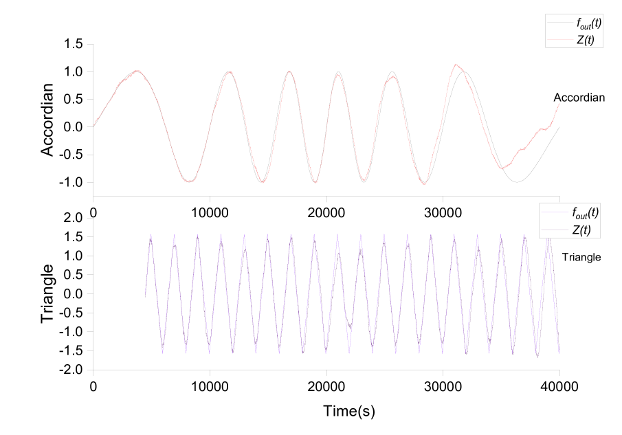
Figure 5: Target $f_{out}$(t) and response $Z(t)$ for the Accordian function (top) and Triangule function (bottom) using full-FORCE with rate coding.

IV-C Evaluated Training Procedure

We evaluate the following three training procedures.

1. FORCE-LIF-Rate: This is the FORCE training with LIF neurons and rate coding [29]. Here, only the readout weights $W$ are trained.

2. full-FORCE-LIF-Rate: This is our full-FORCE training with LIF neurons and rate coding. Here, both the reservoir wights $J$ and output weights $W$ are trained.

3. full-FORCE-LIF-TTFS: This is our full-FORCE training with LIF neurons and TTFS coding.

IV-D Evaluated Metrics

We evaluate the following three metrics

1. Mean Square Error (MSE): This is defined as the sum of the squared difference of the target and prediction, averaged over a fixed number of time steps. This is computed as follows.

   $$\footnotesize\texttt{MSE}=\frac{1}{n}\sum_{i=1}^{n}\Big{(}Z(t)-f_{out}(t)\Big{)}^{2}$$ (30)

2. Time to Converge (TTC): This is the number of epochs it takes to train an RSNN to mimick a target dynamical system.

3. Average Spike Rate (SR): This is the total number of spikes generated by all neurons in an RSNN averaged over a time interval.

V Results and Discussion

V-A Mean Square Error (MSE)

Table II reports the MSE for the evaluated training procedures for all eight dynamical systems (lower MSE is better). The experimental setup is as follows. The number of neurons in the RSNN reservoir is set to 1000 for FORCE-LIF-Rate and full-FORCE-LIF-Rate. For full-FORCE-LIF-TTFS, this is set to 200. These numbers are decided based on the following considerations. The number of neurons for the full-FORCE training procedure (both rate coding and TTFS coding) is configured to keep the MSE less than 0.35 for all evaluated dynamical systems. This MSE constraint of 0.35 is user configurable. To achieve this constraint, the full-FORCE training procedure with rate coding requires 1000 neurons while TTFS coding requires only 200 neurons. We also set the number of neurons in the reservoir for the FORCE training with rate coding to 1000 (i.e., the same as full-FORCE with rate coding). For all three training procedures, the number of training epochs is set to 50. We make the following three key observations.

TABLE II: MSE of Proposed full-FORCE (rate and TTFS) against state-of-the-art FORCE.

	FORCE-LIF-Rate (SOTA)	full-FORCE-LIF-Rate (Proposed)	full-FORCE-LIF-TTFS (Proposed)
Sine	0.041	0.009	0.32
Sum of Sines	0.470	0.250	0.240
Product of Sines	0.393	0.330	0.330
Accordian	0.909	0.03	0.2
Ode-to-Joy	0.701	0.002	0.02
Triangle	0.044	0.018	0.244
Van der Pol H.	0.048	0.048	0.15
Van der Pol R.	0.009	0.008	0.08

First, the MSE using FORCE is higher than the MSE constraint of 0.35 for four of the eight dynamical systems (Sum of Sines, Product of Sines, Accordian, and Ode-to-Joy). This means that for these systems a bigger reservoir (more than 1000 neurons) and possibly more training epochs are needed. For all eight dynamical systems, full-FORCE with rate coding satisfies the MSE constraint using 1000 neurons.

Second, the MSE using full-FORCE is lower than FORCE by an average of 51% (between 0.1% and 99.7%). This is due to its supervised training of both the reservoir weights $J$ and readout weights $W$. The FORCE training, on the other hand, trains only the readout weights. Furthermore, neurons are fully-connected in the reservoir to model systems that cannot be represented using closed-form differential equations. Therefore, the full-FORCE training procedure can train the reservoir more efficiently than FORCE.

Third, the MSE of full-FORCE with TTFS coding is higher than rate coding by a factor of 10x (on average). Although the MSE is higher (meaning the performance is lower), full-FORCE with TTFS coding satisfies the MSE constraint of 0.35. The key advantage of the TTFS coding is the reduced number of neurons required to achieve the MSE constraint. With only 200 neurons, i.e., 5x lower number of neurons than rate coding, full-FORCE is able to meet the MSE constraint for all dynamical systems. This is an important consideration for the hardware implementation because fewer the number of neurons, smaller is the hardware area and power consumption.

To give more insights to these results, Figures 6 shows the comparative performance of the full-FORCE training with rate coding and TTFS coding for the dynamical system represented using the Sum of Sines function.

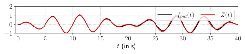
(a) $f_{out}(t)$ abd $Z(t)$ for full-FORCE training with rate coding.

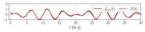
(b) $f_{out}(t)$ abd $Z(t)$ for full-FORCE training with TTFS coding.

Figure 6: Comparative performance of rate coding and TTFS coding for the sum-of-sine dynamical system.

Key takeaway points from these results are the following.

1. With the same number of neurons in an RSNN reservoir (hardware constraint), the full-FORCE training with rate coding leads to a lower MSE than FORCE.

2. To achieve a given MSE constraint, the full-FORCE with TTFS coding requires fewer neurons than both the FORCE and full-FORCE with rate coding.

V-B Time to Converge

Table  III reports the number of epochs it takes for each training procedure to reach an MSE of 0.25 in each epoch with 200 neurons. We make three key observations. First, between FORCE and full-FORCE with rate coding, FORCE requires a smaller number of epochs to converge. Second, full-FORCE with TTFS coding requires fewer epochs (on average) to converge compared to full-FORCE with rate coding. Third, full-FORCE with TTFS coding requires more epochs to converge for Van der Pol Harmonics and Van der Pol Relaxed due to their deterministic chaotic behavior.

TABLE III: Time to Converge of Proposed full-FORCE RSNN (rate and TTFS) against FORCE.

	FORCE-LIF-Rate (SOTA)	full-FORCE-LIF-Rate (Proposed)	full-FORCE-LIF-TTFS (Proposed)
Sine	2.29	2.85	0.18
Sum of Sines	2.39	1.8	1.43
Product of Sines	2.38	3.19	1.19
Accordian	1.55	1.95	1.39
Ode-to-Joy	3.06	4.48	3.05
Triangle	2.33	2.86	1.49
Van der Pol H.	3.52	4.9	4.15
Van der Pol R.	3.67	5.8	3.99

V-C Average Spike Rate

Figure 7 plots the spike rate of full-FORCE with TTFS coding normalized to rate coding for the eight evaluated dynamical systems. Results are reported for 200 and 1000 neurons in the RSNN reservoir. We make the following two key observations.

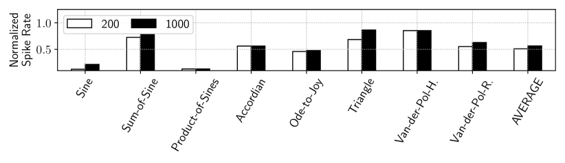
Figure 7: Spike rate for the evaluated dynamical systems with 200 and 1000 neurons in the RSNN reservoir.

First, TTFS coding results in fewer spikes than rate coding for all two sizes of the reservoir and across all eight dynamical systems. This is because of the nature of TTFS coding, where instead of communicating all spikes as in rate coding, information is represented by the relative time of arrival of the spikes with respect to the first spike. On average, TTFS generates 50% fewer spikes than rate coding.

Second, with more neurons in the reservoir, the number of spikes increases only marginally (average 15%) for the TTFS coding. The spike count for rate coding increases proportionately with the number of neurons.

V-D Noise Performance

We test the noise robustness using an RSNN reservoir with 600 neurons. We use 50 training epochs and add 10% Gaussian noise to the input signal. Table  IV reports the corresponding MSE. We observe that full-FORCE (both rate and TTFS coding) has lower MSE than FORCE demonstrating its noise robustness. However, due to using a single spike to encode information, full-FORCE with TTFS coding has a higher MSE than rate coding.

TABLE IV: MSE of evaluated training procedures with Gaussian Noise of Proposed full-FORCE RSNN (rate based and TTFS) against FORCE SNN (SOTA).

	FORCE-LIF-Rate (SOTA)	full-FORCE-LIF-Rate (Proposed)	full-FORCE-LIF-TTFS (Proposed)
Sine	0.23	0.048	0.2
Sum of Sines	0.85	0.02	0.23
Product of Sines	0.33	0.24	0.35
Accordian	1.75	1.72	1.739
Ode-to-Joy	0.75	0.05	0.135
Triangle	0.08	0.074	0.25
Van der Pol H.	0.223	0.17	0.199
Van der Pol R.	0.197	0.102	0.15

V-E Interval Matching Task

We train an RSNN for an interval matching task, where the objective is to learn the time interval between two pulses. The RSNN is excited with two input pulses, each with an amplitude of 1.0 and a time duration of 50ms. The RSNN is expected to generate an output response at a delay equal to the interval between the first and second pulse. Figure 9 plots the MSE of proposed full-FORCE training with rate and TTFS coding compared to the FORCE training. Results are reported for different interval matching tasks with intervals ranging from 0.1 to 2.1 in increment of 0.25. We observe that the MSE of full-FORCE training (both rate and TTFS coding) is lower than the FORCE.

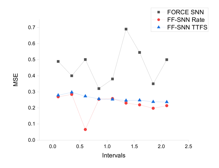
Figure 8: MSE for interval matching task with the time interval between two pulses ranging from 0.1 to 2.1 in increment of 0.25.

VI Conclusion

We propose a supervised training procedure, called full-FORCE for feedback-driven reservoir computing architecture with input, reservoir, and readout layers, each of which is designed using Leaky Integrate and Fire (LIF) neurons. The objective is to model dynamical systems. The full-FORCE training procedure introduces a second recurrently-connected reservoir network only during the training to provide hints for the target dynamics. It then uses the recursive least square-based First-Order and Reduced Control Error (FORCE) algorithm to fit the activity of the reservoir and the readout to their corresponding target. We demonstrate the improved performance and noise robustness of the full-FORCE training to model 8 dynamical systems using LIF neurons with rate coding. For energy-efficient hardware implementation, an alternative time-to-first-spike (TTFS) coding scheme is also presented for the full-FORCE training. Compared to rate coding, full-FORCE with TTFS coding requires lower spike count and facilitates faster convergence to the target dynamics.

References

- [1] W. Maass, “Networks of spiking neurons: The third generation of neural network models,” Neural Networks, 1997.
- [2] S. Moradi, N. Qiao, F. Stefanini, and G. Indiveri, “A scalable multicore architecture with heterogeneous memory structures for dynamic neuromorphic asynchronous processors (DYNAPs),” TBCAS, 2017.
- [3] M. L. Varshika, A. Balaji, F. Corradi, A. Das, J. Stuijt, and F. Catthoor, “Design of many-core big little Brains for energy-efficient embedded neuromorphic computing,” in DATE, 2022.
- [4] M. Davies, N. Srinivasa, T. H. Lin et al., “Loihi: A neuromorphic manycore processor with on-chip learning,” IEEE Micro, 2018.
- [5] A. R. Voelker, “Dynamical systems in spiking neuromorphic hardware,” 2019.
- [6] M. Han, Z. Shi, and W. Wang, “Modeling dynamic system by recurrent neural network with state variables,” in ISNN, 2004.
- [7] M. Lukoševičius and H. Jaeger, “Reservoir computing approaches to recurrent neural network training,” Computer Science Review, 2009.
- [8] D. J. Gauthier, E. Bollt, A. Griffith, and W. A. Barbosa, “Next generation reservoir computing,” Nature Communications, 2021.
- [9] G. Tanaka, T. Yamane, J. B. Héroux, R. Nakane, N. Kanazawa, S. Takeda, H. Numata, D. Nakano, and A. Hirose, “Recent advances in physical reservoir computing: A review,” Neural Networks, 2019.
- [10] S. Li, B. Liu, and Y. Li, “Selective positive–negative feedback produces the winner-take-all competition in recurrent neural networks,” TNNLS, 2012.
- [11] G. Bellec, F. Scherr, A. Subramoney, E. Hajek, D. Salaj, R. Legenstein, and W. Maass, “A solution to the learning dilemma for recurrent networks of spiking neurons,” Nature Communications, 2020.
- [12] Y. Bengio, P. Simard, and P. Frasconi, “Learning long-term dependencies with gradient descent is difficult,” TNNLS, 1994.
- [13] R. Pascanu, T. Mikolov, and Y. Bengio, “On the difficulty of training recurrent neural networks,” in ICML, 2013.
- [14] J. Chung, C. Gulcehre, K. Cho, and Y. Bengio, “Gated feedback recurrent neural networks,” in ICML, 2015.
- [15] Y. Bengio, N. Boulanger-Lewandowski, and R. Pascanu, “Advances in optimizing recurrent networks,” in ICASSP. IEEE, 2013.
- [16] K. Rajan, L. Abbott, and H. Sompolinsky, “Stimulus-dependent suppression of chaos in recurrent neural networks,” Physical Review E, 2010.
- [17] D. Sussillo and L. F. Abbott, “Generating coherent patterns of activity from chaotic neural networks,” Neuron, 2009.
- [18] H. Soula, G. Beslon, and O. Mazet, “Spontaneous dynamics of asymmetric random recurrent spiking neural networks,” Neural Computation, 2006.
- [19] R. Engelken, F. Wolf, and L. F. Abbott, “Lyapunov spectra of chaotic recurrent neural networks,” arXiv, 2020.
- [20] W. Maass, T. Natschläger, and H. Markram, “Real-time computing without stable states: A new framework for neural computation based on perturbations,” Neural Computation, 2002.
- [21] A. Das, P. Pradhapan, W. Groenendaal, P. Adiraju, R. Rajan, F. Catthoor, S. Schaafsma, J. Krichmar, N. Dutt, and C. Van Hoof, “Unsupervised heart-rate estimation in wearables with Liquid states and a probabilistic readout,” Neural Networks, 2018.
- [22] B. J. Grzyb, E. Chinellato, G. M. Wojcik, and W. A. Kaminski, “Which model to use for the liquid state machine?” in IJCNN, 2009.
- [23] P. J. Werbos, “Backpropagation through time: what it does and how to do it,” Proceedings of the IEEE, 1990.
- [24] W. Zhang and P. Li, “Spike-train level backpropagation for training deep recurrent spiking neural networks,” NeurIPS, 2019.
- [25] W. Zhang and P. Li, “Temporal spike sequence learning via backpropagation for deep spiking neural networks,” NeurIPS, pp. 12 022–12 033, 2020.
- [26] W. Zhang and P. Li, “Spiking neural networks with laterally-inhibited self-recurrent units,” in IJCNN, 2021.
- [27] N. Caporale and Y. Dan, “Spike timing–dependent plasticity: a hebbian learning rule,” Annu. Rev. Neurosci., 2008.
- [28] S. Hochreiter, “The vanishing gradient problem during learning recurrent neural nets and problem solutions,” International Journal of Uncertainty, Fuzziness and Knowledge-Based Systems, 1998.
- [29] W. Nicola and C. Clopath, “Supervised learning in spiking neural networks with FORCE training,” Nature Communications, 2017.
- [30] H.-G. Zimmermann, R. Neuneier, and R. Grothmann, “Modeling dynamical systems by error correction neural networks,” in Modelling and Forecasting Financial Data. Springer, 2002, pp. 237–263.
- [31] S. H. Lim, N. B. Erichson, L. Hodgkinson, and M. W. Mahoney, “Noisy recurrent neural networks,” NeurIPS, 2021.
- [32] B. DePasquale, C. J. Cueva, K. Rajan, G. S. Escola, and L. F. Abbott, “full-FORCE: A target-based method for training recurrent networks,” PLOS ONE, 2018.
- [33] H. Meffin, A. N. Burkitt, and D. B. Grayden, “An analytical model for the ‘large, fluctuating synaptic conductance state’typical of neocortical neurons in vivo,” Journal of Computational Neuroscience, 2004.
- [34] A. Balaji, S. Song, T. Titirsha, A. Das, J. Krichmar, N. Dutt, J. Shackleford, N. Kandasamy, and F. Catthoor, “NeuroXplorer 1.0: An extensible framework for architectural exploration with spiking neural networks,” in ICONS, 2021.
- [35] A. Balaji, P. Adiraju, H. J. Kashyap, A. Das, J. L. Krichmar, N. D. Dutt, and F. Catthoor, “PyCARL: A PyNN interface for hardware-software co-simulation of spiking neural network,” in IJCNN, 2020.
- [36] T. Chou, H. Kashyap, J. Xing, S. Listopad, E. Rounds, M. Beyeler, N. Dutt, and J. Krichmar, “CARLsim 4: An open source library for large scale, biologically detailed spiking neural network simulation using heterogeneous clusters,” in IJCNN, 2018.
- [37] T. Bekolay, J. Bergstra, E. Hunsberger, T. DeWolf, T. C. Stewart, D. Rasmussen, X. Choo, A. Voelker, and C. Eliasmith, “Nengo: a python tool for building large-scale functional brain models,” Frontiers in Neuroinformatics, 2014.
- [38] M. Hu, H. Li, Y. Chen, Q. Wu, G. S. Rose, and R. W. Linderman, “Memristor crossbar-based neuromorphic computing system: A case study,” TNNLS, 2014.
- [39] A. Mallik, D. Garbin, A. Fantini, D. Rodopoulos, R. Degraeve, J. Stuijt, A. Das, S. Schaafsma, P. Debacker, G. Donadio et al., “Design-technology co-optimization for OxRRAM-based synaptic processing unit,” in VLSIT, 2017.
- [40] C. Eliasmith and C. H. Anderson, Neural engineering: Computation, representation, and dynamics in neurobiological systems. MIT press, 2003.
- [41] A. Balaji, A. Das, Y. Wu, K. Huynh, F. G. Dell’anna, G. Indiveri, J. L. Krichmar, N. D. Dutt, S. Schaafsma, and F. Catthoor, “Mapping spiking neural networks to neuromorphic hardware,” TVLSI, 2020.
- [42] S. Curzel, N. B. Agostini, S. Song, I. Dagli, A. Limaye, C. Tan, M. Minutoli, V. G. Castellana, V. Amatya, J. Manzano et al., “Automated generation of integrated digital and spiking neuromorphic machine learning accelerators,” in ICCAD, 2021.
- [43] S. Song, L. V. Mirtinti, A. Das, and N. Kandasamy, “A design flow for mapping spiking neural networks to many-core neuromorphic hardware,” in ICCAD, 2021.
- [44] S. Song, H. Chong, A. Balaji, A. Das, J. Shackleford, and N. Kandasamy, “DFSynthesizer: Dataflow-based synthesis of spiking neural networks to neuromorphic hardware,” TECS, 2021.
- [45] S. Song, A. Balaji, A. Das, N. Kandasamy, and J. Shackleford, “Compiling spiking neural networks to neuromorphic hardware,” in LCTES, 2020.
- [46] P. K. Huynh, M. L. Varshika, A. Paul, M. Isik, A. Balaji, and A. Das, “Implementing spiking neural networks on neuromorphic architectures: A review,” arXiv preprint arXiv:2202.08897, 2022.
- [47] X. Liu, W. Wen, X. Qian, H. Li, and Y. Chen, “Neu-NoC: A high-efficient interconnection network for accelerated neuromorphic systems,” in ASP-DAC, 2018.
- [48] A. Balaji, Y. Wu, A. Das, F. Catthoor, and S. Schaafsma, “Exploration of segmented bus as scalable global interconnect for neuromorphic computing,” in GLSVLSI, 2019.
- [49] F. Catthoor, S. Mitra, A. Das, and S. Schaafsma, “Very large-scale neuromorphic systems for biological signal processing,” in CMOS Circuits for Biological Sensing and Processing, 2018.
- [50] A. Paul and A. Das, “Design technology co-optimization for neuromorphic computing,” in IGSC Workshops, 2021.
- [51] S. Song, A. Balaji, A. Das, and N. Kandasamy, “Design-technology co-optimization for nvm-based neuromorphic processing elements,” TECS, 2022.
- [52] T. Titirsha, S. Song, A. Balaji, and A. Das, “On the role of system software in energy management of neuromorphic computing,” in CF, 2021.
- [53] A. Balaji, S. Song, A. Das, J. Krichmar, N. Dutt, J. Shackleford, N. Kandasamy, and F. Catthoor, “Enabling resource-aware mapping of spiking neural networks via spatial decomposition,” ESL, 2020.
- [54] S. Park, S. Kim, B. Na, and S. Yoon, “T2FSNN: Deep spiking neural networks with time-to-first-spike coding,” in DAC, 2020.
- [55] F. Barchi, G. Urgese, E. Macii, and A. Acquaviva, “Mapping spiking neural networks on multi-core neuromorphic platforms: Problem formulation and performance analysis,” in VLSI-SoC, 2018.
- [56] G. Urgese, F. Barchi, E. Macii, and A. Acquaviva, “Optimizing network traffic for spiking neural network simulations on densely interconnected many-core neuromorphic platforms,” TETC, 2016.
- [57] A. Das, Y. Wu, K. Huynh, F. Dell’Anna, F. Catthoor, and S. Schaafsma, “Mapping of local and global synapses on spiking neuromorphic hardware,” in DATE, 2018.
- [58] J. Göltz, A. Baumbach, S. Billaudelle, O. Breitwieser, D. Dold, L. Kriener, A. F. Kungl, W. Senn, J. Schemmel, K. Meier et al., “Fast and deep neuromorphic learning with time-to-first-spike coding,” arXiv, 2019.