Efficient Approximation of Gromov-Wasserstein Distance Using Importance Sparsification

Abstract

As a valid metric of metric-measure spaces, Gromov-Wasserstein (GW) distance has shown the potential for matching problems of structured data like point clouds and graphs. However, its application in practice is limited due to the high computational complexity. To overcome this challenge, we propose a novel importance sparsification method, called Spar-GW, to approximate GW distance efficiently. In particular, instead of considering a dense coupling matrix, our method leverages a simple but effective sampling strategy to construct a sparse coupling matrix and update it with few computations. The proposed Spar-GW method is applicable to the GW distance with arbitrary ground cost, and it reduces the complexity from $O(n^{4})$ to $O(n^{2+\delta})$ for an arbitrary small $\delta>0$. Theoretically, the convergence and consistency of the proposed estimation for GW distance are established under mild regularity conditions. In addition, this method can be extended to approximate the variants of GW distance, including the entropic GW distance, the fused GW distance, and the unbalanced GW distance. Experiments show the superiority of our Spar-GW to state-of-the-art methods in both synthetic and real-world tasks.

Keywords: Element-wise sampling, Importance sampling, Sinkhorn-scaling algorithm, Unbalanced Gromov-Wasserstein distance

1 Introduction

Gromov-Wasserstein (GW) distance, as an extension of classical optimal transport distance, is originally proposed to measure the distance between different metric-measure spaces (Mémoli,, 2011; Sturm,, 2006). Recently, it attracts wide attention due to its potential for tackling challenging machine learning tasks, including but not limited to shape matching (Mémoli,, 2011; Ezuz et al.,, 2017; Titouan et al., 2019b, ), graph analysis (Chowdhury and Mémoli,, 2019; Xu et al., 2019b, ; Titouan et al., 2019a, ; Chowdhury and Needham,, 2021; Brogat-Motte et al.,, 2022; Vincent-Cuaz et al.,, 2022; Xu et al.,, 2023), point cloud alignment (Peyré et al.,, 2016; Alvarez-Melis and Jaakkola,, 2018; Alaux et al.,, 2019; Blumberg et al.,, 2020), and distribution comparison across different spaces (Yan et al.,, 2018; Bunne et al.,, 2019; Chapel et al.,, 2020; Gong et al.,, 2022).

Despite the wide application, calculating the GW distance is NP-hard, which corresponds to solving a non-convex non-smooth optimization problem. To bypass this obstacle, many efforts have been made to approximate the GW distance with low complexity. One major strategy is applying the conditional gradient algorithm (or its variants) to solve the GW distance iteratively in an alternating optimization framework (Peyré et al.,, 2016; Titouan et al., 2019a, ). By introducing an entropic regularizer (Solomon et al.,, 2016) or a proximal term based on the Bergman divergence (Xu et al., 2019b, ), the subproblem in each iteration will be strictly convex and can be solved via the Sinkhorn-scaling algorithm (Sinkhorn and Knopp,, 1967; Cuturi,, 2013). Another strategy is computing sliced Gromov-Wasserstein distance (Titouan et al., 2019b, ), which projects the samples to different 1D spaces and calculates the expectation of the GW distances defined among the projected 1D samples. More recently, to further reduce the computational complexity, more variants of the GW distance have been proposed, which achieve acceleration via imposing structural information (e.g., tree (Le et al.,, 2021), low-rank (Xu et al., 2019a, ; Sato et al.,, 2020; Chowdhury et al.,, 2021), and sparse structure (Xu et al., 2019a, )) on the ground cost $\mathcal{L}$, the coupling matrix $\mathbf{T}$, or both (Scetbon et al.,, 2022). However, most of these methods mainly focus on the GW distance using decomposable ground cost functions (Peyré et al.,, 2016). Moreover, some of them are only applicable for specific data types (e.g., point clouds in Euclidean space (Titouan et al., 2019b, ) and sparse graphs with clustering structures (Xu et al., 2019a, ; Blumberg et al.,, 2020)), and they are not able to approximate the original GW distance. See Table 1 for an overall comparison. Therefore, it is urgent to develop a new approximation of the GW distance that has better efficiency and applicability.

Table 1: Comparison for various GW distance approximation methods on their time complexity, assumptions imposed on their ground cost functions and coupling matrices, and required data types.

Method	Time $O(\cdot)$	Ground cost $\mathcal{L}$	Coupling $\mathbf{T}$	Data type
Entropic GW (Peyré et al.,, 2016)	$n^{3}$	Decomposable	-	-
Sliced GW (Titouan et al., 2019b, )	$n^{2}$	$\ell_{2}$ loss	-	Points
S-GWL (Xu et al., 2019a, )	$n^{2}\log(n)$	Decomposable	Sparse & low-rank	-
AE (Sato et al.,, 2020)	$n^{2}\log(n^{2})$	$p$-power ($p\in\mathbb{Z}_{+}$)	-	-
FlowAlign (Le et al.,, 2021)	$n^{2}$	$\ell_{2}$ loss	Tree-structure	Points
Linear-time GW (Scetbon et al.,, 2022)	$r_{2}(r_{1}+r_{2})n$	$\ell_{2}$ loss	Low-rank	Points
SaGroW (Kerdoncuff et al.,, 2021)	$n^{2}(s^{\prime}+\log(n))$	-	-	-
Spar-GW (Proposed)	$n^{2}+s^{2}$	-	-	-

• “-” means no constraints. For the column of data type, “-” means the data can be sample points and/or their relation matrices.

• For the column of time complexity, the time of calculating relation matrices of points is also included.

• $n$ represents the sample size. For Linear-time GW, $r_{1}$ and $r_{2}$ are the assumed ranks of relation matrices and coupling matrix, respectively; for SaGroW, $s^{\prime}$ denotes the number of sampled matrix; for Spar-GW, $s$ denotes the number of sampled elements.

Major contribution. In this paper, we propose a randomized sparsification method, called Spar-GW, to approximate the GW distance and its variants. In particular, during the iterative optimization of the GW distance, the proposed Spar-GW method leverages an importance sparsification mechanism to derive a sparse coupling matrix and the corresponding kernel matrix. Replacing dense multiplications with sparse ones leads to an efficient approximation of GW distance with $O(n^{2}+s^{2})$ time complexity, where $s$ is the number of selected elements from an $n\times n$ kernel matrix. The Spar-GW is compatible with various computational methods, including the proximal gradient algorithm for original GW distance and the Sinkhorn-scaling algorithm for entropic GW distance, and it is capable of arbitrary ground cost. In theory, we show the proposed estimator is asymptotically unbiased when $s=O(n^{1+\delta})$ for an arbitrary small $\delta>0$, under some regularity conditions. Table 1 highlights the advantage of our method. Moreover, this method can be extended to compute the variants of GW distance, e.g., a straightforward application to approximate the fused GW (FGW) distance and a non-trivial extension called Spar-UGW to approximate the unbalanced GW (UGW) distance. Experiments show the superiority of the proposed methods to state-of-the-art competitors in both synthetic and real-world tasks.

The remainder of this paper is organized as follows. We start in Section 2 by introducing computational optimal transport and GW distance. In Section 3, we develop the sampling probabilities and provide details of our main algorithm. The theoretical properties of the proposed estimator are presented in Section 4. Section 5 extends the proposed method to unbalanced problems. We examine the performance of the proposed algorithms through extensive synthetic and real-world datasets in Section 6. Technical proofs and more experimental results are provided in the Appendix.

2 Background

In the following, we adopt the common convention of using uppercase boldface letters for matrices, lowercase boldface letters for vectors, and regular font for scalars. We denote non-negative real numbers by $\mathbb{R}_{+}$ and the set of integers $\{1,\ldots,n\}$ by $[n]$. We use $\mathbf{1}_{n}$ and $\mathbf{0}_{n}$ to denote the all-ones and all-zeroes vectors in $\mathbb{R}^{n}$, respectively. For a matrix $\mathbf{A}=(A_{ij})$, its spectral norm (i.e., the largest singular value) and Frobenius norm are denoted as $\|\mathbf{A}\|_{2}$ and $\|\mathbf{A}\|_{F}$, respectively. The condition number of $\mathbf{A}$ is defined as $\|\mathbf{A}\|_{2}/\sigma_{\min}(\mathbf{A})$, where $\sigma_{\min}(\cdot)$ stands for the smallest singular value. We denote by $\exp(\mathbf{A})$ the matrix with entries $\exp(A_{ij})$. For two matrices $\mathbf{A}$ and $\mathbf{B}$ of the same dimension, we denote their Frobenius inner product by $\langle\mathbf{A},\mathbf{B}\rangle=\sum_{i,j}A_{ij}B_{ij}$.

2.1 Computational optimal transport

Consider two samples $X=\{\bm{x}_{i}\}_{i=1}^{m}$ and $Y=\{\bm{y}_{j}\}_{j=1}^{n}$ that are generated from the distributions $\bm{a}\in\Delta^{m-1}$ and $\bm{b}\in\Delta^{n-1}$, respectively, where $\Delta^{n-1}$ represents the $(n-1)$-Simplex. When $\bm{a}$ and $\bm{b}$ lie in the same space, optimal transport (OT) and its associated Wasserstein distance (Villani,, 2009) are used extensively to quantify the discrepancy between these two probability distributions. The modern Kantorovich formulation (Kantorovich,, 1942) of OT writes

$$\operatorname{W}(\bm{a},\bm{b}):=\min_{\mathbf{T}\in\Pi(\bm{a},\bm{b})}\langle\mathbf{M},\mathbf{T}\rangle,$$ (1)

where $\mathbf{M}\in\mathbb{R}^{m\times n}$ is a given distance matrix, $\Pi(\bm{a},\bm{b})=\{\mathbf{T}\in\mathbb{R}_{+}^{m\times n}:\mathbf{T}\mathbf{1}_{n}=\bm{a},\mathbf{T}^{\top}\mathbf{1}_{m}=\bm{b}\}$ is the set of admissible coupling matrices, i.e., all joint probability distributions with marginals $\bm{a},\bm{b}$, and the $(i,j)$-th entry of $\mathbf{T}$ represents the amount of probability mass shifted from $i$ to $j$. The solution to (1) is called the optimal transport plan. If $\mathbf{M}$ is a distance matrix of order $p$, $\operatorname{W}_{p}(\cdot,\cdot)=\operatorname{W}(\cdot,\cdot)^{1/p}$ is called the $p$-Wasserstein distance.

Despite the wide applications, the computational complexity of directly solving (1) using a linear program grows cubically as $m$ or $n$ increases (Brenier,, 1997; Benamou et al.,, 2002). To approximate the optimal transport plan efficiently, Cuturi, (2013) added an entropic regularization term on (1), which leads to a strongly convex and smooth problem

$$\min_{\mathbf{T}\in\Pi(\bm{a},\bm{b})}\langle\mathbf{M},\mathbf{T}\rangle+\varepsilon H(\mathbf{T}),$$ (2)

where $\varepsilon>0$ is a regularization parameter and $H(\mathbf{T})=\langle\mathbf{T},\log\mathbf{T}\rangle$ is the negative Shannon entropy of $\mathbf{T}$. By introducing a kernel matrix $\mathbf{K}:=\exp(-\mathbf{M}/\varepsilon)$, it is known that the solution to (2) is a projection onto $\Pi(\bm{a},\bm{b})$ of $\mathbf{K}$ (Peyré and Cuturi,, 2019). Therefore, the problem (2) can be solved by using iterative matrix scaling (Sinkhorn and Knopp,, 1967), called the Sinkhorn-scaling algorithm (Cuturi,, 2013); see Step 5 in Algorithm 1 for details. The Sinkhorn-scaling algorithm enables researchers to approximate the OT solution efficiently, and thus has been extensively studied in recent years (Genevay et al.,, 2019; Lin et al.,, 2019; Scetbon and Cuturi,, 2020; Liao et al., 2022a, ; Liao et al., 2022b, ). There also exist projection-based methods to approximate the Wasserstein distance (Bonneel et al.,, 2015; Meng et al.,, 2019; Deshpande et al.,, 2019; Li et al.,, 2022). We refer to Nadjahi, (2021) and Zhang et al., (2022) for recent reviews.

2.2 Computational GW distance

When $\bm{a}$ and $\bm{b}$ lie in different spaces, the distance matrix $\mathbf{M}$ is unavailable and thus optimal transport can not be used. As a replacement, the Gromov-Wasserstein distance is applicable to measuring the discrepancy between two samples located in different sample spaces by comparing their structural similarity. Similar to Wasserstein distance, the intuition of GW distance is still to minimize the transportation effort, but GW only relies on the structure in each space separately.

In particular, consider two relation matrices $\mathbf{C}^{X}=(C_{ii^{\prime}}^{X})\in\mathbb{R}^{m\times m}$ and $\mathbf{C}^{Y}=(C_{jj^{\prime}}^{Y})\in\mathbb{R}^{n\times n}$, each of which can be the distance/kernel matrix defined on a sample (Mémoli,, 2011; Peyré et al.,, 2016), or the adjacency matrix of a graph constructed by the sample (Xu et al., 2019b, ; Titouan et al., 2019a, ). Let $\mathcal{L}:\mathbb{R}\times\mathbb{R}\mapsto\mathbb{R}$ be the ground cost function, e.g., the $\ell_{1}$ loss (i.e., $\mathcal{L}(x_{1},x_{2})=|x_{1}-x_{2}|$), the $\ell_{2}$ loss (i.e., $\mathcal{L}(x_{1},x_{2})=(x_{1}-x_{2})^{2}$), and the Kullback-Leibler (KL) divergence (i.e., $\mathcal{L}(x_{1},x_{2})=x_{1}\log(x_{1}/x_{2})-x_{1}+x_{2}$). The GW distance is defined as the following non-convex non-smooth optimization problem:

$$\begin{aligned} \operatorname{GW}\left((\mathbf{C}^{X},\bm{a}),(\mathbf{C}^{Y},\bm{b})\right):=&\sideset{}{{}_{\mathbf{T}\in\Pi(\bm{a},\bm{b})}}{\min}\sideset{}{{}_{i,i^{\prime},j,j^{\prime}}}{\sum}\mathcal{L}\left(C_{ii^{\prime}}^{X},C_{jj^{\prime}}^{Y}\right)T_{ij}T_{i^{\prime}j^{\prime}}\\ =&\sideset{}{{}_{\mathbf{T}\in\Pi(\bm{a},\bm{b})}}{\min}\langle\mathcal{L}(\mathbf{C}^{X},\mathbf{C}^{Y})\otimes\mathbf{T},\mathbf{T}\rangle=\langle\mathcal{L}(\mathbf{C}^{X},\mathbf{C}^{Y})\otimes\mathbf{T}^{*},\mathbf{T}^{*}\rangle,\end{aligned}$$ (3)

where $\mathcal{L}(C_{ii^{\prime}}^{X},C_{jj^{\prime}}^{Y})$ measures similarity between pairs of points or graphs, $T_{ij}$ is the $(i,j)$-th entry of the coupling matrix $\mathbf{T}$, and then the term $\mathcal{L}\left(C_{ii^{\prime}}^{X},C_{jj^{\prime}}^{Y}\right)T_{ij}T_{i^{\prime}j^{\prime}}$ represents the transport cost between two pairs $(i,i^{\prime})$ and $(j,j^{\prime})$. As shown in (3), this optimization problem can be written in a matrix format (Peyré et al.,, 2016), where $\mathcal{L}(\mathbf{C}^{X},\mathbf{C}^{Y})$ is a tensor, and $\mathcal{L}(\mathbf{C}^{X},\mathbf{C}^{Y})\otimes\mathbf{T}:=[(\sum_{i^{\prime},j^{\prime}}\mathcal{L}(C^{X}_{ii^{\prime}},C^{Y}_{jj^{\prime}})T_{i^{\prime}j^{\prime}})_{i,j}]\in\mathbb{R}^{m\times n}$ is a tensor-matrix multiplication. As before, $\Pi(\bm{a},\bm{b})$ is the set of admissible coupling matrices, and the solution to problem (3), denoted as $\mathbf{T}^{\ast}$, is called the optimal transport plan.

In general, this optimization problem can be solved in an iterative framework: at the $r$-th iteration, the coupling matrix $\mathbf{T}$ is updated via solving the following subproblem:

$$\mathbf{T}^{(r+1)}:=\arg\sideset{}{{}_{\mathbf{T}\in\Pi(\bm{a},\bm{b})}}{\min}\langle\underbrace{\mathcal{L}(\mathbf{C}^{X},\mathbf{C}^{Y})\otimes\mathbf{T}^{(r)}}_{\mathcal{C}(\mathbf{T}^{(r)})},\mathbf{T}\rangle+\underbrace{\varepsilon\mathcal{R}(\mathbf{T})}_{\text{Optional Reg.}}.$$ (4)

Here, $\mathcal{C}(\mathbf{T}^{(r)})$ is a cost matrix determined by the previous coupling matrix $\mathbf{T}^{(r)}$, $\mathcal{R}(\mathbf{T})$ is an optional regularizer of $\mathbf{T}$, whose significance is controlled by the weight $\varepsilon\geq 0$. The subproblem is essentially the (regularized) optimal transport problem (1) or (2). Without $\mathcal{R}(\mathbf{T})$, the problem in (4) becomes a constrained linear programming given $\mathbf{T}^{(r)}$, and this is often solved via the conditioned gradient followed by line-search (Titouan et al., 2019a, ). To improve the efficiency of solving the problem, Xu et al., 2019b implements $\mathcal{R}(\mathbf{T})$ as a Bregman proximal term, i.e., the KL-divergence $\text{KL}(\mathbf{T}\|\mathbf{T}^{(r)})=\langle\mathbf{T},\log\mathbf{T}-\log\mathbf{T}^{(r)}\rangle$, which leads to a proximal gradient algorithm (PGA) and improves the smoothness of $\mathbf{T}$’s update. When the regularizer is implemented as the entropy of $\mathbf{T}$, i.e., $\mathcal{R}(\mathbf{T}):=H(\mathbf{T})$, the problem in (4) becomes an entropic optimal transport problem and solving it iteratively leads to the approximation of GW distance or entropic GW distance (Peyré et al.,, 2016). Note that, when using the Bregman proximal term or the entropic regularizer, the problem in (4) can be solved via the Sinkhorn-scaling algorithm (Sinkhorn and Knopp,, 1967; Cuturi,, 2013), and accordingly, Algorithm 1 shows the computational scheme of the GW distance, where $\odot$ and $\oslash$ represent element-wise multiplication and division, respectively. When $\mathcal{R}(\mathbf{T})=H(\mathbf{T})$, Algorithm 1 can also be used to compute the entropic GW distance by modifying the output to $\operatorname{GW}_{\varepsilon}=\langle\mathcal{C}(\mathbf{T}^{(R)}),\mathbf{T}^{(R)}\rangle+\varepsilon H(\mathbf{T}^{(R)})$.

Algorithm 1 Computation of GW distance

1:Input: Sample distributions $\bm{a},\bm{b}$, relation matrices $\mathbf{C}^{X},\mathbf{C}^{Y}$, ground cost function $\mathcal{L}$, regularization parameter $\varepsilon$, number of outer/inner iterations $R$, $H$

2:Initialize $\mathbf{T}^{(0)}=\bm{a}\bm{b}^{\top}$

3:For $r=0\textbf{ to }R-1$:

4:  Construct a kernel matrix: $O(m^{2}n^{2})$ a) Compute the cost matrix $\mathcal{C}(\mathbf{T}^{(r)})=\mathcal{L}(\mathbf{C}^{X},\mathbf{C}^{Y})\otimes\mathbf{T}^{(r)}$ b) $\mathbf{K}^{(r)}=\begin{cases}\exp(-\frac{\mathcal{C}(\mathbf{T}^{(r)})}{\varepsilon})\odot\mathbf{T}^{(r)}&\text{ if }\mathcal{R}(\mathbf{T})=\text{KL}(\mathbf{T}\|\mathbf{T}^{(r)})\\ \exp(-\frac{\mathcal{C}(\mathbf{T}^{(r)})}{\varepsilon})&\text{ if }\mathcal{R}(\mathbf{T})=H(\mathbf{T})\end{cases}$

5:  Sinkhorn-scaling: $\mathbf{T}^{(r+1)}=\textsc{Sinkhorn}(\bm{a},\bm{b},\mathbf{K}^{(r)},H)$ $O(Hmn)$ a) Initialize $\bm{u}^{(0)}=\mathbf{1}_{m},\bm{v}^{(0)}=\mathbf{1}_{n}$ b) For $h=0\textbf{ to }H-1$: $\bm{u}^{(h+1)}=\bm{a}\oslash(\mathbf{K}^{(r)}\bm{v}^{(h)})$,  $\bm{v}^{(h+1)}=\bm{b}\oslash(\mathbf{K}^{{}^{(r)}\top}\bm{u}^{(h+1)})$ c) $\mathbf{T}^{(r+1)}=\operatorname{diag}(\bm{u}^{(H)})\mathbf{K}^{(r)}\operatorname{diag}(\bm{v}^{(H)})$

6:Output: $\operatorname{GW}=\langle\mathcal{C}(\mathbf{T}^{(R)}),\mathbf{T}^{(R)}\rangle$ $O(m^{2}n^{2})$

2.3 Problem statement

The computational bottleneck of Algorithm 1 is the computation of the cost matrix $\mathcal{C}(\mathbf{T})$, which involves a tensor-matrix multiplication (i.e., the weighted summation of $mn$ matrices of size $m\times n$) with time complexity $O(m^{2}n^{2})$. Although the complexity can be reduced to $O(n^{2}m+m^{2}n)$ when the ground cost $\mathcal{L}$ is decomposable, i.e., $\mathcal{L}$ can be decomposed as $\mathcal{L}(x_{1},x_{2})=f_{1}(x_{1})+f_{2}(x_{2})-h_{1}(x_{1})h_{2}(x_{2})$ for functions $(f_{1},f_{2},h_{1},h_{2})$, like the $\ell_{2}$ loss or the KL-divergence (Peyré et al.,, 2016). However, this setting restricts the choice of the ground cost and thus is inapplicable for GW distances in more general scenarios.

3 Importance sparsification for GW distance

3.1 Importance sparsification

According to the analysis above, to approximate the GW distance efficiently, the key point is constructing a sparse $\widetilde{\mathcal{C}}(\mathbf{T})$ with low complexity as a surrogate for $\mathcal{C}(\mathbf{T})$, which motivates us to propose the Spar-GW algorithm. Replacing the $\mathcal{C}(\mathbf{T})$ with a sparse $\widetilde{\mathcal{C}}(\mathbf{T})$ results in two benefits. First, $\widetilde{\mathcal{C}}(\mathbf{T})$ is associated with a sparse kernel matrix $\widetilde{\mathbf{K}}$, which enables us to use sparse matrix multiplications to accelerate the Sinkhorn-scaling algorithm, and the output is a sparse transport plan $\widetilde{\mathbf{T}}$ with the same sparsity structure as $\widetilde{\mathbf{K}}$, i.e., $\widetilde{T}_{ij}=0$ if $\widetilde{K}_{ij}=0$, as shown in Figure 1(a). Second, when $\widetilde{\mathbf{T}}$ is sparse, $\widetilde{\mathcal{C}}(\widetilde{\mathbf{T}})$ can be calculated by summing $s<mn$ sparse matrices instead of $mn$ dense ones, and each of these sparse matrices contains at most $s$ non-zero elements, as shown in Figure 1(b). Therefore, the principle of our Spar-GW algorithm is leveraging a simple but effective importance sparsification mechanism (i.e., constructing the sampling probability matrix $\mathbf{P}$ in Figure 1(a)) to derive an informative sparse $\widetilde{\mathcal{C}}(\widetilde{\mathbf{T}})$, and accordingly, achieving an asymptotically unbiased estimate of the GW distance.

Recall that the GW distance in (3) can be rewritten as a summation $\mbox{GW}=\sum_{i,j}T^{\ast}_{ij}\mathcal{C}_{ij}^{*}$, where $\mathcal{C}^{*}_{ij}$ is the $(i,j)$-th element of $\mathcal{C}(\mathbf{T}^{*})$. According to the idea of importance sampling (Liu,, 1996, 2008), this summation can be approximated by a weighted sum of $s$ components, i.e, $\mbox{GW}\approx\sum_{(i,j)\in\mathcal{S}}T^{\ast}_{ij}\mathcal{C}_{ij}^{*}/(sp_{ij})$, where $\mathcal{S}:=\{(i_{l},j_{l})\}_{l=1}^{s}$ represents the set of $s$ pairs of indices selected by the sampling probability $\{p_{ij}\}_{(i,j)\in[m]\times[n]}$. Ideally, the optimal sampling probability, which leads to the minimum estimation variance, satisfies $p_{ij}^{*}\propto T^{\ast}_{ij}\mathcal{C}_{ij}^{*}$. Because neither the optimal $T^{\ast}_{ij}$ nor $\mathcal{C}_{ij}^{*}$ is known beforehand, we propose to utilize a proper upper bound for $T^{\ast}_{ij}\mathcal{C}_{ij}^{*}$ as a surrogate. In particular, for the cost $\mathcal{C}_{ij}^{*}$, we impose a mild assumption on it: $\exists c_{0}>0$ such that $\forall i,j$, $\mathcal{C}_{ij}^{*}\leq c_{0}$. Moreover, based on the constraint that $\mathbf{T}^{*}\in\Pi(\bm{a},\bm{b})$, we have $T^{*}_{ij}\leq a_{i}$ and $T^{*}_{ij}\leq b_{j}$, and thus $T^{*}_{ij}\leq\sqrt{a_{i}b_{j}}$. Combining these inequalities, we utilize the sampling probability as

$$T^{*}_{ij}\mathcal{C}_{ij}^{*}\leq c_{0}\sqrt{a_{i}b_{j}}\quad\Rightarrow\quad p_{ij}=\frac{\sqrt{a_{i}b_{j}}}{\sum_{i,j}\sqrt{a_{i}b_{j}}},\quad 1\leq i\leq m,\quad 1\leq j\leq n.$$ (5)

Intuitively, $T^{*}_{ij}$ can be large when both $a_{i}$ and $b_{j}$ are relatively large; otherwise, $T^{*}_{ij}$ should be small if either $a_{i}$ or $b_{j}$ is small. Therefore, from the perspective of importance sampling, it is natural to take the geometric mean of $a_{i}$ and $b_{j}$ as our sampling probability.

(a) The principle of Spar-GW.

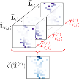
(b) The computation of $\widetilde{\mathcal{C}}(\widetilde{\mathbf{T}}^{(r)})$.

Figure 1: (a) An illustration of our Spar-GW. The non-zero elements of each matrix are labeled with colors. The arrows between $\widetilde{\mathbf{T}}^{(r)}$’s are applied when using the proximal gradient algorithm. (b) An illustration of the computation of $\widetilde{\mathcal{C}}(\widetilde{\mathbf{T}}^{(r)})$ in the $r$-th iteration.

3.2 Proposed algorithm

Let $\mathbf{P}$ be the sampling probability matrix such that the $(i,j)$-th element equals the $p_{ij}$ in (5). Given $\mathbf{P}$, we first construct the index set $\mathcal{S}$ by sampling $s$ pairs of indices, and then, build $s$ matrices $\{\widetilde{\mathbf{L}}_{i\cdot j\cdot}\}_{(i,j)\in\mathcal{S}}$, whose elements are

$$\widetilde{L}_{ii^{\prime}jj^{\prime}}=\begin{cases}\mathcal{L}(C^{X}_{ii^{\prime}},C^{Y}_{jj^{\prime}})&\text{ if }(i^{\prime},j^{\prime})\in\mathcal{S}\\ 0&\text{ otherwise. }\end{cases}\quad\text{ for }(i,j)\in\mathcal{S}.$$ (6)

As shown in Figure 1(b), in the $r$-th iteration, we construct a sparse coupling matrix $\widetilde{\mathbf{T}}^{(r)}$, with $\widetilde{T}^{(r)}_{ij}=0$ if $(i,j)\notin\mathcal{S}$, and compute the sparse cost matrix $\widetilde{\mathcal{C}}(\widetilde{\mathbf{T}}^{(r)})=\sum_{(i,j)\in\mathcal{S}}\widetilde{\mathbf{L}}_{i\cdot j\cdot}\widetilde{T}^{(r)}_{ij}$. Accordingly, we derive the sparse kernel matrix $\widetilde{\mathbf{K}}^{(r)}$ with non-zero elements

$$\widetilde{K}^{(r)}_{ij}=\exp(-\widetilde{\mathcal{C}}_{ij}/\varepsilon)\widetilde{T}^{(r)}_{ij}/(sp_{ij})~{}~{}\text{or}~{}~{}\exp(-\widetilde{\mathcal{C}}_{ij}/\varepsilon)/(sp_{ij})$$

only for $(i,j)\in\mathcal{S}$, where the adjustment factor $sp_{ij}$ ensures the unbiasedness of the estimation. We then calculate the coupling matrix $\widetilde{\mathbf{T}}^{(r+1)}$ via applying the Sinkhorn-scaling algorithm to the sparse $\widetilde{\mathbf{T}}^{(r)}$ and $\widetilde{\mathbf{K}}^{(r)}$. Algorithm 2 summarizes the Spar-GW algorithm.

Algorithm 2 Spar-GW algorithm

1:Input: Sample distributions $\bm{a},\bm{b}$, relation matrices $\mathbf{C}^{X},\mathbf{C}^{Y}$, ground cost function $\mathcal{L}$, regularization parameter $\varepsilon$, number of selected elements $s$, number of outer/inner iterations $R$, $H$

2:Construct the sampling probability $\mathbf{P}$ defined by (5) $O(mn)$

3:Generate an i.i.d. subsample of size $s$ using $\mathbf{P}$, let $\mathcal{S}=\{(i_{l}^{\prime},j_{l}^{\prime})\}_{l=1}^{s}$ be the index set

4:Initialize $\widetilde{\mathbf{T}}^{(0)}=\mathbf{0}_{m\times n}$ and $\widetilde{T}_{ij}^{(0)}=a_{i}b_{j}$ if $(i,j)\in\mathcal{S}$

5:For $r=0\textbf{ to }R-1$:

6:  Construct a sparse kernel matrix: $O(s^{2})$ a) Compute $\widetilde{\mathcal{C}}(\widetilde{\mathbf{T}}^{(r)})=\sum_{(i,j)\in\mathcal{S}}\widetilde{\mathbf{L}}_{i\cdot j\cdot}\widetilde{T}_{ij}^{(r)}$ using (6), and replace its 0’s at $\mathcal{S}$ with $\infty$’s b) $\widetilde{\mathbf{K}}^{(r)}=\begin{cases}\exp(-\frac{\widetilde{\mathcal{C}}(\widetilde{\mathbf{T}}^{(r)})}{\varepsilon})\odot\widetilde{\mathbf{T}}^{(r)}\oslash(s\mathbf{P})&\text{ if }\mathcal{R}(\mathbf{T})=\text{KL}(\mathbf{T}\|\mathbf{T}^{(r)})\\ \exp(-\frac{\widetilde{\mathcal{C}}(\widetilde{\mathbf{T}}^{(r)})}{\varepsilon})\oslash(s\mathbf{P})&\text{ if }\mathcal{R}(\mathbf{T})=H(\mathbf{T})\end{cases}$

7:  Sinkhorn-scaling (with sparse inputs): $\widetilde{\mathbf{T}}^{(r+1)}=\textsc{Sinkhorn}(\bm{a},\bm{b},\widetilde{\mathbf{K}}^{(r)},H)$ $O(Hs)$

8:Output: $\widehat{\operatorname{GW}}=\sum_{(i,j)\cap(i^{\prime},j^{\prime})\in\mathcal{S}}\mathcal{L}\left(C_{ii^{\prime}}^{X},C_{jj^{\prime}}^{Y}\right)\widetilde{T}^{(R)}_{ij}\widetilde{T}^{(R)}_{i^{\prime}j^{\prime}}$ $O(s^{2})$

Computational cost. Generating the sampling probability matrix $\mathbf{P}$ requires $O(mn)$ time. In each iteration, calculating $\widetilde{\mathcal{C}}(\widetilde{\mathbf{T}}^{(r)})$ involves the summation of $s$ matrices, and each of them contains only $s$ non-zero elements, resulting in $O(s^{2})$ time. For Step 7, the Sinkhorn-scaling algorithm requires $O(Hs)$ time by using sparse matrix multiplications. Calculating GW distance using the sparse $\widetilde{\mathbf{T}}^{(R)}$ requires $O(s^{2})$ operations. Therefore, for Algorithm 2, its overall time complexity is $O(mn+Rs^{2}+RHs+s^{2})$, which becomes $O(mn+s^{2})$ when $R$ and $H$ are constants, and its memory cost is $O(mn)$. When $m=O(n)$, we obtain the complexity shown in Table 1.

Applicability for entropic GW distance and fused GW distance. As shown in Algorithm 2, our algorithm can approximate the entropic GW distance as well. Moreover, it is natural to extend the algorithm to approximate the fused Gromov-Wasserstein (FGW) distance (Titouan et al., 2019a, ; Vayer et al.,, 2020). In particular, when computing the FGW distance, the cost matrix $\mathcal{C}(\mathbf{T})$ takes the direct comparison among the samples into account, and our importance sparsification mechanism is still applicable. Details for the modified algorithm are relegated to Appendix.

4 Theoretical results

This section shows the convergence and consistency of $\widehat{\text{GW}}$ obtained by Algorithm 2 under $\mathcal{R}(\mathbf{T})=H(\mathbf{T})$. To ease the conversation, we focus on the case that $m=n$, and the extension to unequal cases is straightforward. Let $(\mathbf{T},\mathbf{T}^{\prime})\in\Pi^{2}(\bm{a},\bm{b})$. We define

$$\mathcal{E}(\mathbf{T},\mathbf{T}^{\prime}):=\sideset{}{{}_{i,i^{\prime},j,j^{\prime}}}{\sum}\mathcal{L}\left(C_{ii^{\prime}}^{X},C_{jj^{\prime}}^{Y}\right)T_{ij}T_{i^{\prime}j^{\prime}}^{\prime},\quad G(\mathbf{T}):=\mathcal{E}(\mathbf{T},\mathbf{T})-\sideset{}{{}_{\mathbf{T}^{\prime}\in\Pi(\bm{a},\bm{b})}}{\min}\mathcal{E}(\mathbf{T},\mathbf{T}^{\prime}).$$

For notation simplicity, we overload $\mathcal{E}(\mathbf{T},\mathbf{T})$ as $\mathcal{E}(\mathbf{T})$. Following Kerdoncuff et al., (2021), our goal is to provide a guarantee on the convergence of $G(\mathbf{T})$, because $\mathbf{T}$ is a stationary point of $\mathcal{E}(\mathbf{T})$ if and only if $G(\mathbf{T})=0$ (Reddi et al.,, 2016). In addition, we define $\accentset{{\cc@style\underline{\mskip 10.0mu}}}{\mathbf{K}}^{(r)}=\exp(-\mathcal{C}(\widetilde{\mathbf{T}}^{(r)})/\varepsilon)$, which is the unsampled counterpart to $\widetilde{\mathbf{K}}^{(r)}$ at the $r$-th iteration. Consider the following regularity conditions.

• The relation matrices $\mathbf{C}^{X},\mathbf{C}^{Y}$ are symmetric;

• The ground cost is bounded, i.e., $0\leq\mathcal{L}(C_{ii^{\prime}}^{X},C_{jj^{\prime}}^{Y})\leq 2B$ for a constant $B>0$;

• $\|\accentset{{\cc@style\underline{\mskip 10.0mu}}}{\mathbf{K}}^{(r)}\|_{2}\geq n^{\alpha}/c_{1}$ for constants $1/2<\alpha\leq 1$ and $c_{1}>0$, and the condition number of $\accentset{{\cc@style\underline{\mskip 10.0mu}}}{\mathbf{K}}^{(r)}$ is positive and bounded by $c_{2}>0$, for any $r\leq R-1$;

• $p_{ij}\geq{c_{3}}/{n^{2}}$ for a constant $c_{3}>0$;

• $s\geq c_{4}n^{3-2\alpha}\log^{4}(n)$ for constants $c_{4}=8\log^{4}(2)/(c_{3}\log^{4}(1+\epsilon))$ and $\epsilon>0$.

Conditions (H.1)–(H.3) are natural. Condition (H.4) indicates that the sampling probabilities could not be too small, requiring $p_{ij}$ to be at the order of $O(1/n^{2})$. The order can always be satisfied by linear interpolating between the proposed sampling probability and the uniform sampling probability. Such a shrinkage strategy is commonly used in subsampling literature (Ma et al.,, 2015; Yu et al.,, 2022). Condition (H.5) requires $s$ to be large enough. For a general case that $\|\accentset{{\cc@style\underline{\mskip 10.0mu}}}{\mathbf{K}}^{(r)}\|_{2}=O(n)$, i.e., $\alpha=1$, condition (H.5) can be achieved when $s=O(n^{1+\delta})$ for an arbitrary small $\delta>0$. Such order indicates we only need to compute around $n^{2}$ elements from the entire tensor that contains $n^{4}$ elements.

We now provide our main convergence result, whose proofs are provided in Appendix.

Theorem 1.

Under the conditions (H.1)–(H.5), assume that $R\exp\left(-{16}\log^{4}(n)/{\epsilon^{4}}\right)\to 0$ for some $\epsilon>0$, and $n>76$. The following bound holds in probability

$$G({\widetilde{\mathbf{T}}^{(R-1)}})\leq\frac{\mathcal{E}(\widetilde{\mathbf{T}}^{(R)})-\mathcal{E}(\widetilde{\mathbf{T}}^{(R-1)})}{2}+6\sqrt{2}\varepsilon{(2+\epsilon)}c_{1}c_{2}\sqrt{\frac{n^{3-2\alpha}}{c_{3}s}}+\varepsilon\log(n)+Bn^{2}\|\widetilde{\mathbf{T}}^{(R)}-\widetilde{\mathbf{T}}^{(R-1)}\|_{F}^{2}.$$ (7)

Consider the upper bound in Theorem 1. The second term on the right-hand side of (7) results from importance sparsification. Under the common condition that $\alpha=1$, it tends to zero when $s=O(n^{1+\delta})$ as $n\to\infty$. The third term $\varepsilon\log(n)$ is caused by the regularization mechanism, which goes to zero when $\varepsilon=o(\log^{-1}(n))$. The remaining terms are due to the iterative scheme in Algorithm 2. Theorem 1 indicates that the estimation error of the proposed estimator decreases when the regularization parameter $\varepsilon$ decreases or the subsample size $s$ increases. We provide the following corollary to show the consistency of the proposed estimator.

Corollary 1.

Suppose the conditions of Theorem 1 hold with $\alpha=1$. Further suppose Algorithm 2 converges with $\|\widetilde{\mathbf{T}}^{(R)}-\widetilde{\mathbf{T}}^{(R-1)}\|_{F}\leq c_{5}/n^{3/2+\eta}$ for some $c_{5},\eta>0$. When $s=O(n^{1+\delta})$ for any $\delta>0$ and $\varepsilon=o(\log^{-1}(n))$, $G({\widetilde{\mathbf{T}}^{(R-1)}})\to 0$ in probability, as $n\rightarrow\infty$.

The local stationary convergence of Algorithm 2 implies $\widetilde{\mathbf{T}}^{(R)}$ and $\widetilde{\mathbf{T}}^{(R-1)}$ will get closer and closer with the increase of $R$. Therefore, for any given $n$, we can set the assumption $||\widetilde{\mathbf{T}}^{(R)}-\widetilde{\mathbf{T}}^{(R-1)}||_{F}\leq c_{5}/n^{3/2+\eta}$ as the stopping criterion, which can be naturally satisfied for a relatively large $R$.

5 Importance sparsification for UGW distance

5.1 Unbalanced GW distance

In this section, we extend the Spar-GW algorithm to approximate the unbalanced Gromov-Wasserstein (UGW) distance. Similar to the unbalanced optimal transport (UOT) (Liero et al.,, 2016; Chizat et al., 2018c, ; Chizat et al., 2018b, ; Chizat et al., 2018a, ), UGW distance is able to compare metric-measure spaces endowed with arbitrary positive distributions $\bm{a}\in\mathbb{R}^{m}_{+},\bm{b}\in\mathbb{R}^{n}_{+}$ (Séjourné et al.,, 2021; Kawano and Mason,, 2021; Luo et al.,, 2022). Following the definition in Séjourné et al., (2021), UGW distance relaxes the marginal constraints via the quadratic KL-divergence $\mathrm{KL}^{\otimes}(\mu\|\nu)=\mathrm{KL}(\mu\otimes\mu\|\nu\otimes\nu)$, where $\mu\otimes\nu$ is the tensor product measure defined by $d(\mu\otimes\nu)(x,y)=d\mu(x)d\nu(y)$. In particular, UGW distance takes the form

$$\operatorname{UGW}\left((\mathbf{C}^{X},\bm{a}),(\mathbf{C}^{Y},\bm{b})\right)$$

$$:= \sideset{}{{}_{\mathbf{T}\in\mathbb{R}_{+}^{m\times n}}}{\min}\langle\mathcal{L}(\mathbf{C}^{X},\mathbf{C}^{Y})\otimes\mathbf{T},\mathbf{T}\rangle+\lambda\mathrm{KL}^{\otimes}(\mathbf{T}\mathbf{1}_{n}\|\bm{a})+\lambda\mathrm{KL}^{\otimes}(\mathbf{T}^{\top}\mathbf{1}_{m}\|\bm{b})$$

$$= \sideset{}{{}_{\mathbf{T}\in\mathbb{R}_{+}^{m\times n}}}{\min}\langle\mathcal{C}_{\text{un}}(\mathbf{T}),\mathbf{T}\rangle+\lambda m(\mathbf{T})\mathrm{KL}(\mathbf{T}\mathbf{1}_{n}\|\bm{a})+\lambda m(\mathbf{T})\mathrm{KL}(\mathbf{T}^{\top}\mathbf{1}_{m}\|\bm{b}).$$

Here, $m(\mathbf{T})=\sum_{i,j}T_{ij}$ is the total mass of $\mathbf{T}$, $\mathcal{C}_{\text{un}}(\mathbf{T}):=\mathcal{L}(\mathbf{C}^{X},\mathbf{C}^{Y})\otimes\mathbf{T}+E(\mathbf{T})$ is the cost matrix with $E(\mathbf{T}):=\lambda\sum_{i}\log(\sum_{j}T_{ij}/a_{i})\sum_{j}T_{ij}+\lambda\sum_{j}\log(\sum_{i}T_{ij}/b_{j})\sum_{i}T_{ij},$ and $\lambda>0$ is the marginal regularization parameter balancing the trade-off between mass transportation and mass variation. Note that when $\bm{a}\in\Delta^{m-1}$ and $\bm{b}\in\Delta^{n-1}$, UGW distance degenerates to the classical GW distance as $\lambda\to\infty$.

5.2 Proposed algorithm

To approximate the UGW distance, we update the coupling matrix via proximal gradient algorithm (PGA) by adding a Bregman proximal term (Xie et al.,, 2020; Xu et al., 2019b, ; Kerdoncuff et al.,, 2021). Specifically, $\mathbf{T}$ is updated as

$$\mathbf{T}^{(r+1)}=\operatorname{argmin}_{\mathbf{T}\in\mathbb{R}_{+}^{m\times n}} \langle\mathcal{C}_{\text{un}}(\mathbf{T}^{(r)}),\mathbf{T}\rangle+\lambda m(\mathbf{T}^{(r)})\mathrm{KL}(\mathbf{T}\mathbf{1}_{n}\|\bm{a})$$

$$+\lambda m(\mathbf{T}^{(r)})\mathrm{KL}(\mathbf{T}^{\top}\mathbf{1}_{m}\|\bm{b})+\varepsilon m(\mathbf{T}^{(r)})\mathrm{KL}(\mathbf{T}\|\mathbf{T}^{(r)}).$$ (8)

The subproblem (8) can be solved using unbalanced Sinkhorn-scaling algorithm (Chizat et al., 2018b, ; Pham et al.,, 2020) with the kernel matrix $\mathbf{K}=\exp\{-\mathcal{C}_{\text{un}}(\mathbf{T}^{(r)}))/(\varepsilon m(\mathbf{T}^{(r)}))\}\odot\mathbf{T}^{(r)}$; see Step 9 in Algorithm 3 for details. Now the convergent scaling vectors $\bm{u}\in\mathbb{R}^{m}_{+},\bm{v}\in\mathbb{R}^{n}_{+}$ satisfies that

$$(u_{i})^{\frac{\lambda+\varepsilon}{\lambda}}\left(\sum\nolimits_{j}K_{ij}v_{j}\right)=a_{i}\quad\quad\text{and}\quad\quad(v_{j})^{\frac{\lambda+\varepsilon}{\lambda}}\left(\sum\nolimits_{i}K_{ij}u_{i}\right)=b_{j}.$$

As a result, it holds that

$$(u_{i})^{\frac{\lambda+\varepsilon}{\lambda}}K_{ij}v_{j}\leq a_{i},\quad u_{i}K_{ij}(v_{j})^{\frac{\lambda+\varepsilon}{\lambda}}\leq b_{j}\quad\Rightarrow\quad(u_{i})^{\frac{2\lambda+\varepsilon}{\lambda}}K_{ij}^{2}(v_{j})^{\frac{2\lambda+\varepsilon}{\lambda}}\leq a_{i}b_{j},$$

which follows that $T^{\ast}_{ij}=u_{i}K_{ij}v_{j}\leq\left(a_{i}b_{j}\right)^{\frac{\lambda}{2\lambda+\varepsilon}}K_{ij}^{\frac{\varepsilon}{2\lambda+\varepsilon}}$. Such an inequality motivates us to sample with probability

$$p_{ij}=\frac{(a_{i}b_{j})^{\frac{\lambda}{2\lambda+\varepsilon}}K_{ij}^{\frac{\varepsilon}{2\lambda+\varepsilon}}}{\sum_{i,j}(a_{i}b_{j})^{\frac{\lambda}{2\lambda+\varepsilon}}K_{ij}^{\frac{\varepsilon}{2\lambda+\varepsilon}}},\quad 1\leq i\leq m,\quad 1\leq j\leq n.$$ (9)

Unfortunately, such a probability involves the kernel matrix $\mathbf{K}$, which requires the unknown coupling matrix $\mathbf{T}$. To bypass the obstacle, we propose to replace the unknown $\mathbf{T}$ with the initial value $\widetilde{\mathbf{T}}^{(0)}=\bm{a}\bm{b}^{\top}/\sqrt{m(\bm{a})m(\bm{b})}$, where $m(\bm{a})=\sum_{i}a_{i}$ and $m(\bm{b})=\sum_{j}b_{j}$ are the total mass of $\bm{a}$ and $\bm{b}$, respectively. Algorithm 3 details the proposed Spar-UGW algorithm for approximating UGW distances. Note that when $m(\bm{a})=m(\bm{b})$ and $\lambda\to\infty$, Spar-UGW degenerates to Spar-GW. Such an observation is consistent with the relationship between GW and UGW.

Algorithm 3 Spar-UGW algorithm

1:Input: Sample distributions $\bm{a},\bm{b}$, relation matrices $\mathbf{C}^{X},\mathbf{C}^{Y}$, ground cost function $\mathcal{L}$, regularization parameters $\lambda,\varepsilon$, number of selected elements $s$, number of outer/inner iterations $R$, $H$

2:Initialize $\widetilde{\mathbf{T}}^{(0)}=\bm{a}\bm{b}^{\top}/\sqrt{m(\bm{a})m(\bm{b})}$

3:$\mathbf{K}=\exp\{-\mathcal{C}_{\text{un}}(\widetilde{\mathbf{T}}^{(0)})/(\varepsilon m(\widetilde{\mathbf{T}}^{(0)}))\}\odot\widetilde{\mathbf{T}}^{(0)}$ $O(m^{2}n^{2})$ or $O(mn)$

4:Construct the sampling probability $\mathbf{P}$ defined by (9) $O(mn)$

5:Generate an i.i.d. subsample of size $s$ using $\mathbf{P}$, let $\mathcal{S}=\{(i_{l}^{\prime},j_{l}^{\prime})\}_{l=1}^{s}$ be the index set

6:For $r=0\textbf{ to }R-1$:

7:  $\bar{\varepsilon}=\varepsilon m(\widetilde{\mathbf{T}}^{(r)}),\bar{\lambda}=\lambda m(\widetilde{\mathbf{T}}^{(r)})$

8:  Construct a sparse kernel matrix: $O(s^{2})$ a) Compute the cost matrix $\widetilde{\mathcal{C}}_{\text{un}}(\widetilde{\mathbf{T}}^{(r)})=\sum_{(i,j)\in\mathcal{S}}\widetilde{\mathbf{L}}_{i\cdot j\cdot}\widetilde{T}_{ij}^{(r)}+E(\widetilde{\mathbf{T}}^{(r)})$ using formula (6) and replace its 0’s at $\mathcal{S}$ with $\infty$’s b) $\widetilde{\mathbf{K}}^{(r)}=\exp(-\frac{\widetilde{\mathcal{C}}_{\text{un}}(\widetilde{\mathbf{T}}^{(r)})}{\bar{\varepsilon}})\odot\widetilde{\mathbf{T}}^{(r)}\oslash(s\mathbf{P})$

9:  Unbalanced Sinkhorn-scaling: $\widetilde{\mathbf{T}}^{(r+1)}=\textsc{Sinkhorn}_{\textsc{UOT}}(\bm{a},\bm{b},\widetilde{\mathbf{K}}^{(r)},\bar{\lambda},\bar{\varepsilon},H)$ $O(Hs)$ a) Initialize $\bm{u}^{(0)}=\mathbf{1}_{m},\bm{v}^{(0)}=\mathbf{1}_{n}$ b) For $h=0\textbf{ to }H-1$: $\bm{u}^{(h+1)}=(\bm{a}\oslash(\widetilde{\mathbf{K}}^{(r)}\bm{v}^{(h)}))^{\bar{\lambda}/(\bar{\lambda}+\bar{\varepsilon})}$,  $\bm{v}^{(h+1)}=(\bm{b}\oslash(\widetilde{\mathbf{K}}^{{}^{(r)}\top}\bm{u}^{(h+1)}))^{\bar{\lambda}/(\bar{\lambda}+\bar{\varepsilon})}$ c) $\widetilde{\mathbf{T}}^{(r+1)}=\operatorname{diag}(\bm{u}^{(H)})\widetilde{\mathbf{K}}^{(r)}\operatorname{diag}(\bm{v}^{(H)})$

10:  $\widetilde{\mathbf{T}}^{(r+1)}=\sqrt{m(\widetilde{\mathbf{T}}^{(r)})/m(\widetilde{\mathbf{T}}^{(r+1)})}\cdot\widetilde{\mathbf{T}}^{(r+1)}$

11:Output: $\widehat{\operatorname{UGW}}=\langle\mathcal{L}(\mathbf{C}^{X},\mathbf{C}^{Y})\otimes\widetilde{\mathbf{T}}^{(R)},\widetilde{\mathbf{T}}^{(R)}\rangle+\lambda\mathrm{KL}^{\otimes}(\widetilde{\mathbf{T}}^{(R)}\mathbf{1}_{n}\|\bm{a})+\lambda\mathrm{KL}^{\otimes}(\widetilde{\mathbf{T}}^{(R)\top}\mathbf{1}_{m}\|\bm{b})$ $O(s^{2})$

Computational cost. In Algorithm 3, although calculating $\mathbf{K}$ in Step 3 requires $O(m^{2}n^{2})$ time, we only need to calculate it once. Moreover, when $\mathcal{L}$ is decomposable, the complexity of calculating $\mathbf{K}$ can be reduced to $O(mn)$ by utilizing the fact that $\mathbf{T}^{(0)}$ is a rank-one matrix. Therefore, the total time complexity of Spar-UGW is $O(mn+s^{2})$ when $R$ and $H$ are constants, and $\mathcal{L}$ is decomposable.

6 Experiments

In this section, we evaluate the performance of Spar-GW and its variants in both distance estimation and graph analysis.

6.1 Synthetic data analysis

6.1.1 Approximation of GW and UGW distances

We compare the proposed Spar-GW with main competitors including: (i) EGW, Algorithm 1 with entropic regularization (Peyré et al.,, 2016); (ii) PGA-GW, Algorithm 1 with proximal regularization (Xu et al., 2019b, ); (iii) EMD-GW, i.e., EGW with $\varepsilon=0$, but replacing Sinkhorn-scaling algorithm in EGW with the solver for unregularized OT problems (Bonneel et al.,, 2011); (iv) S-GWL (Xu et al., 2019a, ), adapted for arbitrary ground cost following Kerdoncuff et al., (2021); (v) LR-GW, the quadratic approach in Scetbon et al., (2022); (vi) SaGroW (Kerdoncuff et al.,, 2021). Other methods in Table 1, i.e., Sliced GW (Titouan et al., 2019b, ), AE (Sato et al.,, 2020) and FlowAlign (Le et al.,, 2021), are not included as they fail to approximate the original GW distance. We adopted the proximal term, i.e., KL-divergence, as $\mathcal{R}(\mathbf{T})$ in SaGroW and Spar-GW. The other choice of regularization term yields similar results. The regularization parameter $\varepsilon$ is chosen among $\{1,10^{-1},10^{-2},10^{-3}\}$ and the result with the smallest distance w.r.t. each method is presented. For LR-GW, the non-negative rank of the coupling matrix is set to $\lceil n/20\rceil$. For Spar-GW and Spar-UGW, we set the subsample size $s=16n$. For a fair comparison, we set the subsample size $s^{\prime}=s^{2}/n^{2}$ for SaGroW to ensure that it has the same sampling budget (i.e., samples the same number of elements) to Spar-GW (or Spar-UGW). Other parameters of the methods mentioned above are set by default. To take into account the randomness of sampling-based methods, i.e., SaGroW, Spar-GW, and Spar-UGW, their estimations are averaged over ten runs. All the experiments are performed on a server with 8-core CPUs and 30GB RAM.

We consider two popular synthetic datasets called Moon following Séjourné et al., (2021); Muzellec et al., (2020), and Graph following Xu et al., 2019b ; Xu et al., 2019a . We also consider two other widely-used datasets including the case where the source and target are distributed in heterogeneous spaces. The results have a similar pattern to those of Moon and are relegated to Appendix. Specifically, for the Moon dataset, marginals are two Gaussian distributions, $N(n/3,n/20)$ and $N(n/2,n/20)$, supported on $n$ points in $\mathbb{R}^{2}$. The source and target supported points are respectively generated from two interleaving half circles by sklearn toolbox (Pedregosa et al.,, 2011). The matrices $\mathbf{C}^{X},\mathbf{C}^{Y}$ are defined using pairwise Euclidean distances in $\mathbb{R}^{2}$. For the Graph dataset, we first generate one graph with $n$ nodes and power-law degree distribution from NetworkX library (Hagberg et al.,, 2008), and then generate the other graph by adding extra edges randomly with probability 0.2 on the first one. Their degree distributions are used as two marginals, and the adjacency matrix of each graph is used as $\mathbf{C}^{X},\mathbf{C}^{Y}$. Both $\ell_{1}$ and $\ell_{2}$ losses are considered for the ground cost. LR-GW is only capable of the $\ell_{2}$ loss, and thus its result w.r.t. the $\ell_{1}$ loss is omitted. To compare the estimation accuracy w.r.t. different methods, we take PGA-GW as a benchmark and calculate the absolute error between its estimation and other estimations of GW distance.

Figure 2: Comparison on estimation error (Top) and CPU time (Bottom). The mean and standard deviation are reported for sampling-based methods.

Figure 2 shows the estimation error (top row) and the CPU time (bottom row) versus increasing sample size $n$. We observe that the proposed Spar-GW method yields almost the smallest estimation error for the Moon dataset and reasonable errors for the Graph dataset. Such a difference is because Gaussian distributions in Moon are more concentrated and thus are easier to sketch by subsamples; while the structure of graphs in Graph is more complicated, and the transportation between their degree distributions is also more difficult to approximate by the subsampling technique. As for computational efficiency, Spar-GW requires less CPU time than most of the competitors, and such an advantage is more obvious for the indecomposable $\ell_{1}$ loss. These observations indicate Spar-GW is capable of dealing with large-scale GW problems with arbitrary ground cost.

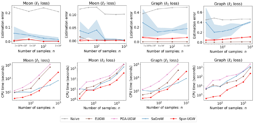
Figure 3: Comparison on estimation error (Top) and CPU time (Bottom) w.r.t. UGW distance. The mean and standard deviation are reported for sampling-based methods.

For unbalanced problems, we set the total mass of $\bm{a},\bm{b}$ to be units and the marginal relaxation parameter to be $\lambda=1$. We compare Spar-UGW with: (i) Naive transport plan $\mathbf{T}=\bm{a}\bm{b}^{\top}$; (ii) EUGW, entropic regularization in Séjourné et al., (2021); (iii) PGA-UGW; (iv) SaGroW, adapted for unbalanced problems. We calculate the estimation error w.r.t. the PGA-UGW benchmark. Other settings are the same as the aforementioned. From Fig. 3, we observe that Spar-UGW consistently achieves the best accuracy for the former dataset and a relatively small estimation error for the latter one, requiring the least amount of time for the $\ell_{2}$ loss. Although the computational cost of Spar-UGW becomes more considerable for the indecomposable $\ell_{1}$ loss, it still computes much faster than the classical EUGW and PGA-UGW methods.

6.1.2 Sensitivity analysis

We now show that our method is robust to hyperparameters by analyzing its sensitivity to the subsample size $s$ and the regularization parameter $\varepsilon$. Specifically, for synthetic datasets with fixed sample size $n=200$, the hyperparameters are considered among $s\in\{2^{1},2^{2},\ldots,2^{5}\}\times n$ and $\varepsilon\in\{5^{0},5^{-1},\ldots,5^{-4}\}$.

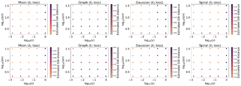
(a) Sensitivity on the estimated GW distance.

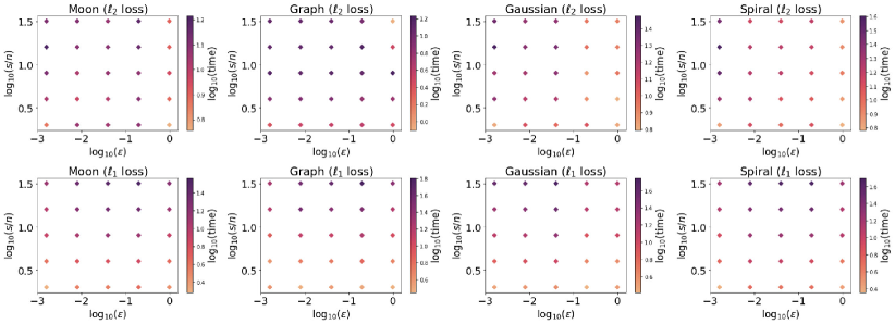
(b) Sensitivity on the CPU time.

Figure 4: Impact of the subsample size $s$ and the regularization parameter $\varepsilon$ for Spar-GW on the GW distance estimation (panel (a)) and computational time (panel (b)). The mean over ten runs are reported.

From the results in Fig. 4, we find that a large number of selected elements $s$ and/or a small value of $\varepsilon$ is associated with a small GW distance estimation and a long CPU time. Such a finding is consistent with our theoretical results. We also observe that Spar-GW can yield a satisfactory estimation for a large range of hyperparameters. More precisely, as long as $s=O(n)$ and $\varepsilon$ is not too large, the estimated GW distance is approximately in the same order, which implies Spar-GW is not sensitive to hyperparameters and can cover a wide range of trade-offs between accuracy and speed. This observation supports the key assumption that only a few important elements in kernel and coupling matrices are required to approximate the GW distance effectively. Moreover, our method is largely free from numerical instability because $\varepsilon$ need not be extremely small, which is in good agreement with the statements in Xie et al., (2020); Xu et al., 2019b .

6.2 Real-world applications

We consider two applications, graph clustering and graph classification, to demonstrate the effectiveness of our method in applications. Six widely-used benchmark datasets are considered: BZR, COX2 (Sutherland et al.,, 2003), CUNEIFORM (Kriege et al.,, 2018), SYNTHETIC (Feragen et al.,, 2013) with vector node attributes; FIRSTMM_DB (Neumann et al.,, 2013) with discrete attributes; and IMDB-B (Yanardag and Vishwanathan,, 2015) with no attributes. All these datasets are available in PyTorch Geometric library (Fey and Lenssen,, 2019). Given $N$ graphs, we first compute the pairwise GW distance matrix $\mathbf{D}\in\mathbb{R}^{N\times N}$ and then construct the similarity matrix $\mathbf{S}=\exp(-\mathbf{D}/\gamma)$ for $\gamma>0$. For methods that can directly extend to approximate the fused GW (FGW) distance, including EGW, PGA-GW, EMD-GW, SaGroW, and Spar-GW, we obtain the pairwise FGW distance matrix when the graphs have attributes. We set the trade-off parameter $\alpha=0.6$. Empirical results show the performance is not sensitive to $\alpha$. For the graph clustering task, we apply spectral clustering to the similarity matrix. We replicate the experiment ten times with different random initialization and assess the clustering performance by average Rand index (RI) (Rand,, 1971). For the classification task, we train a classifier based on kernel SVM using the similarity matrix and test the classifier via nested ten-fold cross-validation following Titouan et al., 2019a . The performance is evaluated by average classification accuracy. To examine the effect of different loss functions, we consider both $\ell_{1}$ loss and $\ell_{2}$ loss for AE, SaGroW, and Spar-GW. Other methods are mainly designed for the decomposable loss, and thus only the $\ell_{2}$ loss is implemented. For all methods, $\gamma$ is cross validated within $\{2^{-10},2^{-9},\ldots,2^{10}\}$. Other settings are the same as those in the previous section.

Table 2: Comparison on clustering performance w.r.t. RI (%).

Dataset	SYNTHETIC	BZR	Cuneiform	COX2	FIRSTMM_DB	IMDB-B
# graphs: $N$	300	405	267	467	41	1000
Ave. # nodes: $n$	100.00	35.75	21.27	41.22	1377.27	19.77
Subsample size: $s$	$2^{5}\times n$	$2^{3}\times n$	$2^{3}\times n$	$2^{3}\times n$	$2^{7}\times n$	$2^{3}\times n$
EGW	100.00±0.00	67.18±0.44	94.90±0.08	64.81±0.58	92.51±0.15	50.79±0.00
S-GWL	100.00±0.00	66.84±0.73	94.32±0.07	65.02±0.23	81.42±0.16	51.30±0.00
LR-GW	50.13±0.02	65.34±4.31	26.47±0.57	64.99±0.10	45.93±3.14	51.54±0.01
AE ($\ell_{2}$ loss)	50.17±0.59	67.04±0.00	82.51±3.24	62.36±0.03	84.63±0.00	50.79±0.03
AE ($\ell_{1}$ loss)	50.17±0.59	67.04±0.00	82.64±3.22	62.36±0.00	84.67±0.11	50.79±0.03
SaGroW ($\ell_{2}$ loss)	52.41±0.00	67.24±0.26	94.56±0.20	65.94±0.92	92.07±0.00	50.45±0.00
SaGroW ($\ell_{1}$ loss)	54.15±0.19	67.33±0.47	94.54±0.14	65.97±1.03	92.09±0.35	50.45±0.00
Spar-GW ($\ell_{2}$ loss)	98.67±0.00	68.22±0.00	94.66±0.05	65.54±0.00	92.24±0.30	50.82±0.00
Spar-GW ($\ell_{1}$ loss)	98.67±0.00	68.22±0.00	94.64±0.06	66.29±1.09	92.41±0.33	50.82±0.00

• The top-3 results of each dataset are in bold, and the best result is in italics.

Table 3: Comparison on classification performance w.r.t. accuracy (%).

Dataset	SYNTHETIC	BZR	Cuneiform	COX2	FIRSTMM_DB	IMDB-B
EGW	100.00±0.00	85.92±0.50	25.66±2.01	80.21±0.59	53.75±2.24	66.01±0.64
S-GWL	100.00±0.00	87.67±0.41	9.05±1.13	78.23±0.22	17.50±4.03	64.54±0.55
LR-GW	55.83±1.46	79.12±0.34	3.77±0.46	78.06±0.20	15.25±3.05	58.47±0.35
AE ($\ell_{2}$ loss)	43.47±1.18	81.48±0.20	4.90±0.67	78.11±0.19	10.00±3.49	62.98±0.40
AE ($\ell_{1}$ loss)	44.73±1.69	81.65±0.34	5.28±0.60	78.19±0.25	14.50±3.72	63.54±0.49
SaGroW ($\ell_{2}$ loss)	66.33±1.52	79.47±0.32	17.84±1.43	78.06±0.37	47.50±4.10	67.40±0.37
SaGroW ($\ell_{1}$ loss)	68.97±1.31	80.17±0.76	16.98±1.44	78.27±0.54	50.00±2.79	67.69±0.55
Spar-GW ($\ell_{2}$ loss)	98.79±0.16	83.65±0.22	18.87±0.99	78.92±0.11	54.25±3.17	66.70±0.46
Spar-GW ($\ell_{1}$ loss)	99.00±0.22	84.19±0.33	22.26±1.35	78.49±0.69	62.50±3.81	67.00±0.41

• The top-3 results of each dataset are in bold, and the best result is in italics.

Tables 2 and 3 report the average RI and average classification accuracy with the corresponding standard deviation, respectively. PGA-GW and EMD-GW are excluded for clarity as their results are similar to EGW. Sliced GW and FlowAlign are also not included since they cannot handle graphs. From Tables 2 and 3, we observe the proposed Spar-GW approach is superior or at least comparable to other methods in all cases. We also observe the Spar-GW with $\ell_{1}$ cost almost consistently outperforms the one with $\ell_{2}$ cost. This observation is consistent with the observation in Kerdoncuff et al., (2021), which stated that the $\ell_{1}$ cost tends to yield better performance than the $\ell_{2}$ cost in graphical data analysis. Such observation also justifies the essence of developing a computational tool that can handle arbitrary ground costs in GW distance approximation.

Considering the CPU time, Spar-GW computes much faster than EGW, S-GWL, and AE when the number of nodes is relatively large. Take the FIRSTMM_DB dataset as an example, in which each graph has an average of 1,377 nodes, the average CPU time for these methods are 414.82s (EGW), 1059.95s (S-GWL), 22.41s (LR-GW), 501.06s/530.12s (AE under $\ell_{2}$ loss/$\ell_{1}$ loss), 196.18s/189.57s (SaGroW under $\ell_{2}$ loss/$\ell_{1}$ loss), and 82.45s/147.33s (Spar-GW under $\ell_{2}$ loss/$\ell_{1}$ loss). Such results indicate that Spar-GW achieves a decent trade-off between speed and accuracy.

7 Conclusion

We developed a novel importance sparsification strategy, achieving the approximation of GW, FGW, and UGW distances in a unified framework with theoretical convergence guarantees. Experiments show that our Spar-GW method outperforms state-of-the-art approaches in various tasks and attains a decent accuracy-speed trade-off.

We plan to further investigate the theoretical properties of the specific proposed sampling probability, and we are also interested in theoretically deriving the optimal sampling probability. The proposed importance sparsification mechanism can also be applied to more complex OT problems, for example, the multi-marginal optimal transport problem. Further methodological and theoretical analyses are left to our future work.

Appendix A Spar-FGW for approximating fused GW distance

Wasserstein distance and GW distance focus solely on the feature information and structure information of data, respectively. For structured data with both the feature and structure information, fused Gromov-Wasserstein (FGW) distance (Titouan et al., 2019a, ; Vayer et al.,, 2020) can be used to capture their geometric properties.

For two sample distributions $\bm{a}\in\Delta^{m-1}$ and $\bm{b}\in\Delta^{n-1}$, recall that $\mathbf{M}\in\mathbb{R}^{m\times n}$ stands for the distance matrix between features, and $\mathbf{C}^{X},\mathbf{C}^{Y}$ denote their respective structure relation matrices. Then, FGW distance is defined by trading off the feature and structure relations, as follows,

$$\operatorname{FGW}\left((\mathbf{C}^{X},\bm{a}),(\mathbf{C}^{Y},\bm{b})\right): =\min_{\mathbf{T}\in\Pi(\bm{a},\bm{b})}\alpha\left\langle\mathcal{L}(\mathbf{C}^{X},\mathbf{C}^{Y})\otimes\mathbf{T},\mathbf{T}\right\rangle+(1-\alpha)\left\langle\mathbf{M},\mathbf{T}\right\rangle$$

$$=\min_{\mathbf{T}\in\Pi(\bm{a},\bm{b})}\left\langle\alpha\mathcal{L}(\mathbf{C}^{X},\mathbf{C}^{Y})\otimes\mathbf{T}+(1-\alpha)\mathbf{M},\mathbf{T}\right\rangle,$$ (10)

where $\alpha\in[0,1]$ is a trade-off parameter. Wasserstein distance is recovered from the FGW distance as $\alpha\to 0$, and GW distance is recovered as $\alpha\to 1$ (Vayer et al.,, 2020).

FGW distance can be similarly approximated using a two-step loop, just by modifying the updated cost matrix $\mathcal{C}(\mathbf{T}^{(r)})$ in Algorithm 1 of the manuscript to $\mathcal{C}_{\text{fu}}(\mathbf{T}^{(r)}):=\alpha\mathcal{L}(\mathbf{C}^{X},\mathbf{C}^{Y})\otimes\mathbf{T}^{(r)}+(1-\alpha)\mathbf{M}$ illustrated from the formula (10). Thereby, we generalize the Spar-GW algorithm to Spar-FGW algorithm, i.e., Algorithm 4, in the corresponding way. In particular, given sampled pairs of indices $\mathcal{S}$, the sparse cost matrix turns to $\widetilde{\mathcal{C}}_{\text{fu}}(\widetilde{\mathbf{T}}^{(r)}):=\alpha\sum_{(i,j)\in\mathcal{S}}\widetilde{\mathbf{L}}_{i\cdot j\cdot}\widetilde{T}_{ij}^{(r)}+(1-\alpha)\widetilde{\mathbf{M}}$, where $\widetilde{\mathbf{M}}$ is defined by

$$\widetilde{M}_{ij}=\begin{cases}M_{ij}&\text{ if }(i,j)\in\mathcal{S}\\ 0&\text{ otherwise. }\end{cases}$$

Spar-FGW algorithm achieves an interpolation by varying the trade-off parameter $\alpha$: it degenerates to the Spar-GW algorithm as $\alpha$ tends to one, and it tends to approximate the Wasserstein distance as $\alpha$ goes to zero.

Algorithm 4 Spar-FGW algorithm

1:Input: Sample distributions $\bm{a},\bm{b}$, structure relation matrices $\mathbf{C}^{X},\mathbf{C}^{Y}$, feature distance matrix $\mathbf{M}$, ground cost function $\mathcal{L}$, trade-off parameter $\alpha$, regularization parameter $\varepsilon$, number of selected elements $s$, number of outer/inner iterations $R$, $H$

2:Construct the sampling probability $\mathbf{P}=(p_{ij})$ defined by $p_{ij}=\frac{\sqrt{a_{i}b_{j}}}{\sum_{i,j}\sqrt{a_{i}b_{j}}}$ $O(mn)$

3:Generate an i.i.d. subsample of size $s$ using $\mathbf{P}$, let $\mathcal{S}=\{(i_{l}^{\prime},j_{l}^{\prime})\}_{l=1}^{s}$ be the index set

4:Initialize $\widetilde{\mathbf{T}}^{(0)}=\mathbf{0}_{m\times n}$ and $\widetilde{T}_{ij}^{(0)}=a_{i}b_{j}$ if $(i,j)\in\mathcal{S}$

5:For $r=0\textbf{ to }R-1$:

6:  Construct a sparse kernel matrix: $O(s^{2})$ a) Compute the cost matrix $\widetilde{\mathcal{C}}_{\text{fu}}(\widetilde{\mathbf{T}}^{(r)})=\alpha\sum_{(i,j)\in\mathcal{S}}\widetilde{\mathbf{L}}_{i\cdot j\cdot}\widetilde{T}_{ij}^{(r)}+(1-\alpha)\widetilde{\mathbf{M}}$ and replace its 0’s at $\mathcal{S}$ with $\infty$’s b) $\widetilde{\mathbf{K}}^{(r)}=\begin{cases}\exp(-\frac{\widetilde{\mathcal{C}}_{\text{fu}}(\widetilde{\mathbf{T}}^{(r)})}{\varepsilon})\odot\widetilde{\mathbf{T}}^{(r)}\oslash(s\mathbf{P})&\text{ if }\mathcal{R}(\mathbf{T})=\text{KL}(\mathbf{T}\|\mathbf{T}^{(r)})\\ \exp(-\frac{\widetilde{\mathcal{C}}_{\text{fu}}(\widetilde{\mathbf{T}}^{(r)})}{\varepsilon})\oslash(s\mathbf{P})&\text{ if }\mathcal{R}(\mathbf{T})=H(\mathbf{T})\end{cases}$

7:  Sinkhorn-scaling (with sparse inputs): $\widetilde{\mathbf{T}}^{(r+1)}=\textsc{Sinkhorn}(\bm{a},\bm{b},\widetilde{\mathbf{K}}^{(r)},H)$ $O(Hs)$

8:Output: $\widehat{\operatorname{FGW}}=\alpha\sum_{(i,j)\cap(i^{\prime},j^{\prime})\in\mathcal{S}}\mathcal{L}\left(C_{ii^{\prime}}^{X},C_{jj^{\prime}}^{Y}\right)\widetilde{T}^{(R)}_{ij}\widetilde{T}^{(R)}_{i^{\prime}j^{\prime}}+(1-\alpha)\sum_{(i,j)\in\mathcal{S}}M_{ij}\widetilde{T}_{ij}^{(R)}$ $O(s^{2})$

Appendix B Technical details

Considering probability distributions $\bm{a},\bm{b}\in\Delta^{n-1}$ and a cost matrix $\mathbf{C}\in\mathbb{R}^{n\times n}_{+}$, Sinkhorn-scaling algorithm aims to solve the following optimization problem

$$W_{\varepsilon}(\bm{a},\bm{b}):=\min_{\mathbf{T}\in\Pi(\bm{a},\bm{b})}\langle\mathbf{T},\mathbf{C}\rangle-\varepsilon H(\mathbf{T}).$$ (11)

By defining the kernel matrix $\mathbf{K}=\exp(-\mathbf{C}/\varepsilon)$ and introducing dual variables $\bm{\alpha},\bm{\beta}\in\mathbb{R}^{n}$, the dual problem of (11) is

$$W_{\varepsilon}(\bm{a},\bm{b})=\max_{\boldsymbol{\alpha},\boldsymbol{\beta}\in\mathbb{R}^{n}}f(\boldsymbol{\alpha},\boldsymbol{\beta}):=\bm{a}^{\top}\boldsymbol{\alpha}+\bm{b}^{\top}\boldsymbol{\beta}-\varepsilon(e^{\boldsymbol{\alpha}/\varepsilon})^{\top}\mathbf{K}e^{\boldsymbol{\beta}/\varepsilon}+\varepsilon.$$ (12)

The sparsification counterpart to (12) is

$$\max_{\boldsymbol{\alpha},\boldsymbol{\beta}\in\mathbb{R}^{n}}\tilde{f}(\boldsymbol{\alpha},\boldsymbol{\beta}):=\bm{a}^{\top}\boldsymbol{\alpha}+\bm{b}^{\top}\boldsymbol{\beta}-\varepsilon(e^{\boldsymbol{\alpha}/\varepsilon})^{\top}\widetilde{\mathbf{K}}e^{\boldsymbol{\beta}/\varepsilon}+\varepsilon,$$ (13)

which replaces $\mathbf{K}$ in (12) with its sparsification $\widetilde{\mathbf{K}}$.

To begin with, we provide the mathematical formula of our subsampling procedure. Given the upper bound of the expected number of selected elements $s$ and sampling probabilities $\{p_{ij}\}_{(i,j)\in[n]\times[n]}$ such that $\sum_{i,j}p_{ij}=1$, we construct the sparsified kernel matrix $\widetilde{\mathbf{K}}$ from $\mathbf{K}$ using the Poisson subsampling framework following the recent work Braverman et al., (2021). In particular, each element is determined to select or not independently, i.e.,

$$\widetilde{K}_{ij}=\begin{cases}K_{ij}/p^{\ast}_{ij}&\text{ with prob. }p^{\ast}_{ij}=\min(1,sp_{ij})\\ 0&\text{ otherwise. }\end{cases}$$

Obviously, it holds that $\mathbb{E}(\widetilde{K}_{ij})=K_{ij}$ and $\mathbb{E}(\mathrm{nnz}(\widetilde{\mathbf{K}}))=\sum_{i,j}p^{\ast}_{ij}\leq s\sum_{i,j}p_{ij}=s$, where $\mathrm{nnz}(\cdot)$ denotes the number of non-zero elements of a matrix. Such results indicate the unbiasedness and sparsity of $\widetilde{\mathbf{K}}$. We now introduce several lemmas.

Lemma 1.

Suppose the condition number of $\mathbf{K}$ and $\widetilde{\mathbf{K}}$ are positive and bounded by $c_{2}>0$ and $c_{2}^{\prime}>0$, respectively. Let $(\boldsymbol{\alpha}^{*},\boldsymbol{\beta}^{*})$ be the solution to (12), and $(\bar{\boldsymbol{\alpha}},\bar{\boldsymbol{\beta}})$ be the solution to (13). It follows that

$$|f(\boldsymbol{\alpha}^{*},\boldsymbol{\beta}^{*})-f(\bar{\boldsymbol{\alpha}},\bar{\boldsymbol{\beta}})|\leq\varepsilon\left(c_{2}+c_{2}^{\prime}\left|1-\frac{\|\widetilde{\mathbf{K}}-\mathbf{K}\|_{2}}{\|\mathbf{K}\|_{2}}\right|^{-1}\right)\frac{\|\widetilde{\mathbf{K}}-\mathbf{K}\|_{2}}{\|\mathbf{K}\|_{2}},$$ (14)

where $\|\cdot\|_{2}$ denotes the spectral norm (i.e., the largest singular value) of a matrix.

Proof.

First, we establish the following inequality:

$$|f(\boldsymbol{\alpha}^{*},\boldsymbol{\beta}^{*})-f(\bar{\boldsymbol{\alpha}},\bar{\boldsymbol{\beta}})|\leq|f(\boldsymbol{\alpha}^{*},\boldsymbol{\beta}^{*})-\tilde{f}({\boldsymbol{\alpha}}^{*},{\boldsymbol{\beta}}^{*})|+|\tilde{f}(\bar{\boldsymbol{\alpha}},\bar{\boldsymbol{\beta}})-f(\bar{\boldsymbol{\alpha}},\bar{\boldsymbol{\beta}})|.$$ (15)

By the definitions of $\boldsymbol{\alpha}^{*},\boldsymbol{\beta}^{*},\bar{\boldsymbol{\alpha}},\bar{\boldsymbol{\beta}}$, it holds that

$$\tilde{f}(\bar{\boldsymbol{\alpha}},\bar{\boldsymbol{\beta}})\geq\tilde{f}(\boldsymbol{\alpha}^{*},\boldsymbol{\beta}^{*}),\quad f(\boldsymbol{\alpha}^{*},\boldsymbol{\beta}^{*})\geq f(\bar{\boldsymbol{\alpha}},\bar{\boldsymbol{\beta}}).$$

We consider the following two cases:

• $\text{Case 1. }f(\boldsymbol{\alpha}^{*},\boldsymbol{\beta}^{*})\geq\tilde{f}(\bar{\boldsymbol{\alpha}},\bar{\boldsymbol{\beta}})$;

• $\text{Case 2. }f(\boldsymbol{\alpha}^{*},\boldsymbol{\beta}^{*})<\tilde{f}(\bar{\boldsymbol{\alpha}},\bar{\boldsymbol{\beta}})$.

For Case 1, it holds that $0\leq f(\boldsymbol{\alpha}^{*},\boldsymbol{\beta}^{*})-\tilde{f}(\bar{\boldsymbol{\alpha}},\bar{\boldsymbol{\beta}})\leq f(\boldsymbol{\alpha}^{*},\boldsymbol{\beta}^{*})-\tilde{f}(\boldsymbol{\alpha}^{*},\boldsymbol{\beta}^{*})$, and thus $|f(\boldsymbol{\alpha}^{*},\boldsymbol{\beta}^{*})-\tilde{f}(\bar{\boldsymbol{\alpha}},\bar{\boldsymbol{\beta}})|\leq|f(\boldsymbol{\alpha}^{*},\boldsymbol{\beta}^{*})-\tilde{f}(\boldsymbol{\alpha}^{*},\boldsymbol{\beta}^{*})|$, which leads to (15) by combining the triangle inequality

$$|f(\boldsymbol{\alpha}^{*},\boldsymbol{\beta}^{*})-f(\bar{\boldsymbol{\alpha}},\bar{\boldsymbol{\beta}})|\leq|f(\boldsymbol{\alpha}^{*},\boldsymbol{\beta}^{*})-\tilde{f}(\bar{\boldsymbol{\alpha}},\bar{\boldsymbol{\beta}})|+|\tilde{f}(\bar{\boldsymbol{\alpha}},\bar{\boldsymbol{\beta}})-f(\bar{\boldsymbol{\alpha}},\bar{\boldsymbol{\beta}})|.$$

For Case 2, (i) when $f(\bar{\boldsymbol{\alpha}},\bar{\boldsymbol{\beta}})\leq\tilde{f}({\boldsymbol{\alpha}}^{*},{\boldsymbol{\beta}}^{*})$, it holds that $0\leq\tilde{f}({\boldsymbol{\alpha}}^{*},{\boldsymbol{\beta}}^{*})-f(\bar{\boldsymbol{\alpha}},\bar{\boldsymbol{\beta}})\leq\tilde{f}(\bar{\boldsymbol{\alpha}},\bar{\boldsymbol{\beta}})-f(\bar{\boldsymbol{\alpha}},\bar{\boldsymbol{\beta}})$, and thus $|\tilde{f}({\boldsymbol{\alpha}}^{*},{\boldsymbol{\beta}}^{*})-f(\bar{\boldsymbol{\alpha}},\bar{\boldsymbol{\beta}})|\leq|\tilde{f}(\bar{\boldsymbol{\alpha}},\bar{\boldsymbol{\beta}})-f(\bar{\boldsymbol{\alpha}},\bar{\boldsymbol{\beta}})|$, which leads to (15) by combining the triangle inequality

$$|f(\boldsymbol{\alpha}^{*},\boldsymbol{\beta}^{*})-f(\bar{\boldsymbol{\alpha}},\bar{\boldsymbol{\beta}})|\leq|f(\boldsymbol{\alpha}^{*},\boldsymbol{\beta}^{*})-\tilde{f}(\boldsymbol{\alpha}^{*},\boldsymbol{\beta}^{*})|+|\tilde{f}(\boldsymbol{\alpha}^{*},\boldsymbol{\beta}^{*})-f(\bar{\boldsymbol{\alpha}},\bar{\boldsymbol{\beta}})|.$$

(ii) When $f(\bar{\boldsymbol{\alpha}},\bar{\boldsymbol{\beta}})>\tilde{f}({\boldsymbol{\alpha}}^{*},{\boldsymbol{\beta}}^{*})$, we have $|f(\boldsymbol{\alpha}^{*},\boldsymbol{\beta}^{*})-f(\bar{\boldsymbol{\alpha}},\bar{\boldsymbol{\beta}})|\leq|f(\boldsymbol{\alpha}^{*},\boldsymbol{\beta}^{*})-\tilde{f}({\boldsymbol{\alpha}}^{*},{\boldsymbol{\beta}}^{*})|$; then (15) establishes because $|\tilde{f}(\bar{\boldsymbol{\alpha}},\bar{\boldsymbol{\beta}})-f(\bar{\boldsymbol{\alpha}},\bar{\boldsymbol{\beta}})|\geq 0$.

Consequently, we conclude the inequality (15) by combining Cases 1 and 2.

Next, we provide an upper bound for the right-hand side of (15). Note that both $\mathbf{K}$ and $\widetilde{\mathbf{K}}$ are invertible because their singular values are not zero. Simple calculation yields that

$$|f(\boldsymbol{\alpha}^{*},\boldsymbol{\beta}^{*})-\tilde{f}(\boldsymbol{\alpha}^{*},\boldsymbol{\beta}^{*})|= |\varepsilon\langle e^{\boldsymbol{\alpha}^{*}/\varepsilon},(\widetilde{\mathbf{K}}-\mathbf{K})e^{\boldsymbol{\beta}^{*}/\varepsilon}\rangle|$$

$$= \varepsilon|\textrm{tr}\{(e^{\boldsymbol{\alpha}^{*}/\varepsilon})^{\top}(\widetilde{\mathbf{K}}-\mathbf{K})\mathbf{K}^{-1}\mathbf{K}e^{\boldsymbol{\beta}^{*}/\varepsilon}\}|.$$ (16)

As $(\boldsymbol{\alpha}^{*},\boldsymbol{\beta}^{*})$ is the optimal solution to $f(\boldsymbol{\alpha},\boldsymbol{\beta})$, the first order condition implies that

$$\textrm{tr}\{\mathbf{K}e^{\boldsymbol{\beta}^{*}/\varepsilon}(e^{\boldsymbol{\alpha}^{*}/\varepsilon})^{\top}\}=(e^{\boldsymbol{\alpha}^{*}/\varepsilon})^{\top}\mathbf{K}e^{\boldsymbol{\beta}^{*}/\varepsilon}=1.$$

Moreover, one can find that

$$\|(\widetilde{\mathbf{K}}-\mathbf{K})\mathbf{K}^{-1}\|_{2}\leq\|\widetilde{\mathbf{K}}-\mathbf{K}\|_{2}/\sigma_{\min}(\mathbf{K}),$$

where $\sigma_{\min}(\mathbf{K})$ is the smallest singular value of $\mathbf{K}$. For notation simplicity, denote $\mathbf{G}=(\widetilde{\mathbf{K}}-\mathbf{K})\mathbf{K}^{-1}$ and $\mathbf{H}=\mathbf{K}e^{\boldsymbol{\beta}^{*}/\varepsilon}(e^{\boldsymbol{\alpha}^{*}/\varepsilon})^{\top}$. Let $\boldsymbol{h}_{j}$ be the $j$-th column of $\mathbf{H}$, and $\bm{e}_{j}$ be the unit vector with $j$-th element being one. Simple linear algebra yields that

$$|\textrm{tr}(\mathbf{G}\mathbf{H})|\leq\sum_{j=1}^{n}{\bm{e}}_{j}^{\top}|\mathbf{G}\bm{h}_{j}|\leq\sum_{j=1}^{n}\|\mathbf{G}\|_{2}\|\bm{h}_{j}\|_{2},$$

where the last equation comes from the Cauchy-Schwarz inequality. Also note that $\mathbf{H}$ is a rank-one matrix; therefore, (16) can be bounded by

$$|f(\boldsymbol{\alpha}^{*},\boldsymbol{\beta}^{*})-\tilde{f}(\boldsymbol{\alpha}^{*},\boldsymbol{\beta}^{*})| \leq\varepsilon\|\widetilde{\mathbf{K}}-\mathbf{K}\|_{2}|\textrm{tr}\{\mathbf{K}e^{\boldsymbol{\beta}^{*}/\varepsilon}(e^{\boldsymbol{\alpha}^{*}/\varepsilon})^{\top}\}|/\sigma_{\min}(\mathbf{K})$$

$$=\varepsilon\|\widetilde{\mathbf{K}}-\mathbf{K}\|_{2}/\sigma_{\min}(\mathbf{K})$$

$$\leq\varepsilon c_{2}\|\widetilde{\mathbf{K}}-\mathbf{K}\|_{2}/\|\mathbf{K}\|_{2}.$$ (17)

Using the same procedure, we obtain that

$$|f({\boldsymbol{\bar{\alpha}}},\boldsymbol{\bar{\beta}})-\tilde{f}(\boldsymbol{\bar{\alpha}},\boldsymbol{\bar{\beta}})|= |\varepsilon\langle e^{{\boldsymbol{\bar{\alpha}}}/\varepsilon},(\widetilde{\mathbf{K}}-\mathbf{K})e^{{\boldsymbol{\bar{\beta}}}/\varepsilon}\rangle|$$

$$= \varepsilon|\langle e^{{\boldsymbol{\bar{\alpha}}}/\varepsilon},(\widetilde{\mathbf{K}}-\mathbf{K})\widetilde{\mathbf{K}}^{-1}\widetilde{\mathbf{K}}e^{{\boldsymbol{\bar{\beta}}}/\varepsilon}\rangle|$$

$$\leq \varepsilon\|(\widetilde{\mathbf{K}}-\mathbf{K})\widetilde{\mathbf{K}}^{-1}\|_{2}|\textrm{tr}\{\widetilde{\mathbf{K}}e^{\bar{\boldsymbol{\beta}}/\varepsilon}(e^{\bar{\boldsymbol{\alpha}}/\varepsilon})^{\top}\}|.$$ (18)

As $(\bar{\boldsymbol{\alpha}},\bar{\boldsymbol{\beta}})$ is the optimal solution to $\tilde{f}(\boldsymbol{\alpha},\boldsymbol{\beta})$, the first order condition implies that

$$\textrm{tr}\{\widetilde{\mathbf{K}}e^{\bar{\boldsymbol{\beta}}/\varepsilon}(e^{\bar{\boldsymbol{\alpha}}/\varepsilon})^{\top}\}=(e^{\bar{\boldsymbol{\alpha}}/\varepsilon})^{\top}\widetilde{\mathbf{K}}e^{\bar{\boldsymbol{\beta}}/\varepsilon}=1.$$

Furthermore, simple calculation yields that

$$\|(\widetilde{\mathbf{K}}-\mathbf{K})\widetilde{\mathbf{K}}^{-1}\|_{2} \leq\|\widetilde{\mathbf{K}}-\mathbf{K}\|_{2}/\sigma_{\min}(\widetilde{\mathbf{K}})$$

$$\leq c_{2}^{\prime}\|\widetilde{\mathbf{K}}-\mathbf{K}\|_{2}/\|\widetilde{\mathbf{K}}\|_{2}$$

$$=c_{2}^{\prime}\frac{\|\widetilde{\mathbf{K}}-\mathbf{K}\|_{2}}{\|\mathbf{K}\|_{2}}\frac{\|\mathbf{K}\|_{2}}{\|\widetilde{\mathbf{K}}\|_{2}}$$

$$\leq c_{2}^{\prime}\frac{\|\widetilde{\mathbf{K}}-\mathbf{K}\|_{2}}{\|\mathbf{K}\|_{2}}\frac{\|\mathbf{K}\|_{2}}{|\|\mathbf{K}\|_{2}-\|\widetilde{\mathbf{K}}-\mathbf{K}\|_{2}|}$$

$$\leq c_{2}^{\prime}\frac{\|\widetilde{\mathbf{K}}-\mathbf{K}\|_{2}}{\|\mathbf{K}\|_{2}}\left|1-\frac{\|\widetilde{\mathbf{K}}-\mathbf{K}\|_{2}}{\|\mathbf{K}\|_{2}}\right|^{-1},$$

where the second last inequality comes from the triangle inequality. Therefore, (18) satisfies that

$$|f(\bar{\boldsymbol{\alpha}},\bar{\boldsymbol{\beta}})-\tilde{f}(\bar{\boldsymbol{\alpha}},\bar{\boldsymbol{\beta}})|\leq\varepsilon c_{2}^{\prime}\frac{\|\widetilde{\mathbf{K}}-\mathbf{K}\|_{2}}{\|\mathbf{K}\|_{2}}\left|1-\frac{\|\widetilde{\mathbf{K}}-\mathbf{K}\|_{2}}{\|\mathbf{K}\|_{2}}\right|^{-1}.$$ (19)

Combining (15), (17), and (19), the result follows. ∎

Let $\widetilde{\mathbf{T}}$ be the solution to the primal of (13), i.e., $\widetilde{\mathbf{T}}=\operatorname{diag}(e^{\bar{\boldsymbol{\alpha}}/\varepsilon})\widetilde{\mathbf{K}}\operatorname{diag}(e^{\bar{\boldsymbol{\beta}}/\varepsilon})$. Now we show that our subsampling procedure yields a relatively small difference between $W_{\varepsilon}(\bm{a},\bm{b})$ and $\widetilde{W}_{\varepsilon}(\bm{a},\bm{b}):=\langle\widetilde{\mathbf{T}},\mathbf{C}\rangle-\varepsilon H(\widetilde{\mathbf{T}})$ under some mild conditions.

Lemma 2.

Consider any $\mathbf{K}\in\{\accentset{{\cc@style\underline{\mskip 10.0mu}}}{\mathbf{K}}^{(0)},\ldots,\accentset{{\cc@style\underline{\mskip 10.0mu}}}{\mathbf{K}}^{(R-1)}\}$. Under the regularity conditions (H.3)–(H.5), for any $\epsilon>0$ and $n>76$, we have

$$\mathbb{P}\left(\frac{\|\widetilde{\mathbf{K}}-\mathbf{K}\|_{2}}{\|\mathbf{K}\|_{2}}\geq{2\sqrt{2}(2+\epsilon)}c_{1}\sqrt{\frac{n^{3-2\alpha}}{c_{3}s}}\right)<2\exp\left(-\frac{16}{\epsilon^{4}}\log^{4}(n)\right).$$ (20)

Moreover, as $n\to\infty$, with probability goes to one, it holds that

$$|W_{\varepsilon}(\bm{a},\bm{b})-\widetilde{W}_{\varepsilon}(\bm{a},\bm{b})|\leq 6\sqrt{2}\varepsilon{(2+\epsilon)}c_{1}c_{2}\sqrt{\frac{n^{3-2\alpha}}{c_{3}s}}\to 0.$$ (21)

Proof.

Simple calculation yields that

$$\mathbb{E}\left(\|\mathbf{K}\|_{2}^{-1}\widetilde{K}_{ij}\right) =\|\mathbf{K}\|_{2}^{-1}K_{ij},$$

$$\textrm{Var}\left(\|\mathbf{K}\|_{2}^{-1}\widetilde{K}_{ij}\right) <\frac{K_{ij}^{2}}{p_{ij}^{*}\|\mathbf{K}\|_{2}^{2}}\leq\frac{1}{p_{ij}^{*}\|\mathbf{K}\|_{2}^{2}}\leq\frac{n^{2}}{c_{3}s\|\mathbf{K}\|_{2}^{2}}.$$

Also note that $\|\mathbf{K}\|_{2}^{-1}\widetilde{K}_{ij}$ lies between $0$ and $(p_{ij}^{*}\|\mathbf{K}\|_{2})^{-1}$ for any $(i,j)$-th element. Thus, $\|\mathbf{K}\|_{2}^{-1}\widetilde{K}_{ij}$ takes the value in an interval of length $L$ with

$$L:=\frac{n^{2}}{c_{3}s\|\mathbf{K}\|_{2}} \leq\sqrt{\frac{n^{3-2\alpha}}{2c_{3}s}}\times\sqrt{\frac{n^{2}}{c_{3}s\|\mathbf{K}\|_{2}^{2}}}\times\sqrt{2n}$$

$$\leq\left(\frac{\log(1+\epsilon)}{2\log(2n)}\right)^{2}\times\sqrt{\frac{n^{2}}{c_{3}s\|\mathbf{K}\|_{2}^{2}}}\times\sqrt{2n}.$$

Therefore, according to Theorem 4 in Achlioptas and Mcsherry, (2007), we have

$$\mathbb{P}\left(\frac{\|\widetilde{\mathbf{K}}-\mathbf{K}\|_{2}}{\|\mathbf{K}\|_{2}}\geq 2(2+\epsilon)\sqrt{\frac{{2n^{3}}}{c_{3}s\|\mathbf{K}\|_{2}^{2}}}\right)<2\exp\left(-\frac{16}{\epsilon^{4}}\log^{4}(n)\right).$$ (22)

Combining (22) with the condition (i) results in the inequality (20).

From (20), it is straightforward to see that $\|\mathbf{K}\|_{2}^{-1}\widetilde{\mathbf{K}}\to\|\mathbf{K}\|_{2}^{-1}\mathbf{K}$ in probability. Thus, it holds that $c_{2}^{\prime}\to c_{2}$. Note that $n^{3-2\alpha}/s\to 0$ as $n\to\infty$, there is no hard to see that $c^{\prime}\sqrt{n^{3-2\alpha}/s}\leq 1/2$ for a constant $c^{\prime}=2\sqrt{2}(2+\epsilon)c_{1}/\sqrt{c_{3}}$, which implies $(1+|1-c^{\prime}\sqrt{n^{3-2\alpha}/s}|^{-1})\leq 3$, combining which with Lemma 1 leads to the result in (21). ∎

The following results hold from Appendix A.1 in Kerdoncuff et al., (2021).

Lemma 3.

Under the regularity conditions (H.1)–(H.2), it holds that

$$\|\mathbf{T}-\mathbf{T}^{\prime}\|_{F}\leq\sqrt{2/n},$$ (23)

$$\nabla\mathcal{E}(\mathbf{T})=2\sideset{}{{}_{i^{\prime},j^{\prime}}}{\sum}\mathbf{L}_{\cdot i^{\prime}\cdot j^{\prime}}T_{i^{\prime}j^{\prime}},$$ (24)

$$\|\nabla\mathcal{E}(\mathbf{T})-\nabla\mathcal{E}(\mathbf{T}^{\prime})\|_{F}\leq 4Bn^{2}\|\mathbf{T}-\mathbf{T}^{\prime}\|_{F},$$ (25)

$$\mathcal{E}(\mathbf{T}^{(r+1)})\leq\mathcal{E}(\mathbf{T}^{(r)})+\langle\nabla\mathcal{E}(\mathbf{T}^{(r)}),\mathbf{T}^{(r+1)}-\mathbf{T}^{(r)}\rangle+2Bn^{2}\|\mathbf{T}^{(r+1)}-\mathbf{T}^{(r)}\|_{F}^{2}.$$ (26)

B.1 Proof of Theorem 1

Based on the above preliminaries, now we prove our main theoretical results.

Proof of Theorem 1.

Let $\mathbf{T}^{(r+1)*}=\arg\min_{\mathbf{T}^{(r+1)}\in\Pi(\bm{a},\bm{b})}\langle\mathbf{T}^{(r+1)},\nabla\mathcal{E}(\widetilde{\mathbf{T}}^{(r)})\rangle$, which implies that $\mathbf{T}^{(r+1)*}=\arg\max_{\mathbf{T}^{(r+1)}\in\Pi(\bm{a},\bm{b})}\langle\mathbf{T}^{(r+1)},-\nabla\mathcal{E}(\widetilde{\mathbf{T}}^{(r)})\rangle$. Accordingly, define $\mathbf{T}^{(r+1)*}_{\varepsilon}$ as the solution to its counterpart with entropy regularization term $\varepsilon H(\mathbf{T}^{(r+1)})$. From (23)–(26) in Lemma 3, we have

$$\mathcal{E}(\widetilde{\mathbf{T}}^{(r+1)}) \leq\mathcal{E}(\widetilde{\mathbf{T}}^{(r)})+\langle\nabla\mathcal{E}(\widetilde{\mathbf{T}}^{(r)}),\widetilde{\mathbf{T}}^{(r+1)}-\widetilde{\mathbf{T}}^{(r)}\rangle+2Bn^{2}\|\widetilde{\mathbf{T}}^{(r+1)}-\widetilde{\mathbf{T}}^{(r)}\|^{2}_{F}$$

$$=\mathcal{E}(\widetilde{\mathbf{T}}^{(r)})+\langle\nabla\mathcal{E}(\widetilde{\mathbf{T}}^{(r)}),\widetilde{\mathbf{T}}^{(r+1)}-\mathbf{T}^{(r+1)*}+\mathbf{T}^{(r+1)*}-\widetilde{\mathbf{T}}^{(r)}\rangle$$

$$+ 2Bn^{2}\|\widetilde{\mathbf{T}}^{(r+1)}-\widetilde{\mathbf{T}}^{(r)}\|^{2}_{F}$$

$$=\mathcal{E}(\widetilde{\mathbf{T}}^{(r)})+\langle\nabla\mathcal{E}(\widetilde{\mathbf{T}}^{(r)}),\widetilde{\mathbf{T}}^{(r+1)}-\mathbf{T}^{(r+1)*}\rangle+\langle\nabla\mathcal{E}(\widetilde{\mathbf{T}}^{(r)}),\mathbf{T}^{(r+1)*}-\widetilde{\mathbf{T}}^{(r)}\rangle$$

$$+ 2Bn^{2}\|\widetilde{\mathbf{T}}^{(r+1)}-\widetilde{\mathbf{T}}^{(r)}\|^{2}_{F}$$

$$\leq\mathcal{E}(\widetilde{\mathbf{T}}^{(r)})+\langle\nabla\mathcal{E}(\widetilde{\mathbf{T}}^{(r)}),\widetilde{\mathbf{T}}^{(r+1)}-\mathbf{T}^{(r+1)*}_{\varepsilon}+\mathbf{T}^{(r+1)*}_{\varepsilon}-\mathbf{T}^{(r+1)*}\rangle$$

$$+ \langle\nabla\mathcal{E}(\widetilde{\mathbf{T}}^{(r)}),\mathbf{T}^{(r+1)*}-\widetilde{\mathbf{T}}^{(r)}\rangle+2Bn^{2}\|\widetilde{\mathbf{T}}^{(r+1)}-\widetilde{\mathbf{T}}^{(r)}\|^{2}_{F}$$

$$\leq\mathcal{E}(\widetilde{\mathbf{T}}^{(r)})+\langle\nabla\mathcal{E}(\widetilde{\mathbf{T}}^{(r)}),\widetilde{\mathbf{T}}^{(r+1)}-\mathbf{T}^{(r+1)*}_{\varepsilon}\rangle+\langle\nabla\mathcal{E}(\widetilde{\mathbf{T}}^{(r)}),\mathbf{T}^{(r+1)*}_{\varepsilon}-\mathbf{T}^{(r+1)*}\rangle$$

$$- 2G(\widetilde{\mathbf{T}}^{(r)})+2Bn^{2}\|\widetilde{\mathbf{T}}^{(r+1)}-\widetilde{\mathbf{T}}^{(r)}\|^{2}_{F}$$ (27)

$$\leq\mathcal{E}(\widetilde{\mathbf{T}}^{(r)})+12\sqrt{2}\varepsilon{(2+\epsilon)}c_{1}c_{2}\sqrt{n^{3-2\alpha}/(c_{3}s)}+2\varepsilon\log(n)$$

$$- 2G(\widetilde{\mathbf{T}}^{(r)})+2Bn^{2}\|\widetilde{\mathbf{T}}^{(r+1)}-\widetilde{\mathbf{T}}^{(r)}\|^{2}_{F},$$ (28)

where (27) comes from the definition of $G(\cdot)$ and (28) comes from Lemma 2.

Therefore, it follows that

$$G(\widetilde{\mathbf{T}}^{(r)}) \leq 2^{-1}(\mathcal{E}(\widetilde{\mathbf{T}}^{(r)})-\mathcal{E}(\widetilde{\mathbf{T}}^{(r+1)}))+6\sqrt{2}\varepsilon{(2+\epsilon)}c_{1}c_{2}\sqrt{n^{3-2\alpha}/(c_{3}s)}$$

$$+ \varepsilon\log(n)+Bn^{2}\|\widetilde{\mathbf{T}}^{(r+1)}-\widetilde{\mathbf{T}}^{(r)}\|^{2}_{F}.$$

The desired results hold by letting $r=R-1$. ∎

B.2 Proof of Corollary 1

Proof of Corollary 1.

According to (26) in Lemma 3, one can see that

$$\mathcal{E}(\widetilde{\mathbf{T}}^{(R})-\mathcal{E}(\widetilde{\mathbf{T}}^{(R-1)}) \leq\langle\nabla\mathcal{E}(\widetilde{\mathbf{T}}^{(R-1)}),\widetilde{\mathbf{T}}^{(R)}-\widetilde{\mathbf{T}}^{(R-1)}\rangle+2Bn^{2}\|\widetilde{\mathbf{T}}^{(R)}-\widetilde{\mathbf{T}}^{(R-1)}\|_{F}^{2}$$

$$\leq\|\nabla\mathcal{E}(\widetilde{\mathbf{T}}^{(R-1)})\|_{F}\|\widetilde{\mathbf{T}}^{(R)}-\widetilde{\mathbf{T}}^{(R-1)}\|_{F}+2Bn^{2}\|\widetilde{\mathbf{T}}^{(R)}-\widetilde{\mathbf{T}}^{(R-1)}\|_{F}^{2},$$

where the last inequality comes from the Cauchy-Schwartz inequality. Furthermore, simple calculation yields that

$$\|\nabla\mathcal{E}(\widetilde{\mathbf{T}}^{(R-1)})\|_{F} =\left\|2\sum_{i^{\prime},j^{\prime}}\mathbf{L}_{\cdot i^{\prime}\cdot j^{\prime}}\widetilde{T}_{i^{\prime}j^{\prime}}^{(R-1)}\right\|_{F}$$

$$=2\sqrt{\sum_{i,j}\left(\sum_{i^{\prime},j^{\prime}}L_{ii^{\prime}jj^{\prime}}\widetilde{T}_{i^{\prime}j^{\prime}}^{(R-1)}\right)^{2}}$$

$$=2\sqrt{\sum_{i,j}\left\langle\mathbf{L}_{i\cdot j\cdot},\widetilde{\mathbf{T}}^{(R-1)}\right\rangle^{2}}$$

$$\leq 2\sqrt{\sum_{i,j}\left(\|\mathbf{L}_{i\cdot j\cdot}\|_{F}\|\widetilde{\mathbf{T}}^{(R-1)}\|_{F}\right)^{2}}$$

$$\leq 2\sqrt{\sum_{i,j}4B^{2}n^{2}\|\widetilde{\mathbf{T}}^{(R-1)}\|_{F}^{2}}$$

$$\leq 4Bn^{3/2},$$

where the second last inequality comes from the fact that $\|\widetilde{\mathbf{T}}^{(R-1)}\|_{F}^{2}\leq n^{-1}$, which has been shown in Appendix A.1 of Kerdoncuff et al., (2021). Then, we conclude that

$$\mathcal{E}(\widetilde{\mathbf{T}}^{(R)})-\mathcal{E}(\widetilde{\mathbf{T}}^{(R-1)})\leq\frac{4c_{5}B}{n^{\eta}}+\frac{2c_{5}^{2}B}{n^{1+2\eta}}\to 0$$

under the condition $\|\widetilde{\mathbf{T}}^{(R)}-\widetilde{\mathbf{T}}^{(R-1)}\|_{F}\leq c_{5}/n^{3/2+\eta}$ for $c_{5},\eta>0$, as $n\to\infty$. Moreover, it holds that $Bn^{2}\|\widetilde{\mathbf{T}}^{(R)}-\widetilde{\mathbf{T}}^{(R-1)}\|_{F}^{2}\leq c_{5}^{2}B/n^{1+2\eta}\to 0$ as $n\to\infty$. Consequently, the consistency of $G({\widetilde{\mathbf{T}}^{(R-1)}})$ follows.

∎

Appendix C Additional numerical results

C.1 Approximation of GW distance

In addition to Moon and Graph, we consider two other widely-used synthetic datasets named Gaussian following Kerdoncuff et al., (2021); Scetbon et al., (2022) and Spiral following Titouan et al., 2019b ; Weitkamp et al., (2020). Source and target are Gaussian distributions that are the same as those of Moon and are supported on $n$ points. For the former dataset, source and target support points are sampled from mixtures of Gaussians in $\mathbb{R}^{5}$ and $\mathbb{R}^{10}$, respectively. Specifically, the source is mixed of three Gaussians, i.e., $N(\bm{\mu}_{s}^{(1)},\mathbf{\Sigma}_{s})$, $N(\bm{\mu}_{s}^{(2)},\mathbf{\Sigma}_{s})$, and $N(\bm{\mu}_{s}^{(3)},\mathbf{\Sigma}_{s})$, where $\bm{\mu}_{s}^{(1)}=0\times\bm{1}_{5}$, $\bm{\mu}_{s}^{(2)}=\bm{1}_{5}$, $\bm{\mu}_{s}^{(3)}=(0,2,2,0,0)$, and $(\Sigma_{s})_{ij}=0.6^{|i-j|}$; the target is a mixture of two Gaussians, i.e., $N(\bm{\mu}_{t}^{(1)},\mathbf{\Sigma}_{t})$ and $N(\bm{\mu}_{t}^{(2)},\mathbf{\Sigma}_{t})$, where $\bm{\mu}_{t}^{(1)}=0.5\times\bm{1}_{10}$, $\bm{\mu}_{t}^{(2)}=2\times\bm{1}_{10}$, and $\mathbf{\Sigma}_{t}=\mathbf{I}_{10}$. Here, $\bm{1}_{d}$ denotes the all-ones vector in $\mathbb{R}^{d}$, and $\mathbf{I}_{d}$ denotes the identity matrix in $\mathbb{R}^{d\times d}$. For the latter one, the source and target are two spirals with noise in $\mathbb{R}^{2}$. More precisely, source support points are generated from $\bm{\mu}_{s}:=(-3\pi\sqrt{r}\cos(3\pi\sqrt{r})+u,3\pi\sqrt{r}\sin(3\pi\sqrt{r})+u^{\prime})-\bm{\mu}_{0}$, where $r,u,u^{\prime}\stackrel{{\scriptstyle i.i.d}}{{\sim}}U(0,1)$ and $\bm{\mu}_{0}=(10,10)$ represents translation; target support points are generated from $\bm{\mu}_{t}:=\mathbf{R}\bm{\mu}_{s}+2\bm{\mu}_{0}$ with a rotation matrix

$$\mathbf{R}=\left(\begin{array}[]{cc}\cos(\pi/4)&-\sin(\pi/4)\\ \sin(\pi/4)&\cos(\pi/4)\end{array}\right).$$

For both datasets, the relation matrices $\mathbf{C}^{X},\mathbf{C}^{Y}$ are defined using pairwise Euclidean distances.

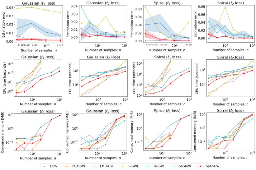
Figure 5: Comparison on estimation error (Top), CPU time (Middle), and consumed memory (Bottom) for approximating GW distances. The mean and standard deviation are reported for sampling-based methods.

Figure 5 shows the estimation error compared to PGA-GW (top row), the CPU time (middle row), and the consumed memory (bottom row) versus increasing $n$. Memory consumption is measured by the difference between peak and initial memory. We observe that our Spar-GW method consistently reaches similar or even better accuracy while being orders of magnitude faster than EGW-based approaches (i.e., EGW, PGA-GW, and EMD-GW), especially for the $\ell_{1}$ loss. We also observe that all these methods require similar memory, and this observation is consistent with the fact that these methods have the same order of memory complexity $O(n^{2})$. These observations demonstrate that the proposed Spar-GW method is exceedingly competitive with classical EGW-based methods, requiring much less computational cost.

C.2 Approximation of fused GW distance

We evaluate the approximation performance of Spar-FGW algorithm w.r.t. FGW distances, on Moon and Graph datasets in Fig. 6. The results of Gaussian and Spiral datasets are similar to those of Moon, and thus have been omitted here.

Figure 6: Comparison on estimation error (Top) and CPU time (Bottom) w.r.t. FGW distance. The mean and standard deviation are reported for sampling-based methods.

In Fig. 6, we add another baseline, i.e., the naive transport plan $\mathbf{T}=\bm{a}\bm{b}^{\top}$. Other competitors are adapted to approximate the FGW distance for comparison. The source and target attributes are generated from multidimensional Gaussian distributions $N(0\times\bm{1}_{5},10\times\mathbf{I}_{5})$ and $N(5\times\bm{1}_{5},10\times\mathbf{I}_{5})$, respectively, and the feature distance matrix $\mathbf{M}$ is defined by their pairwise Euclidean distances in $\mathbb{R}^{5}$. The trade-off parameter $\alpha$ in (10) is set to be 0.6. Results in Fig. 6 show that Spar-FGW yields the most accurate estimation with the best scalability in most cases.

References

• Achlioptas and Mcsherry, (2007) Achlioptas, D. and Mcsherry, F. (2007). Fast computation of low-rank matrix approximations. Journal of the Association for Computing Machinery, 54(2):1–19.
• Alaux et al., (2019) Alaux, J., Grave, E., Cuturi, M., and Joulin, A. (2019). Unsupervised hyper-alignment for multilingual word embeddings. In 7th International Conference on Learning Representations, New Orleans, LA, USA.
• Alvarez-Melis and Jaakkola, (2018) Alvarez-Melis, D. and Jaakkola, T. (2018). Gromov-Wasserstein alignment of word embedding spaces. In Proceedings of the 2018 Conference on Empirical Methods in Natural Language Processing, pages 1881–1890, Brussels, Belgium. ACL.
• Benamou et al., (2002) Benamou, J.-D., Brenier, Y., and Guittet, K. (2002). The Monge–Kantorovitch mass transfer and its computational fluid mechanics formulation. International Journal for Numerical Methods in Fluids, 40(1-2):21–30.
• Blumberg et al., (2020) Blumberg, A. J., Carriere, M., Mandell, M. A., Rabadan, R., and Villar, S. (2020). MREC: a fast and versatile framework for aligning and matching point clouds with applications to single cell molecular data. arXiv preprint arXiv:2001.01666.
• Bonneel et al., (2015) Bonneel, N., Rabin, J., Peyré, G., and Pfister, H. (2015). Sliced and Radon Wasserstein barycenters of measures. Journal of Mathematical Imaging and Vision, 51(1):22–45.
• Bonneel et al., (2011) Bonneel, N., van de Panne, M., Paris, S., and Heidrich, W. (2011). Displacement interpolation using Lagrangian mass transport. ACM Transactions on Graphics, 30(6):1–12.
• Braverman et al., (2021) Braverman, V., Krauthgamer, R., Krishnan, A. R., and Sapir, S. (2021). Near-optimal entrywise sampling of numerically sparse matrices. In Conference on Learning Theory, pages 759–773. PMLR.
• Brenier, (1997) Brenier, Y. (1997). A homogenized model for vortex sheets. Archive for Rational Mechanics and Analysis, 138(4):319–353.
• Brogat-Motte et al., (2022) Brogat-Motte, L., Flamary, R., Brouard, C., Rousu, J., and d’Alché Buc, F. (2022). Learning to predict graphs with fused Gromov-Wasserstein barycenters. In International Conference on Machine Learning, pages 2321–2335. PMLR.
• Bunne et al., (2019) Bunne, C., Alvarez-Melis, D., Krause, A., and Jegelka, S. (2019). Learning generative models across incomparable spaces. In International Conference on Machine Learning, pages 851–861. PMLR.
• Chapel et al., (2020) Chapel, L., Alaya, M. Z., and Gasso, G. (2020). Partial optimal tranport with applications on positive-unlabeled learning. Advances in Neural Information Processing Systems, 33:2903–2913.
• (13) Chizat, L., Peyré, G., Schmitzer, B., and Vialard, F.-X. (2018a). An interpolating distance between optimal transport and Fisher-Rao metrics. Foundations of Computational Mathematics, 18(1):1–44.
• (14) Chizat, L., Peyré, G., Schmitzer, B., and Vialard, F.-X. (2018b). Scaling algorithms for unbalanced optimal transport problems. Mathematics of Computation, 87(314):2563–2609.
• (15) Chizat, L., Peyré, G., Schmitzer, B., and Vialard, F.-X. (2018c). Unbalanced optimal transport: Dynamic and Kantorovich formulations. Journal of Functional Analysis, 274(11):3090–3123.
• Chowdhury and Mémoli, (2019) Chowdhury, S. and Mémoli, F. (2019). The Gromov-Wasserstein distance between networks and stable network invariants. Information and Inference: A Journal of the IMA, 8(4):757–787.
• Chowdhury et al., (2021) Chowdhury, S., Miller, D., and Needham, T. (2021). Quantized Gromov-Wasserstein. In Joint European Conference on Machine Learning and Knowledge Discovery in Databases, pages 811–827. Springer.
• Chowdhury and Needham, (2021) Chowdhury, S. and Needham, T. (2021). Generalized spectral clustering via Gromov-Wasserstein learning. In Proceedings of the 24th International Conference on Artificial Intelligence and Statistics, volume 130, pages 712–720. PMLR.
• Cuturi, (2013) Cuturi, M. (2013). Sinkhorn distances: Lightspeed computation of optimal transport. Advances in Neural Information Processing Systems, 26:2292–2300.
• Deshpande et al., (2019) Deshpande, I., Hu, Y.-T., Sun, R., Pyrros, A., Siddiqui, N., Koyejo, S., Zhao, Z., Forsyth, D., and Schwing, A. G. (2019). Max-sliced Wasserstein distance and its use for GANs. In Proceedings of the IEEE/CVF Conference on Computer Vision and Pattern Recognition, pages 10648–10656. IEEE.
• Ezuz et al., (2017) Ezuz, D., Solomon, J., Kim, V. G., and Ben-Chen, M. (2017). GWCNN: A metric alignment layer for deep shape analysis. In Computer Graphics Forum, volume 36, pages 49–57. Wiley Online Library.
• Feragen et al., (2013) Feragen, A., Kasenburg, N., Petersen, J., de Bruijne, M., and Borgwardt, K. (2013). Scalable kernels for graphs with continuous attributes. Advances in Neural Information Processing Systems, 26:216–224.
• Fey and Lenssen, (2019) Fey, M. and Lenssen, J. E. (2019). Fast graph representation learning with PyTorch Geometric. ICLR Workshop on Representation Learning on Graphs and Manifolds.
• Genevay et al., (2019) Genevay, A., Chizat, L., Bach, F., Cuturi, M., and Peyré, G. (2019). Sample complexity of Sinkhorn divergences. In 22nd International Conference on Artificial Intelligence and Statistics, pages 1574–1583. PMLR.
• Gong et al., (2022) Gong, F., Nie, Y., and Xu, H. (2022). Gromov-Wasserstein multi-modal alignment and clustering. In Proceedings of the 31st ACM International Conference on Information & Knowledge Management, pages 603–613.
• Hagberg et al., (2008) Hagberg, A. A., Schult, D. A., and Swart, P. J. (2008). Exploring network structure, dynamics, and function using NetworkX. In Proceedings of the 7th Python in Science Conference, pages 11–15, Pasadena, CA, USA.
• Kantorovich, (1942) Kantorovich, L. (1942). On the transfer of masses (in Russian). In Doklady Akademii Nauk, volume 37, pages 227–229.
• Kawano and Mason, (2021) Kawano, S. and Mason, J. K. (2021). Classification of atomic environments via the Gromov-Wasserstein distance. Computational Materials Science, 188:110144.
• Kerdoncuff et al., (2021) Kerdoncuff, T., Emonet, R., and Sebban, M. (2021). Sampled Gromov Wasserstein. Machine Learning, 110(8):2151–2186.
• Kriege et al., (2018) Kriege, N. M., Fey, M., Fisseler, D., Mutzel, P., and Weichert, F. (2018). Recognizing cuneiform signs using graph based methods. In International Workshop on Cost-Sensitive Learning, pages 31–44. PMLR.
• Le et al., (2021) Le, T., Ho, N., and Yamada, M. (2021). Flow-based alignment approaches for probability measures in different spaces. In International Conference on Artificial Intelligence and Statistics, pages 3934–3942. PMLR.
• Li et al., (2022) Li, T., Meng, C., Yu, J., and Xu, H. (2022). Hilbert curve projection distance for distribution comparison. arXiv preprint arXiv:2205.15059.
• (33) Liao, Q., Chen, J., Wang, Z., Bai, B., Jin, S., and Wu, H. (2022a). Fast Sinkhorn I: An ${O}({N})$ algorithm for the Wasserstein-1 metric. arXiv preprint arXiv:2202.10042.
• (34) Liao, Q., Wang, Z., Chen, J., Bai, B., Jin, S., and Wu, H. (2022b). Fast Sinkhorn II: Collinear triangular matrix and linear time accurate computation of optimal transport. arXiv preprint arXiv:2206.09049.
• Liero et al., (2016) Liero, M., Mielke, A., and Savaré, G. (2016). Optimal transport in competition with reaction: The Hellinger-Kantorovich distance and geodesic curves. SIAM Journal on Mathematical Analysis, 48(4):2869–2911.
• Lin et al., (2019) Lin, T., Ho, N., and Jordan, M. I. (2019). On the acceleration of the Sinkhorn and Greenkhorn algorithms for optimal transport. arXiv preprint arXiv:1906.01437.
• Liu, (1996) Liu, J. S. (1996). Metropolized independent sampling with comparisons to rejection sampling and importance sampling. Statistics and Computing, 6(2):113–119.
• Liu, (2008) Liu, J. S. (2008). Monte Carlo Strategies in Scientific Computing. Springer.
• Luo et al., (2022) Luo, D., Wang, Y., Yue, A., and Xu, H. (2022). Weakly-supervised temporal action alignment driven by unbalanced spectral fused Gromov-Wasserstein distance. In Proceedings of the 30th ACM International Conference on Multimedia, pages 728–739.
• Ma et al., (2015) Ma, P., Mahoney, M. W., and Yu, B. (2015). A statistical perspective on algorithmic leveraging. The Journal of Machine Learning Research, 16(1):861–911.
• Mémoli, (2011) Mémoli, F. (2011). Gromov-Wasserstein distances and the metric approach to object matching. Foundations of Computational Mathematics, 11(4):417–487.
• Meng et al., (2019) Meng, C., Ke, Y., Zhang, J., Zhang, M., Zhong, W., and Ma, P. (2019). Large-scale optimal transport map estimation using projection pursuit. Advances in Neural Information Processing Systems, 32:8118–8129.
• Muzellec et al., (2020) Muzellec, B., Josse, J., Boyer, C., and Cuturi, M. (2020). Missing data imputation using optimal transport. In International Conference on Machine Learning, pages 7130–7140. PMLR.
• Nadjahi, (2021) Nadjahi, K. (2021). Sliced-Wasserstein Distance for Large-Scale Machine Learning: Theory, Methodology and Extensions. PhD thesis, Institut polytechnique de Paris.
• Neumann et al., (2013) Neumann, M., Moreno, P., Antanas, L., Garnett, R., and Kersting, K. (2013). Graph kernels for object category prediction in task-dependent robot grasping. In Online Proceedings of the Eleventh Workshop on Mining and Learning with Graphs, pages 10–6, Chicago, Illinois, USA. ACM.
• Pedregosa et al., (2011) Pedregosa, F., Varoquaux, G., Gramfort, A., Michel, V., Thirion, B., Grisel, O., Blondel, M., Prettenhofer, P., Weiss, R., Dubourg, V., et al. (2011). Scikit-learn: Machine learning in Python. The Journal of Machine Learning Research, 12:2825–2830.
• Peyré and Cuturi, (2019) Peyré, G. and Cuturi, M. (2019). Computational optimal transport: With applications to data science. Foundations and Trends® in Machine Learning, 11(5-6):355–607.
• Peyré et al., (2016) Peyré, G., Cuturi, M., and Solomon, J. (2016). Gromov-Wasserstein averaging of kernel and distance matrices. In International Conference on Machine Learning, pages 2664–2672. PMLR.
• Pham et al., (2020) Pham, K., Le, K., Ho, N., Pham, T., and Bui, H. (2020). On unbalanced optimal transport: An analysis of Sinkhorn algorithm. In International Conference on Machine Learning, pages 7673–7682. PMLR.
• Rand, (1971) Rand, W. M. (1971). Objective criteria for the evaluation of clustering methods. Journal of the American Statistical Association, 66(336):846–850.
• Reddi et al., (2016) Reddi, S. J., Sra, S., Póczos, B., and Smola, A. (2016). Stochastic Frank-Wolfe methods for nonconvex optimization. In 2016 54th Annual Allerton Conference on Communication, Control, and Computing (Allerton), pages 1244–1251. IEEE.
• Sato et al., (2020) Sato, R., Cuturi, M., Yamada, M., and Kashima, H. (2020). Fast and robust comparison of probability measures in heterogeneous spaces. arXiv preprint arXiv:2002.01615.
• Scetbon and Cuturi, (2020) Scetbon, M. and Cuturi, M. (2020). Linear time Sinkhorn divergences using positive features. Advances in Neural Information Processing Systems, 33:13468–13480.
• Scetbon et al., (2022) Scetbon, M., Peyré, G., and Cuturi, M. (2022). Linear-time Gromov Wasserstein distances using low rank couplings and costs. In International Conference on Machine Learning, pages 19347–19365. PMLR.
• Séjourné et al., (2021) Séjourné, T., Vialard, F.-X., and Peyré, G. (2021). The unbalanced Gromov Wasserstein distance: Conic formulation and relaxation. Advances in Neural Information Processing Systems, 34:8766–8779.
• Sinkhorn and Knopp, (1967) Sinkhorn, R. and Knopp, P. (1967). Concerning nonnegative matrices and doubly stochastic matrices. Pacific Journal of Mathematics, 21(2):343–348.
• Solomon et al., (2016) Solomon, J., Peyré, G., Kim, V. G., and Sra, S. (2016). Entropic metric alignment for correspondence problems. ACM Transactions on Graphics, 35(4):1–13.
• Sturm, (2006) Sturm, K.-T. (2006). On the geometry of metric measure spaces. Acta Mathematica, 196(1):65–131.
• Sutherland et al., (2003) Sutherland, J. J., O’brien, L. A., and Weaver, D. F. (2003). Spline-fitting with a genetic algorithm: A method for developing classification structure-activity relationships. Journal of Chemical Information and Computer Sciences, 43(6):1906–1915.
• (60) Titouan, V., Courty, N., Tavenard, R., and Flamary, R. (2019a). Optimal transport for structured data with application on graphs. In International Conference on Machine Learning, pages 6275–6284. PMLR.
• (61) Titouan, V., Flamary, R., Courty, N., Tavenard, R., and Chapel, L. (2019b). Sliced Gromov-Wasserstein. Advances in Neural Information Processing Systems, 32:14753–14763.
• Vayer et al., (2020) Vayer, T., Chapel, L., Flamary, R., Tavenard, R., and Courty, N. (2020). Fused Gromov-Wasserstein distance for structured objects. Algorithms, 13(9):212.
• Villani, (2009) Villani, C. (2009). Optimal Transport: Old and New, volume 338. Springer.
• Vincent-Cuaz et al., (2022) Vincent-Cuaz, C., Flamary, R., Corneli, M., Vayer, T., and Courty, N. (2022). Semi-relaxed Gromov-Wasserstein divergence with applications on graphs. In 10th International Conference on Learning Representations.
• Weitkamp et al., (2020) Weitkamp, C. A., Proksch, K., Tameling, C., and Munk, A. (2020). Gromov-Wasserstein distance based object matching: asymptotic inference. arXiv preprint arXiv:2006.12287.
• Xie et al., (2020) Xie, Y., Wang, X., Wang, R., and Zha, H. (2020). A fast proximal point method for computing exact Wasserstein distance. In Uncertainty in Artificial Intelligence, pages 433–453. PMLR.
• Xu et al., (2023) Xu, H., Liu, J., Luo, D., and Carin, L. (2023). Representing graphs via Gromov-Wasserstein factorization. IEEE Transactions on Pattern Analysis and Machine Intelligence, 45(1):999–1016.
• (68) Xu, H., Luo, D., and Carin, L. (2019a). Scalable Gromov-Wasserstein learning for graph partitioning and matching. Advances in Neural Information Processing Systems, 32:3052–3062.
• (69) Xu, H., Luo, D., Zha, H., and Carin, L. (2019b). Gromov-Wasserstein learning for graph matching and node embedding. In International Conference on Machine Learning, pages 6932–6941. PMLR.
• Yan et al., (2018) Yan, Y., Li, W., Wu, H., Min, H., Tan, M., and Wu, Q. (2018). Semi-supervised optimal transport for heterogeneous domain adaptation. In Proceedings of the 27th International Joint Conference on Artificial Intelligence, pages 2969–2975.
• Yanardag and Vishwanathan, (2015) Yanardag, P. and Vishwanathan, S. (2015). Deep graph kernels. In Proceedings of the 21th ACM SIGKDD International Conference on Knowledge Discovery and Data Mining, pages 1365–1374.
• Yu et al., (2022) Yu, J., Wang, H., Ai, M., and Zhang, H. (2022). Optimal distributed subsampling for maximum quasi-likelihood estimators with massive data. Journal of the American Statistical Association, 117(537):265–276.
• Zhang et al., (2022) Zhang, J., Ma, P., Zhong, W., and Meng, C. (2022). Projection-based techniques for high-dimensional optimal transport problems. Wiley Interdisciplinary Reviews: Computational Statistics, page e1587.