Anatomy of single-field inflationary models for primordial black holes

Abstract

We construct an analytically solvable simplified model that captures the essential features for primordial black hole (PBH) production in most models of single-field inflation. The construction makes use of the Wands duality between the constant-roll (or slow-roll) and the preceding ultra-slow-roll phases and can be realized by a simple inflaton potential of two joined parabolas. Within this framework, it is possible to formulate explicit inflationary scenarios consistent with the CMB observations and copious production of PBHs of arbitrary mass. We quantify the variability of the shape of the peak in the curvature power spectrum in different inflationary scenarios and discuss its implications for probing PBHs with scalar-induced gravitational wave backgrounds. We find that the COBE/Firas $\mu$-distortion constraints exclude the production of PBHs heavier than $10^{4}M_{\odot}$ in single-field inflation.

1 Introduction

The existence of dark matter (DM) has been clearly established via its gravitational effect on cosmic structures, yet its nature and origin has eluded us for almost a century [1]. The LIGO-Virgo collaboration’s discovery of gravitational waves (GWs) [2, 3, 4, 5] originating from binary black hole (BH) mergers together with the absence of observational signatures of particle DM has reinvigorated interest on primordial black holes (PBHs) [6, 7] as a potential DM candidate [8, 9, 10]. However, numerous experiments have placed bounds on the PBH abundance (see e.g. [11] for a recent review) and PBHs are allowed to make up the entirety of DM only in the asteroid mass window $10^{17}\,{\rm g}\lesssim M_{\rm PBH}\lesssim 10^{21}\,{\rm g}$ [12, 13, 14]. Nevertheless, PBHs in the solar mass range could still contribute to the LIGO-Virgo merger events if solar mass PBHs make up about 0.1% of the DM energy budget [15, 16, 17, 18, 19, 20, 21, 22, 23, 24, 25, 26]. PBHs heavier than $10^{3}M_{\odot}$ can provide seeds for supermassive BHs [27, 28, 29] and play a role in generating cosmic structures [29].

PBHs can form via various channels in the early Universe (see e.g. [30, 11] for reviews). The most commonly considered scenario involves the collapse of large density perturbations generated during inflation [31, 32, 33, 34, 35, 36, 37, 38, 39, 40, 41, 42, 43, 44, 45, 46, 47, 48, 49, 50, 51, 52, 53, 54, 55, 56, 57, 58, 59, 60, 61, 62, 63, 64, 65, 66, 67, 68, 69, 70, 71, 72, 73, 74, 75, 76, 77, 78, 79, 80, 81, 82, 83, 84, 85, 86, 87, 88, 89, 90, 91, 92, 93, 94, 95, 96, 97, 98, 99, 100, 101, 102, 103, 104, 105, 106, 107, 108, 109, 110, 111, 112], but they may be produced also in cosmological phase transitions [113, 114, 115], by the collapse of cosmic strings [116, 117, 118, 119, 120, 121, 122], false vacuum bubbles [123, 124, 125, 126, 127, 128] or domain walls [129, 130, 131, 132, 133], or post-inflationary scalar field fragmentation [134, 135, 136]. These PBH formation scenarios could be probed indirectly via the associated GW background. In particular, large scalar perturbations during inflation induce a stochastic GW background via mode coupling at the second perturbative order [137, 138, 139, 140, 141] (for a recent review, see [142]). This GW background has not been seen so far by LIGO-Virgo [143, 144], but it has been suggested that the recent signal from pulsar timing experiments at nHz frequencies [145, 146, 147, 148] could be related to GWs accompanying PBH formation from large inflationary scalar perturbations [149, 150, 151, 152].

In this paper, we will focus on single-field inflationary scenarios for PBHs, which typically require potentials with specific features capable of inducing peaks in the curvature power spectrum. Over the past three decades, a large number of such models have been proposed [39, 40, 41, 42, 43, 44, 45, 46, 47, 48, 49, 50, 51, 52, 53, 54, 55, 56, 57, 58, 59, 60, 61, 62, 63, 64, 65, 66, 67, 68, 69, 70, 71, 72, 73, 74, 75, 76, 77, 78, 79, 80, 81, 82, 83, 84, 85, 86, 87, 88, 89, 90, 91, 92, 93, 94, 95, 96, 97, 98, 99, 100, 101, 102, 103, 104, 105, 106, 107, 108, 109, 110, 111, 112]. We will briefly review them in the following.

The first toy model was developed in 1994 by Ivanov et al. [39], where they considered a potential with two power-law regions separated by a plateau. Similarly, an early toy model assumed a cliff-like feature where the slope becomes abruptly steeper [41]. Although these models can produce large spikes in the power spectrum, they also predict a blue tilt at the CMB scales, which is now excluded.

The first theoretically-motivated model was proposed in the context of supergravity [42] (and was further developed in [43, 50]). In this scenario, a specific choice for the superpotential generates a polynomial inflaton potential, which, together with a complicated “pre-inflation” phase, produces a power spectrum with a high amplitude and a shallow slope ($n_{s}<1$) on small scales and a low amplitude and a nearly scale-invariant spectrum ($n_{s}\sim 1$) on large scales.

Inflation from a Coleman-Weinberg type potential $V\propto\phi^{4}\ln(\phi^{2}/\mu^{2})$ could produce two inflationary phases [44, 46, 47]—chaotic inflation followed by crossing the minimum and a near-stop close to the origin which causes a second phase of inflation. A similar scenario is possible with the double well potential [47] (see also [84]). Unfortunately, the Coleman-Weinberg potential predicts a very large tensor-to-scalar ratio ($r>0.3$) and a quite small scalar spectral index ($n_{s}<0.94$).

In the running mass model [45, 48, 49] (see also [56]), $V(\phi)=V_{0}\pm m^{2}(\phi)\phi^{2}/2$, obtained from softly broken global supersymmetry, the power spectrum does not feature a peak, but instead it grows continuously on small scales. This feature can produce an overabundance of PBHs and, furthermore, result in eternal inflation unless a “waterfall” field is introduced to force inflation to end.

More recently, a simple, theoretically well-motivated scenario involving a non-minimally coupled inflaton with a general quartic potential has been considered [54, 58, 59]. In this scenario, the Einstein frame possesses a quasi-inflection point (a small local maximum) for PBH production, and the non-minimal coupling leads to a plateau at large field values guaranteeing a small tensor-to-scalar ratio. However, non-minimal polynomial inflation with at most quartic terms will generally give a small scalar spectral index ($n_{s}<0.95$) when it produces PBHs with lifetimes exceeding the age of the Universe [54, 58, 59]. This issue can be solved by quantum corrections, such as threshold effects in running couplings [54] or effective higher-order operators [59]. A very similar scenario was initially considered in Ref. [51] (see also [57, 60, 74, 75, 89]), in which the Einstein frame potential of non-minimal quartic inflation was used, but without the field redefinition that arises when moving from the Jordan frame to the Einstein frame.

In the context of quasi-inflection point scenarios, it was shown that, around the small maximum, the slow-roll (SR) conditions fail, and the inflaton enters a temporary ultra-slow-roll (USR) phase during which it will slow down considerably [54, 55, 56]. During this process, a sizeable peak in the spectrum can be generated. As a result, the usual SR approximation for the curvature power spectrum breaks down, and the Mukhanov-Sasaki equation must be solved numerically to obtain accurate results. In most cases, the potential parameters must be tuned to the precision of several significant digits as the field has to be balanced on top of a small local maximum for tens of $e$-folds before rolling over it.

Once it became widely understood that an asymptotically flat potential that features a quasi-inflection point at smaller field values can potentially produce PBHs and drive otherwise observationally successful inflation, a plethora of new models were suggested. Perhaps the most physically-motivated and economic of them is Critical Higgs Inflation [53] (see also [58, 73]). In this model, the non-minimally coupled Standard Model Higgs field is taken to be the inflaton. It has a simple quartic potential which gets logarithmic corrections once one considers the RG running of the quartic and non-minimal couplings. However, in [67], the model was studied carefully in both metric and Palatini formalisms and it was shown that one could obtain inflationary predictions in agreement with the experimental constraints only if $M_{\rm PBH}<10^{6}\ \rm g$.

Inflaton potentials with a quasi-inflection point can also arise in models of string inflation [61, 62, 111], string-inspired axion monodromy [81], superconformal attractors [65, 71] (see also [87, 108]), and no-scale supergravity [66, 85, 92, 93]. Most of these models comply with the inflationary constraints and predict PBH DM in the asteroid mass window, $M_{\rm PBH}\sim 10^{-16}\ M_{\odot}-10^{-13}\ M_{\odot}$.

Large peaks in the power spectrum can also be induced by introducing a dump/dip or a step to the potential. In the bumpy/dippy models [72, 77, 80, 97, 103, 107], a small, often a Gaussian bump/dip multiplies a base potential. As bumps and dips can be placed anywhere in the potential, they can produce PBHs in a wide range of masses. Interestingly, a base potential with $n_{s}\geq 0.98$, excluded by CMB observations [153], becomes favoured when modified by the bump/dip. This is because the inflaton typically spends an extra $10-15$ $e$-folds during the power spectrum amplification near the bump/dip, reducing the length of the remaining SR period to at most 45-50 $e$-folds and thus results in a decrease in the value of $n_{s}$ as it is determined only by the latter. Similarly, one (or multiple) steep step(s) in the potential can lead to a strongly enhanced oscillating power spectrum [88, 91, 95, 104, 110].

All models discussed above contain a feature in the potential. An alternative is to keep the potential simple and featureless but modify the gravitational component of the action beyond a simple non-minimal coupling. Examples of these models include $F(R)$ gravity [112], Dirac-Born-Infeld inflation [68], a non-minimal derivative coupling between the inflaton and gravity [76, 83, 100, 105], Gauss-Bonnet inflation [101], warm inflation [78, 94], axion inflation with gauge fields [86], $G$- or $k$-inflation [90, 96, 99]. Typically, in these models, the enhancement of the power spectrum arises due to its modified expression, which, apart from the potential, also depends on the extra non-minimal functions of the scalar field.

To sum up, inflationary models used for PBH production can be classified into two general categories:

1. Models where the (Einstein frame) inflationary potential contains a feature. These, in turn, can be subdivided into three categories:

   • Small local maximum (which includes upward steps and quasi-inflection points) [54, 58, 59, 51, 57, 60, 74, 75, 89, 55, 56, 53, 73, 67, 61, 62, 111, 81, 65, 71, 87, 108, 66, 85, 92, 93, 72, 77, 80, 97, 103, 107, 110]

   • Downward steps [88, 91, 95, 104]

   • Rolling through the global minimum [44, 46, 47, 84]

   • Potentials with multiple features stacked on top of each other, for instance, rapid oscillations [154] (see also [155]).

2. Modified gravity (beyond non-minimally coupled inflaton) with features in terms other than the inflaton potential or the non-minimal coupling [112, 68, 76, 83, 100, 105, 101, 78, 82, 94, 86, 90, 96, 99].

The general behaviour of the power spectrum during the rapid transition from SR inflation to non-attractor inflation is of great importance for the resulting PBH phenomenology. Consequently, it is desirable to have analytic models for said behaviour. This is possible if one considers toy models in which the evolution of SR parameters is postulated instead of derived from solving the field equations. For example, in [156] it was shown that in single-field inflation, independently of the shape of the inflaton potential, the steepest possible growth of the primordial power spectrum is $n_{s}-1=4$, or equivalently, $k^{4}$, with $k$ being the comoving scale. A further refined analysis [157], however, showed that a steeper $k^{5}\left(\log k\right)^{2}$ growth can be possible (see also [154, 158, 159, 160, 87, 155, 89, 161]). However, growth steeper than $k^{4}$ will not have any measurable impact on the PBH mass function [162] and, as we will show, requires an initial phase of inflation with a blue-tilted spectrum.

In this paper, we consider the general class of single-field inflation models in which an Einstein frame can be defined. We outline the essential qualitative features of these scenarios and propose a novel, analytically solvable model capable of capturing these features. Our analytic method uses the Wands duality [163] between the USR and the subsequent constant-roll (CR) (or SR) phase, which is present in most single-field models for PBHs. Thus, it improves upon existing analytic approaches built around specific ansätze for the second SR parameter [156, 157, 162]. Moreover, we show that our analytic model corresponds to a continuous potential constructed by gluing together two parabolas and can thus be seen as a limiting case of realistic inflationary scenarios. It can also be thought of as a generalization of the Starobinsky model [164], in which the potential consists of two linear segments with different slopes. Although we will not consider models with multiple features, the proposed analytic approach can be straightforwardly generalized to include such scenarios.

Having approximate analytic tools at hand is beneficial not only for theoretical studies but also for inflationary model building and PBH phenomenology. Using various shapes for the power spectra, we analyse the potential of future GW experiments for probing the GW background induced by the large scalar perturbations in single-field inflation, showing that the windows where the PBHs could constitute all DM and where they could contribute to the LIGO-Virgo GW events, can be probed with the future GW interferometers and pulsar timing arrays, respectively [165, 166, 167, 168, 169, 170, 171, 172, 156, 173, 174, 175, 176, 177, 178]. These analytical tools can also be applied to improve limits on heavy PBH scenarios, e.g., by using COBE/Firas $\mu$-distortion constraints [179, 180, 181].

The paper is structured as follows: Section 2 outlines the general mathematical framework of inflation, cosmological perturbations and the general phases of single-field inflationary models for PBHs. In section 3, we introduce the instantaneous SR to USR approximation, derive the corresponding analytic curvature power spectrum, and construct the corresponding inflationary potential. Non-instantaneous SR to USR transitions and the application of our analytic approximations to the study of spectra for general potentials are discussed in section 4. Section 5 deals with the resulting PBH and GW phenomenology. We conclude in section 6. We use natural units $c=\hbar=1$.

2 General considerations

Inflationary PBH production within single-field inflation typically requires for inflation to proceed in two or more phases of SR or constant-roll (CR), separated by a brief exit from SR and a transient USR phase. The latter is responsible for the super-horizon enhancement of the scalar modes that exited the cosmological horizon around this transient phase [182, 183] and will ultimately determine the position and height of the peak in the power spectrum responsible for PBH creation. The slope of the enhanced peak at the end of the USR phase generally mimics the spectrum created in the subsequent CR phase due to the Wands duality [163]. This makes it possible to infer the qualitative features of the power spectrum, e.g., the height and the position of the generated peak, from background evolution alone, similarly to SR inflation. However, an accurate estimate of the shape of the peak requires a numerical approach to the evolution of individual modes, i.e., via applying the Mukhanov-Sasaki (MS) equation.

2.1 Background evolution in single-field inflation

In the Einstein frame, single-field inflation is described by the following action:

$$\mathcal{S}=\int{{\rm d}x^{4}\sqrt{-g}\left(\frac{M_{\rm P}^{2}}{2}R-\frac{1}{2}\partial^{\mu}\phi\partial_{\mu}\phi-V(\phi)\right)}\,,$$ (2.1)

where $R$ is the Ricci scalar, $V(\phi)$ is the inflaton potential and $M_{\rm P}$ the reduced Planck mass. We consider a flat FLRW background geometry ${\rm d}s^{2}=-{\rm d}t^{2}+a^{2}{\rm d}x_{i}^{2}$, where $a$ is the scale factor. The evolution of the scale factor and the inflaton are governed by the Friedmann equation $3M_{\rm P}^{2}H^{2}=\dot{\phi}^{2}/2+V(\phi)$, and the Klein-Gordon equation $\ddot{\phi}+3H\dot{\phi}+V^{\prime}=0$, respectively. The overdot indicates differentiation with respect to the cosmic time $t$, a prime denotes differentiation with respect to the scalar field $\phi$ and $H\equiv\dot{a}/a$ is the Hubble parameter. This approach includes all models in which the Einstein frame exists, e.g., non-minimally coupled inflatons or non-canonical inflaton kinetic terms. Theories with higher-order Einstein frame kinetic terms, such as $(\partial\phi)^{4}$, may be approximated by this class, if these higher-order terms are subdominant even when SR is violated, e.g., as in Palatini $R^{2}$ gravity [184, 185, 186, 187]. Permitting disformal transformations [188, 189, 190, 191], this also includes some Horndeski theories [192, 193].

In the following, we will measure time in $e$-folds, $N\equiv\ln a$. The field equations can be then be recast as

$$\partial_{N}y+\left(3-\frac{y^{2}}{2}\right)\left(y+M_{\rm P}\frac{V^{\prime}}{V}\right)=0,\qquad y\equiv\frac{\partial_{N}\phi}{M_{\rm P}}\,,$$ (2.2)

and the Hubble parameter can be expressed as a function of $\phi$ and $y$ via $M_{\rm P}^{2}H^{2}=V(\phi)(3-y^{2}/2)^{-1}$. The SR approximation is obtained by ignoring the $\partial_{N}y$ term in Eq. (2.2) and the field equations are given by setting the last bracket in (2.2) to zero, i.e., $y+M_{\rm P}\partial_{\phi}\ln V=0$. SR and deviations from it are conveniently described in terms of the Hubble SR parameters

$$\epsilon_{H}\equiv\frac{1}{2}y^{2}=-\frac{\dot{H}}{H^{2}}\,,\qquad\eta_{H}=-\partial_{N}\ln y+\epsilon_{H}=-\frac{\ddot{H}}{2H\dot{H}}\,.$$ (2.3)

Inflation occurs as long as $\epsilon_{H}<1$, while the SR approximation holds as long as both SR parameters are small ($\epsilon_{H},\eta_{H}\ll 1$). For future reference we will also define the potential SR parameters

$$\epsilon_{V}\equiv\frac{M_{\rm P}^{2}}{2}\left(\frac{V^{\prime}}{V}\right)^{2}\,,\qquad\eta_{\rm V}\equiv M_{\rm P}^{2}\,\frac{V^{\prime\prime}}{V}\,\,,$$ (2.4)

which satisfy $\epsilon_{V}\approx\epsilon_{H}\,,\eta_{V}\approx\eta_{H}+\epsilon_{H}\,$ at the leading order in SR.

2.2 Evolution of the curvature perturbations

The evolution of the scalar curvature perturbation $\mathcal{R}_{c}$ is conveniently studied using the so-called Mukhanov field $u\equiv z\mathcal{R}_{c}$, where

$$z\equiv a\dot{\phi}/H=ayM_{\rm P}\,.$$ (2.5)

The Fourier modes of $u$ evolve according to the MS equation [194, 195, 196],

$$u_{k}^{\prime\prime}+\left(k^{2}-\frac{z^{\prime\prime}}{z}\right)u_{k}=0\,,$$ (2.6)

where the prime denotes differentiation with respect to conformal time, ${\rm d}\tau={\rm d}t/a$. The second term in the parenthesis of the MS equation (2.6) is recast in terms of the SR parameters as

$$\frac{z^{\prime\prime}}{z} =\mathcal{H}^{2}\left[2-\left(3-\epsilon_{H}\right)\eta_{V}+\epsilon_{H}\left(5+2\epsilon_{H}-4\eta_{H}\right)\right]\,,$$ (2.7)

where $\mathcal{H}\equiv a^{\prime}/a=aH$. We stress that this expression is exact to all orders in the SR parameters. In the SR phase, the SR parameters are small, implying $z^{\prime\prime}/z\approx 2\mathcal{H}^{2}$. The limits $k^{2}\gg z^{\prime\prime}/z$ and $k^{2}\ll z^{\prime\prime}/z$ correspond to the sub-horizon and super-horizon evolution of the mode, respectively. Both $z$ and $z^{\prime\prime}/z$ are monotonously growing functions during SR, so these limits occur at $N\to-\infty$ and $N\to+\infty$, respectively. However, if the inflationary universe contains a SR-violating phase such as USR, which is generally needed for producing a non-negligible PBH abundance, then $z$ may temporarily decrease, affecting the modes that exit the horizon around that time. Nevertheless, both $z$ and $z^{\prime\prime}/z$ will still be monotonously growing functions of time in the asymptotic past and future.

In the sub-horizon regime, when $k^{2}\gg z^{\prime\prime}/z$, the effect of the curvature of spacetime is negligible and thus the mode $u_{k}$ behaves as a free field on flat spacetime. In the Bunch-Davies vacuum, the normalized solution asymptotes to

$$u_{k}=\frac{1}{\sqrt{2k}}e^{-ik\tau}\,$$ (2.8)

in the limit $\tau\to-\infty$. This serves as the initial condition for the MS equation.

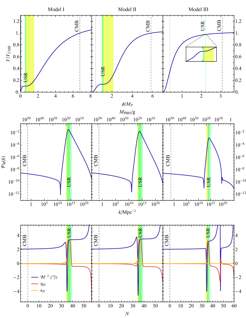
Figure 1: Examples of three inflationary models from the literature producing PBHs in the asteroid mass window [54, 58, 59, 65, 80]. The models and their parameters are detailed in appendix A. The vertical bands correspond to different non-SR epochs: the USR epoch (green), the transition from SR to USR (yellow) and the transition out of USR to the subsequent CR phase (light green). For the power spectrum, they highlight the modes that exited during the corresponding epoch. The dashed vertical line corresponds to the CMB scale. The dotted vertical line in the top panel corresponds to the end of inflation; in the other panels, the end of inflation coincides with the right edge of the plot. In the bottom panel, $N$ denotes the number of e-folds of expansion starting from the CMB scale. All three potentials exhibit a local maximum around the USR scales.

In the super-horizon regime, that is when $k^{2}\ll z^{\prime\prime}/z$, the general solution $u_{k}=A_{1,k}u^{(1)}_{0}+A_{2,k}u^{(2)}_{0}$ comprises a mode that grows during SR, here $u_{0}^{(1)}$, and a decaying mode $u_{0}^{(2)}$, given by

$$u^{(1)}_{0}\propto z,\qquad u^{(2)}_{0}\propto z\int^{0}_{\tau}\frac{{\rm d}\tau^{\prime}}{z(\tau^{\prime})^{2}}.$$ (2.9)

The former will eventually dominate. Consequently, the amplitude of the curvature perturbations is frozen, that is, $|\mathcal{R}_{c\,k}|=\left\lvert u_{k}/z\right\rvert={\rm const}$. As alluded to above, if SR is momentarily violated in such a way that $z$ starts to decrease, then the growing and decreasing $u_{k}$ modes can be mixed. Therefore, the second mode may come to dominate temporarily, potentially leading to super-horizon evolution of $\mathcal{R}_{c}$; however, eventually $z$ starts to grow again and $\mathcal{R}_{c}$ freezes. This makes it possible to relate the observable perturbations at horizon re-entry with the perturbations produced during inflation while being ignorant about the details of the reheating phase.

The primordial power spectrum is evaluated after horizon crossing

$$\mathcal{P}_{\mathcal{R}}=\left.\frac{k^{3}}{2\pi^{2}}\frac{|u_{k}|^{2}}{z^{2}}\right|_{\mathcal{H}\gg k}\stackrel{{\scriptstyle\rm SR}}{{\approx}}\left.\frac{H^{2}}{8\pi^{2}M_{\rm P}^{2}\epsilon_{H}}\right|_{k=\mathcal{H}}\,,$$ (2.10)

where the second expressions shows the result at leading order in the SR approximation, in which case $|u_{k}|^{2}\to(\mathcal{H}/k)^{2}/(2k)$ and $y$ are evaluated at horizon crossing, i.e., when $k=\mathcal{H}$. During SR, the Hubble SR parameters (2.3) can be replaced by the potential ones (2.4), and the scalar spectral index $n_{s}$ and the tensor-to-scalar ratio $r$ are given by the well known expressions

$$n_{s}\approx 1+2\eta_{V}-6\epsilon_{V}\,,\qquad r\approx 16\epsilon_{V}\,,$$ (2.11)

at the leading order in SR. The curvature power spectrum is relatively unconstrained, except at scales relevant for the CMB. The latest observational constraints [153, 197] imply

$$A_{s} =(2.10\pm 0.03)\times 10^{-9},\quad n_{s}=0.9649\pm 0.0042,\quad r<0.036\qquad$$ (2.12)

at the scale $k_{\rm pivot}=0.05\ {\rm Mpc}^{-1}$ and at $68\%$ CL for $A_{s}$ and $n_{s}$ and $95\%$ for $r$. When running of $n_{s}$ is permitted, the constraints are slightly relaxed to $n_{s}=0.9625\pm 0.0048$. Throughout this paper, we will fix $A_{s}\equiv\mathcal{P}_{\mathcal{R}}(k_{\rm pivot})=2.1\times 10^{-9}$, when the power spectrum predictions involve the CMB scales.

2.3 Phases of single-field inflation for PBHs

In the models under consideration, we identify the following phases of inflation:

SR

We will consider models in which inflation begins with a SR phase. At almost all times during this phase, the SR parameters remain small $\epsilon_{H},|\eta_{H}|\ll 1$ and $\eta_{H}$ slightly negative. For definiteness, we define the initial SR phase via the conditions

$$|\epsilon_{H}|,\,|\eta_{H}|,\,|\epsilon_{3}|<1\,,$$ (2.13)

where $\epsilon_{3}\equiv\partial_{N}\ln(\epsilon_{H}-\eta_{H})$ denotes the third SR parameter, which takes large values in particular when $\eta_{H}$ changes rapidly. With these conventions, we find that the initial SR phase typically ends by violating the $|\epsilon_{3}|<1$ condition in PBH models.

Note the enhancement of modes that exit at the end of the SR phase in Fig. 1. This is due to super-horizon effects induced during the subsequent phases [183], that is, the breakdown of the SR approximation for the power spectrum (2.10) begins already during the SR phase.

T1

The next phase is the transition from SR to USR, which we label as T1. This phase is initiated by a feature in the potential that triggers the exit from SR, that is, its onset is signalled by the violation of any of the SR conditions (2.13). Typically, it is characterized by

$$|\epsilon_{3}|>1\,,$$ (2.14)

so that at the beginning of this phase, $\epsilon_{3}=-1$ and $\eta_{H}$ starts to increase rapidly. When $\epsilon_{H}-\eta_{H}=0$, $\epsilon_{3}$ diverges and changes sign. The phase ends when $\epsilon_{3}$ decreases to $1$. During this period, $\mathcal{H}^{-2}z^{\prime\prime}/z<0$ has a sharp dip, as can be observed in Fig. 1 in which the T1 phase is indicated by yellow bands. As can be seen in the upper panels of Fig. 1, the field excursions during this transition tend to be larger than in the following phases. However, as the field is rapidly moving, it’s generally much shorter than any other phase.

The variations in model building tend to affect this phase the most. On top of the models considered in Fig. 1, all of which contain a small local maximum in the potential, this phase can entail rolling through the global minimum [44, 46, 47] or falling down from steep steps in the potential [88, 91, 95, 104, 110]. Inflation may end ($\epsilon_{H}>1$) briefly during this phase (however, it does not in models shown in Fig. 1).

USR

The USR period starts when the field begins to slow down at a plateau or a hillside in the potential (see examples in Fig. 1). Since $V^{\prime}\lesssim 0$ and $\epsilon_{H}\ll 1$, Eq. (2.2) implies that $\partial_{N}y+3y\lesssim 0$ and thus $\eta_{H}\gtrsim 3$ (see discussion below). Throughout this phase, $\eta_{H}$ is approximately constant, and $\epsilon_{H}\propto a^{-2\eta_{H}}$ decreases rapidly. The USR phase, depicted by a green band in Fig. 1, is quite brief, typically lasting for a few $e$-folds. The peak of the spectrum consists typically of modes that exited during this phase.

T2

The dual USR to CR transition, which we label as T2, is characterized by a sharp decline of $\eta_{H}$. Like T1, we define it via the condition $|\epsilon_{3}|>1$. However, unlike in T1, now also always $\epsilon_{H}\ll 1$. In Fig. 1, this phase is denoted by a light green band. One can observe that $\mathcal{H}^{-2}z^{\prime\prime}/z$ remains constant throughout this phase—because the background evolution enters the MS equation (2.6) only through this quantity, the evolution of the $u_{k}$ modes is unaffected by this transition, and no discernible features are generated in the spectrum during this period.

CR

The final CR period begins when $|\epsilon_{3}|<1$. It is characterized by an almost constant and negative second SR parameter, $\eta_{H}<0$. Note that if $|\eta_{H}|\ll 1$, this can be considered a second period of SR inflation. Nevertheless, we will use the label CR throughout the article. Note that $\mathcal{H}^{-2}z^{\prime\prime}/z$ stays constant throughout the USR, T2 and CR phases, indicating that the CR phase is dual to the USR phase. Since the curvature power spectrum during this phase can be estimated analytically, one can use the duality to infer parts of the spectrum in the two earlier phases. In models considered in the literature (e.g., Model I and II in Fig. 1), this CR phase often lasts until the end of inflation. However, there can be another phase of SR inflation after the CR phase (e.g., Model III in Fig. 1).

The potentials, the power spectra and the evolution of the background quantities $\mathcal{H}^{-2}z^{\prime\prime}/z$, $\epsilon_{H}$, and $\eta_{H}$ for three example models are shown in Fig. 1 (for details, see appendix A). We highlight the regions T1, USR, and T2 by yellow, green and light green bands, respectively (this colour convention will be followed throughout the paper).

In all cases, we observe that $\mathcal{H}^{-2}z^{\prime\prime}/z$ is constant throughout the USR, T2 and CR phases, implying that these phases are dual [163] and relating the spectra produced during the USR and CR periods. To understand this duality better, note that the MS equation depends on the background evolution only via the quantity $z^{\prime\prime}/z$. Analogously to Eq. (2.9), there are also two independent realizations of $z$, corresponding to two independent expansion histories, that will result in mathematically identical MS equations. In an inflating background, one of these will be exponentially increasing, corresponding to the SR or CR phase, while the other is exponentially decreasing—it will describe a USR like phase that is dual to the CR phase. This simple feature lies at the centre of the theory of peaks in the power spectra from single-field inflation.

The duality dictates that dual phases share the same solutions for $u_{k}$. The particular solution $u_{k}$, coming from the initial conditions, stays the same as it evolves through the dual phases. Let us take a closer look at super-horizon evolution during the USR phase. As these modes have exited the horizon, $u_{k}$ is a superposition of $u^{(1)}_{0}$ and $u^{(2)}_{0}$ given Eq. (2.9) and does not necessarily have to follow $z$ which is temporarily decaying during the USR phase. If the $u_{k}$ follows $u^{(2)}_{0}$, then the curvature perturbation $\mathcal{R}_{c\,k}=u_{k}/z$ may be enhanced. We will return to this point later (e.g., see Fig. (3)).

On a more quantitative note, consider the behaviour of the field as it rolls over a small maximum in the potential during the USR+T2+CR phases. To a good approximation, we can assume that $\epsilon_{H}\ll 1$. Expanding the potential around the maximum $\phi=\phi_{\rm m}$, the background evolves as (2.2)

$$\partial^{2}_{N}\phi+3\partial_{N}\phi+3\eta_{V}(\phi_{\rm m})\quantity(\phi-\phi_{\rm m})\approx 0\,,$$ (2.15)

where $\eta_{V}(\phi_{m})$ is the second potential SR parameter at the maximum. This term is typically of the same order as the first two and cannot be neglected in general. The field thus evolves as

$$\phi-\phi_{\rm m}=a^{-3/2}\left(\phi_{+}e^{\lambda N}+\phi_{-}e^{-\lambda N}\right)\,,\qquad\lambda\equiv\frac{3}{2}\sqrt{1-\frac{4}{3}\eta_{V}(\phi_{\rm m})}\,,$$ (2.16)

where $\phi_{\pm}$ are constant coefficients. Since $\eta_{V}(\phi_{\rm m})\leq 0$ at a maximum, we have $\lambda\geq 3/2$. The ‘$-$’ branch describes the USR phase with $\epsilon_{H}\propto a^{3-2\lambda}$ and the ‘$+$’ branch the CR phase with $\epsilon_{H}\propto a^{3+2\lambda}$. Importantly, ignoring small changes in $H$, we find that

$$\mathcal{H}^{-2}z^{\prime\prime}/z=\lambda^{2}-1/4$$ (2.17)

is constant as the field rolls over the maximum, independently of $\phi_{\pm}$. This indicates the duality between the corresponding USR and CR phases (and that the T2 phase does not need any special attention). For instance, $\eta_{V}(\phi_{\rm m})\ll 0$ gives the usual SR and the most typical USR behaviour ($\epsilon_{H}\propto a^{-6}$ or, equivalently, $\ddot{\phi}+3H\dot{\phi}\approx 0$), indicating that that the dual of SR is USR with $\epsilon_{H}\propto a^{-6}$. This behaviour is expected if the PBH-generating feature in the potential is not a maximum, e.g., the USR phase during which the field slows down takes place on a plateau with a negligible slope and curvature.

We stress that all the listed phases are present in single-field models for PBHs considered here, and, strictly speaking, one should not credit a single phase for the peak in the power spectrum. Although the power spectrum reaches its height for modes that exited during the USR phase in quasi-inflection point models shown in Fig. 1, the evolution of these modes is critically affected by the previous T1 phase, and the spectrum is also tightly linked to the following CR phase via the Wands duality. In models with downward steps [88, 91, 95, 104, 110], in which the enhancement is dominantly due to the ”fast” rolling of the inflaton at the step, the downward step is preceded by a USR phase, during which the field slows down by Hubble friction, and finally transitions to an SR phase (or, by our current conventions, to a CR phase) dual to the USR. As an exception, in models with multiple features appearing in rapid succession, the phases listed above may overlap or interact with each other in a non-trivial way [155] leading to qualitative differences from the scenarios considered here.

3 The instantaneous transition approximation

Typical models of single-field inflation producing peaks in the power spectrum exhibit a rapid transition from the initial SR phase to the subsequent USR like phase, as is also illustrated in Fig. 1. The approximation in which this transition is instantaneous can be described by the ansatz

$$\frac{1}{\mathcal{H}^{2}}\frac{z^{\prime\prime}}{z}=-\mathcal{A}\delta(N-N_{c})+\left\{\begin{array}[]{ll}\lambda_{1}^{2}-1/4,&\quad N<N_{c}\\ \lambda_{2}^{2}-1/4,&\quad N>N_{c}\end{array}\right.\,,$$ (3.1)

where $N_{c}$ is the moment of the transition and $\mathcal{A}$ is a positive constant. The delta peak is added to describe the ‘dip’ in $\mathcal{H}^{-2}z^{\prime\prime}/z$ visible in the examples of Fig. 1. We can shift the $N$ and set $N_{c}=0$. Informed by Eq. (2.17), we included the terms $-1/4$ to simplify later expressions. Imposing continuity, the ansatz (3.1) implies that

$$z=\left\{\begin{array}[]{ll}\zeta_{1}e^{(\lambda_{1}-\frac{1}{2})(N-N_{c})}\,,&\quad N<N_{c}\\ \zeta_{2}e^{(\lambda_{2}-\frac{1}{2})(N-N_{c})}+(\zeta_{1}-\zeta_{2})e^{(-\lambda_{2}-\frac{1}{2})(N-N_{c})}\,,&\quad N>N_{c}\end{array}\right.\,,$$ (3.2)

with the coefficients $\zeta_{i}$ related by $\mathcal{A}=\lambda_{1}+\left(1-2\zeta_{2}/\zeta_{1}\right)\lambda_{2}$. We assumed that the geometry is almost de Sitter during inflation and took $H$ to be constant. As we will show explicitly below, $\lambda=3/2$ leads to exact de Sitter behaviour with a scale-invariant power spectrum, while $\lambda>3/2$ ($\lambda<3/2$) correspond to red-tilted (blue-tilted) power spectra.

The ansatz (3.1) can be intuitively understood via mechanical analogues: The parameter $z$ is initially exponentially growing until it receives a kick with strength $\mathcal{A}$ that slows it down. Strong kicks can invert the velocity and produce a period in which the decaying $z$ mode can dominate, that is, USR. Furthermore, since (3.1) appears in the MS equation (2.6), similar reasoning holds for all $u_{k}$ modes. The main difference is that when $k$ is large enough, the modes will oscillate instead of growing or decaying, weakening the kick’s effect on their amplitude.

To quantify the inflationary evolution during the different epochs, we compute the second SR parameter, $\eta_{H}\approx 1-\partial_{N}\ln|z|$, where we neglected $\epsilon_{H}\approx 0$. To a good approximation, USR transitions to CR when $\eta_{H}=1$ (or equivalently $\partial_{N}z=0$), thus the duration of the USR phase is

$$\Delta N_{\rm USR}\approx\frac{1}{2\lambda_{2}}\ln\quantity[\frac{\lambda_{2}+1/2}{\lambda_{2}-1/2}\quantity(\frac{\zeta_{1}}{\zeta_{2}}-1)]\,.$$ (3.3)

A long USR period with a boosted power spectrum corresponds to $|\zeta_{2}|\ll|\zeta_{1}|$ implying that $\mathcal{A}$ in Eq. (3.1) is tuned to lie slightly below $\lambda_{1}+\lambda_{2}$. Outside the transitions, different terms in (3.2) dominate, and we obtain CR inflation with

$$\eta_{H}\approx\left\{\begin{array}[]{lll}\frac{3}{2}-\lambda_{1}\,,&\quad N<N_{c}&\qquad\text{(SR phase)}\\ \frac{3}{2}+\lambda_{2}\,,&\quad N_{c}<N<N_{c}+\Delta N_{\rm USR}&\qquad\text{(USR phase)}\\ \frac{3}{2}-\lambda_{2}\,,&\quad N\gg N_{c}+\Delta N_{\rm USR}&\qquad\text{(CR phase)}\end{array}\right.\,,$$ (3.4)

as illustrated in Fig. 2. In the typical scenarios discussed above (see Fig. 1), we have $\lambda_{1}\approx 3/2$, leading to an initial SR phase with $\eta_{H}\approx 0$, and $\lambda_{2}\gtrsim 3/2$, leading to USR with $\eta_{H}\gtrsim 3$ and a final CR phase with $\eta_{H}\lesssim 0$.

The ansatz (3.1) guarantees the Wands duality between the intermediary USR regime and the final CR. It has the following consequences: First, the respective second SR parameters satisfy

$$\eta_{H,\rm USR}+\eta_{H,\text{CR}}=3\,,$$ (3.5)

as can be seen from (3.4). This follows from the fact that $\mathcal{H}^{-2}z^{\prime\prime}/z$ is the same for both phases, as shown in Fig. 2, linking the two $z$ modes in the $N>N_{c}$ region. Second, since the MS equation (2.6) depends only on the combination $\mathcal{H}^{-2}z^{\prime\prime}/z$, this has important implications for the curvature power spectrum—the spectral properties of curvature fluctuations generated during the USR and the subsequent CR phase are nearly identical. As stated above, the duality is not limited to the simplified model (3.2), but applies to all models in which the peak in the power spectrum is generated when the inflaton rolls over a plateau or a smooth local maximum of its potential, as illustrated in Fig. 1. The main simplification in the ansatz (3.1) lies in the introduction of the delta function that enforces an instantaneous SR to USR transition.

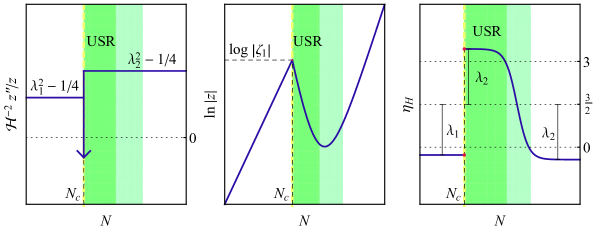
Figure 2: Sketches of $\mathcal{H}^{-2}z^{\prime\prime}/z$ from (3.1), $z$ from (3.2), and $\eta_{H}\approx 1-\partial_{N}\ln|z|$ in the instantaneous T1 transition model. Note that $\mathcal{H}^{-2}z^{\prime\prime}/z$ stays constant throughout USR and afterwards, even though $z$ and $\eta_{H}$ exhibit non-trivial features. The colour coding of vertical bands is the same as in Fig. 1.

We now move to solve the MS equation (2.6) with the ansatz (3.1). The general solution is

$$u_{k}=\left\{\begin{array}[]{ll}\frac{\sqrt{\pi}}{\sqrt{\mathcal{H}}2\sin(\pi\lambda_{1})}\left[c_{1+}J_{-\lambda_{1}}\left(k/\mathcal{H}\right)+c_{1-}J_{\lambda_{1}}\left(k/\mathcal{H}\right)\right]\,,&\quad N<N_{c}\\ \frac{\sqrt{\pi}}{\sqrt{\mathcal{H}}2\sin(\pi\lambda_{2})}\left[c_{2+}J_{-\lambda_{2}}\left(k/\mathcal{H}\right)+c_{2-}J_{\lambda_{2}}\left(k/\mathcal{H}\right)\right]\,,&\quad N>N_{c}\\ \end{array}\right.\,,$$ (3.6)

where $J_{\lambda}$ is a Bessel function of the first kind. The Bunch-Davies vacuum implies $|c_{1+}|=1$, $c_{1-}=-e^{-i\pi\lambda_{1}}c_{1+}$, and the coefficients $c_{2\pm}$ are determined by demanding continuity of $u_{k}$ at $N_{c}$ and setting $u_{k}^{\prime}$ to jump there as determined by the delta function in (3.1). The coefficients can be expressed as

$$\frac{c_{2\pm}}{\zeta_{2}} =\left.\mp\frac{\pi\lambda_{2}}{\zeta_{1}}J_{\pm\lambda_{2}}H_{\lambda_{1}}+\frac{\pi}{\zeta_{2}}\frac{k}{2\mathcal{H}_{c}}\left(\pm J_{\pm\lambda_{2}}H_{\lambda_{1}-1}+J_{\pm\lambda_{2}\pm 1}H_{\lambda_{1}}\right)\right|_{N=N_{c}}\,,$$ (3.7)

where we defined $\mathcal{H}_{c}\equiv\mathcal{H}(N_{c})$, omitted the argument $k/\mathcal{H}_{c}$ of the Bessel and Hankel functions $J_{\lambda}$ and $H_{\lambda}$, and neglected an unimportant phase.

The power spectrum is computed at super-horizon scales where $k\ll\mathcal{H}$ so the Bessel functions in (3.6) can be approximated with their asymptotic forms. Thus, only the coefficient of the growing mode $c_{2+}$ enters and the power spectrum reads

$$\mathcal{P}_{\mathcal{R}} =\frac{k^{3}}{2\pi^{2}}|\mathcal{R}_{c}|^{2}=\frac{k^{2}\Gamma(\lambda_{2})^{2}}{4\pi^{3}}\left|\frac{c_{2+}}{\zeta_{2}}\right|^{2}\left(\frac{k}{2He^{N_{c}}}\right)^{1-2\lambda_{2}}$$ (3.8)

$$=\frac{k^{2}}{4\pi}\Bigg{|}-\frac{\Gamma(1+\lambda_{2})}{\zeta_{1}}\left(\frac{k}{2\mathcal{H}_{c}}\right)^{-\lambda_{2}+1/2}J_{\lambda_{2}}H_{\lambda_{1}}$$

$$\qquad\quad+\frac{\Gamma(\lambda_{2})}{\zeta_{2}}\left(\frac{k}{2\mathcal{H}_{c}}\right)^{-\lambda_{2}+3/2}\left(J_{\lambda_{2}}H_{\lambda_{1}-1}+J_{\lambda_{2}+1}H_{\lambda_{1}}\right)\Bigg{|}_{N=N_{c}}^{2}\,.$$

The first bracketed term is rapidly damped as $k^{-\lambda_{2}-1/2}$ when $k\gg\mathcal{H}_{c}$ and thus it contributes mainly to the $k\ll\mathcal{H}_{c}$ power spectrum generated during the initial SR phase, indicating that the $\mathcal{P}_{\mathcal{R}}$ peak comes from the second term. Its asymptotic behaviour there gives the slope of the power spectrum during SR. Analogously, the asymptotic limits $k\gg\mathcal{H}_{c}$ and $k\ll\mathcal{H}_{c}$ in the second term give the slopes of the peak away from the top. The dominant contributions to the slopes of the power spectrum can thus be summarized as

$$\mathcal{P}_{\mathcal{R}}\propto\left\{\begin{array}[]{ll}k^{3-2\lambda_{1}}\,,&\quad k\lesssim\mathcal{H}_{c}\\ k^{5-2|\lambda_{1}-1|}\,,&\quad\mathcal{H}_{c}\lesssim k\lesssim\mathcal{H}_{c}e^{N_{\rm USR}}\\ k^{3-2\lambda_{2}}\,,&\quad\mathcal{H}_{c}e^{N_{\rm USR}}\lesssim k\end{array}\right.\,.$$ (3.9)

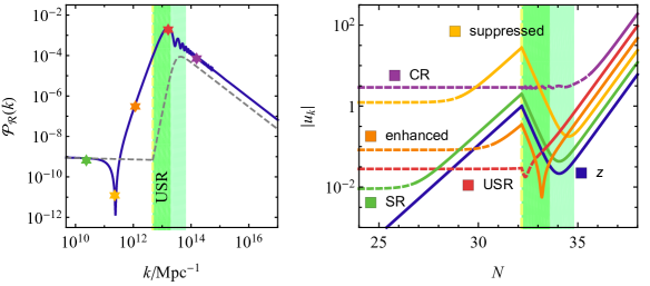
Figure 3: Left panel: The curvature power spectrum (3.8) in the instantaneous transition approximation for the benchmark model #1 from table 1 (blue) and, for comparison, the SR approximation $\mathcal{P}_{\mathcal{R}}=H^{2}/(8\pi^{2}M_{\rm P}^{2}\epsilon_{H})$ with $\epsilon_{H}=z^{2}/(2M_{\rm P}^{2}a^{2})$ (dashed grey), with a number of modes from different regions highlighted. Right panel: Evolution of the Sasaki-Mukhanov variable $u_{k}$ for the corresponding wave numbers from (3.6). The dashed and solid sections correspond to the sub- and super-horizon regions, $\mathcal{H}<k$ and $\mathcal{H}>k$, respectively. The modes are normalized so that their large $N$ asymptotic is the same order as $z$, which in turn is normalized as $z(N_{c})=1$. The colour coding of vertical bands is the same as in Fig. 1.

For small and large $k$, (3.9) gives a scale invariant spectrum if $\lambda_{1,2}=3/2$, corresponding to a pure de Sitter case, while $\lambda_{1,2}>3/2$ ($\lambda_{1,2}<3/2$) will produce a red-tilted (blue-tilted) power spectrum. The peak’s rising slope is sensitive to the behaviour at $N<N_{c}$ through $\lambda_{1}$. As long as $\eta_{H}<0$ during the SR phase, that is, $\lambda_{1}>3/2$ from (3.4), the growth exponent has a maximal value of $4$, consistent with previous studies [156, 157]. In case the spectrum is blue-tilted during the initial phase, i.e., $1<\lambda_{1}<3/2$, the power spectrum can grow as fast as $\mathcal{P}_{\mathcal{R}}\propto k^{5}$, which is similar to the maximal growth $\mathcal{P}_{\mathcal{R}}\propto k^{5}\log^{2}k$ found in Ref. [157].

The position and height of the maximum of the power spectrum (3.8) are given by

$$k_{\rm max}=\mathcal{O}(3)\mathcal{H}_{c}\,,\qquad\mathcal{P}_{\mathcal{R}}(k_{\rm max})=\mathcal{O}(0.05)/\zeta_{2}^{2}\,,$$ (3.10)

respectively. This estimate has only a mild dependence on $\lambda_{2}$, and is almost independent of $\lambda_{1}$. Importantly, note that the position of the maximum depends only on the comoving horizon scale $\mathcal{H}_{c}$ at the T1 phase, while the height of the peak depends on $\zeta_{2}$ and thus, by Eq. (3.3), on the duration of USR. This is expected, because the features of the peak in the spectrum (3.8) arise from the coefficient $c_{+}$ determined by matching of the modes at $N_{c}$, that is, the shape of the peak is determined by mode evolution during T1 phase.

An example of the power spectrum (3.8) is displayed in Fig. 3. The right panel shows the evolution of the $u_{k}$ modes exiting the horizon at different times. Modes that exit much before or after the USR freeze almost immediately after horizon exit. That is, they follow $z$ so that $\mathcal{R}=u_{k}/z={\rm const.}$ (see the discussion in sections 2.2 and 2.3). Modes that exit during or close to USR deviate from $z$ for some time after horizon crossing, briefly following the second solution $u^{(2)}_{0}$ in (2.9), which dominates during USR. At $N_{c}$, we can see the kicks due to the delta function in (3.1). Both $u_{k}$ and $z$ have a tendency to grow, and the growth of the curvature perturbation $|\mathcal{R}_{c\,k}|=\left\lvert u_{k}/z\right\rvert$ during USR is due to the decrease in $z$ rather than the growth of $u_{k}$. Indeed, all the modes depicted in Fig. 3 (except the CR mode that exits well after USR) decrease at least momentarily during USR.

Note the super-horizon enhancement of modes that exit a few $e$-folds before the USR phase, at a time when the SR conditions still hold. The power spectrum in the SR approximation (2.10) is shown in the left panel of Fig. 3 for comparison—while the SR approximation would predict a flat spectrum before the USR phase, the MS equation shows rapid growth. The power spectrum is also mildly enhanced during the final CR phase when compared to the naive SR expectation.

3.1 Potentials producing instantaneous SR to USR transitions

As we will show in this section, the behaviour (3.1) of $\mathcal{H}^{-2}z^{\prime\prime}/z$ can be realized by a scalar field rolling down a potential consisting of two concave parabolas, sketched in Fig. 4,

$$V=\left\{\begin{array}[]{ll}V_{2}\quantity(1+\frac{1}{2M_{\rm P}^{2}}\eta_{V2}\quantity(\phi-\phi_{2})^{2})\,,&\quad\phi<\phi_{c}\phantom{\bigg{|}}\\ V_{1}\quantity(1+\frac{1}{2M_{\rm P}^{2}}\eta_{V1}\quantity(\phi-\phi_{1})^{2})\,,&\quad\phi>\phi_{c}\phantom{\bigg{|}}\end{array}\right.\,.$$ (3.11)

Here $\eta_{V1},\eta_{V2}<0$ are the potential SR parameters $\eta_{V}$ at the two hilltops at $\phi_{1}$ and $\phi_{2}$. We set $\phi_{2}<\phi_{c}<\phi_{1}$ and choose $V_{1}>V_{2}$. The transition point $\phi_{c}$ is at the intersection of the two parabolas so that the potential is continuous. We further choose the parameters so that $V(0)=0$.

During its evolution, the field starts close to the higher hilltop, at $\phi\lesssim\phi_{1}$, rolls down to the sharp feature at $\phi_{c}$, and continues rolling along the other parabola, crossing the lower hilltop at $\phi_{2}$ and continuing towards $\phi=0$. We require $\epsilon_{V}\ll 1$ during this evolution; this is possible if both of the hilltops are sufficiently close to $\phi_{c}$. In this limit, $\epsilon_{H}\ll 1$ for the full duration, and $H$ is approximately a constant, say, $H\approx\sqrt{V_{2}/3}/M_{\rm P}$, as is $\eta_{V}$ separately on the two parabolas. We will use these approximations repeatedly throughout this section. We also take $|\eta_{V1}|<1$, so that the field starts in SR. The SR approximation is only broken at $\phi_{c}$, where $\eta_{V}$ has a negative delta spike. Comparing this to (2.7) and using all the above-mentioned approximations, including $\epsilon_{H}\ll 1$, we see that $z^{\prime\prime}/z$ matches the approximation (3.1) with

$$\lambda_{i}\approx\frac{3}{2}\sqrt{1-\frac{4}{3}\eta_{Vi}}\,,\qquad i=1,2\,,$$ (3.12)

consistent with Eq. (2.16).

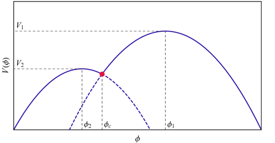
Figure 4: A sketch of the instantaneous transition model potential (3.11).

Let us next study the field’s evolution more closely. In the process, we will make contact with the rest of the formalism presented in section 3.

Near the first hilltop, the field first traverses from an initial value $\phi_{*}$ to the transition point $\phi_{c}$ in SR. The duration of this phase in $e$-folds is approximately

$$N\approx\int_{\phi_{c}}^{\phi_{*}}\frac{\differential\phi}{M_{\rm P}\sqrt{2\epsilon_{V}}}\approx\frac{1}{|\eta_{V1}|}\ln\frac{\Delta\phi_{1}}{\phi_{1}-\phi_{*}}\,,$$ (3.13)

where we defined $\Delta\phi_{i}\equiv|\phi_{i}-\phi_{c}|$. After SR ends, the field continues to evolve in the general way outlined in section 2.3. Analogously to the Eq. (2.15), the field obeys

$$\partial^{2}_{N}\phi+3\partial_{N}\phi+3\eta_{V2}\quantity(\phi-\phi_{2})=0\,,$$ (3.14)

and thus

$$\phi-\phi_{2}=c_{+}e^{(-\frac{3}{2}+\lambda_{2})\quantity(N-N_{c})}+c_{-}e^{(-\frac{3}{2}-\lambda_{2})\quantity(N-N_{c})}\,,$$ (3.15)

where we used (3.12). Note that $z=a\partial_{N}\phi$, and (3.15) is indeed consistent with the $z$ approximation (3.2). The coefficients $c_{\pm}$ are fixed by demanding that $\phi=\phi_{c}$ and $N=N_{c}$ and that the field velocity is continuous. Using the approximation $\partial_{N}\phi_{c}\approx-M_{\rm P}\sqrt{2\epsilon_{V}}\approx\eta_{V1}\Delta\phi_{1}$ on the SR side, we find

$$c_{\pm}=\frac{1}{2\lambda_{2}}\left(\mp|\partial_{N}\phi_{c}|+\Delta\phi_{2}(\pm 3/2+\lambda_{2})\right)\,.$$ (3.16)

Comparing (3.15) to the $z$ approximation (3.2) then gives

$$\frac{\zeta_{2}}{\zeta_{1}}=\frac{\lambda_{2}-3/2}{2\lambda_{2}}\quantity(1-(3/2+\lambda_{2})\frac{\Delta\phi_{2}}{|\partial_{N}\phi_{c}|})\,.$$ (3.17)

Eqs. (3.12) and (3.17) relate the instantaneous transition ansatz (3.2) for $z$ to the piecewise smooth potential (3.11). This correspondence holds up to shifts in $\phi$. The height of the resulting power spectrum $\mathcal{P}_{\mathcal{R}}$ can be changed by changing the height of the potential and thus $H$. This corresponds to rescaling $\zeta_{1}$ in (3.8).

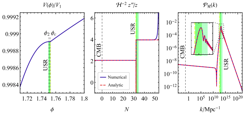
Figure 5: The potential (left panel), $\mathcal{H}^{-2}z^{\prime\prime}/z$ from (2.7) (middle panel), and the power spectrum (right panel) for the potential (3.11) with the parameter values from table 1 (model #1). The blue curves correspond to the full numerical solution with the potential (3.11), whereas the red, dashed curves correspond to the analytical approximations (3.1), (3.8) with parameters determined from (3.12), (3.17). The colour coding of vertical bands is the same as in Fig. 1, and the CMB scales have been marked where appropriate. Notice that the potential is shown only close to the feature at $\phi_{c}$. In the middle panel, the $x$-axis marks the number of $e$-folds from the CMB. The inset highlights that the potential (3.11) perfectly reproduces the oscillations at the $\mathcal{P}_{\mathcal{R}}$ peak found in the approximation (3.8).

In the limit of small $\eta_{V2}$, the length of the USR period (3.3) can be written to leading order as

$$\Delta N_{\rm USR}\approx\frac{1}{3}\ln\frac{6}{-\eta_{V2}\quantity(1-\frac{3\Delta\phi_{2}}{|\partial_{N}\phi_{c}|})}\,.$$ (3.18)

Substituting this to (3.15), the $\phi$-value at the end of USR is, to leading order,

$$\phi_{\rm CR}\approx\phi_{2}+c_{+}\approx\phi_{c}-|\partial_{N}\phi_{c}|/3\,.$$ (3.19)

Since $c_{+}<0$, this is located at a field value somewhat smaller than the lower hilltop $\phi_{2}$. At this level of approximation, the result agrees with pure USR, where the potential term in (3.14) is neglected and the field is left to roll on a plateau until it stops after traversing a field range of $|\partial_{N}\phi_{c}|/3$. If $\eta_{V2}$ is not small, $\phi_{\rm CR}$ can still be solved similarly, but the expressions become lengthy.

The USR phase transitions to CR, where it stays until inflation ends close to $\phi=0$. The remaining number of $e$-folds is approximately [198]

$$\Delta N_{\rm CR} \approx(1-\eta_{H}/3)\int_{0}^{\phi_{\rm CR}}\frac{\differential\phi}{M_{\rm P}\sqrt{2\epsilon_{V}}}$$ (3.20)

$$=\quantity(\frac{1}{2}+\frac{1}{3}\lambda_{2})\quantity[-\frac{1}{\eta_{V2}}\ln\frac{\phi_{2}}{\phi_{2}-\phi_{\rm CR}}-\frac{\phi_{2}^{2}-(\phi_{2}-\phi_{\rm CR})^{2}}{4M_{\rm P}^{2}}]\,,$$

where we dropped the constant $H$ approximation, which breaks down after the field leaves the lower hilltop, but retained the CR assumption of a constant $\eta_{H}$. This concludes our description of the inflaton’s time evolution.

The potential (3.11) can be considered a generalization of the Starobinsky model [164], built out of two linear sections with different slopes. Both models exhibit a similar discontinuity in the first derivative of the potential. Indeed, if we set $\phi_{2}>\phi_{c}$, so that the potential grows monotonously all the way to $\phi_{1}$, the resulting dynamics would be similar to the Starobinsky case near $\phi_{c}$. However, Starobinsky’s scenario cannot support a prolonged period of USR. For that, we need $\phi_{2}<\phi_{c}$ so that the potential has a secondary maximum, slowing the field down as it rolls over the hilltop. We remark that analogous simplified models involving piecewise quadratic potentials have been used to construct analytic descriptions of preheating in plateau inflation [199].

3.2 Constructing potentials for PBHs of any mass

Using the results of the previous sections, we can now tailor a potential to produce PBHs with a desired mass and abundance, simultaneously with desired CMB observables. The full SR parameters of the potential (3.11) read

$$\epsilon_{V}=\frac{\frac{1}{2M_{\rm P}^{2}}\quantity(\phi-\phi_{i})^{2}\eta_{Vi}^{2}}{\quantity(\frac{1}{2M_{\rm P}^{2}}\quantity(\phi-\phi_{i})^{2}\eta_{Vi}+1)^{2}}\,,\qquad\eta_{V}=\frac{\eta_{Vi}}{\frac{1}{2M_{\rm P}^{2}}\quantity(\phi-\phi_{i})^{2}\eta_{Vi}+1}\,,$$ (3.21)

where $i=1$ for $\phi>\phi_{c}$ and $i=2$ for $\phi<\phi_{c}$. Starting from the desired values for $n_{s}$ and $r$, presented in terms of the SR variables in (2.11), we can solve $\eta_{V1}$ and $\phi_{\rm CMB}-\phi_{1}$ from (3.21), where $\phi_{\rm CMB}$ is the CMB field value. Fixing $A_{s}$ then sets $V_{1}$ through (2.10) using $H^{2}=V/(3M_{\rm P}^{2})$ and $\epsilon_{H}\approx\epsilon_{V}$. The desired PBH mass gives the position of the power spectrum peak from (5.4) below with $\Delta N\approx\Delta\ln k$ as $e$-folds from the CMB. The peak will be located roughly at the transition scale $N=N_{c}$, so Eq. (3.13) with $\phi_{*}=\phi_{\rm CMB}$ sets $\phi_{c}$. The parameters $\eta_{V2}$ and $\Delta\phi_{2}$ can then be used to adjust the height of the power spectrum peak and the remaining number of $e$-folds of inflation, setting the PBH abundance and the total length of inflation. The length of USR (3.18) can be a useful proxy for the abundance, and is mainly sensitive to $\Delta\phi_{2}$. In turn, $\eta_{V2}$ controls the remaining number of $e$-folds, approximated by (3.20). The remaining parameters in (3.11), that is, $V_{2}$ and $\phi_{2}$, are fixed by the requirements of continuity at $\phi_{c}$ and the requirement $V(0)=0$.

Model	i	$V_{i}/M_{P}^{4}$	$\eta_{Vi}$	$\phi_{i}$	$\phi_{c}$	$\phi_{\mathrm{CMB}}$
#1	1	$3.1100369\times 10^{-12}$	$-0.017475$	$2.10607$	$1.75215$	$1.9038$
	2	$3.1066362\times 10^{-12}$	$-0.652743$	$1.75043$
#2	1	$3.1100369\times 10^{-12}$	$-0.017475$	$2.62987$	$2.35685$	$2.4276$
	2	$3.1080125\times 10^{-12}$	$-0.360486$	$2.35543$

Model	$n_{s}$	$r$	$N_{\text{CMB}}$	$k_{\text{peak}}$ (Mpc-1)	$\mathcal{P}_{\mathcal{R}}{}_{\text{peak}}$	$M_{\text{PBH}}$ (g)
#1	$0.965$	$0.99\times 10^{-4}$	$53.7$	$1.64\times 10^{13}$	$0.0025$	$1.04\times 10^{20}$
#2	$0.965$	$0.99\times 10^{-4}$	$55.6$	$5.35\times 10^{6}$	$0.014$	$9.75\times 10^{32}$

Table 1: Input parameters and the resulting cosmological observables for the potential (3.11) in two example cases, corresponding to PBHs of approximately $10^{20}$g (model #1) and a solar mass (model #2). For the input parameters, no digits have been omitted: the observables were computed with these exact values. Tuning $\mathcal{P}_{\mathcal{R}}{}_{\text{peak}}$ more finely requires more accuracy in the inputs. The CMB parameters fit the observational constraints [153].

We carried out this exercise and produced two example models, compatible with the CMB observations (2.12) and tuned to produce PBHs with masses $10^{20}$ and $10^{33}$g. We used the analytical expressions in section 3.1 to fix the CMB and as a starting point for tuning the power spectrum peak, but solved the background evolution numerically starting from the potential (3.11), and numerically optimized the parameters $\Delta\phi_{1}$, $\Delta\phi_{2}$, and $\eta_{V2}$. The observables are listed in table 1, given the analytical power spectrum (3.8). The input parameters for the spectrum were computed from the potential using Eqs. (3.12) and (3.17). The resulting parameter values for the potential are listed in table 1. We then solved the MS equation (2.6) numerically for approximately $2000$ modes in model #1 and compared to the analytical approximation. The results are depicted in Fig. 5 and show an excellent match between the analytics and the numerics.

The power spectrum shown in Fig. 5 is typical for a PBH model and, due to its easy-to-manipulate analytical form and a clear connection to a potential, can be used as a proxy for studying observational signals of such models. The only potentially unrealistic feature of the spectrum are the oscillations near the peak, originating from the Bessel functions in (3.8), and induced by the discontinuity at $N_{c}$. In the next section, we modify the model to reduce the amplitude of these oscillations.

4 Approximating the spectra of smooth potentials

The instantaneous transition model of the previous section has two shortcomings: first, it produces a spectrum with a constant spectral index in the SR region, which tends to not capture well the spectrum all the way from the CMB to the PBH scale in smooth models such as those depicted in Fig. 1. Second, it exhibits sharp oscillations in the power spectrum peak, absent in the smooth models. In this section, we attempt to overcome these flaws and approximate the spectra of such smooth models analytically. Fig. 6 shows the resulting example fits.

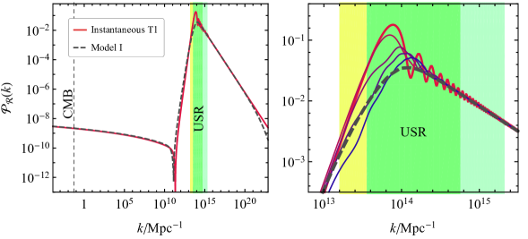
Figure 6: Model I from figure 1 compared to the approximation in Eq. (4.3). On the right hand side, fits using the non-instantaneous transition model are also plotted with varying durations of the T1 phase, $\Delta N_{\rm T}=\{0.5,1,1.5,2\}$ $e$-folds from top to bottom. The remaining parameters were chosen to match the slopes of the peak. The colour coding of vertical bands indicating different inflationary phases is the same as in Fig. 1.

4.1 Fitting the instantaneous transition approximation

To apply the instantaneous transition approximation to realistic models of inflation, we will express the spectrum (3.8) in terms of SR parameters. In the $k\ll\mathcal{H}_{c}$ and $k\gg\mathcal{H}_{c}e^{N_{\rm USR}}$ asymptotics of Eq. (3.8) we find that the power spectrum can be approximated by

$$\mathcal{P}_{\mathcal{R}}^{(\rm CR)}(k;\lambda_{i})\equiv\left.\frac{\Gamma(\lambda_{i})^{2}}{2^{4-2\lambda_{i}}\pi^{3}}\frac{H^{2}}{M_{\rm P}^{2}\epsilon_{H}}\right|_{k=\mathcal{H}},$$ (4.1)

that is, by the usual CR power spectrum [200, 201, 202]. The SR approximation is recovered by $\mathcal{P}_{\mathcal{R}}^{(\rm SR)}(k)\equiv\mathcal{P}_{\mathcal{R}}^{(\rm CR)}(k;3/2)$. In this region, the modes stop evolving after horizon exit, so the usual matching $k=\mathcal{H}$ can be performed. In this way, it is possible to account for an evolving $H$ during the initial SR phase, going beyond the constant $H$ approximation of the previous section. If the $\mathcal{P}_{\mathcal{R}}$ peak is due to a small local maximum in the potential, the $\lambda_{2}$ can be read off from the potential using Eq. (3.12). During the final CR phase, we can fix the normalization of the second term in (3.8) at some fixed scale $k_{\rm CR}$ from the analytic CR power spectrum (4.1). Assuming that the SR approximation is valid during the initial phase, we can choose $\lambda_{1}=3/2$. We can then write down an improved version of (3.8) as

$$\mathcal{P}_{\mathcal{R}}\approx\Bigg{|}\theta(\mathcal{H}_{c}-k)\sqrt{\mathcal{P}_{\mathcal{R}}^{(\rm SR)}}|_{\mathcal{H}=k}+\frac{k\,p(k/\mathcal{H}_{c},\lambda_{2})}{k_{\rm CR}\,|p(k_{\rm CR}/\mathcal{H}_{c},\lambda_{2})|}\sqrt{\mathcal{P}_{\mathcal{R}}^{(\rm CR)}(k_{\rm CR};\lambda_{2}})\Bigg{|}^{2}\,,$$ (4.3)

where

$$p(\kappa;\lambda_{2})\equiv e^{i\kappa}\left(\frac{\kappa}{2}\right)^{1-\lambda_{2}}\left(-J_{\lambda_{2}}\left(\kappa\right)+\left(i-\frac{1}{\kappa}\right)J_{\lambda_{2}+1}\left(\kappa\right)\right)$$ (4.4)

describes the peak generated in the instantaneous SR to USR transitions (we expanded $H_{\lambda_{1}}$ and $H_{\lambda_{1}-1}$ from (3.7) with $\lambda_{1}=3/2$). The step function $\theta$ in the first term models the $k\gg\mathcal{H}_{c}$ damping of the first term in Eq. (3.8). As a fit to a realistic model, (4.3) is fully determined by the evolution of background quantities solved from (2.2), in particular $H$ and the SR parameters $\epsilon_{H}$ and $\eta_{H}$, together with the transition point given by $\mathcal{H}_{c}$. We remark that Eq. (4.3) may be improved further by modifying the shape of $p(\kappa;\lambda_{2})$.

In Fig. 6, the approximation (4.3) is compared to the spectrum from a smooth theoretically well-motivated potential—Model I of Fig. 1, non-minimal quartic inflation (see appendix A for details). For this potential, $\lambda_{2}=1.916$. Apart from the oscillations at the peak, the instantaneous transition approximation (4.3) provides a good model of peaked spectra, fitting both the SR and CR regions well.

In single-field inflation, a degree of tuning is typically required to obtain the desired height of the power spectrum peak. Eq. (4.3) can help with this by providing an approximate analytic representation of the power spectra. In this case, the tuning of the potential parameters to several significant digits can be circumvented as the duration of $\Delta N_{\rm USR}$, or equivalently, the height of the $\mathcal{P}_{\mathcal{R}}$ peak can be set by hand. The rest of the spectrum in (4.3) can be estimated using the SR and CR approximations to obtain $\epsilon_{H}$. This method is relatively fast and can be useful, especially in inflationary model building or GW phenomenology when the relevant observables (e.g., $r$ and $n_{s}$) are relatively insensitive to small changes in the height of the $\mathcal{P}_{\mathcal{R}}$ peak. On the other hand, the approximation (4.3) does not capture the shape of the peak perfectly and is not suitable for precision estimates of the PBH abundance, which can be sensitive to minor adjustments in the peak. We will return to this issue in section 5.1.

4.2 Non-instantaneous SR to USR transitions

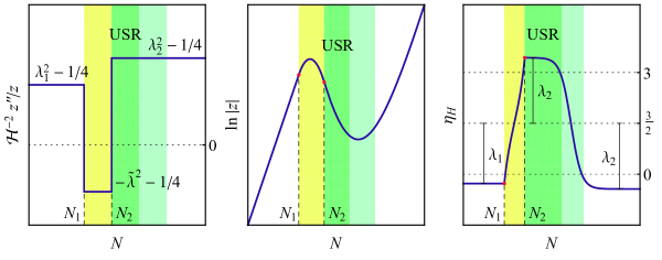
Figure 7: Sketches of $\mathcal{H}^{-2}z^{\prime\prime}/z$ from (4.5), $z$ from (4.6), and $\eta_{H}\approx 1-\partial_{N}\ln|z|$ in the model with non-instantaneous transitions. The colour coding of vertical bands matches Fig. 1

Although the instantaneous transition approximation captures many of the features of the peak in $\mathcal{P}_{\mathcal{R}}$, it produces oscillations around the peak that are not observed with non-singular inflaton potentials. In the following, we will show that this modulation is an artefact of the infinitely sharp transition and can be softened. Similar oscillations in $\mathcal{P}_{\mathcal{R}}$ have been observed when considering inflationary cosmologies with sharp jumps in $\eta_{H}$ and, in a recent work, they have been shown to disappear once the jumps are smoothed [162].

Instead of an instantaneous kick as in Eq. (3.1), let us then consider an intermediate T1 phase lasting $\Delta N_{\rm T}\equiv N_{2}-N_{1}$ $e$-folds. This scenario can be modelled by the ansatz

$$\mathcal{H}^{-2}\frac{z^{\prime\prime}}{z}=\left\{\begin{array}[]{ll}\lambda_{1}^{2}-1/4,&\quad N<N_{1}\\ -\tilde{\lambda}^{2}-1/4,&\quad N_{1}<N<N_{2}\\ \lambda_{2}^{2}-1/4,&\quad N>N_{2}\end{array}\right.\,,$$ (4.5)

where the tilde marks quantities during the T1 phase and $\lambda_{1,2}$ have the same interpretation as in the instantaneous case. The background evolution must now be divided into three epochs,

$$z=\left\{\begin{array}[]{ll}\zeta_{1}e^{(\lambda_{1}-\frac{1}{2})(N-N_{1})},&\quad N<N_{1},\\ \tilde{\zeta}_{+}e^{(i\tilde{\lambda}-\frac{1}{2})(N-N_{1})}+\tilde{\zeta}_{-}e^{(-i\tilde{\lambda}-\frac{1}{2})(N-N_{1})},&\quad N_{1}<N<N_{2},\\ \zeta_{2+}e^{(\lambda_{2}-\frac{1}{2})(N-N_{2})}+\zeta_{2-}e^{(-\lambda_{2}-\frac{1}{2})(N-N_{2})}&\quad N_{2}<N,\end{array}\right.$$ (4.6)

where the coefficients $\zeta_{i}$ are given in appendix B. An example of $z$ evolution (4.6) is shown in Fig. 7. This should be compared to Fig. 2: the sharp features in the instantaneous transition have been eliminated. Setting the end of USR to the point where $\eta_{H}=1$, the duration of the USR phase is

$$\Delta N_{\rm USR}\approx\frac{1}{2\lambda_{2}}\ln\quantity[\frac{\lambda_{2}+1/2}{\lambda_{2}-1/2}\frac{\zeta_{2-}}{\zeta_{2+}}]\,.$$ (4.7)

Noting that in the instantaneous case $\zeta_{2-}=\zeta_{1}-\zeta_{2+}$, this expression is identical to Eq. (3.3). An extended USR period is realized when the growing mode is strongly suppressed at the beginning of the USR phase, i.e., $|\zeta_{2+}|\ll|\zeta_{2-}|$.

Analogously, the general solution to the MS equation now reads

$$u_{k}=\left\{\begin{array}[]{ll}\frac{\sqrt{\pi}}{\sqrt{\mathcal{H}}2\sin(\pi\lambda_{1})}\left[c_{1+}J_{-\lambda_{1}}\left(\frac{k}{\mathcal{H}}\right)+c_{1-}J_{\lambda_{1}}\left(\frac{k}{\mathcal{H}}\right)\right]\,,&\quad N<N_{1}\\ \frac{\sqrt{\pi}}{\sqrt{\mathcal{H}}2\sin(\pi i\tilde{\lambda})}\left[\tilde{c}_{+}J_{-i\tilde{\lambda}}\left(\frac{k}{\mathcal{H}}\right)+\tilde{c}_{-}J_{i\tilde{\lambda}}\left(\frac{k}{\mathcal{H}}\right)\right]\,,&\quad N_{1}<N<N_{2}\\ \frac{\sqrt{\pi}}{\sqrt{\mathcal{H}}2\sin(\pi\lambda_{2})}\left[c_{2+}J_{-\lambda_{2}}\left(\frac{k}{\mathcal{H}}\right)+c_{2-}J_{\lambda_{2}}\left(\frac{k}{\mathcal{H}}\right)\right]\,,&\quad N_{2}<N\end{array}\right.\,,$$ (4.8)

with the expressions for the coefficients $c_{i}$ listed in appendix B. The power spectrum is again determined from the coefficient $c_{2+}$ of the growing mode,

$$\mathcal{P}_{\mathcal{R}}=\frac{k^{3}}{2\pi^{2}}|\mathcal{R}_{c}|^{2}=\frac{k^{2}\Gamma(\lambda_{2})^{2}}{4\pi^{3}}\left|\frac{c_{2+}}{\zeta_{2+}}\right|^{2}\left(\frac{k}{2\mathcal{H}_{2}}\right)^{1-2\lambda_{2}}\,,$$ (4.9)

where $\mathcal{H}_{2}\equiv\mathcal{H}(N_{2})$. Due to the complicated form of the expressions, we do not study the details of (4.9) further, but we note that the asymptotic behaviour in the SR and CR regions coincides with the instantaneous transition approximation.

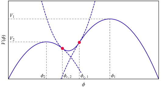
Figure 8: A sketch of the non-instantaneous SR to USR transition model potential (4.10).

Similarly to the instantaneous transition case, we can build a potential that generates the behaviour (4.5). Taking hints from section 3.1, it is clear that the potential should consist of three parabolas: one for the initial SR and another for the final CR phases as before, and one with a positive second derivative to connect them smoothly. We write it as

$$V=\left\{\begin{array}[]{ll}V_{1}\quantity(1+\frac{1}{2}\eta_{V1}\quantity(\phi-\phi_{1})^{2})\,,&\quad\phi_{c,1}<\phi\\ \tilde{V}\quantity(1+\frac{1}{2}\tilde{\eta}_{V}\quantity(\phi-\tilde{\phi})^{2})\,,&\quad\phi_{c,2}<\phi\leq\phi_{c,1}\\ V_{2}\quantity(1+\frac{1}{2}\eta_{V2}\quantity(\phi-\phi_{2})^{2})\,,&\quad\phi\leq\phi_{c,2}\end{array}\right.\,,$$ (4.10)

with $\lambda_{i}$ and $\eta_{Vi}$ related by Eq. (3.12), and $\tilde{\lambda}=(3/2)\sqrt{(4/3)\tilde{\eta}_{V}-1}$. Requiring $\mathcal{H}^{-2}z^{\prime\prime}/z<0$ in the intermediary region corresponds to $\tilde{\eta}_{V}>2/3$. This makes sense: to break the SR approximation, a value of $\eta_{V}$ of order one is required. This time, $\eta_{V}$ has no delta peaks, only discontinuities, and thus the first derivative of the potential must be continuous everywhere. A sketch of the potential is depicted in Fig. 8.

Again, spectra of the form (4.9) can be produced by a potential of the form (4.10). In the intermediary region, a solution similar to (3.15) applies, and the parameters of the $z$ and $V$ functions there can be straightforwardly matched by expressions similar to (3.17), paying attention to the continuity of the field velocity. In principle, even more complicated forms of $\mathcal{H}^{-2}z^{\prime\prime}/z$ and the potential can be built and matched with a similar procedure. The details are not very illuminating, and we will not study them here.

The advantage of the “box” model for non-instantaneous transitions is that it reduces the discontinuity of $\mathcal{H}^{-2}z^{\prime\prime}/z$ and thus dampens the oscillations in the power spectrum peak. An example of this is shown in Fig. 6, where the duration of the transition phase, $\Delta N_{\rm T}=N_{2}-N_{1}$, is varied while fitting the rising and falling slopes of the peak to the smooth Model I. The correct steepness of the slopes was achieved by setting $\lambda_{1}=1.8$ and $\lambda_{2}=1.916$. To fix the position of the falling slope, the end of USR with $z^{\prime}=0$ was matched in the smooth model and in the non-instantaneous approximation. To fix the position of the rising slope, the position of the ‘dip’ in $\mathcal{H}^{-2}z^{\prime\prime}/z$ was varied by hand. The results show that quick transitions mimic the instantaneous approximation, as expected, while widening the transition smoothens the spectrum, but only to a degree. A spurious ‘bump’ remains on top of the smooth spectrum, even for wide transitions, and the bump is further modulated by oscillations arising from the sharp edges at $N_{1}$ and $N_{2}$.

5 Phenomenology

Aided by the analytical expressions for the curvature power spectrum, we will next estimate the abundance of PBHs and GWs induced by the large fluctuations, and consider the constraints from CMB.

5.1 Primordial black holes

High amplitude curvature perturbations lead to formation of PBHs after their horizon re-entry [6, 7, 31]. PBH formation occurs if the smoothed density contrast $\delta_{m}$ exceeds a threshold value $\delta_{c}$ [31, 203, 204, 205, 206, 207, 208, 209]. We estimate the fraction of the total energy density $\beta_{k}(M){\rm d}\ln M$ that collapses into BHs of mass $M$ using the Press-Schechter formalism [210, 211, 31, 212]:

$$\beta_{k}(M)=\int_{\delta_{l,c}}^{\infty}{\rm d}\delta_{l}\,\frac{M}{M_{k}}\,P_{k}(\delta_{l})\delta_{D}\!\left[\ln\frac{M}{M(\delta_{m}(\delta_{l}))}\right]\,,$$ (5.1)

where $\delta_{D}$ denotes the Dirac delta function, $\delta_{l,c}$ is the threshold value of $\delta_{l}$, called the linear Gaussian component in the literature, which is related to the density contrast $\delta_{m}$ via [213, 214, 215, 216]

$$\delta_{m}=\delta_{l}-\frac{3}{8}\delta_{l}^{2}\,,$$ (5.2)

and $P_{k}$ is its probability distribution. Using the critical scaling [217, 218, 219]

$$M(\delta_{m})=\kappa M_{k}\left(\delta_{m}-\delta_{c}\right)^{\gamma}\,,$$ (5.3)

where $\gamma=0.36$ [217, 220] and $M_{k}$ is the horizon mass

$$M_{k}=\frac{4\pi M_{\rm P}^{2}}{H_{k}}\approx 1.4\times 10^{13}M_{\odot}\left(\frac{k}{{\rm Mpc}^{-1}}\right)^{-2}\,\left(\frac{g_{*,s}^{4}g_{*}^{-3}}{106.75}\right)^{-1/6}\,,$$ (5.4)

we can express $\beta_{k}(M)$ as

$$\beta_{k}(M)=\frac{2\kappa}{\gamma}\frac{q^{1+1/\gamma}P_{k}(\delta_{l}(M))}{1-\frac{3}{4}\delta_{l}(M)}\,,$$ (5.5)

where $q\equiv M/(\kappa M_{k})$ and $\delta_{l}(M)$ is the inversion of the critical scaling law (5.3),

$$\delta_{l}(M)=\frac{4}{3}\left[1-\sqrt{1-\frac{3}{2}\left(\delta_{c}+q^{1/\gamma}\right)}\right]\,.$$ (5.6)

The threshold density contrast $\delta_{c}$ and the $\kappa$ parameter depend on how the primordial perturbations are smoothed [221, 222, 212] as well as on the shape of individual peaks [207, 213, 223, 224]. We use $\delta_{c}=0.55$ and $\kappa=4.0$ [213].

We assume that the curvature perturbations are Gaussian,

$$P_{k}(\delta_{l})=\frac{1}{\sqrt{2\pi}\sigma_{k}}\,e^{-\delta_{l}^{2}/2\sigma_{k}^{2}}\,,$$ (5.7)

where $\sigma_{k}$ is the variance at scale $k$. The assumption of Gaussianity introduces potential inaccuracies as the curvature perturbations can develop non-Gaussianities in the form of an exponential tail in the probability distribution (5.7), which can lead the Gaussian expression to underestimate the PBH abundance by several orders of magnitude [225, 226, 227, 106]. The correction is model-dependent and requires a non-linear analysis. There is currently no simple semi-analytical way to compute it accurately. We use (5.7) as a first approximation, keeping in mind that e.g. tuning the power spectrum height slightly can lead to comparable changes in the abundance. Neglecting the contribution of connected correlation functions of the curvature power spectrum [216], the variance of $\delta_{l}$ is obtained from the curvature power spectrum $\mathcal{P}_{\mathcal{R}}(k)$ [213],

$$\sigma_{k}^{2}=\left(\frac{4}{9}\right)^{2}\int_{0}^{\infty}\frac{{\rm d}k^{\prime}}{k^{\prime}}\left(\frac{k^{\prime}}{k}\right)^{\!4}W^{2}(k^{\prime}/k)T^{2}(k^{\prime}/k)\mathcal{P}_{\mathcal{R}}(k^{\prime})\,.$$ (5.8)

Following Ref. [213], we evaluate the variance using a real-space top-hat window function $W(x)=3(\sin x-x\cos x)/x^{3}$, and accounting for the damping of sub-horizon fluctuations with the linear transfer function $T(x)=3[\sin(x/\sqrt{3})-x/\sqrt{3}\cos(x/\sqrt{3})]/(x/\sqrt{3})^{3}$. Finally, the present day PBH mass function, normalised to the PBH abundance, $\int{\rm d}\ln M\psi(M)=\Omega_{\rm PBH}$, is

$$\psi(M) =\int{\rm d}\ln k\,\beta_{k}(M)\frac{\rho_{\gamma}(T_{k})}{\rho_{c}}\frac{s(T_{0})}{s(T_{k})}\,$$ (5.9)

$$\simeq\frac{4\times 10^{-12}}{\gamma}\!\frac{M}{M_{\odot}}\int\!\frac{{\rm d}k\,k^{2}}{{\rm Mpc}^{-3}}\frac{q^{1/\gamma}P_{k}(\delta_{l}(M))}{1-\frac{3}{4}\delta_{l}(M)}\,,$$

where $\rho_{\gamma}(T)$ and $s(T)$ are the radiation energy and entropy densities, and $\rho_{c}$ denotes the critical energy density of the Universe.

Figure 9: The abundance of gravitational waves (left) and primordial black holes (right). The solid curves correspond to $\lambda_{2}=1.916$ as in Fig. 6, the green dashed to $\lambda_{2}=1.8$ and the orange dot-dashed to $\lambda_{2}=3.0$. The latter two correspond to the benchmark cases shown in Fig. 10, and they overlap with the $\Delta N_{T}=0$ curve in the right panel. For each case $\lambda_{1}=1.52$.

Similarly as in Ref. [149], we find that for the curvature power spectrum (3.8), independently of $\lambda_{2}$, the PBH mass function is of the form

$$\psi(M)\propto M^{1+1/\gamma}e^{-c_{1}(M/\langle M_{\rm PBH}\rangle)^{c_{2}}}\,,$$ (5.10)

where $c_{1}$ is fixed such that $\langle M_{\rm PBH}\rangle$ is the average PBH mass, and $c_{2}\simeq 1$ has a mild dependence on the peak amplitude of the curvature power spectrum. The abundance of PBHs and their mean mass are given in terms of the curvature power spectrum peak position $k_{*}$ and amplitude $A_{*}$ by

$$\Omega_{\rm PBH} \simeq c_{\Omega}A_{*}^{c^{\prime}_{\Omega}}\,e^{-c_{A}/A_{*}}\,k_{*}/{\rm Mpc}^{-1}\,,$$ (5.11)

$$\left\langle M_{\rm PBH}\right\rangle \simeq c_{M}A_{*}^{c^{\prime}_{M}}M_{k_{*}}\,,$$

where $c_{\Omega}\approx 30$, $c^{\prime}_{\Omega}\approx 1.3$, $c_{A}\approx 0.4$, $c_{M}\approx 16$ and $c^{\prime}_{M}\approx 0.34$. As shown in the right panel of Fig. 9, a non-instantaneous SR to USR transition only slightly changes the value of $A_{*}$ that gives rise to the particular PBH abundance.

In Fig. 10 we use the spectrum (3.8) for instantaneous SR to USR transitions and plot the projection of the PBH constraints in the plane of the amplitude $A_{*}$ and position $k_{*}$ of the maximum in the curvature power spectrum. The gray region in is excluded by the PBH constraints. These constraints arise from Hawking evaporation during big-bang nucleosynthesis and non-observation of extragalactic gamma-ray background from PBH evaporation [228, 229], microlensing results from Subaru/HSC [12, 230], EROS [231], OGLE [232], Kepler [233] and MACHO [234], GW event rate observed by LIGO-Virgo [22], lensing of type Ia supernovae [235], lensing of LIGO-Virgo events [236], survival of stars in dwarf galaxies [237, 238], survival of wide binaries [239], Lyman-$\alpha$ forest data [240, 241] and limits on accretion [242, 243, 244, 245, 246, 247, 248]. The envelope of these constraints shown by the gray curve is calculated using the method introduced in [249] from the constraints for monochromatic mass functions to the mass function (5.10).

5.2 Gravitational waves

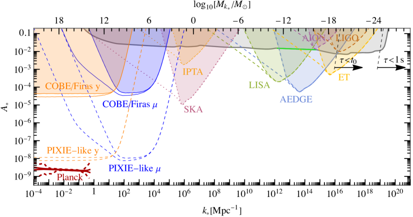
Figure 10: Constraints (solid lines) and projected sensitivities of future experiments (dashed lines) on the peak amplitude $A_{*}$ of the curvature power spectrum as a function of the peak position $k_{*}$ in the case of an instantaneous SR to USR transition. The red solid and dashed lines in the bottom left corner correspond to $1\sigma$ and $3\sigma$ constraints from Planck CMB observations. The gray solid line corresponds to the envelope of the PBH constraints and the green line highlights the asteroid mass window where all DM could be in PBHs. The PBH lifetime $\tau$ is evaluated for the average PBH mass. The parameters of the curvature power spectrum (3.8) are fixed to $\lambda_{1}=1.52$ and two cases for $\lambda_{2}$ are shown: $\lambda_{2}=1.8$ (smaller $A_{*}$ or weaker constraint) and $\lambda_{2}=3.0$ (larger $A_{*}$ or stronger constraint).

Curvature perturbations induce formation of GWs at second order from the mode coupling [137, 138, 139, 140, 141]. Recently, these scalar-induced GWs (SIGWs) have been extensively studied (see for instance [142, 250, 251, 252, 253, 254]), and the prospects for observing them have been considered [165, 166, 167, 168, 169, 170, 171, 172, 156, 173, 174, 175, 176, 177, 178, 255]. SIGWs have been searched for but not detected by the LIGO-Virgo collaboration [143, 144]. However, it has been suggested that the recent NANOGrav result [145] could be explained by SIGWs [149, 150, 151, 152].

During radiation domination, GWs decouple from scalar perturbations soon after horizon crossing and their abundance reaches a constant value. The SIGW spectrum today is given by (see e.g. [250, 251])

$$\Omega_{\rm GW}(k)=0.387\,\Omega_{\rm R}\left(\frac{106.75}{g_{*,s}^{4}g_{*}^{-3}}\right)^{\!\frac{1}{3}}\frac{1}{6}\int_{-1}^{1}\!{\rm d}x\int_{1}^{\infty}\!{\rm d}y\,\mathcal{P}_{\mathcal{R}}\!\left(\frac{x-y}{2}k\right)\mathcal{P}_{\mathcal{R}}\!\left(\frac{x+y}{2}k\right)F(x,y)\,,$$ (5.12)

where $\Omega_{\rm R}=5.38\times 10^{-5}$ is the radiation abundance [261], the effective number of degrees of freedom are evaluated at the moment when the constant abundance is reached, roughly coinciding with the horizon crossing moment, and

$$F(x,y)= \frac{288(x^{2}+y^{2}-6)^{2}(x^{2}-1)^{2}(y^{2}-1)^{2}}{(x-y)^{8}(x+y)^{8}}$$ (5.13)

$$\times\left[\left(x^{2}-y^{2}+\frac{x^{2}+y^{2}-6}{2}\log\left|\frac{y^{2}-3}{x^{2}-3}\right|\right)^{2}\!+\frac{\pi^{2}(x^{2}+y^{2}-6)^{2}}{4}\theta(y-\sqrt{3})\right].$$

In the left panel of Fig. 9 we show the GW spectrum corresponding to the curvature power spectrum (3.8) for three benchmark cases. In each case we have fixed $\lambda_{1}=1.52$ to match the CMB observations, and for $\lambda_{2}$ we consider three values, $1.8$ (green dashed), $1.916$ (solid) and $3.0$ (orange dot-dashed). Moreover, for $\lambda_{2}=1.916$, we consider the GW spectra and PBH abundances for the curvature power spectrum of a non-instantaneous SR to USR transition (4.9) (compare to Fig. (6)).

For a given shape of the peak in the curvature power spectrum, we can project the sensitivities of different GW observatories on the plane of the curvature power spectrum peak position $k_{*}$ and amplitude $A_{*}$. In Fig. 10 we show in two benchmark cases of an instantaneous USR to SR transition, corresponding to $\lambda_{1}=1.52$, $\lambda_{2}=1.8$ and $\lambda_{1}=1.52$ and $\lambda_{2}=3.0$, these projections for IPTA [148], SKA [262] LISA [263], AEDGE [264, 265], AION [266, 265], ET [267] and LIGO [268]. We characterize the detectability of the GW signal by the signal-to-noise ratio

$${\rm SNR}=\sqrt{\mathcal{T}\int{\rm d}f\left[\frac{\Omega_{\rm GW}(f)}{\Omega_{\rm sens}(f)}\right]^{2}}\,,$$ (5.14)

where $\mathcal{T}$ is the observation time and $\Omega_{\rm sens}(f)$ the sensitivity of the given detector. We take $\mathcal{T}=5\,$years and ${\rm SNR}>10$ for the threshold signal-to-noise ratio. By varying $\Delta N_{\rm T}$ in the toy model for non-instantaneous transitions (4.9), we checked that the sensitivities shown in Fig. 10 are only marginally affected by the duration of the transition.

The values $\lambda_{2}=1.8$ and $\lambda_{2}=3.0$ enclose most of the phenomenologically interesting range. For instance, Table 1 together with Eq. (3.12) gives the values $\lambda_{2}=1.83$ and $\lambda_{2}=2.05$—these correspond to spectra with relatively flat $\mathcal{P}_{\mathcal{R}}$ peaks producing solar mass PBHs and steeper peaks required for populating the asteroid mass PBH DM window, respectively. However, the identification $\lambda_{2}$ with the PBH mass is not unique and depends on other features of the inflationary scenario, such as the duration of inflation and whether it ends after the dual USR+CR phase during which the peak is produced (compare, for instance, Model I and Model III in Fig. 1).

5.3 CMB constraints

The CMB observations directly strongly constrain the curvature power spectrum at scales $10^{-4}\,{\rm Mpc}^{-1}\mathrel{\raise 1.29167pt\hbox{$<$\kern-7.5pt\lower 4.30554pt\hbox{$\sim$}}}k\mathrel{\raise 1.29167pt\hbox{$<$\kern-7.5pt\lower 4.30554pt\hbox{$\sim$}}}1\,{\rm Mpc}^{-1}$. In Fig. 10 we show with dark red curves the $1\sigma$ and $3\sigma$ Planck constraints on the evolution of the curvature power spectrum from Ref. [274].

At redshifts $z\lesssim 10^{6}$ energy injections into the primordial plasma cause persisting spectral distortions in the CMB. These distortions are divided into chemical potential $\mu$-type distortions created at early times and Compton $y$-type distortions created at $z\lesssim 5\times 10^{4}$. For a given curvature power spectrum $\mathcal{P}_{\mathcal{R}}(k)$ the $X=\mu,y$ spectral distortions are [180, 181]

$$X=\int_{k_{\rm min}}^{\infty}\frac{{\rm d}k}{k}\,\mathcal{P}_{\mathcal{R}}(k)W_{X}(k)\,,$$ (5.15)

where $k_{\rm min}=1\,{\rm Mpc}^{-1}$ and the window functions can be approximated by

$$W_{\mu}(k)=2.2\left[e^{-\frac{(\hat{k}/1360)^{2}}{1+(\hat{k}/260)^{0.6}+\hat{k}/340}}-e^{-\left(\hat{k}/32\right)^{2}}\right]\,,\qquad W_{y}(k)=0.4e^{-\left(\hat{k}/32\right)^{2}}\,,$$ (5.16)

with $\hat{k}=k/(1\,{\rm Mpc}^{-1})$.

The COBE/Firas observations constrain the $\mu$ and $y$ distortions as $\mu\leq 9\times 10^{-5}$ and $y\leq 1.5\times 10^{-5}$ [179] at $95\%$ CL. These imply strong constraints on the curvature power spectrum in the range $k\lesssim 10^{4}{\rm Mpc}^{-1}$ [180, 181]. Moreover, a PIXIE-like detector could probe distortions as small as $\mu\leq 2\times 10^{-8}$ and $y\leq 0.4\times 10^{-8}$ [275]. We show the COBE/Firas constraints as well as the projections of a PIXIE-like detector sensitivity in Fig. 10 for two benchmark cases of the curvature power spectrum (3.8). We find that the $\mu$-distortion constraints exclude single-field formation of PBHs heavier than $10^{4}M_{\odot}$. Importantly, we find that this constraint is negligibly affected by variations in model parameters.

6 Conclusions

We have considered the general structure of single-field inflationary models capable of producing peaked curvature spectra. We have restricted our study to models in which an Einstein frame exists and the dynamics can be captured by a single function—the Einstein frame potential. In such cases, both numerical and analytic approaches indicate that inflation can be divided into the following epochs:

• Slow-roll. Typically the density fluctuations at the CMB scale are produced in this phase.

• Slow-roll to ultra-slow-roll transition. This phase will involve violation of the slow-roll conditions or even a brief exit from an inflationary cosmology. The power spectrum begins to grow slightly before this phase. The details of this phase vary the most from model to model. For instance, it can be triggered by a small maximum in the potential or by rolling through its global minimum.

• Ultra-slow-roll. The field starts to rapidly lose its velocity either by climbing up a hill in the potential or by rolling down a near plateau. The power spectrum typically reaches its peak during this phase.

• Constant-roll (or also slow-roll). The velocity of the field begins to grow as the field begins to roll down the potential constantly (or slowly). If the potential is continuous, this phase is dual to the previous one and sets the declining slope of the power spectrum peak.

We have omitted a transitory period from ultra-slow-roll to constant-roll from the above list because it is entirely described by the duality of its neighbouring phases. All listed phases are present in single-field inflationary models for PBHs and can contribute to the enhanced curvature power spectrum.

Assuming instantaneous slow-roll to ultra-slow-roll transitions, we have constructed an analytically solvable scenario that accounts for the inherent duality between the consecutive ultra-slow-roll and constant-roll phases. Such transitions can arise from piecewise quadratic potentials. The resulting curvature power spectrum can be consistent with CMB observations and can include a high peak that leads to a significant abundance of PBHs of any mass. The curvature power spectrum in this case oscillates at small scales below the peak. Relying on our analytic estimates, we have devised a simple analytic prescription in Eq. (4.3) that allows to approximate peaked power spectra for general single-field inflationary models.

We have studied how the shape of the peak depends on details of the slow-roll to ultra-slow-roll transition by constructing simplified solvable models in which the duration of this transition can be easily varied. The oscillations found in the case of instantaneous transition get smoother for slower transitions. These models can be considered as limiting cases of smooth physical potentials. In particular, we conclude that, in general single-field models for PBHs, the tails of the peak in the power spectrum can be determined from the potential alone via the second potential slow-roll parameter, while the exact shape of the peak (for instance the presence of oscillating features) depends on the details of how the initial slow-roll phase transitions into the subsequent ultra-slow-roll phase.

We have considered how the shape of the peak in the power spectrum affects the PBH abundance and the related scalar-induced GWs. A firm grasp of this relation is crucial for probing PBH phenomenology via GW observations. We have found that, although the details of the peak shape can affect the PBH abundance by a few orders of magnitude, the prospects for the detection of scalar-induced GWs as well the power spectrum amplitude required for abundant PBH production are quite insensitive to it. Next-generation GW detectors such as LISA and AEDGE are expected to probe the entire asteroid mass window for PBH dark matter. The COBE/Firas $\mu$-distortion constraints exclude the production of PBHs heavier than $10^{4}M_{\odot}$ in single-field inflation.

Appendix A Potentials and parameters for the example models

The inflationary models given as an example in Fig. 1 of section 2 have actions of the form

$$S=\int{\rm d}^{4}x\,\sqrt{-g}\left(\frac{1}{2}M_{\rm P}^{2}\Omega(\sigma)R-\frac{1}{2}K(\sigma)(\partial\sigma)^{2}-V(\sigma)\right)\,,$$ (A.1)

where $\sigma$ is the inflaton, $\Omega(\sigma)$ contains the non-minimal couplings, $K$ accounts for the possibility of a non-canonical kinetic term, $V$ is the potential, $V(v)=0$ at the vacuum with $\sigma=v$, and $M_{\rm P}=2.4\times 10^{18}{\rm GeV}$ is the reduced Planck mass. In the following sections, we specify these functions for the different models. All parameter values are gathered in table 2, and the inflationary observables are presented in table 3. To compute the results, we have performed the appropriate field redefinitions and conformal transformations [276] to eliminate $\Omega$ and $K$ and bring the action back to the standard form (2.1).

A.1 Model I: non-minimal polynomial inflation

This model is defined by

$$V=\frac{1}{2}m^{2}\sigma^{2}+\frac{1}{3}\mu\sigma^{3}+\frac{1}{4}\lambda\sigma^{4},\qquad\Omega=1+\xi\sigma^{2}/M_{\rm P}^{2},\qquad K=1\,,$$ (A.2)

inspired by [54, 58, 59]. The cubic term can be used to create a small maximum in the potential. Following [54], we reparametrize the model in terms of the extrema of the Einstein frame potential $V_{E}\equiv V/\Omega^{2}$ at $\sigma=v_{i}$, $i=1,2,3$, giving

$$m^{2}=\frac{1}{2}\lambda\frac{v_{2}v_{3}(\xi v_{2}v_{3}+3M_{\rm P}^{2})M_{\rm P}^{2}}{\xi^{2}v_{2}^{2}v_{3}^{2}-\xi(v_{2}-v_{3})^{2}M_{\rm P}^{2}+3M_{\rm P}^{4}}\,,\qquad\mu=-\frac{\lambda(v_{2}+v_{3})M_{\rm P}^{4}}{\xi^{2}v_{2}^{2}v_{3}^{2}-\xi(v_{2}-v_{3})^{2}M_{\rm P}^{2}+3M_{\rm P}^{4}}\,.$$ (A.3)

We use $v_{1}\leq v_{2}\leq v_{3}$, where, by construction, the trivial extremum lies at the origin, $v_{1}=0$. An exact inflection point corresponds to $v_{2}=v_{3}$. The second potential SR parameter at the local maximum $v_{2}$ is

$$\eta_{V,c}=-\frac{4(v_{3}-v_{2})(\xi v_{2}(v_{2}+2v_{3})+3M_{\rm P}^{2})M_{\rm P}^{4}}{v_{2}^{2}\left(\xi(6\xi+1)v_{2}^{2}+M_{\rm P}^{2}\right)\left(2v_{3}M_{\rm P}^{2}-v_{2}\left(M_{\rm P}^{2}-\xi v_{3}^{2}\right)\right)}\,.$$ (A.4)

By Eq.’s (4.1) and (3.12), it gives the high $k$ slope of the $\mathcal{P}_{\mathcal{R}}$ peak. The observables of Fig. 1 are computed in the Einstein frame, with the canonical field $\phi$ solved numerically from

$$\frac{\differential\phi}{\differential\sigma}=\frac{1}{\Omega(\sigma)}\sqrt{\Omega(\sigma)+\frac{3M_{\rm P}^{2}}{2}\quantity(\frac{\differential\Omega(\sigma)}{\differential\sigma})^{2}}\,.$$ (A.5)

Model	Parameters
I	$\lambda=2.10\times 10^{-5}$	$\xi=80.0118$	$v_{2}=0.08M_{\rm P}$	$v_{3}=0.0855714M_{\rm P}$
II	$V_{0}=1.89\times 10^{-10}M_{\rm P}^{4}$	$\alpha=1$	$A=0.130383$	$f_{\sigma}=0.129576$
III	$V_{0}=7.03\times 10^{-11}M_{\rm P}^{4}$	$A=1.17\times 10^{-3}$	$\phi_{0}=2.188M_{\rm P}$	$\Delta=1.59\times 10^{-2}M_{\rm P}$

Table 2: Parameter values for the models I, II, and III plotted in Fig. 1. No digits have been omitted: all numerical computations were performed with these exact values. See sections A.1, A.2, A.3 for the expressions for the potentials.

A.2 Model II: $\alpha$-attractor inflation

This model, from [65], is defined in the setup of superconformal $\alpha$-attractor models, with the inflaton sector given by

$$V=f^{2}\quantity(\frac{\sigma}{\sqrt{3}M_{\rm P}}),\qquad\Omega=1,\qquad K=\frac{2\alpha}{\quantity(1-\frac{\sigma^{2}}{3M_{\rm P}^{2}})^{2}}\,.$$ (A.6)

The kinetic term is canonical for the redefined field

$$\phi=\sqrt{6\alpha}M_{\rm P}\tanh^{-1}\frac{\sigma}{\sqrt{3}M_{\rm P}}\,,$$ (A.7)

and we pick a model with $f(x)=\lambda\quantity(x+A\sin\frac{x}{f_{\sigma}})$ and $\alpha=1$, so that the canonical potential reads

$$V(\phi)=V_{0}\quantity[\tanh\quantity(\frac{\phi}{\sqrt{6}M_{\rm P}})+A\sin\quantity(f_{\sigma}^{-1}\tanh\quantity(\frac{\phi}{\sqrt{6}M_{\rm P}}))]^{2}\,,\qquad V_{0}=\lambda^{2}\,.$$ (A.8)

The sinusoidal modulation produces an inflection point to the otherwise plateau-like potential. In the notation of [65], this is Model II, and we use their parametrization #1, reproduced in table 2.

A.3 Model III: modified KKLT inflation

This model, from [80], is a modified version of the string theory based KKLT inflation, defined by

$$V=V_{0}\frac{\phi^{2}}{(M_{\rm P}/2)^{2}+\phi^{2}}\quantity(1+\epsilon(\phi))\,,\qquad\Omega=1\,,\qquad K=1\,.$$ (A.9)

Gravity and the kinetic term are canonical from the get-go. The base plateau potential is modified by a small Gaussian bump,

$$\epsilon(\phi)=A\,e^{-(\phi-\phi_{0})^{2}/(2\Delta^{2})}\,,$$ (A.10)

and dynamics around this bump enhance the power spectrum. We use one of the parameter sets given in [80].

Model	$n_{s}$	$r$	$N_{\text{CMB}}$	$\phi_{\text{CMB}}/M_{\rm P}$	$k_{\text{peak}}$ (Mpc-1)	$\mathcal{P}_{\mathcal{R}}{}_{\text{peak}}$	$M_{\text{PBH}}$ (g)
I	$0.947$	$0.023$	$56.9$	$6.78$	$1.25\times 10^{14}$	$0.035$	$1.79\times 10^{18}$
II	$0.945$	$0.0075$	$56.7$	$5.85$	$9.09\times 10^{13}$	$0.017$	$3.37\times 10^{18}$
III	$0.968$	$0.0022$	$60.0$	$3.08$	$2.18\times 10^{14}$	$0.0016$	$5.88\times 10^{17}$

Table 3: Inflationary observables for the models I, II, and III. For models II and III, these differ slightly from those reported in the original articles [65] and [80], presumably due to the limited numerical accuracy of the input parameter values given there.

Appendix B Solution of the non-instantaneous transition model

The ansatz (4.5) for $z$ splits the background evolution into three periods as in Eq. (4.6),

$$z=\left\{\begin{array}[]{ll}\zeta_{1}e^{(\lambda_{1}-\frac{1}{2})(N-N_{1})},&\quad N<N_{1}\\ \tilde{\zeta}_{+}e^{(i\tilde{\lambda}-\frac{1}{2})(N-N_{1})}+\tilde{\zeta}_{-}e^{(-i\tilde{\lambda}-\frac{1}{2})(N-N_{1})},&\quad N_{1}<N<N_{2}\\ \zeta_{2+}e^{(\lambda_{2}-\frac{1}{2})(N-N_{2})}+\zeta_{2-}e^{(-\lambda_{2}-\frac{1}{2})(N-N_{2})},&\quad N_{2}<N\end{array}\right.\,,$$ (B.1)

where the $\zeta_{i}$ coefficients are determined by continuity of $z$ and $z^{\prime}$. Their explicit forms are $\zeta_{1\pm}/\zeta_{1}=(1\mp i\lambda_{1}/\tilde{\lambda})/2$ and

$$\frac{\zeta_{2\pm}}{\zeta_{1}}=e^{-\Delta N_{\rm T}/2}\frac{1}{2}\left[\left(1\pm\frac{\lambda_{1}}{\lambda_{2}}\right)\cos(\tilde{\lambda}\Delta N_{\rm T})+\left(\frac{\lambda_{1}}{\tilde{\lambda}}\mp\frac{\tilde{\lambda}}{\lambda_{2}}\right)\sin(\tilde{\lambda}\Delta N_{\rm T})\right]\,.$$ (B.2)

The coefficient $\zeta_{2+}$ enters in the curvature power spectrum. The instantaneous case (3.1) is obtained in the limit $\Delta N_{\rm T}\to 0$ with $\Delta N_{\rm T}\tilde{\lambda}^{2}\equiv\mathcal{A}$ kept constant.

The corresponding general solution of the MS equation (2.6) is

$$u_{k}=\left\{\begin{array}[]{ll}\frac{\sqrt{\pi}}{\sqrt{\mathcal{H}}2\sin(\pi\lambda_{1})}\left[c_{1+}J_{-\lambda_{1}}\left(\frac{k}{\mathcal{H}}\right)+c_{1-}J_{\lambda_{1}}\left(\frac{k}{\mathcal{H}}\right)\right],&\quad N<N_{1}\\ \frac{\sqrt{\pi}}{\sqrt{\mathcal{H}}2\sin(\pi i\tilde{\lambda})}\left[\tilde{c}_{+}J_{-i\tilde{\lambda}}\left(\frac{k}{\mathcal{H}}\right)+\tilde{c}_{-}J_{i\tilde{\lambda}}\left(\frac{k}{\mathcal{H}}\right)\right],&\quad N_{1}<N<N_{2}\\ \frac{\sqrt{\pi}}{\sqrt{\mathcal{H}}2\sin(\pi\lambda_{2})}\left[c_{2+}J_{-\lambda_{2}}\left(\frac{k}{\mathcal{H}}\right)+c_{2-}J_{\lambda_{2}}\left(\frac{k}{\mathcal{H}}\right)\right],&\quad N_{2}<N\end{array}\right.\,.$$ (B.3)

The solution must match the Bunch-Davies vacuum (2.8) at $N\rightarrow-\infty$. This gives the solution at $N_{1}$,

$$u_{k}=\frac{1}{\sqrt{\mathcal{H}}}\frac{\sqrt{\pi}}{2}e^{i(\nu+\frac{1}{2})\frac{\pi}{2}}H^{(1)}_{\nu}\left(k/\mathcal{H}\right)\,,\qquad N<N_{1}.$$ (B.4)

The coefficients $c_{i}$ are solved by demanding continuity of $u_{k}$ and its first derivative. The coefficients are

$$\tilde{c}_{\pm} =\left.\mp\frac{\pi}{2}e^{i\left(\lambda_{1}+\frac{1}{2}\right)\frac{\pi}{2}}\left[J^{\prime}_{\pm i\tilde{\lambda}}H^{(1)}_{\lambda_{1}}-J_{\pm i\tilde{\lambda}}{H^{(1)}_{\lambda_{1}}}^{\prime}\right]\right|_{N=N_{1}},$$ (B.5)

$$c_{2\pm} =\mp\left.\frac{\pi}{2\sin(\pi i\tilde{\lambda})}\bigg{[}\tilde{c}_{+}\left(J_{-i\tilde{\lambda}}J^{\prime}_{\pm\lambda_{2}}-J^{\prime}_{-i\tilde{\lambda}}J_{\pm\lambda_{2}}\right)+\tilde{c}_{-}\left(J_{i\tilde{\lambda}}J^{\prime}_{\pm\lambda_{2}}-J^{\prime}_{i\tilde{\lambda}}J_{\pm\lambda_{2}}\right)\bigg{]}\right|_{N=N_{2}},$$

where the prime denotes differentiation with respect to the number of $e$-folds $N$. The coefficient $c_{2+}$ enters the power spectrum. It can be expressed as

$$c_{2+}=\frac{\pi^{2}k^{2}e^{i\left(\lambda_{1}+\frac{1}{2}\right)\frac{\pi}{2}}}{4\mathcal{H}_{1}\mathcal{H}_{2}\sin(i\pi\tilde{\lambda})} \Bigg{[}(B_{1}B_{2})J_{\lambda_{2}}(x_{2})H^{(1)}_{\lambda_{1}}(x_{1})$$ (B.6)

$$+\Big{(}(B_{2}C_{1})J_{\lambda_{2}}(x_{2})H^{(1)}_{\lambda_{1}-1}(x_{1})+(C_{2}B_{1})J_{\lambda_{2}-1}(x_{2})H^{(1)}_{\lambda_{1}}(x_{1})\Big{)}$$

$$+(C_{1}C_{2})J_{\lambda_{2}+1}(x_{2})H^{(1)}_{\lambda_{1}-1}(x_{1})-(i\tilde{\lambda}\leftrightarrow-i\tilde{\lambda})\Bigg{]},$$

where $x_{i}\equiv k/\mathcal{H}_{i}\equiv k/\mathcal{H}(N_{i})$, and

$$B_{1}=\frac{1}{2}\left(1-\frac{\lambda_{1}}{i\tilde{\lambda}}\right)J_{-i\tilde{\lambda}-1}(x_{1})-\frac{1}{2}\left(1+\frac{\lambda_{1}}{i\tilde{\lambda}}\right)J_{-i\tilde{\lambda}+1}(x_{1}),$$ (B.7)

$$B_{2}=\frac{1}{2}\left(1-\frac{\lambda_{2}}{i\tilde{\lambda}}\right)J_{i\tilde{\lambda}-1}(x_{2})-\frac{1}{2}\left(1+\frac{\lambda_{2}}{i\tilde{\lambda}}\right)J_{i\tilde{\lambda}+1}(x_{2}),$$

$$C_{1}=-J_{-i\tilde{\lambda}}(x_{1}),\qquad C_{2}=J_{i\tilde{\lambda}}(x_{2}).$$

The first term in Eq. (B.6) is responsible for the initial CMB part of the power spectrum. However, it also contributes to the peak in the power spectrum. Although its contribution is relatively minor, it is responsible for removing the oscillations from the peak when the duration of the transitional period is sufficiently long.

In the limit $\Delta N_{\rm T}\to 0$ with $\Delta N_{\rm T}\tilde{\lambda}^{2}\equiv\mathcal{A}$ fixed, we can use $J_{i\tilde{\lambda}}(x)\to(x/2)^{i\tilde{\lambda}}/\Gamma(1+i\tilde{\lambda})$ and we recover $c_{2+}$ in the instantaneous case (3.7).

References

- [1] G. Bertone and D. Hooper, History of dark matter, Rev. Mod. Phys. 90 (2018), no. 4 045002, [arXiv:1605.04909].
- [2] LIGO Scientific, Virgo Collaboration, B. P. Abbott et al., Observation of Gravitational Waves from a Binary Black Hole Merger, Phys. Rev. Lett. 116 (2016), no. 6 061102, [arXiv:1602.03837].
- [3] LIGO Scientific, Virgo Collaboration, B. P. Abbott et al., GWTC-1: A Gravitational-Wave Transient Catalog of Compact Binary Mergers Observed by LIGO and Virgo during the First and Second Observing Runs, Phys. Rev. X 9 (2019), no. 3 031040, [arXiv:1811.12907].
- [4] LIGO Scientific, Virgo Collaboration, R. Abbott et al., GWTC-2: Compact Binary Coalescences Observed by LIGO and Virgo During the First Half of the Third Observing Run, Phys. Rev. X 11 (2021) 021053, [arXiv:2010.14527].
- [5] LIGO Scientific, VIRGO, KAGRA Collaboration, R. Abbott et al., GWTC-3: Compact Binary Coalescences Observed by LIGO and Virgo During the Second Part of the Third Observing Run, arXiv:2111.03606.
- [6] S. Hawking, Gravitationally collapsed objects of very low mass, Mon. Not. Roy. Astron. Soc. 152 (1971) 75.
- [7] B. J. Carr and S. W. Hawking, Black holes in the early Universe, Mon. Not. Roy. Astron. Soc. 168 (1974) 399–415.
- [8] S. Bird, I. Cholis, J. B. Muñoz, Y. Ali-Haïmoud, M. Kamionkowski, E. D. Kovetz, A. Raccanelli, and A. G. Riess, Did LIGO detect dark matter?, Phys. Rev. Lett. 116 (2016), no. 20 201301, [arXiv:1603.00464].
- [9] S. Clesse and J. García-Bellido, The clustering of massive Primordial Black Holes as Dark Matter: measuring their mass distribution with Advanced LIGO, Phys. Dark Univ. 15 (2017) 142–147, [arXiv:1603.05234].
- [10] M. Sasaki, T. Suyama, T. Tanaka, and S. Yokoyama, Primordial Black Hole Scenario for the Gravitational-Wave Event GW150914, Phys. Rev. Lett. 117 (2016), no. 6 061101, [arXiv:1603.08338]. [Erratum: Phys.Rev.Lett. 121, 059901 (2018)].
- [11] B. Carr, K. Kohri, Y. Sendouda, and J. Yokoyama, Constraints on primordial black holes, Rept. Prog. Phys. 84 (2021), no. 11 116902, [arXiv:2002.12778].
- [12] H. Niikura et al., Microlensing constraints on primordial black holes with Subaru/HSC Andromeda observations, Nature Astron. 3 (2019), no. 6 524–534, [arXiv:1701.02151].
- [13] A. Katz, J. Kopp, S. Sibiryakov, and W. Xue, Femtolensing by Dark Matter Revisited, JCAP 12 (2018) 005, [arXiv:1807.11495].
- [14] P. Montero-Camacho, X. Fang, G. Vasquez, M. Silva, and C. M. Hirata, Revisiting constraints on asteroid-mass primordial black holes as dark matter candidates, JCAP 08 (2019) 031, [arXiv:1906.05950].
- [15] M. Raidal, V. Vaskonen, and H. Veermäe, Gravitational Waves from Primordial Black Hole Mergers, JCAP 09 (2017) 037, [arXiv:1707.01480].
- [16] Y. Ali-Haïmoud, E. D. Kovetz, and M. Kamionkowski, Merger rate of primordial black-hole binaries, Phys. Rev. D 96 (2017), no. 12 123523, [arXiv:1709.06576].
- [17] M. Raidal, C. Spethmann, V. Vaskonen, and H. Veermäe, Formation and Evolution of Primordial Black Hole Binaries in the Early Universe, JCAP 02 (2019) 018, [arXiv:1812.01930].
- [18] V. Vaskonen and H. Veermäe, Lower bound on the primordial black hole merger rate, Phys. Rev. D 101 (2020), no. 4 043015, [arXiv:1908.09752].
- [19] V. De Luca, G. Franciolini, P. Pani, and A. Riotto, The evolution of primordial black holes and their final observable spins, JCAP 04 (2020) 052, [arXiv:2003.02778].
- [20] A. Hall, A. D. Gow, and C. T. Byrnes, Bayesian analysis of LIGO-Virgo mergers: Primordial vs. astrophysical black hole populations, Phys. Rev. D 102 (2020) 123524, [arXiv:2008.13704].
- [21] K. W. K. Wong, G. Franciolini, V. De Luca, V. Baibhav, E. Berti, P. Pani, and A. Riotto, Constraining the primordial black hole scenario with Bayesian inference and machine learning: the GWTC-2 gravitational wave catalog, Phys. Rev. D 103 (2021), no. 2 023026, [arXiv:2011.01865].
- [22] G. Hütsi, M. Raidal, V. Vaskonen, and H. Veermäe, Two populations of LIGO-Virgo black holes, JCAP 03 (2021) 068, [arXiv:2012.02786].
- [23] V. De Luca, G. Franciolini, P. Pani, and A. Riotto, Bayesian Evidence for Both Astrophysical and Primordial Black Holes: Mapping the GWTC-2 Catalog to Third-Generation Detectors, JCAP 05 (2021) 003, [arXiv:2102.03809].
- [24] G. Franciolini, V. Baibhav, V. De Luca, K. K. Y. Ng, K. W. K. Wong, E. Berti, P. Pani, A. Riotto, and S. Vitale, Searching for a subpopulation of primordial black holes in LIGO-Virgo gravitational-wave data, Phys. Rev. D 105 (2022), no. 8 083526, [arXiv:2105.03349].
- [25] G. Franciolini, R. Cotesta, N. Loutrel, E. Berti, P. Pani, and A. Riotto, How to assess the primordial origin of single gravitational-wave events with mass, spin, eccentricity, and deformability measurements, Phys. Rev. D 105 (2022), no. 6 063510, [arXiv:2112.10660].
- [26] G. Franciolini and P. Pani, Searching for mass-spin correlations in the population of gravitational-wave events: the GWTC-3 case study, arXiv:2201.13098.
- [27] N. Duechting, Supermassive black holes from primordial black hole seeds, Phys. Rev. D 70 (2004) 064015, [astro-ph/0406260].
- [28] M. Kawasaki, A. Kusenko, and T. T. Yanagida, Primordial seeds of supermassive black holes, Phys. Lett. B 711 (2012) 1–5, [arXiv:1202.3848].
- [29] B. Carr and J. Silk, Primordial Black Holes as Generators of Cosmic Structures, Mon. Not. Roy. Astron. Soc. 478 (2018), no. 3 3756–3775, [arXiv:1801.00672].
- [30] M. Y. Khlopov, Primordial Black Holes, Res. Astron. Astrophys. 10 (2010) 495–528, [arXiv:0801.0116].
- [31] B. J. Carr, The Primordial black hole mass spectrum, Astrophys. J. 201 (1975) 1–19.
- [32] J. Garcia-Bellido, A. D. Linde, and D. Wands, Density perturbations and black hole formation in hybrid inflation, Phys. Rev. D 54 (1996) 6040–6058, [astro-ph/9605094].
- [33] L. Alabidi and K. Kohri, Generating Primordial Black Holes Via Hilltop-Type Inflation Models, Phys. Rev. D 80 (2009) 063511, [arXiv:0906.1398].
- [34] M. Kawasaki, N. Kitajima, and T. T. Yanagida, Primordial black hole formation from an axionlike curvaton model, Phys. Rev. D 87 (2013), no. 6 063519, [arXiv:1207.2550].
- [35] S. Clesse and J. García-Bellido, Massive Primordial Black Holes from Hybrid Inflation as Dark Matter and the seeds of Galaxies, Phys. Rev. D 92 (2015), no. 2 023524, [arXiv:1501.07565].
- [36] J. Garcia-Bellido, M. Peloso, and C. Unal, Gravitational waves at interferometer scales and primordial black holes in axion inflation, JCAP 12 (2016) 031, [arXiv:1610.03763].
- [37] B. Carr, T. Tenkanen, and V. Vaskonen, Primordial black holes from inflaton and spectator field perturbations in a matter-dominated era, Phys. Rev. D 96 (2017), no. 6 063507, [arXiv:1706.03746].
- [38] K. Dimopoulos, T. Markkanen, A. Racioppi, and V. Vaskonen, Primordial Black Holes from Thermal Inflation, JCAP 07 (2019) 046, [arXiv:1903.09598].
- [39] P. Ivanov, P. Naselsky, and I. Novikov, Inflation and primordial black holes as dark matter, Phys. Rev. D 50 (1994) 7173–7178.
- [40] B. J. Carr, J. H. Gilbert, and J. E. Lidsey, Black hole relics and inflation: Limits on blue perturbation spectra, Phys. Rev. D 50 (1994) 4853–4867, [astro-ph/9405027].
- [41] J. S. Bullock and J. R. Primack, NonGaussian fluctuations and primordial black holes from inflation, Phys. Rev. D 55 (1997) 7423–7439, [astro-ph/9611106].
- [42] M. Kawasaki, N. Sugiyama, and T. Yanagida, Primordial black hole formation in a double inflation model in supergravity, Phys. Rev. D 57 (1998) 6050–6056, [hep-ph/9710259].
- [43] M. Kawasaki and T. Yanagida, Primordial black hole formation in supergravity, Phys. Rev. D 59 (1999) 043512, [hep-ph/9807544].
- [44] J. Yokoyama, Chaotic new inflation and formation of primordial black holes, Phys. Rev. D 58 (1998) 083510, [astro-ph/9802357].
- [45] K. Kohri, D. H. Lyth, and A. Melchiorri, Black hole formation and slow-roll inflation, JCAP 04 (2008) 038, [arXiv:0711.5006].
- [46] R. Saito, J. Yokoyama, and R. Nagata, Single-field inflation, anomalous enhancement of superhorizon fluctuations, and non-Gaussianity in primordial black hole formation, JCAP 06 (2008) 024, [arXiv:0804.3470].
- [47] E. Bugaev and P. Klimai, Large curvature perturbations near horizon crossing in single-field inflation models, Phys. Rev. D 78 (2008) 063515, [arXiv:0806.4541].
- [48] M. Drees and E. Erfani, Running-Mass Inflation Model and Primordial Black Holes, JCAP 04 (2011) 005, [arXiv:1102.2340].
- [49] M. Drees and E. Erfani, Running Spectral Index and Formation of Primordial Black Hole in Single Field Inflation Models, JCAP 01 (2012) 035, [arXiv:1110.6052].
- [50] M. Kawasaki, A. Kusenko, Y. Tada, and T. T. Yanagida, Primordial black holes as dark matter in supergravity inflation models, Phys. Rev. D 94 (2016), no. 8 083523, [arXiv:1606.07631].
- [51] J. Garcia-Bellido and E. Ruiz Morales, Primordial black holes from single field models of inflation, Phys. Dark Univ. 18 (2017) 47–54, [arXiv:1702.03901].
- [52] V. Domcke, F. Muia, M. Pieroni, and L. T. Witkowski, PBH dark matter from axion inflation, JCAP 07 (2017) 048, [arXiv:1704.03464].
- [53] J. M. Ezquiaga, J. Garcia-Bellido, and E. Ruiz Morales, Primordial Black Hole production in Critical Higgs Inflation, Phys. Lett. B 776 (2018) 345–349, [arXiv:1705.04861].
- [54] K. Kannike, L. Marzola, M. Raidal, and H. Veermäe, Single Field Double Inflation and Primordial Black Holes, JCAP 09 (2017) 020, [arXiv:1705.06225].
- [55] C. Germani and T. Prokopec, On primordial black holes from an inflection point, Phys. Dark Univ. 18 (2017) 6–10, [arXiv:1706.04226].
- [56] H. Motohashi and W. Hu, Primordial Black Holes and Slow-Roll Violation, Phys. Rev. D 96 (2017), no. 6 063503, [arXiv:1706.06784].
- [57] H. Di and Y. Gong, Primordial black holes and second order gravitational waves from ultra-slow-roll inflation, JCAP 07 (2018) 007, [arXiv:1707.09578].
- [58] G. Ballesteros and M. Taoso, Primordial black hole dark matter from single field inflation, Phys. Rev. D 97 (2018), no. 2 023501, [arXiv:1709.05565].
- [59] G. Ballesteros, J. Rey, M. Taoso, and A. Urbano, Primordial black holes as dark matter and gravitational waves from single-field polynomial inflation, JCAP 07 (2020) 025, [arXiv:2001.08220].
- [60] M. P. Hertzberg and M. Yamada, Primordial Black Holes from Polynomial Potentials in Single Field Inflation, Phys. Rev. D 97 (2018), no. 8 083509, [arXiv:1712.09750].
- [61] M. Cicoli, V. A. Diaz, and F. G. Pedro, Primordial Black Holes from String Inflation, JCAP 06 (2018) 034, [arXiv:1803.02837].
- [62] O. Özsoy, S. Parameswaran, G. Tasinato, and I. Zavala, Mechanisms for Primordial Black Hole Production in String Theory, JCAP 07 (2018) 005, [arXiv:1803.07626].
- [63] M. Biagetti, G. Franciolini, A. Kehagias, and A. Riotto, Primordial Black Holes from Inflation and Quantum Diffusion, JCAP 07 (2018) 032, [arXiv:1804.07124].
- [64] J. M. Ezquiaga and J. García-Bellido, Quantum diffusion beyond slow-roll: implications for primordial black-hole production, JCAP 08 (2018) 018, [arXiv:1805.06731].
- [65] I. Dalianis, A. Kehagias, and G. Tringas, Primordial black holes from -attractors, JCAP 01 (2019) 037, [arXiv:1805.09483].
- [66] T.-J. Gao and Z.-K. Guo, Primordial Black Hole Production in Inflationary Models of Supergravity with a Single Chiral Superfield, Phys. Rev. D 98 (2018), no. 6 063526, [arXiv:1806.09320].
- [67] S. Rasanen and E. Tomberg, Planck scale black hole dark matter from Higgs inflation, JCAP 01 (2019) 038, [arXiv:1810.12608].
- [68] G. Ballesteros, J. Beltran Jimenez, and M. Pieroni, Black hole formation from a general quadratic action for inflationary primordial fluctuations, JCAP 06 (2019) 016, [arXiv:1811.03065].
- [69] B. Carr and F. Kuhnel, Primordial black holes with multimodal mass spectra, Phys. Rev. D 99 (2019), no. 10 103535, [arXiv:1811.06532].
- [70] S. Passaglia, W. Hu, and H. Motohashi, Primordial black holes and local non-Gaussianity in canonical inflation, Phys. Rev. D 99 (2019), no. 4 043536, [arXiv:1812.08243].
- [71] I. Dalianis and G. Tringas, Primordial black hole remnants as dark matter produced in thermal, matter, and runaway-quintessence postinflationary scenarios, Phys. Rev. D 100 (2019), no. 8 083512, [arXiv:1905.01741].
- [72] V. Atal, J. Garriga, and A. Marcos-Caballero, Primordial black hole formation with non-Gaussian curvature perturbations, JCAP 09 (2019) 073, [arXiv:1905.13202].
- [73] M. Drees and Y. Xu, Overshooting, Critical Higgs Inflation and Second Order Gravitational Wave Signatures, Eur. Phys. J. C 81 (2021), no. 2 182, [arXiv:1905.13581].
- [74] F. Kuhnel and K. Freese, On Stochastic Effects and Primordial Black-Hole Formation, Eur. Phys. J. C 79 (2019), no. 11 954, [arXiv:1906.02744].
- [75] N. Bhaumik and R. K. Jain, Primordial black holes dark matter from inflection point models of inflation and the effects of reheating, JCAP 01 (2020) 037, [arXiv:1907.04125].
- [76] C. Fu, P. Wu, and H. Yu, Primordial Black Holes from Inflation with Nonminimal Derivative Coupling, Phys. Rev. D 100 (2019), no. 6 063532, [arXiv:1907.05042].
- [77] V. Atal, J. Cid, A. Escrivà, and J. Garriga, PBH in single field inflation: the effect of shape dispersion and non-Gaussianities, JCAP 05 (2020) 022, [arXiv:1908.11357].
- [78] R. Arya, Formation of Primordial Black Holes from Warm Inflation, JCAP 09 (2020) 042, [arXiv:1910.05238].
- [79] R. Mahbub, Primordial black hole formation in inflationary -attractor models, Phys. Rev. D 101 (2020), no. 2 023533, [arXiv:1910.10602].
- [80] S. S. Mishra and V. Sahni, Primordial Black Holes from a tiny bump/dip in the Inflaton potential, JCAP 04 (2020) 007, [arXiv:1911.00057].
- [81] G. Ballesteros, J. Rey, and F. Rompineve, Detuning primordial black hole dark matter with early matter domination and axion monodromy, JCAP 06 (2020) 014, [arXiv:1912.01638].
- [82] A. Ashoorioon, A. Rostami, and J. T. Firouzjaee, EFT compatible PBHs: effective spawning of the seeds for primordial black holes during inflation, JHEP 07 (2021) 087, [arXiv:1912.13326].
- [83] C. Fu, P. Wu, and H. Yu, Scalar induced gravitational waves in inflation with gravitationally enhanced friction, Phys. Rev. D 101 (2020), no. 2 023529, [arXiv:1912.05927].
- [84] C. Fu, P. Wu, and H. Yu, Primordial black holes and oscillating gravitational waves in slow-roll and slow-climb inflation with an intermediate noninflationary phase, Phys. Rev. D 102 (2020), no. 4 043527, [arXiv:2006.03768].
- [85] D. V. Nanopoulos, V. C. Spanos, and I. D. Stamou, Primordial Black Holes from No-Scale Supergravity, Phys. Rev. D 102 (2020), no. 8 083536, [arXiv:2008.01457].
- [86] O. Özsoy and Z. Lalak, Primordial black holes as dark matter and gravitational waves from bumpy axion inflation, JCAP 01 (2021) 040, [arXiv:2008.07549].
- [87] H. V. Ragavendra, P. Saha, L. Sriramkumar, and J. Silk, Primordial black holes and secondary gravitational waves from ultraslow roll and punctuated inflation, Phys. Rev. D 103 (2021), no. 8 083510, [arXiv:2008.12202].
- [88] K. Kefala, G. P. Kodaxis, I. D. Stamou, and N. Tetradis, Features of the inflaton potential and the power spectrum of cosmological perturbations, Phys. Rev. D 104 (2021), no. 2 023506, [arXiv:2010.12483].
- [89] K.-W. Ng and Y.-P. Wu, Constant-rate inflation: primordial black holes from conformal weight transitions, JHEP 11 (2021) 076, [arXiv:2102.05620].
- [90] M. Solbi and K. Karami, Primordial black holes and induced gravitational waves in -inflation, JCAP 08 (2021) 056, [arXiv:2102.05651].
- [91] K. Inomata, E. McDonough, and W. Hu, Primordial black holes arise when the inflaton falls, Phys. Rev. D 104 (2021), no. 12 123553, [arXiv:2104.03972].
- [92] I. D. Stamou, Mechanisms of producing primordial black holes by breaking the symmetry, Phys. Rev. D 103 (2021), no. 8 083512, [arXiv:2104.08654].
- [93] L. Wu, Y. Gong, and T. Li, Primordial black holes and secondary gravitational waves from string inspired general no-scale supergravity, Phys. Rev. D 104 (2021), no. 12 123544, [arXiv:2105.07694].
- [94] M. Bastero-Gil and M. S. Díaz-Blanco, Gravity waves and primordial black holes in scalar warm little inflation, JCAP 12 (2021), no. 12 052, [arXiv:2105.08045].
- [95] I. Dalianis, G. P. Kodaxis, I. D. Stamou, N. Tetradis, and A. Tsigkas-Kouvelis, Spectrum oscillations from features in the potential of single-field inflation, Phys. Rev. D 104 (2021), no. 10 103510, [arXiv:2106.02467].
- [96] M. Solbi and K. Karami, Primordial black holes formation in the inflationary model with field-dependent kinetic term for quartic and natural potentials, Eur. Phys. J. C 81 (2021), no. 10 884, [arXiv:2106.02863].
- [97] R. Zheng, J. Shi, and T. Qiu, On Primordial Black Holes generated from inflation with solo/multi-bumpy potential, arXiv:2106.04303.
- [98] S.-L. Cheng, D.-S. Lee, and K.-W. Ng, Power spectrum of primordial perturbations during ultra-slow-roll inflation with back reaction effects, Phys. Lett. B 827 (2022) 136956, [arXiv:2106.09275].
- [99] Z. Teimoori, K. Rezazadeh, M. A. Rasheed, and K. Karami, Mechanism of primordial black holes production and secondary gravitational waves in -attractor Galileon inflationary scenario, arXiv:2107.07620.
- [100] S. Heydari and K. Karami, Primordial black holes in nonminimal derivative coupling inflation with quartic potential and reheating consideration, Eur. Phys. J. C 82 (2022), no. 1 83, [arXiv:2107.10550].
- [101] S. Kawai and J. Kim, Primordial black holes from Gauss-Bonnet-corrected single field inflation, Phys. Rev. D 104 (2021), no. 8 083545, [arXiv:2108.01340].
- [102] M. R. Gangopadhyay, J. C. Jain, D. Sharma, and Yogesh, Production of Primordial Black Holes via Single Field Inflation and Observational Constraints, arXiv:2108.13839.
- [103] K. Rezazadeh, Z. Teimoori, and K. Karami, Non-Gaussianity and Secondary Gravitational Waves from Primordial Black Holes Production in -attractor Inflation, arXiv:2110.01482.
- [104] K. Inomata, E. McDonough, and W. Hu, Amplification of primordial perturbations from the rise or fall of the inflaton, JCAP 02 (2022), no. 02 031, [arXiv:2110.14641].
- [105] S. Heydari and K. Karami, Primordial black holes ensued from exponential potential and coupling parameter in nonminimal derivative inflation model, JCAP 03 (2022), no. 03 033, [arXiv:2111.00494].
- [106] D. G. Figueroa, S. Raatikainen, S. Rasanen, and E. Tomberg, Implications of stochastic effects for primordial black hole production in ultra-slow-roll inflation, JCAP 05 (2022), no. 05 027, [arXiv:2111.07437].
- [107] Q. Wang, Y.-C. Liu, B.-Y. Su, and N. Li, Primordial black holes from the perturbations in the inflaton potential in peak theory, Phys. Rev. D 104 (2021), no. 8 083546, [arXiv:2111.10028].
- [108] L. Iacconi, H. Assadullahi, M. Fasiello, and D. Wands, Revisiting small-scale fluctuations in -attractor models of inflation, arXiv:2112.05092.
- [109] C. Sarkar, A. Sarkar, B. Ghosh, and B. Ghosh, Can breakdown of perturbation in the -attractor inflation lead to PBH formation?, arXiv:2112.05408.
- [110] Y.-F. Cai, X.-H. Ma, M. Sasaki, D.-G. Wang, and Z. Zhou, One Small Step for an Inflaton, One Giant Leap for Inflation: a novel non-Gaussian tail and primordial black holes, arXiv:2112.13836.
- [111] M. Cicoli, F. G. Pedro, and N. Pedron, Secondary GWs and PBHs in string inflation: formation and detectability, arXiv:2203.00021.
- [112] D. Frolovsky, S. V. Ketov, and S. Saburov, Formation of primordial black holes after Starobinsky inflation, arXiv:2205.00603.
- [113] S. W. Hawking, I. G. Moss, and J. M. Stewart, Bubble Collisions in the Very Early Universe, Phys. Rev. D 26 (1982) 2681.
- [114] H. Kodama, M. Sasaki, and K. Sato, Abundance of Primordial Holes Produced by Cosmological First Order Phase Transition, Prog. Theor. Phys. 68 (1982) 1979.
- [115] M. J. Baker, M. Breitbach, J. Kopp, and L. Mittnacht, Primordial Black Holes from First-Order Cosmological Phase Transitions, arXiv:2105.07481.
- [116] S. W. Hawking, Black Holes From Cosmic Strings, Phys. Lett. B 231 (1989) 237–239.
- [117] A. Polnarev and R. Zembowicz, Formation of Primordial Black Holes by Cosmic Strings, Phys. Rev. D 43 (1991) 1106–1109.
- [118] J. Garriga and M. Sakellariadou, Effects of friction on cosmic strings, Phys. Rev. D 48 (1993) 2502–2515, [hep-th/9303024].
- [119] R. R. Caldwell and P. Casper, Formation of black holes from collapsed cosmic string loops, Phys. Rev. D 53 (1996) 3002–3010, [gr-qc/9509012].
- [120] J. H. MacGibbon, R. H. Brandenberger, and U. F. Wichoski, Limits on black hole formation from cosmic string loops, Phys. Rev. D 57 (1998) 2158–2165, [astro-ph/9707146].
- [121] T. Helfer, J. C. Aurrekoetxea, and E. A. Lim, Cosmic String Loop Collapse in Full General Relativity, Phys. Rev. D 99 (2019), no. 10 104028, [arXiv:1808.06678].
- [122] A. C. Jenkins and M. Sakellariadou, Primordial black holes from cusp collapse on cosmic strings, arXiv:2006.16249.
- [123] J. Garriga, A. Vilenkin, and J. Zhang, Black holes and the multiverse, JCAP 02 (2016) 064, [arXiv:1512.01819].
- [124] H. Deng and A. Vilenkin, Primordial black hole formation by vacuum bubbles, JCAP 12 (2017) 044, [arXiv:1710.02865].
- [125] H. Deng, Primordial black hole formation by vacuum bubbles. Part II, JCAP 09 (2020) 023, [arXiv:2006.11907].
- [126] A. Kusenko, M. Sasaki, S. Sugiyama, M. Takada, V. Takhistov, and E. Vitagliano, Exploring Primordial Black Holes from the Multiverse with Optical Telescopes, Phys. Rev. Lett. 125 (2020) 181304, [arXiv:2001.09160].
- [127] A. Ashoorioon, A. Rostami, and J. T. Firouzjaee, Examining the end of inflation with primordial black holes mass distribution and gravitational waves, Phys. Rev. D 103 (2021) 123512, [arXiv:2012.02817].
- [128] D. N. Maeso, L. Marzola, M. Raidal, V. Vaskonen, and H. Veermäe, Primordial black holes from spectator field bubbles, JCAP 02 (2022), no. 02 017, [arXiv:2112.01505].
- [129] S. G. Rubin, A. S. Sakharov, and M. Y. Khlopov, The Formation of primary galactic nuclei during phase transitions in the early universe, J. Exp. Theor. Phys. 91 (2001) 921–929, [hep-ph/0106187].
- [130] T. Vachaspati, Lunar Mass Black Holes from QCD Axion Cosmology, arXiv:1706.03868.
- [131] F. Ferrer, E. Masso, G. Panico, O. Pujolas, and F. Rompineve, Primordial Black Holes from the QCD axion, Phys. Rev. Lett. 122 (2019), no. 10 101301, [arXiv:1807.01707].
- [132] S. Ge, Sublunar-Mass Primordial Black Holes from Closed Axion Domain Walls, Phys. Dark Univ. 27 (2020) 100440, [arXiv:1905.12182].
- [133] H. Deng, J. Garriga, and A. Vilenkin, Primordial black hole and wormhole formation by domain walls, JCAP 04 (2017) 050, [arXiv:1612.03753].
- [134] E. Cotner, A. Kusenko, and V. Takhistov, Primordial Black Holes from Inflaton Fragmentation into Oscillons, Phys. Rev. D 98 (2018), no. 8 083513, [arXiv:1801.03321].
- [135] E. Cotner and A. Kusenko, Primordial black holes from supersymmetry in the early universe, Phys. Rev. Lett. 119 (2017), no. 3 031103, [arXiv:1612.02529].
- [136] E. Cotner, A. Kusenko, M. Sasaki, and V. Takhistov, Analytic Description of Primordial Black Hole Formation from Scalar Field Fragmentation, JCAP 10 (2019) 077, [arXiv:1907.10613].
- [137] S. Matarrese, O. Pantano, and D. Saez, General relativistic dynamics of irrotational dust: Cosmological implications, Phys. Rev. Lett. 72 (1994) 320–323, [astro-ph/9310036].
- [138] S. Matarrese, S. Mollerach, and M. Bruni, Second order perturbations of the Einstein-de Sitter universe, Phys. Rev. D 58 (1998) 043504, [astro-ph/9707278].
- [139] K. Nakamura, Second-order gauge invariant cosmological perturbation theory: Einstein equations in terms of gauge invariant variables, Prog. Theor. Phys. 117 (2007) 17–74, [gr-qc/0605108].
- [140] K. N. Ananda, C. Clarkson, and D. Wands, The Cosmological gravitational wave background from primordial density perturbations, Phys. Rev. D 75 (2007) 123518, [gr-qc/0612013].
- [141] D. Baumann, P. J. Steinhardt, K. Takahashi, and K. Ichiki, Gravitational Wave Spectrum Induced by Primordial Scalar Perturbations, Phys. Rev. D 76 (2007) 084019, [hep-th/0703290].
- [142] G. Domènech, Scalar Induced Gravitational Waves Review, Universe 7 (2021), no. 11 398, [arXiv:2109.01398].
- [143] S. J. Kapadia, K. Lal Pandey, T. Suyama, S. Kandhasamy, and P. Ajith, Search for the Stochastic Gravitational-wave Background Induced by Primordial Curvature Perturbations in LIGO’s Second Observing Run, Astrophys. J. Lett. 910 (2021), no. 1 L4, [arXiv:2009.05514].
- [144] A. Romero-Rodriguez, M. Martinez, O. Pujolàs, M. Sakellariadou, and V. Vaskonen, Search for a Scalar Induced Stochastic Gravitational Wave Background in the Third LIGO-Virgo Observing Run, Phys. Rev. Lett. 128 (2022), no. 5 051301, [arXiv:2107.11660].
- [145] NANOGrav Collaboration, Z. Arzoumanian et al., The NANOGrav 12.5 yr Data Set: Search for an Isotropic Stochastic Gravitational-wave Background, Astrophys. J. Lett. 905 (2020), no. 2 L34, [arXiv:2009.04496].
- [146] B. Goncharov et al., On the Evidence for a Common-spectrum Process in the Search for the Nanohertz Gravitational-wave Background with the Parkes Pulsar Timing Array, Astrophys. J. Lett. 917 (2021), no. 2 L19, [arXiv:2107.12112].
- [147] S. Chen et al., Common-red-signal analysis with 24-yr high-precision timing of the European Pulsar Timing Array: inferences in the stochastic gravitational-wave background search, Mon. Not. Roy. Astron. Soc. 508 (2021), no. 4 4970–4993, [arXiv:2110.13184].
- [148] J. Antoniadis et al., The International Pulsar Timing Array second data release: Search for an isotropic gravitational wave background, Mon. Not. Roy. Astron. Soc. 510 (2022), no. 4 4873–4887, [arXiv:2201.03980].
- [149] V. Vaskonen and H. Veermäe, Did NANOGrav see a signal from primordial black hole formation?, Phys. Rev. Lett. 126 (2021), no. 5 051303, [arXiv:2009.07832].
- [150] V. De Luca, G. Franciolini, and A. Riotto, NANOGrav Data Hints at Primordial Black Holes as Dark Matter, Phys. Rev. Lett. 126 (2021), no. 4 041303, [arXiv:2009.08268].
- [151] K. Kohri and T. Terada, Solar-Mass Primordial Black Holes Explain NANOGrav Hint of Gravitational Waves, Phys. Lett. B 813 (2021) 136040, [arXiv:2009.11853].
- [152] G. Domènech and S. Pi, NANOGrav hints on planet-mass primordial black holes, Sci. China Phys. Mech. Astron. 65 (2022), no. 3 230411, [arXiv:2010.03976].
- [153] Planck Collaboration, Y. Akrami et al., Planck 2018 results. X. Constraints on inflation, Astron. Astrophys. 641 (2020) A10, [arXiv:1807.06211].
- [154] R.-G. Cai, Z.-K. Guo, J. Liu, L. Liu, and X.-Y. Yang, Primordial black holes and gravitational waves from parametric amplification of curvature perturbations, JCAP 06 (2020) 013, [arXiv:1912.10437].
- [155] G. Tasinato, An analytic approach to non-slow-roll inflation, Phys. Rev. D 103 (2021), no. 2 023535, [arXiv:2012.02518].
- [156] C. T. Byrnes, P. S. Cole, and S. P. Patil, Steepest growth of the power spectrum and primordial black holes, JCAP 06 (2019) 028, [arXiv:1811.11158].
- [157] P. Carrilho, K. A. Malik, and D. J. Mulryne, Dissecting the growth of the power spectrum for primordial black holes, Phys. Rev. D 100 (2019), no. 10 103529, [arXiv:1907.05237].
- [158] J. Liu, Z.-K. Guo, and R.-G. Cai, Analytical approximation of the scalar spectrum in the ultraslow-roll inflationary models, Phys. Rev. D 101 (2020), no. 8 083535, [arXiv:2003.02075].
- [159] O. Özsoy and G. Tasinato, On the slope of the curvature power spectrum in non-attractor inflation, JCAP 04 (2020) 048, [arXiv:1912.01061].
- [160] G. Ballesteros, J. Rey, M. Taoso, and A. Urbano, Stochastic inflationary dynamics beyond slow-roll and consequences for primordial black hole formation, JCAP 08 (2020) 043, [arXiv:2006.14597].
- [161] O. Özsoy and G. Tasinato, Consistency conditions and primordial black holes in single field inflation, Phys. Rev. D 105 (2022), no. 2 023524, [arXiv:2111.02432].
- [162] P. S. Cole, A. D. Gow, C. T. Byrnes, and S. P. Patil, Steepest growth re-examined: repercussions for primordial black hole formation, arXiv:2204.07573.
- [163] D. Wands, Duality invariance of cosmological perturbation spectra, Phys. Rev. D 60 (1999) 023507, [gr-qc/9809062].
- [164] A. A. Starobinsky, Spectrum of adiabatic perturbations in the universe when there are singularities in the inflation potential, JETP Lett. 55 (1992) 489–494.
- [165] R. Saito and J. Yokoyama, Gravitational wave background as a probe of the primordial black hole abundance, Phys. Rev. Lett. 102 (2009) 161101, [arXiv:0812.4339]. [Erratum: Phys.Rev.Lett. 107, 069901 (2011)].
- [166] H. Assadullahi and D. Wands, Constraints on primordial density perturbations from induced gravitational waves, Phys. Rev. D 81 (2010) 023527, [arXiv:0907.4073].
- [167] E. Bugaev and P. Klimai, Constraints on the induced gravitational wave background from primordial black holes, Phys. Rev. D 83 (2011) 083521, [arXiv:1012.4697].
- [168] L. Alabidi, K. Kohri, M. Sasaki, and Y. Sendouda, Observable Spectra of Induced Gravitational Waves from Inflation, JCAP 09 (2012) 017, [arXiv:1203.4663].
- [169] K. Inomata, M. Kawasaki, K. Mukaida, Y. Tada, and T. T. Yanagida, Inflationary primordial black holes for the LIGO gravitational wave events and pulsar timing array experiments, Phys. Rev. D 95 (2017), no. 12 123510, [arXiv:1611.06130].
- [170] N. Orlofsky, A. Pierce, and J. D. Wells, Inflationary theory and pulsar timing investigations of primordial black holes and gravitational waves, Phys. Rev. D 95 (2017), no. 6 063518, [arXiv:1612.05279].
- [171] J. R. Espinosa, D. Racco, and A. Riotto, A Cosmological Signature of the SM Higgs Instability: Gravitational Waves, JCAP 09 (2018) 012, [arXiv:1804.07732].
- [172] K. Inomata and T. Nakama, Gravitational waves induced by scalar perturbations as probes of the small-scale primordial spectrum, Phys. Rev. D 99 (2019), no. 4 043511, [arXiv:1812.00674].
- [173] R.-g. Cai, S. Pi, and M. Sasaki, Gravitational Waves Induced by non-Gaussian Scalar Perturbations, Phys. Rev. Lett. 122 (2019), no. 20 201101, [arXiv:1810.11000].
- [174] N. Bartolo, V. De Luca, G. Franciolini, M. Peloso, D. Racco, and A. Riotto, Testing primordial black holes as dark matter with LISA, Phys. Rev. D 99 (2019), no. 10 103521, [arXiv:1810.12224].
- [175] S. Wang, T. Terada, and K. Kohri, Prospective constraints on the primordial black hole abundance from the stochastic gravitational-wave backgrounds produced by coalescing events and curvature perturbations, Phys. Rev. D 99 (2019), no. 10 103531, [arXiv:1903.05924]. [Erratum: Phys.Rev.D 101, 069901 (2020)].
- [176] C. Yuan, Z.-C. Chen, and Q.-G. Huang, Probing primordial–black-hole dark matter with scalar induced gravitational waves, Phys. Rev. D 100 (2019), no. 8 081301, [arXiv:1906.11549].
- [177] Z.-C. Chen, C. Yuan, and Q.-G. Huang, Pulsar Timing Array Constraints on Primordial Black Holes with NANOGrav 11-Year Dataset, Phys. Rev. Lett. 124 (2020), no. 25 251101, [arXiv:1910.12239].
- [178] M. Lewicki, O. Pujolàs, and V. Vaskonen, Escape from supercooling with or without bubbles: gravitational wave signatures, Eur. Phys. J. C 81 (2021), no. 9 857, [arXiv:2106.09706].
- [179] D. J. Fixsen, E. S. Cheng, J. M. Gales, J. C. Mather, R. A. Shafer, and E. L. Wright, The Cosmic Microwave Background spectrum from the full COBE FIRAS data set, Astrophys. J. 473 (1996) 576, [astro-ph/9605054].
- [180] J. Chluba, A. L. Erickcek, and I. Ben-Dayan, Probing the inflaton: Small-scale power spectrum constraints from measurements of the CMB energy spectrum, Astrophys. J. 758 (2012) 76, [arXiv:1203.2681].
- [181] J. Chluba and D. Grin, CMB spectral distortions from small-scale isocurvature fluctuations, Mon. Not. Roy. Astron. Soc. 434 (2013) 1619–1635, [arXiv:1304.4596].
- [182] S. M. Leach and A. R. Liddle, Inflationary perturbations near horizon crossing, Phys. Rev. D 63 (2001) 043508, [astro-ph/0010082].
- [183] S. M. Leach, M. Sasaki, D. Wands, and A. R. Liddle, Enhancement of superhorizon scale inflationary curvature perturbations, Phys. Rev. D 64 (2001) 023512, [astro-ph/0101406].
- [184] V.-M. Enckell, K. Enqvist, S. Rasanen, and L.-P. Wahlman, Inflation with term in the Palatini formalism, JCAP 02 (2019) 022, [arXiv:1810.05536].
- [185] I. Antoniadis, A. Karam, A. Lykkas, and K. Tamvakis, Palatini inflation in models with an term, JCAP 11 (2018) 028, [arXiv:1810.10418].
- [186] T. Tenkanen and E. Tomberg, Initial conditions for plateau inflation: a case study, JCAP 04 (2020) 050, [arXiv:2002.02420].
- [187] A. Karam, E. Tomberg, and H. Veermäe, Tachyonic preheating in Palatini R 2 inflation, JCAP 06 (2021) 023, [arXiv:2102.02712].
- [188] J. D. Bekenstein, The Relation between physical and gravitational geometry, Phys. Rev. D 48 (1993) 3641–3647, [gr-qc/9211017].
- [189] M. Minamitsuji, Disformal transformation of cosmological perturbations, Phys. Lett. B 737 (2014) 139–150, [arXiv:1409.1566].
- [190] S. Tsujikawa, Disformal invariance of cosmological perturbations in a generalized class of Horndeski theories, JCAP 04 (2015) 043, [arXiv:1412.6210].
- [191] G. Domènech, A. Naruko, and M. Sasaki, Cosmological disformal invariance, JCAP 10 (2015) 067, [arXiv:1505.00174].
- [192] S. Sato and K.-i. Maeda, Hybrid Higgs Inflation: The Use of Disformal Transformation, Phys. Rev. D 97 (2018), no. 8 083512, [arXiv:1712.04237].
- [193] I. D. Gialamas, A. Karam, A. Lykkas, and T. D. Pappas, Palatini-Higgs inflation with nonminimal derivative coupling, Phys. Rev. D 102 (2020), no. 6 063522, [arXiv:2008.06371].
- [194] V. F. Mukhanov, Gravitational Instability of the Universe Filled with a Scalar Field, JETP Lett. 41 (1985) 493–496.
- [195] M. Sasaki, Large Scale Quantum Fluctuations in the Inflationary Universe, Prog. Theor. Phys. 76 (1986) 1036.
- [196] V. F. Mukhanov, H. A. Feldman, and R. H. Brandenberger, Theory of cosmological perturbations. Part 1. Classical perturbations. Part 2. Quantum theory of perturbations. Part 3. Extensions, Phys. Rept. 215 (1992) 203–333.
- [197] BICEP, Keck Collaboration, P. A. R. Ade et al., Improved Constraints on Primordial Gravitational Waves using Planck, WMAP, and BICEP/Keck Observations through the 2018 Observing Season, Phys. Rev. Lett. 127 (2021), no. 15 151301, [arXiv:2110.00483].
- [198] J. Martin, H. Motohashi, and T. Suyama, Ultra Slow-Roll Inflation and the non-Gaussianity Consistency Relation, Phys. Rev. D 87 (2013), no. 2 023514, [arXiv:1211.0083].
- [199] N. Koivunen, E. Tomberg, and H. Veermäe, The Linear Regime of Tachyonic Preheating, arXiv:2201.04145.
- [200] W. H. Kinney, Horizon crossing and inflation with large eta, Phys. Rev. D 72 (2005) 023515, [gr-qc/0503017].
- [201] H. Motohashi, A. A. Starobinsky, and J. Yokoyama, Inflation with a constant rate of roll, JCAP 09 (2015) 018, [arXiv:1411.5021].
- [202] H. Motohashi, S. Mukohyama, and M. Oliosi, Constant Roll and Primordial Black Holes, JCAP 03 (2020) 002, [arXiv:1910.13235].
- [203] I. Musco, J. C. Miller, and L. Rezzolla, Computations of primordial black hole formation, Class. Quant. Grav. 22 (2005) 1405–1424, [gr-qc/0412063].
- [204] A. G. Polnarev and I. Musco, Curvature profiles as initial conditions for primordial black hole formation, Class. Quant. Grav. 24 (2007) 1405–1432, [gr-qc/0605122].
- [205] I. Musco, J. C. Miller, and A. G. Polnarev, Primordial black hole formation in the radiative era: Investigation of the critical nature of the collapse, Class. Quant. Grav. 26 (2009) 235001, [arXiv:0811.1452].
- [206] I. Musco and J. C. Miller, Primordial black hole formation in the early universe: critical behaviour and self-similarity, Class. Quant. Grav. 30 (2013) 145009, [arXiv:1201.2379].
- [207] I. Musco, Threshold for primordial black holes: Dependence on the shape of the cosmological perturbations, Phys. Rev. D 100 (2019), no. 12 123524, [arXiv:1809.02127].
- [208] A. Kehagias, I. Musco, and A. Riotto, Non-Gaussian Formation of Primordial Black Holes: Effects on the Threshold, JCAP 12 (2019) 029, [arXiv:1906.07135].
- [209] I. Musco, V. De Luca, G. Franciolini, and A. Riotto, Threshold for primordial black holes. II. A simple analytic prescription, Phys. Rev. D 103 (2021), no. 6 063538, [arXiv:2011.03014].
- [210] W. H. Press and P. Schechter, Formation of galaxies and clusters of galaxies by selfsimilar gravitational condensation, Astrophys. J. 187 (1974) 425–438.
- [211] J. R. Bond, S. Cole, G. Efstathiou, and N. Kaiser, Excursion set mass functions for hierarchical Gaussian fluctuations, Astrophys. J. 379 (1991) 440.
- [212] A. D. Gow, C. T. Byrnes, P. S. Cole, and S. Young, The power spectrum on small scales: Robust constraints and comparing PBH methodologies, JCAP 02 (2021) 002, [arXiv:2008.03289].
- [213] S. Young, I. Musco, and C. T. Byrnes, Primordial black hole formation and abundance: contribution from the non-linear relation between the density and curvature perturbation, JCAP 11 (2019) 012, [arXiv:1904.00984].
- [214] V. De Luca, G. Franciolini, A. Kehagias, M. Peloso, A. Riotto, and C. Ünal, The Ineludible non-Gaussianity of the Primordial Black Hole Abundance, JCAP 07 (2019) 048, [arXiv:1904.00970].
- [215] M. Kawasaki and H. Nakatsuka, Effect of nonlinearity between density and curvature perturbations on the primordial black hole formation, Phys. Rev. D 99 (2019), no. 12 123501, [arXiv:1903.02994].
- [216] V. De Luca and A. Riotto, A note on the abundance of primordial black holes: Use and misuse of the metric curvature perturbation, Phys. Lett. B 828 (2022) 137035, [arXiv:2201.09008].
- [217] M. W. Choptuik, Universality and scaling in gravitational collapse of a massless scalar field, Phys. Rev. Lett. 70 (1993) 9–12.
- [218] J. C. Niemeyer and K. Jedamzik, Near-critical gravitational collapse and the initial mass function of primordial black holes, Phys. Rev. Lett. 80 (1998) 5481–5484, [astro-ph/9709072].
- [219] J. C. Niemeyer and K. Jedamzik, Dynamics of primordial black hole formation, Phys. Rev. D 59 (1999) 124013, [astro-ph/9901292].
- [220] C. R. Evans and J. S. Coleman, Observation of critical phenomena and selfsimilarity in the gravitational collapse of radiation fluid, Phys. Rev. Lett. 72 (1994) 1782–1785, [gr-qc/9402041].
- [221] S. Young, The primordial black hole formation criterion re-examined: Parametrisation, timing and the choice of window function, Int. J. Mod. Phys. D 29 (2019), no. 02 2030002, [arXiv:1905.01230].
- [222] S. Young and M. Musso, Application of peaks theory to the abundance of primordial black holes, JCAP 11 (2020) 022, [arXiv:2001.06469].
- [223] A. Escrivà, C. Germani, and R. K. Sheth, Analytical thresholds for black hole formation in general cosmological backgrounds, JCAP 01 (2021) 030, [arXiv:2007.05564].
- [224] A. Escrivà and A. E. Romano, Effects of the shape of curvature peaks on the size of primordial black holes, JCAP 05 (2021) 066, [arXiv:2103.03867].
- [225] C. Pattison, V. Vennin, H. Assadullahi, and D. Wands, Quantum diffusion during inflation and primordial black holes, JCAP 10 (2017) 046, [arXiv:1707.00537].
- [226] J. M. Ezquiaga, J. García-Bellido, and V. Vennin, The exponential tail of inflationary fluctuations: consequences for primordial black holes, JCAP 03 (2020) 029, [arXiv:1912.05399].
- [227] D. G. Figueroa, S. Raatikainen, S. Rasanen, and E. Tomberg, Non-Gaussian Tail of the Curvature Perturbation in Stochastic Ultraslow-Roll Inflation: Implications for Primordial Black Hole Production, Phys. Rev. Lett. 127 (2021), no. 10 101302, [arXiv:2012.06551].
- [228] B. J. Carr, K. Kohri, Y. Sendouda, and J. Yokoyama, New cosmological constraints on primordial black holes, Phys. Rev. D 81 (2010) 104019, [arXiv:0912.5297].
- [229] S. K. Acharya and R. Khatri, CMB and BBN constraints on evaporating primordial black holes revisited, JCAP 06 (2020) 018, [arXiv:2002.00898].
- [230] N. Smyth, S. Profumo, S. English, T. Jeltema, K. McKinnon, and P. Guhathakurta, Updated Constraints on Asteroid-Mass Primordial Black Holes as Dark Matter, Phys. Rev. D 101 (2020), no. 6 063005, [arXiv:1910.01285].
- [231] EROS-2 Collaboration, P. Tisserand et al., Limits on the Macho Content of the Galactic Halo from the EROS-2 Survey of the Magellanic Clouds, Astron. Astrophys. 469 (2007) 387–404, [astro-ph/0607207].
- [232] H. Niikura, M. Takada, S. Yokoyama, T. Sumi, and S. Masaki, Constraints on Earth-mass primordial black holes from OGLE 5-year microlensing events, Phys. Rev. D 99 (2019), no. 8 083503, [arXiv:1901.07120].
- [233] K. Griest, A. M. Cieplak, and M. J. Lehner, Experimental Limits on Primordial Black Hole Dark Matter from the First 2 yr of Kepler Data, Astrophys. J. 786 (2014), no. 2 158, [arXiv:1307.5798].
- [234] Macho Collaboration, R. A. Allsman et al., MACHO project limits on black hole dark matter in the 1-30 solar mass range, Astrophys. J. Lett. 550 (2001) L169, [astro-ph/0011506].
- [235] M. Zumalacarregui and U. Seljak, Limits on stellar-mass compact objects as dark matter from gravitational lensing of type Ia supernovae, Phys. Rev. Lett. 121 (2018), no. 14 141101, [arXiv:1712.02240].
- [236] J. Urrutia and V. Vaskonen, Lensing of gravitational waves as a probe of compact dark matter, Mon. Not. Roy. Astron. Soc. 509 (2021), no. 1 1358–1365, [arXiv:2109.03213].
- [237] T. D. Brandt, Constraints on MACHO Dark Matter from Compact Stellar Systems in Ultra-Faint Dwarf Galaxies, Astrophys. J. Lett. 824 (2016), no. 2 L31, [arXiv:1605.03665].
- [238] S. M. Koushiappas and A. Loeb, Dynamics of Dwarf Galaxies Disfavor Stellar-Mass Black Holes as Dark Matter, Phys. Rev. Lett. 119 (2017), no. 4 041102, [arXiv:1704.01668].
- [239] M. A. Monroy-Rodríguez and C. Allen, The end of the MACHO era- revisited: new limits on MACHO masses from halo wide binaries, Astrophys. J. 790 (2014), no. 2 159, [arXiv:1406.5169].
- [240] N. Afshordi, P. McDonald, and D. N. Spergel, Primordial black holes as dark matter: The Power spectrum and evaporation of early structures, Astrophys. J. Lett. 594 (2003) L71–L74, [astro-ph/0302035].
- [241] R. Murgia, G. Scelfo, M. Viel, and A. Raccanelli, Lyman- Forest Constraints on Primordial Black Holes as Dark Matter, Phys. Rev. Lett. 123 (2019), no. 7 071102, [arXiv:1903.10509].
- [242] M. Ricotti, J. P. Ostriker, and K. J. Mack, Effect of Primordial Black Holes on the Cosmic Microwave Background and Cosmological Parameter Estimates, Astrophys. J. 680 (2008) 829, [arXiv:0709.0524].
- [243] B. Horowitz, Revisiting Primordial Black Holes Constraints from Ionization History, arXiv:1612.07264.
- [244] Y. Ali-Haïmoud and M. Kamionkowski, Cosmic microwave background limits on accreting primordial black holes, Phys. Rev. D 95 (2017), no. 4 043534, [arXiv:1612.05644].
- [245] V. Poulin, P. D. Serpico, F. Calore, S. Clesse, and K. Kohri, CMB bounds on disk-accreting massive primordial black holes, Phys. Rev. D 96 (2017), no. 8 083524, [arXiv:1707.04206].
- [246] A. Hektor, G. Hütsi, L. Marzola, M. Raidal, V. Vaskonen, and H. Veermäe, Constraining Primordial Black Holes with the EDGES 21-cm Absorption Signal, Phys. Rev. D 98 (2018), no. 2 023503, [arXiv:1803.09697].
- [247] G. Hütsi, M. Raidal, and H. Veermäe, Small-scale structure of primordial black hole dark matter and its implications for accretion, Phys. Rev. D 100 (2019), no. 8 083016, [arXiv:1907.06533].
- [248] P. D. Serpico, V. Poulin, D. Inman, and K. Kohri, Cosmic microwave background bounds on primordial black holes including dark matter halo accretion, Phys. Rev. Res. 2 (2020), no. 2 023204, [arXiv:2002.10771].
- [249] B. Carr, M. Raidal, T. Tenkanen, V. Vaskonen, and H. Veermäe, Primordial black hole constraints for extended mass functions, Phys. Rev. D 96 (2017), no. 2 023514, [arXiv:1705.05567].
- [250] K. Kohri and T. Terada, Semianalytic calculation of gravitational wave spectrum nonlinearly induced from primordial curvature perturbations, Phys. Rev. D 97 (2018), no. 12 123532, [arXiv:1804.08577].
- [251] K. Inomata and T. Terada, Gauge Independence of Induced Gravitational Waves, Phys. Rev. D 101 (2020), no. 2 023523, [arXiv:1912.00785].
- [252] V. De Luca, G. Franciolini, A. Kehagias, and A. Riotto, On the Gauge Invariance of Cosmological Gravitational Waves, JCAP 03 (2020) 014, [arXiv:1911.09689].
- [253] C. Yuan, Z.-C. Chen, and Q.-G. Huang, Scalar induced gravitational waves in different gauges, Phys. Rev. D 101 (2020), no. 6 063018, [arXiv:1912.00885].
- [254] V. Atal and G. Domènech, Probing non-Gaussianities with the high frequency tail of induced gravitational waves, JCAP 06 (2021) 001, [arXiv:2103.01056].
- [255] LISA Cosmology Working Group Collaboration, P. Auclair et al., Cosmology with the Laser Interferometer Space Antenna, arXiv:2204.05434.
- [256] F. Hajkarim and J. Schaffner-Bielich, Thermal History of the Early Universe and Primordial Gravitational Waves from Induced Scalar Perturbations, Phys. Rev. D 101 (2020), no. 4 043522, [arXiv:1910.12357].
- [257] K. Inomata, K. Kohri, T. Nakama, and T. Terada, Enhancement of Gravitational Waves Induced by Scalar Perturbations due to a Sudden Transition from an Early Matter Era to the Radiation Era, Phys. Rev. D 100 (2019), no. 4 043532, [arXiv:1904.12879].
- [258] K. Inomata, K. Kohri, T. Nakama, and T. Terada, Gravitational Waves Induced by Scalar Perturbations during a Gradual Transition from an Early Matter Era to the Radiation Era, JCAP 10 (2019) 071, [arXiv:1904.12878].
- [259] G. Domènech, Induced gravitational waves in a general cosmological background, Int. J. Mod. Phys. D 29 (2020), no. 03 2050028, [arXiv:1912.05583].
- [260] G. Domènech, S. Pi, and M. Sasaki, Induced gravitational waves as a probe of thermal history of the universe, JCAP 08 (2020) 017, [arXiv:2005.12314].
- [261] Planck Collaboration, N. Aghanim et al., Planck 2018 results. VI. Cosmological parameters, Astron. Astrophys. 641 (2020) A6, [arXiv:1807.06209]. [Erratum: Astron.Astrophys. 652, C4 (2021)].
- [262] G. Janssen et al., Gravitational wave astronomy with the SKA, PoS AASKA14 (2015) 037, [arXiv:1501.00127].
- [263] LISA Collaboration, P. Amaro-Seoane et al., Laser Interferometer Space Antenna, arXiv:1702.00786.
- [264] AEDGE Collaboration, Y. A. El-Neaj et al., AEDGE: Atomic Experiment for Dark Matter and Gravity Exploration in Space, EPJ Quant. Technol. 7 (2020) 6, [arXiv:1908.00802].
- [265] L. Badurina, O. Buchmueller, J. Ellis, M. Lewicki, C. McCabe, and V. Vaskonen, Prospective sensitivities of atom interferometers to gravitational waves and ultralight dark matter, Phil. Trans. A. Math. Phys. Eng. Sci. 380 (2021), no. 2216 20210060, [arXiv:2108.02468].
- [266] L. Badurina et al., AION: An Atom Interferometer Observatory and Network, JCAP 05 (2020) 011, [arXiv:1911.11755].
- [267] B. Sathyaprakash et al., Scientific Objectives of Einstein Telescope, Class. Quant. Grav. 29 (2012) 124013, [arXiv:1206.0331]. [Erratum: Class.Quant.Grav. 30, 079501 (2013)].
- [268] LIGO Scientific Collaboration, J. Aasi et al., Advanced LIGO, Class. Quant. Grav. 32 (2015) 074001, [arXiv:1411.4547].
- [269] V. De Luca, G. Franciolini, P. Pani, and A. Riotto, The minimum testable abundance of primordial black holes at future gravitational-wave detectors, JCAP 11 (2021) 039, [arXiv:2106.13769].
- [270] S. Mukherjee, M. S. P. Meinema, and J. Silk, Prospects of discovering subsolar primordial black holes using the stochastic gravitational wave background from third-generation detectors, Mon. Not. Roy. Astron. Soc. 510 (2022), no. 4 6218–6224, [arXiv:2107.02181].
- [271] O. Pujolas, V. Vaskonen, and H. Veermäe, Prospects for probing gravitational waves from primordial black hole binaries, Phys. Rev. D 104 (2021), no. 8 083521, [arXiv:2107.03379].
- [272] K. K. Y. Ng, G. Franciolini, E. Berti, P. Pani, A. Riotto, and S. Vitale, Constraining high-redshift stellar-mass primordial black holes with next-generation ground-based gravitational-wave detectors, arXiv:2204.11864.
- [273] G. Franciolini, A. Maharana, and F. Muia, The Hunt for Light Primordial Black Hole Dark Matter with Ultra-High-Frequency Gravitational Waves, arXiv:2205.02153.
- [274] Planck Collaboration, N. Aghanim et al., Planck 2018 results. I. Overview and the cosmological legacy of Planck, Astron. Astrophys. 641 (2020) A1, [arXiv:1807.06205].
- [275] A. Kogut et al., The Primordial Inflation Explorer (PIXIE): A Nulling Polarimeter for Cosmic Microwave Background Observations, JCAP 07 (2011) 025, [arXiv:1105.2044].
- [276] L. Järv, K. Kannike, L. Marzola, A. Racioppi, M. Raidal, M. Rünkla, M. Saal, and H. Veermäe, Frame-Independent Classification of Single-Field Inflationary Models, Phys. Rev. Lett. 118 (2017), no. 15 151302, [arXiv:1612.06863].