Verifying Learning-Based
Robotic Navigation Systems

Abstract

Deep reinforcement learning (DRL) has become a dominant deep-learning paradigm for tasks where complex policies are learned within reactive systems. Unfortunately, these policies are known to be susceptible to bugs. Despite significant progress in DNN verification, there has been little work demonstrating the use of modern verification tools on real-world, DRL-controlled systems. In this case study, we attempt to begin bridging this gap, and focus on the important task of mapless robotic navigation — a classic robotics problem, in which a robot, usually controlled by a DRL agent, needs to efficiently and safely navigate through an unknown arena towards a target. We demonstrate how modern verification engines can be used for effective model selection, i.e., selecting the best available policy for the robot in question from a pool of candidate policies. Specifically, we use verification to detect and rule out policies that may demonstrate suboptimal behavior, such as collisions and infinite loops. We also apply verification to identify models with overly conservative behavior, thus allowing users to choose superior policies, which might be better at finding shorter paths to a target. To validate our work, we conducted extensive experiments on an actual robot, and confirmed that the suboptimal policies detected by our method were indeed flawed. We also demonstrate the superiority of our verification-driven approach over state-of-the-art, gradient attacks. Our work is the first to establish the usefulness of DNN verification in identifying and filtering out suboptimal DRL policies in real-world robots, and we believe that the methods presented here are applicable to a wide range of systems that incorporate deep-learning-based agents.

1 Introduction

In recent years, deep neural networks (DNN) have become extremely popular, due to achieving state-of-the-art results in a variety of fields — such as natural language processing [20], image recognition [69], autonomous driving [13], and more. The immense success of these DNN models is owed in part to their ability to train on a fixed set of training samples drawn from some distribution, and then generalize, i.e., correctly handle inputs that they had not encountered previously. Notably, deep reinforcement learning (DRL) [51] has recently become a dominant paradigm for training DNNs that implement control policies for complex systems that operate within rich environments. One domain in which DRL controllers have been especially successful is robotics, and specifically — robotic navigation, i.e., the complex task of efficiently navigating a robot through an arena, in order to safely reach a target [82, 90].

Unfortunately, despite the immense success of DNNs, they have been shown to suffer from various safety issues [43, 76]. For example, small perturbations to their inputs, which are either intentional or the result of noise, may cause DNNs to react in unexpected ways [60]. These inherent weaknesses, and others, are observed in almost every kind of neural network, and indicate a need for techniques that can supply formal guarantees regarding the safety of the DNN in question. These weaknesses have also been observed in DRL systems [26, 46, 6], showing that even state-of-the-art DRL models may err miserably.

To mitigate such safety issues, the verification community has recently developed a plethora of techniques and tools [43, 30, 83, 54, 37, 88, 47, 12, 53, 10, 39, 23] for formally verifying that a DNN model is safe to deploy. Given a DNN, these methods usually check whether the DNN: (i) behaves according to a prescribed requirement for all possible inputs of interest; or (ii) violates the requirement, in which case the verification tool also provides a counterexample.

To date, despite the abundance of both DRL systems and DNN verification techniques, little work has been published on demonstrating the applicability and usefulness of verification techniques to real-world DRL systems. In this case study, we showcase the capabilities of DNN verification tools for analyzing DRL-based systems in the robotics domain — specifically, robotic navigation systems. To the best of our knowledge, this is the first attempt to demonstrate how off-the-shelf verification engines can be used to identify both unsafe and suboptimal DRL robotic controllers, that cannot be detected otherwise using existing, incomplete methods. Our approach leverages existing DNN verifiers that can reason about single and multiple invocations of DRL controllers, and this allows us to conduct a verification-based model selection process — through which we filter out models that could render the system unsafe.

In addition to model selection, we demonstrate how verification methods allow gaining better insights into the DRL training process, by comparing the outcomes of different training methods and assessing how the models improve over additional training iterations. We also compare our approach to gradient-based methods, and demonstrate the advantages of verification-based tools in this setting. We regard this as another step towards increasing the reliability and safety of DRL systems, which is one of the key challenges in modern machine learning [36]; and also as a step toward a more wholesome integration of verification techniques into the DRL development cycle.

In order to validate our experiments, we conducted an extensive evaluation on a real-world, physical robot. Our results demonstrate that policies classified as suboptimal by our approach indeed exhibited unwanted behavior. This evaluation highlights the practical nature of our work; and is summarized in a short video clip [4], which we strongly encourage the reader to watch. In addition, our code and benchmarks are available online [3].

The rest of the paper is organized as follows. Section 2 contains background on DNNs, DRLs, and robotic controlling systems. In Section 3 we present our DRL robotic controller case study, and then elaborate on the various properties that we considered in Section 4. In Section 5 we present our experimental results, and use them to compare our approach with competing methods. Related work appears in Section 6, and we conclude in Section 7.

2 Background

Deep Neural Networks. Deep neural networks (DNNs) [33] are computational, directed, graphs consisting of multiple layers. By assigning values to the first layer of the graph and propagating them through the subsequent layers, the network computes either a label prediction (for a classification DNN) or a value (for a regression DNN), which is returned to the user. The values computed in each layer depend on values computed in previous layers, and also on the current layer’s type. Common layer types include the weighted sum layer, in which each neuron is an affine transformation of the neurons from the preceding layer; as well as the popular rectified linear unit (ReLU) layer, where each node $y$ computes the value $y=\text{ReLU}{}(x)=\max(0,x)$, based on a single node $x$ from the preceding layer to which it is connected. The DRL systems that are the subject matter of this case study consist solely of weighted sum and ReLU layers, although the techniques mentioned are suitable for DNNs with additional layer types, as we discuss later.

Figure 1: A toy DNN.

Fig. 1 depicts a small example of a DNN. For input $V_{1}=[2,3]^{T}$, the second (weighted sum) layer computes the values $V_{2}=[20,-7]^{T}$. In the third layer, the ReLU functions are applied, and the result is $V_{3}=[20,0]^{T}$. Finally, the network’s single output is computed as a weighted sum: $V_{4}=[40]$.

Deep Reinforcement Learning. Deep reinforcement learning (DRL) [51] is a particular paradigm and setting for training DNNs. In DRL, an agent is trained to learn a policy $\pi$, which maps each possible environment state $s$ (i.e., the current observation of the agent) to an action $a$. The policy can have different interpretations among various learning algorithms. For example, in some cases, $\pi$ represents a probability distribution over the action space, while in others it encodes a function that estimates a desirability score over all the future actions from a state $s$.

During training, at each discrete time-step $t\in\{0,1,2,\ldots\}$, a reward $r_{t}$ is presented to the agent, based on the action $a_{t}$ it performed at time-step $t$. Different DRL training algorithms leverage the reward in different ways, in order to optimize the DNN-agent’s parameters during training. The general DNN architecture described above also characterizes DRL-trained DNNs; the uniqueness of the DRL paradigm lies in the training process, which is aimed at generating a DNN that computes a mapping $\pi$ that maximizes the expected cumulative discounted reward $R_{t}=\mathbb{E}\big{[}\sum_{t}\gamma^{t}\cdot r_{t}\big{]}$. The discount factor, $\gamma\in\big{[}0,1\big{]}$, is a hyperparameter that controls the influence that past decisions have on the total expected reward.

DRL training algorithms are typically divided into three categories [74]:

1. Value-Based Algorithms. These algorithms attempt to learn a value function (called the Q-function) that assigns a value to each $\langle$state,action$\rangle$ pair. This iterative process relies on the Bellman equation [59] to update the function: $\mathbb{Q}^{\pi}(s_{t},a_{t})=r+\gamma\max_{a_{t+1}}\mathbb{Q}^{\pi}(s_{t+1},a_{t+1})$. Double Deep Q-Network (DDQN) is an optimized implementation of this algorithm [79].

2. Policy-Gradient Algorithms. This class contains algorithms that attempt to directly learn the optimal policy, instead of assessing the value function. The algorithms in this class are typically based on the policy gradient theorem [75]. A common implementation is the Reinforce algorithm [89], which aims to directly optimize the following objective function, over the parameters $\theta$ of the DNN, through a gradient ascent process: $\nabla_{\theta}\mathbb{J(\pi_{\theta})}=\mathbb{E}[\sum_{t}^{T}\nabla_{\theta}\log{\pi_{\theta}(a_{t}|s_{t})}\cdot r_{t}].$ For additional details, see [89].

3. Actor-Critic Algorithms. This family of hybrid algorithms combines the two previous approaches. The key idea is to use two different neural networks: a critic, which learns the value function from the data, and an actor, which iteratively improves the policy by maximizing the value function learned by the critic. A state-of-the-art implementation of this approach is the Proximal Policy Optimization (PPO) algorithm [68].

All of these approaches are commonly used in modern DRL; and each has its advantages and disadvantages. For example, the value-based methods typically require only small sets of examples to learn from, but are unable to learn policies for continuous spaces of $\langle$state,action$\rangle$ pairs. In contrast, the policy-gradient methods can learn continuous policies, but suffer from a low sample efficiency and large memory requirements. Actor-Critic algorithms attempt to combine the benefits of value-based and policy-gradient methods, but suffer from high instability, particularly in the early stages of training, when the value function learned by the critic is unreliable.

DNN Verification and DRL Verification. A DNN verification algorithm receives as input [43]: (i) a trained DNN $N$; (ii) a precondition $P$ on the DNN’s inputs, which limits their possible assignments to inputs of interest; and (iii) a postcondition $Q$ on $N$’s output, which usually encodes the negation of the behavior we would like $N$ to exhibit on inputs that satisfy $P$. The verification algorithm then searches for a concrete input $x_{0}$ that satisfies $P(x_{0})\wedge Q(N(x_{0}))$, and returns one of the following outputs: (i) SAT, along with a concrete input $x_{0}$ that satisfies the given constraints; or (ii) UNSAT, indicating that no such $x_{0}$ exists. When $Q$ encodes the negation of the required property, a SAT result indicates that the property is violated (and the returned input $x_{0}$ triggers a bug), while an UNSAT result indicates that the property holds.

For example, suppose we wish to verify that the DNN in Fig. 1 always outputs a value strictly smaller than $7$; i.e., that for any input $x=\langle v_{1}^{1},v_{1}^{2}\rangle$, it holds that $N(x)=v_{4}^{1}<7$. This is encoded as a verification query by choosing a precondition that does not restrict the input, i.e., $P=(true)$, and by setting $Q=(v_{4}^{1}\geq 7)$, which is the negation of our desired property. For this verification query, a sound verifier will return SAT, alongside a feasible counterexample such as $x=\langle 0,2\rangle$, which produces $v_{4}^{1}=22\geq\ 7$. Hence, the property does not hold for this DNN.

To date, the DNN verification community has focused primarily on DNNs used for a single, non-reactive, invocation [43, 30, 83, 54, 37]. Some work has been carried out on verifying DRL networks, which pose greater challenges: beyond the general scalability challenges of DNN verification, in DRL verification we must also take into account that agents typically interact with a reactive environment [18, 11, 26, 6, 41]. In particular, these agents are implemented with neural networks that are invoked multiple times, and the inputs of each invocation are usually affected by the outputs of the previous invocations. This fact aggregates the scalability limitations (because multiple invocations must be encoded in each query), and also makes the task of defining $P$ and $Q$ significantly more complex [6].

3 Case Study: Robotic Mapless Navigation

Robotis Turtlebot 3. In our case study, we focus on the Robotis Turtlebot 3 robot (Turtlebot, for short), depicted in Fig. 2. Given its relatively low cost and efficient sensor configuration, this robot is widely used in robotics research [61, 9]. In particular, this robotic platform has the actuators required for moving and turning, as well as multiple lidar sensors for detecting obstacles. These sensors use laser beams to approximate the distance to the nearest object in their direction [86]. In our experiments, we used a configuration with seven lidar sensors, each with a maximal range of one meter. Each pair of sensors are $30\degree$ apart, thus allowing coverage of $180\degree$. The images in Fig. 3 depict a simulation of the Turtlebot navigating through an arena, and highlight the lidar beams. See Section B of the Appendix for additional details.

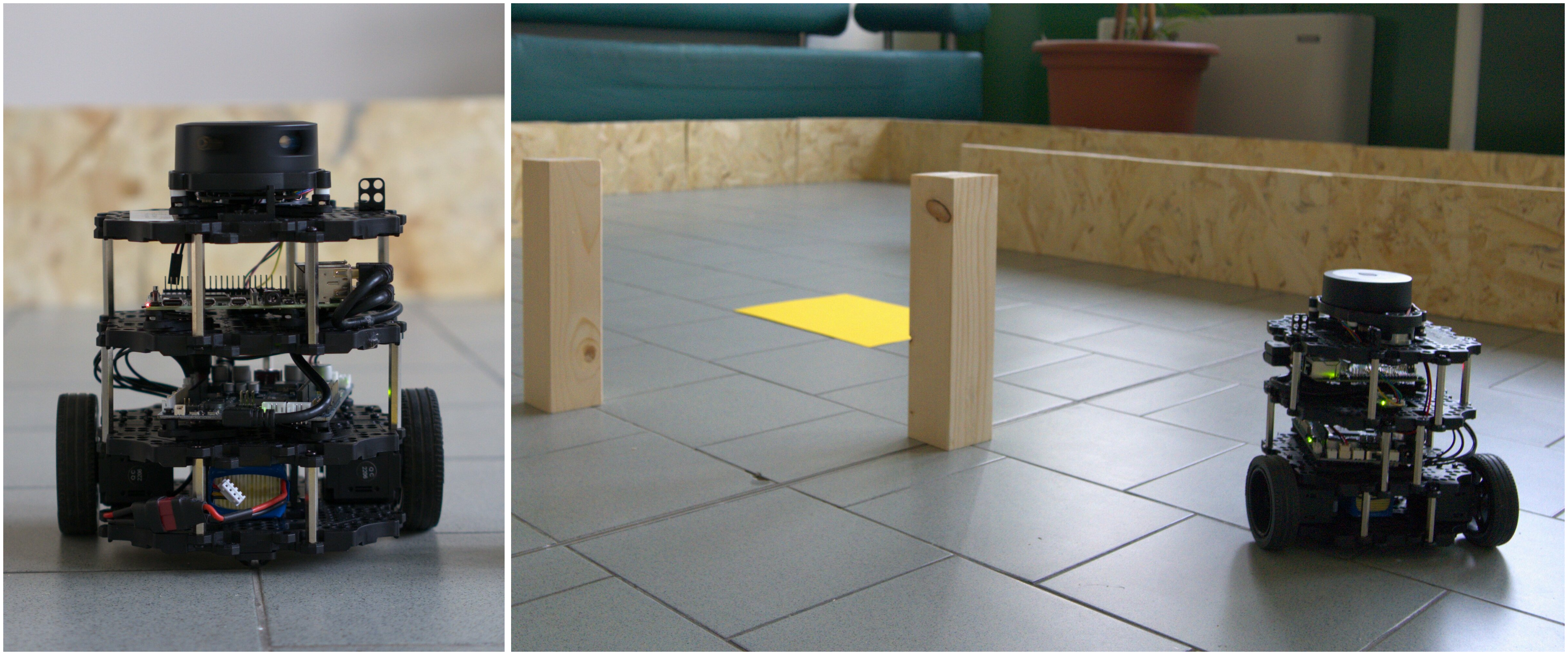
Figure 2: The Robotis Turtlebot 3 platform, navigating in an arena. The image on the left depicts a static robot, and the image on the right depicts the robot moving towards the destination (the yellow square), while avoiding two wooden obstacles in its route.

Figure 3: An example of a simulated Turtlebot entering a 2-step loop. The white and red dashed lines represent the lidar beams (white indicates “clear”, and red indicates that an obstacle is detected). The yellow square represents the target position; and the blue arrows indicate rotation. In the first row, from left to right, the Turtlebot is stuck in an infinite loop, alternating between right and left turns. Given the deterministic nature of the system, the agent will continue to select these same actions, ad infinitum. In the second row, from left to right, we present an almost identical configuration, but with an obstacle located $30\degree$ to the robot’s left (circled in blue). The presence of the obstacle changes the input to the DNN, and allows the Turtlebot to avoid entering the infinite loop; instead, it successfully navigates to the target.

The Mapless Navigation Problem. Robotic navigation is the task of navigating a robot (in our case, the Turtlebot) through an arena. The robot’s goal is to reach a target destination while adhering to predefined restrictions; e.g., selecting as short a path as possible, avoiding obstacles, or optimizing energy consumption. In recent years, robotic navigation tasks have received a great deal of attention [82, 90], primarily due to their applicability to autonomous vehicles.

We study here the popular mapless variant of the robotic navigation problem, where the robot can rely only on local observations (i.e., its sensors), without any information about the arena’s structure or additional data from external sources. In this setting, which has been studied extensively [77], the robot has access to the relative location of the target, but does not have a complete map of the arena. This makes mapless navigation a partially observable problem, and among the most challenging tasks to solve in the robotics domain [77, 16, 92, 58].

DRL-Controlled Mapless Navigation. State-of-the-art solutions to mapless navigation suggest training a DRL policy to control the robot. Such DRL-based solutions have obtained outstanding results from a performance point of view [63]. For example, recent work by Marchesini et al. [57] has demonstrated how DRL-based agents can be applied to control the Turtlebot in a mapless navigation setting, by training a DNN with a simple architecture, including two hidden layers. Following this recent work, in our case study we used the following topology for DRL policies:

• An input layer with nine neurons. These include seven neurons representing the Turtlebot’s lidar readings. The additional, non-lidar inputs include one neuron representing the relative angle between the robot and the target, and one neuron representing the robot’s distance from the target. A scheme of the inputs appears in Fig. 4a.

• Two subsequent fully-connected layers, each consisting of $16$ neurons, and followed by a ReLU activation layer.

• An output layer with three neurons, each corresponding to a different (discrete) action that the agent can choose to execute in the following step: move FORWARD, turn LEFT, or turn RIGHT.

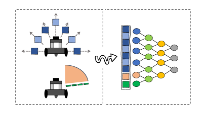
(a) The DRL controller

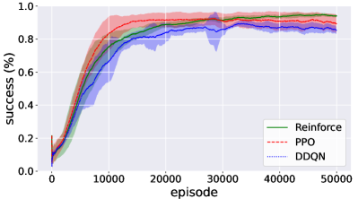
(b) Average success rates

Figure 4: (a) The DRL controller used for the robot in our case study. The DRL has nine input neurons: seven lidar sensor readings (blue), one input indicating the relative angle (orange) between the robot and the target, and one input indicating the distance (green) between the robot and the target. (b) The average success rates of models trained by each of the three DRL training algorithms, per training episode.

While the aforementioned DRL topology has been shown to be efficient for robotic navigation tasks, finding the optimal training algorithm and reward function is still an open problem. As part of our work, we trained multiple deterministic policies using the DRL algorithms presented in Section 2: DDQN [79], Reinforce [89], and PPO [68]. For the reward function, we used the following formulation:

$$\mathbb{R}_{t}=(d_{t-1}-d_{t})\cdot\alpha-\beta,$$

where $d_{t}$ is the distance from the target at time-step $t$; $\alpha$ is a normalization factor used to guarantee the stability of the gradient; and $\beta$ is a fixed value, decreased at each time-step, and resulting in a total penalty proportional to the length of the path (by minimizing this penalty, the agent is encouraged to reach the target quickly). In our evaluation, we empirically selected $\alpha=3$ and $\beta=0.001$. Additionally, we added a final reward of $+1$ when the robot reached the target, or $-1$ in case it collided with an obstacle. For additional information regarding the parameters chosen for the training phase, see Section A of the Appendix.

DRL Training and Results. Using the training algorithms mentioned in Section 2, we trained a collection of DRL agents to solve the Turtlebot mapless navigation problem. We ran a stochastic training process, and thus obtained varied agents; of these, we only kept those that achieved a success rate of at least $96\%$ during training. A total of $780$ models were selected, consisting of $260$ models per each of the three training algorithms. More specifically, for each algorithm, all $260$ models were generated from $52$ random seeds. Each seed gave rise to a family of $5$ models, where the individual family members differ in the number of training episodes used for training them. Fig. 4b shows the trained models’ average success rate, for each algorithm used. We note that PPO was generally the fastest to achieve high accuracy. However, all three training algorithms successfully produced highly accurate agents.

4 Using Verification for Model Selection

All of our trained models achieved very high success rates, and so, at face value, there was no reason to favor one over the other. However, as we show next, a verification-based approach can expose multiple subtle differences between them. As our evaluation criteria, we define two properties of interest that are derived from the main goals of the robotic controller: (i) reaching the target; and (ii) avoiding collision with obstacles. Employing verification, we use these criteria to identify models that may fail to fulfill their goals, e.g., because they collide with various obstacles, are overly conservative, or may enter infinite loops without reaching the target. We now define the properties that we used, and the results of their verification are discussed in Section 5. Additional details regarding the precise encoding of our queries appear in Section D of the Appendix.

Collision Avoidance. Collision avoidance is a fundamental and ubiquitous safety property [17] for navigation agents. In the context of Turtlebot, our goal is to check whether there exists a setting in which the robot is facing an obstacle, and chooses to move forward — even though it has at least one other viable option, in the form of a direction in which it is not blocked. In such situations, it is clearly preferable to choose to turn LEFT or RIGHT instead of choosing to move FORWARD and collide. See Fig. 5 for an illustration.

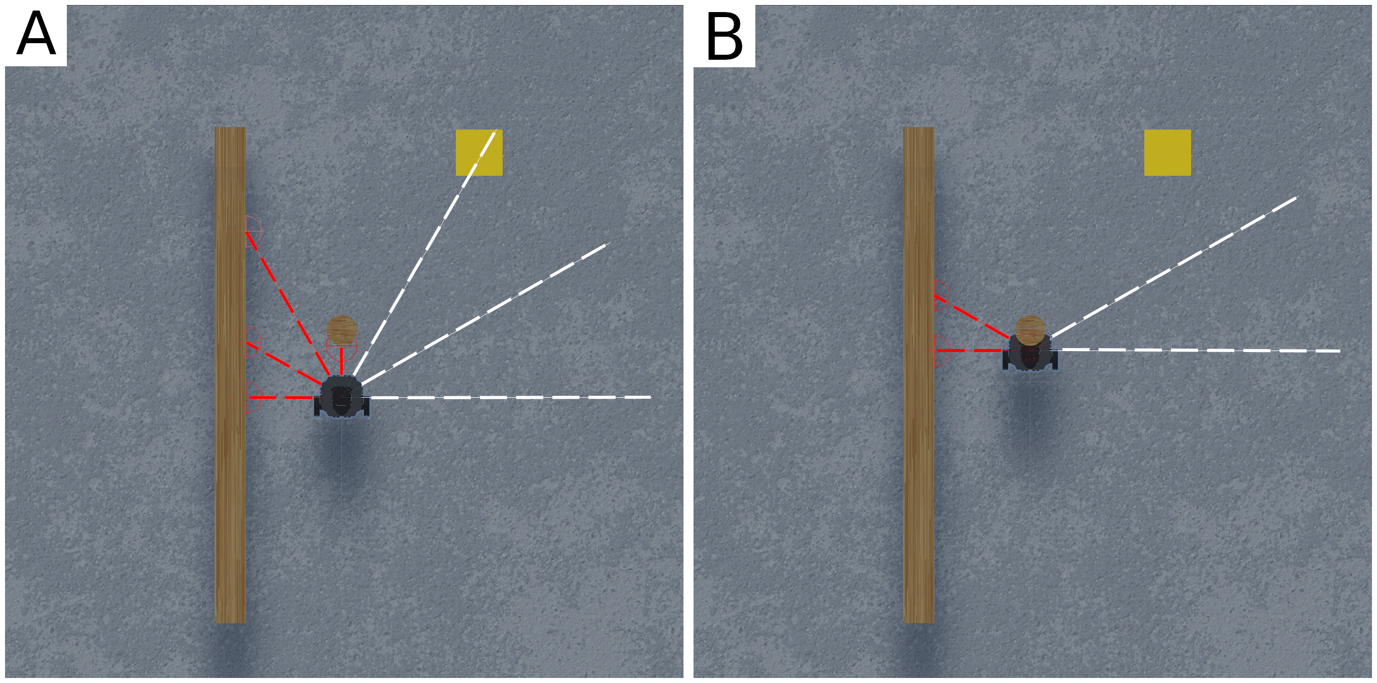
Figure 5: Example of a single-step collision. The robot is not blocked on its right and can avoid the obstacle by turning (panel A), but it still chooses to move forward — and collides (panel B).

Given that turning LEFT or RIGHT produces an in-place rotation (i.e., the robot does not change its position), the only action that can cause a collision is FORWARD. In particular, a collision can happen when an obstacle is directly in front of the robot, or is slightly off to one side (just outside the front lidar’s field of detection). More formally, we consider the safety property “the robot does not collide at the next step”, with three different types of collisions:

• FORWARD COLLISION: the robot detects an obstacle straight ahead, but nevertheless makes a step forward and collides with the obstacle.

• LEFT COLLISION: the robot detects an obstacle ahead and slightly shifted to the left (using the lidar beam that is $30\degree$ to the left of the one pointing straight ahead), but makes a single step forward and collides with the obstacle. The shape of the robot is such that in this setting, a collision is unavoidable.

• RIGHT COLLISION: the robot detects an obstacle ahead and slightly shifted to the right, but makes a single step forward and collides with the obstacle.

Recall that in mapless navigation, all observations are local — the robot has no sense of the global map, and can encounter any possible obstacle configuration (i.e., any possible sensor reading). Thus, in encoding these properties, we considered a single invocation of the DRL agent’s DNN, with the following constraints:

1. All the sensors that are not in the direction of the obstacle receive a lidar input indicating that the robot can move either LEFT or RIGHT without risk of collision. This is encoded by lower-bounding these inputs.

2. The single input in the direction of the obstacle is upper-bounded by a value matching the representation of an obstacle, close enough to the robot so that it will collide if it makes a move FORWARD.

3. The input representing the distance to the target is lower-bounded, indicating that the target has not yet been reached (encouraging the agent to make a move).

The exact encoding of these properties is based on the physical characteristics of the robot and the lidar sensors, as explained in Section B of the Appendix.

Infinite Loops. Whereas collision avoidance is the natural safety property to verify in mapless navigation controllers, checking that progress is eventually made towards the target is the natural liveness property. Unfortunately, this property is difficult to formulate due to the absence of a complete map. Instead, we settle for a weaker property, and focus on verifying that the robot does not enter infinite loops (which would prevent it from ever reaching the target).

Unlike the case of collision avoidance, where a single step of the DRL agent could constitute a violation, here we need to reason about multiple consecutive invocations of the DRL controller, in order to identify infinite loops. This, again, is difficult to encode due to the absence of a global map, and so we focus on in-place loops: infinite sequences of steps in which the robot turns LEFT and RIGHT, but without ever moving FORWARD, thus maintaining its current location ad infinitum.

Our queries for identifying in-place loops encode that: (i) the robot does not reach the target in the first step; (ii) in the following $k$ steps, the robot never moves FORWARD, i.e., it only performs turns; and (iii) the robot returns to an already-visited configuration, guaranteeing that the same behavior will be repeated by our deterministic agents. The various queries differ in the choice of $k$, as well as in the sequence of turns performed by the robot. Specifically, we encode queries for identifying the following kinds of loops:

• ALTERNATING LOOP: a loop where the robot performs an infinite sequence of $\langle\texttt{LEFT},\texttt{RIGHT},\texttt{LEFT},\texttt{RIGHT},\texttt{LEFT}...\rangle$ moves. A query for identifying this loop encodes $k=2$ consecutive invocations of the DRL agent, after which the robot’s sensors will again report the exact same reading, leading to an infinite loop. An example appears in Fig. 3. The encoding uses the “sliding window” principle, on which we elaborate later.

• LEFT CYCLE, RIGHT CYCLE: loops in which the robot performs an infinite sequence of $\langle\texttt{LEFT},\texttt{LEFT},\texttt{LEFT},\ldots\rangle$ or $\langle\texttt{RIGHT},\texttt{RIGHT},\texttt{RIGHT},\ldots\rangle$ operations accordingly. Because the Turtlebot turns at a $30\degree$ angle, this loop is encoded as a sequence of $k=360\degree/30\degree=12$ consecutive invocations of the DRL agent’s DNN, all of which produce the same turning action (either LEFT or RIGHT). Using the sliding window principle guarantees that the robot returns to the same exact configuration after performing this loop, indicating that it will never perform any other action.

We also note that all the loop-identification queries include a condition for ensuring that the robot is not blocked from all directions. Consequently, any loops that are discovered demonstrate a clearly suboptimal behavior.

Specific Behavior Profiles. In our experiments, we noticed that the safe policies, i.e., the ones that do not cause the robot to collide, displayed a wide spectrum of different behaviors when navigating to the target. These differences occurred not only between policies that were trained by different algorithms, but also between policies trained by the same reward strategy — indicating that these differences are, at least partially, due to the stochastic realization of the DRL training process.

Figure 6: Comparing paths selected by policies with different bravery levels. Path $A$ takes the Turtlebot close to the obstacle (red area), and is the shortest. Path $B$ maintains a greater distance from the obstacle (light red area), and is consequently longer. Finally, path $C$ maintains such a significant distance from the obstacle (white area) that it is unable to reach the target.

Specifically, we noticed high variability in the length of the routes selected by the DRL policy in order to reach the given target: while some policies demonstrated short, efficient, paths that passed very close to obstacles, other policies demonstrated a much more conservative behavior, by selecting longer paths, and avoiding getting close to obstacles (an example appears in Fig. 6).

Thus, we used our verification-driven approach to quantify how conservative the learned DRL agent is in the mapless navigation setting. Intuitively, a highly conservative policy will keep a significant safety margin from obstacles (possibly taking a longer route to reach its destination), whereas a “braver” and less conservative controller would risk venturing closer to obstacles. In the case of Turtlebot, the preferable DRL policies are the ones that guarantee the robot’s safety (with respect to collision avoidance), and demonstrate a high level of bravery — as these policies tend to take shorter, optimized paths (see path A in Fig. 6), which lead to reduced energy consumption over the entire trail.

Bravery assessment is performed by encoding verification queries that identify situations in which the Turtlebot can move forward, but its control policy chooses not to. Specifically, we encode single invocations of the DRL model, in which we bound the lidar inputs to indicate that the Turtlebot is sufficiently distant from any obstacle and can safely move forward. We then use the verifier to determine whether, in this setting, a FORWARD output is possible. By altering and adjusting the bounds on the central lidar sensor, we can control how far away the robot perceives the obstacle to be. If we limit this distance to large values and the policy will still not move FORWARD, it is considered conservative; otherwise, it is considered brave. By conducting a binary search over these bounds [6], we can identify the shortest distance from an obstacle for which the policy safely orders the robot to move FORWARD. This value’s inverse then serves as a bravery score for that policy.

Design-for-Verification: Sliding Windows. A significant challenge that we faced in encoding our verification properties, especially those that pertain to multiple consecutive invocations of the DRL policy, had to do with the local nature of the sensor readings that serve as input to the DNN. Specifically, if the robot is in some initial configuration that leads to a sensor input $x$, and then chooses to move forward and reaches a successor configuration in which the sensor input is $x^{\prime}$, some connection between $x$ and $x^{\prime}$ must be expressed as part of the verification query (i.e., nearby obstacles that exist in $x$ cannot suddenly vanish in $x^{\prime}$). In the absence of a global map, this is difficult to enforce.

In order to circumvent this difficulty, we used the sliding window principle, which has proven quite useful in similar settings [26, 6]. Intuitively, the idea is to focus on scenarios where the connections between $x$ and $x^{\prime}$ are particularly straightforward to encode — in fact, most of the sensor information that appeared in $x$ also appears in $x^{\prime}$. This approach allows us to encode multistep queries, and is also beneficial in terms of performance: typically, adding sliding-window constraints reduces the search space explored by the verifier, and expedites solving the query.

In the Turtlebot setting, this is achieved by selecting a robot configuration in which the angle between two neighboring lidar sensors is identical to the turning angle of the robot (in our case, $30\degree$). This guarantees, for example, that if the central lidar sensor observes an obstacle at distance $d$ and the robot chooses to turn RIGHT, then at the next step, the lidar sensor just to the left of the central sensor must detect the same obstacle, at the same distance $d$. More generally, if at time-step $t$ the 7 lidar readings (from left to right) are $\langle l_{1},\ldots,l_{7}\rangle$ and the robot turns RIGHT, then at time-step $t+1$ the 7 readings are $\langle l_{2},l_{3},\ldots,l_{7},l_{8}\rangle$, where only $l_{8}$ is a new reading. The case for a LEFT turn is symmetrical. By placing these constraints on consecutive states encountered by the robot, we were able to encode complex properties that involve multiple time-steps, e.g., as in the aforementioned infinite loops. An illustration appears in Fig. 3.

5 Experimental Evaluation

Next, we ran verification queries with the aforementioned properties, in order to assess the quality of our trained DRL policies. The results are reported below. In many cases, we discovered configurations in which the policies would cause the robot to collide or enter infinite loops; and we later validated the correctness of these results using a physical robot. We strongly encourage the reader to watch a short video clip that demonstrates some of these results [4]. Our code and benchmarks are also available online [3]. In our experiments, We used the Marabou verification engine [45] as our backend, although other engines could be used as well. For additional details regarding the experiments, we refer the reader to Section D of the Appendix.

Model Selection. In this set of experiments, we used verification to assess our trained models. Specifically, we used each of the three training algorithms (DDQN, Reinforce, PPO) to train $260$ models, creating a total of $780$ models. For each of these, we verified six properties of interest: three collision properties (FORWARD COLLISION, LEFT COLLISION, RIGHT COLLISION), and three loop properties (ALTERNATING LOOP, LEFT CYCLE, RIGHT CYCLE), as described in Section 4. This gives a total of $4680$ verification queries. We ran all queries with a TIMEOUT value of $12$ hours and a MEMOUT limit of $2G$; the results are summarized in Table 1. The single-step collision queries usually terminated within seconds, and the $2$-step queries encoding an ALTERNATING LOOP usually terminated within minutes. The $12$-step cycle queries, which are more complex, usually ran for a few hours. $9.6\%$ of all queries hit the TIMEOUT limit (all from the $12$-step cycle category), and none of the queries hit the MEMOUT limit.

	LEFT COLLISION		FORWARD COLLISION		RIGHT COLLISION
Algorithm	SAT	UNSAT	SAT	UNSAT	SAT	UNSAT
DDQN	259	1	248	12	258	2
Reinforce	255	5	254	6	252	8
PPO	196	64	197	63	207	53

	ALTERNATING LOOP		LEFT CYCLE		RIGHT CYCLE		INSTABILITY
Algorithm	SAT	UNSAT	SAT	UNSAT	SAT	UNSAT	# alternations
DDQN	260	0	56	77	56	61	21
Reinforce	145	115	5	185	120	97	10
PPO	214	45	26	198	30	198	1

Table 1: Results of the policy verification queries. We verified six properties over each of the $260$ models trained per algorithm; SAT indicates that the property was violated, whereas UNSAT indicates that it held (to reduce clutter, we omit TIMEOUT and FAIL results). The rightmost column reports the stability values of the various training methods. For the full results see [3].

Our results exposed various differences between the trained models. Specifically, of the $780$ models checked, $752$ (over $96\%$) violated at least one of the single-step collision properties. These $752$ collision-prone models include all $260$ DDQN-trained models, $256$ Reinforce models, and $236$ PPO models. Furthermore, when we conducted a model filtering process based on all six properties (three collisions and three infinite loops), we discovered that $778$ models out of the total of $780$ (over $99.7\%$!) violated at least one property. The only two models that passed our filtering process were trained by the PPO algorithm.

Further analyzing the results, we observed that PPO models tended to be safer to use than those trained by other algorithms: they usually had the fewest violations per property. However, there are cases in which PPO proved less successful. For example, our results indicate that PPO-trained models are more prone to enter an ALTERNATING LOOP than those trained by Reinforce. Specifically, $214$ ($82.3\%$) of the PPO models have entered this undesired state, compared to $145$ ($55.8\%$) of the Reinforce models. We also point out that, similarly to the case with collision properties, all DDQN models violated this property.

Finally, when considering $12$-step cycles (either LEFT CYCLE or RIGHT CYCLE), $44.8\%$ of the DDQN models entered such cycles, compared to $30.7\%$ of the Reinforce models, and just $12.4\%$ of the PPO models. In computing these results, we computed the fraction of violations (SAT queries) out of the number of queries that did not time out or fail, and aggregated SAT results for both cycle directions.

Interestingly, in some cases, we observed a bias toward violating a certain subcase of various properties. For example, in the case of entering full cycles — although $125$ (out of $520$) queries indicated that Reinforce-trained agents may enter a cycle in either direction, in $96\%$ of these violations, the agent entered a RIGHT CYCLE. This bias is not present in models trained by the other algorithms, where the violations are roughly evenly divided between cycles in both directions.

We find that our results demonstrate that different “black-box” algorithms generalize very differently with respect to various properties. In our setting, PPO produces the safest models, while DDQN tends to produce models with a higher number of violations. We note that this does not necessarily indicate that PPO-trained models perform better, but rather that they are more robust to corner cases. Using our filtering mechanism, it is possible to select the safest models among the available, seemingly equivalent candidates.

Next, we used verification to compute the bravery score of the various models. Using a binary search, we computed for each model the minimal distance a dead-ahead obstacle needs to have for the robot to safely move forward. The search range was $[0.18,1]$ meters, and the optimal values were computed up to a $0.01$ precision (see Section D of the Appendix for additional details). Almost all binary searches terminated within minutes, and none hit the TIMEOUT threshold.

By first filtering the models based on their safe behavior, and then by their bravery scores, we are able to find the few models that are both safe (do not collide), and not overly conservative. These models tend to take efficient paths, and may come close to an obstacle, but without colliding with it. We also point out that over-conservativeness may significantly reduce the success rate in specific scenarios, such as cases in which the obstacle is close to the target. Specifically, of the only two models that survived the first filtering stage, one is considerably more conservative than the other — requiring the obstacle to be twice as distant as the other, braver, model requires it to be, before moving forward.

Algorithm Stability Analysis. As part of our experiments, we used our method to assess the three training algorithms — DDQN, PPO, and Reinforce. Recall that we used each algorithm to train $52$ families of $5$ models each, in which the models from the same family are generated from the same random seed, but with a different number of training iterations. While all models obtained a high success rate, we wanted to check how often it occurred that a model successfully learned to satisfy a desirable property after some training iterations, only to forget it after additional iterations. Specifically, we focused on the $12$-step full-cycle properties (LEFT CYCLE and RIGHT CYCLE), and for each family of $5$ models checked whether some models satisfied the property while others did not.

We define a family of models to be unstable in the case where a property holds in the family, but ceases to hold for another model from the same family with a higher number of training iterations. Intuitively, this means that the model “forgot” a desirable property as training progressed. The instability value of each algorithm type is defined to be the number of unstable 5-member families.

Although all three algorithms produced highly accurate models, they displayed significant differences in the stability of their produced policies, as can be seen in the rightmost column of Table 1. Recall that we trained $52$ families of models using each algorithm, and then tested their stability with respect to two properties (corresponding to the two full cycle types). Of these, the DDQN models display $21$ unstable alternations — more than twice the number of alterations demonstrated by Reinforce models ($10$), and significantly higher than the number of alternations observed among the PPO models ($1$).

These results shed light on the nature of these training algorithms — indicating that DDQN is a significantly less stable training algorithm, compared to PPO and Reinforce. This is in line with previous observations in non-verification-related research [68], and is not surprising, as the primary objective of PPO is to limit the changes the optimizer performs between consecutive training iterations.

Gradient-Based Methods. We also conducted a thorough comparison between our verification-based approach and competing gradient-based methods. Although gradient-based attacks are extremely scalable, our results (summarized in Table 2 of the Appendix) show that they may miss many of the violations found by our complete, verification-based procedure. For example, when searching for collisions, our approach discovered a total of $2126$ SAT results, while the gradient-based method discovered only $1421$ SAT results — a $33\%$ decrease (!). In addition, given that gradient-based methods are unable to return UNSAT, they are also incapable of proving that a property always holds, and hence cannot formally guarantee the safety of a policy in question. Thus, performing model selection based on gradient-based methods could lead to skewed results. We refer the reader to Section E of the Appendix, in which we elaborate on gradient attacks and the experiments we ran, demonstrating the advantages of our approach for model selection, when compared to gradient-based methods.

6 Related Work

Due to the increasing popularity of DNNs, the formal methods community has put forward a plethora of tools and approaches for verifying DNN correctness [24, 43, 44, 45, 37, 48, 35, 70, 30, 78, 53]. Recently, the verification of systems involving multiple DNN invocations, as well as hybrid systems with DNN components, has been receiving significant attention [28, 80, 11, 46, 6, 21, 22, 73]. Our work here is another step toward applying DNN verification techniques to additional, real-world systems and properties of interest.

In the robotics domain, multiple approaches exist for increasing the reliability of learning-based systems [65, 91, 81]; however, these methods are mostly heuristic in nature [29, 1, 56]. To date, existing techniques rely mostly on Lagrangian multipliers [71, 67, 52], and do not provide formal safety guarantees; rather, they optimize the training in an attempt to learn the required policies [14]. Other, more formal approaches focus solely on the systems’ input-output relations [55, 18], without considering multiple invocations of the agent and its interactions with the environment. Thus, existing methods are not able to provide rigorous guarantees regarding the correctness of multistep robotic systems, and do not take into account sequential decision making — which renders them insufficient for detecting various safety and liveness violations.

Our approach is orthogonal and complementary to many existing safe DRL techniques. Reward reshaping and shielding techniques (e.g., [2]) improve safety by altering the training loop, but typically afford no formal guarantees. Our approach can be used to complement them, by selecting the most suitable policy from a pool of candidates, post-training. Guard rules and runtime shields are beneficial for preventing undesirable behavior of a DNN agent, but are sometimes less suited for specifying the desired actions it should take instead. In contrast, our approach allows selecting the optimal policy from a pool of candidates, without altering its decision-making.

7 Conclusion

Through the case study described in this paper, we demonstrate that current verification technology is applicable to real-world systems. We show this by applying verification techniques for improving the navigation of DRL-based robotic systems. We demonstrate how off-the-shelf verification engines can be used to conduct effective model selection, as well as gain insights into the stability of state-of-the-art training algorithms. As far as we are aware, ours is the first work to demonstrate the use of formal verification techniques on multistep properties of actual, real-world robotic navigation platforms. We also believe the techniques developed here will allow the use of verification to improve additional multistep systems (autonomous vehicles, surgery-aiding robots, etc.), in which we can impose a transition function between subsequent steps. However, our approach is limited by DNN-verification technology, which we use as a black-box backend. As that technology becomes more scalable, so will our approach. Moving forward, we plan to generalize our work to richer environments — such as cases where a memory-enhanced agent interacts with moving objects, or even with multiple agents in the same arena, as well as running additional experiments with deeper networks, and more complex DRL systems. In addition, we see probabilistic verification of stochastic policies as interesting future work.

Acknowledgements. The work of Amir, Yerushalmi and Katz was partially supported by the Israel Science Foundation (grant number 683/18). The work of Amir was supported by a scholarship from the Clore Israel Foundation. The work of Corsi, Marzari, and Farinelli was partially supported by the “Dipartimenti di Eccellenza 2018-2022” project, funded by the Italian Ministry of Education, Universities, and Research (MIUR). The work of Yerushalmi and Harel was partially supported by a research grant from the Estate of Harry Levine, the Estate of Avraham Rothstein, Brenda Gruss and Daniel Hirsch, the One8 Foundation, Rina Mayer, Maurice Levy, and the Estate of Bernice Bernath, grant 3698/21 from the ISF-NSFC (joint to the Israel Science Foundation and the National Science Foundation of China), and a grant from the Minerva foundation. We thank Idan Refaeli for his contribution to this project.

Appendices

Appendix A Training the DRL Models

In this Appendix, we elaborate on the hyperparameters used for training, alongside various implementation details. The code is based on the BasicRL baselines. Our full code for training, as well as our original models, can be found in our publicly-available artifact accompanying this paper [3].

General Parameters

• episode limit: 100,000

• number of hidden layers: 2

• size of hidden layers: 16

• gamma ($\gamma$): 0.99

To facilitate our experiments, we followed [57] — and used the same network topology, i.e., two fully-connected ReLU layers, but focused on the smallest layer size that still achieved state-of-the-art results: $16$ neurons, instead of $64$ in [57], as these achieved similar accuracy and allowed us to expedite verification.

An additional difference, between our setting and the one appearing in [57], is that our agents have three outputs, instead of five. However, this is beneficial, as our agents achieve similar rewards to those reported in [57], and are more straightforward to verify (“design-for-verification”).

DDQN Parameters

For the DDQN experiments, we rely on the Double DQN implementation (DDQN) with a “soft” update performed at each step. The network is a standard feed-forward DNN, without dueling architecture.

• memory limit: 5,000

• epochs: 40

• batch size: 128

• $\epsilon$-decay: 0.99995

• tau ($\tau$): 0.005

Reinforce Parameters

Our implementation is based on a version of Reinforce which directly implements the policy gradient theorem [75]. The strategy for the update rule is a pure Monte Carlo approach, without temporal difference rollouts.

• memory limit: None

• trajectory update frequency: 20

• trajectory reduction strategy: sum

PPO Parameters

For the value function estimation and the critic update, we adopted a 1-step temporal difference strategy (TD-1). The update rule follows the guidelines of the OpenAI’s Spinning Up documentation.

• memory limit: None

• trajectory update frequency: 20

• trajectory reduction strategy: sum

• critic batch size: 128

• critic epochs: 60

• critic network size: same as actor

• PPO clip: 0.2

Random Seeds for Reproducibility

We now present a complete list of our seeds, sorted by value:

[$35$, $47$, $67$, $68$, $73$, $76$, $77$, $81$, $90$, $91$, $114$, $128$, $158$, $165$, $174$, $176$, $180$, $196$, $201$, $215$, $234$, $239$, $240$, $267$, $286$, $296$, $298$, $299$, $303$, $308$, $318$, $319$, $321$, $343$, $352$, $379$, $381$, $393$, $399$, $418$, $425$, $444$, $457$, $491$, $502$, $512$, $518$, $528$, $530$, $535$, $540$, $549$]

At each execution, we fed the same seeds to procedures from the Random, NumPy and TensorFlow Python modules.

Appendix B Technical Specifications of the Robot

In this Appendix, we describe the details regarding the technical specifications of the robot, its sensors, and our design choices. We performed our experiments on the Robotis Turtlebot 3, in the burger version. Turtlebot is a small research and development platform ($138$mm x $178$mm x $192$mm), that includes a set of various sensors for mapping and navigation:

• $360\degree$ lidar sensor (with a maximal distance of $3.5$ m)

• Raspberry Pi 3 to control the platform

• Gyroscope, Accelerometer, and Magnetometer sensors

• (optional) Raspberry Pi Camera for perception

The manufacturer provides all the libraries and scripts for full compatibility with the standard Robotic Operating System (ROS). The robot is designed to receive continuous input (linear and angular velocity). In our settings, we discretized the action space: therefore a single step FORWARD corresponds to a linear translation of $5$ cm, while a LEFT/RIGHT turn produces a rotation of $30\degree$ in the desired direction.

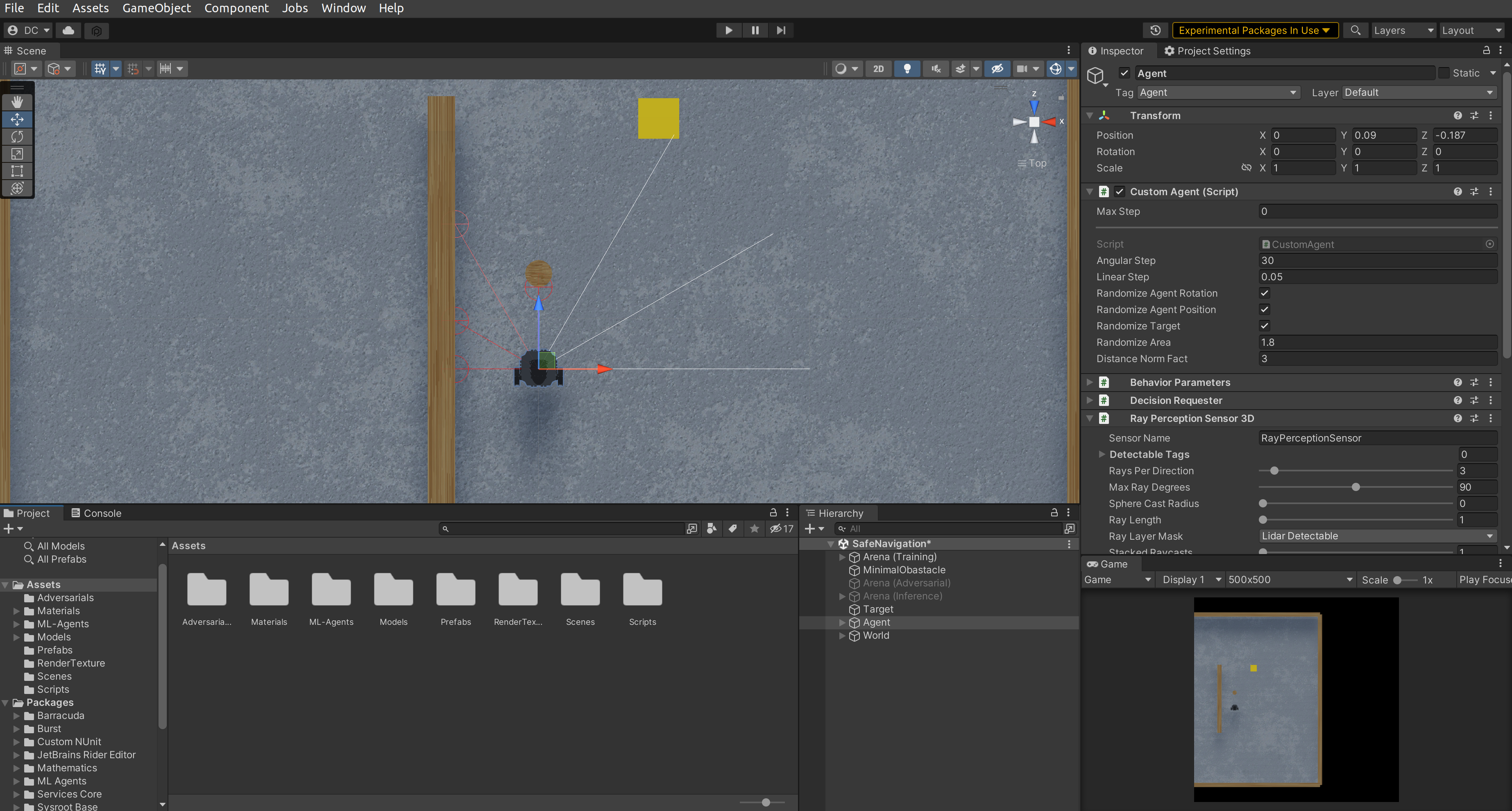
Figure 7: The Unity3D engine with our simulation environment.

To perform the training of our robot, we rely on Unity3D, a popular engine originally designed for game development, that has recently been adopted for robotics simulation [64, 55]. In particular, the built-in physics engine, the powerful $3D$ rendering algorithm and the time control system (which allows speeding up the simulation by more than $10$ times), have made Unity3D a very powerful tool in these contexts [42]. Fig. 7 depicts an example of our Turtlebot3 environment in the Unity3D simulator. A key advantage of mapless navigation is that the robot can access only local observations. Thus, the robot can “see” only the distance to the nearest collision point; hence the agent’s decisions are agnostic to the actual shape and size of the obstacles, and thus our system is encouraged to generalize to unseen environments during training.

Appendix C Adversarial Trajectories

In this Appendix, we depict a complete trajectory of a RIGHT CYCLE, as seen in Fig. 8. We note that in this, and other, infinite-loop trajectories, it is crucial to encode that the first and last states of the trajectory are identical (e.g., Subfig. $A$ and Subfig. $L$ in Fig. 8). Thus, given the deterministic nature of the controller, the robot will repeat the same sequence of actions, ending in an infinite loop, in which it constantly turns RIGHT.

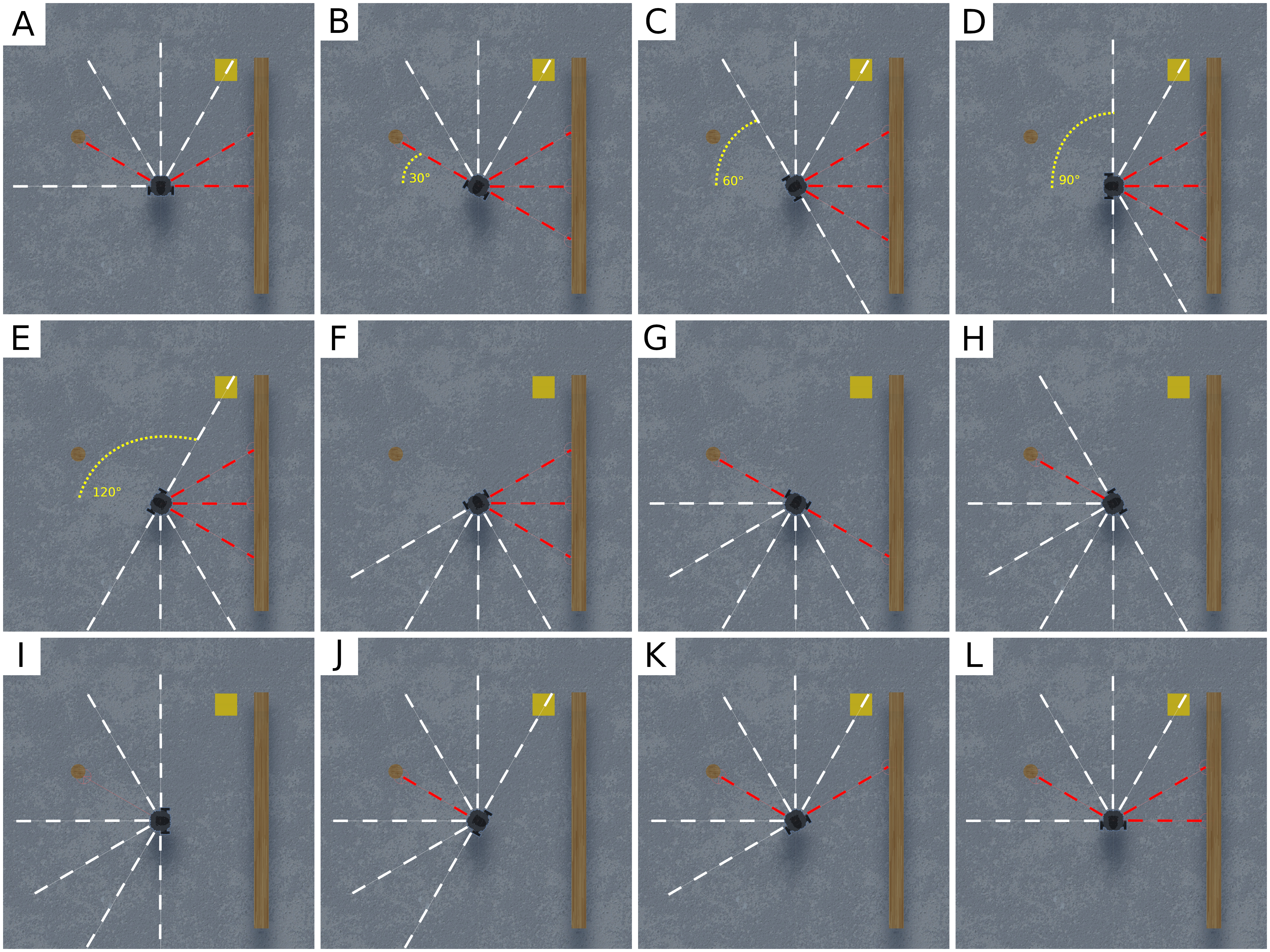
Figure 8: A 12-step trajectory of an infinite RIGHT CYCLE. The white and red dashed lines represent the lidar scan (white indicates a clear path; red indicates an obstacle is present), while the yellow square represents the target position towards which the robot navigates. The yellow dotted line represents the angular step the robot performs in the first six steps. Given that the spacing between each lidar scan is the same as the angular step size ($30\degree$), at each time-step it is possible to encode the sliding window for the state. The trajectory of a LEFT CYCLE is symmetric.

Appendix D Encoding Verification Queries

In this Appendix, we formally define the complete list of properties we analyzed in our experiments. All values are calibrated based on the technical specifications of the robot, and the size of the discrete actions presented in this paper.

Notice that, the symbol $x_{n}^{t}$ corresponds to the input node $n$ of the network at time $t$, while $y_{n}^{t}$ is the output node $n$ at time $t$. Time ($t$) is omitted for the one-step properties (i.e., $k$=$1$).

Determinsitic Policies and Stochastic Policies. In order to compare DDQN to the stochastic policies (Reinforce and PPO), we first trained the stochastic policies as usual, and then treated them as deterministic. We note that in the case of stochastic policies, our approach can only detect whether a property may be violated, and not how likely the violation is.

Marabou. All our queries were dispatched using the sound and complete Marabou verification engine [45, 84]. Marabou is a modern DNN verifier, whose core consists of a native Simplex solver, combined with abstraction and abstract-interpretation techniques [83, 70, 25, 62], splitting heuristics [85], optimization capabilities [72], and enhanced to support varied activation functions [7] and recurrent networks [40]. Marabou has been previously applied to various verification-based tasks, such as network repair [66, 32], network simplification [50, 31], ensemble selection [8], and more [5, 15, 19, 38, 87]. The Marabou engine supports DNNs with ReLU layers, max-pooling, convolution, absolute value, and sign layers; and also supports sigmoids and softmax constraints.

D.1 Property Constraints

Trivial Bounds: all the inputs of the network are normalized in the range $[0,1]$. However, in the following cases, the actual bounds can be tightened: (i) the true lower-bound for a lidar scan is $0.135$, given that the lidar scan is positioned in the center of the robot, therefore the size of the robot itself constitutes a minimal distance from an obstacle; (ii) this lower bound can be further tightened to a value of $0.2$ to guarantee enough space for all the possible actions (i.e., FORWARD, LEFT, RIGHT); (iii) for the collision properties, we found that $0.185$ is the minimal distance with which the robot can make an action FORWARD, while avoiding a collision due to a rotation; and (iv) to avoid configurations in which reaching the target position is a trivial problem (e.g., a 1-step trajectory), we set a minimum distance from the target of $0.2$.

A complete list of constraints, per property

Notice that all the properties are encoded as a negation of the expected behavior (see Sec. 4 for details). Therefore a SAT assignment corresponds to a violation of the required property. We note that the outputs $<y_{0},y_{1},y_{2}>$ correspond to the actions $<\texttt{FORWARD},\texttt{LEFT},\texttt{RIGHT}>$.

• FORWARD COLLISION ($k$=$1$): if the robot is closer than $185$ mm to an obstacle in front, never select the action FORWARD. If violated, the robot collides in, at most, two steps.

  • Precondition (P): $x_{i}\in[0.2,1]\text{ for }i=[0,1,2,4,5,6]\land x_{3}\in[0.135,0.185]\land x_{7}\in[0,1]\land x_{8}\in[0.2,1]$

  • Postcondition (Q): $y_{0}>y_{1}$ $\land$ $y_{0}>y_{2}$

• LEFT COLLISION ($k$=$1$): if the robot is closer than $185$ mm to an obstacle on the front-left, never select the action FORWARD. If violated, the robot collides in, at most, two steps.

  • Precondition (P): $x_{i}\in[0.2,1]\text{ for }i=[0,1,3,4,5,6]\land x_{2}\in[0.135,0.185]\land x_{7}\in[0,1]\land x_{8}\in[0.2,1]$

  • Postcondition (Q): $y_{0}>y_{1}$ $\land$ $y_{0}>y_{2}$

• RIGHT COLLISION ($k$=$1$): if the robot is closer than $185$ mm to an obstacle on the front-right, never select the action FORWARD. If violated, the robot will collide in, at most, two steps.

  • Precondition (P): $x_{i}\in[0.2,1]\text{ for }i=[0,1,2,3,5,6]\land x_{4}\in[0.135,0.185]\land x_{7}\in[0,1]\land x_{8}\in[0.2,1]$

  • Postcondition (Q): $y_{0}>y_{1}$ $\land$ $y_{0}>y_{2}$

• ALTERNATING LOOP ($k$=$2$): for all possible positions of the target and the obstacles, never sequentially select the actions RIGHT and then immediately LEFT. If violated, the robot gets stuck in an infinite 2-step loop.

  • Precondition (P): $x_{i}^{t}\in[0.2,1]\text{ for }i=[0,1,2,3,4,5,6,8]\land x_{7}^{t}\in[0,1]\land x_{i}^{t+1}\in[0.2,1]\text{ for }i=[0,1,2,3,4,5,6,8]\land x_{7}^{t+1}\in[0,1]\land x_{8}^{t}=x_{8}^{t+1}$ $\land$ $x_{i}^{t}=x_{i+1}^{t}\text{ for }i=[0,1,2,3,4,5]$ $\land$ $x_{7}^{t+1}=x_{7}^{t}\pm\frac{1}{12}$

  • Postcondition (Q): ($y_{2}^{t}>y_{0}^{t}$ $\land$ $y_{2}^{t}>y_{1}^{t}$) $\land$ ($y_{1}^{t+1}>y_{0}^{t+1}$ $\land$ $y_{1}^{t+1}>y_{2}^{t+1}$)

  Given the symmetric nature of this property, the same encoding allowed us to check both the LEFT/RIGHT and RIGHT/LEFT alternating loops. However, we note that our encodings (arbitrarily) search for trajectories starting with a turn to the RIGHT.

• LEFT CYCLE and RIGHT CYCLE ($k$=$12$): for all possible positions of the target and the obstacles, if the robot has at least one escape direction, never select in $12$ consecutive steps the action LEFT (or RIGHT). If this property is violated, the robot will get stuck in an infinite loop of $360\degree$ rotating counter-clockwise (or clockwise).

  • Precondition - bounds (P): $x_{i}^{t}\in[0.2,1]\text{ for }i=[0,1,2,3,4,5,6,8]\text{ and }t=[0,...,11]\land x_{7}^{t}\in[0,1]\text{ for }t=[0,...,11]\land x_{8}^{t}=x_{8}^{t+1}\text{ for }t=[0,...,10]$

  • Precondition - sliding window (P): to better explain the property, we refer to Fig. 9 (for RIGHT CYCLE the figure should be read from top to bottom; the opposite for LEFT CYCLE), which includes a scheme of the sliding window encoding, as explained in Sec. 4. We note that sensors (in different time-steps) are colored the same to represent that they encode the same equality constraint (e.g., $\langle L_{1},T_{0}\rangle=\langle L_{0},T_{1}\rangle$). The input relative to the distance from the target (i.e., $x_{8}^{t}$) must be the same for all the $12$ steps, while the angle (i.e., $x_{7}^{t}$) must respect the property $x_{7}^{t+1}=x_{7}^{t}\pm\frac{1}{12}$ (depending on whether RIGHT CYCLE or LEFT CYCLE is encoded).

  • Postcondition (Q): choose the same action (LEFT or RIGHT) for 12 consecutive steps.

Figure 9: A visual scheme of the “sliding window” constraints for encoding a 12-step full cycle. In the case of encoding a RIGHT CYCLE, the constraints should be read from top to bottom. In the case of encoding a LEFT CYCLE, the constraints should be read from bottom to top.

Note. The fact that the agent may enter infinite loops is not due to the turning angle matching the angle between consecutive lidar sensors; the same can happen when different angles are used, as in [57]. Configuring the lidar angles to match the turning angle is part of our methodology for facilitating verification (“sliding window”, for reducing the state space), but it does not cause the infinite loop, or any other property violation.

D.2 The Slack Margin

When searching for adversarial inputs with formal verification techniques, it is common practice to search for strong violations, i.e., requiring a minimal difference between the original output and the output generated by the adversarial input. Formally, if the original output is $y$, we consider a violation only if $y^{\prime}>y+\gamma$, for some predefined margin (“slack”) $\gamma>0$, and an output $y^{\prime}$.

In our experiments, to conduct a fair comparison between models trained by different algorithms (all outputting values in different ranges) we analyzed the empirical distribution of a random variable that consists of the difference between the “winner” (classified) output and the “runner-up” (second highest) output.

As can be seen in Fig. 10, the empirical distribution for this random variable is different (both in the shape, and values) per each of the training algorithms.

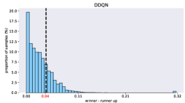
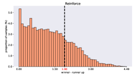
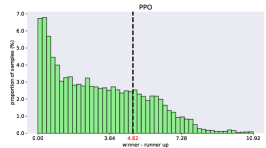
Figure 10: The empirical distribution of the difference between the “winning” (highest) output and the second-highest output. Each distribution is based on approximately $4000$ samples, taken from $N=100$ episodes for each algorithm.

Given these results, to guarantee a fair comparison between the algorithms, we used a slack variable with a value corresponding to the 75-th percentile, i.e., a value that is larger than $75\%$ of the samples. The values matching this percentile (per each training algorithm) are:

• DDQN: $0.042$

• Reinforce: $1.904$

• PPO: $4.821$

These values were chosen to be the $\gamma$ slack values encoded for the single-step ($k=1$) verification queries, i.e., queries encoding: FORWARD COLLISION, LEFT COLLISION or RIGHT COLLISION.

When encoding multistep properties (the three loop types) this slack was divided by the number of $k$ steps encoded in the relevant query. This is because each additional step adds constraints to the query and so to balance the additional constraints — the $\gamma$ slack is reduced.

For the original verification query encodings, we refer the reader to our publicly-available artifact accompanying this paper [3].

D.3 Bravery Property Results

Our verification results indicate that:

1. the braver model may move forward when the distance is slightly over $0.42$ meters; while

2. the over-conservative model never moves forward in cases where a similar obstacle is closer than $0.88$ meters.

Appendix E Comparison to Gradient-Based Methods

We also compared our verification-based method to state-of-the-art gradient attacks, which can also be used to search for property violations — and hence, in model selection. Gradient attacks are optimization methods, designed to produce inputs that are misclassified by the DNN [76]. Intuitively, starting from some arbitrary input point, these methods seek perturbations that cause significant changes to the model’s outputs — increasing the value it assigns to outputs that correspond to some (targeted) incorrect label. These perturbations are discovered using a local search that performs gradient descent on a tailored loss function [34]. It is common practice to consider a gradient-based search as successful if it finds a perturbed input on which the target label receives a score that is higher than the true label (by some predefined margin). Notice that, in contrast to complete verification methods, a gradient-based attack can only answer SAT or TIMEOUT.

In our evaluation, we ran the Basic Iterative Method (BIM) [49] — a popular gradient attack based on the Fast-Gradient Sign Method (FGSM) [34, 27]. We ran the attack on all $780$ models, searching for violations of all three single-step safety properties. Each attack ran for $40$ iterations, with a step size of $0.01$. In order to conduct a fair comparison between this gradient-based attack and our verification-based approach, we used a heuristic of choosing the initial point for the attack to be the center of the bounds for each input. In addition, we used the same slack margin by which the incorrect label should pass the correct one in all experiments, for both approaches. For additional details see Section D of the Appendix.

Algorithm	Gradient	Verification	Ratio (%)
DDQN	405	765	$53$
Reinforce	671	761	$88$
PPO	345	600	$58$
Total	$1421$	$2126$	$67$

Table 2: The number of counterexamples (SAT results) discovered using the gradient-based BIM method [49], versus our verification-based approach. The rightmost column indicates the ratio of values in the two previous columns.

Although gradient-based methods are extremely scalable, they suffer from many setbacks. Firstly, they tend to miss many violations otherwise found by verification-driven approaches (up to a third of our violations were missed, as seen in Table 2). In addition, gradient-based methods are incomplete, and thus, are unable to guarantee that some properties always hold, while sound and complete verification tools may guarantee a property holds in various settings. Another pitfall of gradient-based methods is their inadequacy to check for adversarial inputs across multiple steps (loops, in our case), bringing us to focus solely on collision properties in our comparison. Hence, although gradient approaches are ill-suited for the task described, we compared them to our approach, despite the inherent limitations of such a comparison. Still, gradient attacks are the best tool previously available, and so we believe this highlights the usefulness of our approach.

References

- [1] J. Achiam, D. Held, A. Tamar, and P. Abbeel. Constrained Policy Optimization. In Proc. 34th Int. Conf. on Machine Learning (ICML), pages 22–31, 2017.
- [2] M. Alshiekh, R. Bloem, R. Ehlers, B. Könighofer, S. Niekum, and U. Topcu. Safe Reinforcement Learning via Shielding. In Proc. 32th AAAI Conf. on Artificial Intelligence (AAAI), pages 2669–2678, 2018.
- [3] G. Amir, D. Corsi, R. Yerushalmi, L. Marzari, D. Harel, A. Farinelli, and G. Katz. Supplementary Artifact, 2022. https://zenodo.org/record/7479970.
- [4] G. Amir, D. Corsi, R. Yerushalmi, L. Marzari, D. Harel, A. Farinelli, and G. Katz. Supplementary Video, 2022. https://youtu.be/QIZqOgxLkAE.
- [5] G. Amir, Z. Freund, G. Katz, E. Mandelbaum, and I. Refaeli. veriFIRE: Verifying an Industrial, Learning-Based Wildfire Detection. In Proc. 25th Int. Symposium on Formal Methods (FM), 2023.
- [6] G. Amir, M. Schapira, and G. Katz. Towards Scalable Verification of Deep Reinforcement Learning. In Proc. 21st Int. Conf. on Formal Methods in Computer-Aided Design (FMCAD), pages 193–203, 2021.
- [7] G. Amir, H. Wu, C. Barrett, and G. Katz. An SMT-Based Approach for Verifying Binarized Neural Networks. In Proc. 27th Int. Conf. on Tools and Algorithms for the Construction and Analysis of Systems (TACAS), pages 203–222, 2021.
- [8] G. Amir, T. Zelazny, G. Katz, and M. Schapira. Verification-Aided Deep Ensemble Selection. In Proc. 22nd Int. Conf. on Formal Methods in Computer-Aided Design (FMCAD), pages 27–37, 2022.
- [9] R. Amsters and P. Slaets. Turtlebot 3 as a Robotics Education Platform. In Proc. 10th Int. Conf. on Robotics in Education (RiE), pages 170–181, 2019.
- [10] G. Avni, R. Bloem, K. Chatterjee, T. Henzinger, B. Konighofer, and S. Pranger. Run-Time Optimization for Learned Controllers through Quantitative Games. In Proc. 31st Int. Conf. on Computer Aided Verification (CAV), pages 630–649, 2019.
- [11] E. Bacci, M. Giacobbe, and D. Parker. Verifying Reinforcement Learning Up to Infinity. In Proc. 30th Int. Joint Conf. on Artificial Intelligence (IJCAI), 2021.
- [12] T. Baluta, S. Shen, S. Shinde, K. Meel, and P. Saxena. Quantitative Verification of Neural Networks and its Security Applications. In Proc. ACM SIGSAC Conf. on Computer and Communications Security (CCS), pages 1249–1264, 2019.
- [13] M. Bojarski, D. Del Testa, D. Dworakowski, B. Firner, B. Flepp, P. Goyal, L. Jackel, M. Monfort, U. Muller, J. Zhang, X. Zhang, J. Zhao, and K. Zieba. End to End Learning for Self-Driving Cars, 2016. Technical Report. http://arxiv.org/abs/1604.07316.
- [14] L. Brunke, M. Greeff, A. Hall, Z. Yuan, S. Zhou, J. Panerati, and A. Schoellig. Safe Learning in Robotics: From Learning-Based Control to Safe Reinforcement Learning. Annual Review of Control, Robotics, and Autonomous Systems, 5, 2021.
- [15] M. Casadio, E. Komendantskaya, M. Daggitt, W. Kokke, G. Katz, G. Amir, and I. Refaeli. Neural Network Robustness as a Verification Property: A Principled Case Study. In Proc. 34th Int. Conf. on Computer Aided Verification (CAV), 2022.
- [16] H. Chiang, A. Faust, M. Fiser, and A. Francis. Learning Navigation Behaviors End-to-End with AutoRL. IEEE Robotics and Automation Letters (RA-L/ICRA), 4(2):2007–2014, 2019.
- [17] E. Clarke, T. Henzinger, H. Veith, and R. Bloem. Handbook of Model Checking, volume 10. Springer, 2018.
- [18] D. Corsi, E. Marchesini, and A. Farinelli. Formal Verification of Neural Networks for Safety-Critical Tasks in Deep Reinforcement Learning. In Proc. 37th Conf. on Uncertainty in Artificial Intelligence (UAI), pages 333–343, 2021.
- [19] D. Corsi, R. Yerushalmi, G. Amir, A. Farinelli, D. Harel, and G. Katz. Constrained Reinforcement Learning for Robotics via Scenario-Based Programming, 2022. Technical Report. https://arxiv.org/abs/2206.09603.
- [20] L. Deng and Y. Liu. Deep Learning in Natural Language Processing. Springer, 2018.
- [21] S. Dutta, X. Chen, and S. Sankaranarayanan. Reachability Analysis for Neural Feedback Systems using Regressive Polynomial Rule Inference. In Proc. 22nd ACM Int. Conf. on Hybrid Systems: Computation and Control (HSCC), pages 157–168, 2019.
- [22] S. Dutta, S. Jha, S. Sankaranarayanan, and A. Tiwari. Learning and Verification of Feedback Control Systems using Feedforward Neural Networks. IFAC-PapersOnLine, 51(16):151–156, 2018.
- [23] S. Dutta, S. Jha, S. Sankaranarayanan, and A. Tiwari. Output Range Analysis for Deep Feedforward Neural Networks. In Proc. 10th NASA Formal Methods Symposium (NFM), pages 121–138, 2018.
- [24] R. Ehlers. Formal Verification of Piece-Wise Linear Feed-Forward Neural Networks. In Proc. 15th Int. Symp. on Automated Technology for Verification and Analysis (ATVA), pages 269–286, 2017.
- [25] Y. Elboher, J. Gottschlich, and G. Katz. An Abstraction-Based Framework for Neural Network Verification. In Proc. 32nd Int. Conf. on Computer Aided Verification (CAV), pages 43–65, 2020.
- [26] T. Eliyahu, Y. Kazak, G. Katz, and M. Schapira. Verifying Learning-Augmented Systems. In Proc. Conf. of the ACM Special Interest Group on Data Communication on the Applications, Technologies, Architectures, and Protocols for Computer Communication (SIGCOMM), pages 305–318, 2021.
- [27] O. Ferhat and S. Yildirim-Yayilgan. Deep Neural Network Based Malicious Network Activity Detection Under Adversarial Machine Learning Attacks. In Proc. 3rd Int. Conf. on Intelligent Technologies and Applications (INTAP), pages 280–291, 2020.
- [28] N. Fulton and A. Platzer. Safe Reinforcement Learning via Formal Methods: Toward Safe Control through Proof and Learning. In Proc. 32nd AAAI Conf. on Artificial Intelligence (AAAI), 2018.
- [29] J. Garcıa and F. Fernández. A Comprehensive Survey on Safe Reinforcement Learning. Journal of Machine Learning Research, 16(1):1437–1480, 2015.
- [30] T. Gehr, M. Mirman, D. Drachsler-Cohen, E. Tsankov, S. Chaudhuri, and M. Vechev. AI2: Safety and Robustness Certification of Neural Networks with Abstract Interpretation. In Proc. 39th IEEE Symposium on Security and Privacy (S&P), 2018.
- [31] S. Gokulanathan, A. Feldsher, A. Malca, C. Barrett, and G. Katz. Simplifying Neural Networks using Formal Verification. In Proc. 12th NASA Formal Methods Symposium (NFM), pages 85–93, 2020.
- [32] B. Goldberger, Y. Adi, J. Keshet, and G. Katz. Minimal Modifications of Deep Neural Networks using Verification. In Proc. 23rd Int. Conf. on Logic for Programming, Artificial Intelligence and Reasoning (LPAR), pages 260–278, 2020.
- [33] I. Goodfellow, Y. Bengio, and A. Courville. Deep Learning. MIT Press, 2016.
- [34] I. Goodfellow, J. Shlens, and C. Szegedy. Explaining and Harnessing Adversarial Examples, 2014. Technical Report. http://arxiv.org/abs/1412.6572.
- [35] D. Gopinath, G. Katz, C. Pǎsǎreanu, and C. Barrett. DeepSafe: A Data-driven Approach for Assessing Robustness of Neural Networks. In Proc. 16th. Int. Symposium on Automated Technology for Verification and Analysis (ATVA), pages 3–19, 2018.
- [36] D. Gunning. Explainable Artificial Intelligence (XAI), 2017. Defense Advanced Research Projects Agency (DARPA) Project.
- [37] X. Huang, M. Kwiatkowska, S. Wang, and M. Wu. Safety Verification of Deep Neural Networks. In Proc. 29th Int. Conf. on Computer Aided Verification (CAV), pages 3–29, 2017.
- [38] O. Isac, C. Barrett, M. Zhang, and G. Katz. Neural Network Verification with Proof Production. In Proc. 22nd Int. Conf. on Formal Methods in Computer-Aided Design (FMCAD), pages 38–48, 2022.
- [39] R. Ivanov, T. Carpenter, J. Weimer, R. Alur, G. Pappas, and I. Lee. Verifying the Safety of Autonomous Systems with Neural Network Controllers. ACM Transactions on Embedded Computing Systems (TECS), 20(1):1–26, 2020.
- [40] Y. Jacoby, C. Barrett, and G. Katz. Verifying Recurrent Neural Networks using Invariant Inference. In Proc. 18th Int. Symposium on Automated Technology for Verification and Analysis (ATVA), pages 57–74, 2020.
- [41] P. Jin, J. Tian, D. Zhi, X. Wen, and M. Zhang. Trainify: A CEGAR-Driven Training and Verification Framework for Safe Deep Reinforcement Learning. In Proc. 34th Int. Conf. on Computer Aided Verification (CAV), pages 193–218, 2022.
- [42] A. Juliani, V. Berges, E. Teng, A. Cohen, J. Harper, C. Elion, C. Goy, Y. Gao, H. Henry, M. Mattar, et al. Unity: A General Platform for Intelligent Agents, 2018. Technical Report. https://arxiv.org/abs/1809.02627.
- [43] G. Katz, C. Barrett, D. Dill, K. Julian, and M. Kochenderfer. Reluplex: An Efficient SMT Solver for Verifying Deep Neural Networks. In Proc. 29th Int. Conf. on Computer Aided Verification (CAV), pages 97–117, 2017.
- [44] G. Katz, C. Barrett, D. Dill, K. Julian, and M. Kochenderfer. Reluplex: a Calculus for Reasoning about Deep Neural Networks. Formal Methods in System Design (FMSD), 2021.
- [45] G. Katz, D. Huang, D. Ibeling, K. Julian, C. Lazarus, R. Lim, P. Shah, S. Thakoor, H. Wu, A. Zeljić, D. Dill, M. Kochenderfer, and C. Barrett. The Marabou Framework for Verification and Analysis of Deep Neural Networks. In Proc. 31st Int. Conf. on Computer Aided Verification (CAV), pages 443–452, 2019.
- [46] Y. Kazak, C. Barrett, G. Katz, and M. Schapira. Verifying Deep-RL-Driven Systems. In Proc. 1st ACM SIGCOMM Workshop on Network Meets AI & ML (NetAI), pages 83–89, 2019.
- [47] B. Könighofer, F. Lorber, N. Jansen, and R. Bloem. Shield Synthesis for Reinforcement Learning. In Proc. Int. Symposium on Leveraging Applications of Formal Methods, Verification and Validation (ISoLA), pages 290–306, 2020.
- [48] L. Kuper, G. Katz, J. Gottschlich, K. Julian, C. Barrett, and M. Kochenderfer. Toward Scalable Verification for Safety-Critical Deep Networks, 2018. Technical Report. https://arxiv.org/abs/1801.05950.
- [49] A. Kurakin, I. Goodfellow, and S. Bengio. Adversarial Examples in the Physical World. Artificialc Intelligence Safety and Security, pages 99–112, 2018.
- [50] O. Lahav and G. Katz. Pruning and Slicing Neural Networks using Formal Verification. In Proc. 21st Int. Conf. on Formal Methods in Computer-Aided Design (FMCAD), pages 183–192, 2021.
- [51] Y. Li. Deep Reinforcement Learning: An Overview, 2017. Technical Report. http://arxiv.org/abs/1701.07274.
- [52] Y. Liu, J. Ding, and X. Liu. Ipo: Interior-Point Policy Optimization under Constraints. In Proc. 34th AAAI Conf. on Artificial Intelligence (AAAI), pages 4940–4947, 2020.
- [53] A. Lomuscio and L. Maganti. An Approach to Reachability Analysis for Feed-Forward ReLU Neural Networks, 2017. Technical Report. http://arxiv.org/abs/1706.07351.
- [54] Z. Lyu, C. Y. Ko, Z. Kong, N. Wong, D. Lin, and L. Daniel. Fastened Crown: Tightened Neural Network Robustness Certificates. In Proc. 34th AAAI Conf. on Artificial Intelligence (AAAI), pages 5037–5044, 2020.
- [55] E. Marchesini, D. Corsi, and A. Farinelli. Benchmarking Safe Deep Reinforcement Learning in Aquatic Navigation. In Proc. IEEE/RSJ Int. Conf on Intelligent Robots and Systems (IROS), 2021.
- [56] E. Marchesini, D. Corsi, and A. Farinelli. Exploring Safer Behaviors for Deep Reinforcement Learning. In Proc. 35th AAAI Conf. on Artificial Intelligence (AAAI), 2021.
- [57] E. Marchesini and A. Farinelli. Discrete Deep Reinforcement Learning for Mapless Navigation. In Proc. IEEE Int. Conf. on Robotics and Automation (ICRA), pages 10688–10694, 2020.
- [58] L. Marzari, D. Corsi, E. Marchesini, and A. Farinelli. Curriculum Learning for Safe Mapless Navigation. In Proc. 37th ACM/SIGAPP Symposium on Applied Computing (SAC), pages 766–769, 2022.
- [59] V. Mnih, K. Kavukcuoglu, D. Silver, A. Graves, I. Antonoglou, D. Wierstra, and M. Riedmiller. Playing Atari with Deep Reinforcement Learning, 2013. Technical Report. https://arxiv.org/abs/1312.5602.
- [60] S. M. Moosavi-Dezfooli, A. Fawzi, O. Fawzi, and P. Frossard. Universal Adversarial Perturbations. In Proceedings IEEE Conf. on Computer Vision and Pattern Recognition (CVPR), pages 1765–1773, 2017.
- [61] C. Nandkumar, P. Shukla, and V. Varma. Simulation of Indoor Localization and Navigation of Turtlebot 3 using Real Time Object Detection. In Proc. Int. Conf. on Disruptive Technologies for Multi-Disciplinary Research and Applications (CENTCON), 2021.
- [62] M. Ostrovsky, C. Barrett, and G. Katz. An Abstraction-Refinement Approach to Verifying Convolutional Neural Networks. In Proc. 20th. Int. Symposium on Automated Technology for Verification and Analysis (ATVA), pages 391–396, 2022.
- [63] M. Pfeiffer, S. Shukla, M. Turchetta, C. Cadena, A. Krause, R. Siegwart, and J. Nieto. Reinforced Imitation: Sample Efficient Deep Reinforcement Learning for Mapless Navigation by Leveraging Prior Demonstrations. IEEE Robotics and Automation Letters, 3(4):4423–4430, 2018.
- [64] A. Pore, D. Corsi, E. Marchesini, D. Dall’Alba, A. Casals, A. Farinelli, and P. Fiorini. Safe Reinforcement Learning using Formal Verification for Tissue Retraction in Autonomous Robotic-Assisted Surgery. In Proc. IEEE/RSJ Int. Conf. on Intelligent Robots and Systems (IROS), pages 4025–4031, 2021.
- [65] A. Ray, J. Achiam, and D. Amodei. Benchmarking Safe Exploration in Deep Reinforcement Learning, 2019. Technical Report. https://cdn.openai.com/safexp-short.pdf.
- [66] I. Refaeli and G. Katz. Minimal Multi-Layer Modifications of Deep Neural Networks. In Proc. 5th Workshop on Formal Methods for ML-Enabled Autonomous Systems (FoMLAS), pages 46–66, 2022.
- [67] J. Roy, R. Girgis, J. Romoff, P. Bacon, and C. Pal. Direct Behavior Specification via Constrained Reinforcement Learning, 2021. Technical Report. https://arxiv.org/abs/2112.12228.
- [68] J. Schulman, F. Wolski, P. Dhariwal, A. Radford, and O. Klimov. Proximal Policy Optimization Algorithms, 2017. Technical Report. http://arxiv.org/abs/1707.06347.
- [69] K. Simonyan and A. Zisserman. Very Deep Convolutional Networks for Large-Scale Image Recognition, 2014. Technical Report. http://arxiv.org/abs/1409.1556.
- [70] G. Singh, T. Gehr, M. Puschel, and M. Vechev. An Abstract Domain for Certifying Neural Networks. In Proc. 46th ACM SIGPLAN Symposium on Principles of Programming Languages (POPL), 2019.
- [71] A. Stooke, J. Achiam, and P. Abbeel. Responsive Safety in Reinforcement Learning by Pid Lagrangian Methods. In Proc. 37th Int. Conf. on Machine Learning (ICML), pages 9133–9143, 2020.
- [72] C. Strong, H. Wu, A. Zeljić, K. Julian, G. Katz, C. Barrett, and M. Kochenderfer. Global Optimization of Objective Functions Represented by ReLU Networks. Journal of Machine Learning, pages 1–28, 2021.
- [73] X. Sun, H. Khedr, and Y. Shoukry. Formal Verification of Neural Network Controlled Autonomous Systems. In Proc. 22nd ACM Int. Conf. on Hybrid Systems: Computation and Control (HSCC), 2019.
- [74] R. Sutton and A. Barto. Reinforcement Learning: An Introduction. MIT press, 2018.
- [75] R. Sutton, D. McAllester, S. Singh, and Y. Mansour. Policy Gradient Methods for Reinforcement Learning with Function Approximation. In Proc. Advances in Neural Information Processing Systems (NeurIPS), 1999.
- [76] C. Szegedy, W. Zaremba, I. Sutskever, J. Bruna, D. Erhan, I. Goodfellow, and R. Fergus. Intriguing Properties of Neural Networks, 2013. Technical Report. http://arxiv.org/abs/1312.6199.
- [77] L. Tai, G. Paolo, and M. Liu. Virtual-to-Real Deep Reinforcement Learning: Continuous Control of Mobile Robots for Mapless Navigation. In Proc. IEEE/RSJ Int. Conf. on Intelligent Robots and Systems (IROS), pages 31–36, 2017.
- [78] V. Tjeng, K. Xiao, and R. Tedrake. Evaluating Robustness of Neural Networks with Mixed Integer Programming, 2017. Technical Report. http://arxiv.org/abs/1711.07356.
- [79] H. Van Hasselt, A. Guez, and D. Silver. Deep Reinforcement Learning with Double Q-Learning. In Proc. 30th AAAI Conf. on Artificial Intelligence (AAAI), 2016.
- [80] M. Vasić, A. Petrović, K. Wang, M. Nikolić, R. Singh, and S. Khurshid. MoËT: Mixture of Expert Trees and its Application to Verifiable Reinforcement Learning. Neural Networks, 151:34–47, 2022.
- [81] A. Wachi and Y. Sui. Safe Reinforcement Learning in Constrained Markov Decision Processes. In Proc. 37th Int. Conf. on Machine Learning (ICML), pages 9797–9806, 2020.
- [82] A. Wahid, A. Toshev, M. Fiser, and T. Lee. Long Range Neural Navigation Policies for the Real World. In Proc. IEEE/RSJ Int. Conf. on Intelligent Robots and Systems (IROS), pages 82–89, 2019.
- [83] S. Wang, K. Pei, J. Whitehouse, J. Yang, and S. Jana. Formal Security Analysis of Neural Networks using Symbolic Intervals. In Proc. 27th USENIX Security Symposium, pages 1599–1614, 2018.
- [84] H. Wu, A. Ozdemir, A. Zeljić, A. Irfan, K. Julian, D. Gopinath, S. Fouladi, G. Katz, C. Păsăreanu, and C. Barrett. Parallelization Techniques for Verifying Neural Networks. In Proc. 20th Int. Conf. on Formal Methods in Computer-Aided Design (FMCAD), pages 128–137, 2020.
- [85] H. Wu, A. Zeljić, K. Katz, and C. Barrett. Efficient Neural Network Analysis with Sum-of-Infeasibilities. In Proc. 28th Int. Conf. on Tools and Algorithms for the Construction and Analysis of Systems (TACAS), pages 143–163, 2022.
- [86] K. Yoneda, H. Tehrani, T. Ogawa, N. Hukuyama, and S. Mita. Lidar Scan Feature for Localization with Highly Precise 3-D Map. In Proc. IEEE Intelligent Vehicles Symposium (IV), pages 1345–1350, 2014.
- [87] T. Zelazny, H. Wu, C. Barrett, and G. Katz. On Reducing Over-Approximation Errors for Neural Network Verification. In Proc. 22nd Int. Conf. on Formal Methods in Computer-Aided Design (FMCAD), pages 17–26, 2022.
- [88] H. Zhang, M. Shinn, A. Gupta, A. Gurfinkel, N. Le, and N. Narodytska. Verification of Recurrent Neural Networks for Cognitive Tasks via Reachability Analysis. In Proc. 24th European Conf. on Artificial Intelligence (ECAI), pages 1690–1697, 2020.
- [89] J. Zhang, J. Kim, B. O’Donoghue, and S. Boyd. Sample Efficient Reinforcement Learning with REINFORCE, 2020. Technical Report. https://arxiv.org/abs/2010.11364.
- [90] J. Zhang, J. Springenberg, J. Boedecker, and W. Burgard. Deep Reinforcement Learning with Successor Features for Navigation across Similar Environments. In Proc. IEEE/RSJ Int. Conf. on Intelligent Robots and Systems (IROS), 2017.
- [91] L. Zhang, R. Zhang, T. Wu, R. Weng, M. Han, and Y. Zhao. Safe Reinforcement Learning with Stability Guarantee for Motion Planning of Autonomous Vehicles. IEEE Transactions on Neural Networks and Learning Systems, 32(12):5435–5444, 2021.
- [92] O. Zhelo, J. Zhang, L. Tai, M. Liu, and B. W. Curiosity-Driven Exploration for Mapless Navigation with Deep Reinforcement Learning, 2018. Technical Report. https://arxiv.org/abs/2212.03287.