Selective Classification Via Neural Network Training Dynamics

Abstract

Selective classification is the task of rejecting inputs a model would predict incorrectly on through a trade-off between input space coverage and model accuracy. Current methods for selective classification impose constraints on either the model architecture or the loss function; this inhibits their usage in practice. In contrast to prior work, we show that state-of-the-art selective classification performance can be attained solely from studying the (discretized) training dynamics of a model. We propose a general framework that, for a given test input, monitors metrics capturing the disagreement with the final predicted label over intermediate models obtained during training. We then reject data points exhibiting too much disagreement at late stages in training. In particular, we instantiate a method that tracks when the label predicted during training stops disagreeing with the final predicted label. Our experimental evaluation shows that our method achieves state-of-the-art accuracy/coverage trade-offs on typical selective classification benchmarks.

1 Introduction

Machine learning (ML) is increasingly deployed in high-stakes decision-making environments, where it is critical to detect inputs that the model could misclassify. This is particularly true when deploying deep neural networks (DNNs) for applications with low tolerances for false-positives (i.e., classifying with a wrong label), such as healthcare (Challen et al., 2019; Mozannar and Sontag, 2020), self-driving (Ghodsi et al., 2021), and law (Vieira et al., 2021). This problem setup is captured by the selective classification (SC) framework, which introduces a gating mechanism to abstain from predicting on individual test points (Geifman and El-Yaniv, 2017). Specifically, SC aims to (i) only accept inputs on which the ML model would achieve high accuracy, while (ii) maintaining high coverage, i.e., accepting as many inputs as possible.

Current selective classification techniques take one of two directions: (i) augmentation of the architecture of the underlying ML model (Geifman and El-Yaniv, 2019); or (ii) training the model using a purposefully adapted loss function (Gangrade et al., 2021). The unifying principle behind these methods is to modify the training stage in order to accommodate selective classification. In this work, we instead show that these modifications are unnecessary. That is, our method not only matches or outperforms existing work but our method is the only state-of-the-art (SOTA) approach that can be applied to all existing models.

Our approach builds on the following observation: when we sequentially optimize a model for one dataset there is in fact a larger set of datapoints the model also sequentially optimized (Hardt et al., 2016; Bassily et al., 2020; Thudi et al., 2022). Our key hypothesis is that this larger set of points we optimized significantly overlaps with the points we predict correctly on. That is, we hypothesize that "optimized = correct (often)", and hence a method to detect if we sequentially optimized a datapoint would also be a performative selective classification method: we accept a datapoint iff it was "optimized". However, the question now becomes how to characterize what it means to optimize a datapoint. To that end, we aim to understand the innate properties of common iterative optimization processes, which can be studied by examining the training dynamics of neural networks.

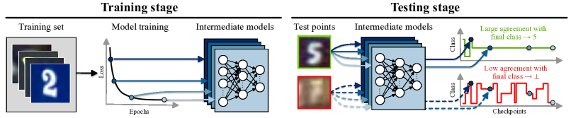
Figure 1: Our proposed NNTD method. During the model training stage, we store checkpoints of intermediate models. At inference time, given a test input, we compute various metrics capturing the agreement of intermediate predictions with the final model prediction. Data points with high agreement are accepted while data points with low agreement are rejected.

We derive the first framework for selective classification based on neural network training dynamics (see Figure 1). Typical DNNs are trained sequentially e.g., using stochastic gradient descent. Hence, as training goes on, the optimization process yields a sequence of intermediate models. In particular, because the goal of the optimization process is to learn a target label, the sequence of predictions these intermediate models yield on the points they optimized for should "converge" to a specific label. The question associated to our characterization of optimization is how to characterize/threshold what (with high probability) a "converged" sequence of predictions looks like while training. Our hypothesis is that after obtaining an appropriate characterization of predictions during training, the larger set of datapoints that also satisfy such a characterization overlaps significantly with the set of correctly predicted datapoints. So, determining the test points we optimized yields a performative selective classification method.

Through a formalization of this particular neural network training dynamics problem, we first note that a useful property of the intermediate models’ predictions is whether they agree with the final prediction. One can obtain a bound on how likely a given sequence of disagreements belongs to a point we optimized for if we know a priori the typical trend of disagreements. This leads to our characterization of being optimized. We empirically observe that the expected disagreement is almost always $0$ during training and the variance decreases in a convex manner.

These observations lead to our first proposed method to characterize optimizing a datapoint, and hence our first selective classification method, which imposes a threshold on the last model checkpoint whose prediction can disagree with the final model’s label prediction. However, this threshold could be very sensitive to the noise inherent in training. Hence, we propose a more robust characterization which thresholds a biased average over multiple intermediate models disagreeing with the final label prediction. This gives our second selective classification method. The latter method matches state-of-the-art accuracy/coverage trade-offs for selective classification. Again, we stress that our approach requires no modifications to existing training pipelines and is retroactively applicable to all models that have already been deployed. Our approach only requires that intermediate checkpoints were recorded when models were trained, which is an established practice.

Our main contributions are as follows:

1. We initiate studying selective classification through understanding the larger set of datapoints a model optimized (beyond the original training set).

2. We propose a novel method for SC based on neural network training dynamics (dubbed NNTD) in which we devise an effective scoring mechanism capturing the label disagreement of intermediate models with the final prediction for a particular test point. This method can be applied to all existing models whose checkpoints were recorded during training.

3. We perform a comprehensive set of empirical experiments on established SC benchmarks. Our results obtained with NNTD demonstrate a highly favorable accuracy/coverage of NNTD-based selective classification, matching state-of-the-art results in the field.

2 Background on Selective Classification

Our work considers the standard supervised multi-class classification setup. We assume to have access to a dataset $D=\{(\bm{x}_{i},y_{i})\}_{i=1}^{M}$ consisting of data points $(\bm{x},y)$ with $\bm{x}\in\mathcal{X}$ and $y\in\mathcal{Y}$. We refer to $\mathcal{X}=\mathbb{R}^{d}$ as the covariate space of dimensionality $d$ and $\mathcal{Y}=\{1,2,\ldots,C\}$ as the label space consisting of $C$ classes. All data points $(\bm{x},y)$ are sampled independently from the underlying distribution $p$ defined over $\mathcal{X}\times\mathcal{Y}$. Our goal is to learn a prediction function $f:\mathcal{X}\rightarrow\mathcal{Y}$ which minimizes the classification risk with respect to the underlying data distribution $p$ and an appropriately chosen loss function $\ell:\mathcal{Y}\times\mathcal{Y}\rightarrow\mathbb{R}$.

Setup

Selective classification alters the standard classification setup by introducing a rejection class $\bot$ through a gating mechanism (El-Yaniv and Wiener, 2010). In particular, such a mechanism introduces a selection function $g:\mathcal{X}\rightarrow\mathbb{R}$ which determines if a model should predict on a data point $\bm{x}$. Given an acceptance threshold $\tau$, the resulting predictive model can be summarized as:

$$(f,g)(\bm{x})=\begin{cases}f(\bm{x})&g(\bm{x})\geq\tau\\ \bot&\text{otherwise.}\end{cases}$$ (1)

Evaluation Metrics

Prior work evaluates the performance of a selective classifier $(f,g)$ based on two metrics: the coverage of $(f,g)$ (i.e., what fraction of points we predict on) and the accuracy of $(f,g)$ on the accepted points. Successful SC methods aim at obtaining both high accuracy and high coverage. Note that these two metrics are at odds with each other: naïvely increasing accuracy leads to lower coverage and vice-versa. The complete performance profile of a model can be specified using the risk–coverage curve, which defines the risk as a function of coverage (El-Yaniv and Wiener, 2010). These metrics can be formally defined as follows:

$$\text{cov}(f,g)=\frac{|\{\bm{x}:g(\bm{x})\geq\tau\}|}{|D|}\qquad\qquad\text{acc}(f,g)=\frac{|\{\bm{x}:f(\bm{x})=y,g(\bm{x})\geq\tau\}|}{|\{\bm{x}:g(\bm{x})\geq\tau\}|}$$ (2)

Past Work

The first work on SC for deep neural networks (DNNs) is the softmax response (SR) mechanism (Geifman and El-Yaniv, 2017). A threshold $\tau$ is applied to the maximum response of the softmax layer $\max_{y\in\mathcal{Y}}f(y|\bm{x})$. Given a confidence parameter $\delta$ and desired risk $r^{*}$, this creates a selective classifier $(f,g)$ whose test error is no larger than $r^{*}$ with probability of at least $1-\delta$. This approach however has been shown to produce over-confident results under mis-calibration (Guo et al., 2017). It was further shown by Lakshminarayanan et al. (2017) that model ensembles can improve upon the SR method. This however raises the need to train multiple models from scratch. Instead, in our work, we leverage intermediate models yielded during training to avoid the costly training of separate models to obtain an ensemble. A similar approach leveraging intermediate predictions is given by Huang et al. (2020) where intermediate predictions are incorporated into the loss function during training. In our method, however, we alleviate the need for training-time modifications while still leveraging intermediate predictions. As opposed to ensemble approaches, SelectiveNet (SN) (Geifman and El-Yaniv, 2019) trains a model to jointly optimize for classification and rejection. A loss penalty is added to enforce a coverage constraint using a variant of the interior point method. In a different approach, Deep Gamblers (DG) (Liu et al., 2019) transform the original $C$-class problem into a $(C+1)$-class problem where the additional class represents model abstention. Note that, while our method does not alter the training stage, both these methods introduce architectural or loss function changes. Other similar approaches include: abstention based on the variance statistics from several dropout-enabled forward passes (Gal and Ghahramani, 2016), performing statistical inference for the marginal prediction-set coverage rates using model ensembles (Feng et al., 2021), confidence prediction using an earlier snapshot of the model (Geifman et al., 2018), estimating the gap between classification regions corresponding to each class via One-Sided Prediction (Gangrade et al., 2021), and complete precision for SC via classifying only when models consistent with the training data predict the same output (Khani et al., 2016).

3 Our Method

We now introduce our selective classification algorithms based on neural network training dynamics. In Section 3.1 we introduce our motivating "optimized = correct (often)" hypothesis. Following this, we characterize what it means to have optimized the datapoint, which we ultimately will use as our selective classification algorithms. We refer to the class of methods we propose as NNTD.

3.1 An Intuition for our Method

Running SGD on different datasets could lead to the same final model (Hardt et al., 2016; Bassily et al., 2020; Thudi et al., 2022). For example, this is intuitive when two datasets were sampled from the same distribution. We would then expect that training on either dataset should not affect significantly the model returned by SGD. For our selective classification problem, this suggests an approach to decide which points the model is likely to predict correctly on: identify the datasets that it could have been trained on (in lieu of the training set it was actually trained on). In other words, give a method to check whether a given datapoint/dataset could have been used to train the model.

Prior work has proposed brute force approaches to this problem: e.g., Thudi et al. (2022) brute-forces through different mini-batches of data to see if a mini-batch can be used to reproduce one of the original training steps. Even then, this is only a sufficient condition to show a datapoint could have plausibly been used to train: if the brute-force fails, it does not mean the datapoint could not have been used to obtain the final model. As an alternative to this, we propose to instead characterize the optimization behaviour of training on a dataset, i.e conditions most datapoints that were (plausibly) trained on would satisfy based on training dynamics. Our modified hypothesis is then that the set of datapoints we optimized (for this notion of being optimized) coincides significantly with the set of points the model predicts correctly on.

3.2 A Framework for Being Optimized

We now build a framework for what variables (based on intermediate model states) can prove useful for characterizing the optimization behaviour while training. To do so, we derive an upper-bound on the probability that a datapoint could have been used to obtain the model’s checkpointing sequence. This yields a probabilistically necessary (though not sufficient) characterization of the points we explicitly optimized for. This bound, and the variables it depends on, informs what we will later use to characterize "optimizing" a datapoint, and, hence, our selective classification methods.

Let us denote the set of all datapoints as $\mathcal{D}$, and let $D^{\prime}\subset\mathcal{D}$ be the training set. We are interested in the setting where a model $f$ is plausibly sequentially trained on $D^{\prime}$ (e.g., with stochastic gradient descent). We thus also have access to a sequence of $T$ intermediate states for $f$, which we denote $\{f_{1},\cdots,f_{T}\}$. In this sequence, note that $f_{T}$ is exactly the final model $f$.

Now, let $p_{t}$ represent the random variable for outputs on $D^{\prime}$ given by an intermediate model $f_{t}$ where the outputs have been binarized: we have $0$ if the output agrees with the final prediction and $1$ if not. In other words, $p_{t}$ is the distribution of labels given by first drawing $\bm{x}\sim D^{\prime}$ and then outputting $1-\delta_{f_{t}(\bm{x}),f_{T}(\bm{x})}$ where $\delta$ denotes the Dirac delta function.

Note that we always have a well-defined mean and a well-defined variance for $p_{t}$ as it is bounded. Furthermore, we always have the variances and expectations of $\{p_{t}\}$ converge to $0$ with increasing $t$ (as $p_{T}=0$ always and the sequence is finite). To state this formally, let $v_{t}=\mathbb{V}[p_{t}]$ and $e_{t}=\mathbb{E}[p_{t}]$ denote the variances and expectations over points in $D^{\prime}$. In particular, we remark that $e_{T},v_{T}=0$, so both $e_{t}$ and $v_{t}$ converge. More formally, for all $\epsilon>0$ there exists an $N\in\{1,\ldots,T\}$ such that $v_{t}<\epsilon$ for all $t>N$. Similarly, for all $\epsilon>0$ there exists a (possibly different) $N\in\{1,\ldots,T\}$ such that $e_{t}<\epsilon$ for all $t>N$.

However, the core problem is that we do not know how this convergence in the variance and expectation occurs. More specifically, if we knew the exact values of $e_{t}$ and $v_{t}$, we could use the following bound on the probability of a particular data point being in $D^{\prime}$. We consequently introduce the notation $\{a_{1},\ldots,a_{T}\}$ where $a_{t}=1-\delta_{f_{t}(\bm{x}),f_{T}(\bm{x})}$ which we call the "label disagreement (at $t$)". Note that the $a_{t}$ are constants defined with respect to a given input, while $p_{t}$ represent the distribution of $a_{t}$ over all inputs in $D^{\prime}$.

Lemma 1.

Given a datapoint $\bm{x}$, let $\{a_{1},\ldots,a_{T}\}$ where $a_{t}=1-\delta_{f_{t}(\bm{x}),f_{T}(\bm{x})}$. Assuming not all $a_{t}=e_{t}$ then the probability $\bm{x}\in D^{\prime}$ is $\leq\min_{v_{t}~{}s.t~{}a_{t}\neq e_{t}}\frac{v_{t}}{|a_{t}-e_{t}|^{2}}$.

Proof.

By Chebyshev’s inequality we have the probability of a particular sequence $\{a_{1},\ldots,a_{T}\}$ occurring is $\leq\frac{v_{t}}{|a_{t}-\mathbb{E}(p_{t})|^{2}}$ for every $t$ (a bound on any of the individual $a_{t}$ occurring as that event is in the event $|p_{t}-e_{t}|\geq|a_{t}-e_{t}|$ occurs), and so taking the minimum over all these upper-bounds we obtain our upper-bound. ∎

We do not guarantee Lemma 1 is tight. Though we do take a minimum to make it tighter, this is a minimum over inequalities all derived from Markov’s inequality. Despite this potential looseness, using the bound from Lemma 1, we can design a naïve selective classification protocol based on the "optimized = correct (often)" hypothesis and use the above bound on being a plausible training datapoint as our characterization of optimization; for a test input $\bm{x}$, if the upper-bound on the probability of being a datapoint in $D^{\prime}$ is lower than some threshold $\tau$ reject, else accept. However, as mentioned earlier, we have the following two problems preventing us from readily using this method:

1. What is $\mathbb{E}[p_{t}]$ during training?

2. How does $\mathbb{V}[p_{t}]$ change during training?

These problems represent questions about how the predictions on plausibly training points evolve during training, i.e., training dynamics. More generally, they exemplify how a characterization of training dynamics could be useful for selective classification. Informally, the first problem represents knowing how often we predict the final label at step $t$, and the second problem represents knowing how we become more consistent as we continue training. Do note that the performance of this optimization-based approach to selective classification will depend on how unoptimized incorrect test points are. In particular, our hypothesis is that incorrect points often appear sufficiently unoptimized. We verify this behavior later in Section 4.3 where we discuss the distinctive label evolution patterns of optimized and correct datapoints versus incorrect test points.

The rest of this section will focus on the two methods we propose to characterize this optimization behaviour, giving rise to our selective classification methods. Although we do not give formal correctness guarantees for our methods for selective classification, or being a (with high probability) necessary condition to be a datapoint we explcitly optimized for, their design and assumptions are informed by Lemma 1 and by empirical estimates of $e_{t}$ and $v_{t}$ (later described in § 4.3).

3.3 The Minimum Score $s_{\text{min}}$

Here, we propose our first approach to characterizing optimizing a datapoint, i.e., our first selective classification algorithm. In what follows we will, after two simplifying assumptions, derive a candidate selective classification algorithm based off of Lemma 1.

In § 4.3 we observe that the expected values for the $p_{t}$ distribution from § 3.2, which we denote $e_{t}$, are near $0$ for most $t$; we will therefore further simplify our setup by assuming $e_{t}=0$ for all $t$. Note that if $e_{t}=0$ and the label disagreement $a_{t}=1$, then $\frac{v_{t}}{|a_{t}-\mathbb{E}[p_{t}]|^{2}}=v_{t}$. So based on Lemma 1, assuming $e_{t}=0$ for all $t$, the measure for acceptance we are interested in is $s_{\text{min}}=\min_{t~{}s.t~{}a_{t}=1}v_{t}$. Note now $s_{\text{min}}$ depends on what $v_{t}$ are. From § 4.3 we observe $v_{t}$ monotonically decrease in a convex manner. Thus, we choose to approximate the empirical trend observed in § 4.3 with $v_{t}=1-t^{k}$ (for $k\in(0,1]$), which also decrease in a convex manner.

Our first algorithm for selective classification is hence given by:

1. Denote $L=f_{T}(\bm{x})$, i.e. the label our final model predicts.

2. If $\exists t~{}s.t~{}a_{t}=1$ then compute $s_{\text{min}}=\min_{t~{}s.t~{}a_{t}=1}v_{t}$ as per the notation in § 3.2 (i.e $a_{t}=1$ iff $f_{t}(x)\neq L$), else accept $\bm{x}$ with prediction $L$.

3. If ${\color[rgb]{0,0,0}s_{\text{min}}}>\tau$ accept $\bm{x}$ with prediction $L$, else reject ($\bot$).

Intuitively, as all our candidate $v_{t}$ decrease, the algorithm imposes a last intermediate model which can output a prediction that disagrees with the final prediction: hereafter, the algorithm must output models that consistently agree with the final prediction. The effectiveness of this method for selective classification depends on how quickly $v_{t}$ decrease (assuming $e_{t}=0$ always) as opposed to the variance for incorrect data points. In particular, if there was an index $N$ such that for $t>N$, we have that $f_{t}(x)=f_{T}(x)$ for correctly classified points, but never (or rarely) for incorrectly classified points, then this method would successfully separate the correct from the incorrect.

3.4 The Average Score $s_{\text{avg}}$

Note that the previous characterization of optimization, defined by the score $s_{\text{min}}$, could be sensitive to stochasticity in training and hence perform sub-optimally. In particular, this algorithm could be noisy for different training runs (of otherwise identical models) as $\min_{t~{}s.t~{}a_{t}=1}v_{t}$ could vary drastically based on the exact sequence of mini-batches used during training.

In light of this potential limitation we propose the following "averaging" algorithm:

1. Denote $L=f_{T}(\bm{x})$, i.e. the label our final model predicts.

2. If $\exists t~{}s.t~{}a_{t}=1$, compute $s_{\text{avg}}=\frac{\sum v_{t}a_{t}}{\sum a_{t}}$, else accept $\bm{x}$ with prediction $L$.

3. If ${\color[rgb]{0,0,0}s_{\text{avg}}}>\tau$ accept $\bm{x}$ with prediction $L$, else reject ($\bot$).

Intuitively, recalling our previous candidates for $v_{t}$, $s_{\text{avg}}$ computes a weighted average. In particular, we are adding little weight to later disagreements with the final prediction while still increasing the denominator by the same amount. In § 4, we show that $s_{\text{avg}}$ leads to considerably more robust selective classification results compared to $s_{\text{min}}$.

4 Empirical Evaluation

Table 1: Performance at low target errors. Our NNTD$(s_{\text{avg}},0.05)$ method either matches or provides higher coverage levels of the test set at a fixed target error than other competing methods. Bold entries are within one standard deviation over 5 random runs (standard deviations in Table 9).

Dataset	Target	NNTD		SAT		DG		SN		SR		MC-DO
	Error	Cov $\uparrow$	Err	Cov $\uparrow$	Err	Cov $\uparrow$	Err	Cov $\uparrow$	Err	Cov $\uparrow$	Err	Cov $\uparrow$	Err
CIFAR-10	2%	91.2	1.99	90.3	1.97	89.1	2.02	88.3	2.03	85.8	1.98	86.1	2.01
	1%	86.4	1.00	86.1	1.02	85.5	1.03	84.4	0.98	79.1	1.01	79.9	1.01
	0.5%	75.9	0.49	76.0	0.51	75.2	0.51	74.7	0.49	71.2	0.51	72.0	0.50
SVHN	2%	98.5	1.98	98.2	1.99	97.8	2.06	97.7	2.03	97.6	1.99	97.9	2.00
	1%	96.3	0.99	95.7	1.03	94.8	0.99	94.5	1.04	93.5	1.01	94.1	0.97
	0.5%	88.1	0.50	87.9	0.51	86.4	0.51	86.0	0.51	70.0	0.50	70.1	0.49
Cats & Dogs	2%	97.7	2.01	98.2	1.98	98.0	2.03	97.4	1.98	95.1	1.99	95.7	1.99
	1%	93.1	1.01	93.6	0.98	92.6	0.97	92.2	0.98	86.9	0.98	88.6	1.01
	0.5%	85.7	0.51	86.0	0.49	85.3	0.49	84.8	0.46	68.4	0.48	70.1	0.51

Table 2: Performance at high target coverage. Similar as shown in Table 1, NNTD$(s_{\text{avg}},0.05)$ matches or outperforms SOTA error rates at fixed coverage levels (standard deviations in Table 10).

Dataset	Target	NNTD		SAT		DG		SN		SR		MC-DO
	Coverage	Cov	Err $\downarrow$	Cov	Err $\downarrow$	Cov	Err $\downarrow$	Cov	Err $\downarrow$	Cov	Err $\downarrow$	Cov	Err $\downarrow$
CIFAR-10	100%	100	6.07	100	6.06	100	6.11	100	6.13	100	6.07	100	6.07
	95%	95.0	3.24	95.1	3.32	95.1	3.47	95.0	4.08	94.9	4.48	95.1	4.48
	90%	90.1	1.83	89.9	1.90	90.0	2.19	90.1	2.29	90.1	2.78	90.0	2.87
	80%	79.9	0.64	80.0	0.65	80.1	0.66	80.1	0.81	79.8	1.05	79.9	1.01
	70%	69.8	0.34	69.9	0.32	69.8	0.41	70.2	0.30	70.0	0.47	70.1	0.42
SVHN	100%	100	2.68	100	2.71	100	2.72	100	2.77	100	2.68	100	2.68
	95%	95.0	0.88	95.1	0.95	95.1	1.01	95.0	1.07	94.9	1.15	95.1	1.12
	90%	90.1	0.55	89.9	0.58	90.0	0.63	90.1	0.71	90.1	0.82	90.0	0.76
	80%	79.9	0.38	80.0	0.37	80.1	0.43	80.1	0.48	79.8	0.55	79.9	0.53
	70%	69.8	0.33	69.9	0.33	69.8	0.35	70.2	0.45	70.0	0.50	70.1	0.49
Cats & Dogs	100%	100	3.48	100	3.45	100	3.41	100	3.56	100	3.48	100	3.48
	95%	95.1	1.51	95.1	1.45	95.0	1.43	94.9	1.61	94.8	1.92	95.1	1.95
	90%	90.1	0.60	89.9	0.57	90.0	0.69	90.1	0.95	90.1	1.13	90.0	1.09
	80%	79.9	0.42	80.0	0.41	80.1	0.56	80.1	0.39	79.8	0.69	79.9	0.58
	70%	69.8	0.36	69.9	0.33	69.8	0.45	70.2	0.33	70.0	0.62	70.1	0.51

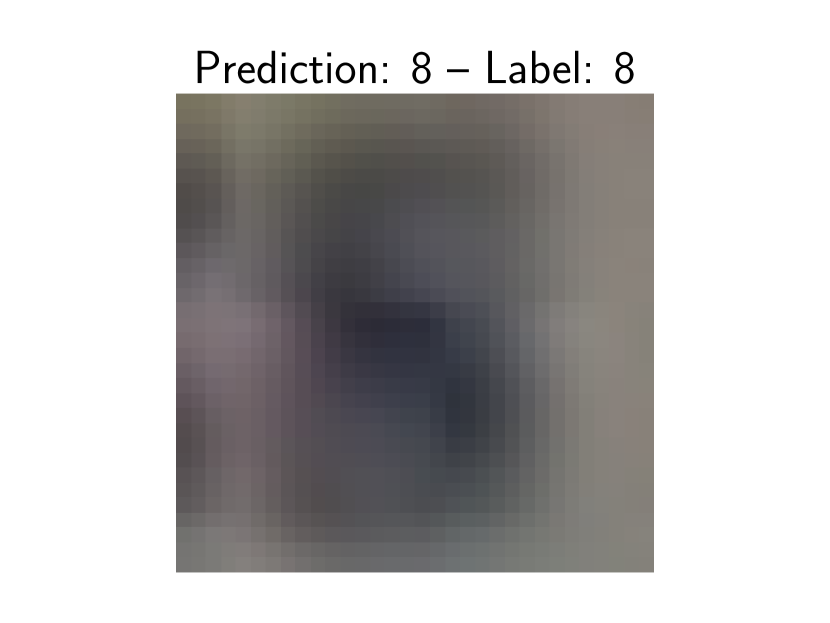
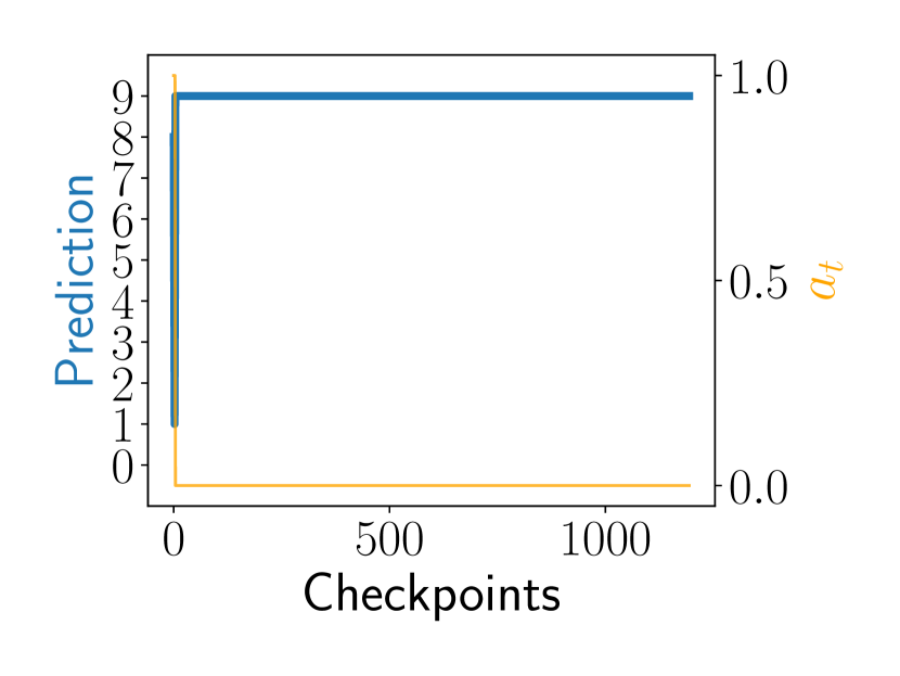
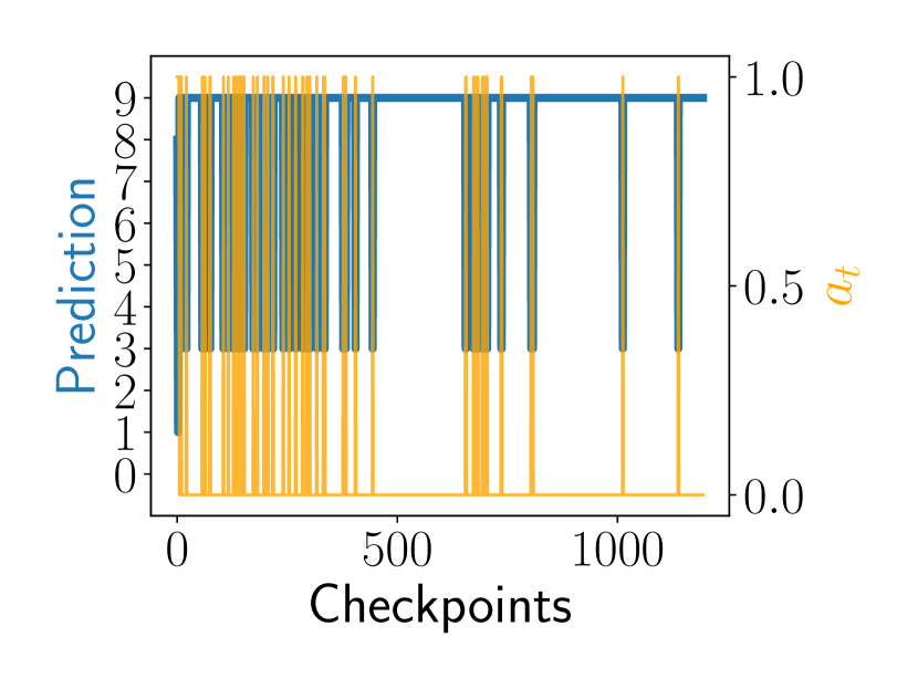
Figure 2: Individual SVHN examples. In the first row, we show four examples from the SVHN test set. For each example we plot both the prediction evolution and the final label agreement metric $a_{t}$ over all checkpoints in the second row. We note that the first two examples are easy to classify as indicated by a mostly stationary prediction curve, while the last two examples are harder to classify since the prediction is highly unstable across intermediate models.

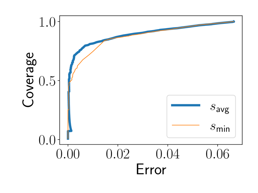
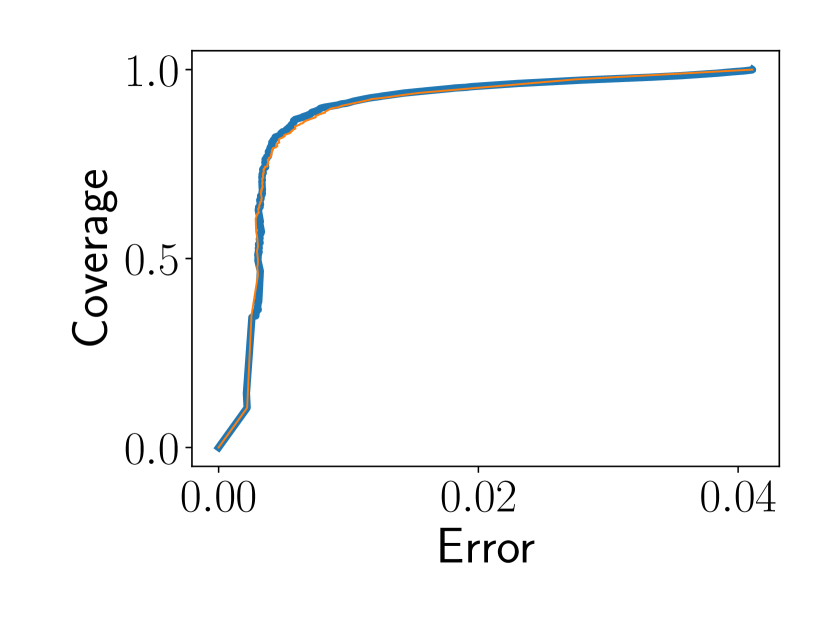
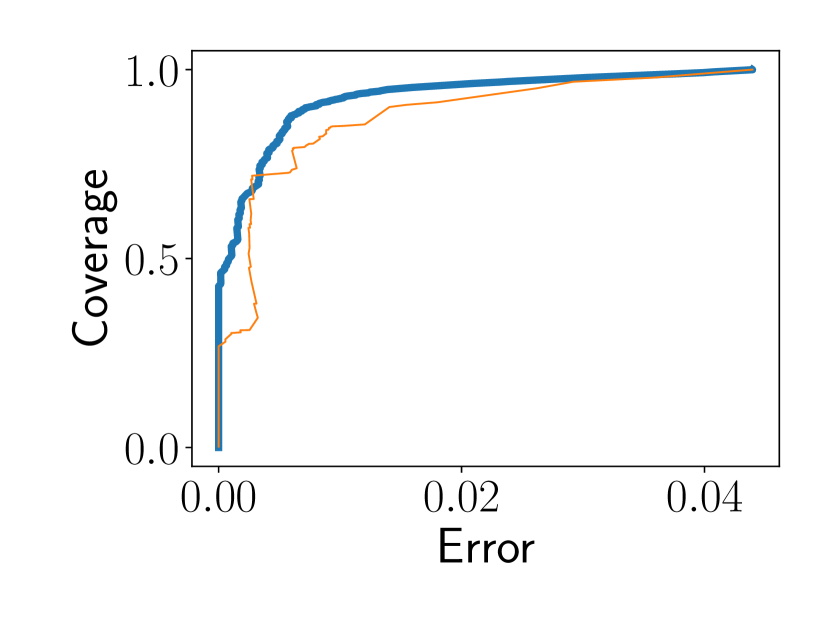
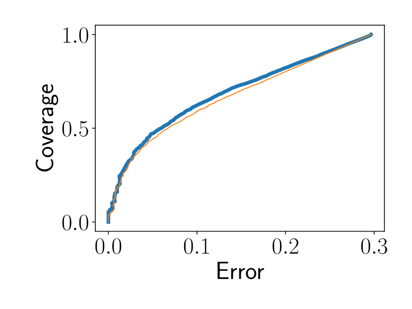
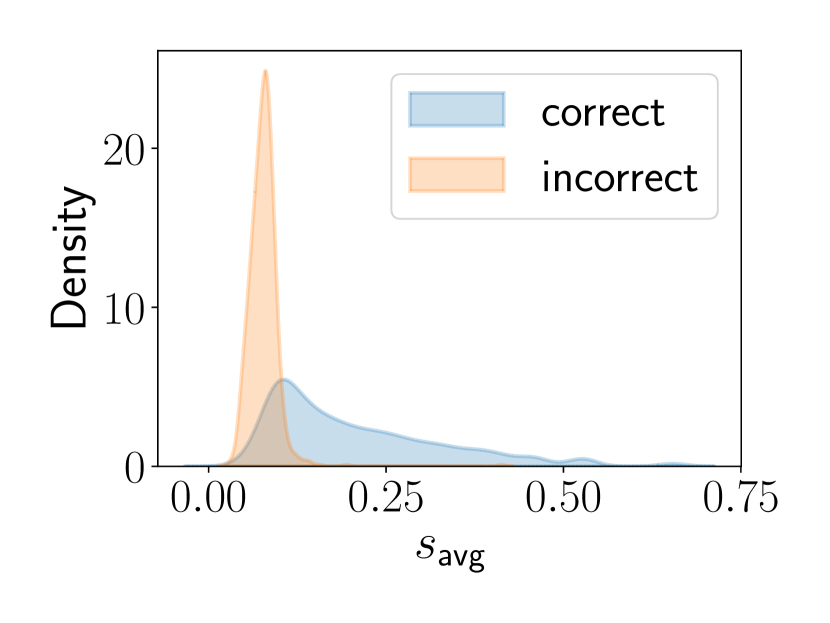
(a) CIFAR-10

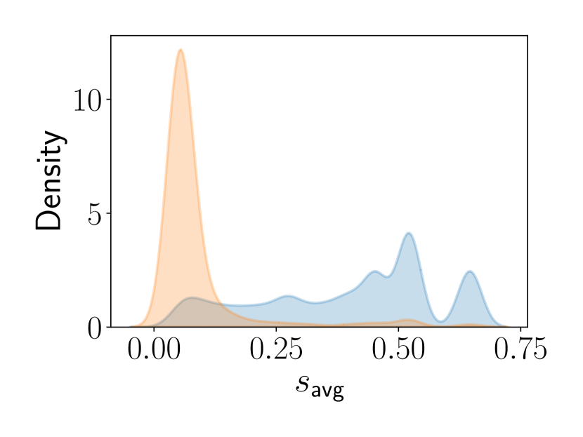
(b) SVHN

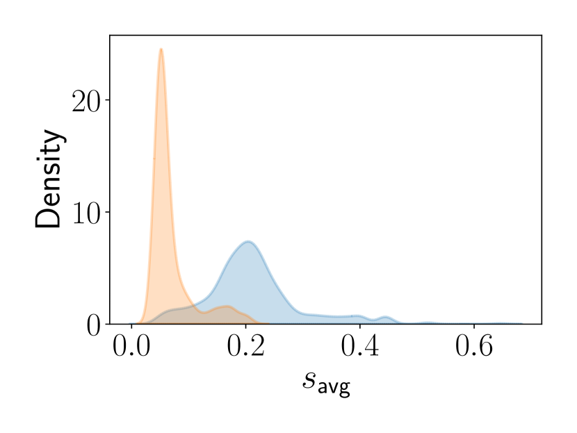
(c) GTSRB

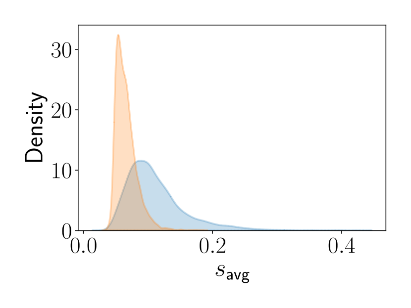
(d) CIFAR-100

Figure 3: Performance and distribution of our metrics for different datasets. The first row shows the coverage/error curves for $s_{\text{min}}$ and $s_{\text{avg}}$. We show the distribution of the average score metric $s_{\text{avg}}$ for both correctly and incorrectly classified samples in the second row.

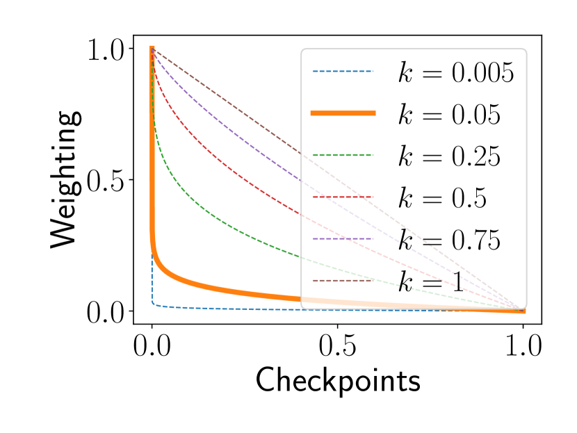
(a) Convex weighting

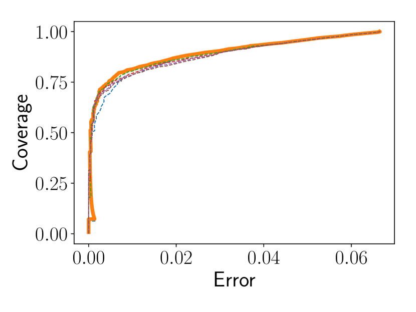
(b) CIFAR-10

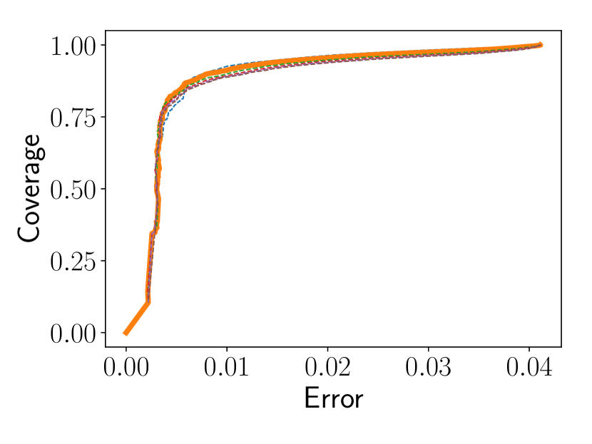
(c) SVHN

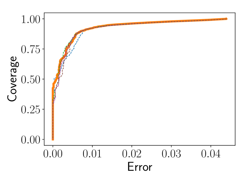
(d) GTSRB

Figure 4: Convex weighting used in $v_{t}=1-t^{k}$. Overall, we find that NNTD ($s_{\text{avg}}$,$k$) is generally robust to the exact choice of $k$ and $k=0.05$ performs best across our experiments.

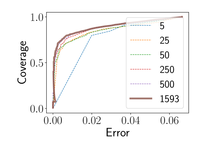
(a) CIFAR-10

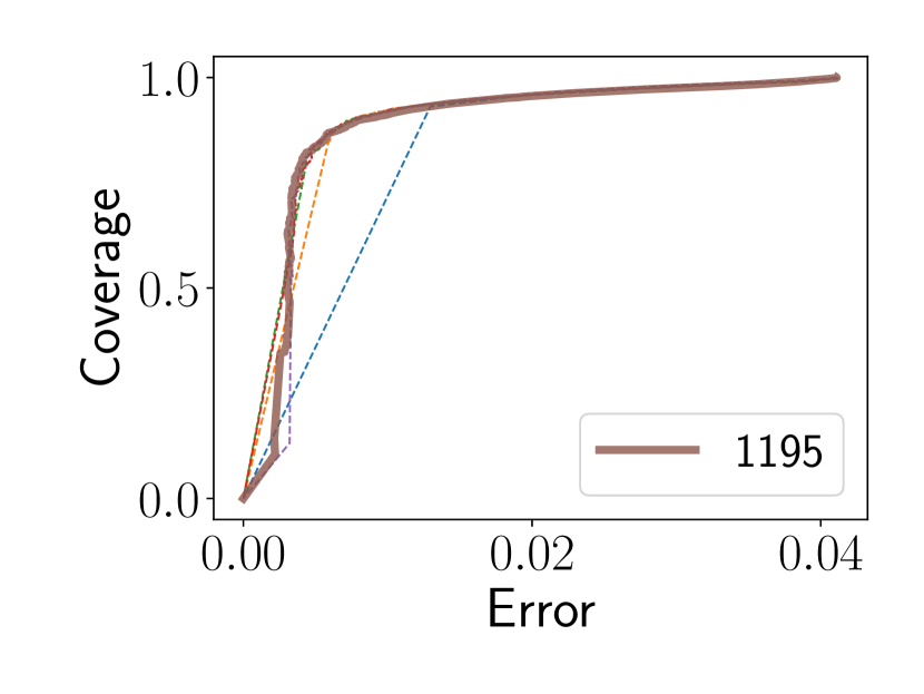
(b) SVHN

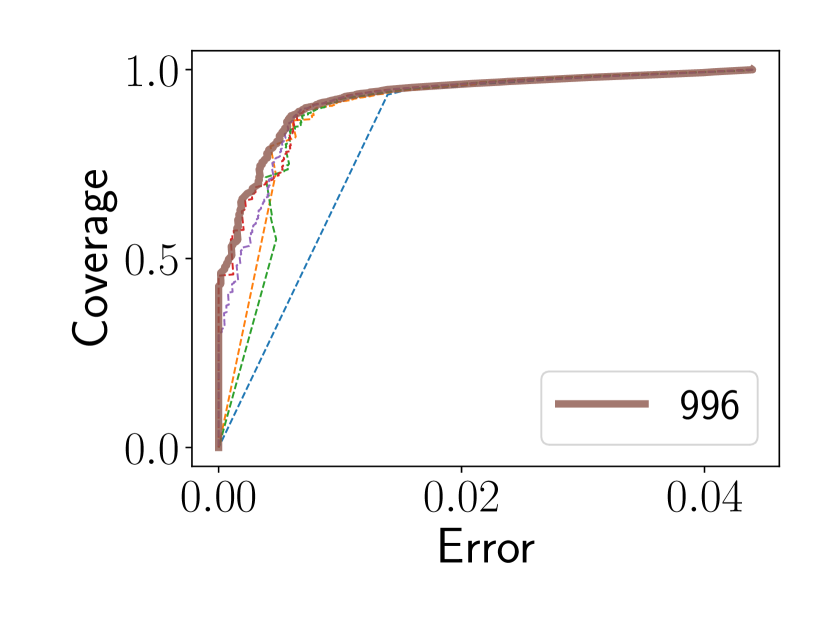
(c) GTSRB

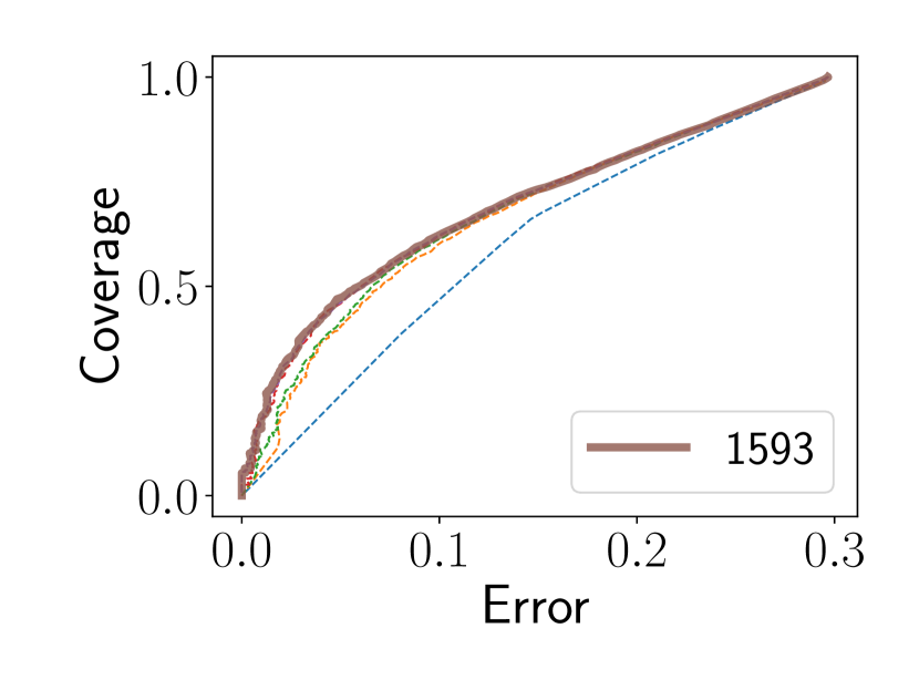
(d) CIFAR-100

Figure 5: Coverage/error trade-off of NNTD$(s_{\text{avg}},0.05)$ for various checkpointing resolutions. Overall, we find that using 25-50 checkpoints already offers very competitive results. Using multiple hundreds of checkpoints offers diminishing returns but improves coverage at low error rates.

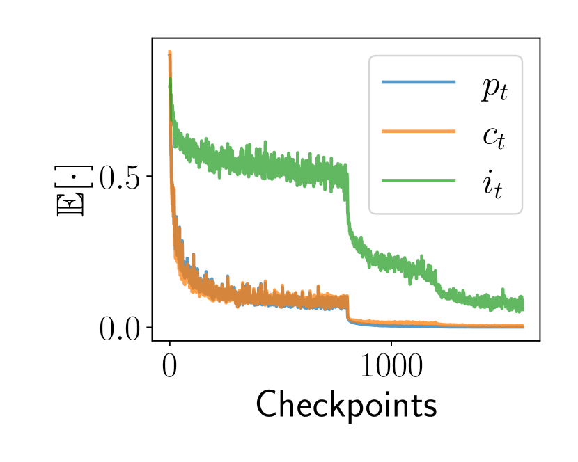
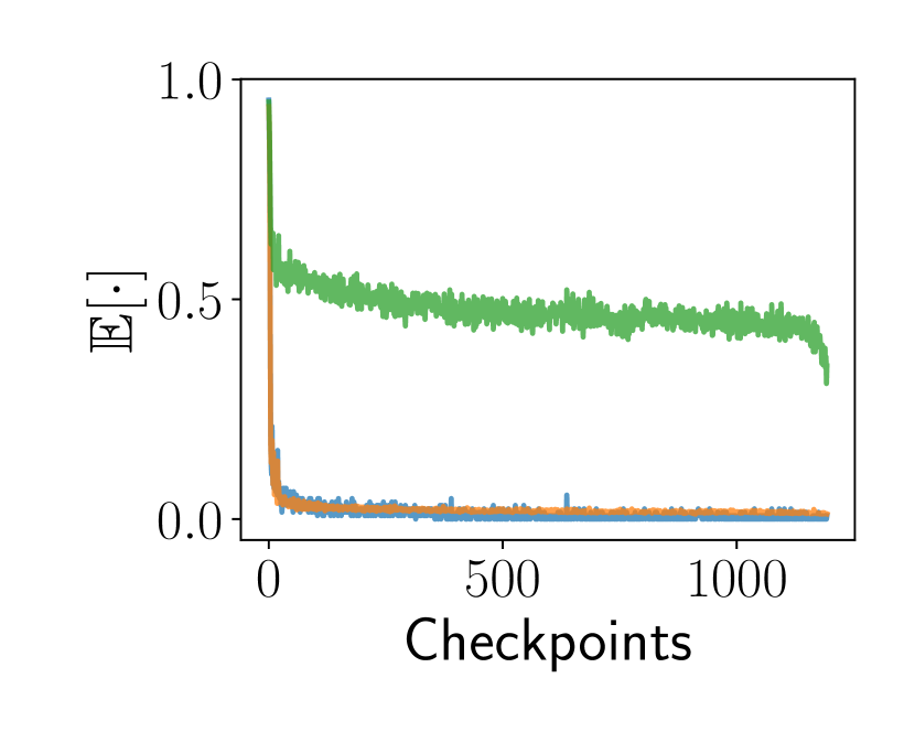
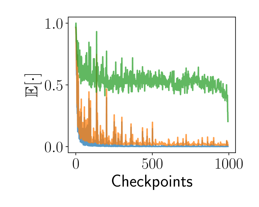
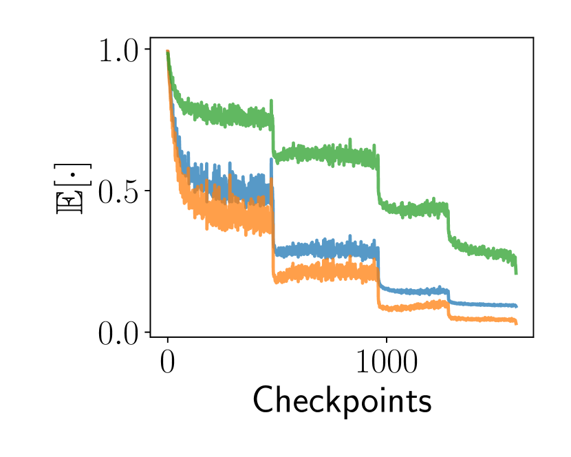
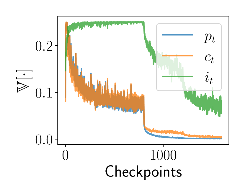
(a) CIFAR-10

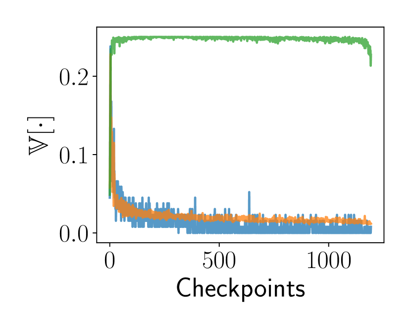
(b) SVHN

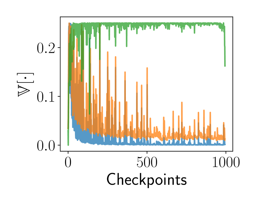
(c) GTSRB

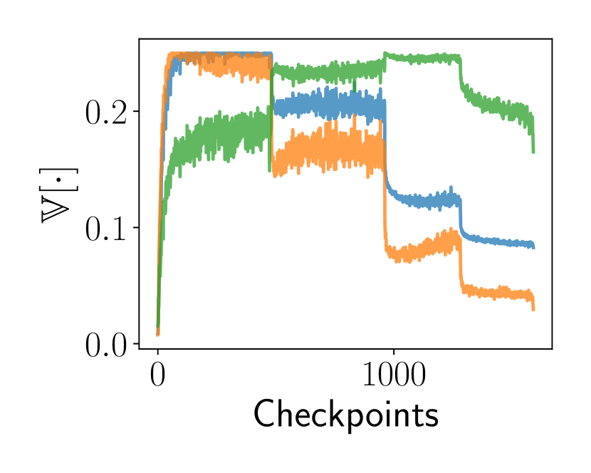
(d) CIFAR-100

Figure 6: Monitoring $\mathbb{E}[\cdot]$ and $\mathbb{V}[\cdot]$ for training points ($p_{t}$) and both correctly ($c_{t}$) and incorrectly ($i_{t}$) classified test points. We see that the patterns for optimized points overlaps significantly with correctly classified test-time points. In particular, correctly classified points have both their expectations and variances quickly decreasing to 0 as training progresses. Incorrectly classified points both exhibit large expectations and variances and stay constant over large periods while training.

4.1 Setup

Datasets & Training

We evaluate our proposed approach on image dataset benchmarks that are common in the selective classification literature: CIFAR-10/CIFAR-100 (Krizhevsky et al., 2009), SVHN (Netzer et al., 2011), Cats & Dogs, and GTSRB (Houben et al., 2013). For each dataset, we train a deep neural network following the VGG16 architecture (Simonyan and Zisserman, 2014) (using batch normalization and dropout) and checkpoint each model after processing 50 mini-batches of size 128. All models are trained over 300 epochs using the SGD optimizer with an initial learning rate of $10^{-1}$, momentum $0.9$, and weight decay $10^{-4}$. For CIFAR-10 (CIFAR-100), we reduce the learning rate by 0.5 after 100 (50, 100, and 150) epoch(s), respectively. To facilitate comparison with prior work, we match the accuracy of our models at the levels provided in Huang et al. (2020).

Baselines

We compare our method based on neural network training dynamics (NNTD) to 5 common SC techniques previously introduced in § 2: Softmax Response (SR) (Geifman and El-Yaniv, 2017), SelectiveNet (SN) (Geifman and El-Yaniv, 2019), Deep Gamblers (DG) (Liu et al., 2019), Self-Adaptive Training (SAT) (Huang et al., 2020), and Monte-Carlo Dropout (MC-DO) (Gal and Ghahramani, 2016). We further compare against One-Sided Prediction (OSP) (Gangrade et al., 2021) in Appendix C.1. Our hyper-parameter tuning procedure is documented in Appendix C.2.

4.2 Results

Our empirical results show that computing and thresholding the average score $s_{\text{avg}}$ using weighting parameter $k=0.05$ provides a strong score for selective classification. We denote this method NNTD$(s_{\text{avg}},0.05)$. In the following, we first study the accuracy/coverage trade-off with comparison to past work. Then, we present exemplary label evolution curves for individual SVHN examples. Finally, we analyze the performance of the metrics proposed in § 3 in depth and examine our method’s sensitivity to the checkpoint selection strategy and the weighting parameter $k$.

Accuracy/Coverage Trade-off

Consistent with standard evaluation schemes for selective classification, our main experimental results examine the accuracy/coverage trade-off of NNTD$(s_{\text{avg}},0.05)$. We present our main performance results with comparison to past work in Tables 1 and 2 where we demonstrate NNTD’s effectiveness on CIFAR-10, SVHN, and Cats & Dogs. In Table 1, we document the results obtained by NNTD, SAT, SR, SN, DG, and MC-DO for a fixed low target error $e\in\{2\%,1\%,0.5\%\}$. In Table 2, we follow a similar setup but instead of fixing the target error we evaluate all methods for a fixed high target coverage $c\in\{100\%,95\%,90\%,80\%,70\%\}$. We see that NNTD either matches or outperforms existing state-of-the-art selective classification methods.

Individual Evolution Plots

To analyze the behavior of the metrics proposed in Section 3, we examine label prediction evolution curves for individual SVHN examples in Figure 2 (more examples provided in Appendix C.3). In particular, we select two easy-to-classify examples and two ambiguous examples from the test set and plot both the prediction evolution and the final label agreement metric $a_{t}$ over all checkpoints. We observe that easy examples only show a small degree of oscillation while hard examples show more erratic patterns. This result matches our intuition: our model should produce correct decisions on data points whose prediction is mostly constant throughout training and should reject data points for which intermediate models predict inconsistently.

Choice of Metric

As per our theoretical framework and intuition provided in § 3, the average score $s_{\text{avg}}$ should offer the most competitive selective classification performance. We confirm this finding in Figure 3 where we plot the coverage/error curves for CIFAR-10, SVHN, GTSRB, and CIFAR-100 for both $s_{\text{min}}$ and $s_{\text{avg}}$. Overall, we find that the average score $s_{\text{avg}}$ consistently outperforms the more noisy minimum score $s_{\text{min}}$. We also show that $s_{\text{avg}}$ yields distinct distributional patterns for both correctly and incorrectly classified points. This separation enables strong coverage/accuracy trade-offs via our thresholding procedure.

Checkpoint weighting sensitivity

One important hyper-parameter of our method is the weighting of intermediate predictions. Recall from § 3 that NNTD makes use of a convex weighting function $v_{t}=1-t^{k}$. In Figure 4, we observe that NNTD$(s_{\text{avg}},k)$ is generally robust to the exact choice of $k$ and that $k=0.05$ performs best. At the same time, we find that decreasing $k$ too much leads to a decrease in coverage at fixed accuracy levels. This result confirms that (i) large parts of the training process contain valuable signals for selective classification; and that (ii) early label disagreements should be de-emphasized by our method.

Checkpoint selection strategy

The second important hyper-parameter of our method is the checkpoint selection strategy. In particular, to reduce computational cost, we study the sensitivity of NNTD$(s_{\text{avg}},0.05)$ with respect to the checkpointing resolution in Figure 5. Our experiments demonstrate favorable coverage/error trade-offs at 25-50 checkpoints. Further increasing the resolution to hundreds of intermediate models does offer diminishing returns but also leads to better coverage especially at very low error rates. We investigate alternative selection strategies in Appendix C.3.6.

4.3 Examining the Convergence Behavior of Training and Test Points

As alluded to in the assumptions presented in § 3.2, we hypothesize that training points (which we use to characterize optimization) and correctly classified test points share similar label convergence behavior. At the same time, incorrectly classified points should show different evolution patterns. We verify this hypothesis in Figure 6 and observe that the expected label disagreement for both training and correctly classified points are $0$ for large time periods, with a sudden initial drop from near $1$ to $0$; this drop becomes elongated for more challenging data sets such as CIFAR-10 and CIFAR-100 (for which the learning rate scheduling is visible in the plot). We also see that the variances follow an analogous decreasing trend. In general, both training points $p_{t}$ and correctly classified test points $c_{t}$ converge monotonically (and convexly) to $0$. In contrast, incorrectly classified points $i_{t}$ show significantly larger mean and variance levels.

5 Conclusion

We propose a new method for selective classification that matches the current state-of-the-art, but importantly can be applied to all existing models whose checkpoints were recorded (hence having the potential for immediate impact). This method came from the hypothesis that the set of datapoints we optimized often coincides with the set of correct datapoints; hence, methods to verify if a test point was sequentially optimized are also effective selective classification methods. We believe future work can improve our approach by investigating cases where our hypothesis did not hold for our characterization of optimization. For example, a model could predict correctly on a datapoint despite the intermediate predicted labels never converging. Similarly, a datapoint could have been optimized, but the labels converged to the wrong label.

Ethics Statement

Modern neural networks often produce overconfident decisions (Guo et al., 2017). This limitation, amongst other shortcomings, prevents neural nets from being readily applied in high-stakes decision-making. Selective classification is one paradigm enabling the rejection of data points. In particular, samples that would most likely be misclassified should be rejected. Since our work improves over current state-of-the-art methods, our work can be used to enhance the trustworthiness of deep neural networks in practice. While modern selective classification techniques mitigates overconfidence, recent work has also shown that SC algorithms disproportionately reject samples from minority groups (Jones et al., 2020). This finding suggests that improvements to the overall coverage comes at a fairness cost. As a result, the connection between fairness and sample rejection still warrants further investigation.

Reproducibility Statement

In accordance with contemporary works on selective classifciation, our experimental setup uses widely used and publicly accessible datasets from the vision domain. Baseline results were obtained using open-source implementations of the respective papers as published by the authors. Hyper-parameter tuning is performed as described in original works and documented in Appendix C.2. Moreover, our method implementation will be open sourced as part of the reviewing process.

Appendix A Connection to Example Difficulty

A related line of work is identifying difficult examples, or how well a model can generalize to a given unseen example. Jiang et al. (2020) introduce a per-instance empirical consistency score which estimates the probability of predicting the ground truth label with models trained on data subsamples of different sizes. Unlike our approach, however, this requires training a large number of models.  Toneva et al. (2018) quantifies example difficulty through the lens of a forgetting event, in which the example is misclassified after being correctly classified. However, the metrics that we introduce in § 3, are based on the disagreement of the label at each checkpoint with the final predicted label. Other approaches estimate the example difficulty by: prediction depth of the first layer at which a $k$-NN classifier correctly classifies an example (Baldock et al., 2021), the impact of pruning on model predictions of the example (Hooker et al., 2019), and estimating the leave-one-out influence of each training example on the accuracy of an algorithm by using influence functions (Feldman and Zhang, 2020). Closest to our method, the work of Agarwal et al. (2020) utilizes gradients of intermediate models during training to rank examples by difficulty. In particular, they average pixel-wise variance of gradients for each given input image. Notably, this approach is more costly and less practical than our approach and also does not study the accuracy/coverage trade-off which is of paramount importance to SC.

Appendix B Alternative Metric Choices

We briefly discuss additional potential metric choices that we investigated but which lead to SC performance worse than $s_{\text{avg}}$. A more elaborate discussion of these results is provided in Appendix C.3.

B.1 Incorporating Estimates of $e_{t}$ into $s_{\text{min}}$ and $s_{\text{avg}}$

Since the results in § 4.3 show that $e_{t}$ is only nearly $0$ almost everywhere, we investigate whether incorporating an estimate of $e_{t}$ into $s_{\text{min}}$ and $s_{\text{avg}}$ leads to additional SC improvements. Our results demonstrate that neither an empirical estimate nor a smooth decay function similar to $v_{t}$ robustly improves over $s_{\text{min}}$ and $s_{\text{avg}}$ (which assumed $e_{t}=0$).

B.2 Jump Score $s_{\text{jmp}}$

We also consider a score which captures the level of disagreement between the predicted label of two successive intermediate models (i.e., how much jumping occurred over the course of training). For $j_{t}=0$ iff $f_{t}(\bm{x})=f_{t-1}(\bm{x})$ and $j_{t}=1$ otherwise we can compute the jump score as $s_{\text{jmp}}=1-\sum v_{t}j_{t}$ and threshold it as in § 3.3 and § 3.4.

B.3 Variance Score $s_{\text{var}}$ for Continuous Metrics

Finally, we consider monitoring the evolution of continuous metrics that have been shown to be correlated with example difficulty. More specifically, Jiang et al. (2020) show that example difficulty is correlated with confidence and negative entropy. Moreover, they find that difficult examples are learned later in the training process. This observation motivates designing a score based on these continuous metrics that penalises changes later in the training process more heavily. We consider the maximum softmax class probability known as confidence, the negative entropy and the gap between the most confident classes for each example instead of the model predictions. Assume that any of these metrics is given by a sequence $z=\{z_{1},\ldots,z_{T}\}$ obtained from $T$ intermediate models. Then we can capture the uniformity of $z$ via a (weighted) variance score $s_{\text{var}}=\sum_{t}w_{t}(z_{t}-\mu)^{2}$ for mean $\mu=\frac{1}{T}\sum_{t}z_{t}$ and an increasing weighting sequence $w=\{w_{1},\ldots,w_{T}\}$.

In order to show the effectiveness of the variance score $s_{\text{var}}$ for continuous metrics, we provide a simple bound on the variance of confidence $\max_{y\in\mathcal{Y}}f_{t}(\bm{x})$ in the final checkpoints of the training. Assuming that the model has converged to a local minima with a low learning rate, we can assume that the distribution of model weights can be approximated by a Gaussian distribution.

We consider a linear regression problem where the inputs are linearly separable.

Lemma 2.

Assume that we have some Gaussian prior on the model parameters in the logistic regression setting across $m$ final checkpoints. More specifically, given $T$ total checkpoints of model parameters $\{\bm{w}_{1},\bm{w_{2}},\dots,\bm{w}_{T}\}$ we have $p(W=\bm{w}_{t})=\mathcal{N}(\bm{w}_{0}\mid\bm{\mu},s\bm{I})$ for $t\in\{T-m+1,\dots,T\}$ and we assume that final checkpoints of the model are sampled from this distribution. We show that the variance of model confidence $\max_{y\in\{-1,1\}}p(y\mid\bm{x}_{i},\bm{w}_{t})$ for a datapoint $(\bm{x}_{i},y_{i})$ can be upper bounded by a factor of probability of correctly classifying this example by the optimal weights.

Proof.

We first compute the variance of model predictions $p(y_{i}\mid\bm{x}_{i},W)$ for a given datapoint $(\bm{x}_{i},y_{i})$. Following previous work (Schein and Ungar, 2007; Chang et al., 2017), the variance of predictions over these checkpoints can be estimated as follows:

Taking two terms in Taylor expansion for model predictions we have $p(y_{i}\mid\bm{x}_{i},W)\simeq p(y_{i}\mid\bm{x}_{i},\bm{w})+g_{i}(\bm{w})^{\top}(W-\bm{w})$ where $W$ and $\bm{w}$ are current and the expected estimate of the parameters and $g_{i}(\bm{w})=p(y_{i}\mid\bm{x}_{i},\bm{w})(1-p(y_{i}\mid\bm{x}_{i},\bm{w}))\bm{x}_{i}$ is the gradient vector. Now we can write the variance with respect to the model prior as:

$$\mathbb{V}\left(p(y_{i}\mid\bm{x}_{i},W)\right)\simeq\mathbb{V}\left(g_{i}(\bm{w})^{\top}(W-\bm{w})\right)=g_{i}(\bm{w})^{\top}F^{-1}g_{i}(\bm{w})$$

where $F$ is the variance of posterior distribution $p(W\mid X,Y)\sim\mathcal{N}(W\mid\bm{w},F^{-1})$. This suggests that the variance of probability of correctly classifying $\bm{x}_{i}$ is proportional to $p(y_{i}\mid\bm{x}_{i},\bm{w})^{2}(1-p(y_{i}\mid\bm{x}_{i},\bm{w}))^{2}$. Now we can bound the variance of maximum class probability or confidence as below:

$$\mathbb{V}\left(\max_{y\in\{-1,1\}}p(y\mid\bm{x}_{i},W)\right) \leq\mathbb{V}\left(p(y_{i}\mid\bm{x}_{i},W)\right)+\mathbb{V}\left(p(-y_{i}\mid\bm{x}_{i},W)\right)$$

$$\approx 2p(y_{i}\mid\bm{x}_{i},\bm{w})^{2}(1-p(y_{i}\mid\bm{x}_{i},\bm{w}))^{2}\bm{x}_{i}^{\top}F^{-1}\bm{x}_{i}$$

∎

We showed that if the probability of correctly classifying an example given the final estimate of model parameters is close to one, the variance of model predictions following a Gaussian Prior gets close to zero, we expect a similar behaviour for the variance of confidence under samples of this distribution.

Appendix C Extension of Empirical Evaluation

C.1 Comparison with One-Sided Prediction

In addition to the main results, we also compare NNTD to one-sided prediction (OSP). For this set of experiments, we evaluate our proposed approach on image dataset benchmarks that are common in the selective classification literature: CIFAR-10, SVHN, and Cats & Dogs. For each dataset, we train a deep neural network following the ResNet-32 architecture (He et al., 2016) and checkpoint each model after processing 50 mini-batches of size 128. All models are trained over 200 epochs. SVHN, Cats & Dogs, and GTSRB are trained using the Adam optimizer with learning rate $10^{-3}$. The CIFAR-10 and CIFAR-100 models are trained using momentum-based stochastic gradient descent with an initial learning rate of $10^{-1}$ on a multi-step learning rate reduction schedule (reduction by $10^{-1}$ after epochs 100 and 150), momentum $0.9$, and weight decay $10^{-4}$. We report these results in Tables 3 and 4.

Table 3: Performance at low target errors for OSP based setup. Our NNTD$(s_{\text{avg}},0.05)$ method either matches or provides higher test set coverage at a fixed target error than other competing methods. Bold entries are within one standard deviation of each other over 5 random runs.

Dataset	Target	NNTD		OSP		SR		SN		DG
	Error	Cov.	Error	Cov.	Error	Cov.	Error	Cov.	Error	Cov.	Error
CIFAR-10	2%	83.3	1.96	80.6	1.91	75.1	2.09	73.0	2.31	74.2	1.98
	1%	79.7	1.05	74.0	1.02	67.2	1.09	64.5	1.02	66.4	1.01
	0.5%	74.2	0.49	64.1	0.51	59.3	0.53	57.6	0.48	57.8	0.51
SVHN	2%	95.7	1.96	95.8	1.99	95.7	2.06	93.5	2.03	94.8	1.99
	1%	91.2	0.99	90.1	1.03	88.4	0.99	86.5	1.04	89.5	1.01
	0.5%	83.9	0.50	82.4	0.51	77.3	0.51	79.2	0.51	81.6	0.49
Cats & Dogs	2%	90.5	2.03	90.5	1.98	88.2	2.03	84.3	1.94	87.4	1.94
	1%	85.6	1.01	85.4	0.98	80.2	0.97	78.0	0.98	81.7	0.98
	0.5%	77.5	0.50	78.7	0.49	73.2	0.49	70.5	0.46	74.5	0.48

Table 4: Performance at high target coverage for OSP based setup. Similar as demonstrated in Table 3, NNTD$(s_{\text{avg}},0.05)$ matches or outperforms competing error rates at fixed coverage levels.

Dataset	Target	NNTD		OSP		SR		SN		DG
	Coverage	Cov.	Error	Cov.	Error	Cov.	Error	Cov.	Error	Cov.	Error
CIFAR-10	100%	100	9.57	100	9.74	99.99	9.58	100	11.07	100	10.81
	95%	95.1	6.13	95.1	6.98	95.2	8.74	94.7	8.34	95.1	8.21
	90%	90.1	4.16	90.0	4.67	90.5	6.52	89.6	6.45	90.1	6.14
SVHN	100%	100	4.11	100	4.27	99.97	3.86	100	4.27	100	4.03
	95%	94.8	1.80	95.1	1.83	95.1	1.86	95.1	2.53	95.0	2.05
	90%	90.1	0.77	90.1	1.01	90.0	1.04	90.1	1.31	90.0	1.06
Cats & Dogs	100%	100	5.18	100	5.93	100	5.72	100	7.36	100	6.16
	95%	94.9	2.99	95.1	2.97	95.0	3.46	95.2	5.1	95.1	4.28
	90%	90.0	1.87	90.0	1.74	90.0	2.28	90.2	3.3	90.0	2.50

C.2 Full Hyper-Parameters

We document full hyper-parameter settings for our method (NNTD) as well as all baseline approaches in Table 5. Baseline hyper-parameters are consistent with Gangrade et al. (2021) in the OSP setting and follow the setup from Huang et al. (2020) (Appendix A.4) for our main set of experiments.

Table 5: Hyper-parameters used for all SC algorithms in the OSP setup.

Dataset	SC Algorithm	Hyper-Parameters
CIFAR-10	Softmax Response (SR)	$t=0.0445$
	Selective Net (SN)	$\lambda=32,c=0.51,t=0.24$
	Deep Gamblers (DG)	$o=1.179,t=0.03$
	One-Sided Prediction (OSP)	$\mu=0.49,t=0.8884$
	Neural Network Training Dynamics (NNTD)	$T=1593,k=0.05$
SVHN	Softmax Response (SR)	$t=0.0224$
	Selective Net (SN)	$\lambda=32,c=0.79,t=0.86$
	Deep Gamblers (DG)	$o=1.13,t=0.23$
	One-Sided Prediction (OSP)	$\mu=1.67,t=0.9762$
	Neural Network Training Dynamics (NNTD)	$T=1195,k=0.05$
Cats & Dogs	Softmax Response (SR)	$t=0.029$
	Selective Net (SN)	$\lambda=32,c=0.7,t=0.73$
	Deep Gamblers (DG)	$o=1.34,t=0.06$
	One-Sided Prediction (OSP)	$\mu=1.67,t=0.9532$
	Neural Network Training Dynamics (NNTD)	$T=797,k=0.05$

C.3 Additional Selective Classification Results

C.3.1 Variance Score Experiments on Continuous Metrics

In addition to the evolution of predictions made across intermediate models, we also monitor a variety of easily computable continuous metrics. In our work, we consider the following metrics:

• Confidence (conf): $\max_{c\in\mathcal{Y}}f_{t}(\bm{x})$

• Confidence gap between top 2 most confident classes (gap): $\max_{c\in\mathcal{Y}}f_{t}(\bm{x})-\max_{c\not=\hat{y}}f_{t}(\bm{x})$

• Entropy (ent): $-\sum_{c=1}^{C}f_{t}(\bm{x})_{c}\log\left(f_{t}(\bm{x})_{c}\right)$

Note that for the purpose of this experiment, we adapt the notation of $f$ to map to a softmax-parameterized output instead of the hard thresholded label, formally $f:\mathcal{X}\rightarrow\mathbb{R}^{|\mathcal{Y}|}$.

We depict example evolution plots for these metrics in Figures 7, 8, 9, 10, and 11 in the third row.

C.3.2 Individual Metric Evolution Plots

We provide additional individual metric evolution plots for SVHN (Figure 7), GTSRB (Figure 8), CIFAR-10 (Figure 9), CIFAR-100 (Figure 10), and Cats & Dogs (Figure 11).

C.3.3 Incorporating Estimates of $e_{t}$ into $s_{\text{min}}$ and $s_{\text{avg}}$

Our results in § 4.3 show that $e_{t}$ is only nearly $0$ almost everywhere, we investigate whether incorporating an estimate of $e_{t}$ into $s_{\text{min}}$ and $s_{\text{avg}}$ leads to additional SC improvements. Recall that in Lemma 1 we gave an upper-bound on the probability that the test point is correctly classified as $\frac{v_{t}}{|a_{t}-e_{t}|^{2}}$. In the case where $e_{t}$ is not $0$ everywhere, we can adjust

$$s_{\text{min}}=\min_{t~{}s.t~{}a_{t}=1}\frac{v_{t}}{|a_{t}-e_{t}|^{2}}\qquad\text{and}\qquad s_{\text{avg}}=\frac{\sum\frac{v_{t}}{|a_{t}-e_{t}|^{2}}a_{t}}{\sum a_{t}}$$ (3)

accordingly. In Figure 12, we experimentally test whether incorporating an empirical estimate (first row) or a smooth decay function similar to $v_{i}$ (second row) robustly improve over $s_{\text{min}}$ and $s_{\text{avg}}$ with $e_{t}=0$. Our results show that neither setting outperforms our default setting with $e_{t}=0$.

C.3.4 Performance of Jump Score $s_{\text{jmp}}$ and Weighted Variance $s_{\text{var}}$

As discussed in Appendix B, we also investigated whether the jump score $s_{\text{jmp}}$ or the weighted variance of continuous metrics $s_{\text{var}}$ can be used as an effective score for SC. As we show in Figure 13, none of these metrics robustly outperforms our main method NNTD$(s_{\text{avg}},0.05)$.

C.3.5 Concave Weighting for $v_{t}$

As we have empirically analyzed in § 4.3, the variances $v_{t}$ follow a monotonically decreasing and convex trend. This inspires our best performing method NNTD$(s_{\text{avg}},0.05)$ to use $k=0.05$ for $v_{i}=1-i^{k}$. As a sanity check, we examine whether a concave weighting yielded by $v_{i}=1-i^{k}$ for $k\geq 1$. As we demonstrate in Figure 14, the best concave weighting is given by $k=1$. Therefore, we confirm that no concave weighting outperforms the convex weightings analyzed in Figure 4.

C.3.6 Limiting NNTD to a Subset of Last Checkpoints

In order to determine which training stages are important for selective classification, we perform an experiment on CIFAR-10 and SVHN where we limit ourselves to a subset of the last checkpoints. In particular, we examine the coverage/error trade-off for only including the last $\{10\%,20\%,50\%,80\%,90\%,100\%\}$ of checkpoints. We report our findings in Table 6. We see that taking into account more than $80\%$ of checkpoints does lead to diminishing returns and that only taking into account $50\%$ or less of the total numbers of checkpoints does not lead to state-of-the-art selective classification performance.

C.3.7 Selective Classification on ImageNet

In addition to our main results on CIFAR-10, CIFAR-100, SVHN, Cats & Dogs, and GTSRB, we also provide results for our NNTD approach on ImageNet. We train a ResNet-50 over 90 epochs with an initial learning rate of 0.1, a learning rate decay of 0.1 in 30 epoch increments, momentum 0.9, and weight decay $10^{-4}$. We report our obtained accuracy/coverage trade-off in Table 7 and find that NNTD delivers a strong coverage/error trade-off compared to the softmax response and self-adptive training baselines.

C.3.8 Applying OOD Scores to Selective Classification

Finally, we also compare popular out-of-distribution detection approaches to our NNTD method. In particular, we apply three state-of-the-art approaches, namely energy-based OOD detection (Energy) (Liu et al., 2020), Mahalanobis-distance-based OOD detection (Mahalanobis) (Lee et al., 2018), and ODIN (ODIN) (Liang et al., 2017) to the CIFAR-10 and SVHN test sets and document these results in Table 8. Overall, we find that SOTA out-of-distribution detection techniques are not well equipped to attain SOTA selective classification performance; NNTD outperforms these methods by a large margin.

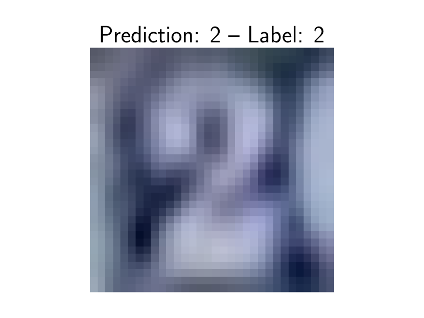
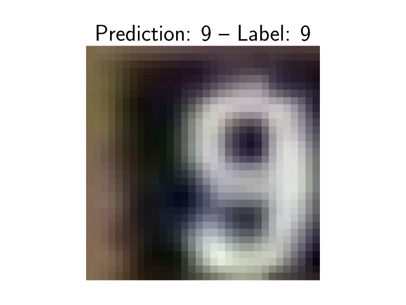
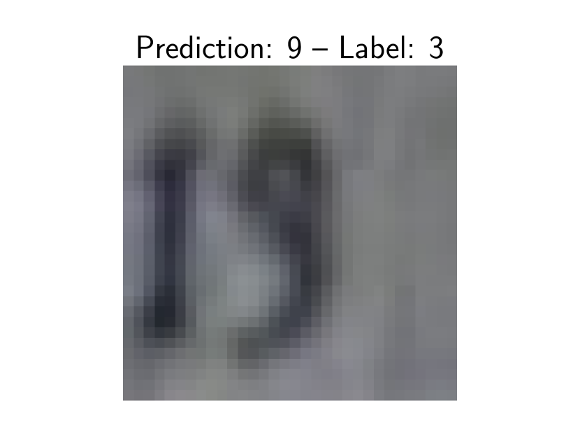
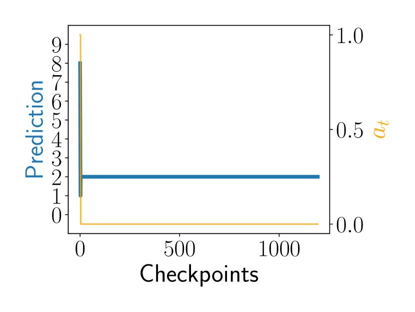
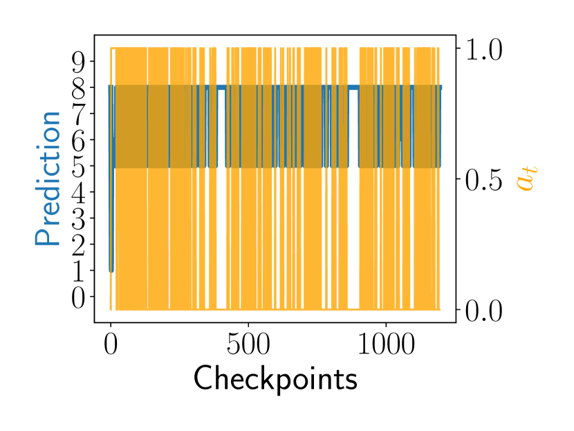
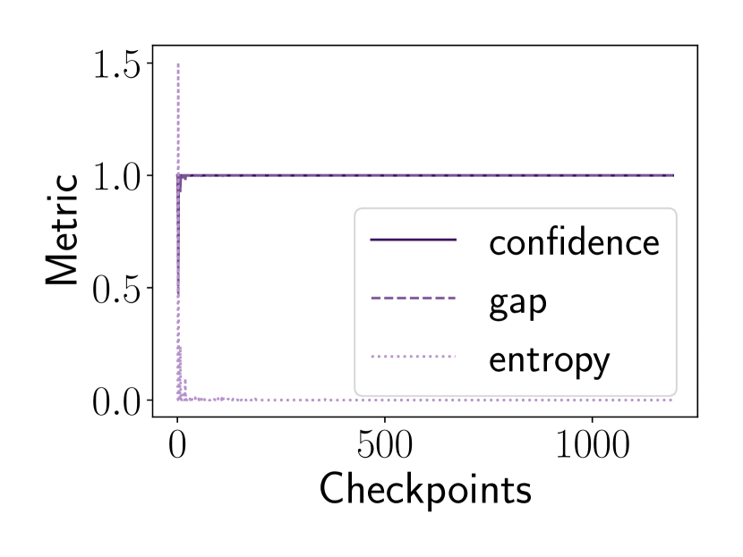
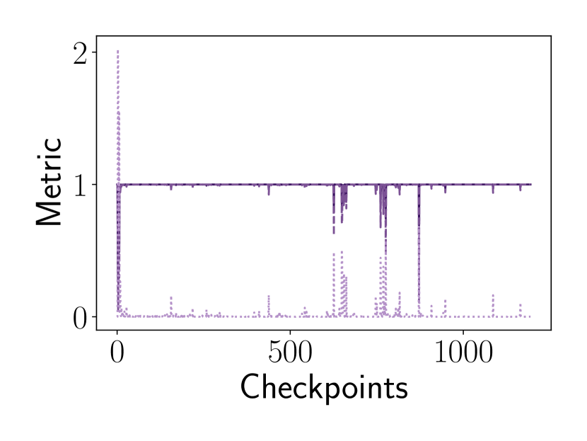
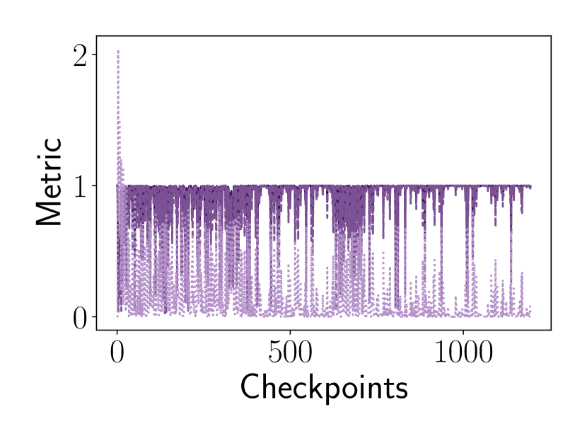
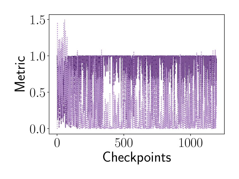
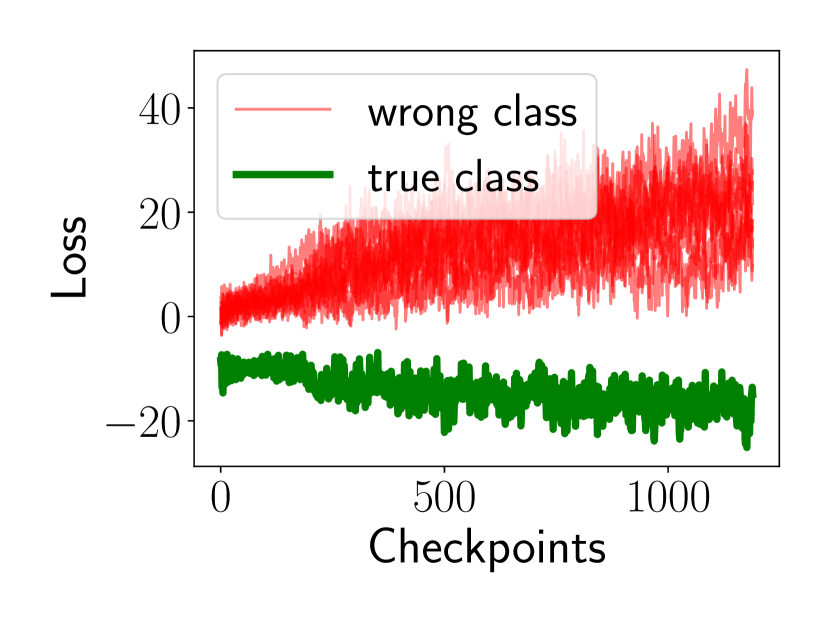
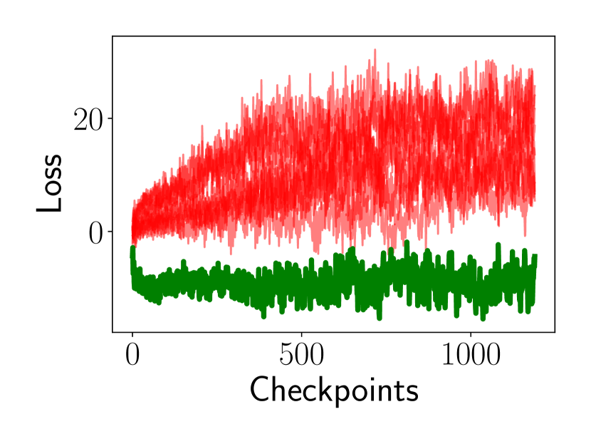
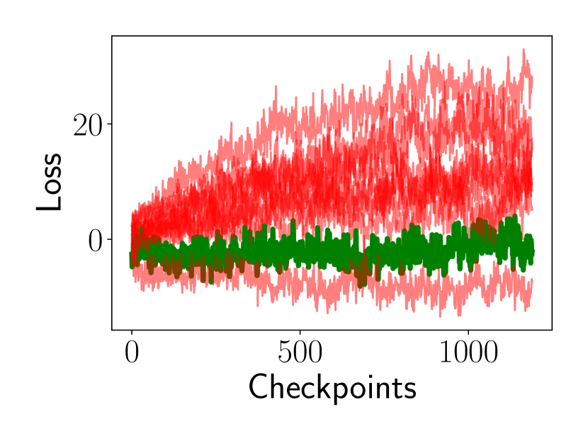
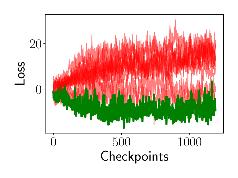
Figure 7: Individual SVHN examples. We extend Figure 2 by also including the evolution of the confidence, the gap, and the entropy over the course of training in the third row. In the final row, we further plot the loss evolution for all candidate classes. We note that the first two examples are easy to classify as indicated by mostly stationary metrics and a clear loss separation, while the last two examples are harder to classify since they exhibit highly erratic metrics and ambiguous loss curves.

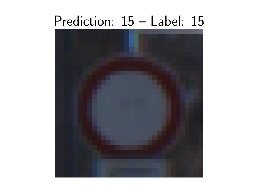
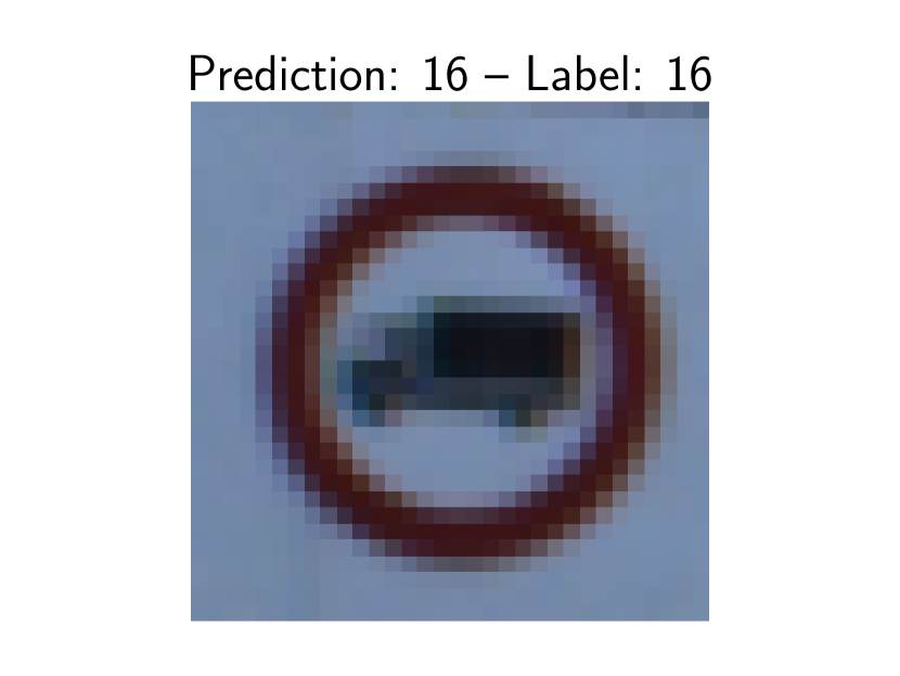
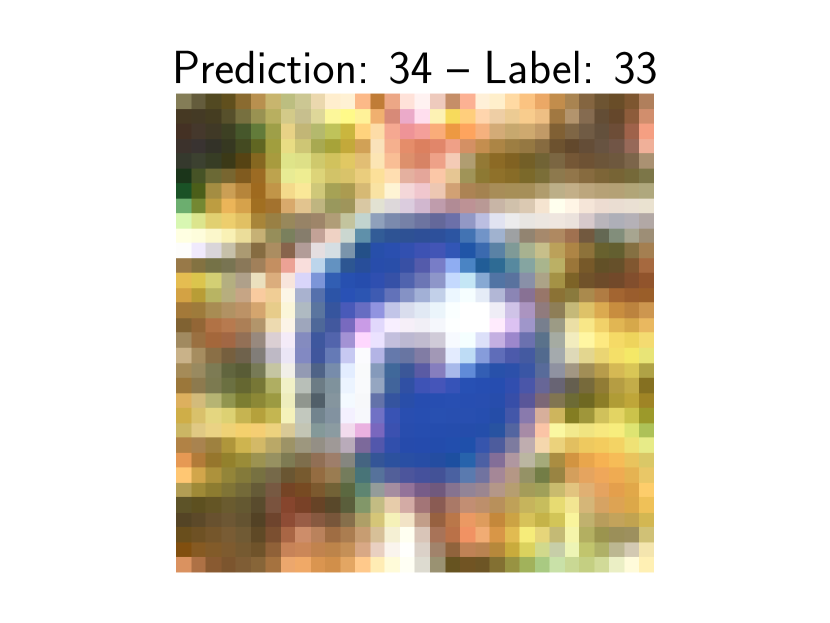
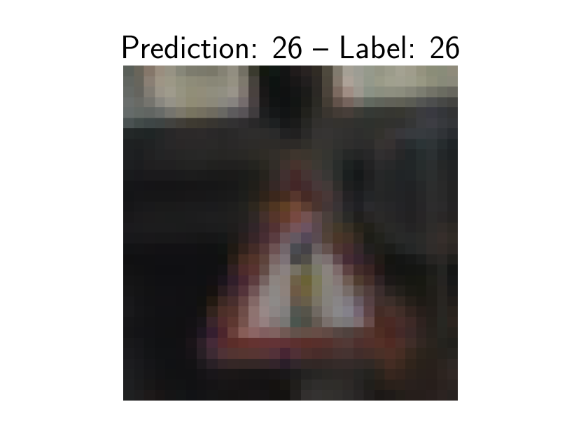
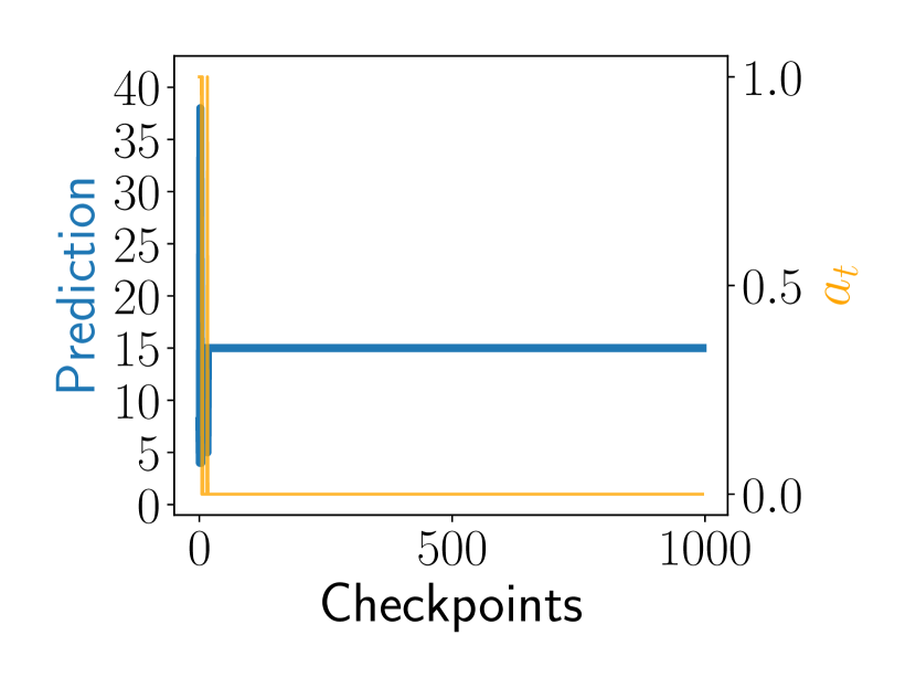
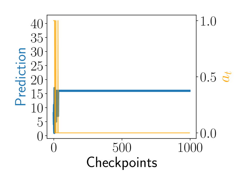
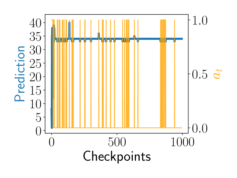
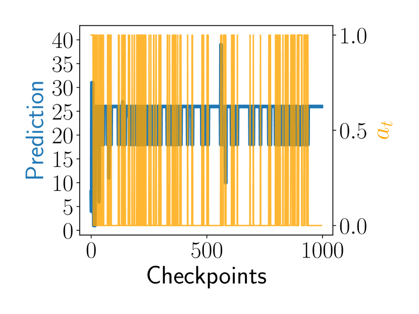
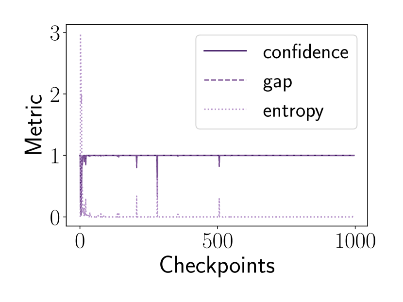
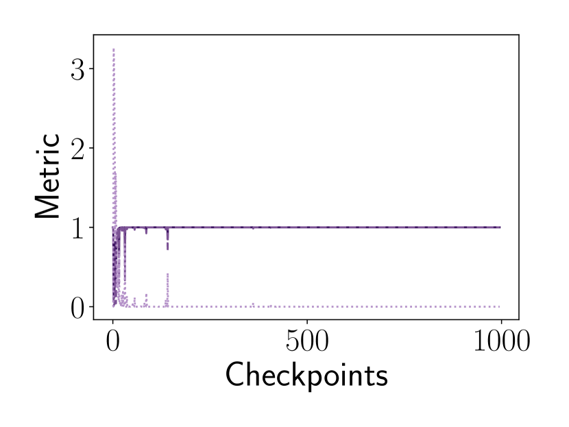
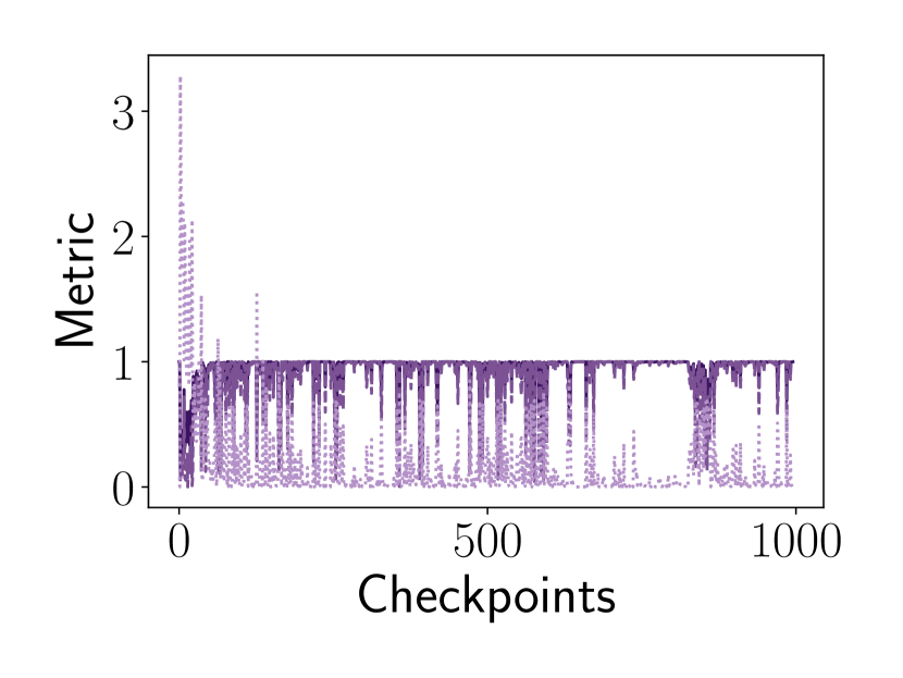
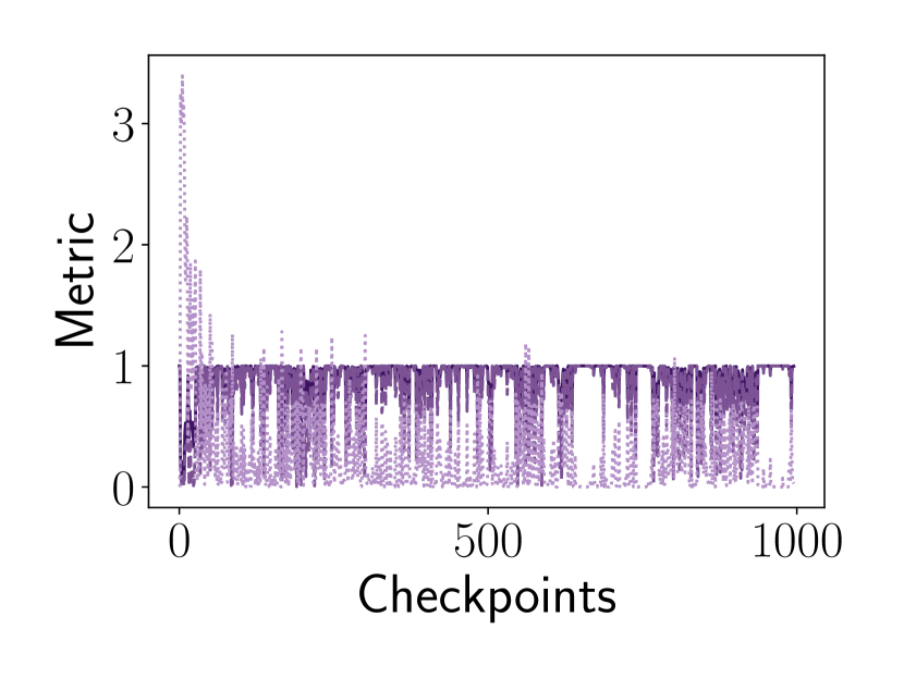
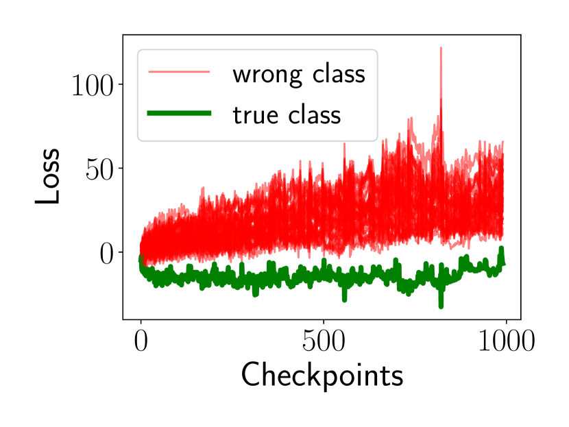
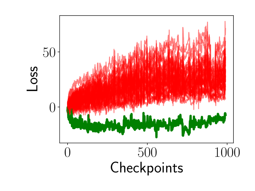
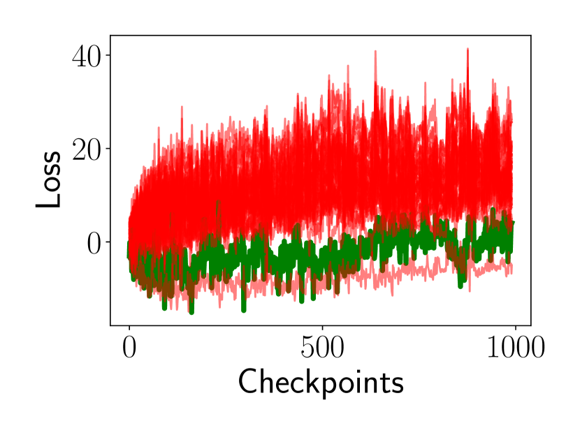
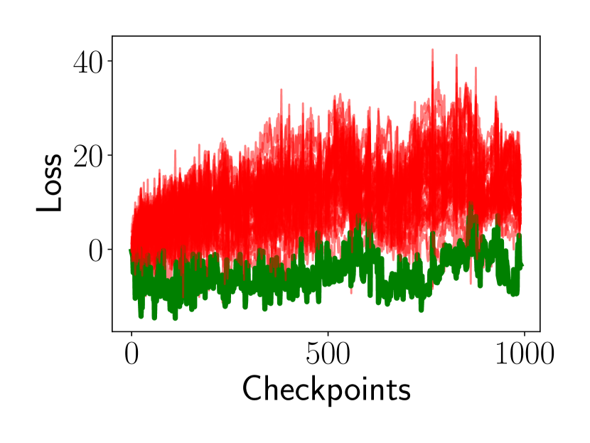
Figure 8: Individual GTSRB examples. Similar as Figure 7.

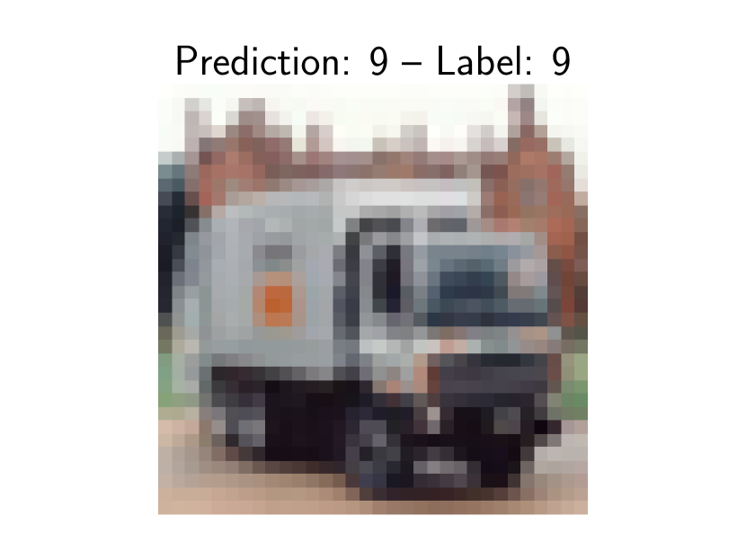
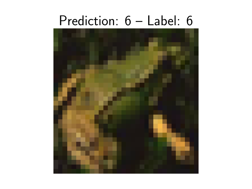
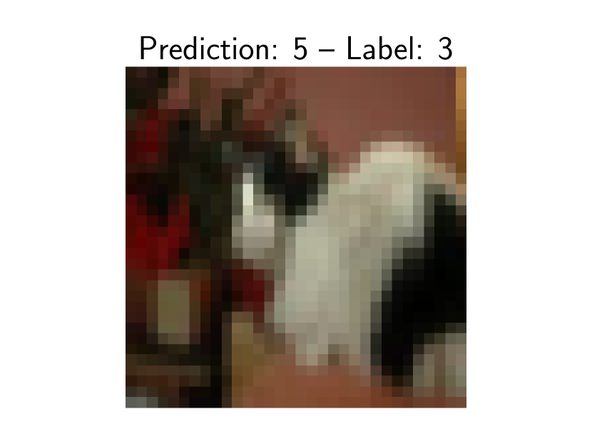
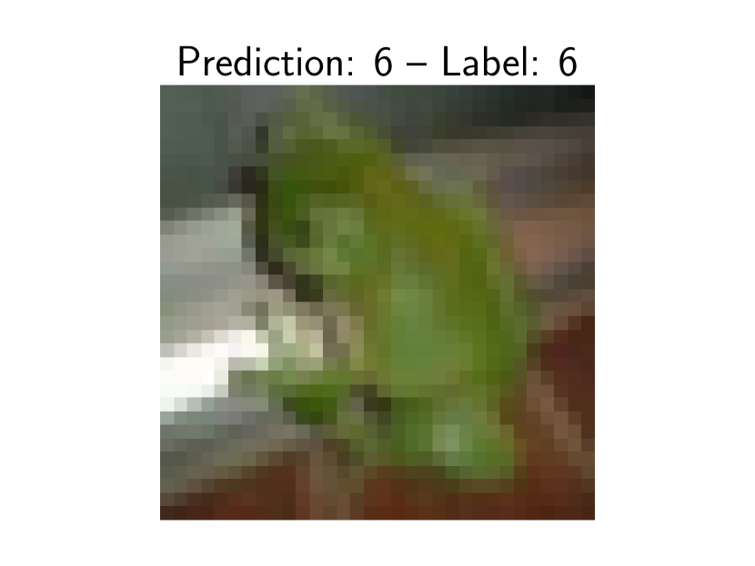
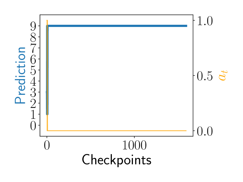
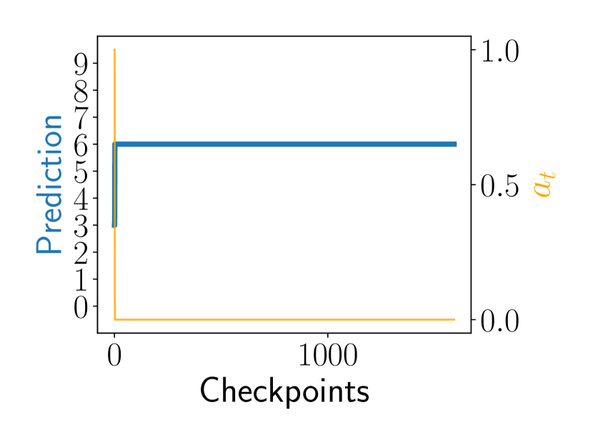
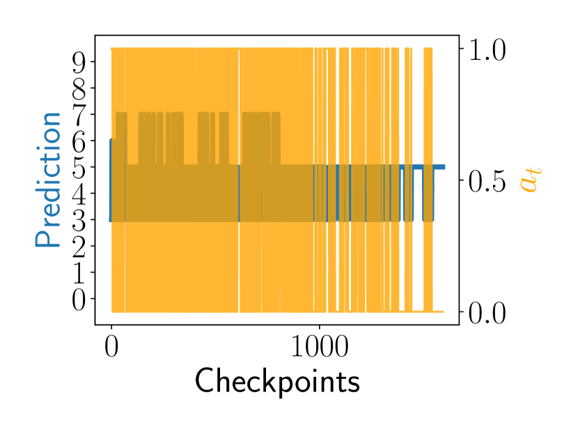
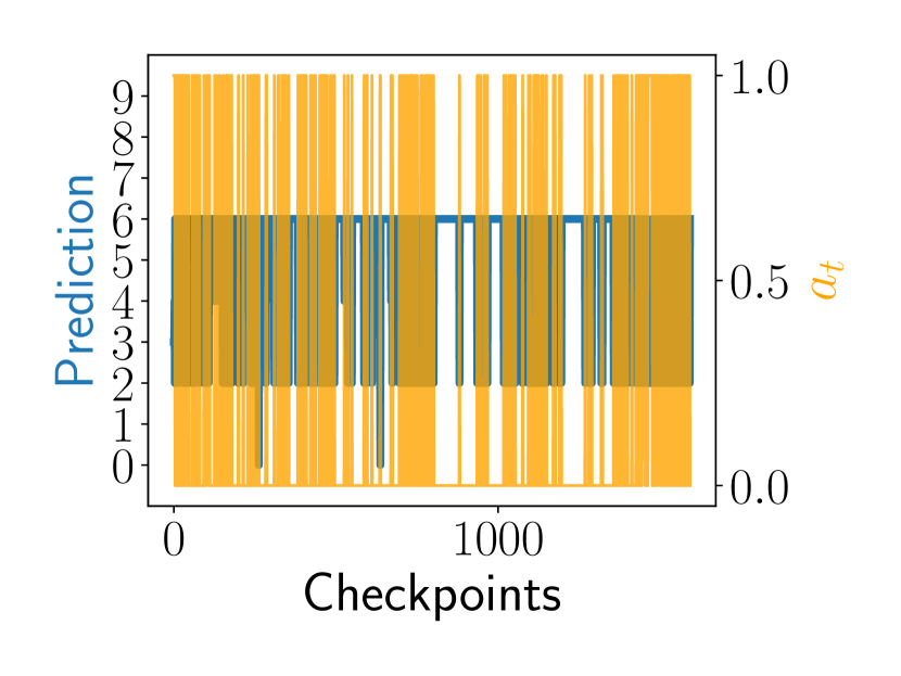
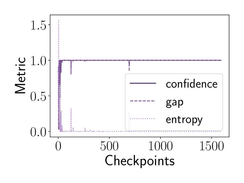
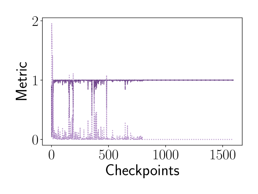
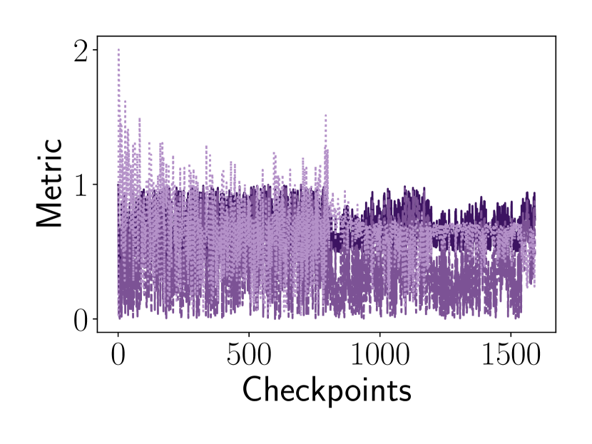
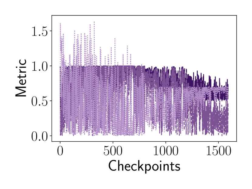
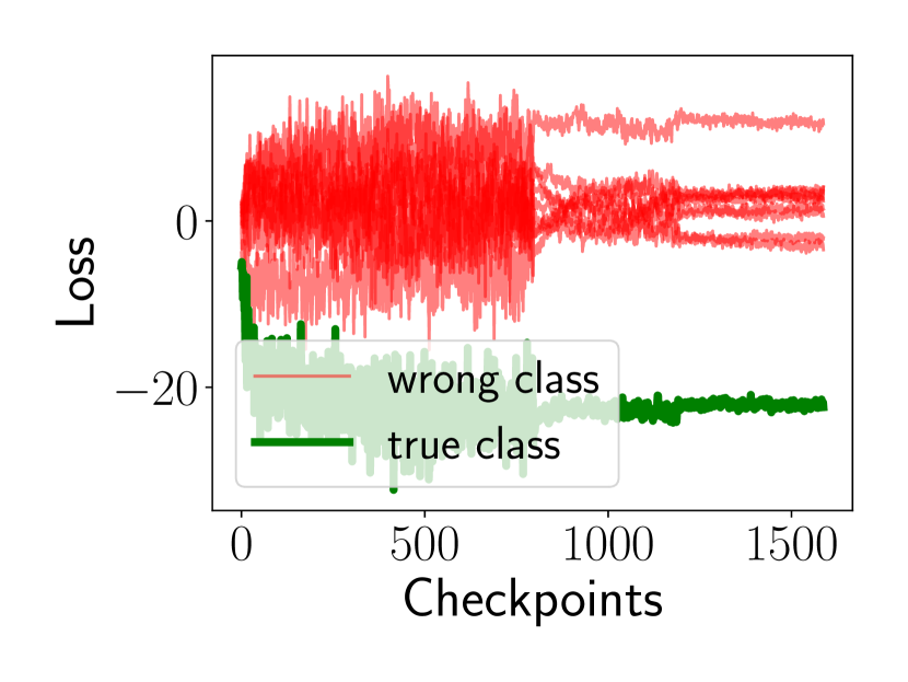
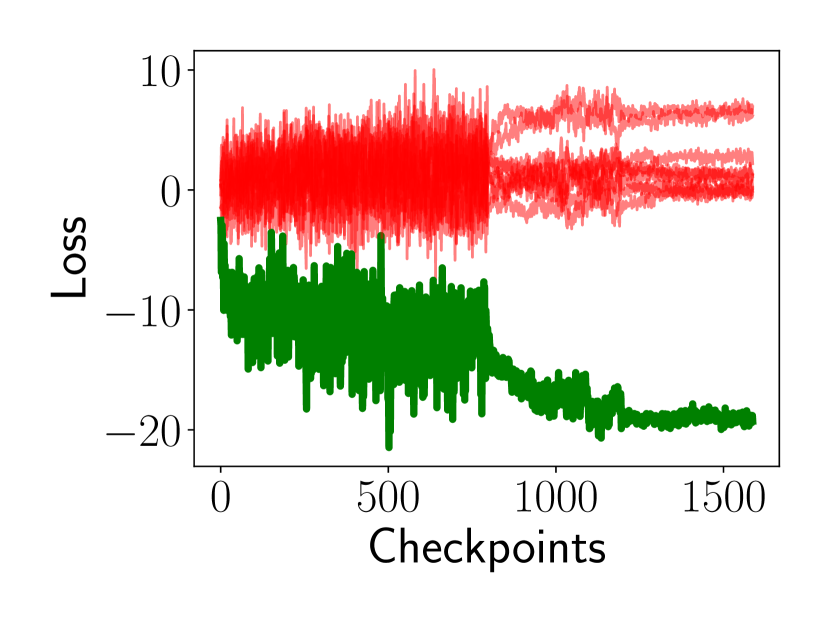
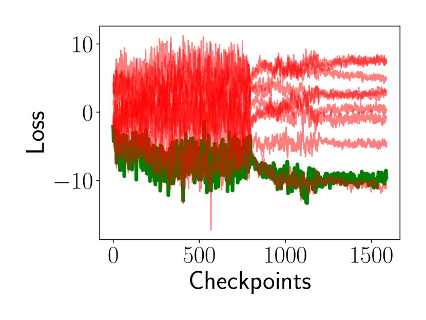
Figure 9: Individual CIFAR-10 examples. Similar as Figure 7.

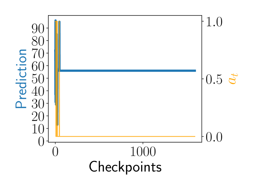
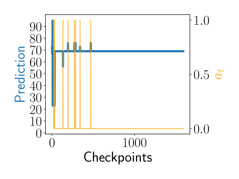
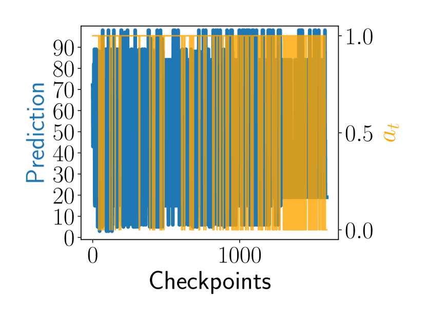
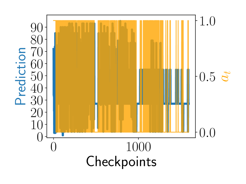
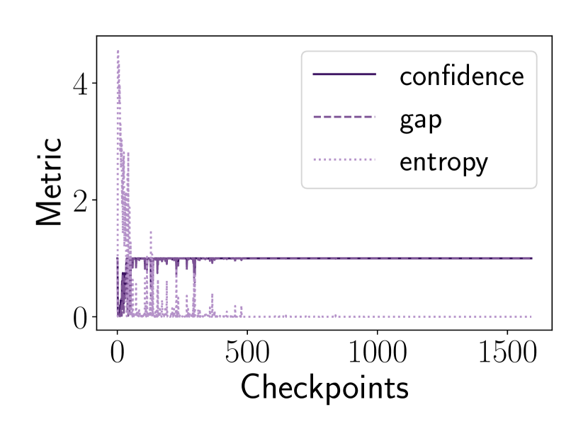
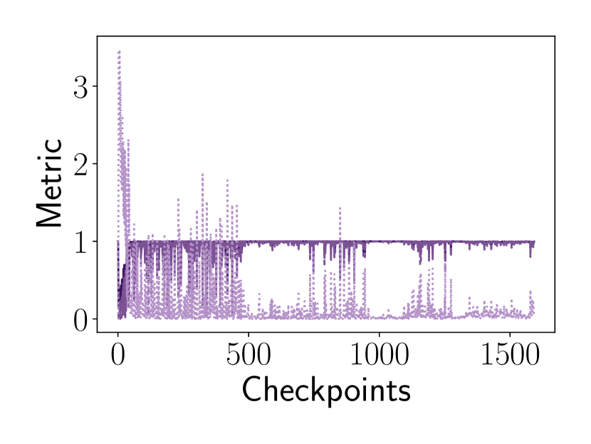
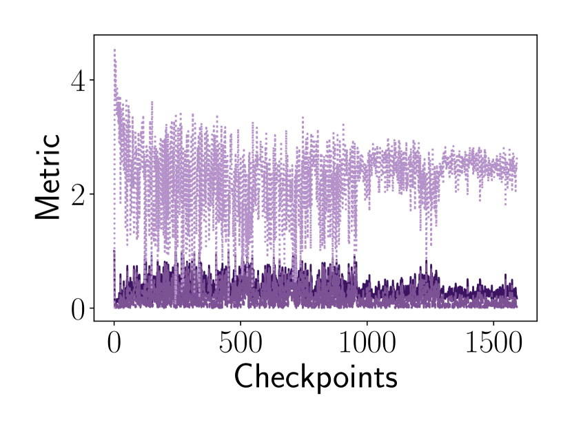
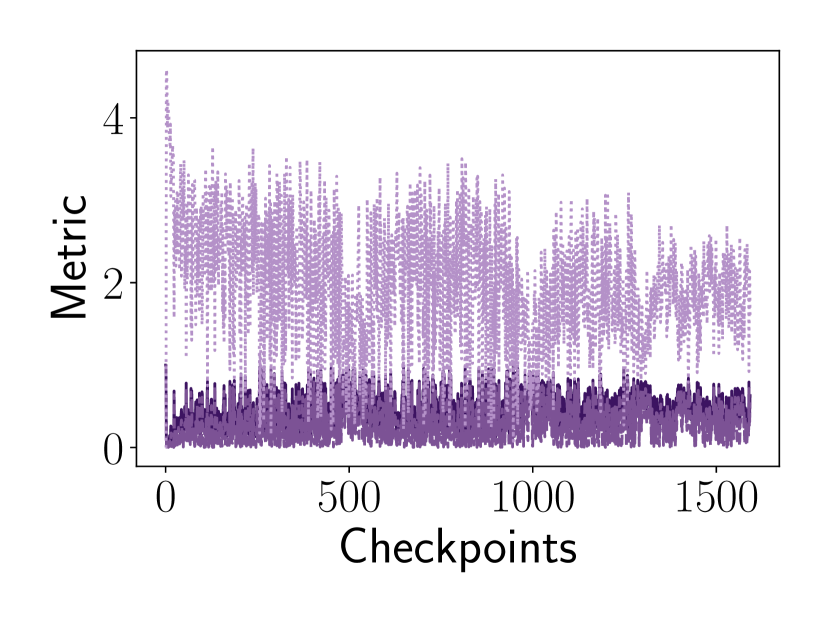
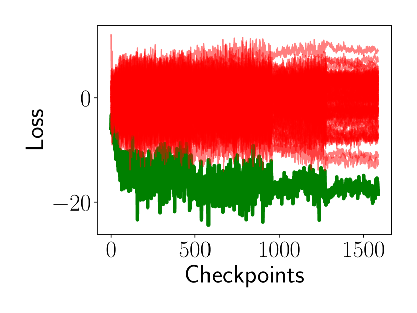
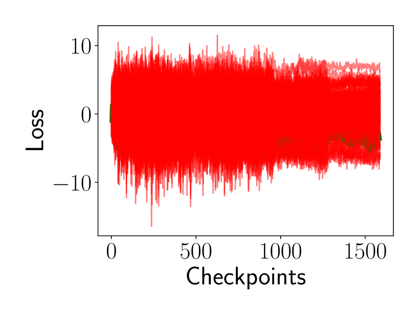
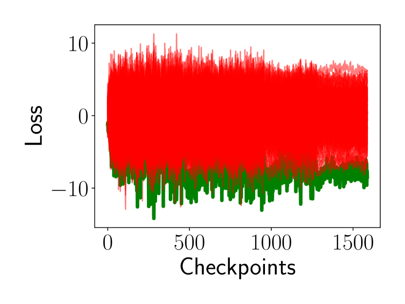
Figure 10: Individual CIFAR-100 examples. Similar as Figure 7.

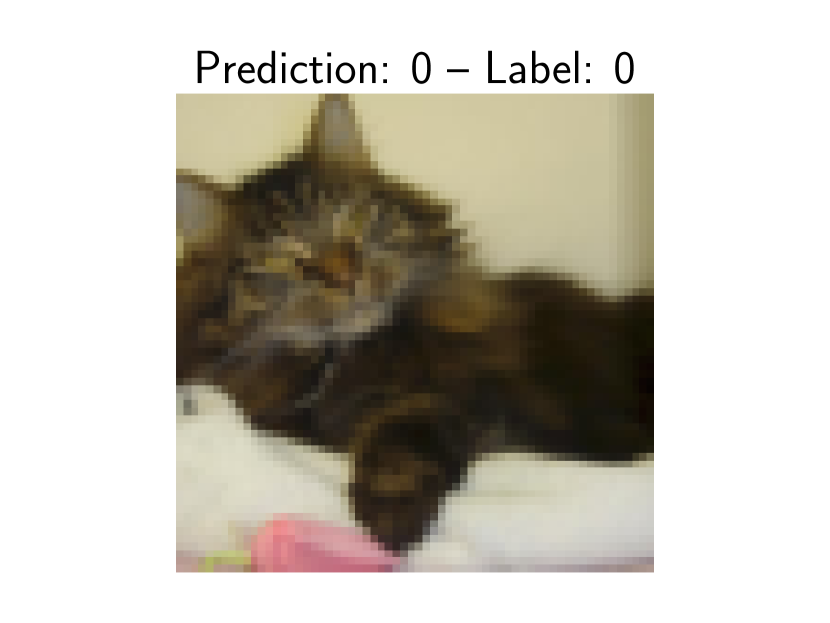
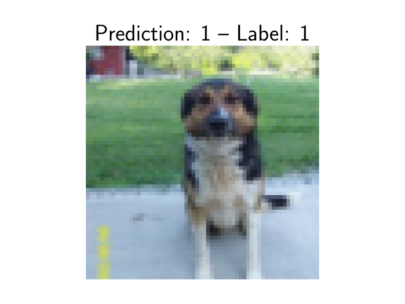
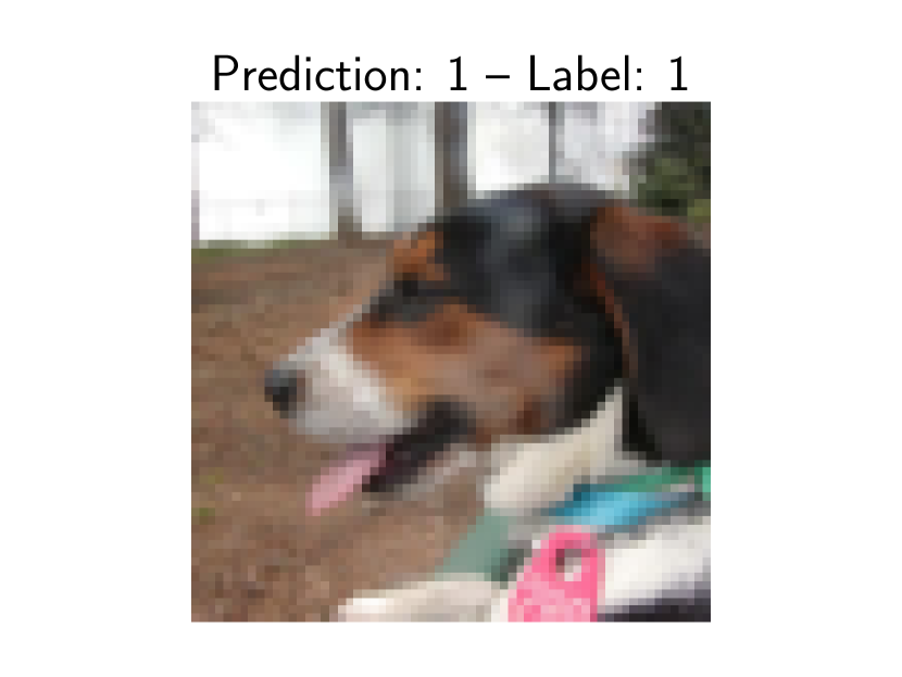
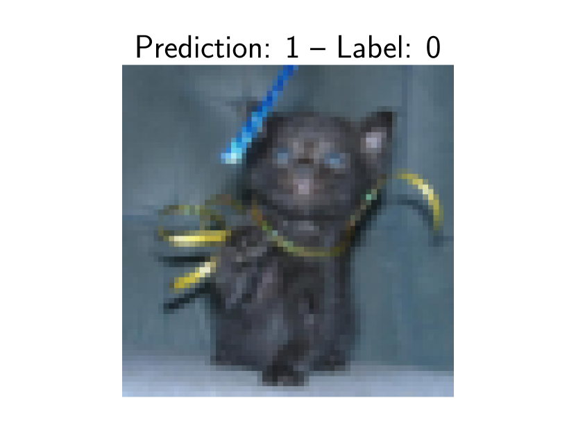
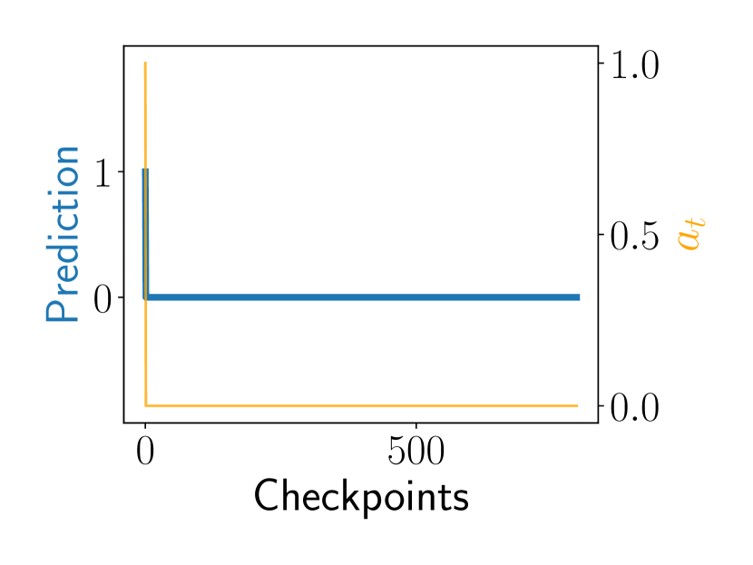
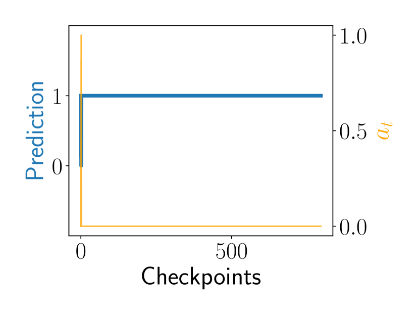
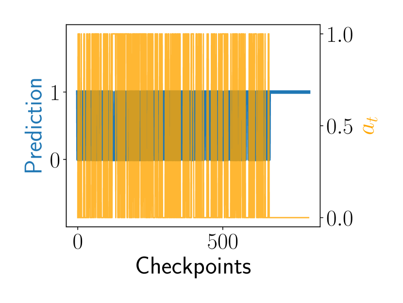
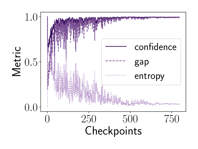
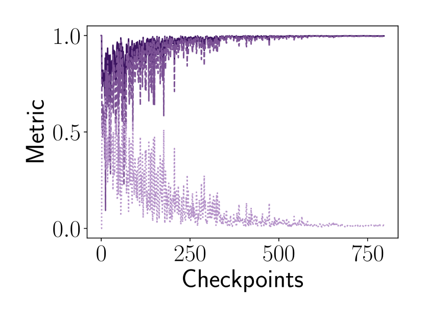
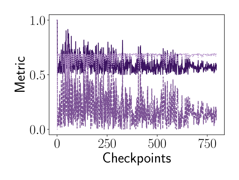
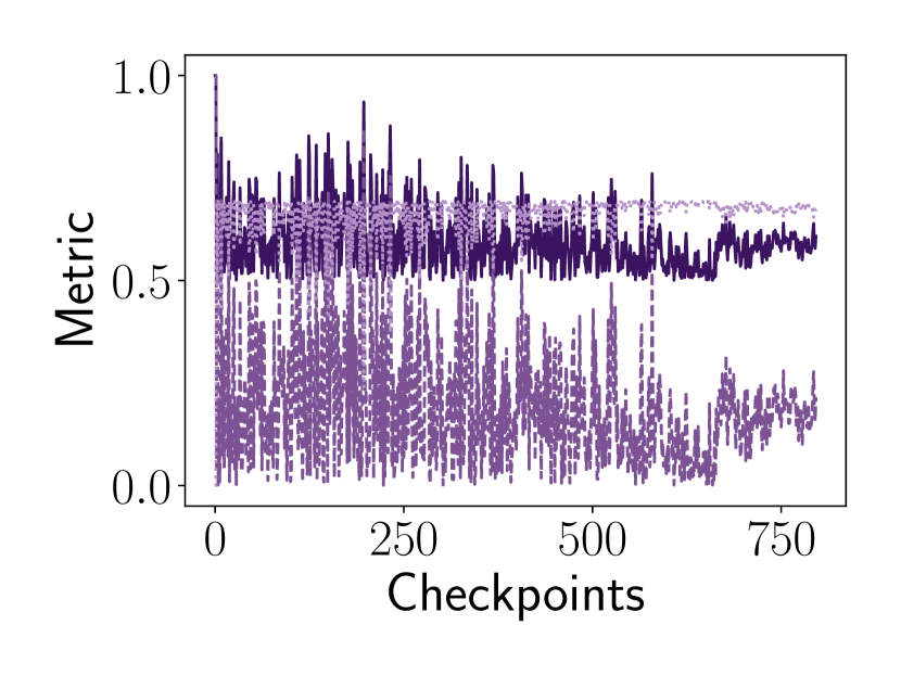
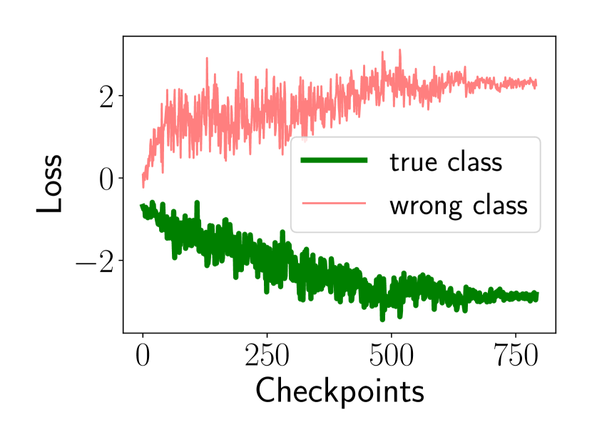
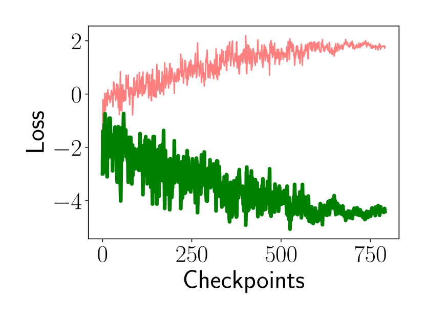
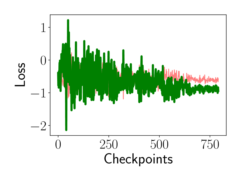
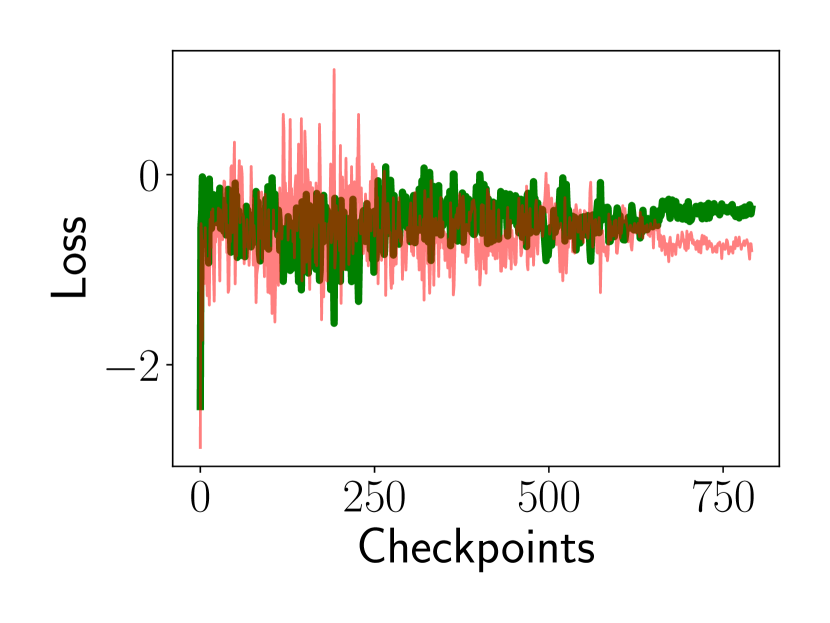
Figure 11: Individual Cats & Dogs examples. Similar as Figure 7.

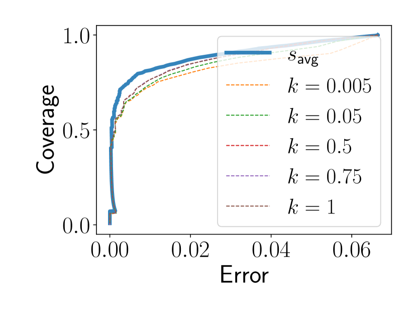
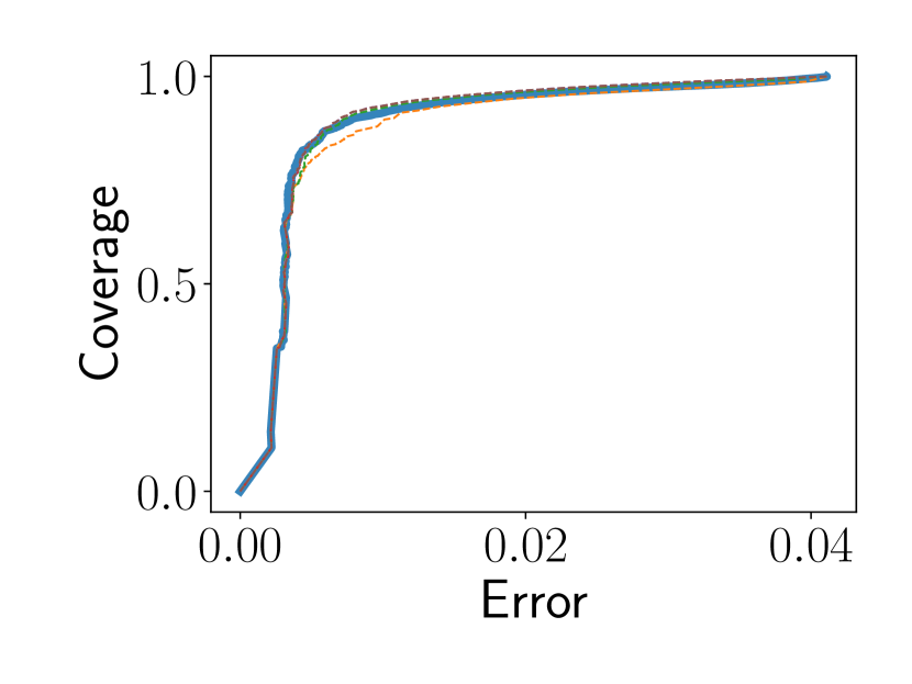
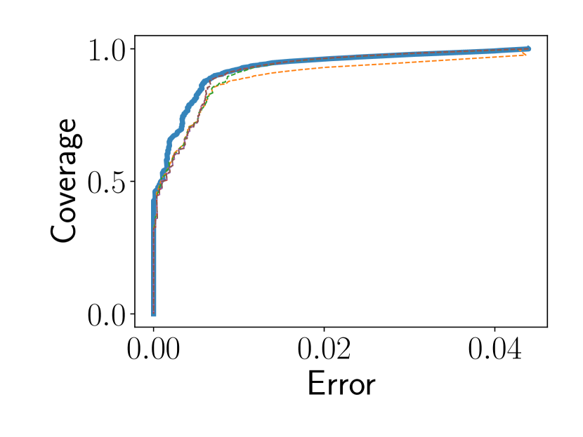
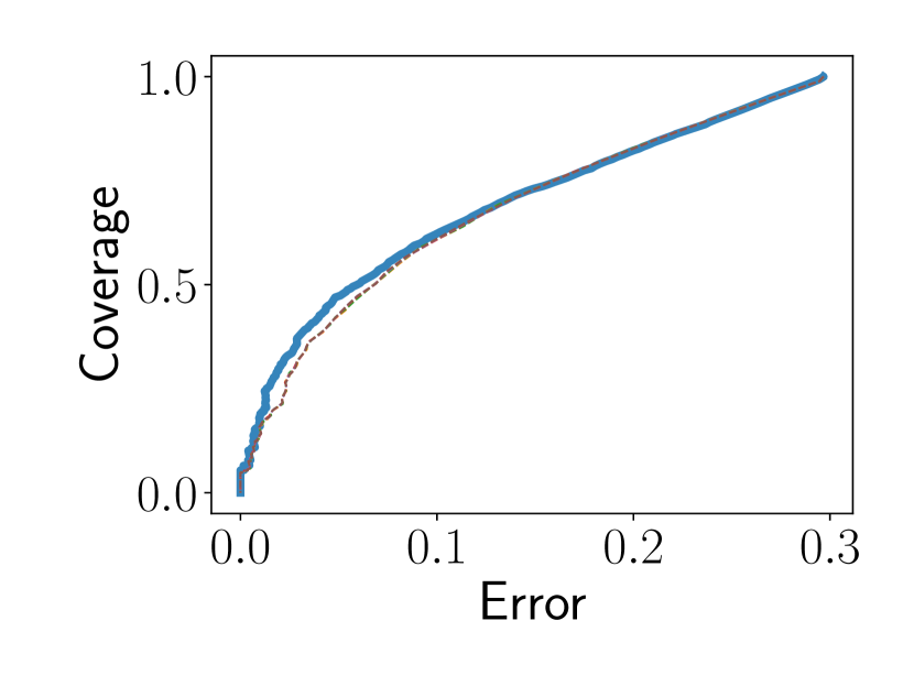
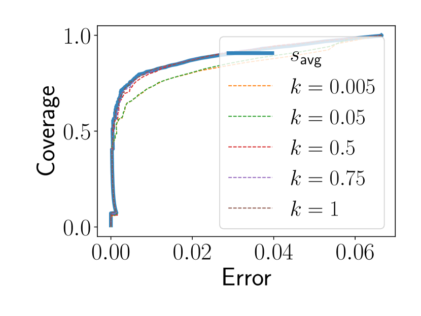
(a) CIFAR-10

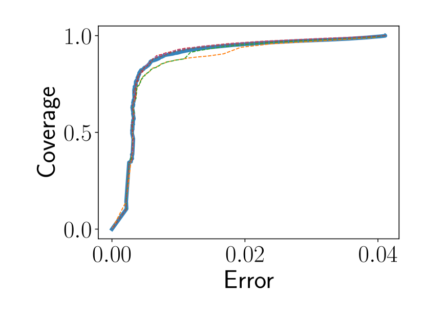
(b) SVHN

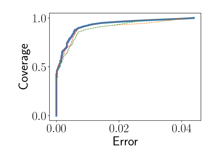
(c) GTSRB

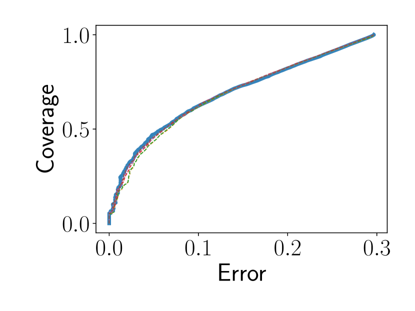
(d) CIFAR-100

Figure 12: Coverage/error trade-off when incorporating $e_{t}$ into $s_{\text{min}}$ and $s_{\text{avg}}$. In the first row, the solid blue line corresponds to NNTD$(s_{\text{avg}},0.05)$ while the dashed lines show the performance when we incorporate an empirical estimate of $e_{t}$ for various weightings $v_{i}$. In the second row, maintaining the solid blue line as NNTD$(s_{\text{avg}},0.05)$, we fix $v_{t}$ at $k=0.05$ and test various continuous approximations of $e_{t}$ as $e_{t}=1-t^{k}$ for $k\in(0,1]$. Overall, we find that introducing an adaptable $e_{t}$ does not further improve the performance of $s_{\text{min}}$ and $s_{\text{avg}}$ with $e_{t}=0$.

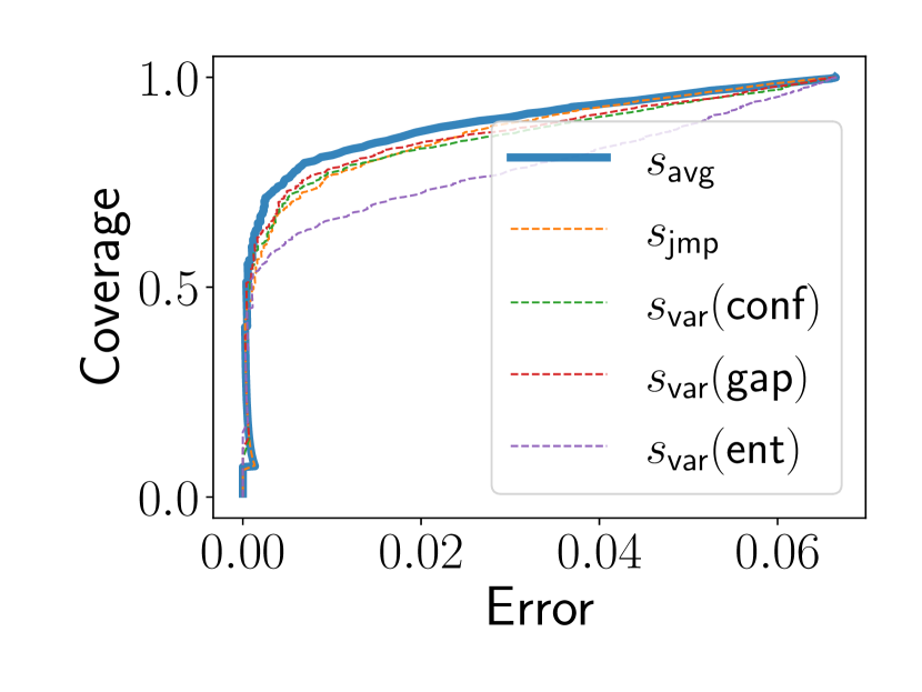
(a) CIFAR-10

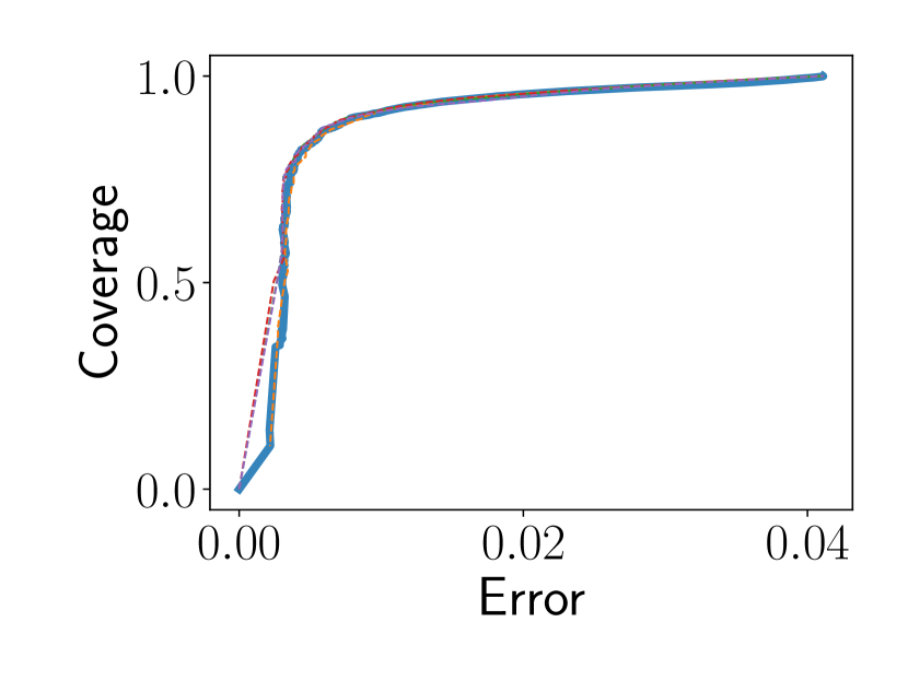
(b) SVHN

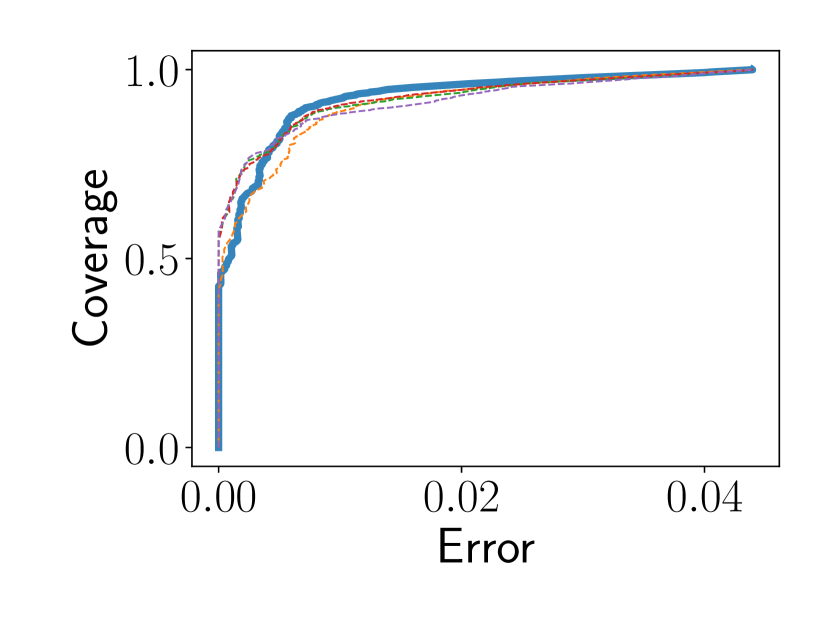
(c) GTSRB

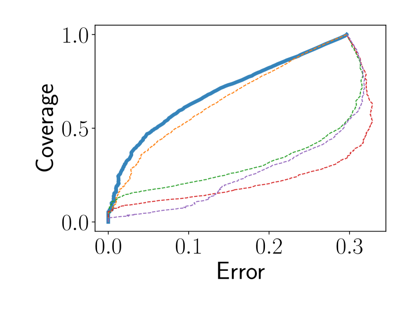
(d) CIFAR-100

Figure 13: Coverage/error trade-off of NNTD for alternate scores. We find that neither the jump score, nor any of the weighted variance metrics at their optimal $k$ for $v_{i}$ outperform NNTD$(s_{\text{avg}},0.05)$.

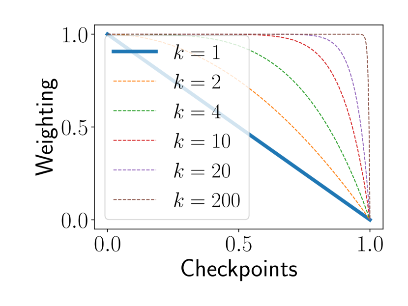
(a) Concave weighting

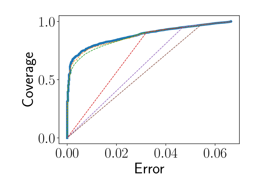
(b) CIFAR-10

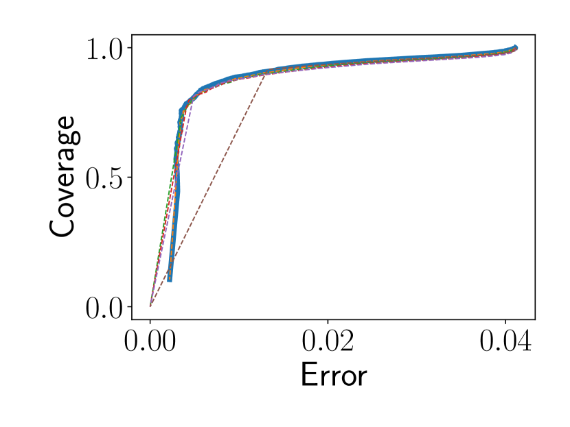
(c) SVHN

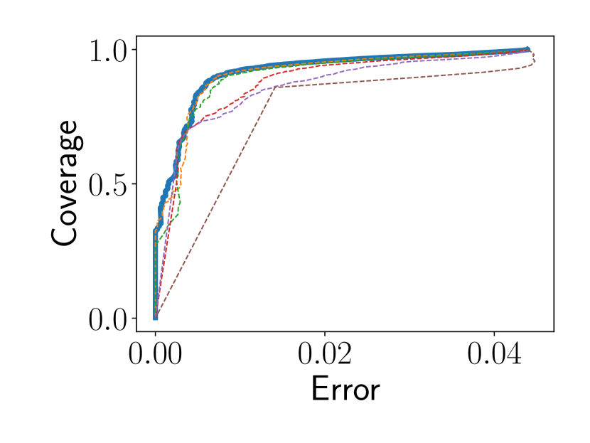
(d) GTSRB

Figure 14: Concave weighting used in $v_{t}=1-t^{k}$. Overall, since the best concave weighting is given by $k=1$, we conclude that no concave weighting outperforms any convex weighting.

Table 6: Coverage/Error trade-off of NNTD as a function of the accounted data points (CIFAR-10 left, SVHN right). We observe that large parts of the training process contain valuable sigals for selective classification.

Target Coverage	100%	90%	80%	50%	20%	10%
100%	6.07	6.08	6.10	6.15	6.18	6.20
95%	3.24	3.25	3.25	3.31	3.34	3.39
90%	1.83	1.83	1.84	1.88	1.91	1.93
80%	0.64	0.65	0.67	0.72	0.78	0.79
70%	0.34	0.34	0.36	0.38	0.40	0.40

Target Coverage	100%	90%	80%	50%	20%	10%
100%	2.68	2.70	2.73	2.83	2.88	2.92
95%	0.88	0.90	0.93	1.01	1.09	1.11
90%	0.55	0.57	0.59	0.62	0.68	0.73
80%	0.38	0.39	0.40	0.45	0.51	0.53
70%	0.33	0.33	0.35	0.41	0.44	0.45

Table 7: ImageNet coverage/error results. We observe that NNTD outperforms the SR baseline by a large margin and offers comparable performance as SAT.

Target	NNTD		SAT		SR
Error	Cov $\uparrow$	Err	Cov $\uparrow$	Err	Cov $\uparrow$	Err
10%	54.4	10.0	53.7	10.0	15.2	10.0
5%	26.3	5.0	25.8	5.0	5.4	5.0
2%	8.1	2.0	8.8	2.0	1.1	2.0
1%	3.6	1.0	4.0	1.8	0.7	1.8
0.5%	2.3	0.7	2.2	0.6	0.0	0.0

Target	NNTD		SAT		SR
Coverage	Cov	Err $\downarrow$	Cov	Err $\downarrow$	Cov	Err $\downarrow$
100%	100	24.2	100	24.2	100	24.2
95%	95.0	23.2	95.0	22.8	95.0	23.5
90%	90.0	22.5	90.0	22.6	90.0	22.9
80%	80.0	18.0	80.0	18.4	80.0	21.7
70%	70.0	14.1	70.0	14.3	70.0	20.7

Table 8: Performance of NNTD in comparison with OOD scores. We find that NNTD significantly outperforms common OOD detection approaches for the purpose of selective classification.

Dataset	Target	NNTD		Energy		Mahalanobis		ODIN
	Coverage	Cov	Err $\downarrow$	Cov	Err $\downarrow$	Cov	Err $\downarrow$	Cov	Err $\downarrow$
CIFAR-10	100%	100	6.07	100	6.07	100	6.07	100	6.07
	95%	95.0	3.24	95.0	3.99	95.0	4.44	95.1	6.04
	90%	90.1	1.83	90.0	2.67	90.0	2.93	88.9	6.01
	80%	79.9	0.64	80.0	1.10	80.1	1.20	88.9	6.01
	70%	69.8	0.34	70.0	0.83	69.9	0.82	68.3	4.41
SVHN	100%	100	2.68	100	2.68	100	2.68	100	2.68
	95%	95.0	0.88	95.1	1.35	95.1	1.51	95.0	2.67
	90%	90.1	0.55	89.9	0.92	90.0	1.04	89.9	2.64
	80%	79.9	0.38	79.9	0.70	80.3	0.70	81.9	2.51
	70%	69.8	0.33	70.0	0.58	69.8	0.58	74.9	2.18

Table 9: Performance at low target errors. Same results as in Table 1 but includes standard deviations.

Dataset	Target	NNTD		SAT		DG		SN		SR		MC-DO
	Error	Cov $\uparrow$	Err	Cov $\uparrow$	Err	Cov $\uparrow$	Err	Cov $\uparrow$	Err	Cov $\uparrow$	Err	Cov $\uparrow$	Err
CIFAR-10	2%	91.2 ($\pm$ 0.05)	1.99 ($\pm$ 0.01)	90.3 ($\pm$ 0.03)	1.97 ($\pm$ 0.02)	89.1 ($\pm$ 0.04)	2.02 ($\pm$ 0.01)	88.3 ($\pm$ 0.03)	2.03 ($\pm$ 0.02)	85.8 ($\pm$ 0.08)	1.98 ($\pm$ 0.02)	86.1 ($\pm$ 0.07)	2.01 ($\pm$ 0.01)
	1%	86.4 ($\pm$ 0.03)	1.00 ($\pm$ 0.01)	86.1 ($\pm$ 0.02)	1.02 ($\pm$ 0.02)	85.5 ($\pm$ 0.07)	1.03 ($\pm$ 0.02)	84.4 ($\pm$ 0.06)	0.98 ($\pm$ 0.02)	79.1 ($\pm$ 0.08)	1.01 ($\pm$ 0.03)	79.9 ($\pm$ 0.08)	1.01 ($\pm$ 0.03)
	0.5%	75.9 ($\pm$ 0.04)	0.49 ($\pm$ 0.02)	76.0 ($\pm$ 0.05)	0.51 ($\pm$ 0.02)	75.2 ($\pm$ 0.08)	0.5 ($\pm$ 0.03)	74.7 ($\pm$ 0.09)	0.49 ($\pm$ 0.01)	71.2 ($\pm$ 0.05)	0.51 ($\pm$ 0.02)	72.0 ($\pm$ 0.03)	0.50 ($\pm$ 0.03)
SVHN	2%	98.5 ($\pm$ 0.05)	1.98 ($\pm$ 0.03)	98.2 ($\pm$ 0.04)	1.99 ($\pm$ 0.02)	97.8 ($\pm$ 0.03)	2.06 ($\pm$ 0.05)	97.7 ($\pm$ 0.06)	2.03 ($\pm$ 0.02)	97.6 ($\pm$ 0.05)	1.99 ($\pm$ 0.03)	97.9 ($\pm$ 0.03)	2.00 ($\pm$ 0.04)
	1%	96.3 ($\pm$ 0.03)	0.99 ($\pm$ 0.02)	95.7 ($\pm$ 0.02)	1.03 ($\pm$ 0.03)	94.8 ($\pm$ 0.04)	0.99 ($\pm$ 0.01)	94.5 ($\pm$ 0.03)	1.04 ($\pm$ 0.02)	93.5 ($\pm$ 0.05)	1.01 ($\pm$ 0.03)	94.1 ($\pm$ 0.06)	0.97 ($\pm$ 0.02)
	0.5%	88.1 ($\pm$ 0.02)	0.50 ($\pm$ 0.02)	87.9 ($\pm$ 0.05)	0.51 ($\pm$ 0.01)	86.4 ($\pm$ 0.04)	0.51 ($\pm$ 0.01)	86.0 ($\pm$ 0.04)	0.51 ($\pm$ 0.01)	70.0 ($\pm$ 0.09)	0.50 ($\pm$ 0.04)	70.1 ($\pm$ 0.04)	0.49 ($\pm$ 0.03)
Cats & Dogs	2%	97.7 ($\pm$ 0.09)	2.01 ($\pm$ 0.03)	98.2 ($\pm$ 0.02)	1.98 ($\pm$ 0.03)	98.0 ($\pm$ 0.05)	2.03 ($\pm$ 0.02)	97.4 ($\pm$ 0.05)	1.98 ($\pm$ 0.03)	95.1 ($\pm$ 0.12)	1.99 ($\pm$ 0.04)	95.7 ($\pm$ 0.10)	1.99 ($\pm$ 0.03)
	1%	93.1 ($\pm$ 0.03)	1.01 ($\pm$ 0.02)	93.6 ($\pm$ 0.02)	0.98 ($\pm$ 0.03)	92.6 ($\pm$ 0.08)	0.97 ($\pm$ 0.04)	92.2 ($\pm$ 0.05)	0.98 ($\pm$ 0.02)	86.9 ($\pm$ 0.13)	0.98 ($\pm$ 0.04)	88.6 ($\pm$ 0.09)	1.01 ($\pm$ 0.02)
	0.5%	85.7 ($\pm$ 0.06)	0.51 ($\pm$ 0.02)	86.0 ($\pm$ 0.04)	0.49 ($\pm$ 0.01)	85.3 ($\pm$ 0.02)	0.49 ($\pm$ 0.02)	84.8 ($\pm$ 0.03)	0.46 ($\pm$ 0.05)	68.4 ($\pm$ 0.10)	0.48 ($\pm$ 0.02)	70.1 ($\pm$ 0.08)	0.51 ($\pm$ 0.03)

Table 10: Performance at high target coverage. Same results as in Table 2 but includes standard deviations.

Dataset	Target	NNTD		SAT		DG		SN		SR		MC-DO
	Coverage	Cov	Err $\downarrow$	Cov	Err $\downarrow$	Cov	Err $\downarrow$	Cov	Err $\downarrow$	Cov	Err $\downarrow$	Cov	Err $\downarrow$
CIFAR-10	100%	100 ($\pm$ 0.00)	6.07 ($\pm$ 0.05)	100 ($\pm$ 0.00)	6.06 ($\pm$ 0.03)	100 ($\pm$ 0.00)	6.11 ($\pm$ 0.05)	100 ($\pm$ 0.00)	6.13 ($\pm$ 0.03)	100 ($\pm$ 0.00)	6.07 ($\pm$ 0.05)	100 ($\pm$ 0.00)	6.07 ($\pm$ 0.05)
	95%	95.0 ($\pm$ 0.01)	3.24 ($\pm$ 0.03)	95.1 ($\pm$ 0.01)	3.32 ($\pm$ 0.05)	95.1 ($\pm$ 0.02)	3.47 ($\pm$ 0.06)	95.0 ($\pm$ 0.01)	4.08 ($\pm$ 0.08)	94.9 ($\pm$ 0.03)	4.48 ($\pm$ 0.07)	95.1 ($\pm$ 0.04)	4.48 ($\pm$ 0.09)
	90%	90.1 ($\pm$ 0.02)	1.83 ($\pm$ 0.04)	89.9 ($\pm$ 0.02)	1.90 ($\pm$ 0.02)	90.0 ($\pm$ 0.01)	2.19 ($\pm$ 0.05)	90.1 ($\pm$ 0.02)	2.29 ($\pm$ 0.03)	90.1 ($\pm$ 0.02)	2.78 ($\pm$ 0.06)	90.0 ($\pm$ 0.02)	2.87 ($\pm$ 0.07)
	80%	79.9 ($\pm$ 0.02)	0.64 ($\pm$ 0.03)	80.0 ($\pm$ 0.00)	0.65 ($\pm$ 0.04)	80.1 ($\pm$ 0.03)	0.66 ($\pm$ 0.04)	80.1 ($\pm$ 0.01)	0.81 ($\pm$ 0.07)	79.8 ($\pm$ 0.02)	1.05 ($\pm$ 0.08)	79.9 ($\pm$ 0.01)	1.01 ($\pm$ 0.03)
	70%	69.8 ($\pm$ 0.03)	0.34 ($\pm$ 0.04)	69.9 ($\pm$ 0.03)	0.32 ($\pm$ 0.05)	69.8 ($\pm$ 0.04)	0.41 ($\pm$ 0.04)	70.2 ($\pm$ 0.03)	0.30 ($\pm$ 0.02)	70.0 ($\pm$ 0.01)	0.47 ($\pm$ 0.07)	70.1 ($\pm$ 0.02)	0.42 ($\pm$ 0.05)
SVHN	100%	100 ($\pm$ 0.00)	2.68 ($\pm$ 0.02)	100 ($\pm$ 0.00)	2.71 ($\pm$ 0.03)	100 ($\pm$ 0.00)	2.72 ($\pm$ 0.05)	100 ($\pm$ 0.00)	2.77 ($\pm$ 0.06)	100 ($\pm$ 0.00)	2.68 ($\pm$ 0.02)	100 ($\pm$ 0.00)	2.68 ($\pm$ 0.02)
	95%	95.0 ($\pm$ 0.01)	0.88 ($\pm$ 0.02)	95.1 ($\pm$ 0.02)	0.95 ($\pm$ 0.03)	95.1 ($\pm$ 0.01)	1.01 ($\pm$ 0.06)	95.0 ($\pm$ 0.02)	1.07 ($\pm$ 0.05)	94.9 ($\pm$ 0.03)	1.15 ($\pm$ 0.11)	95.1 ($\pm$ 0.02)	1.12 ($\pm$ 0.07)
	90%	90.1 ($\pm$ 0.02)	0.55 ($\pm$ 0.4)	89.9 ($\pm$ 0.01)	0.58 ($\pm$ 0.01)	90.0 ($\pm$ 0.00)	0.63 ($\pm$ 0.06)	90.1 ($\pm$ 0.01)	0.71 ($\pm$ 0.04)	90.1 ($\pm$ 0.02)	0.82 ($\pm$ 0.06)	90.0 ($\pm$ 0.02)	0.76 ($\pm$ 0.03)
	80%	79.9 ($\pm$ 0.01)	0.38 ($\pm$ 0.02)	80.0 ($\pm$ 0.01)	0.37 ($\pm$ 0.02)	80.1 ($\pm$ 0.01)	0.43 ($\pm$ 0.01)	80.1 ($\pm$ 0.00)	0.48 ($\pm$ 0.02)	79.8 ($\pm$ 0.03)	0.55 ($\pm$ 0.09)	79.9 ($\pm$ 0.02)	0.53 ($\pm$ 0.08)
	70%	69.8 ($\pm$ 0.03)	0.33 ($\pm$ 0.03)	69.9 ($\pm$ 0.02)	0.33 ($\pm$ 0.01)	69.8 ($\pm$ 0.04)	0.35 ($\pm$ 0.02)	70.2 ($\pm$ 0.02)	0.45 ($\pm$ 0.06)	70.0 ($\pm$ 0.01)	0.50 ($\pm$ 0.05)	70.1 ($\pm$ 0.02)	0.49 ($\pm$ 0.06)
Cats & Dogs	100%	100 ($\pm$ 0.00)	3.48 ($\pm$ 0.01)	100 ($\pm$ 0.00)	3.45 ($\pm$ 0.01)	100 ($\pm$ 0.00)	3.41 ($\pm$ 0.03)	100 ($\pm$ 0.00)	3.56 ($\pm$ 0.04)	100 ($\pm$ 0.00)	3.48 ($\pm$ 0.01)	100 ($\pm$ 0.00)	3.48 ($\pm$ 0.01)
	95%	95.1 ($\pm$ 0.02)	1.51 ($\pm$ 0.03)	95.1 ($\pm$ 0.03)	1.45 ($\pm$ 0.02)	95.0 ($\pm$ 0.01)	1.43 ($\pm$ 0.02)	94.9 ($\pm$ 0.02)	1.61 ($\pm$ 0.05)	94.8 ($\pm$ 0.03)	1.92 ($\pm$ 0.12)	95.1 ($\pm$ 0.02)	1.95 ($\pm$ 0.08)
	90%	90.1 ($\pm$ 0.03)	0.60 ($\pm$ 0.03)	89.9 ($\pm$ 0.02)	0.57 ($\pm$ 0.03)	90.0 ($\pm$ 0.01)	0.69 ($\pm$ 0.04)	90.1 ($\pm$ 0.02)	0.95 ($\pm$ 0.11)	90.1 ($\pm$ 0.03)	1.13 ($\pm$ 0.07)	90.0 ($\pm$ 0.01)	1.09 ($\pm$ 0.06)
	80%	79.9 ($\pm$ 0.01)	0.42 ($\pm$ 0.04)	80.0 ($\pm$ 0.01)	0.41 ($\pm$ 0.03)	80.1 ($\pm$ 0.02)	0.56 ($\pm$ 0.02)	80.1 ($\pm$ 0.03)	0.39 ($\pm$ 0.05)	79.8 ($\pm$ 0.02)	0.69 ($\pm$ 0.07)	79.9 ($\pm$ 0.02)	0.58 ($\pm$ 0.05)
	70%	69.8 ($\pm$ 0.02)	0.36 ($\pm$ 0.05)	69.9 ($\pm$ 0.03)	0.33 ($\pm$ 0.03)	69.8 ($\pm$ 0.03)	0.45 ($\pm$ 0.05)	70.2 ($\pm$ 0.03)	0.33 ($\pm$ 0.03)	70.0 ($\pm$ 0.01)	0.62 ($\pm$ 0.06)	70.1 ($\pm$ 0.02)	0.51 ($\pm$ 0.04)

References

- Agarwal et al. (2020) Chirag Agarwal, Daniel D’souza, and Sara Hooker. Estimating example difficulty using variance of gradients. arXiv preprint arXiv:2008.11600, 2020.
- Baldock et al. (2021) Robert Baldock, Hartmut Maennel, and Behnam Neyshabur. Deep learning through the lens of example difficulty. Advances in Neural Information Processing Systems, 34, 2021.
- Bassily et al. (2020) Raef Bassily, Vitaly Feldman, Cristóbal Guzmán, and Kunal Talwar. Stability of stochastic gradient descent on nonsmooth convex losses. Advances in Neural Information Processing Systems, 33:4381–4391, 2020.
- Challen et al. (2019) Robert Challen, Joshua Denny, Martin Pitt, Luke Gompels, Tom Edwards, and Krasimira Tsaneva-Atanasova. Artificial intelligence, bias and clinical safety. BMJ Quality & Safety, 28(3):231–237, 2019.
- Chang et al. (2017) Haw-Shiuan Chang, Erik Learned-Miller, and Andrew McCallum. Active bias: Training more accurate neural networks by emphasizing high variance samples. Advances in Neural Information Processing Systems, 30, 2017.
- El-Yaniv and Wiener (2010) Ran El-Yaniv and Yair Wiener. On the foundations of noise-free selective classification. Journal of Machine Learning Research, 11(53):1605–1641, 2010. URL http://jmlr.org/papers/v11/el-yaniv10a.html.
- Feldman and Zhang (2020) Vitaly Feldman and Chiyuan Zhang. What neural networks memorize and why: Discovering the long tail via influence estimation. Advances in Neural Information Processing Systems, 33:2881–2891, 2020.
- Feng et al. (2021) Jean Feng, Arjun Sondhi, Jessica Perry, and Noah Simon. Selective prediction-set models with coverage rate guarantees. Biometrics, 2021.
- Gal and Ghahramani (2016) Yarin Gal and Zoubin Ghahramani. Dropout as a bayesian approximation: Representing model uncertainty in deep learning. In international conference on machine learning, pages 1050–1059. PMLR, 2016.
- Gangrade et al. (2021) Aditya Gangrade, Anil Kag, and Venkatesh Saligrama. Selective classification via one-sided prediction. In International Conference on Artificial Intelligence and Statistics, pages 2179–2187. PMLR, 2021.
- Geifman and El-Yaniv (2017) Yonatan Geifman and Ran El-Yaniv. Selective classification for deep neural networks. Advances in neural information processing systems, 30, 2017.
- Geifman and El-Yaniv (2019) Yonatan Geifman and Ran El-Yaniv. Selectivenet: A deep neural network with an integrated reject option. In International Conference on Machine Learning, pages 2151–2159. PMLR, 2019.
- Geifman et al. (2018) Yonatan Geifman, Guy Uziel, and Ran El-Yaniv. Bias-reduced uncertainty estimation for deep neural classifiers. arXiv preprint arXiv:1805.08206, 2018.
- Ghodsi et al. (2021) Zahra Ghodsi, Siva Kumar Sastry Hari, Iuri Frosio, Timothy Tsai, Alejandro Troccoli, Stephen W Keckler, Siddharth Garg, and Anima Anandkumar. Generating and characterizing scenarios for safety testing of autonomous vehicles. arXiv preprint arXiv:2103.07403, 2021.
- Guo et al. (2017) Chuan Guo, Geoff Pleiss, Yu Sun, and Kilian Q Weinberger. On calibration of modern neural networks. In International Conference on Machine Learning, pages 1321–1330. PMLR, 2017.
- Hardt et al. (2016) Moritz Hardt, Ben Recht, and Yoram Singer. Train faster, generalize better: Stability of stochastic gradient descent. In International conference on machine learning, pages 1225–1234. PMLR, 2016.
- He et al. (2016) Kaiming He, Xiangyu Zhang, Shaoqing Ren, and Jian Sun. Deep residual learning for image recognition. In Proceedings of the IEEE conference on computer vision and pattern recognition, pages 770–778, 2016.
- Hooker et al. (2019) Sara Hooker, Aaron Courville, Gregory Clark, Yann Dauphin, and Andrea Frome. What do compressed deep neural networks forget? arXiv preprint arXiv:1911.05248, 2019.
- Houben et al. (2013) Sebastian Houben, Johannes Stallkamp, Jan Salmen, Marc Schlipsing, and Christian Igel. Detection of traffic signs in real-world images: The German Traffic Sign Detection Benchmark. In International Joint Conference on Neural Networks, number 1288, 2013.
- Huang et al. (2020) Lang Huang, Chao Zhang, and Hongyang Zhang. Self-adaptive training: beyond empirical risk minimization. Advances in neural information processing systems, 33:19365–19376, 2020.
- Jiang et al. (2020) Ziheng Jiang, Chiyuan Zhang, Kunal Talwar, and Michael C Mozer. Characterizing structural regularities of labeled data in overparameterized models. arXiv preprint arXiv:2002.03206, 2020.
- Jones et al. (2020) Erik Jones, Shiori Sagawa, Pang Wei Koh, Ananya Kumar, and Percy Liang. Selective classification can magnify disparities across groups. arXiv preprint arXiv:2010.14134, 2020.
- Khani et al. (2016) Fereshte Khani, Martin Rinard, and Percy Liang. Unanimous prediction for 100% precision with application to learning semantic mappings. arXiv preprint arXiv:1606.06368, 2016.
- Krizhevsky et al. (2009) Alex Krizhevsky, Geoffrey Hinton, et al. Learning multiple layers of features from tiny images. 2009.
- Lakshminarayanan et al. (2017) Balaji Lakshminarayanan, Alexander Pritzel, and Charles Blundell. Simple and scalable predictive uncertainty estimation using deep ensembles. In I. Guyon, U. Von Luxburg, S. Bengio, H. Wallach, R. Fergus, S. Vishwanathan, and R. Garnett, editors, Advances in Neural Information Processing Systems, volume 30. Curran Associates, Inc., 2017. URL https://proceedings.neurips.cc/paper/2017/file/9ef2ed4b7fd2c810847ffa5fa85bce38-Paper.pdf.
- Lee et al. (2018) Kimin Lee, Kibok Lee, Honglak Lee, and Jinwoo Shin. A simple unified framework for detecting out-of-distribution samples and adversarial attacks. Advances in neural information processing systems, 31, 2018.
- Liang et al. (2017) Shiyu Liang, Yixuan Li, and Rayadurgam Srikant. Enhancing the reliability of out-of-distribution image detection in neural networks. arXiv preprint arXiv:1706.02690, 2017.
- Liu et al. (2020) Weitang Liu, Xiaoyun Wang, John Owens, and Yixuan Li. Energy-based out-of-distribution detection. Advances in Neural Information Processing Systems, 33:21464–21475, 2020.
- Liu et al. (2019) Ziyin Liu, Zhikang Wang, Paul Pu Liang, Russ R Salakhutdinov, Louis-Philippe Morency, and Masahito Ueda. Deep gamblers: Learning to abstain with portfolio theory. Advances in Neural Information Processing Systems, 32, 2019.
- Mozannar and Sontag (2020) Hussein Mozannar and David Sontag. Consistent estimators for learning to defer to an expert. In International Conference on Machine Learning, pages 7076–7087. PMLR, 2020.
- Netzer et al. (2011) Yuval Netzer, Tao Wang, Adam Coates, Alessandro Bissacco, Bo Wu, and Andrew Y Ng. Reading digits in natural images with unsupervised feature learning. 2011.
- Schein and Ungar (2007) Andrew I Schein and Lyle H Ungar. Active learning for logistic regression: an evaluation. Machine Learning, 68(3):235–265, 2007.
- Simonyan and Zisserman (2014) Karen Simonyan and Andrew Zisserman. Very deep convolutional networks for large-scale image recognition. arXiv preprint arXiv:1409.1556, 2014.
- Thudi et al. (2022) Anvith Thudi, Hengrui Jia, Ilia Shumailov, and Nicolas Papernot. On the necessity of auditable algorithmic definitions for machine unlearning. In 31st USENIX Security Symposium (USENIX Security 22), pages 4007–4022, 2022.
- Toneva et al. (2018) Mariya Toneva, Alessandro Sordoni, Remi Tachet des Combes, Adam Trischler, Yoshua Bengio, and Geoffrey J Gordon. An empirical study of example forgetting during deep neural network learning. arXiv preprint arXiv:1812.05159, 2018.
- Vieira et al. (2021) Lucas Nunes Vieira, Minako O’Hagan, and Carol O’Sullivan. Understanding the societal impacts of machine translation: a critical review of the literature on medical and legal use cases. Information, Communication & Society, 24(11):1515–1532, 2021.