Casimir-Polder attraction and repulsion between nanoparticles and graphene in out-of-thermal-equilibrium conditions

Abstract

The nonequilibrium Casimir-Polder force between a nanoparticle and a graphene sheet kept at different temperatures is investigated in the framework of Dirac model using the formalism of the polarization tensor. It is shown that the force magnitude increases with increasing temperature of a graphene sheet. At larger separations an impact of nonequilibrium conditions on the force becomes smaller. According to our results, the attractive Casimir-Polder force vanishes at some definite nanoparticle-graphene separation and becomes repulsive at larger separations if the temperature of a graphene sheet is smaller than that of the environment. This effect may find applications both in fundamental investigations of graphene and for the control of forces in microdevices of bioelectronics.

I Introduction

The Casimir-Polder force 1 acts between two electrically neutral polarizable particles spaced at a distance far exceeding their sizes or experienced by the neutral polarizable particle which is well off a macroscopic interface. This is an attractive force caused by the combined action of the zero-point and thermal fluctuations of the electromagnetic field. In the condition of thermal equilibrium, i.e., under equal temperatures of the particles, material surface, and the environment, the Casimir-Polder free energy and force are expressed via the dynamic polarizability of these particles (atoms) and the reflection coefficients of electromagnetic fluctuations on the surface in the framework of the Lifshitz theory 2 ; 3 . The respective expressions follow from the Lifshitz formula for the Casimir force between two parallel plates when one of them is treated as a rarefied medium.

The obtained results found numerous applications in both fundamental and applied physics (see Refs. 4 ; 5 for a review). They were generalized 6 ; 7 ; 8 ; 9 ; 10 ; 11 for out-of-thermal-equilibrium conditions, e.g., for the case when the surface is kept at one temperature whereas a nanoparticle or an atom and the environment are characterized by some other temperature. Recently the Casimir force out of thermal equilibrium was considered for two similar plates with temperature-dependent dielectric permittivity 12 and for two superconducting plates 13 . The possibility of nonequilibrium repulsive Casimir force between two parallel plates was demonstrated in Ref. 14 .

The Casimir-Polder force between a nanoparticle and a flat surface is an important contribution to the total particle-surface interaction which includes also Born repulsion and mechanical contact forces 15 ; 16 . Investigation of interaction between nanoparticles and material surfaces is of great concern for designing sensing devices, such as electrochemical sensors and biosensors for the needs of bioelectronics 17 ; 18 ; 18a ; 18b . The out-of-thermal-equilibrium Casimir-Polder forces between a small sphere and a plate and between two small spheres were studies in Ref. 20a in the framework of general scattering formalism. It was shown that the force can be both attractive and repulsive and it turns into zero at some separations. It was also shown 19 that in out-of-thermal-equilibrium conditions a nanoparticle in the vicinity of a substrate made of nonreciprocal plasmonic material may even experience the lateral Casimir-Polder force.

During the last few years considerable study has been given to graphene which is an one-atom-thick sheet of carbon atoms possessing unusual properties 20 ; 21 ; 22 . The most important of them is that at energies below approximately 3 eV 23 the electronic quasiparticles in graphene are massless and are described by the relativistic Dirac equation, rather than by Schrödinger equation, where the speed of light $c$ is replaced with the Fermi velocity $v_{F}\approx c$/300. The Casimir-Polder interaction of different atoms with graphene in thermal equilibrium was studied in Refs. 24 ; 25 ; 26 ; 27 ; 29 ; 30 ; 31 ; 32 ; 33 ; 34 ; 37 ; 39 . Interaction of nanoparticles with graphene also attracted much recent attention 40 ; 41 ; 42 ; 43 ; 44 , in particular, for graphene on lipid membranes, taking into consideration prospective applications in bioelectronics 45 ; 46 ; 47 ; 48 ; 48a .

In this paper, we investigate the Casimir-Polder force between nanoparticles and the freestanding graphene sheet in out-of-thermal-equilibrium conditions. In doing so, the temperature of graphene $T_{g}$ may be either higher or lower than the temperature of nanoparticles which is assumed to be equal to the environmental temperature $T_{E}$. The electromagnetic response of graphene is described on the basis of first principles of quantum electrodynamics at nonzero temperature using the polarization tensor in (2+1)-dimensional space-time 49 ; 50 ; 51 ; 52 . An important point is that the response functions of graphene strongly depend on temperature. This leads to an unexpectedly large thermal effect in the Casimir force from graphene at short separations even in the state of thermal equilibrium 53 ; 54 ; 55 . We show that with increasing $T_{g}$ the magnitude of graphene-nanoparticle force increases. For $T_{g}>T_{E}$ the nonequilibrium Casimir-Polder force remains attractive. However, according to our results, for $T_{g}<T_{E}$ the force between a nanoparticle and a graphene sheet vanishes at some separation distance and becomes repulsive at larger separations. Unlike Ref. 20a , where the response functions of interacting bodies are temperature-independent and nonequilibrium effects at short separations are negligible, in our case they become large for nanoparticles remote from graphene for only a few hundred nanometers. Possible applications of these results are discussed.

II Nonequilibrium Casimir-Polder force between a nanoparticle and a graphene sheet

We consider the dielectric or metallic spherical nanoparticles of radius $R$ at the environmental temperature $T_{E}$. They are spaced at a distance $a\gg R$ from the graphene sheet which is kept at the temperature $T_{g}$. In line with the Clausius-Mossotti equation, the polarizabilities of dielectric and metallic nanoparticles are given by

$$\alpha_{0}=R^{3}\frac{{\varepsilon}-1}{{\varepsilon}+2},\qquad\alpha_{0}=R^{3},$$ (1)

respectively, where in the separation region considered below one can employ the static dielectric permittivity ${\varepsilon}$ of a dielectric material (the Gaussian system of units is used). It is assumed also that $R\ll\lambda_{E,g}\equiv\hbar c/(k_{B}T_{E,g})$ 20a . Note that for $T_{E}=300~{}$K we have $\lambda_{E}\approx 7.6~{}\mu$m.

The nonequilibrium Casimir-Polder force acting on a nanoparticle on the source side of graphene is represented as a sum of the term which is often referred to in the literature as “equilibrium” and the proper nonequilibrium addition to it 8 ; 10

$${F_{\rm neq}}{(a,T_{E},T_{g})}=F{(a,T_{E},T_{g})}+\Delta F{(a,T_{E},T_{g})}.$$ (2)

Explicit expressions for both contributions on the r.h.s. of this equation presented below were derived under the condition that our system is in local thermal equilibrium, i.e., the temperatures of a nanoparticle and a graphene sheet are constant, as well as the temperature of the environment. The sphere radius and the separation distance between a sphere and a plate satisfy the conditions formulated above.

The term $F$ in Eq. (2) is equal to half a sum of the Casimir-Polder forces

$$F{(a,T_{E},T_{g})}=\frac{1}{2}\left[{\tilde{F}_{\rm eq}}(a,T_{E};T_{g})+{\tilde{F}_{\rm eq}}(a,T_{g};T_{g})\right],$$ (3)

where the first temperature argument in ${\tilde{F}_{\rm eq}}$ indicates the temperature of the environment and the second relates to the graphene sheet. If the dielectric response of the plate does not depend on $T$, the quantities ${\tilde{F}_{\rm eq}}$ are calculated by the standard Lifshitz formula 2 ; 3 ; 4 ; 5 with the environmental temperatures equal to $T_{E}$ and $T_{g}$, respectively. If, however, the dielectric response is temperature-dependent, one should again calculate ${\tilde{F}_{\rm eq}}(a,T_{E};T_{g})$ and ${\tilde{F}_{\rm eq}}(a,T_{g};T_{g})$ using the standard Lifshitz formula with $T_{E}$ and $T_{g}$ as the temperatures of the environment but in both cases substitute there the reflection coefficients on a graphene sheet calculated at the graphene temperature $T_{g}$ 12 . As an example,

$${\tilde{F}_{\rm eq}}(a,T_{E};T_{g})=-\frac{2k_{B}T_{E}\alpha_{0}}{c^{2}}\sum_{l=0}^{\infty}{\vphantom{\sum}}^{\prime}\int_{0}^{\infty}\!\!\!{k_{\bot}}d{k_{\bot}}e^{-2aq_{l}}$$ (4)

$$\times\left[(2q_{l}^{2}c^{2}-\xi_{l}^{2})R_{\rm TM}(i\xi_{l},{k_{\bot}};T_{g})-\xi_{l}^{2}R_{\rm TE}(i\xi_{l},{k_{\bot}};T_{g})\right].$$

In Eq. (4), $k_{B}$ is the Boltzmann constant, the prime on the sum in $l$ divides the term with $l=0$ by 2, ${k_{\bot}}$ is the magnitude of the wave vector projection on the plane of graphene, $\xi_{l}=2\pi k_{B}T_{E}l/\hbar$ with $l=0,\,1,\,2,\,\ldots$ are the Matsubara frequencies calculated at the temperature $T_{E}$, $q_{l}^{2}={k_{\bot}^{2}}+\xi_{l}^{2}/c^{2}$, and $R_{\rm TM,TE}$ are the reflection coefficients on a graphene sheet for the transverse magnetic, TM, and transverse electric, TE, polarizations of the electromagnetic field, calculated at the temperature $T_{g}$. It is assumed that an attractive force is negative.

Note that the force ${\tilde{F}_{\rm eq}}(a,T_{g};T_{g})$ is obtained from Eq. (4) by replacing $T_{E}$ with $T_{g}$ in front of the sum and in the Matsubara frequencies, so that they become equal to $\xi_{l}=2\pi k_{B}T_{g}l/\hbar$. The tilde in the used notations ${\tilde{F}_{\rm eq}}$ underlines that, although this quantity has the form of an equilibrium force, its physical meaning is somewhat different. Thus, the proper equilibrium Casimir-Polder force at the environmental temperature $T_{E}$ is defined as ${F_{\rm eq}}(a,T_{E})={\tilde{F}_{\rm eq}}(a,T_{E};T_{E})$ where ${\tilde{F}_{\rm eq}}$ is given in Eq. (4). It is convenient to identically present the term $F{(a,T_{E},T_{g})}$ in Eq. (3) as

$$F{(a,T_{E},T_{g})}={\tilde{F}_{\rm eq}}(a,T_{E};T_{g})$$ (5)

$$~{}~{}~{}~{}~{}~{}~{}+\frac{{\tilde{F}_{\rm eq}}(a,T_{g};T_{g})-{\tilde{F}_{\rm eq}}(a,T_{E};T_{g})}{2},$$

where the first contribution on the r.h.s. is given in Eq. (4). For our purposes, it is appropriate to write the second contribution on the r.h.s. of Eq. (5) not according to Eq. (4) but using the equivalent representation of the Casimir-Polder force as an integral along the real frequency axis 4 ; 5

$$\frac{{\tilde{F}_{\rm eq}}(a,T_{g};T_{g})-{\tilde{F}_{\rm eq}}(a,T_{E};T_{g})}{2}=\frac{\hbar\alpha_{0}}{\pi c^{2}}\!\int_{0}^{\infty}\!\!\!\!\Theta(\omega,T_{E},T_{g})$$ (6)

$$\times\left\{\int_{0}^{\omega/c}\!\!\!{k_{\bot}}d{k_{\bot}}\,{\rm Im}\left[e^{2ia\sqrt{\frac{\omega^{2}}{c^{2}}-{k_{\bot}^{2}}}}\sum_{\kappa}A_{\kappa}R_{\kappa}(\omega,{k_{\bot}};T_{g})\right]\right.$$

$$+\left.\int_{\omega/c}^{\infty}\!\!\!{k_{\bot}}d{k_{\bot}}\,e^{-2a\sqrt{{k_{\bot}^{2}}-\frac{\omega^{2}}{c^{2}}}}\,{\rm Im}\left[\sum_{\kappa}A_{\kappa}R_{\kappa}(\omega,{k_{\bot}};T_{g})\right]\right\}.$$

In this equation, $\kappa={\rm TM,TE}$ is the index indicating the palarization state, the quantities $A_{\kappa}$ are equal to

$$A_{\rm TM}=2{k_{\bot}^{2}}c^{2}-\omega^{2},\qquad A_{\rm TE}=\omega^{2},$$ (7)

and

$$\Theta(\omega,T_{E},T_{g})=\left(e^{\frac{\hbar\omega}{k_{B}T_{E}}}-1\right)^{-1}-\left(e^{\frac{\hbar\omega}{k_{B}T_{g}}}-1\right)^{-1}.$$ (8)

Note that the explicit expressions for two reflection coefficients $R_{\kappa}$ in Eq. (6) are presented below in Eq. (13).

The general expression for a nonequilibrium addition in Eq. (2) was obtained in Ref. 10 for an atom-plate interaction under a condition of local thermal equilibrium. For real and constant polarizabilities (1) describing spherical nanoparticles whose radius satisfies the conditions formulated above, it is given by

$$\Delta F{(a,T_{E},T_{g})}=-\frac{\hbar\alpha_{0}}{\pi c^{2}}\int_{0}^{\infty}\Theta(\omega,T_{E},T_{g})$$ (9)

$$\times\left\{\int_{0}^{\omega/c}\!\!\!{k_{\bot}}d{k_{\bot}}\,{\rm Im}\left[e^{2ia\sqrt{\frac{\omega^{2}}{c^{2}}-{k_{\bot}^{2}}}}\sum_{\kappa}A_{\kappa}R_{\kappa}(\omega,{k_{\bot}};T_{g})\right]\right.$$

$$-\left.\int_{\omega/c}^{\infty}\!\!\!{k_{\bot}}d{k_{\bot}}\,e^{-2a\sqrt{{k_{\bot}^{2}}-\frac{\omega^{2}}{c^{2}}}}\,{\rm Im}\left[\sum_{\kappa}A_{\kappa}R_{\kappa}(\omega,{k_{\bot}};T_{g})\right]\right\}.$$

It is seen that Eqs. (6) and (9) contain the contributions from both propagating waves, for which ${k_{\bot}}<\omega/c$, and evanescent waves, for which ${k_{\bot}}\geqslant\omega/c$. In doing so, the contributions of the propagating waves enter Eqs. (6) and (9) with the opposite sign. Substituting Eqs. (5), (6) and (9) in Eq. (2), for the nonequilibrium Casimir-Polder force between a nanoparticle and a graphene sheet one finally obtains

$${F_{\rm neq}}{(a,T_{E},T_{g})}={\tilde{F}_{\rm eq}}(a,T_{E};T_{g})+\frac{2\hbar\alpha_{0}}{\pi c^{2}}\int_{0}^{\infty}\!\!\!\Theta(\omega,T_{E},T_{g})$$

(10)

$$\times\int_{\omega/c}^{\infty}\!\!\!{k_{\bot}}d{k_{\bot}}\,e^{-2a\sqrt{{k_{\bot}^{2}}-\frac{\omega^{2}}{c^{2}}}}\,{\rm Im}\left[\sum_{\kappa}A_{\kappa}R_{\kappa}(\omega,{k_{\bot}};T_{g})\right],$$

where ${\tilde{F}_{\rm eq}}(a,T_{E};T_{g})$ is given by Eq. (4).

It is pertinent to note that in the representation (10) the nonequilibrium contribution is determined by only the evanescent waves whereas the propagating waves contribute to ${F_{\rm neq}}$ implicitly only through ${\tilde{F}_{\rm eq}}(a,T_{E};T_{g})$.

III Electromagnetic response of graphene in terms of the polarization tensor

The explicit expression for the polarization tensor of graphene $\Pi_{ij}{(\omega,k_{\bot},T)}$, $i,\,j=0,\,1,\,2$ valid over the entire plane of complex frequencies $\omega$ was found in Refs. 51 ; 52 in the framework of the Dirac model applicable at energies below 3 eV (the absorption peak of graphene at the wavelength of 270 nm corresponds to a higher energy of $\hbar\omega=4.59~{}$eV). Note that the characteristic energy of the Casimir-Polder interaction $\hbar\omega_{c}=\hbar c/(2a)$ at $a>100~{}$nm is below 1 eV. Therefore, at these separations the description of the electromagnetic response of graphene using the results of Refs. 51 ; 52 is well founded.

It is convenient to express the reflection coefficients on a graphene sheet via $\Pi_{00}$ and the combination of the tensor components

$$\Pi={k_{\bot}^{2}}\Pi_{i}^{\,i}-q^{2}\Pi_{00},$$ (11)

where

$$q^{2}\equiv q^{2}{(\omega,k_{\bot})}={k_{\bot}^{2}}-\frac{\omega^{2}}{c^{2}}.$$ (12)

In terms of these quantities the reflection coefficients are given by 25 ; 32 ; 50 ; 56

$$R_{\rm TM}(\omega,{k_{\bot}};T)=\frac{q\Pi_{00}{(\omega,k_{\bot},T)}}{q\Pi_{00}{(\omega,k_{\bot},T)}+2\hbar{k_{\bot}^{2}}},$$

$$R_{\rm TE}(\omega,{k_{\bot}};T)=-\frac{\Pi{(\omega,k_{\bot},T)}}{\Pi{(\omega,k_{\bot},T)}+2\hbar{k_{\bot}^{2}}q}.$$ (13)

General expressions for the components of the polarization tensor at real $\omega$ are obtained in Ref. 51 . Here, we explicitly specify the form of $\Pi_{00}$ and $\Pi$ in the region of evanescent waves ${k_{\bot}}>\omega/c$ used in Eq. (10). It is convenient to present $\Pi_{00}$ and $\Pi$ as

$$\Pi_{00}{(\omega,k_{\bot},T)}=\Pi_{00}^{(0)}{(\omega,k_{\bot})}+\Pi_{00}^{(1)}{(\omega,k_{\bot},T)},$$

$$\Pi{(\omega,k_{\bot},T)}=\Pi^{(0)}{(\omega,k_{\bot})}+\Pi^{(1)}{(\omega,k_{\bot},T)},$$ (14)

where the first terms on the right-hand sides indicate the zero-temperature contribution and the second ones — the thermal correction. In the plasmonic region 57 $\omega/c<{k_{\bot}}\leqslant\omega/v_{\rm F}\approx 300\omega/c$ it holds 51

$$\Pi_{00}^{(0)}{(\omega,k_{\bot})}=i\frac{\pi\alpha\hbar{k_{\bot}^{2}}}{p},\quad\Pi^{(0)}{(\omega,k_{\bot})}=-i{\pi\alpha\hbar{k_{\bot}^{2}}}{p},$$ (15)

where $\alpha=e^{2}/(\hbar c)$ is the fine structure constant and

$$p^{2}\equiv p^{2}{(\omega,k_{\bot})}=\frac{\omega^{2}-v_{\rm F}^{2}{k_{\bot}^{2}}}{c^{2}}.$$ (16)

These quantities are pure imaginary.

The quantities $\Pi_{00}^{(1)}$ and $\Pi^{(1)}$ in the plasmonic region are more complicated. They have nonzero real and imaginary parts. Thus, from the results of Ref. 51 one obtains

$${\rm Re}\Pi_{00}^{(1)}{(\omega,k_{\bot},T)}=\frac{8\alpha\hbar c^{2}}{v_{\rm F}^{2}}(I_{1}+I_{2}+I_{3}),$$ (17)

where

$$I_{1}=2\int_{0}^{u^{(-)}}\!\!\frac{du}{e^{\beta u}+1}\left[1-\frac{1}{2cp}\sum_{\lambda=\pm 1}B_{1}(2cu+\lambda\omega)\right],$$

$$I_{2}=2\int_{u^{(-)}}^{u^{(+)}}\!\!\frac{du}{e^{\beta u}+1}\left[1-\frac{1}{2cp}B_{1}(2cu+\omega)\right],$$ (18)

$$I_{3}=2\int_{u^{(+)}}^{\infty}\!\!\frac{du}{e^{\beta u}+1}\left[1-\frac{1}{2cp}\sum_{\lambda=\pm 1}\lambda B_{1}(2cu+\lambda\omega)\right].$$

Here, $\beta=\hbar c/(k_{B}T)$, $u^{(\pm)}=(\omega\pm v_{\rm F}{k_{\bot}})/(2c)$, and $B_{1}(x)=(x^{2}-v_{\rm F}^{2}{k_{\bot}^{2}})^{1/2}$.

The imaginary part of $\Pi_{00}^{(1)}$ is given by

$${\rm Im}\Pi_{00}^{(1)}{(\omega,k_{\bot},T)}=-\frac{8\alpha\hbar c^{2}}{v_{\rm F}^{2}p}\int_{u^{(-)}}^{u^{(+)}}\!\!\!\!\!du\frac{\sqrt{v_{\rm F}^{2}{k_{\bot}^{2}}-(2cu-\omega)^{2}}}{e^{\beta u}+1}.$$ (19)

In a similar way, from Ref. 51 after some identical transformations, for the real part of $\Pi^{(1)}$ we find

$${\rm Re}\Pi^{(1)}{(\omega,k_{\bot},T)}=\frac{8\alpha\hbar c^{2}}{v_{\rm F}^{2}}(J_{1}+J_{2}+J_{3}),\vspace*{2mm}$$ (20)

where

$$J_{1}=2\int_{0}^{u^{(-)}}\!\!\frac{du}{e^{\beta u}+1}\left[1-\frac{cp}{2\omega^{2}}\sum_{\lambda=\pm 1}B_{2}(2cu+\lambda\omega)\right],$$

$$J_{2}=2\int_{u^{(-)}}^{u^{(+)}}\!\!\frac{du}{e^{\beta u}+1}\left[1-\frac{cp}{2\omega^{2}}B_{2}(2cu+\omega)\right],$$ (21)

$$J_{3}=2\int_{u^{(+)}}^{\infty}\!\!\frac{du}{e^{\beta u}+1}\left[1-\frac{cp}{2\omega^{2}}\sum_{\lambda=\pm 1}\lambda B_{2}(2cu+\lambda\omega)\right].$$

Here, $B_{2}(x)=x^{2}/(x^{2}-v_{\rm F}^{2}{k_{\bot}^{2}})^{1/2}$.

The imaginary part of $\Pi^{(1)}$ takes the form

$${\rm Im}\Pi^{(1)}{(\omega,k_{\bot},T)}=\frac{8\alpha\hbar cp}{v_{\rm F}^{2}}$$

$$\times\int_{u^{(-)}}^{u^{(+)}}\!\!\!\!\frac{du}{e^{\beta u}+1}\frac{(2cu-\omega)^{2}}{\sqrt{v_{\rm F}^{2}{k_{\bot}^{2}}-(2cu-\omega)^{2}}}.$$ (22)

This concludes the consideration of the plasmonic region.

In the remaining region of evanescent waves ${k_{\bot}}>\omega/v_{\rm F}\approx 300\omega/c$ in Eq. (10), one finds 51

$$\Pi_{00}^{(0)}{(\omega,k_{\bot})}=\frac{\pi\alpha\hbar{k_{\bot}^{2}}}{\tilde{p}},\quad\Pi^{(0)}{(\omega,k_{\bot})}={\pi\alpha\hbar{k_{\bot}^{2}}}{\tilde{p}},$$ (23)

$${\rm where}\qquad\tilde{p}^{2}\equiv\tilde{p}^{2}{(\omega,k_{\bot})}=\frac{v_{\rm F}^{2}{k_{\bot}^{2}}-\omega^{2}}{c^{2}}.$$ (24)

These quantities are real.

The form of thermal corrections to the zero-temperature results (23) also follows from the general expressions presented in Ref. 51 , where $D=\hbar c\tilde{p}/(2k_{B}T)$. Note that the quantities (25) are complex. They have both real and imaginary parts.

$$\Pi_{00}^{(1)}{(\omega,k_{\bot},T)}=\frac{8\alpha\hbar c^{2}\tilde{p}}{v_{\rm F}^{2}}\int_{0}^{\infty}\!\!\frac{dv}{e^{Dv}+1}\left[1-\frac{1}{2}\sum_{\lambda=\pm 1}\left(1-v^{2}-\frac{2\lambda\omega}{c\tilde{p}}v\right)^{1/2}\right],$$

$$\Pi^{(1)}{(\omega,k_{\bot},T)}=\frac{8\alpha\hbar\omega^{2}\tilde{p}}{v_{\rm F}^{2}}\int_{0}^{\infty}\!\!\frac{dv}{e^{Dv}+1}\left[1-\frac{1}{2}\sum_{\lambda=\pm 1}\frac{\left(\frac{c\tilde{p}v}{\omega}+\lambda\right)^{2}}{\left(1-v^{2}-\frac{2\lambda\omega}{c\tilde{p}}v\right)^{1/2}}\right],$$ (25)

Using Eqs. (13)–(25), one can compute the second, nonequilibrium, contribution to the Casimir-Polder force in Eq. (10). As to the equilibrium contribution, ${\tilde{F}_{\rm eq}}(a,T_{E};T_{g})$, it can be computed by Eq. (4) where the reflection coefficients (13) are calculated at the pure imaginary Matsubara frequencies $\omega=i\xi_{l}$. In doing so the expressions for $\Pi_{00}$ and $\Pi$ at $\omega=i\xi_{l}$ are well known. They can be found in Ref. 58 . Numerically the same values of $\Pi_{00}$ and $\Pi$ at $\omega=i\xi_{l}$ are obtained using the alternative representation for the polarization tensor of Ref. 50 (this representation was used in Refs. 25 ; 26 ; 27 ; 29 ; 60 ; 61 ).

IV Computational results for the attractive and repulsive forces

Figure 1: The ratio of nonequilibrium to equilibrium Casimir-Polder forces between a nanoparticle and a graphene sheet is shown as the function of separation by the three lines for different graphene temperatures $T_{g}$. In all cases the temperatures of a nanoparticle and of the environment are equal to the temperature at thermal equilibrium $T_{E}$.

First we compute the ratio of nonequilibrium Casimir-Polder force acting between a nanoparticle and a graphene sheet, ${F_{\rm neq}}{(a,T_{E},T_{g})}$, to the equilibrium one, ${F_{\rm eq}}(a,T_{E})$. These computations are performed by Eq. (10) and by Eq. (4) with $T_{E}=T_{g}=300~{}$K. The computational results are presented in Fig. 1 as the functions of nanoparticle-graphene separation by the top, middle and bottom lines for the graphene temperature $T_{g}$ equal to 700 K, 500 K, and 77 K, respectively. These results are valid for both dielectric and metallic nanoparticles of any diameter $d=2R\ll a$ because the ratio under consideration does not depend on $\alpha_{0}$.

As is seen in Fig. 1, the effects of nonequilibrium increase the magnitude of the total Casimir-Polder force for $T_{g}>T_{E}$ and decrease it for $T_{g}<T_{E}$. In the latter case, the total nonequilibrium force vanishes at some separation and changes its sign at larger separations. Thus, for a graphene sheet kept at 77 K the Casimir-Polder force vanishes at $a\approx 0.8~{}\mu$m and becomes repulsive at $a>0.8~{}\mu$m. From Fig. 1 it is also seen that with increasing separation an impact of the nonequilibrium effects becomes smaller.

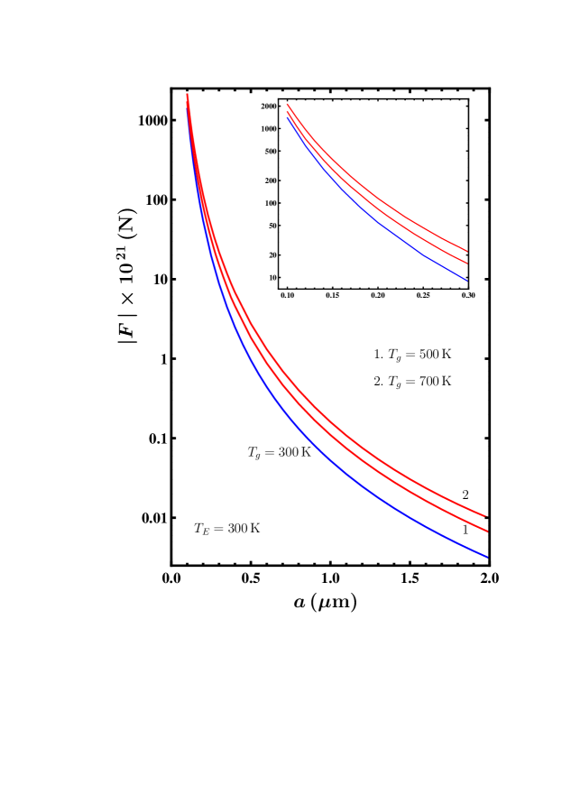
Figure 2: The magnitude of nonequilibrium Casimir-Polder force between a metallic nanoparticle of diameter 5 nm and a heated graphene sheet is shown as the function of separation by the lines 1 and 2 for two different graphene temperatures $T_{g}$. The respective equilibrium force is shown by the bottom line. The region of short separations is shown in the inset on an enlarged scale.

In Fig. 2, the computational results for the magnitude of the Casimir-Polder force, ${F_{\rm neq}}{(a,T_{E},T_{g})}$, between a metallic nanoparticle of $d=5~{}$nm diameter and a graphene sheet are presented as the functions of separation in a logarithmic scale by the lines labeled 1 and 2 for $T_{g}=500~{}$K and 700 K, respectively, in comparison with the equilibrium force, ${F_{\rm eq}}(a,T_{E})$ calculated with $T_{g}=T_{E}=300~{}$K, shown by the bottom line. In the inset, the region of short nanoparticle-graphene separations is shown on an enlarged scale. All force in Fig. 2 are negative which corresponds to attraction. It is seen that with increasing temperature the magnitude of the Casimir-Polder force increases which leads to stronger attraction.

Similar results for the case of graphene sheet cooled down to $T_{g}=77~{}$K are shown in Fig. 3. Here, the bottom line demonstrates the magnitude of the total nonequilibrium Casimir-Polder force, ${F_{\rm neq}}{(a,T_{E},T_{g})}$, which vanishes at $a\approx 0.8~{}\mu$m and becomes repulsive at larger separations. The top line reproduces the bottom line of Fig. 2 which shows the equilibrium Casimir-Polder force, ${F_{\rm eq}}(a,T_{E})$, computed with $T_{g}=T_{E}=300~{}$K. The inset again presents the region of short separations on an enlarged scale. Although the force magnitude at $T_{g}=T_{E}=300~{}$K is again larger than at $T_{g}=77~{}$K, the qualitatively new effect arising at $T_{g}<T_{E}$ is the change of attraction with repulsion for sufficiently large separations between a nanoparticle and a graphene sheet.

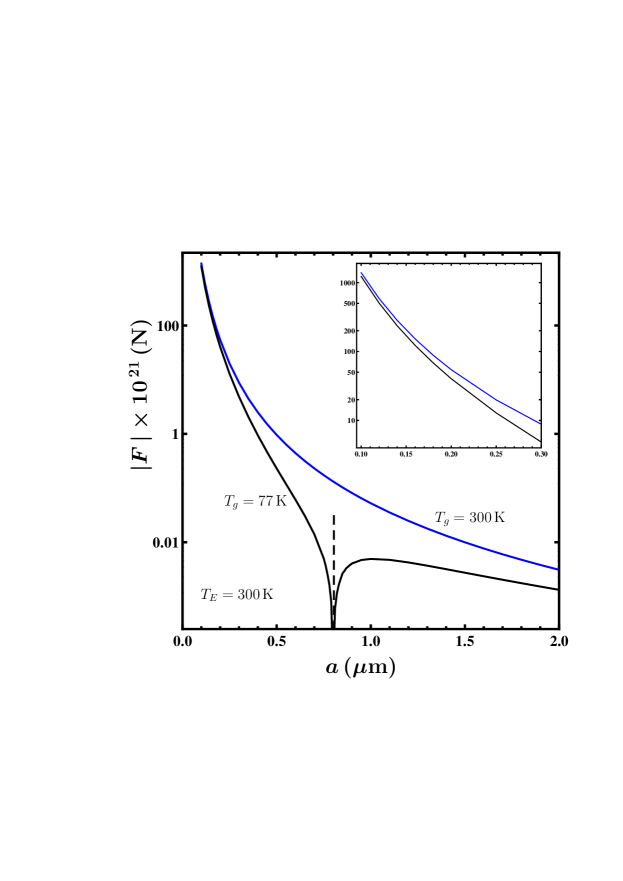
Figure 3: The magnitude of nonequilibrium Casimir-Polder force between a metallic nanoparticle of diameter 5 nm and a cooled graphene sheet is shown as the function of separation by the bottom line. The force is attractive to the left of the dashed line and repulsive to the right of it. The respective equilibrium force is shown by the top line. The region of short separations is shown in the inset on an enlarged scale.

V Conclusions and outlook

In the foregoing, we have considered the Casimir-Polder interaction between a spherical nanoparticle and a graphene sheet in out-of-thermal-equilibrium conditions when the common temperature of a nanoparticle and of the environment can be different from the temperature of graphene. This problem is of interest for both fundamental and applied physics because the electromagnetic response of graphene strongly depends on temperature. The obtained expression for the Casimir-Polder force between a nanoparticle and a graphene sheet is based on the theory of atom-wall interaction out of thermal equilibrium 6 ; 7 ; 8 ; 9 ; 10 ; 11 adapted for the case of temperature-dependent dielectric response in Ref. 12 . In so doing, the response function of graphene is described by means of the polarization tensor in the framework of the Dirac model.

In accordance to the results obtained, the magnitude of the Casimir-Polder force on a nanoparticle increases with increasing temperature of a graphene sheet although an impact of the nonequilibrium conditions decreases with increasing separation. An important qualitative effect is that at some separation distance the attractive nanoparticle-graphene force vanishes if the graphene temperature is lower than the temperature of the environment and becomes repulsive at larger separations. For a small sphere interacting with a dielectric plate characterized by the temperature-independent permittivity function, similar nonequilibrium effects were obtained in Ref. 20a at separation distances of a few micrometers. According to our results, in the case of graphene the effects of thermal nonequilibrium become essential at much shorter separation distances. This opens novel opportunities for the experimental investigation of graphene systems and for the control of forces between nanoparticles and graphene sheet with the aim of applications in bioelectronics.

References

- (1) H. B. G. Casimir and D. Polder, The influence of retardation on the London–van der Waals forces, Phys. Rev. 73, 360 (1948).
- (2) I. E. Dzyaloshinskii, E. M. Lifshitz, and L. P. Pitaevskii, General theory of van der Waals forces, Usp. Fiz. Nauk 73, 381 (1961) [Sov. Phys. Usp. 4, 153 (1961)].
- (3) E. M. Lifshitz and L. P. Pitaevskii, Statistical Physics, Part II (Pergamon, Oxford, 1980).
- (4) M. Bordag, G. L. Klimchitskaya, U. Mohideen, and V. M. Mostepanenko, Advances in the Casimir Effect (Oxford University Press, Oxford, 2015).
- (5) S. Y. Buhmann, Dispersion Forces, I, II (Springer, Berlin, 2012).
- (6) C. Henkel, K. Joulain, J.-P. Mulet, and J.-J. Greffet, Radiation forces on small particles in thermal near fields, J. Opt. A: Pure Appl. Opt. 4, S109 (2002).
- (7) M. Antezza, L. P. Pitaevskii, and S. Stringari, New Asymptotic Behavior of the Surface-Atom Force out of Thermal Equilibrium, Phys. Rev. Lett. 95, 113202 (2005).
- (8) M. Antezza, L. P. Pitaevskii, S. Stringari, and V. B. Svetovoy, Casimir-Lifshitz force out of thermal equilibrium, Phys. Rev. A 77, 022901 (2008).
- (9) G. Bimonte, Scattering approach to Casimir forces and radiative heat transfer for nanostructured surfaces out of thermal equilibrium, Phys. Rev. A 80, 042102 (2009).
- (10) R. Messina and M. Antezza, Scattering-matrix approach to Casimir-Lifshitz force and heat transfer out of thermal equilibrium between arbitrary bodies, Phys. Rev. A 84, 042102 (2011).
- (11) M. Krüger, G. Bimonte, T. Emig, and M. Kardar, Trace formulas for nonequilibrium Casimir interactions, heat radiation, and heat transfer for arbitrary bodies, Phys. Rev. B 86, 115423 (2012).
- (12) G.-L. Ingold, G. L. Klimchitskaya, and V. M. Mostepanenko, Nonequilibrium effects in the Casimir force between two similar metallic plates kept at different temperatures, Phys. Rev. A 101, 032506 (2020).
- (13) S. G. Castillo-López, R. Esquivel-Sirvent, G. Pirruccio, and C. Villarreal, Casimir forces out of thermal equilibrium near a superconducting transition, Sci. Rep. 12, 2905 (2022).
- (14) G. Bimonte, T. Emig, M. Krüger, and M. Kardar, Dilution and resonance-enhanced repulsion in nonequilibrium fluctuation forces, Phys. Rev. A 84, 042503 (2011).
- (15) W. Sun, Interaction forces between a spherical nanoparticle and a flat surface, Phys. Chem. Chem. Phys. 16, 5846 (2014).
- (16) F. Moreno, B. Garc a-Cámara, J. M. Saiz, and F. González, Interaction of nanoparticles with substrates: effects on the dipolar behaviour of the particles, Optics Express 16, 12487 (2008).
- (17) X. Luo, A. Morrin, A. J. Killard, and M. R. Smyth, Application of Nanoparticles in Electrochemical Sensors and Biosensors, Electroanalysis, 18, 319 (2006).
- (18) I. Willner, R. Baron, and B. Willner, Integrated nanoparticle-biomolecule systems for biosensing and bioelectronics, Biosens. Bioelectron. 22, 1841 (2007).
- (19) D. Dyubo and O. Yu. Tsybin, Computer Simulation of a Surface Charge Nanobiosensor with Internal Signal Integration, Biosensors 11, 397 (2021).
- (20) D. Dyubo and O. Yu. Tsybin, Particles-on-surface sensor with potential barriers embedded in a semiconductor target, J. Phys.: Conf. Ser. 1326, 012003 (2019).
- (21) M. Krüger, T. Emig, G. Bimonte, and M. Kardar, Non-equilibrium Casimir forces: Spheres and sphere-plate, Europhys. Lett. 95, 21002 (2011).
- (22) C. Khandekar, S. Buddhiraju, P. R. Wilkinson, J. K. Gimzewski, A. W. Rodriguez, C. Chase, and S. Fan, Nonequilibrium lateral force and torque by thermally excited nonreciprocal surface electromagnetic waves, Phys. Rev. B 104, 245433 (2021).
- (23) A. H. Castro Neto, F. Guinea, N. M. R. Peres, K. S. Novoselov, and A. K. Geim, The electronic properties of graphene, Rev. Mod. Phys. 81, 109 (2009).
- (24) Physics of Graphene, edited by H. Aoki and M. S. Dresselhaus (Springer, Cham, 2014).
- (25) M. I. Katsnelson, The Physics of Graphene (Cambridge University Press, Cambridge, 2020).
- (26) T. Zhu, M. Antezza, and J.-S. Wang, Dynamical polarizability of graphene with spatial dispersion, Phys. Rev. B 103, 125421 (2021).
- (27) T. E. Judd, R. G. Scott, A. M. Martin, B. Kaczmarek, and T. M. Fromhold, Quantum reflection of ultracold atoms from thin films, graphene and semiconductor heterostructures, New J. Phys. 13, 083020 (2011).
- (28) M. Chaichian, G. L. Klimchitskaya, V. M. Mostepanenko, and A. Tureanu, Thermal Casimir-Polder interaction of different atoms with graphene, Phys. Rev. A 86, 012515 (2012).
- (29) B. Arora, H. Kaur, and B. K. Sahoo, coefficients for the alkali atoms interacting with a graphene and carbon nanotube, J. Phys. B 47, 155002 (2014).
- (30) K. Kaur, J. Kaur, B. Arora, and B. K. Sahoo, Emending thermal dispersion interaction of Li, Na, K and Rb alkali-metal atoms with graphene in the Dirac model, Phys. Rev. B 90, 245405 (2014).
- (31) G. L. Klimchitskaya and V. M. Mostepanenko, Impact of graphene coating on the atom-plate interaction, Phys. Rev. A 89, 062508 (2014).
- (32) T. Cysne, W. J. M. Kort-Kamp, D. Oliver, F. A. Pinheiro, F. S. S. Rosa, and C. Farina, Tuning the Casimir-Polder interaction via magneto-optical effects in graphene, Phys. Rev. A 90, 052511 (2014).
- (33) K. Kaur, B. Arora, and B. K. Sahoo, Dispersion coefficients for the interactions of the alkali-metal and alkaline-earth-metal ions and inert-gas atoms with a graphene layer, Phys. Rev. A 92, 032704 (2015).
- (34) C. Henkel, G. L. Klimchitskaya, and V. M. Mostepanenko, Influence of chemical potential on the Casimir-Polder interaction between an atom and gapped graphene or graphene-coated substrate, Phys. Rev. A 97, 032504 (2018).
- (35) N. Khusnutdinov, R. Kashapov, and L. M. Woods, Casimir-Polder effect for a stack of conductive planes, Phys. Rev. A 94, 012513 (2016).
- (36) N. Khusnutdinov, R. Kashapov, and L. M. Woods, Thermal Casimir and Casimir-Polder interactions in N parallel 2D Dirac materials, 2D Materials 5, 035032 (2018).
- (37) G. L. Klimchitskaya and V. M. Mostepanenko, Nernst heat theorem for an atom interacting with graphene: Dirac model with nonzero energy gap and chemical potential, Phys. Rev. D 101, 116003 (2020).
- (38) N. Khusnutdinov and N. Emelianova, The Low-Temperature Expansion of the Casimir-Polder Free Energy of an Atom with Graphene, Universe 7, 70 (2021).
- (39) B. Das, B. Choudhury, A. Gomathi, A. K. Manna, S. K. Pati, and C. N. R. Rao, Interaction of Inorganic Nanoparticles with Graphene, ChemPhysChem 12, 937 (2011)
- (40) S.-A. Biehs and G. S. Agarwal, Anisotropy enhancement of the Casimir-Polder force between a nanoparticle and graphene, Phys. Rev. A 90, 042510 (2014); 91, 039901(E) (2015).
- (41) J. M. Devi, Simulation Studies on the Interaction of Graphene and Gold Nanoparticle, Int. J. Nanosci. 17, 1760043 (2018).
- (42) S. Low and Y.-S. Shon, Molecular interactions between pre-formed metal nanoparticles and graphene families, Adv. Nano Res. 6, 357 (2018).
- (43) L.-W. Huang, H.-T. Jeng, W.-B. Sua, and C.-S. Chang, Indirect interactions of metal nanoparticles through graphene, Carbon 174, 132 (2021).
- (44) G. Williams and P. V. Kamat, Graphene-Semiconductor Nanocomposites: Excited-State Interactions between ZnO Nanoparticles and Graphene Oxide, Langmuir 25, 13869 (2009).
- (45) M. Donnelly, D. Mao, J. Park, and G. Xu, Graphene field-effect transistors: the road to bioelectronics, J. Phys. D: Appl. Phys. 51, 493001 (2018).
- (46) E. Puigpelat, J. Ignés-Mullol, F. Sagués, and Ra. Reigada, Interaction of Graphene Nanoparticles and Lipid Membranes Displaying Different Liquid Orderings: A Molecular Dynamics Study, Langmuir 35, 16661 (2019).
- (47) H. Liu, C. Hao, Y. Zhang, H. Yang, and R. Sun, The interaction of graphene oxide-silver nanoparticles with trypsin: Insights from adsorption behaviors, conformational structure and enzymatic activity investigations, Coll. Surf. B: Biointerf. 202, 111688 (2021).
- (48) G. L. Klimchitskaya, V. M. Mostepanenko, and E. N. Velichko, Casimir pressure in peptide films on metallic substrates: Change of sign via graphene coating, Phys. Rev. B 103, 245421 (2021).
- (49) M. Bordag, I. V. Fialkovsky, D. M. Gitman, and D. V. Vassilevich, Casimir interaction between a perfect conductor and graphene described by the Dirac model, Phys. Rev. B 80, 245406 (2009).
- (50) I. V. Fialkovsky, V. N. Marachevsky, and D. V. Vassilevich, Finite-temperature Casimir effect for graphene, Phys. Rev. B 84, 035446 (2011).
- (51) M. Bordag, G. L. Klimchitskaya, V. M. Mostepanenko, and V. M. Petrov, Quantum field theoretical description for the reflectivity of graphene, Phys. Rev. D 91, 045037 (2015); 93, 089907(E) (2016).
- (52) M. Bordag, I. Fialkovskiy, and D. Vassilevich, Enhanced Casimir effect for doped graphene, Phys. Rev. B 93, 075414 (2016); 95, 119905(E) (2017).
- (53) G. Gómez-Santos, Thermal van der Waals interaction between graphene layers, Phys. Rev. B 80, 245424 (2009).
- (54) M. Liu, Y. Zhang, G. L. Klimchitskaya, V. M. Mostepanenko, and U. Mohideen, Demonstration of Unusual Thermal Effect in the Casimir Force from Graphene, Phys. Rev. Lett. 126, 206802 (2021).
- (55) M. Liu, Y. Zhang, G. L. Klimchitskaya, V. M. Mostepanenko, and U. Mohideen, Experimental and theoretical investigation of the thermal effect in the Casimir interaction from graphene, Phys. Rev. B 104, 085436 (2021).
- (56) G. L. Klimchitskaya, U. Mohideen, and V. M. Mostepanenko, Theory of the Casimir interaction for graphene-coated substrates using the polarization tensor and comparison with experiment, Phys. Rev. B 89, 115419 (2014).
- (57) M. Bordag and I. G. Pirozhenko, Surface plasmon on graphene at finite , Int. J. Mod. Phys. B 30, 1650120 (2016).
- (58) G. L. Klimchitskaya and V. M. Mostepanenko, Origin of large thermal effect in the Casimir interaction between two graphene sheets, Phys. Rev. B 91, 174501 (2015).
- (59) M. Bordag, G. L. Klimchitskaya, and V. M. Mostepanenko, Thermal Casimir effect in the interaction of graphene with dielectrics and metals, Phys. Rev. B 86, 165429 (2012).
- (60) G. L. Klimchitskaya and V. M. Mostepanenko, Van der Waals and Casimir interactions between two graphene sheets, Phys. Rev. B 87, 075439 (2013).