The Oscillatory Universe, phantom crossing and the Hubble tension

Abstract

We investigate the validity of cosmological models with an oscillating scale factor in relation to late-time cosmological observations. We show that these models not only meet the required late time observational constraints, but can also alleviate the Hubble tension. As a generic feature of the model, the Hubble parameter increases near the current epoch due to its cyclical nature exhibiting the phantom nature allowing to address the said issue related to late time acceleration.

1 Introduction

One of the fundamental concerns of cosmology is the late-time accelerated expansion of the universe [4, 5], which is possibly driven by the presence of a Dark energy (DE) component. Even if the $\Lambda$CDM ($\Lambda$ is the Cosmological constant and CDM is the Cold Dark Matter) is statistically most supported by observations, the fine-tuning and coincidence problem associated with it motivates one to look for alternative theories of gravity [6, 3, 7]. As we know that cosmological observations are in good agreement with the $\Lambda$CDM model with high precision, they still allow a narrow but sufficient room for the existence of weakly dynamical DE cosmological models. In this context, a variety of scalar fields inspired by high energy physics and phenomenological viewpoints have been examined in the literature to describe the late time acceleration [1, 2, 3].

Apart from being well-suited, atleast, for the high-redshift measurements, $\Lambda$CDM is confronted with the low-redshift data which measures a larger value of the Hubble constant $H_{0}$. In particular, the observational value of $H_{{}_{0}}$ found by Planck satellite is $67.36\pm 0.54$ Km/s/Mpc, whereas, low-redshift surveys, such as the Supernovae $H_{{}_{0}}$ for the Equation of State (SH0ES) collaboration finds $H_{{}_{0}}=73.04\pm 1.04$ Km/s/Mpc [8], Megamaser Cosmology Project finds $73.9\pm 3.0$ Km/s/Mpc, and H0LiCOW finds $73.3^{+1.7}_{-1.8}$ Km/s/Mpc. This large discrepancy between high and low-redshift measurements of $H_{{}_{0}}$ which is up to $4.2\sigma$ level has given a lot of attention to alternative cosmological models which even if cannot completely alleviate this ‘tension’ completely, at least try to reduce it to some extent [9, 10, 11, 12, 13, 14, 15, 16, 17, 18, 19].

Despite the existence of several scalar field DE models or modified gravity theories that might ease this tension, the problem can also be seen from a completely other viewpoint that takes into account the universe’s oscillatory characteristic. The Quasi Steady State Cosmology (QSSC), in instance, is one such domain of cosmology that permits the universe’s scale factor to oscillate rather than increase monotonically. It is an alternative cosmological theory developed in [20] and further discussed in [21], [22]. In the literature, the theoretical framework and exact solutions [23, 24], light nuclei production [25, 26, 27], structure formation [28], some observational tests [29, 30] and stability of the model [31] have already been discussed. In recent times, QSSC scenarios have also been explored with respect to the late-time observations [32, 33, 34, 35, 36, 37, 38, 39]. One of the significant feature of QSSC is that the model is free from initial singularity problem and also capable of explaining the accelerated expansion of the Universe. So, it is interesting to study QSSC to look for some more scope to resolve some fundamental problems. Here, in this paper, we are intended to work on the Hubble tension and see the possibility of resolving Hubble tension by QSSC. One of the most important features of QSSC scenarios is that they avoid any Big-Bang singularities while still explaining late-time cosmic acceleration and their potential to solve the Hubble tension problem.

Our major goal in this paper is to investigate the late-time cosmological evolution using QSSC and to determine the amount of Hubble tension relieved owing to the oscillatory character of the Hubble parameter $H(t)$. QSSC is effective of tracing back the evolutionary history of the universe at least at the background level up to large redshifts without defining any type of fluid or field. Fluid with equation of state parameter $w_{x}\gtrsim-1$ always gives rise to $\dot{H}\lesssim 0$ (where ${}^{\cdot}\equiv d/dt$, and $t$ is the cosmic time), therefore in order to have a supper acceleration $\dot{H}\gtrsim 0$ one requires $w_{x}\lesssim-1$. It was demonstrated in Ref [40], that one needs at least two fields for consistent realization of the late-time enhancement in the Hubble parameter. Indeed, one can formally construct single scalar field which gives rise to transition across the phantom divide [41]. However, such transitions are physically implausible in single field models as they are either realized by a discrete set of trajectories in the phase space or are unstable under cosmological perturbations. To describe the said behaviour consistently, one may use two field framework dubbed quintom models [42, 43, 44]. However, it is possible to realize $w_{x}\lesssim-1$ with one scalar field in scalar-tensor gravity e.g. In Ref [45, 46], the reconstruction of expansion law in modified gravity is discussed.

The layout of our paper is as follows: The section 1 provides a short introduction on dark energy and Hubble tension. In section 2, in a typical flat-Friedmann universe, we first present a brief cosmic background description of the QSSC model, then in section 3, we describe the technical details of our statistical analysis done using the Monte Carlo Markov Chain (MCMC) simulations using observational datasets. Finally, a summary and the conclusions of this work are given in section 4.

2 Background level framework of QSSC

Let us begin with a consideration that the oscillatory universe satisfies the conditions of homogeneity and isotropy and thus can be described by the standard FRW metric: $ds^{2}=dt^{2}-a(t)^{2}dr^{2}$ ($t$:= comoving time, $a(t)$:= scale factor, and $r$:= comoving distance). Unlike the common perspective of the universe in the standard FRW universe, which holds that it only expands with time, the QSSC model provides a more generalised view to this. This not only supports our universe’s traditional evolutionary paradigm (at least in the long run), but it also solves the challenges related with singularities. In fact, the crucial aspect to consider QSSC model lies in its ability to give rise to a cosmological scenario which allows our Universe to not just keep expanding but also to contract in different cycles of its evolution. Because the scale factor encodes our Universe’s time-evolutionary profile, one might suggest the following form of the scale factor to actualize such an oscillatory universe:

$$a(t)=\exp\left(\frac{t}{P}\right)\left[1+\eta\cos\frac{2\pi t}{Q}\right]\,,$$ (1)

where $P$ and $Q$ have dimensions of time, and $\eta$ is a dimensionless constant. This choice of the form of the scale factor is well described in a series of papers by Hoyle, Burbidge and Narlikar [20], [21], [22], [23], [24]. The main essence in this parametrization of $a(t)$ lies in follows:

• In the limit $\eta\rightarrow 0$ it gives rise to de-Sitter like evolution.

• In the limit $t\rightarrow 0$, $a(t)\rightarrow 1+\eta$. Thus, the standard Big-Bang singularity does not occur in QSSC scenarios.

As $P$ and $Q$ are both dimensional quantities, let us make following propositions:

$$P=\alpha t_{0}\,,\quad Q=\beta t_{0}\,,$$ (2)

where $\alpha$ and $\beta$, by definitions, are dimensionless parameters, and $t_{0}$ is the present value of the cosmic time $t$.

Consequently, the Hubble parameter $H(t)$ from Eq. (1) is expressed as

$$H(t):=\frac{\dot{a}(t)}{a(t)}=\frac{1}{\alpha t_{0}}-\frac{2\pi\eta\sin(\zeta_{t})}{\beta\left[1+\eta\cos(\zeta_{t})\right]t_{0}}\,,\qquad\mbox{where}\quad\zeta_{t}=\frac{2\pi t}{\beta t_{0}}\,.$$ (3)

Note that when $\eta\to 0$, the oscillatory behavior of the universe ceases to exist and the Hubble parameter becomes constant.

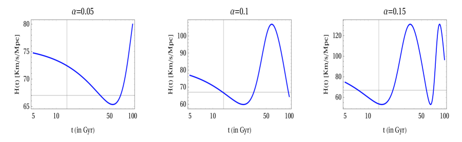
(a) For $\beta=0.7$ and $\eta=0.3$

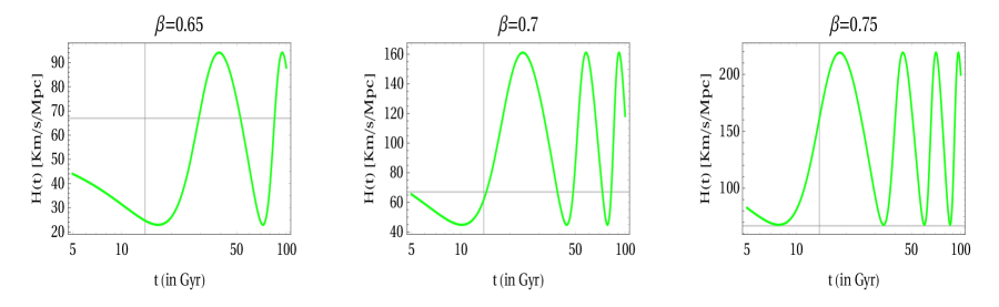
(b) For $\alpha=0.2$ and $\eta=0.3$

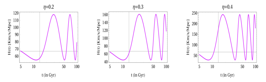
(c) For $\alpha=0.2$ and $\beta=0.7$

Figure 1: Evolution of $H(t)$ with cosmic time $t$ for different set of fiducial values of $\alpha$, $\beta$ and $\eta$. The horizontal and vertical lines represents the observed value of the Hubble constant (i.e. $67$  Km/s/Mpc) and the age of the universe, respectively.

From the above equation, one can extract out the present value of cosmic time i.e. $t_{0}$ in terms of $H_{0}$ as

$$t_{0}=\frac{1}{\alpha H_{0}}-\frac{2\pi\eta\sin(\zeta_{0})}{\beta H_{0}\left[1+\eta\cos(\zeta_{0})\right]}\,,\qquad\mbox{where}\quad\zeta_{0}=\frac{2\pi}{\beta}\,.$$ (4)

One may note that in order to realize a standard non-oscillatory Universe, $\eta$ must vanish which also make the cosmological evolution independent of $\beta$. As a result, the frequency of oscillations due to $\beta$ is controlled by parameter $\eta$. It is also interesting to note that the remaining parameter $\alpha$, then, can be treated as the power of time in the standard cosmological evolutionary profiles of $a(t)$, such as $1/2$ and $2/3$ in radiation and matter dominated era, respectively.

In order to find the $\Lambda$CDM limit(s) of QSSC model, we first identify the total equation of state parameter $w_{{}_{tot}}$ in the latter, which is defined as

$$w_{{}_{tot}}(t)=-1-\frac{2}{3}\,\frac{\dot{H}(t)}{H(t)^{2}}\,,$$ (5)

such that $\dot{H}(t)$ is given by

$$\dot{H}(t)=\frac{4H^{2}\pi^{2}\alpha^{2}\eta(1+\eta\cos(\zeta_{0}))^{2}\mathcal{X}(t)}{\mathcal{Y}(t)^{2}\left[\beta(1+\eta\cos\zeta_{0})-2\pi\alpha\eta\sin(\zeta_{0})\right]^{2}}\,,$$ (6)

where

$$\mathcal{X}(t)=\eta+\cos\left(\frac{2H\pi\,t}{\frac{\beta}{\alpha}-\frac{2\pi\eta\sin(\zeta_{0})}{1+\eta\cos(\zeta_{0})}}\right)\,,\quad\mathcal{Y}(t)=1+\eta\cos\left(\frac{2H\pi\,t}{\frac{\beta}{\alpha}-\frac{2\pi\eta\sin(\zeta_{0})}{1+\eta\cos(\zeta_{0})}}\right)\,.$$

Using Eqs. (3), (5) and (6), one can calculate the evolution of $w_{{}_{tot}}$ for a given parametric values of model parameters. In order to estimate the effective DE equation of state parameter for QSSC model, let us make use of the total equation of state expression i.e.

$$w_{{}_{tot}}=w_{{}_{DE}}\Omega_{{}_{DE}}+w_{{}_{M}}\Omega_{{}_{M}}$$ (7)

where $\Omega_{{}_{M}}$ is the matter density parameter. Since, matter is considered to be pressure-less, therefore, one can take $w_{{}_{M}}=0$. Due to the numerical complications involve in QSSC to extract out the exact profile of DE equation of state, we therefore restrict ourselves to the present epoch ($z=0$) only. By combining Eqs. (5) and (7), and taking fiducial values $H_{0}=70$ Km/s/Mpc and $\Omega_{{}_{DE}}=0.67$, we can determine our parametric ranges which can give us the $\Lambda$CDM limit i.e. $w_{{}_{DE}}(0)=-1$. In figs. (2) (a) and (b) we depict the contour lines for different values of $\alpha$ and $\beta$ which corresponds to the $\Lambda$CDM case at the present epoch.

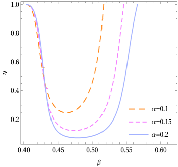
(a) For fiducial values of $\alpha$

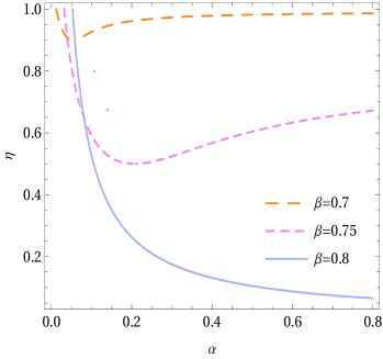
(b) For fiducial values of $\beta$

Figure 2: Contours of figs. (a) and (b) represent cases when the QSSC model reduces to the $\Lambda$CDM model with DE equation of state equal to $-1$.

In order to estimate our set of four parameters $p=\{\alpha,\beta,\eta,h\}$ ($h=H_{0}/(100\,km/s/Mpc)$), one has to express Eq. (3) in terms of redshift $z$ or scale factor $a(t)$. However, due to the complicated expression of Eq. (1), exact analytical form of $t$ in terms of $a(t)$ or $z$ is difficult to obtain. Hence, we numerically evaluate $t$ from Eq. (1) and then put it back in Eq. (3). In this way, one can evaluate $H(z)$ which can be used for parametric estimations using observational datasets. However, as we see that the scale factor $a(t)$ is not normalized at the present time $t_{0}$, hence the redshift $z$ is related to scale factor as

$$1+z=\frac{a(t_{0})}{a(t)}\,,\quad\mbox{where}\quad a(t_{0})=\exp\left(\frac{1}{\alpha}\right)\left[1+\eta\cos(\zeta_{0})\right]\,.$$ (8)

One may also note that in order to be compatible with observations which although does not signal any kind of oscillatory behaviour of the universe atleast in the past, the oscillatory behaviour of the scale factor will be tightly constrained. In fact, the parameter $\eta$ must be less than unity and its any non-zero value will cause the oscillations. Also, the time period of oscillations should be equal to or greater than the age of the universe otherwise it can affect several stringent constraints imposed by CMB observations, type Ia supernovae, LSS, etc..

With above formulation, we can now proceed to perform our data analysis in the next section.

3 Observational constraints on QSSC

For our parametric estimations, we perform the Markov Chain Monte Carlo simulation on our model using the $H(z)$+Pantheon(binned)+BAO dataset. In order to do that, we define the Likelihood function $\mathcal{L}$ as

$$\mathcal{L}\propto\exp\left(-\frac{\chi^{2}}{2}\right)\,.$$ (9)

In our parametric estimations, we take a set of thirty $H(z)$ measurements in the range $z\in[0.07,1.965]$ given in [47]. For the Supernova Type-Ia Pantheon, we take Hubble rate $E(z_{i})=H(z_{i})/H_{0}$ data points for six different redshifts within the range $z=0.07$ to $z=1.5$ presented by Reiss et al in [48]. This effectively compressing the informations of the - Pantheon compilation [49] and 15 SnIa at $z>1$ of the CANDELS and CLASH Multy-Cycle Treasury (MCT) programs obtained by the HST, nine of which are at $1.5<z<2.3$. We have also omitted the data point at $z=1.5$ which does not follow a Gaussian distribution (see [50] for more details). In addition, we take two points for BAO Lyman-$\alpha$ .

Hence, for combined dataset, the individual $\chi^{2}$ gets added to give

$$\chi_{total}^{2}=\chi_{OHD}^{2}+\chi_{Pan}^{2}+\chi_{BAO}^{2}\,.$$ (10)

Though the $SH0ES$ Collaboration measured the SN absolute magnitude directly, the difference may be less significant for late-time adjustments, such as changing the universe’s expansion pace, than it may be for early-time modifications [51, 52]. However, we make an effort to fit our model for a Gaussian prior to the Hubble constant measurement provided by the $SH0ES$ Collaboration and in order to run our MCMC simulation, we give the following prior range for our parameters:

Parameters	Priors
$\alpha$	[-0.3 , 0.3 ]
$\beta$	[0.5, 1]
$\eta$	[0, 0.5]
$h$	[0.55 ,0.85 ]

Table 1: Priors for the MCMC parameters

The obtained $2\sigma$ parametric contours between our set of parameters $\alpha$, $\beta$, $\eta$, $h$ are shown in fig. (3). In that plot one can see that the allowed parametric region for combined dataset is, as expected, smaller than that of the OHD. Also, one observes high correlation of $\eta$ with both $\alpha$ and $\beta$. The estimated values of our parameters are enlisted below. It is interesting to note that the estimated value of the Hubble constant $h$ tends to be higher than that of the $\Lambda$CDM model for both of the datasets. Let us here emphasize that this enhancement in the value of $h$ for QSSC model, is because of its oscillatory nature.

$$\alpha=0.154^{+0.032}_{-0.028}\,,\quad\beta=0.760^{+0.011}_{-0.011}\,,\quad\eta=0.366^{+0.091}_{-0.077}\,,\quad h=0.718^{+0.018}_{-0.019}\,.$$ (11)

With the above best-fit estimations, we plot the evolutionary behavior of $H(z)$ with $z$ in fig. (4). In that figure, one can see that $H(z)$ naturally tends to increase towards the current epoch which is compatible with the low-redshift Hubble observations such as Riess et al. [Riess]. This enhancement in $h$ not just come out naturally in QSSC scenarios, but it also explain the large value of the Hubble constant from the low-$z$ observations. From above estimate on $h$ we find that QSSC significantly reduces the Hubble tension between high and low redshift observations. In particular, we find that our estimate on $h$ is well within $1\sigma$ level with low-$z$ observations which removes the existing tension on the Hubble constant. Moreover, This model converges to $\Lambda$CDM in the past. Deviations from it appear only around the present epoch, where Hubble starts increasing, mimicking a late time phantom phase. Thereby, the model is as consistent with CMB as $\Lambda$CDM.

Let us note that the model under consideration has no one to one correspondence with the standard DE models, which directly take into account the amount of matter and DE densities. Since, estimating the respective densities is difficult in this case, therefore, in order to estimate the corresponding DE equation of state parameter $w_{{}_{DE}}$, we consider Planck 2018 results best-fit for DE matter density parameter $\Omega_{{}_{DE}}$.

From Eqs. (7) and (5) and using the best-fits given in (11), one can estimate $w_{{}_{DE}}$ and the present age of the universe $t(0)$ from Eq. (4) as

$$t(0)=45.05\leavevmode\nobreak\ Gyr\,,\quad w_{{}_{DE}}(0)\in[-1.036,-1.011]\,.$$ (12)

Here note that the large value of the present time is consistent with the lower limit on the age of the universe i.e. $13.8$ Gyr [53, 54, 55, 56]. This is due to the fact that in QSSC scenarios the universe instead of having a Big-Bang event keep on oscillating, which as a result gives rise to large value to the age of the universe. Moreover, the age of the universe is large enough to be consistent with the age of the globular clusters. Also note that within $1\sigma$, $w_{{}_{DE}}(0)$ shows significant deviation from the $\Lambda$CDM. This implies that $w_{{}_{DE}}(0)$ has crossed the mark of $-1$ (corresponding to the $\Lambda$CDM) in the past and is currently in the phantom region. It is interesting in a sense that this happens without incorporating any kind of assumption to the DE component, but is completely stem out of the oscillatory nature of the universe.

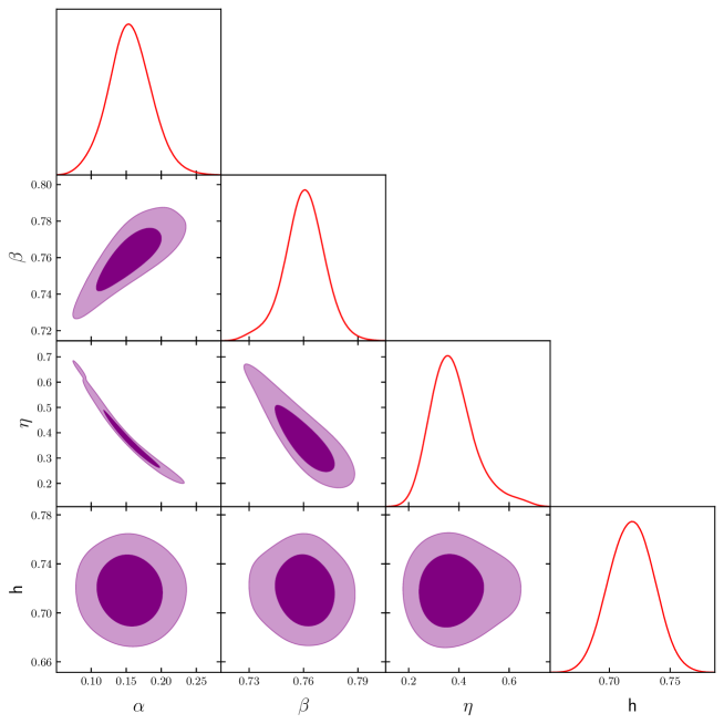
Figure 3: Upto $2\sigma$ parametric regions between $\alpha$, $\beta$, $\eta$ and $h$ for combined OHD+Pantheon+BAO dataset.

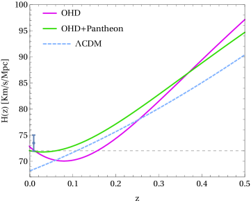
Figure 4: Evolutionary profiles of $H(z)$ with $z\in[0,0.5]$ for OHD and its combination with Pantheon dataset.

As we have shown above in fig. (4) that $H$ tends to be larger at the present epoch for the QSSC scenario, it is still intriguing or rather crucial to know whether this enhancement in $H$ or the ease of tension between the late-time and early-time cosmological data will still be preserved if one does not marginalize the absolute magnitude $M$. This is because in SH0ES actually measures the absolute magnitude $M$ of the type 1a Supernovae which are assumed to be standard candles by modulating Supernovae host galaxy distances to local geometric distance anchor via the relation of Cepheid period luminosity. Then using the magnitude-redshift relation of the Pantheon sample, the value of $H_{0}$ is calculated from the measurement of $M$. As a result, it has been hypothesized that the $H_{0}$ tension is really a tension on the supernova absolute magnitude $M$, since the SH0ES $H_{0}$ measurement is based on $M$ estimations.

Keeping in mind that the Hubble constant and absolute magnitude $M$ are highly correlated with one another, we now make a complete parametric estimation using the Pantheon and Hubble datasets on both $H_{0}$ and $M$. Our estimated parameters are enlisted below:

$$\alpha=0.163^{+0.022}_{-0.020}\,,\quad\beta=0.749^{+0.024}_{-0.017}\,,\quad\eta=0.358^{+0.062}_{-0.047}\,,\quad h=0.719^{+0.047}_{-0.049}\,,\quad M=-19.302^{+0.047}_{-0.061}$$ (13)

(a) Probability distribution of $h$.

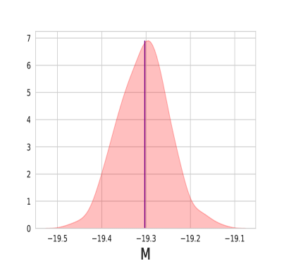
(b) Probability distribution of $M$.

Figure 5: Probability distribution functions for Hubble constant $h$ and absolute magnitude $M$. The vertical line corresponds to their corresponding best-fit values.

In above estimations, one can see that even with the supernovae absolute magnitude the value for the Hubble constant comes out to be almost the same as we have in our previous estimations (11). It shows that the QSSC model indeed predicts the enhancement of the Hubble parameter near the present epoch due to the oscillatory nature of its scale factor. Also, note that our estimation on $M$ i.e. $-19.302^{+0.047}_{-0.061}$ does not reflect any tension with its observed measurement.

4 Conclusion

In this paper, we have investigated the observational aspects of the QSSC with the possibility of resolving the Hubble tension. In principle, QSSC model involves an oscillatory behavior of the scale factor and hence the Hubble parameter. The Hubble parameter, by nature of oscillatory, gets turn around by reaching its minima near the present epoch (fig (4)). As a result, the model naturally exhibits super-acceleration expansion of the Universe due to the enhancement in the Hubble parameter which become compatible with low-redshift galaxy surveys.

One of the major requirements for the QSSC is to also be compatible with the age of the Universe. Due to its oscillatory representation of the universe, the cycle per oscillation must be greater than or equal to the age of the Universe, otherwise it may contradict the age of the some of the local galaxy clusters. In fact in our parametric estimations, we have explicitly shown that the age of the Universe is not just satisfies the lower bound $13.8$ Gyr but is even greater than $30$ Gyr which is because of the repeatedly expansions and contractions of the Universe. Notably, this is also consistent with the age of the globular clusters and the Planck constraints. We have also found that if there could be an effective DE equation of state $w_{DE}$ associated with QSSC model, which if we can also extract out from the total equation of state, which is further depend on the Hubble parameter, then that effective DE behaves as a phantom at the, atleast, present epoch. This is, however, interesting in a sense that there the phantom nature of effective DE appears naturally without the incorporation of any adhoc degree of freedom.

References

- [1] M. Sami: Lect. Notes Phys. 720, 219-256 (2007), Contribution to:3rd Aegean Summer School: TheInvisible Universe: Dark Matter and Dark Energy.
- [2] M. Sami, and R. Myrzakulov, General Relativity and Gravitation, 54(8), 1-15 (2022).
- [3] E. J. Copeland, M. Sami and S. Tsujikawa, IJMPD, 15 1753 (2006).
- [4] A. G. Riess et al., Astron. J, 116(3) 1009 (1998).
- [5] S. Perlmutter et al., Astrophys. J, 517(2) 565 (1999).
- [6] L. Amendola and S. Tsujikawa, Dark energy. Theory and observations, (Cambridge Univ. Press, Cambridge, 2010).
- [7] N. Aghanim et al., A&A, 641 A6 (2020).
- [8] Adam G. Riess et al., Astrophys. J Lett., 934 1, L7 (2022).
- [9] L. Berezhiani, J. Khoury and J. Wang,PRD, 95 (12), 123530 (2017).
- [10] V. Poulin et al., PRL, 122, 221301 (2019).
- [11] E. Di Valentino ,V. E. Linder and A. Melchiorri, PRD, 97, 043528 (2018).
- [12] S. A. Adil et al., PRD, 104 (10), 103534 (2021).
- [13] J. Sola et al., Astrophys. J Lett., 886 1, L6 (2019).
- [14] Miguel Zumalacarregui,PRD, 102 (2), 023523 (2020).
- [15] Mario Ballardini et al., JCAP, 10, 044 (2020).
- [16] Matteo Braglia et al., PRD, 103 (4), 043528 (2021).
- [17] Caterina UmiltA et al.,JCAP, 08 017 (2015).
- [18] Mario Ballardini et al., JCAP, 05 067 (2016).
- [19] Mario Ballardini et al., JCAP, 10 044 (2020).
- [20] F. Hoyle, G. Burbidge, J. V. Narlikar, Astrophys. J, 410 437 (1993).
- [21] F. Hoyle, G. Burbidge, J. V. Narlikar, MNRAS, 267(4) 1007 (1994).
- [22] F. Hoyle, G. Burbidge, J. V. Narlikar, A&A., 289(3) 729 (1994).
- [23] F. Hoyle, G. Burbidge, J. V. Narlikar, Proc. R. Soc. A, 448 191 (1995).
- [24] R. Sachs, J. V. Narlikar, F. Hoyle, A&A, 313 703 (1996).
- [25] F. Hoyle, G. Burbidge, J. V. Narlikar, Proc. ESO/EIPCR Workshop, Elba, Springer, 21 (1995).
- [26] G. Burbidge, F. Hoyle, Astrophys. J, 509 L1 (1998).
- [27] J. V. Narlikar et al., Int. J. Mod. Phys. D., 6 125 (1997).
- [28] A. Nayeri et al.,Astrophys. J, 525 10 (1999).
- [29] S. K. Banerjee, J. V. Narlikar, MNRAS, 307 73 (1999).
- [30] S. K. Banerjee et al., Astronom. J, 119(6) 2583 (2000).
- [31] S. K. Banerjee, J. V. Narlikar, Astrophys. J, 487 69 (1997).
- [32] J. V. Narlikar, Pramana, 53(6) 1093 (1999).
- [33] J. V. Narlikar, R. G. Vishwakarma, G. Burbidge, F. Hoyle, arXiv:astro-ph/0101551 [astro-ph] (2001).
- [34] J. V. Narlikar, R. G. Vishwakarma, G. Burbidge, The Astronomical Society of the Pacific, 114 1092 (2002).
- [35] J. V. Narlikar et al., Astrophy. J, 585 1 (2003).
- [36] J. V. Narlikar, Chaos, Solitons and Fractals, 16 469 (2003).
- [37] J. V. Narlikar, G. Burbidge, R. G. Vishwakarma, J. Astophys. Astron., 28 67 (2007).
- [38] R. G. Vishwakarma, J. V. Narlikar, Res. Astron. Astrophys., 10(12) 000 (2010).
- [39] J. V. Narlikar et al., MNRAS., 451 1390 (2015).
- [40] A. Vikman, PRD., 71 023515 (2005).
- [41] S. V. Chervon et al., PRD., 100 063522 (2019).
- [42] M. R. Setare, E. N. Saridakis, PRD., 79 043005 (2009).
- [43] S. Mishra, S. Chakraborty, EPJC., 78 917 (2018).
- [44] G. Leon, A. Paliathanasis, J. L. Morales-Martínez, EPJC., 78 753 (2018).
- [45] B. Boisseau et al., PRL, 85 2236 (2000).
- [46] V. Sahni, A. Starobinsky, IJMPD, 15 2105 (2006).
- [47] M. Moresco et al., JCAP, 05, 014 (2016).
- [48] A. G. Riess et al., Astrophys. J. 853 126 (2018).
- [49] D. M. Scolnic et al., Astrophys. J, 859 (2), 101 (2018).
- [50] A. Gomez-Valent and L. Amendola, J. Cosmol. Astropart. Phys. 04 (2018) 051.
- [51] G. Efstathiou, MNRAS, 505 (3), 3866 (2021).
- [52] D. Camarena, V. Marra, MNRAS, 504, 5164 (2021).
- [53] D. N. Spergel et al., Proceedings of the National Academy of Sciences, 94 6579 (1997).
- [54] J. Dunlop et al., Nature, 381 581 (1996).
- [55] I. Damjanov, et al., Astrophy. J, 695 101 (2009).
- [56] M. Salaris, S. Degl’Innocenti, And A. Weiss, Astrophy. J, 479 665 (1997).