Pick up the PACE: Fast and Simple Domain Adaptation via Ensemble Pseudo-Labeling

Abstract

Domain Adaptation (DA) has received widespread attention from deep learning researchers in recent years because of its potential to improve test accuracy with out-of-distribution labeled data. Most state-of-the-art DA algorithms require an extensive amount of hyperparameter tuning and are computationally intensive due to the large batch sizes required. In this work, we propose a fast and simple DA method consisting of three stages: (1) domain alignment by covariance matching, (2) pseudo-labeling, and (3) ensembling. We call this method PACE, for Pseudo-labels, Alignment of Covariances, and Ensembles. PACE is trained on top of fixed features extracted from an ensemble of modern pretrained backbones. PACE exceeds previous state-of-the-art by 5 - 10 % on most benchmark adaptation tasks without training a neural network. PACE reduces training time and hyperparameter tuning time by 82% and 97%, respectively, when compared to state-of-the-art DA methods. Code is released here: https://github.com/Chris210634/PACE-Domain-Adaptation

1 Introduction

Deep learning is infamous for requiring a large amount of labeled data to achieve state-of-the-art results, but in many applications, labeled data is expensive to obtain zhao2020review ; zhang2020covid ; wang2020covid . In the last few years, new sub-disciplines of deep learning have emerged to address this over-reliance on labeled data. Self-supervised learning learns useful representations of data through handcrafted augmentations instead of labels jing2020self ; jaiswal2020survey . Semi-supervised learning learns from a small amount of labeled data and a large amount of unlabeled data from the same distribution van2020survey . Domain Adaptation (DA) is similar to semi-supervised learning, but considers the case where the labeled and unlabeled data come from different distributions zhuang2020comprehensive ; wilson2020survey . We call the labeled data the source domain and the unlabeled data the target domain. For example, consider the following scenario. A company wants to train a speech recognition system for deployment in a noisy car environment (target domain). A large amount of labeled recordings is available for indoor environments (source domain), but a limited amount of labeled target data is available. DA addresses this problem by minimizing the empirical risk on source data while encouraging features to be domain invariant. We consider both Semi-supervised Domain Adaptation (SSDA) saito2019semi , where a small amount of labeled target data is available, and Unsupervised Domain Adaptation (UDA) ganin2016domain , where no labeled target data is available.

Many modern DA methods train a feature extractor and linear classifier to minimize a weighted sum of three losses: (1) cross entropy loss on labeled source data ganin2016domain ; saito2019semi ; acuna2021f ; liu2021cycle , (2) divergence loss between source and target domain features ganin2016domain ; saito2019semi ; acuna2021f ; zhang2019bridging and (3) consistency loss between augmented views of unlabeled target data singh2021clda ; li2021cross ; zhang2022low . Generally, better performing methods require large batch sizes and a large number of hyperparameters kim2020attract ; li2021cross ; liu2021cycle ; zhang2022low ; singh2021clda . For example, CDAC li2021cross , a state-of-the-art method in SSDA, requires a batch of labeled data, a batch of unlabeled data, and two augmented batches of unlabeled data. On a small feature extractor, such as ResNet34, tuning and running this method is feasible. However, scaling this type of method to large modern feature extractors would require several GPUs working in parallel liu2021swin ; liu2022convnet . Computationally efficient training is important for two reasons: (1) there is significant interest in energy-efficient training on resource-constrained edge devices wang2019e2 ; he2020group , and (2) algorithms which achieve state-of-the-art with low computational cost foster democratic research berthelot2021adamatch . This raises the question: is it possible to leverage high quality features from large modern backbones, using only one GPU, and still achieve competitive DA results? The answer is yes!

Present work: In this paper, we propose an efficient DA method PACE (Pseudo-labels, Alignment of Covariances, and Ensembles), which uses pre-deep learning DA methods on top of fixed features extracted from an ensemble of ConvNeXt liu2022convnet and Swin liu2021swin backbones pre-trained on ImageNet deng2009imagenet . Our method consists of three stages (see Figure 1): (1) We align the source and target feature distributions by matching their covariances with CORAL coral . (2) We use self-training with confidence thresholding to align the class-conditional feature distributions between source and target domains. (3) We run the first two steps with different pre-trained backbones and average the predictions. We hypothesize that the features extracted by the collection of pre-trained backbones are not perfectly correlated because of differences in pre-training and architecture. Therefore, we should observe a boost in accuracy when combining predictions from the ensemble.

Our contributions are:

• We re-visit CORAL coral , a simple method for domain alignment that is not widely used by state-of-the-art DA methods. We show that when combined with self-training and ensembling, CORAL offers a boost in target accuracy without adding much complexity.

• We propose PACE, which reduces training time and hyperparameter tuning time by 82% and 97%, respectively (see Figure 2) while exceeding state-of-the-art SSDA and UDA methods by 5-10% on most benchmark tasks (see Tables 2, 3 and 4).

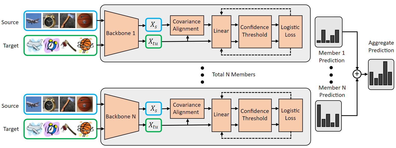
Figure 1: Illustration of the PACE framework. A solid arrow indicates a forward pass. A dashed arrow indicates a backward pass. PACE consists of three steps: (1) the source features $\mathbf{X}_{s}$ are transformed such that their covariances match the target feature $\mathbf{X}_{tu}$ covariances, (2) a linear classifier is trained with logistic loss on source data and pseudo-labeled target data, and (3) the predictions from ensemble members are averaged to return an aggregate prediction.

2 Related Work

Domain Feature Alignment

Following Ben-David et al.’s DA theory ben2010theory , DANN ganin2016domain , MCD saito2018maximum , MME saito2019semi , MDD zhang2019bridging , and f-DAL acuna2021f minimize the empirical source risk and some divergence measure between source and target distributions as a surrogate to minimizing target risk. CAN kang2019contrastive and CLDA singh2021clda use a contrastive approach to align the class-conditional feature distributions. At a high level, these methods train the backbone to output domain-invariant features and improve target accuracy over source-only training. However, the effectiveness of these methods is unclear in the context of large modern backbones, which produce good features without any fine-tuning or adaptation (Table 5). A preliminary study kim2022broad shows that some state-of-the-art DA methods attain lower target accuracy than source-only training on some benchmark adaptation tasks, due to negative transfer wang2019characterizing . It is currently unclear what target accuracy is achievable on benchmarks without any training of the backbone. We fill this gap by presenting results on benchmarks using a fast and simple DA method that does not train the backbone. We hope that these results serve as a helpful baseline for future work.

Pseudo-labeling applied to DA

Pseudo-labeling lee2013pseudo (also called self-training) is a well-established semi-supervised technique that adds artificial supervision to unlabeled data. FixMatch sohn2020fixmatch is a popular variant of self-training, which generates high-quality pseudo-labels by confidence thresholding and enforcing consistency between augmented copies of data. Many DA methods use FixMatch as part of their framework liu2021cycle ; li2021cross ; zhang2022low ; berthelot2021adamatch , so high quality pseudo-labels is important in the context of DA. Despite the success of these methods, pseudo-labeling is known to suffer from confirmation bias arazo2020pseudo . Recent studies try to mitigate this issue with meta-learning pham2021meta and debiasing chen2022debiased . Our method generates high quality pseudo-labels and can complement pseudo-labeling-based DA methods as the first stage in a DA pipeline.

Ensembling in DA

Many application-oriented deep learning studies use an ensemble of multiple deep models to boost accuracy alshazly2019ensembles ; alsafari2020deep ; rajaraman2020iteratively . Some multi-source DA methods zhou2021domain ; kang2020contrastive use an ensemble of experts trained on each source domain to obtain more accurate pseudo-labels for target data. Inspired by these studies, we incorporate an ensemble of different backbones as part of our framework and show that it increases target accuracy. We further experiment with forming an ensemble of different augmented views of the dataset. This is inspired by SENTRY prabhu2021sentry , which uses a committee of augmented views to guide training.

3 Method

Setup and Notation

We have a labeled source dataset of size $n_{s}$, a labeled target dataset of size $n_{tl}$ and an unlabeled target dataset of size $n_{tu}$. The output of the backbone is dimension $d$. We then denote the feature vectors extracted from the backbone as: $\mathbf{X}_{s}\in\mathbb{R}^{n_{s}\times d},\mathbf{X}_{tl}\in\mathbb{R}^{n_{tl}\times d},\mathbf{X}_{tu}\in\mathbb{R}^{n_{tu}\times d}$. The label vectors are denoted as $\mathbf{y}_{s}\in\mathbb{R}^{n_{s}}$ and $\mathbf{y}_{tl}\in\mathbb{R}^{n_{tl}}$ for source and labeled target, respectively. We always optimize over the entire dataset (as opposed to stochastic optimization), so for conciseness, we use the expectation symbol $\mathop{\mathbb{E}}[\cdot]$ to denote the deterministic average. When training linear classifiers, we use logistic regression, which we denote concisely as:

$$\ell(\cdot,y):=\mathop{\text{CrossEntropy}}(\mathop{\text{Softmax}}(\cdot),y)$$

Overview

We form an ensemble from all pretrained ConvNeXt-XL and Swin-L backbones available through the timm rw2019timm python library (Table 1) and perform the following steps for each ensemble member: (1) Calculate the features for all data; (2) Use CORAL to align the target and source feature distributions; (3) Train a linear classifier on all labeled data; and (4) Fine-tune the linear classifier using self-training to adjust for label shift. Finally, we output the average of ensemble predictions. See Figure 1.

3.1 CORAL feature alignment

CORAL coral is a popular linear algebraic method for distribution alignment. Its goal is to align labeled and unlabeled feature distributions by transforming the labeled data such that its covariance matrix is the same as the unlabeled data. CORAL consists of two steps. First, we whiten the labeled data distribution by subtracting the mean and normalizing covariances. Note that for this step, we concatenate the source data and labeled target data together:

$$\begin{split}\mathbf{X}_{\text{labeled}}&=\text{concatenate}(\mathbf{X}_{s},\mathbf{X}_{tl})\\ \mathbf{X}_{\text{labeled}}&=\mathbf{X}_{\text{labeled}}-\mathop{\mathbb{E}}[\mathbf{X}_{\text{labeled}}]\>,\>\mathbf{X}_{tu}=\mathbf{X}_{tu}-\mathop{\mathbb{E}}[\mathbf{X}_{tu}]\\ \mathbf{X}_{\text{labeled}}&=\mathbf{X}_{\text{labeled}}\cdot\mathbf{C}_{\text{labeled}}^{-1/2}\>\text{ where }\mathbf{C}_{\text{labeled}}=\text{Cov}(\mathbf{X}_{\text{labeled}})+\lambda I\end{split}$$ (1)

where $\lambda$ is a small numerical constant to ensure the covariance matrix is invertible. $\mathbf{X}_{\text{labeled}}$ now looks like samples from a standard normal distribution with zero-mean and unit variance. Next, we re-color the source data with the target covariance matrix:

$$\mathbf{X}_{\text{labeled}}=\mathbf{X}_{\text{labeled}}\cdot\mathbf{C}_{tu}^{1/2}\>\text{ where }\mathbf{C}_{tu}=\text{Cov}(\mathbf{X}_{tu})+\lambda I$$ (2)

The labeled and unlabeled distributions are now aligned in the sense that it is impossible to train a binary linear classifier which distinguishes the two distributions. We would hope that training a linear classifier on the recolored labeled data would yield similar accuracy between labeled and unlabeled data. However, this is not the case because of label shift. Namely, the source and target distributions, when conditioned on the labels, are not the same. In the next subsection, we use self-training to train a linear classifier which accounts for label shift.

3.2 Self Training

Following prior DA literature saito2019semi ; singh2021clda ; li2021cross , we L2-normalize the features, then train a zero-bias linear classifier on the labeled data with logistic loss. The resulting classifier is biased towards the source distribution. To adjust for this bias, we pseudo-label the target features using the source classifier and calculate confidences. We then fine-tune the classifier with the confident source and target samples, using simple confidence thresholding. The resulting classifier achieves higher target accuracy at the expense of lower source accuracy. Importantly, note that we discard source samples with low confidence, because they are unlikely to be informative of target data. Concretely, let $\mathbf{W}$ be the weight matrix of the linear classifier being trained; $\mathbf{W}\in\mathbb{R}^{K\times d}$, where $K$ is the number of classes. We repeat the following for $T$ iterations ($t\in 1:T$):

$$\begin{split}\text{Pseudo-labeling:}\>\>\>\>&\hat{\mathbf{y}}_{tu}=\mathop{\text{argmax}}\mathbf{X}_{tu}\mathbf{W}^{\top}\\ \text{Confidence Thresholding:}\>\>\>\>&\text{mask}_{s}=\mathbbm{1}[\mathbf{X}_{s}\mathbf{W}^{\top}>\tau_{t}^{s}]\>,\>\text{mask}_{tu}=\mathbbm{1}[\mathbf{X}_{tu}\mathbf{W}^{\top}>\tau_{t}^{tu}]\\ \text{Train classifier:}\>\>\>\>&\mathbf{W}=\mathop{\text{argmin}}_{\mathbf{W}}\alpha_{t}\mathcal{L}_{s}+\beta_{t}\mathcal{L}_{tl}+\gamma_{t}\mathcal{L}_{tu}\\ \mathcal{L}_{s}&:=\mathop{\mathbb{E}}[\ell(\mathbf{X}_{s}\mathbf{W}^{\top},\mathbf{y}_{s})\cdot\text{mask}_{s}]\\ \mathcal{L}_{tl}&:=\mathop{\mathbb{E}}[\ell(\mathbf{X}_{tl}\mathbf{W}^{\top},\mathbf{y}_{tl})]\\ \mathcal{L}_{tu}&:=\mathop{\mathbb{E}}[\ell(\mathbf{X}_{tu}\mathbf{W}^{\top},\hat{\mathbf{y}}_{tu})\cdot\text{mask}_{tu}]\end{split}$$ (3)

where $\tau_{t}^{s}$ and $\tau_{t}^{tu}$ are confidence thresholds for source and unlabeled target data at iteration $t$. $\alpha_{t}$, $\beta_{t}$, and $\gamma_{t}$ are hyperparameters. We solve the $\mathop{\text{argmin}}$ over $\mathbf{W}$ in Equation 3 using Gradient Descent (GD). The pseudo-labeling and classifier fine-tuning steps are repeated for a fixed number of iterations $T$. This iterative approach gradually adapts the linear classifier to the target distribution.

3.3 Ensembling

It is well known that aggregating the predictions of weak classifiers results in a strong classifier, under the assumption that the predictions of the weak classifiers are not completely correlated (Chapter 14 of bishop2006pattern ). We hypothesize that the classifiers trained on each backbone do not make completely correlated predictions. Hence, averaging the predictions from an ensemble of backbones should outperform the best member backbone. We demonstrate experimentally in Table 6 that the average prediction of the ensemble is almost always better than the best ensemble member.

Algorithm 1 PACE

Input: Labeled target data $\mathbf{X}_{tl}$, Unlabeled target data $\mathbf{X}_{tu}$, Labeled source data $\mathbf{X}_{s}$
Output: Predictions for unlabeled target data $\hat{\mathbf{y}}_{tu}$

Step 1: CORAL feature alignment. (Do for each ensemble member)
Modify $\mathbf{X}_{s}$ , $\mathbf{X}_{tl}$ and $\mathbf{X}_{tu}$ according to Equations 1 and 2.

Step 2: Train labeled classifier. (Do for each ensemble member)
L2-Normalize $\mathbf{X}_{s}$, $\mathbf{X}_{tl}$, and $\mathbf{X}_{tu}$.
Initialize weight matrix $\mathbf{W}$, then using GD with learning rate $\eta_{0}$, solve:

$$\mathbf{W}=\mathop{\text{argmin}}_{\mathbf{W}}\alpha_{0}\mathcal{L}_{s}+\beta_{0}\mathcal{L}_{tl},\>\text{where }\mathcal{L}_{s}:=\mathop{\mathbb{E}}[\ell(\mathbf{X}_{s}\mathbf{W}^{\top},\mathbf{y}_{s})],\>\mathcal{L}_{tl}:=\mathop{\mathbb{E}}[\ell(\mathbf{X}_{tl}\mathbf{W}^{\top},\mathbf{y}_{tl})]$$

Step 3: Self Training. (Do for each ensemble member)
For $t$ in $T$ iterations:
inde Use GD with learning rate $\eta_{t}$ to train $\mathbf{W}$ following Equation 3.

Step 4: Ensemble by averaging.
With some abuse of notation, we denote $\mathbf{W}_{i}$ as the weights of the $i$-th ensemble member.

$$\hat{\mathbf{y}}_{tu}=\mathop{\text{argmax}}\sum_{i}\mathop{\text{Softmax}}(\mathbf{X}_{tu}\mathbf{W}_{i}^{\top})$$

Table 1: Details on ensemble members

Model	Input	Output	Pre-train	Fine-tune	Throughput (img/sec)
	Size	Size			P100	V100
ConvNeXt-XLliu2022convnet	$384^{2}$	2048	ImageNet 22K	ImageNet 1K	13.9	27.3
ConvNeXt-XLliu2022convnet	$224^{2}$	2048	ImageNet 22K	ImageNet 1K	38.2	67.6
ConvNeXt-XLliu2022convnet	$224^{2}$	2048	ImageNet 22K	None	38.2	67.8
Swin-Lliu2021swin	$224^{2}$	1536	ImageNet 22K	ImageNet 1K	66.4	103.6
Swin-Lliu2021swin	$224^{2}$	1536	ImageNet 22K	None	64.6	91.7
Swin-Lliu2021swin	$384^{2}$	1536	ImageNet 22K	ImageNet 1K	22.1	37.1
Swin-Lliu2021swin	$384^{2}$	1536	ImageNet 22K	None	22.0	37.6

4 Experiments

Datasets

We validate our method on two common domain adaptation benchmarks: Office-Home venkateswara2017deep and DomainNet peng2019moment . Office-Home contains 15,588 images belonging to 64 classes from 4 domains: Art, Product, Real, and Clipart. Following SSDA literature, we use a subset of DomainNet saito2019semi , which contains 145,145 images belonging to 126 classes from 4 domains: Art, Painting, Real, and Clipart. For Office-Home, we present UDA results in Table 2 and 3-shot SSDA results in Table 3 on all 12 source-target combinations. For DomainNet, we present 1-shot and 3-shot SSDA results in Table 4 on 7 source-target combinations used in prior SSDA work. 1-shot means that only 1 labeled target sample per class is used; 3-shot means that 3 labeled target samples per class are used.

Baselines

We compare our UDA performance on Office-Home with baselines in Table 2. All baselines are cited inline. All baselines use ResNet-50 backbone with ImageNet-1K pretraining unless otherwise noted. We also include comparisons to recent transformer-based methods, which achieve higher target accuracy than traditional ResNet-based approaches. Some papers report results on transformer networks of varying size; we report the best result reported by the authors. We compare our SSDA performance with baselines in Tables 3 and 4. All SSDA baselines use ResNet-34 pretrained on ImageNet-1K.

Hyperparameters

We use the same set of hyperparameters across all datasets and tasks. Each ensemble member is trained with the same hyperparameters using Algorithm 1. We use GD on the entire dataset with momentum=0.9 with Nestorov correction. We do not regularize classifier weights. We tune the learning rates $\eta_{0}...\eta_{T}$ and number of GD iterations such that the loss converges to a reasonable value. $\eta_{0}=40$, $\eta_{1:T}=80$. Initial training on labeled data (Step 2) runs for 400 GD iterations, all self training steps (Step 3) run for 200 GD iterations. The remaining hyperparameters are tuned coarsely on the target validation accuracy of the SSDA 3-shot DomainNet Real to Clipart task. The initial guess for hyperparameter values is guided by the intuition that as training progresses, the classifier should rely less on source labels and more on target pseudo-labels. The final values used for all results are: $T=30$, $\alpha_{0}=0.4$, $\beta_{0}=0.2$, $\alpha_{1:T}=0.1$, $\beta_{1:T}=0.05$, $\gamma_{1:T}=0.9$, $\tau^{s}_{1:T}=0.8$, $\tau^{tu}_{1:10}=0.9$, $\tau^{tu}_{11:20}=0.8$, $\tau^{tu}_{21:30}=0.7$. See Appendix for results using different hyperparameters.

We include code and results for each ensemble member in the supplementary material.

Performance Metrics

All results are top-1 target accuracy. Following prior work, UDA target accuracy is reported over the entire target dataset (there is no training/validation/test split). In the SSDA setting, target data is split into labeled, validation and unlabeled sets. Target accuracy is reported over the unlabeled set. The validation set contains 3 target samples per class and is only used for tuning hyperparameters.

Table 2: UDA results on Office-Home. All baselines use ResNet-50he2016deep as backbone unless otherwise noted. WinTR uses DeiT-Stouvron2021training . CDTrans uses DeiT-Btouvron2021training . TVT and SSRT use ViT-Bdosovitskiy2020image . BCAT uses Swin-Bliu2021swin . Ours (small) refers to the ensemble of 7 backbones on unaugmented data. Ours (large) refers to the ensemble of 28 (7 backbones $\times$ 4 augmented views). The domains are abbreviated as A:Art, C:Clipart, P:Product, R:Real.

Method	A - C	A - P	A - R	C - A	C - P	C - R	P - A	P - C	P - R	R - A	R - C	R - P	Mean
Source-Only	34.9	50.0	58.0	37.4	41.9	46.2	38.5	31.2	60.4	53.9	41.2	59.9	46.1
DANN (JMLR ’16) ganin2016domain	45.6	59.3	70.1	47.0	58.5	60.9	46.1	43.7	68.5	63.2	51.8	76.8	57.6
JAN (ICML ’17) long2017deep	45.9	61.2	68.9	50.4	59.7	61.0	45.8	43.4	70.3	63.9	52.4	76.8	58.3
CDAN (Neurips ’18) long2018conditional	50.7	70.6	76.0	57.6	70.0	70.0	57.4	50.9	77.3	70.9	56.7	81.6	65.8
ALDA (AAAI ’20) chen2020adversarial	53.7	70.1	76.4	60.2	72.6	71.5	56.8	51.9	77.1	70.2	56.3	82.1	66.6
SAFN (ICCV ’19) xu2019larger	52.0	71.7	76.3	64.2	69.9	71.9	63.7	51.4	77.1	70.9	57.1	81.5	67.3
SymNet (CVPR ’19) zhang2019domain	47.7	72.9	78.5	64.2	71.3	74.2	64.2	48.8	79.5	74.5	52.6	82.7	67.6
TADA (AAAI ’19) wang2019transferable	53.1	72.3	77.2	59.1	71.2	72.1	59.7	53.1	78.4	72.4	60.0	82.9	67.6
MDD (ICML ’19) zhang2019bridging	54.9	73.7	77.8	60.0	71.4	71.8	61.2	53.6	78.1	72.5	60.2	82.3	68.1
BNM (CVPR ’20) cui2020towards	56.2	73.7	79.0	63.1	73.6	74.0	62.4	54.8	80.7	72.4	58.9	83.5	69.4
MDD+IA (ICML ’20) jiang2020implicit	56.2	77.9	79.2	64.4	73.1	74.4	64.2	54.2	79.9	71.2	58.1	83.1	69.5
f-DAL (ICML ’21) acuna2021f	56.7	77.0	81.1	63.1	72.2	75.9	64.5	54.4	81.0	72.3	58.4	83.7	70.0
CADA-P (CVPR ’19) kurmi2019attending	56.9	76.4	80.7	61.3	75.2	75.2	63.2	54.5	80.7	73.9	61.5	84.1	70.2
GSDA (CVPR ’20) hu2020unsupervised	61.3	76.1	79.4	65.4	73.3	74.3	65.0	53.2	80.0	72.2	60.6	83.1	70.3
GVB (CVPR ’20) cui2020gradually	57.0	74.7	79.8	64.6	74.1	74.6	65.2	55.1	81.0	74.6	59.7	84.3	70.4
DCAN (AAAI ’20) li2020domain	54.5	75.7	81.2	67.4	74.0	76.3	67.4	52.7	80.6	74.1	59.1	83.5	70.5
TCM (ICCV ’21) yue2021transporting	58.6	74.4	79.6	64.5	74.0	75.1	64.6	56.2	80.9	74.6	60.7	84.7	70.7
HDAN (Neurips ’20) cui2020heuristic	56.8	75.2	79.8	65.1	73.9	75.2	66.3	56.7	81.8	75.4	59.7	84.7	70.9
MetaAlign (CVPR ’21) wei2021metaalign	59.3	76.0	80.2	65.7	74.7	75.1	65.7	56.5	81.6	74.1	61.1	85.2	71.3
ToAlign (Neurips ’21) wei2021toalign	57.9	76.9	80.8	66.7	75.6	77.0	67.8	57.0	82.5	75.1	60.0	84.9	72.0
SENTRY (ICCV ’21) prabhu2021sentry	61.8	77.4	80.1	66.3	71.6	74.7	66.8	63.0	80.9	74.0	66.3	84.1	72.2
FixBi (CVPR ’21) na2021fixbi	58.1	77.3	80.4	67.7	79.5	78.1	65.8	57.9	81.7	76.4	62.9	86.7	72.7
CST (Neurips ’21) liu2021cycle	59.0	79.6	83.4	68.4	77.1	76.7	68.9	56.4	83.0	75.3	62.2	85.1	73.0
SCDA (ICCV ’21) li2021semantic	60.7	76.4	82.8	69.8	77.5	78.4	68.9	59.0	82.7	74.9	61.8	84.5	73.1
ATDOC (CVPR ’21) liang2021domain	60.2	77.8	82.2	68.5	78.6	77.9	68.4	58.4	83.1	74.8	61.5	87.2	73.2
PCL (arxiv ’21) li2021semanticPCL	60.8	79.8	81.6	70.1	78.9	78.9	69.9	60.7	83.3	77.1	66.4	85.9	74.5
MixLRCo (arxiv ’22) zhang2022low	64.4	81.1	81.6	68.5	78.9	78.8	69.1	59.9	87.0	77.3	67.7	86.7	75.1
WinTR (arxiv ’21) ma2021exploiting	65.3	84.1	85.0	76.8	84.5	84.4	73.4	60.0	85.7	77.2	63.1	86.8	77.2
CDTrans (ICLR ’22) xu2021cdtrans	68.8	85.0	86.9	81.5	87.1	87.3	79.6	63.3	88.2	82.0	66.0	90.6	80.5
TVT (arxiv ’21) yang2021tvt	74.9	86.8	89.5	82.8	88.0	88.3	79.8	71.9	90.1	85.5	74.6	90.6	83.6
SSRT (CVPR ’22) sun2022safe	75.2	89.0	91.1	85.1	88.3	90.0	85.0	74.2	91.3	85.7	78.6	91.8	85.4
BCAT (arxiv ’22) wang2022domain	75.3	90.0	92.9	88.6	90.3	92.7	87.4	73.7	92.5	86.7	75.4	93.5	86.6
Ours (small)	82.5	94.2	94.2	90.3	93.7	94.2	89.3	82.0	94.5	89.8	85.0	95.1	90.4
Ours (large)	84.0	94.0	94.3	90.7	93.6	94.4	89.6	83.0	94.6	90.3	85.7	95.3	90.8

Table 3: SSDA results on Office-Home. 3-shot. All baselines use ResNet-34. S+T refers to training on only labeled data (no adaptation).

Method	R - C	R - P	R - A	P - R	P - C	P - A	A - P	A - C	A - R	C - R	C - A	C - P	Mean
S+T	55.7	80.8	67.8	73.1	53.8	63.5	73.1	54.0	74.2	68.3	57.6	72.3	66.2
DANN (JMLR ’16) ganin2016domain	57.3	75.5	65.2	69.2	51.8	56.6	68.3	54.7	73.8	67.1	55.1	67.5	63.5
ENT (ICCV ’19) saito2019semi	62.6	85.7	70.2	79.9	60.5	63.9	79.5	61.3	79.1	76.4	64.7	79.1	71.9
MME (ICCV ’19) saito2019semi	64.6	85.5	71.3	80.1	64.6	65.5	79.0	63.6	79.7	76.6	67.2	79.3	73.1
Meta-MME (ECCV ’20) li2020online	65.2	-	-	-	64.5	66.7	-	63.3	-	-	67.5	-	-
APE (ECCV ’20) kim2020attract	66.4	86.2	73.4	82.0	65.2	66.1	81.1	63.9	80.2	76.8	66.6	79.9	74.0
CDAC (CVPR ’21) li2021cross	67.8	85.6	72.2	81.9	67.0	67.5	80.3	65.9	80.6	80.2	67.4	81.4	74.2
CLDA (Neurips ’21) singh2021clda	66.0	87.6	76.7	82.2	63.9	72.4	81.4	63.4	81.3	80.3	70.5	80.9	75.5
SSDAS (arxiv ’21) huang2021semi	69.1	86.9	76.2	83.4	66.8	67.5	83.5	63.8	82.3	77.9	67.0	81.1	75.5
DECOTA (ICCV ’21) yang2021deep	70.4	87.7	74.0	82.1	68.0	69.9	81.8	64.0	80.5	79.0	68.0	83.2	75.7
MCL (arxiv ’22) yan2022multi	70.1	88.1	75.3	83.0	68.0	69.9	83.9	67.5	82.4	81.6	71.4	84.3	77.1
PCL (arxiv ’21) li2021semanticPCL	69.1	89.5	76.9	83.8	68.0	74.7	85.5	67.6	82.3	82.7	73.4	83.4	78.1
MixLRCo (arxiv ’22) zhang2022low	73.1	89.6	77.0	84.2	71.3	73.5	84.5	70.2	83.2	83.1	72.0	86.0	79.0
Ours (small)	86.1	95.6	90.5	95.4	84.5	90.2	95.5	85.3	95.2	94.9	90.4	95.3	91.6
Ours (large)	87.0	95.7	90.8	95.1	85.0	90.7	95.3	86.3	94.9	94.9	91.2	95.3	91.9

Table 4: SSDA Results on DomainNet. All baselines use ResNet-34. The domains are abbreviated as R:Real, C:Clipart, P:Painting, S:Sketch. 1-sh means 1-shot. 3-sh means 3-shot.

Method	R $\rightarrow$ C		R $\rightarrow$ P		P $\rightarrow$ C		C $\rightarrow$ S		S $\rightarrow$ P		R $\rightarrow$ S		P $\rightarrow$ R		Mean
	1-sh	3-sh	1-sh	3-sh	1-sh	3-sh	1-sh	3-sh	1-sh	3-sh	1-sh	3-sh	1-sh	3-sh	1-sh	3-sh
S+T	55.6	60.0	60.6	62.2	56.8	59.4	50.8	55.0	56.0	59.5	46.3	50.1	71.8	73.9	56.9	60.0
DANN ganin2016domain	58.2	59.8	61.4	62.8	56.3	59.6	52.8	55.4	57.4	59.9	52.2	54.9	70.3	72.2	58.4	60.7
ENT saito2019semi	65.2	71.0	65.9	69.2	65.4	71.1	54.6	60.0	59.7	62.1	52.1	61.1	75.0	78.6	62.6	67.6
MME saito2019semi	70.0	72.2	67.7	69.7	69.0	71.7	56.3	61.8	64.8	66.8	61.0	61.9	76.1	78.5	66.4	68.9
BiAT jiang2020bidirectional	73.0	74.9	68.0	68.8	71.6	74.6	57.9	61.5	63.9	67.5	58.5	62.1	77.0	78.6	67.1	69.7
Meta-MME li2020online	-	73.5	-	70.3	-	72.8	-	62.8	-	68.0	-	63.8	-	79.2	-	70.1
UODA qin2021contradictory	72.7	75.4	70.3	71.5	69.8	73.2	60.5	64.1	66.4	69.4	62.7	64.2	77.3	80.8	68.5	71.2
Li et al. li2021graph	72.8	75.5	71.2	72.5	69.2	73.9	60.3	63.6	65.4	68.2	63.7	66.4	77.1	80.0	68.5	71.4
Con2DA perez20222	71.3	74.2	71.8	72.1	71.1	75.0	60.0	65.7	63.5	67.1	65.2	67.1	75.7	78.6	68.4	71.4
APE kim2020attract	70.4	76.6	70.8	72.1	72.9	76.7	56.7	63.1	64.5	66.1	63.0	67.8	76.6	79.4	67.6	71.7
S3D yoon2022semi	73.3	75.9	68.9	72.1	73.4	75.1	60.8	64.4	68.2	70.0	65.1	66.7	79.5	80.3	69.9	72.1
ATDOC liang2021domain	74.9	76.9	71.3	72.5	72.8	74.2	65.6	66.7	68.7	70.8	65.2	64.6	81.2	81.2	71.4	72.4
DFA zhang2021dfa	71.8	76.7	72.7	73.9	69.8	75.4	60.8	65.5	68.0	70.5	62.3	67.5	76.8	80.3	68.9	72.8
ToAlilgn wei2021toalign	73.0	75.7	72.0	72.9	71.7	75.6	63.0	66.3	69.3	71.1	64.6	66.4	80.8	83.0	70.6	73.0
STar singh2021improving	74.1	77.1	71.3	73.2	71.0	75.8	63.5	67.8	66.1	69.2	64.1	67.9	80.0	81.2	70.0	73.2
PAC mishra2021surprisingly	74.9	78.6	73.0	74.3	72.6	76.0	65.8	69.6	67.9	69.4	68.7	70.2	76.7	79.3	71.4	73.9
CLDA singh2021clda	76.1	77.7	75.1	75.7	71.0	76.4	63.7	69.7	70.2	73.7	67.1	71.1	80.1	82.9	71.9	75.3
DECOTA yang2021deep	-	80.4	-	75.2	-	78.7	-	68.6	-	72.7	-	71.9	-	81.5	-	75.6
CDAC li2021cross	77.4	79.6	74.2	75.1	75.5	79.3	67.6	69.9	71.0	73.4	69.2	72.5	80.4	81.9	73.6	76.0
ECACL li2021ecacl	75.3	79.0	74.1	77.3	75.3	79.4	65.0	70.6	72.1	74.6	68.1	71.6	79.7	82.4	72.8	76.4
MCL yan2022multi	77.4	79.4	74.6	76.3	75.5	78.8	66.4	70.9	74.0	74.7	70.7	72.3	82.0	83.3	74.4	76.5
PCL li2021semanticPCL	78.1	80.5	75.2	78.1	77.2	80.3	68.8	74.1	74.5	76.5	70.1	73.5	81.9	84.1	75.1	78.2
MixLRCo zhang2022low	78.7	81.9	76.9	77.5	78.3	81.2	68.5	74.4	74.2	75.3	72.8	75.6	81.1	83.5	75.8	78.5
Ours (small)	82.3	84.0	84.2	84.7	82.2	84.2	73.6	75.2	84.6	85.1	72.8	75.0	91.7	92.5	81.6	83.0
Ours (large)	82.4	84.2	84.5	84.9	82.6	84.5	74.6	76.0	84.8	85.3	74.0	75.4	91.7	92.5	82.1	83.3

4.1 Domain Adaptation Results

We form an ensemble with the 7 pretrained backbones listed in Table 1. We report results from the ensemble of 7 backbones as “Ours (small)” in the tables. We further experiment with augmenting the dataset to obtain multiple different views. We use 4 views of the data: (1) the original data (2) perspective-preserving resize, by padding extra space with zeros, (3) RandAugment cubuk2020randaugment and (4) gray-scale. Using the 7 $\times$ 4 combinations of backbone and augmentation, we form a larger ensemble of 28 members. These results are reported as “Ours (large)”.

From Tables 2, 3 and 4, both our large and small ensembles clearly beat the state-of-the-art by a healthy margin on all benchmark tasks except one. We emphasize that we achieve this gain with a simpler, faster, and easier-to-tune method. Our method’s performance is heavily influenced by what the target images look like. In domains where the images look similar to ImageNet (Product and Real), our ensemble achieves very high target accuracy. Our ensemble’s target accuracy is lower in more "cartoonish" domains such as Clipart, Art and Sketch.

The larger 7 $\times$ 4 ensemble improves target accuracy marginally but consistently. An average of $0.3\%$ improvement is achieved. The larger ensemble improves target accuracy significantly when the target domain is Art or Clipart or Sketch. This is likely because the augmentations cause the classifier to rely less heavily on features of real images learned from ImageNet pretraining. In practice, if the best choice for augmentation is known, it may be best to fix the augmentation and run the small ensemble to save time.

Timing Results

One of the advantages of our framework is that it achieves state-of-the-art accuracy faster than previous state-of-the-art. We demonstrate this in Figure 2 as a comparison between our small ensemble and CDAC and CLDA on DomainNet and Office-Home. For the purpose of this comparison, we order the ensemble members from low to high computational cost and run Algorithm 1 in this order. After the completion of each ensemble member, we check the target accuracy of the average prediction and report this in the plot. We observe that our small ensemble achieves higher target accuracy regardless of the computational budget. On the right side of Figure 2 we compare the total time to run all 3-shot DomainNet and Office-Home SSDA results between CDAC / CLDA and our small ensemble. Note that CLDA takes longer than CDAC because of larger batch sizes, but for the purpose of this experiment, we modify CLDA to use the same amount of time as CDAC without sacrificing accuracy. CDAC and CLDA take 60.3 P100 GPU-hours to complete all 7 3-shot DomainNet tasks compared to 11.3 P100 GPU-hours for our small ensemble. Similarly, CDAC and CLDA take 10.3 P100 GPU-hours to complete all 12 3-shot Office-Home tasks compared to 1.5 hours for our small ensemble. Furthermore, only the training of linear classifiers needs to be tuned for our method. Hence, only 0.4 hours and 1.4 hours of our method needs tuning, for Office-Home and DomainNet, respectively. Therefore, tuning our method takes 2-4% of the time it takes to tune a method like CDAC or CLDA. This is an enormous practical advantage.

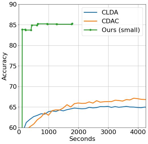
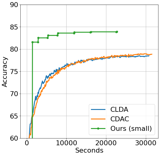
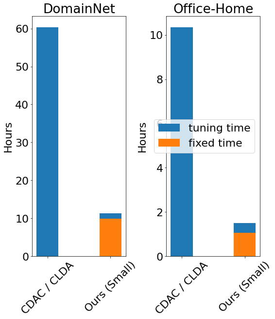
Figure 2: Timing results. (Left) Accuracy over time for 3-shot Art to Clipart on Office-Home. (Center Left) Accuracy over time for 3-shot Real to Clipart on DomainNet. (Center Right) Total time needed to complete all 7 3-shot DomainNet adaptation tasks. (Right) Total time needed to complete all 12 3-shot Office-Home adaptation tasks. Time for our method is divided into inference stage in orange, which only needs to be run once, and training stage in blue, which needs to be tuned. Times are reported on a single P100 GPU.

4.2 Ablation Experiments

We conduct an extensive set of ablation experiments to justify each component of our method.

CORAL and self-training

Table 5 demonstrates the contribution of CORAL and self-training to our method (Steps 1 and 3 in Algorithm 1). Note that CORAL by itself does not consistently improve target accuracy over the naive source classifier. Self-training by itself offers a 1.2% gain on the Office-Home benchmark and a 3.9% gain on the DomainNet benchmark. On both benchmarks, self-training with CORAL achieves higher target accuracy than self-training by itself.

Ensembling

Table 6 shows that the average prediction of the ensemble is almost always better than the best target accuracy of any ensemble member. This result holds regardless of whether all augmentations are used (“full ensemble” in Table 6) or if only one of the augmented datasets is used. This is a powerful result which justifies the additional compute time required for the ensemble. Note that the full 4 $\times$ 7 ensemble achieves better or equal numerical results on all but 3 Office-Home tasks compared to the ensemble with only the non-augmented view. The optimal augmentation varies across tasks, but the full ensemble is able to closely match the best out of 4 target accuracies.

Table 5: CORAL and self-training ablations. No Adaption means training a linear classifier on labeled data only. All experiments use the small ensemble with no augmentations.

Office-Home (3-shot)	R - C	R - P	R - A	P - R	P - C	P - A	A - P	A - C	A - R	C - R	C - A	C - P	Mean
No Adaptation	84.2	94.9	90.0	94.1	82.7	88.9	94.3	82.8	93.7	93.7	89.9	94.3	90.3
CORAL Only	84.4	94.7	89.2	94.0	82.2	88.4	93.9	82.8	93.7	92.9	89.2	93.9	89.9
Self-Training Only	85.7	95.8	91.1	95.4	85.0	89.9	94.8	85.8	94.9	94.8	90.4	94.8	91.5
CORAL + Self-Training	86.1	95.6	90.5	95.4	84.5	90.2	95.5	85.3	95.2	94.9	90.4	95.3	91.6

DomainNet (3-shot)	R $\rightarrow$ C	R $\rightarrow$ P	P $\rightarrow$ C	C $\rightarrow$ S	S $\rightarrow$ P	R $\rightarrow$ S	P $\rightarrow$ R	Mean
No Adaptation	79.0	82.8	80.5	73.7	83.4	70.4	91.9	78.3
CORAL Only	78.7	81.7	78.7	71.8	81.2	71.5	90.5	79.2
Self-Training Only	83.6	84.2	84.6	73.7	84.4	72.2	92.8	82.2
CORAL + Self-Training	84.0	84.7	84.2	75.2	85.1	75.0	92.5	83.0

Table 6: Comparison of augmentations. “Averaged” refers to an ensemble formed by the 7 backbones on the same augmented view.

Office-Home (3-shot)
Augmentation	R - C	R - P	R - A	P - R	P - C	P - A	A - P	A - C	A - R	C - R	C - A	C - P	Mean
Grayscale (Best Member)	82.8	95.2	89.9	94.2	81.2	88.8	94.6	82.8	93.5	93.2	88.8	93.9	89.5
Grayscale (Averaged)	84.0	94.5	90.0	94.5	82.4	89.0	93.8	84.0	94.1	93.9	89.6	94.2	90.3
Perspective (Best Member)	86.1	95.7	90.0	94.7	84.2	89.7	95.1	85.8	94.3	94.3	90.4	94.5	91.0
Perspective (Averaged)	87.5	95.6	90.7	95.0	85.1	90.3	95.1	86.8	94.7	94.7	91.0	95.1	91.8
RandAugment (Best Member)	84.1	95.0	90.3	94.7	82.6	89.2	94.9	83.4	94.1	93.9	89.5	94.5	90.2
RandAugment (Averaged)	86.0	95.5	90.9	95.1	84.5	90.8	95.1	85.3	95.0	95.0	90.1	95.1	91.5
None (Best Member)	85.0	95.8	90.6	94.9	83.2	89.4	95.4	84.1	94.6	94.1	89.6	94.7	90.6
None (Averaged)	86.1	95.6	90.5	95.4	84.5	90.2	95.5	85.3	95.2	94.9	90.4	95.3	91.6
Full Ensemble	87.0	95.7	90.8	95.1	85.0	90.7	95.3	86.3	94.9	94.9	91.2	95.3	91.9

DomainNet (3-shot)
Augmentation	R $\rightarrow$ C	R $\rightarrow$ P	P $\rightarrow$ C	C $\rightarrow$ S	S $\rightarrow$ P	R $\rightarrow$ S	P $\rightarrow$ R	Mean
Grayscale (Best Member)	79.6	82.2	79.5	75.8	83.0	74.4	90.3	80.7
Grayscale (Averaged)	81.3	82.6	81.2	76.0	83.2	75.0	90.6	81.4
Perspective (Best Member)	82.2	84.0	83.1	74.2	84.4	74.1	92.1	81.7
Perspective (Averaged)	83.7	84.3	84.5	74.7	84.8	74.1	92.3	82.6
RandAugment (Best Member)	82.5	83.8	82.8	74.1	83.9	73.3	92.0	81.3
RandAugment (Averaged)	84.1	84.6	84.4	75.2	85.0	74.9	92.5	82.9
None (Best Member)	83.0	84.0	83.0	74.5	84.2	73.9	92.1	81.7
None (Averaged)	84.0	84.7	84.2	75.2	85.1	75.0	92.5	83.0
Full Ensemble	84.2	84.9	84.5	76.0	85.3	75.4	92.5	83.3

5 Limitations

Our work is limited in the following ways: (1) Using a network pre-trained on ImageNet may not work well for certain domain-specific datasets such as synthetic aperture radar, or medical imaging. Furthermore, it would be interesting to perform additional studies on less-curated, in-the-wild datasets using pre-trained models. (2) This work does not consider inference time cost constraints. Inference using an ensemble of large backbones could be impractical in some situations. It would be interesting to investigate using the predictions from our method as pseudo-labels to train a smaller network (e.g. ResNet-34).

6 Conclusion

We propose PACE, a fast and simple Domain Adaptation method, which achieves superior target accuracy on DA benchmarks, while drastically reducing training and tuning time. PACE is built on top of CORAL, self-training, and ensembling, but is to the best of our knowledge the first to investigate a combination of the three methods in a unified framework for both SSDA and UDA.

Broader Impact

The proposed methodology for domain adaptation lowers the computational cost and barrier for entry for ML practitioners while achieving superior DA performance, and thus may be used in novel applications (e.g. edge computing) where computational cost is a concern. DA is important for applications where labels are expensive or difficult to obtain, for example, medical imaging, bioinformatics, self-driving vehicles, languages with few native speakers, and recommendation systems. Also, the ability to work without target labels has the potential to enhance privacy.

Though our work has shown very successful domain transfer results, we note that social biases associated with feature representations require further study to gain an improved understanding of model behavior.

Appendix A Code

Our code is released on GitHub (https://github.com/Chris210634/PACE-Domain-Adaptation). There is no license. Instructions are included with the code. We ran the experiments on a computing cluster with P100 and V100 GPUs. Our job was assigned either a single P100 or V100 GPU depending on availability.

Appendix B Assets Used

We use DomainNet [44] and Office-Home [43] datasets. Some of our code is adapted from [9] (https://github.com/VisionLearningGroup/SSDA_MME). These assets are not licensed.

Appendix C Additional Experimental Results

We include 1-shot SSDA results on Office-Home in Table 7. Very few baselines are listed because most prior work do not publish 1-shot results on Office-Home with the ResNet backbone.

Multi-run Results

We include multi-run results for 3-shot Office-Home, 3-shot DomainNet, and zero-shot Office-Home (UDA) in Table 8, Table 9 and Table 10, respectively. All multi-run results are for the small ensemble on the un-augmented dataset. The standard deviation is with respect to three trials. In the SSDA setting, each trial uses a different random labeled/unlabeled split of the target dataset. in the UDA setting, there is no labeled target data, so the standard deviation is only with respect to randomness in hardware (recall that Algorithm 1 is deterministic).

C.1 Comparison to Domain Adaptation with backbone training

We have constrained our method to training a linear classifier on top of fixed features to reduce the computation required. However, how does this compare to DA with backbone training? Kim et al. [28] experiment with standard UDA methods on three Office-Home adaptation tasks using ConvNeXt-XL and Swin-L backbones pretrained on ImageNet-22k. For ease of comparison, we copy relevant results from Table 4 in [28] into Table 11. In this comparison, our method outperforms the best combination of backbone-adaptation method without training the backbone. This is a promising but preliminary result. We note that the parameters used in [28] may not be optimal, and the exact pretrained backbone used may not be the same as in our study. We also emphasize that we focus on the resource-constrained case and leave any investigation of backbone training to future work.

C.2 Comparison to Bootstrap Aggregation (Bagging)

Bagging is a well-known traditional ensembling method (see Section 14.2 of [42]). In bagging, we make multiple “bootstrapped” copies of the dataset by sampling with replacement, which guarantees that that the copies are not identical. We then run Algorithm 1 on each bootstrapped dataset and return the average prediction. We compare an ensemble formed by 7 bootstrapped datasets to our small ensemble formed by 7 backbones in Table 12. We use the ConvNeXt-XL backbone with $384^{2}$ input resolution and ImageNet-1K fine-tuning for the bagging experiment. From Table 12, observe that an ensemble of bootstrapped datasets performs better than no ensemble at all, but our ensemble of different backbones is clearly better than bagging.

Table 7: SSDA results on Office-Home (1-shot)

Method	R - C	R - P	R - A	P - R	P - C	P - A	A - P	A - C	A - R	C - R	C - A	C - P	Mean
CLDA [14]	60.2	83.2	72.6	81.0	55.9	66.2	76.1	56.3	79.3	76.3	66.3	73.9	70.6
DECOTA [75]	47.2	80.3	64.6	75.5	47.2	56.6	71.1	42.5	73.1	71.0	57.8	72.9	63.3
MCL [76]	67.0	85.5	73.8	81.3	61.1	68.0	79.5	64.4	81.2	78.4	68.5	79.3	74.0
Ours (small)	85.7	95.2	90.0	94.5	82.6	90.2	95.1	84.6	94.3	94.1	90.6	94.9	91.0
Ours (large)	86.2	95.2	90.4	94.7	82.9	90.4	95.2	85.4	94.4	94.3	91.1	94.7	91.2

Table 8: Multi-run results for Office-Home (3-shot). Standard deviation based on 3 trials.

Method	R - C	R - P	R - A	P - R	P - C	P - A	A - P	A - C	A - R	C - R	C - A	C - P	Mean
Ours (small)	85.9$\pm$0.1	95.7$\pm$0.1	90.7$\pm$0.5	94.9$\pm$0.3	84.8$\pm$0.9	90.4$\pm$0.5	95.5$\pm$0.1	85.3$\pm$0.6	94.9$\pm$0.3	94.8$\pm$0.1	90.7$\pm$0.5	95.6$\pm$0.3	91.6$\pm$0.3

Table 9: Multi-run results for DomainNet (3-shot). Standard deviation based on 3 trials.

Method	R $\rightarrow$ C	R $\rightarrow$ P	P $\rightarrow$ C	C $\rightarrow$ S	S $\rightarrow$ P	R $\rightarrow$ S	P $\rightarrow$ R	Mean
Ours (small)	84.1$\pm$0.2	84.6$\pm$0.2	83.7$\pm$0.6	75.0$\pm$0.2	85.1$\pm$0.4	74.4$\pm$0.1	92.2$\pm$0.1	82.7$\pm$0.1

Table 10: Multi-run results for Office-Home (UDA). Standard deviation based on 3 trials.

Method	R - C	R - P	R - A	P - R	P - C	P - A	A - P	A - C	A - R	C - R	C - A	C - P	Mean
Ours (small)	84.4$\pm$0.2	95.1$\pm$0.1	90.0$\pm$0.1	94.8$\pm$0.1	82.7$\pm$0.1	88.9$\pm$0.1	94.1$\pm$0.0	82.5$\pm$0.0	94.4$\pm$0.0	94.3$\pm$0.0	90.2$\pm$0.1	93.5$\pm$0.1	90.4$\pm$0.1

Table 11: Comparison to DA with backbone training [28].

	Backbone	Adaptation	R-A	R-C	R-P	Mean
Numbers from Table 4 in [28]	Swin-L	Source-only	74.3	83.4	90.9	82.8
	ConvNeXt-XL	Source-only	74.0	85.1	91.4	83.5
	Swin-L	DANN [10]	87.3	79.5	93.0	86.6
	ConvNeXt-XL	DANN [10]	87.2	79.8	93.1	86.7
	Swin-L	CDAN [49]	90.1	81.9	93.1	88.4
	ConvNeXt-XL	CDAN [49]	90.2	84.6	93.8	89.5
	Swin-L	AFN [51]	87.4	77.6	92.0	85.7
	ConvNeXt-XL	AFN [51]	86.0	77.7	92.8	85.5
	Swin-L	MDD [13]	87.8	78.0	93.6	86.5
	ConvNeXt-XL	MDD [13]	88.0	77.6	93.6	86.4
	Swin-L	MCC [87]	89.6	81.1	94.1	88.3
	ConvNeXt-XL	MCC [87]	89.5	82.9	94.4	88.9
	Max		90.2	85.1	94.4	89.5
	Ours (small) (Table 2)		89.8	85.0	95.1	90.0
	Ours (large) (Table 2)		90.3	85.7	95.3	90.4

Table 12: Bagging. Comparison of an ensemble formed by 7 bootstrapped datasets to our small ensemble. Only the mean target accuracy for each benchmark is included for brevity. No augmentations are used. 3-shot.

Mean target accuracy	Office-Home	DomainNet
No ensemble (ConvNeXt-XL-384)	90.6	81.7
Our small ensemble (7 members)	91.6	83.0
Bagging (7 bootstrapped datasets)	90.9	81.9

C.3 Projecting Away Domain Direction (PADD)

We introduce PADD as a plug-in alternative to CORAL for domain alignment. PADD finds a linear domain-invariant transformation of the features by iteratively projecting away the “domain direction”. Concretely, for each iteration $t\in 1:T$, we train a binary classifier to discriminate between labeled samples and unlabeled samples. Let $\mathbf{w}\in\mathbb{R}^{d}$, we solve:

$$\mathbf{w}_{t}=\mathop{\text{argmin}}_{\mathbf{w}}\frac{1}{2}\mathop{\mathbb{E}}[\ell_{\text{BCE}}(\sigma(\mathbf{X}_{\text{labeled}}\mathbf{w}),\mathbf{0})]+\frac{1}{2}\mathop{\mathbb{E}}[\ell_{\text{BCE}}(\sigma(\mathbf{X}_{tu}\mathbf{w}),\mathbf{1})]+\lambda_{\text{L1}}\|\mathbf{w}\|_{1}$$ (4)

Similar to the main paper, we optimize Equation 4 over the entire dataset using GD. Here, we run GD for 200 iterations with learning rate 4.0, momentum 0.9, no L2 regularization, L1 regularization $\lambda_{\text{L1}}=0.0002$, and with Nestorov correction. $\ell_{\text{BCE}}$ denotes the binary cross-entropy loss and $\sigma$ denotes the sigmoid function. We then remove the component of the feature vector that points in the direction $\mathbf{w}_{t}$:

$$\begin{split}\mathbf{X}_{\text{labeled}}&=\mathbf{X}_{\text{labeled}}-\text{proj}_{\mathbf{w}_{t}}\mathbf{X}_{\text{labeled}}\\ \mathbf{X}_{tu}&=\mathbf{X}_{tu}-\text{proj}_{\mathbf{w}_{t}}\mathbf{X}_{tu}\end{split}$$ (5)

where $\text{proj}_{\mathbf{w}_{t}}\mathbf{X}$ denotes the projection of the rows of $\mathbf{X}$ onto the vector $\mathbf{w}_{t}$. This process is repeated for $T=30$ iterations. In the end, it is no longer possible to discriminate between labeled and unlabeled data using a linear classifier, i.e. $\mathop{\mathbb{E}}[\sigma(\mathbf{X}_{\text{labeled}}\mathbf{w}_{T})]=\mathop{\mathbb{E}}[\sigma(\mathbf{X}_{tu}\mathbf{w}_{T})]=0.5$. One advantage of PADD is that it is more amenable to mini-batching compared to CORAL; one disadvantage is that PADD may take slightly longer to run. Table 13 shows that PADD attains similar target accuracies as CORAL in our framework.

C.4 Combining Backbone Features without Ensembling

We introduce an alternative method for combining features from different backbones that does not involve ensembling. We first concatenate the features to form one high-dimensional feature vector. We then run the CORAL and self-training steps on the first $k$ principle components of the high-dimensional feature vector. All hyperparameters are the same as the main paper. Results for varying $k$ are presented in Table 14. We make the following observations: (1) There is no clear advantage to setting $k>2048$. (2) This PCA-CORAL-self-training procedure is clearly better than CORAL and self-training on the best backbone (“best ensemble member” in the table). (3) We still obtain better numerical results with the ensembling procedure outlined in the main paper. PCA-CORAL-self-training is faster than training an ensemble.

C.5 Comparison of Different Ensembling Strategies

In the main paper, we consider combining the ensemble predictions by simple averaging. There are more creative ways of combining the predictions, such as majority voting, majority voting weighted by confidence, and majority voting weighted by confidence and validation accuracy. We list results for each of these strategies in Table 15. None of these more creative ensembling strategies are better than simple averaging.

Table 13: Comparison of PADD vs. CORAL with and without self-training. No Adaption means training a linear classifier on labeled data only. All experiments use the small ensemble with no augmentations.

Office-Home (3-shot)	R - C	R - P	R - A	P - R	P - C	P - A	A - P	A - C	A - R	C - R	C - A	C - P	Mean
No Adaptation	84.2	94.9	90.0	94.1	82.7	88.9	94.3	82.8	93.7	93.7	89.9	94.3	90.3
CORAL Only	84.4	94.7	89.2	94.0	82.2	88.4	93.9	82.8	93.7	92.9	89.2	93.9	89.9
PADD Only	85.1	95.2	89.8	94.2	83.5	89.2	94.4	83.4	93.8	93.9	89.7	94.1	90.5
Self-Training Only	85.7	95.8	91.1	95.4	85.0	89.9	94.8	85.8	94.9	94.8	90.4	94.8	91.5
CORAL + Self-Training	86.1	95.6	90.5	95.4	84.5	90.2	95.5	85.3	95.2	94.9	90.4	95.3	91.6
PADD + Self-Training	86.5	95.9	91.1	95.1	85.3	90.1	95.1	85.5	95.0	94.9	90.6	95.5	91.7

DomainNet (3-shot)	R $\rightarrow$ C	R $\rightarrow$ P	P $\rightarrow$ C	C $\rightarrow$ S	S $\rightarrow$ P	R $\rightarrow$ S	P $\rightarrow$ R	Mean
No Adaptation	79.0	82.8	80.5	73.7	83.4	70.4	91.9	78.3
CORAL Only	78.7	81.7	78.7	71.8	81.2	71.5	90.5	79.2
PADD Only	79.4	82.7	80.2	72.7	82.5	71.5	91.6	80.1
Self-Training Only	83.6	84.2	84.6	73.7	84.4	72.2	92.8	82.2
CORAL + Self-Training	84.0	84.7	84.2	75.2	85.1	75.0	92.5	83.0
PADD + Self-Training	84.1	84.5	84.8	74.1	84.2	72.4	92.7	82.4

Table 14: Comparison of PCA-CORAL-self-training with varying $k$ to ensembling.

Office-Home (3-shot) No Augmentation
Method	R - C	R - P	R - A	P - R	P - C	P - A	A - P	A - C	A - R	C - R	C - A	C - P	Mean
Best ensemble member	85.0	95.8	90.6	94.9	83.2	89.4	95.4	84.1	94.6	94.1	89.6	94.7	90.6
PCA, $k=1024$	85.9	95.5	90.3	94.7	84.3	90.5	95.5	84.9	94.8	94.1	89.9	95.1	91.3
PCA, $k=2048$	85.3	95.5	90.2	94.7	84.7	90.6	95.5	84.9	94.7	94.3	90.1	95.1	91.3
PCA, $k=4096$	85.6	95.5	90.2	94.7	84.4	90.1	95.5	84.9	94.9	94.3	89.7	95.0	91.2
Small ensemble	86.1	95.6	90.5	95.4	84.5	90.2	95.5	85.3	95.2	94.9	90.4	95.3	91.6

DomainNet (3-shot) No Augmentation
Method	R $\rightarrow$ C	R $\rightarrow$ P	P $\rightarrow$ C	C $\rightarrow$ S	S $\rightarrow$ P	R $\rightarrow$ S	P $\rightarrow$ R	Mean
Best ensemble member	83.0	84.0	83.0	74.5	84.2	73.9	92.1	81.7
PCA, $k=1024$	83.4	84.2	83.7	75.3	84.7	74.8	92.6	82.7
PCA, $k=2048$	83.7	84.5	84.0	75.6	84.8	75.1	92.5	82.9
PCA, $k=4096$	83.8	84.6	84.0	75.7	84.9	75.1	92.5	82.9
PCA, $k=8192$	83.9	84.6	84.0	75.6	84.7	74.8	92.5	82.9
Small ensemble	84.0	84.7	84.2	75.2	85.1	75.0	92.5	83.0

C.6 Hyperparameter Results

We plot the target accuracy with respect to different hyperparameter settings for 3-shot DomainNet, 1-shot DomainNet, 3-shot Office-Home, 1-shot Office-Home and zero-shot Office-Home in Figures 3, 4, 5, 6 and 7, respectively. The y-axis is target accuracy for all plots. In the SSDA setting, there is a validation set containing 3 labeled samples from each class; in the UDA setting, there is no validation set. We only show results for the Real to Clipart (R $\rightarrow$ C) task. We run 3 trials for each hyperparameter setting and plot the target accuracy of each individual trial as a black dot. We identify 6 degrees of freedom (5 for UDA); in each figure, we vary the hyperparameter choices along one degree of freedom while holding the remaining hyperparameters constant. The default hyperparameters were stated in Section 4: $\eta_{0}=40$, $\eta_{1:T}=80$, $T=30$, $\alpha_{0}=0.4$, $\beta_{0}=0.2$, $\alpha_{1:T}=0.1$, $\beta_{1:T}=0.05$, $\gamma_{1:T}=0.9$, $\tau^{s}_{1:T}=0.8$, $\tau^{tu}_{1:10}=0.9$, $\tau^{tu}_{11:20}=0.8$, $\tau^{tu}_{21:30}=0.7$.

Observations

During the self-training stage, very little weight should be placed on the source data. Our default choices for $\tau^{tu}_{t}$ are close to optimal. Our default choices for the learning rates are close to optimal. Running self-training for more than $T=30$ iterations is unlikely to produce better results. Note that the optimal weights between labeled target data and labeled source data ($\alpha_{0}$ and $\beta_{0}$) depend on the number of labeled samples in each category (Section 6 in [25]). It is not possible to choose a value for $\alpha_{0}$ and $\beta_{0}$ that works well for all settings; prior SSDA methods use $\alpha_{0}=\beta_{0}$.

C.7 Detailed Results on Each Ensemble Member

We list the unlabeled target accuracies for each ensemble member in Tables 16, 17, 18, 19 and 20. The seven ensemble members are listed in the same order as Table 1. In the name of the backbone, “384” and “224” refer to the resolution of the input image; “1K” refers to pretraining on ImageNet-22K and fine-tuning on ImageNet-1K; and “22K” refers to pretraining on ImageNet-22K with no fine-tuning. In these tables, we report both the “Majority vote” and “Averaged” predictions. In majority voting, each ensemble member votes for its own prediction, and the label with the most votes wins. Majority voting is usually worse than simply averaging member predictions, because a confident vote is weighted the same as an unconfident vote. The “Averaged” row in the “No Augmentation” table corresponds to the small ensemble result in the main paper. The “Averaged” row in the “Full Ensemble” table corresponds to the large ensemble result in the main paper.

Table 15: Comparison of different ensembling strategies.

Office-Home (3-shot) Small Ensemble No Augmentation
Method	R - C	R - P	R - A	P - R	P - C	P - A	A - P	A - C	A - R	C - R	C - A	C - P	Mean
Best ensemble member	85.0	95.8	90.6	94.9	83.3	89.7	95.5	84.1	94.7	94.2	89.6	94.7	90.7
Majority vote	86.2	95.6	90.3	95.2	84.5	90.2	95.3	85.1	94.9	94.9	90.2	95.3	91.5
j + Confidence weighting	86.3	95.6	90.5	95.2	84.7	90.5	95.4	85.2	95.0	94.8	90.3	95.2	91.6
j + Validation acc weighting	86.3	95.6	90.5	95.2	84.6	90.5	95.5	85.2	95.0	94.8	90.3	95.2	91.6
Averaged	86.2	95.6	90.5	95.2	84.7	90.5	95.4	85.3	95.1	94.8	90.4	95.2	91.6

Office-Home (3-shot) Large Ensemble
Method	R - C	R - P	R - A	P - R	P - C	P - A	A - P	A - C	A - R	C - R	C - A	C - P	Mean
Best ensemble member	86.1	95.8	90.6	94.9	84.5	89.7	95.5	86.2	94.7	94.2	90.1	94.7	91.4
Majority vote	87.0	95.7	90.7	95.1	85.0	91.0	95.3	86.1	94.9	95.0	91.1	95.3	91.8
j + Confidence weighting	87.1	95.7	90.9	95.3	84.9	91.0	95.3	86.2	94.9	95.0	91.0	95.2	91.9
j + Validation acc weighting	87.1	95.8	90.8	95.3	85.0	91.0	95.3	86.2	94.9	95.0	91.0	95.2	91.9
Averaged	87.0	95.6	90.9	95.3	84.9	90.9	95.4	86.1	95.0	94.9	91.2	95.3	91.9

DomainNet (3-shot) Small Ensemble No Augmentation
Method	R $\rightarrow$ C	R $\rightarrow$ P	P $\rightarrow$ C	C $\rightarrow$ S	S $\rightarrow$ P	R $\rightarrow$ S	P $\rightarrow$ R	Mean
Best ensemble member	83.0	84.1	82.6	74.6	84.3	73.7	92.1	81.8
Majority vote	83.9	84.6	84.0	75.2	84.9	74.6	92.5	82.8
j + Confidence weighting	83.9	84.8	84.1	75.2	84.9	74.9	92.5	82.9
j + Validation acc weighting	84.0	84.8	84.1	75.3	85.0	74.9	92.5	82.9
Averaged	84.0	84.8	84.2	75.3	85.0	75.0	92.5	83.0

DomainNet (3-shot) Large Ensemble
Method	R $\rightarrow$ C	R $\rightarrow$ P	P $\rightarrow$ C	C $\rightarrow$ S	S $\rightarrow$ P	R $\rightarrow$ S	P $\rightarrow$ R	Mean
Best ensemble member	83.0	84.2	83.1	75.2	84.3	74.7	92.1	82.4
Majority vote	84.0	84.9	84.5	75.8	85.2	75.2	92.4	83.2
j + Confidence weighting	84.0	85.1	84.4	75.8	85.2	75.4	92.5	83.2
j + Validation acc weighting	84.0	85.1	84.5	75.9	85.2	75.4	92.5	83.2
Averaged	84.1	85.0	84.5	75.9	85.2	75.4	92.5	83.2

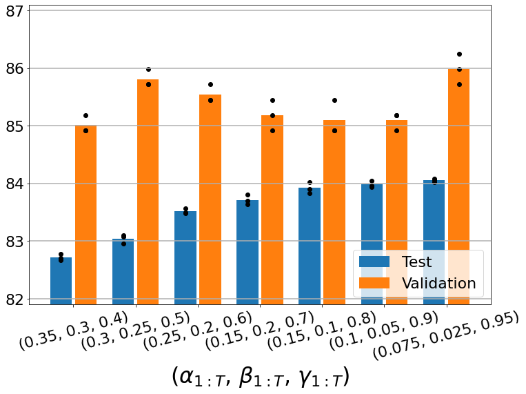
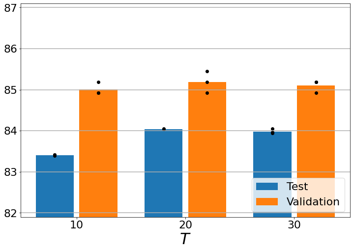
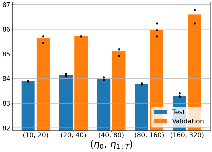
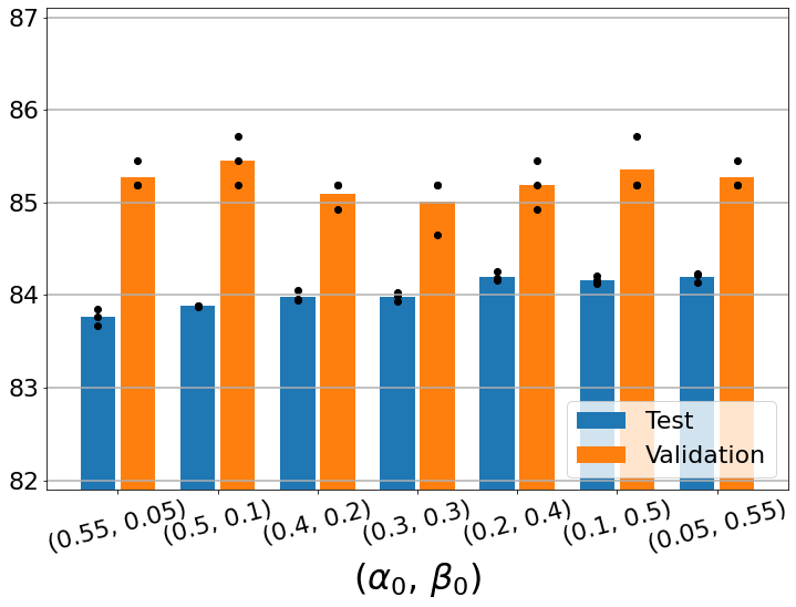
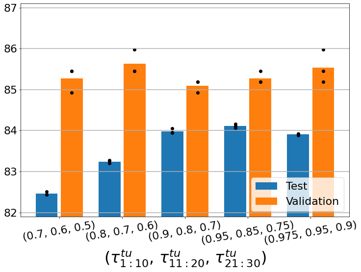
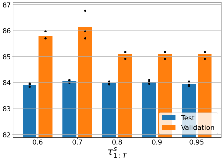
Figure 3: DomainNet 3-shot R to C hyperparameter results.

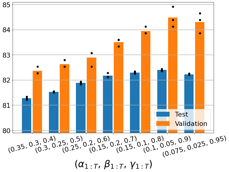
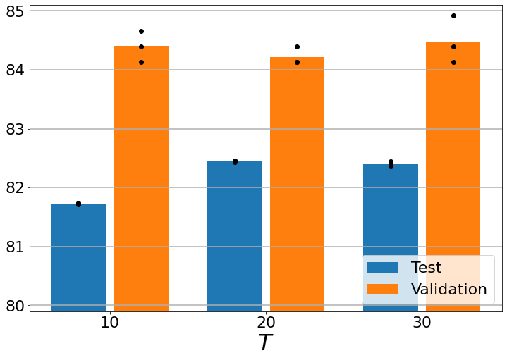
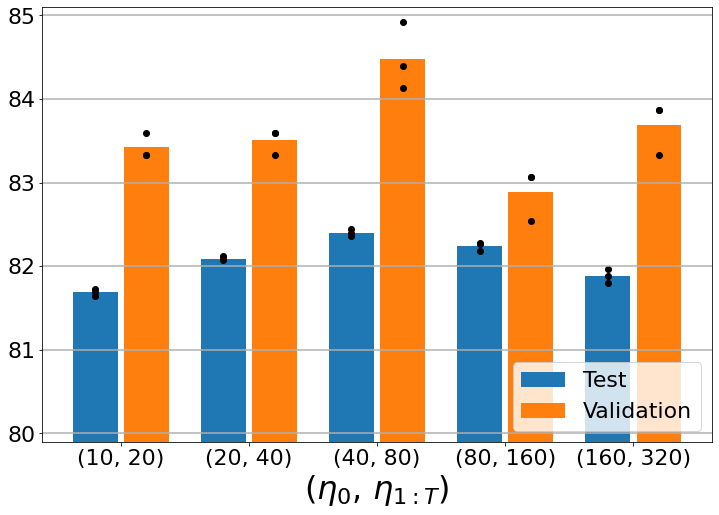
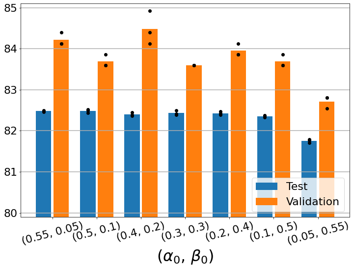
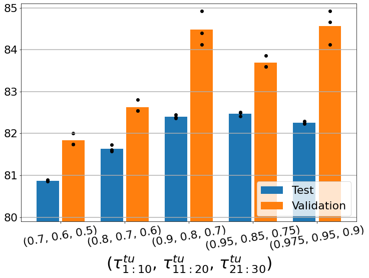
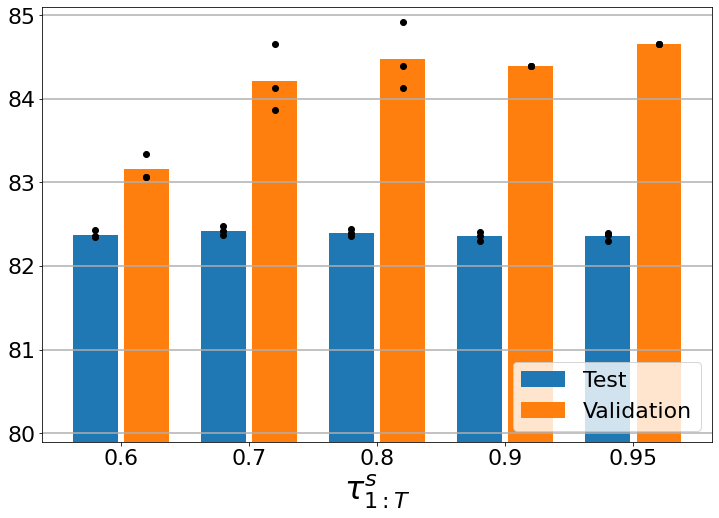
Figure 4: DomainNet 1-shot R to C hyperparameter results.

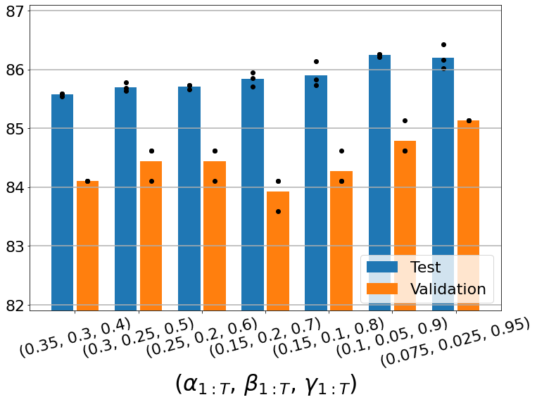
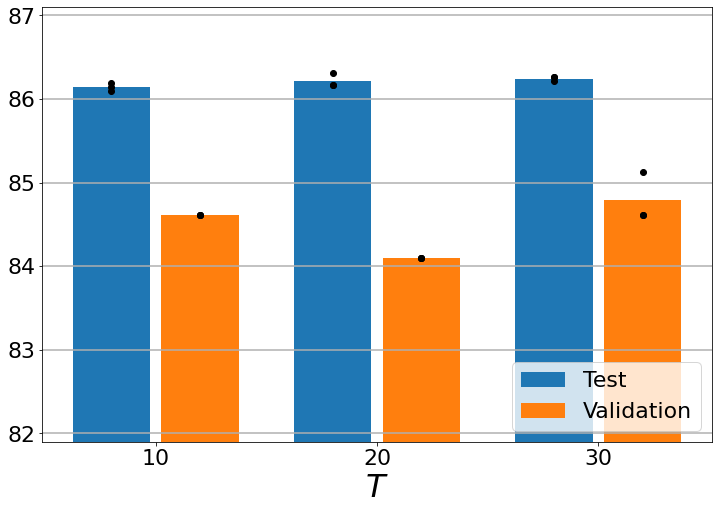
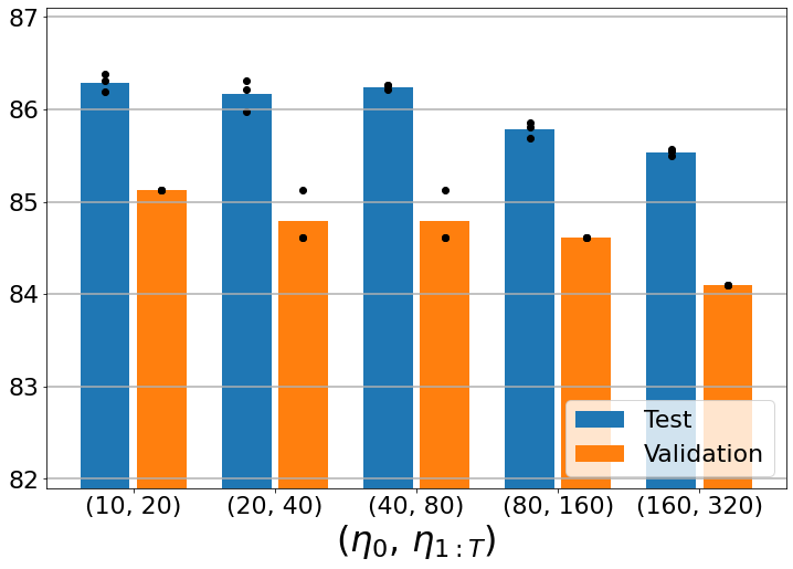
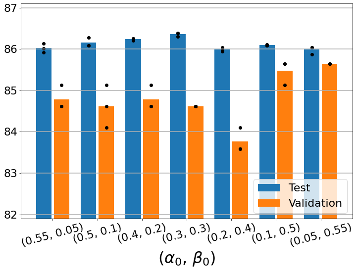
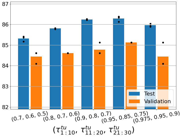
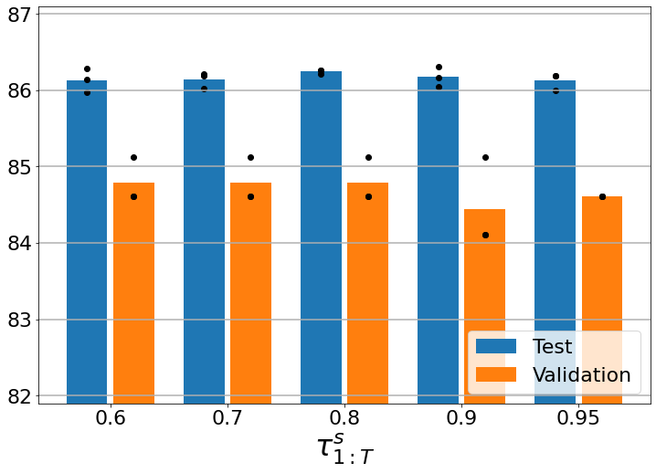
Figure 5: Office-Home 3-shot R to C hyperparameter results.

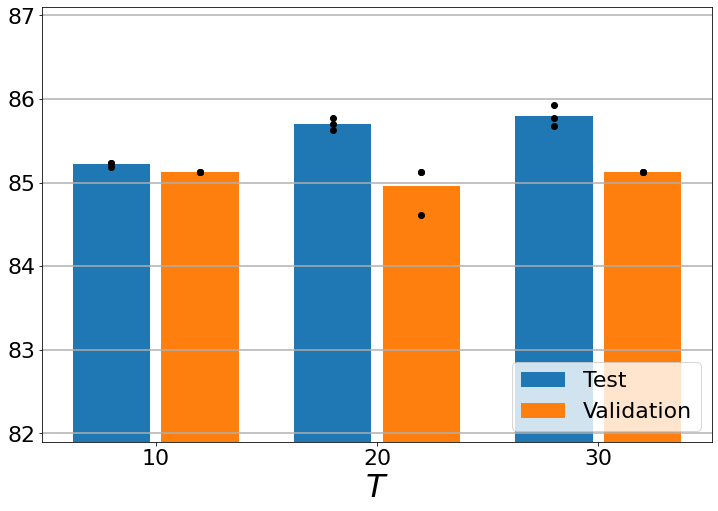
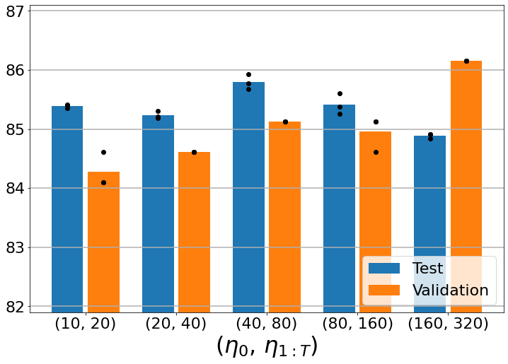
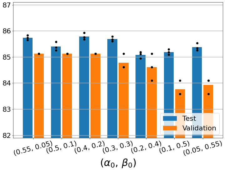
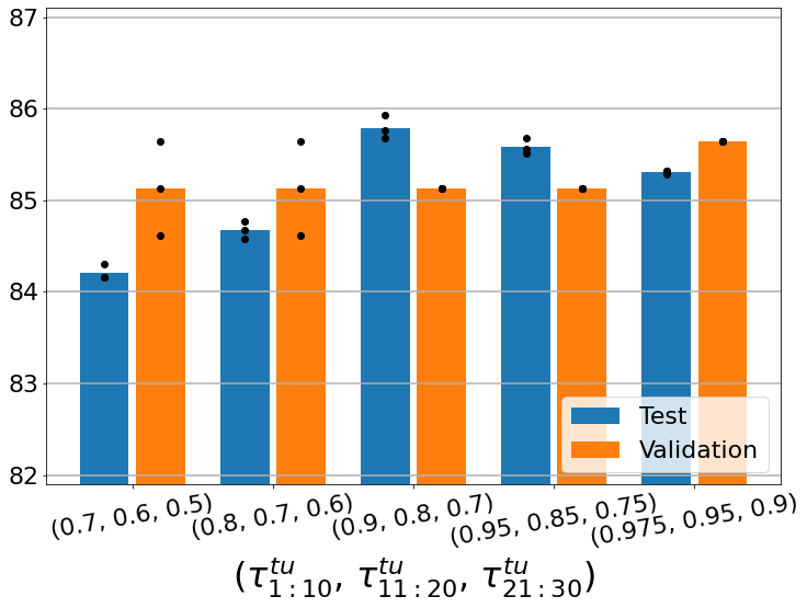
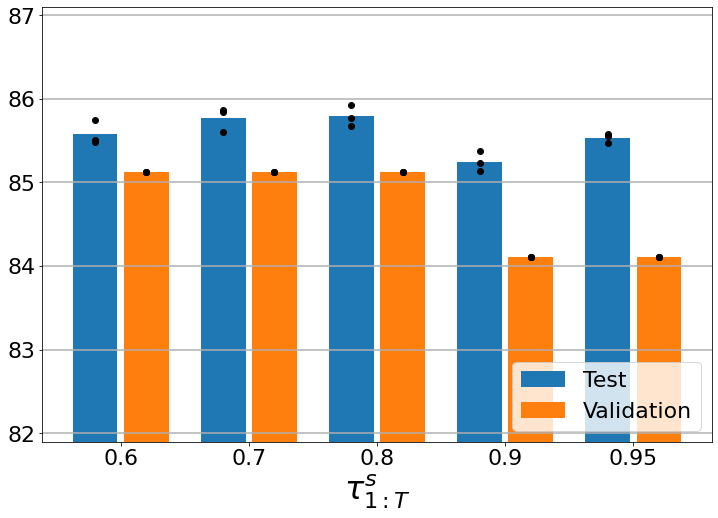
Figure 6: Office-Home 1-shot R to C hyperparameter results.

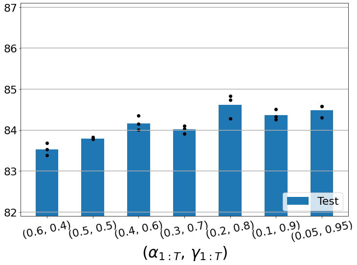
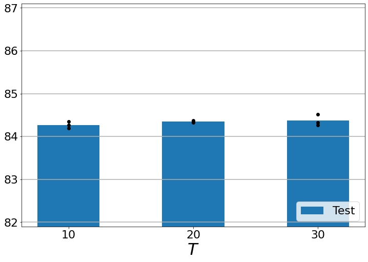
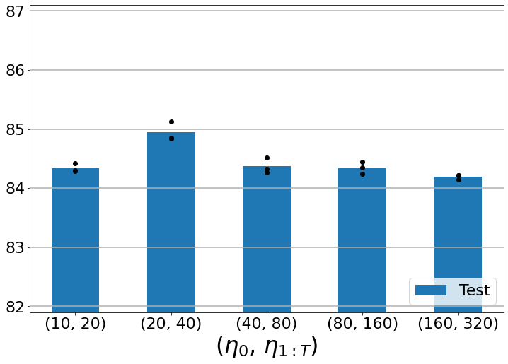
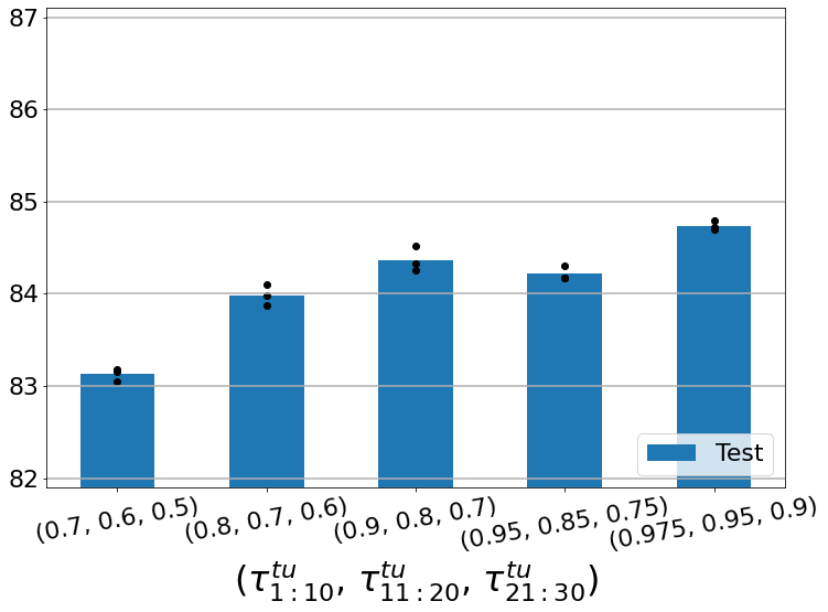
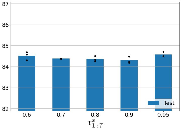
Figure 7: Office-Home zero-shot (UDA) R to C hyperparameter results.

Table 16: Office-Home 3-shot detailed results

Office-Home 3-shot Grayscale
Backbone	R - C	R - P	R - A	P - R	P - C	P - A	A - P	A - C	A - R	C - R	C - A	C - P	Mean
ConvNeXt-384-1K	81.3	95.2	89.9	93.6	80.8	88.8	94.6	81.0	93.4	93.2	88.8	93.9	89.5
ConvNeXt-224-1K	82.8	93.8	88.6	93.7	80.6	86.8	92.9	81.5	93.1	93.0	88.5	93.5	89.1
ConvNeXt-224-22K	81.4	94.2	88.8	94.0	80.8	87.3	93.0	81.4	93.5	92.9	87.5	93.5	89.0
Swin-224-1K	82.3	93.2	86.9	93.6	80.3	85.8	92.3	81.4	92.7	92.4	87.1	92.9	88.4
Swin-224-22K	82.2	93.5	87.4	93.7	79.1	85.3	93.0	81.4	93.2	92.6	86.1	92.0	88.3
Swin-384-1K	82.6	93.6	87.7	93.7	81.0	86.3	93.5	82.5	93.1	93.2	87.0	93.8	89.0
Swin-384-22K	82.5	93.7	88.5	94.2	81.2	87.5	92.8	82.8	93.3	92.7	87.6	92.6	89.1
Max over members	82.8	95.2	89.9	94.2	81.2	88.8	94.6	82.8	93.5	93.2	88.8	93.9	89.5
Majority vote	83.7	94.5	89.5	94.4	82.3	88.9	93.7	83.8	94.0	93.9	89.6	94.3	90.2
Averaged	84.0	94.5	90.0	94.5	82.4	89.0	93.8	84.0	94.1	93.9	89.6	94.2	90.3

Office-Home 3-shot Perspective
Backbone	R - C	R - P	R - A	P - R	P - C	P - A	A - P	A - C	A - R	C - R	C - A	C - P	Mean
ConvNeXt-384-1K	85.2	95.7	90.0	94.4	83.5	89.7	95.1	85.8	94.3	94.1	90.4	94.5	91.0
ConvNeXt-224-1K	85.2	94.8	89.5	93.4	83.5	89.0	94.1	85.7	93.6	93.9	90.1	93.6	90.5
ConvNeXt-224-22K	85.4	95.4	89.1	94.3	84.2	88.5	94.5	85.1	94.1	94.0	89.1	94.4	90.7
Swin-224-1K	84.6	94.6	88.4	93.8	83.9	87.9	93.4	84.7	93.9	93.8	88.0	92.8	90.0
Swin-224-22K	84.8	95.2	88.6	94.1	82.9	88.0	93.9	83.8	94.0	93.5	88.6	93.9	90.1
Swin-384-1K	86.1	95.1	89.3	94.4	84.0	88.8	94.8	85.7	94.2	94.0	89.2	94.4	90.8
Swin-384-22K	85.4	95.3	89.7	94.7	83.1	89.1	94.9	85.3	94.3	94.3	89.6	94.3	90.8
Max over members	86.1	95.7	90.0	94.7	84.2	89.7	95.1	85.8	94.3	94.3	90.4	94.5	91.0
Majority vote	87.4	95.6	90.5	94.9	85.0	90.0	95.2	86.5	94.7	94.8	90.6	95.1	91.7
Averaged	87.5	95.6	90.7	95.0	85.1	90.3	95.1	86.8	94.7	94.7	91.0	95.1	91.8

Office-Home 3-shot RandAugment
Backbone	R - C	R - P	R - A	P - R	P - C	P - A	A - P	A - C	A - R	C - R	C - A	C - P	Mean
ConvNeXt-384-1K	83.0	94.9	90.3	94.4	81.5	89.2	94.9	82.4	93.8	93.2	89.5	94.2	90.1
ConvNeXt-224-1K	83.8	94.6	90.1	93.7	82.6	88.5	93.6	83.3	93.3	93.4	88.2	94.0	89.9
ConvNeXt-224-22K	83.7	94.7	89.0	94.3	81.9	87.9	94.2	82.7	94.1	93.3	87.6	94.3	89.8
Swin-224-1K	82.4	93.9	88.1	94.2	81.4	87.6	94.1	82.0	93.6	93.3	88.2	92.8	89.3
Swin-224-22K	82.6	93.9	87.9	93.6	81.3	87.3	94.1	82.1	93.6	93.1	87.5	92.8	89.2
Swin-384-1K	83.8	94.8	89.0	94.4	82.5	88.8	94.1	83.4	93.9	93.5	89.3	94.5	90.2
Swin-384-22K	84.1	95.0	89.4	94.7	82.5	88.7	94.5	83.3	94.1	93.9	88.2	94.4	90.2
Max over members	84.1	95.0	90.3	94.7	82.6	89.2	94.9	83.4	94.1	93.9	89.5	94.5	90.2
Majority vote	85.9	95.4	90.8	95.1	84.8	90.3	95.1	84.8	94.9	94.9	90.0	95.0	91.4
Averaged	86.0	95.5	90.9	95.1	84.5	90.8	95.1	85.3	95.0	95.0	90.1	95.1	91.5

Office-Home 3-shot No Augmentation
Backbone	R - C	R - P	R - A	P - R	P - C	P - A	A - P	A - C	A - R	C - R	C - A	C - P	Mean
ConvNeXt-384-1K	83.9	95.8	90.6	94.3	82.0	89.3	95.4	83.3	94.3	94.0	89.6	94.7	90.6
ConvNeXt-224-1K	84.1	95.0	89.8	94.2	83.0	88.9	94.6	84.1	94.0	93.7	88.8	94.6	90.4
ConvNeXt-224-22K	84.8	95.5	89.4	94.6	82.4	88.8	95.2	83.3	94.2	93.8	88.3	94.6	90.4
Swin-224-1K	83.2	94.6	88.0	94.5	83.2	88.4	94.2	83.7	94.0	94.1	87.5	93.8	89.9
Swin-224-22K	84.3	95.1	88.0	94.5	82.6	87.8	94.7	82.6	94.6	93.8	88.2	93.8	90.0
Swin-384-1K	84.5	95.0	89.0	94.5	83.0	89.4	94.3	83.7	94.1	94.0	88.4	94.6	90.4
Swin-384-22K	85.0	95.0	89.6	94.9	82.5	89.2	94.6	84.0	94.6	94.1	88.8	94.1	90.5
Max over members	85.0	95.8	90.6	94.9	83.2	89.4	95.4	84.1	94.6	94.1	89.6	94.7	90.6
Majority vote	85.9	95.5	90.3	95.3	84.5	90.3	95.4	85.3	95.1	94.8	90.1	95.3	91.5
Averaged	86.1	95.6	90.5	95.4	84.5	90.2	95.5	85.3	95.2	94.9	90.4	95.3	91.6

Office-Home 3-shot Full Ensemble
Backbone	R - C	R - P	R - A	P - R	P - C	P - A	A - P	A - C	A - R	C - R	C - A	C - P	Mean
Majority vote jjjjjj	86.9	95.7	90.8	95.2	85.0	90.7	95.4	86.1	94.9	94.9	91.3	95.4	91.9
Averaged	87.0	95.7	90.8	95.1	85.0	90.7	95.3	86.3	94.9	94.9	91.2	95.3	91.9

Table 17: DomainNet 3-shot detailed results

DomainNet 3-shot Grayscale
Backbone	R $\rightarrow$ C	R $\rightarrow$ P	P $\rightarrow$ C	C $\rightarrow$ S	S $\rightarrow$ P	R $\rightarrow$ S	P $\rightarrow$ R	Mean
ConvNeXt-384-1K	79.6	82.2	79.3	75.8	83.0	74.4	90.3	80.7
ConvNeXt-224-1K	78.0	80.9	78.5	74.7	80.9	74.2	89.4	79.5
ConvNeXt-224-22K	79.2	80.7	78.3	73.4	80.2	71.9	89.9	79.1
Swin-224-1K	77.8	79.1	77.2	72.5	79.4	71.1	88.8	78.0
Swin-224-22K	77.8	79.7	77.5	71.7	79.7	70.3	89.3	78.0
Swin-384-1K	78.2	80.8	79.3	73.5	81.9	72.8	89.6	79.5
Swin-384-22K	79.5	81.5	79.5	72.8	82.1	72.2	90.2	79.7
Max over members	79.6	82.2	79.5	75.8	83.0	74.4	90.3	80.7
Majority vote	81.1	82.4	80.9	76.0	83.1	74.7	90.6	81.2
Averaged	81.3	82.6	81.2	76.0	83.2	75.0	90.6	81.4

DomainNet 3-shot Perspective
Backbone	R $\rightarrow$ C	R $\rightarrow$ P	P $\rightarrow$ C	C $\rightarrow$ S	S $\rightarrow$ P	R $\rightarrow$ S	P $\rightarrow$ R	Mean
ConvNeXt-384-1K	81.6	84.0	81.7	74.2	84.4	74.1	92.1	81.7
ConvNeXt-224-1K	80.8	82.2	81.2	73.4	82.8	72.8	91.5	80.7
ConvNeXt-224-22K	81.4	82.0	81.9	72.2	81.9	70.8	91.7	80.3
Swin-224-1K	81.0	81.4	81.8	71.0	81.8	69.7	91.0	79.7
Swin-224-22K	81.7	81.9	81.7	70.3	81.4	69.4	91.1	79.7
Swin-384-1K	82.0	82.5	82.4	72.1	83.5	71.9	91.7	80.9
Swin-384-22K	82.2	83.1	83.1	71.9	83.3	71.5	92.0	81.0
Max over members	82.2	84.0	83.1	74.2	84.4	74.1	92.1	81.7
Majority vote	83.4	84.0	84.4	74.6	84.8	73.8	92.3	82.5
Averaged	83.7	84.3	84.5	74.7	84.8	74.1	92.3	82.6

DomainNet 3-shot RandAugment
Backbone	R $\rightarrow$ C	R $\rightarrow$ P	P $\rightarrow$ C	C $\rightarrow$ S	S $\rightarrow$ P	R $\rightarrow$ S	P $\rightarrow$ R	Mean
ConvNeXt-384-1K	80.8	83.8	81.3	74.1	83.9	73.3	92.0	81.3
ConvNeXt-224-1K	80.8	82.1	80.8	73.0	82.4	72.4	91.5	80.4
ConvNeXt-224-22K	81.3	82.1	81.2	71.4	82.0	70.3	91.7	80.0
Swin-224-1K	80.3	81.2	80.4	70.7	81.2	69.9	91.3	79.3
Swin-224-22K	80.9	81.8	80.6	69.6	81.4	69.2	91.4	79.3
Swin-384-1K	82.2	82.9	81.7	72.2	83.3	71.7	91.7	80.8
Swin-384-22K	82.5	83.3	82.8	71.1	83.4	71.4	91.8	80.9
Max over members	82.5	83.8	82.8	74.1	83.9	73.3	92.0	81.3
Majority vote	83.9	84.4	84.2	75.1	84.9	74.5	92.4	82.8
Averaged	84.1	84.6	84.4	75.2	85.0	74.9	92.5	82.9

DomainNet 3-shot No Augmentation
Backbone	R $\rightarrow$ C	R $\rightarrow$ P	P $\rightarrow$ C	C $\rightarrow$ S	S $\rightarrow$ P	R $\rightarrow$ S	P $\rightarrow$ R	Mean
ConvNeXt-384-1K	81.8	84.0	81.6	74.5	84.2	73.9	92.1	81.7
ConvNeXt-224-1K	81.4	82.8	81.4	73.9	83.2	73.0	91.8	81.1
ConvNeXt-224-22K	82.4	82.7	82.1	73.0	82.7	71.2	91.8	80.9
Swin-224-1K	81.5	81.8	81.3	71.9	82.2	71.0	91.5	80.2
Swin-224-22K	81.9	82.5	82.0	71.0	81.9	70.3	91.5	80.2
Swin-384-1K	82.4	83.3	82.6	72.0	84.0	72.6	91.9	81.3
Swin-384-22K	83.0	83.7	83.0	72.4	83.7	72.1	92.0	81.4
Max over members	83.0	84.0	83.0	74.5	84.2	73.9	92.1	81.7
Majority vote	83.9	84.5	84.1	75.1	85.0	74.7	92.5	82.8
Averaged	84.0	84.7	84.2	75.2	85.1	75.0	92.5	83.0

DomainNet 3-shot Full Ensemble
Backbone	R $\rightarrow$ C	R $\rightarrow$ P	P $\rightarrow$ C	C $\rightarrow$ S	S $\rightarrow$ P	R $\rightarrow$ S	P $\rightarrow$ R	Mean
Majority vote jjjjjj	84.1	84.8	84.5	76.0	85.3	75.3	92.5	83.2
Averaged	84.2	84.9	84.5	76.0	85.3	75.4	92.5	83.3

Table 18: Office-Home 1-shot detailed results

Office-Home 1-shot Grayscale
Backbone	R - C	R - P	R - A	P - R	P - C	P - A	A - P	A - C	A - R	C - R	C - A	C - P	Mean
ConvNeXt-384-1K	80.3	94.7	89.2	93.6	78.0	88.4	94.5	79.6	92.8	91.8	89.5	93.9	88.9
ConvNeXt-224-1K	80.2	93.3	88.3	93.9	77.7	87.7	92.4	79.7	92.3	92.5	88.1	92.5	88.2
ConvNeXt-224-22K	79.8	93.6	88.4	93.8	77.7	86.5	92.2	80.5	92.8	92.9	87.0	92.1	88.1
Swin-224-1K	80.0	92.8	86.7	92.7	77.2	86.2	92.2	79.5	92.1	92.7	86.0	91.3	87.4
Swin-224-22K	80.3	93.1	87.0	92.7	75.7	85.7	93.2	79.7	92.1	92.0	85.6	91.5	87.4
Swin-384-1K	81.2	93.5	88.2	93.3	78.8	86.7	92.2	80.1	92.2	93.0	87.5	92.0	88.2
Swin-384-22K	80.9	93.5	88.7	93.0	77.0	86.5	93.0	81.7	92.1	92.5	86.8	91.7	88.1
Max over members	81.2	94.7	89.2	93.9	78.8	88.4	94.5	81.7	92.8	93.0	89.5	93.9	88.9
Majority vote	82.2	94.0	89.1	93.8	79.2	88.8	94.0	82.3	93.2	93.5	89.1	93.0	89.3
Averaged	82.6	94.1	89.2	93.8	79.4	88.8	94.1	82.3	93.3	93.5	89.5	93.3	89.5

Office-Home 1-shot Perspective
Backbone	R - C	R - P	R - A	P - R	P - C	P - A	A - P	A - C	A - R	C - R	C - A	C - P	Mean
ConvNeXt-384-1K	84.3	95.3	90.2	94.1	81.7	89.7	94.8	84.2	93.8	93.7	90.6	94.4	90.6
ConvNeXt-224-1K	84.9	94.4	89.5	93.5	82.0	88.4	93.6	85.0	93.2	93.5	89.6	93.3	90.1
ConvNeXt-224-22K	84.2	95.1	89.0	94.2	81.8	88.2	94.5	84.2	93.6	93.6	89.1	93.1	90.0
Swin-224-1K	85.0	94.8	87.7	93.8	82.2	87.5	93.2	84.5	93.4	92.8	88.2	92.3	89.6
Swin-224-22K	83.7	94.5	88.4	93.6	81.7	87.6	93.6	84.0	93.2	92.8	87.9	92.9	89.5
Swin-384-1K	85.0	94.7	89.1	93.8	83.2	88.4	93.8	86.4	93.4	94.0	89.0	93.0	90.3
Swin-384-22K	85.3	94.0	89.5	94.1	82.2	88.8	93.9	84.7	93.4	93.6	89.5	93.3	90.2
Max over members	85.3	95.3	90.2	94.2	83.2	89.7	94.8	86.4	93.8	94.0	90.6	94.4	90.6
Majority vote	86.4	95.3	90.5	94.4	84.0	90.2	94.7	86.6	94.1	94.4	90.8	94.6	91.3
Averaged	86.8	95.3	90.3	94.5	84.1	90.4	94.8	86.6	94.2	94.4	90.9	94.6	91.4

Office-Home 1-shot RandAugment
Backbone	R - C	R - P	R - A	P - R	P - C	P - A	A - P	A - C	A - R	C - R	C - A	C - P	Mean
ConvNeXt-384-1K	81.1	94.5	89.6	93.9	78.8	89.0	94.0	80.6	93.1	92.7	89.7	93.5	89.2
ConvNeXt-224-1K	82.6	94.1	88.7	93.3	80.2	88.7	93.6	81.9	93.3	92.8	87.7	93.7	89.2
ConvNeXt-224-22K	81.9	94.8	89.0	93.6	80.4	87.3	94.0	82.7	93.0	92.9	88.2	93.6	89.3
Swin-224-1K	81.2	94.2	86.9	93.3	80.2	87.0	93.1	80.7	92.9	92.7	86.6	92.7	88.5
Swin-224-22K	81.1	94.2	87.5	93.9	77.7	87.2	92.9	81.3	93.4	92.1	85.9	92.1	88.3
Swin-384-1K	82.8	94.4	89.0	94.2	81.5	87.8	93.5	83.4	93.1	93.4	89.0	92.6	89.6
Swin-384-22K	82.2	94.1	89.5	93.7	79.1	87.7	94.1	82.2	93.2	93.3	88.0	92.8	89.2
Max over members	82.8	94.8	89.6	94.2	81.5	89.0	94.1	83.4	93.4	93.4	89.7	93.7	89.6
Majority vote	84.7	95.2	90.2	94.6	82.3	90.1	94.8	84.2	94.3	94.1	90.1	94.8	90.8
Averaged	84.8	95.2	90.4	94.6	82.5	90.0	94.8	84.6	94.3	94.2	90.5	94.7	90.9

Office-Home 1-shot No Augmentation
Backbone	R - C	R - P	R - A	P - R	P - C	P - A	A - P	A - C	A - R	C - R	C - A	C - P	Mean
ConvNeXt-384-1K	82.4	95.1	90.5	94.2	79.2	89.6	94.6	82.0	93.5	92.8	90.1	94.1	89.8
ConvNeXt-224-1K	83.2	94.7	89.5	94.0	81.6	88.8	94.4	81.9	93.4	93.5	88.7	94.0	89.8
ConvNeXt-224-22K	82.7	94.7	89.2	94.2	81.5	87.9	94.0	82.1	94.0	93.3	88.9	94.0	89.7
Swin-224-1K	82.2	94.1	88.0	93.7	80.9	88.0	93.6	82.0	93.4	93.8	87.7	93.8	89.3
Swin-224-22K	83.4	94.4	87.6	93.6	79.2	87.5	94.7	81.2	93.5	93.1	87.6	92.4	89.0
Swin-384-1K	83.4	94.5	88.4	94.2	81.4	87.6	94.2	83.3	93.2	93.4	90.1	92.4	89.7
Swin-384-22K	83.3	94.1	89.2	94.0	80.1	88.7	94.6	83.2	93.2	93.1	89.3	93.3	89.7
Max over members	83.4	95.1	90.5	94.2	81.6	89.6	94.7	83.3	94.0	93.8	90.1	94.1	89.8
Majority vote	85.6	95.2	89.9	94.5	82.4	90.0	95.2	84.4	94.3	94.1	90.7	94.8	90.9
Averaged	85.7	95.2	90.0	94.5	82.6	90.2	95.1	84.6	94.3	94.1	90.6	94.9	91.0

Office-Home 1-shot Full Ensemble
Backbone	R - C	R - P	R - A	P - R	P - C	P - A	A - P	A - C	A - R	C - R	C - A	C - P	Mean
Majority vote jjjjjj	86.1	95.2	90.4	94.7	83.0	90.2	95.3	85.1	94.3	94.3	90.9	94.7	91.2
Averaged	86.2	95.2	90.4	94.7	82.9	90.4	95.2	85.4	94.4	94.3	91.1	94.7	91.2

Table 19: DomainNet 1-shot detailed results

DomainNet 1-shot Grayscale
Backbone	R $\rightarrow$ C	R $\rightarrow$ P	P $\rightarrow$ C	C $\rightarrow$ S	S $\rightarrow$ P	R $\rightarrow$ S	P $\rightarrow$ R	Mean
ConvNeXt-384-1K	77.0	82.3	76.4	74.5	82.0	74.1	89.7	79.4
ConvNeXt-224-1K	76.3	80.6	76.6	73.7	80.5	73.3	88.5	78.5
ConvNeXt-224-22K	76.8	80.5	76.1	71.7	80.3	70.9	89.0	77.9
Swin-224-1K	75.7	78.9	74.3	71.3	78.8	70.3	88.1	76.8
Swin-224-22K	76.6	79.0	75.5	70.2	79.1	69.4	88.5	76.9
Swin-384-1K	76.7	80.7	76.7	72.5	81.3	72.2	89.1	78.4
Swin-384-22K	77.3	81.1	77.7	72.0	81.4	70.8	89.4	78.5
Max over members	77.3	82.3	77.7	74.5	82.0	74.1	89.7	79.4
Majority vote	79.0	82.3	78.3	75.0	82.6	74.1	89.5	80.1
Averaged	79.2	82.4	78.5	75.0	82.5	74.3	89.6	80.2

DomainNet 1-shot Perspective
Backbone	R $\rightarrow$ C	R $\rightarrow$ P	P $\rightarrow$ C	C $\rightarrow$ S	S $\rightarrow$ P	R $\rightarrow$ S	P $\rightarrow$ R	Mean
ConvNeXt-384-1K	79.2	83.6	79.9	73.9	84.1	73.0	91.3	80.7
ConvNeXt-224-1K	78.3	81.8	78.9	72.4	81.3	70.9	90.8	79.2
ConvNeXt-224-22K	79.2	81.7	79.3	70.3	81.4	70.0	90.7	78.9
Swin-224-1K	78.9	81.0	79.8	69.6	81.3	69.2	90.7	78.7
Swin-224-22K	79.7	81.4	79.7	68.8	80.9	67.1	90.7	78.3
Swin-384-1K	80.8	82.1	80.8	70.2	82.4	70.6	91.3	79.7
Swin-384-22K	80.9	82.7	80.8	69.5	82.7	69.6	91.2	79.6
Max over members	80.9	83.6	80.8	73.9	84.1	73.0	91.3	80.7
Majority vote	81.3	83.7	82.4	73.2	84.1	72.4	91.6	81.2
Averaged	81.6	83.8	82.5	73.3	84.1	72.7	91.6	81.4

DomainNet 1-shot RandAugment
Backbone	R $\rightarrow$ C	R $\rightarrow$ P	P $\rightarrow$ C	C $\rightarrow$ S	S $\rightarrow$ P	R $\rightarrow$ S	P $\rightarrow$ R	Mean
ConvNeXt-384-1K	78.8	83.1	79.7	73.0	83.5	71.9	91.1	80.2
ConvNeXt-224-1K	78.7	81.8	78.5	72.1	81.6	71.2	90.8	79.2
ConvNeXt-224-22K	79.3	81.6	79.0	69.6	81.7	68.7	90.7	78.7
Swin-224-1K	78.5	80.8	78.9	69.0	80.9	68.1	90.6	78.2
Swin-224-22K	79.5	81.7	78.6	68.0	80.5	66.9	90.5	78.0
Swin-384-1K	80.2	82.3	79.1	70.4	82.4	70.5	91.1	79.4
Swin-384-22K	80.6	83.1	79.9	69.5	82.6	69.0	91.1	79.4
Max over members	80.6	83.1	79.9	73.0	83.5	71.9	91.1	80.2
Majority vote	81.9	84.0	81.8	73.7	84.4	72.5	91.7	81.4
Averaged	82.0	84.3	82.1	73.7	84.3	72.8	91.7	81.5

DomainNet 1-shot No Augmentation
Backbone	R $\rightarrow$ C	R $\rightarrow$ P	P $\rightarrow$ C	C $\rightarrow$ S	S $\rightarrow$ P	R $\rightarrow$ S	P $\rightarrow$ R	Mean
ConvNeXt-384-1K	80.1	83.6	80.0	72.9	84.1	72.2	91.3	80.6
ConvNeXt-224-1K	80.1	82.6	78.7	72.5	82.6	71.7	91.1	79.9
ConvNeXt-224-22K	79.7	82.5	79.2	70.5	81.5	69.6	91.0	79.1
Swin-224-1K	79.7	81.4	79.7	69.9	81.8	69.2	90.9	79.0
Swin-224-22K	80.5	81.9	79.7	68.6	81.1	67.7	90.8	78.6
Swin-384-1K	80.8	82.7	80.6	70.8	83.4	70.8	91.3	80.0
Swin-384-22K	81.4	83.3	80.8	69.9	83.2	69.5	91.3	79.9
Max over members	81.4	83.6	80.8	72.9	84.1	72.2	91.3	80.6
Majority vote	82.2	84.0	82.0	73.5	84.5	72.7	91.7	81.5
Averaged	82.3	84.2	82.2	73.6	84.6	72.8	91.7	81.6

DomainNet 1-shot Full Ensemble
Backbone	R $\rightarrow$ C	R $\rightarrow$ P	P $\rightarrow$ C	C $\rightarrow$ S	S $\rightarrow$ P	R $\rightarrow$ S	P $\rightarrow$ R	Mean
Majority vote jjjjjj	82.2	84.4	82.5	74.6	84.9	74.0	91.7	82.0
Averaged	82.4	84.5	82.6	74.6	84.8	74.0	91.7	82.1

Table 20: Office-Home zero-shot (UDA) detailed results

Office-Home zero-shot (UDA) Grayscale
Backbone	R - C	R - P	R - A	P - R	P - C	P - A	A - P	A - C	A - R	C - R	C - A	C - P	Mean
ConvNeXt-384-1K	79.2	94.5	89.1	93.8	77.9	87.8	93.0	77.9	92.9	92.0	88.3	92.1	88.2
ConvNeXt-224-1K	79.2	92.8	87.8	93.5	78.3	86.1	90.9	77.7	92.8	92.7	87.4	92.2	87.6
ConvNeXt-224-22K	78.8	93.9	88.8	93.5	76.6	85.3	90.8	78.0	92.7	92.2	87.3	91.2	87.4
Swin-224-1K	77.9	92.5	86.3	92.7	76.9	84.1	89.7	77.6	92.0	92.1	85.1	91.1	86.5
Swin-224-22K	78.7	93.2	86.3	92.7	75.4	83.8	90.1	78.2	92.6	92.0	85.4	90.0	86.5
Swin-384-1K	80.3	93.3	86.9	93.6	78.6	84.6	91.1	78.7	92.2	92.6	86.7	90.9	87.5
Swin-384-22K	79.6	92.9	88.0	92.7	76.4	84.8	91.6	79.5	92.4	92.6	86.4	90.2	87.3
Max over members	80.3	94.5	89.1	93.8	78.6	87.8	93.0	79.5	92.9	92.7	88.3	92.2	88.2
Majority vote	81.4	94.2	88.6	93.9	79.5	86.5	92.0	80.5	93.4	93.5	88.3	92.5	88.7
Averaged	81.5	94.2	88.5	93.9	79.7	86.7	92.4	80.7	93.4	93.6	88.7	92.5	88.8

Office-Home zero-shot (UDA) Perspective
Backbone	R - C	R - P	R - A	P - R	P - C	P - A	A - P	A - C	A - R	C - R	C - A	C - P	Mean
ConvNeXt-384-1K	83.6	95.2	89.6	94.5	81.5	88.9	92.7	83.1	93.5	93.5	89.8	94.3	90.0
ConvNeXt-224-1K	83.8	94.4	88.7	93.6	82.0	87.6	93.5	83.6	93.0	93.3	89.1	92.8	89.6
ConvNeXt-224-22K	84.1	94.3	88.7	93.8	80.2	87.6	92.5	83.6	93.3	93.4	88.7	92.6	89.4
Swin-224-1K	84.0	94.7	87.8	93.9	81.6	86.0	91.9	83.6	93.4	93.2	87.6	90.0	89.0
Swin-224-22K	83.0	94.5	88.0	94.0	81.0	86.3	92.4	82.5	93.5	92.4	87.3	91.6	88.9
Swin-384-1K	84.5	94.0	88.2	94.2	82.2	87.7	92.7	84.9	93.8	93.8	88.8	92.8	89.8
Swin-384-22K	83.6	93.8	89.2	94.1	81.1	87.1	92.2	83.9	93.8	93.5	88.8	92.1	89.4
Max over members	84.5	95.2	89.6	94.5	82.2	88.9	93.5	84.9	93.8	93.8	89.8	94.3	90.0
Majority vote	85.7	95.2	89.9	94.6	83.9	88.9	93.6	85.5	94.2	94.3	90.5	93.3	90.8
Averaged	85.9	95.3	89.9	94.8	83.8	88.9	93.8	85.7	94.3	94.4	91.1	93.2	90.9

Office-Home zero-shot (UDA) RandAugment
Backbone	R - C	R - P	R - A	P - R	P - C	P - A	A - P	A - C	A - R	C - R	C - A	C - P	Mean
ConvNeXt-384-1K	80.6	94.8	89.0	94.4	77.9	87.4	93.9	80.0	94.0	92.9	88.5	92.5	88.8
ConvNeXt-224-1K	81.5	93.8	88.7	93.4	79.8	86.6	92.6	80.4	92.9	92.5	88.1	93.4	88.6
ConvNeXt-224-22K	82.1	94.3	88.4	93.6	79.6	87.1	91.9	79.3	93.0	92.8	87.2	93.6	88.6
Swin-224-1K	79.7	93.4	86.9	92.7	78.1	86.2	91.2	79.6	93.1	92.7	86.3	90.4	87.5
Swin-224-22K	80.2	93.7	86.9	93.3	78.3	85.9	92.6	80.3	93.6	92.4	86.7	90.7	87.9
Swin-384-1K	81.1	94.0	88.0	93.9	80.2	86.5	92.4	80.8	93.1	92.9	89.0	91.8	88.6
Swin-384-22K	82.3	93.2	89.0	93.4	79.6	86.5	93.2	80.8	93.7	93.0	87.4	91.9	88.7
Max over members	82.3	94.8	89.0	94.4	80.2	87.4	93.9	80.8	94.0	93.0	89.0	93.6	88.8
Majority vote	84.0	94.7	89.8	94.3	82.4	89.3	94.1	82.7	94.2	94.2	90.2	93.8	90.3
Averaged	84.3	94.9	89.8	94.5	82.4	89.1	94.0	82.9	94.2	94.1	90.4	93.9	90.4

Office-Home zero-shot (UDA) No Augmentation
Backbone	R - C	R - P	R - A	P - R	P - C	P - A	A - P	A - C	A - R	C - R	C - A	C - P	Mean
ConvNeXt-384-1K	81.3	94.6	90.2	94.3	79.4	88.2	92.9	80.9	93.4	92.7	89.3	93.3	89.2
ConvNeXt-224-1K	82.4	94.8	89.1	93.8	81.0	87.6	93.5	79.9	93.6	93.3	88.7	93.4	89.3
ConvNeXt-224-22K	81.6	94.9	89.3	93.9	80.1	87.5	91.8	79.7	93.6	92.7	88.6	93.8	89.0
Swin-224-1K	81.4	93.9	87.4	93.8	80.0	86.5	91.9	80.8	93.6	93.2	87.1	92.0	88.5
Swin-224-22K	82.7	94.3	88.3	93.8	78.5	85.9	91.9	80.5	93.7	93.2	87.7	91.9	88.5
Swin-384-1K	82.7	94.4	87.5	94.2	81.1	88.0	92.8	81.4	93.4	93.3	89.5	92.8	89.3
Swin-384-22K	82.6	93.9	89.2	94.0	78.7	87.5	93.8	81.5	93.7	93.5	89.3	91.9	89.1
Max over members	82.7	94.9	90.2	94.3	81.1	88.2	93.8	81.5	93.7	93.5	89.5	93.8	89.3
Majority vote	85.0	95.1	89.9	94.5	81.9	89.2	94.1	82.3	94.2	94.3	90.4	93.7	90.4
Averaged	85.0	95.1	89.8	94.5	82.0	89.3	94.2	82.5	94.2	94.2	90.3	93.7	90.4

Office-Home zero-shot (UDA) Full Ensemble
Backbone	R - C	R - P	R - A	P - R	P - C	P - A	A - P	A - C	A - R	C - R	C - A	C - P	Mean
Majority vote jjjjjj	85.7	95.2	90.3	94.6	83.0	89.5	93.9	83.5	94.2	94.4	90.6	93.4	90.7
Averaged	85.7	95.3	90.3	94.6	83.0	89.6	94.0	84.0	94.3	94.4	90.7	93.6	90.8

References

- [1] Sicheng Zhao, Xiangyu Yue, Shanghang Zhang, Bo Li, Han Zhao, Bichen Wu, Ravi Krishna, Joseph E Gonzalez, Alberto L Sangiovanni-Vincentelli, Sanjit A Seshia, et al. A review of single-source deep unsupervised visual domain adaptation. IEEE Transactions on Neural Networks and Learning Systems, 2020.
- [2] Yifan Zhang, Shuaicheng Niu, Zhen Qiu, Ying Wei, Peilin Zhao, Jianhua Yao, Junzhou Huang, Qingyao Wu, and Mingkui Tan. Covid-da: deep domain adaptation from typical pneumonia to covid-19. arXiv preprint arXiv:2005.01577, 2020.
- [3] Linda Wang, Zhong Qiu Lin, and Alexander Wong. Covid-net: A tailored deep convolutional neural network design for detection of covid-19 cases from chest x-ray images. Scientific Reports, 10(1):1–12, 2020.
- [4] Longlong Jing and Yingli Tian. Self-supervised visual feature learning with deep neural networks: A survey. IEEE transactions on pattern analysis and machine intelligence, 43(11):4037–4058, 2020.
- [5] Ashish Jaiswal, Ashwin Ramesh Babu, Mohammad Zaki Zadeh, Debapriya Banerjee, and Fillia Makedon. A survey on contrastive self-supervised learning. Technologies, 9(1):2, 2020.
- [6] Jesper E Van Engelen and Holger H Hoos. A survey on semi-supervised learning. Machine Learning, 109(2):373–440, 2020.
- [7] Fuzhen Zhuang, Zhiyuan Qi, Keyu Duan, Dongbo Xi, Yongchun Zhu, Hengshu Zhu, Hui Xiong, and Qing He. A comprehensive survey on transfer learning. Proceedings of the IEEE, 109(1):43–76, 2020.
- [8] Garrett Wilson and Diane J Cook. A survey of unsupervised deep domain adaptation. ACM Transactions on Intelligent Systems and Technology (TIST), 11(5):1–46, 2020.
- [9] Kuniaki Saito, Donghyun Kim, Stan Sclaroff, Trevor Darrell, and Kate Saenko. Semi-supervised domain adaptation via minimax entropy. In Proceedings of the IEEE/CVF International Conference on Computer Vision, pages 8050–8058, 2019.
- [10] Yaroslav Ganin, Evgeniya Ustinova, Hana Ajakan, Pascal Germain, Hugo Larochelle, François Laviolette, Mario Marchand, and Victor Lempitsky. Domain-adversarial training of neural networks. The journal of machine learning research, 17(1):2096–2030, 2016.
- [11] David Acuna, Guojun Zhang, Marc T Law, and Sanja Fidler. f-domain adversarial learning: Theory and algorithms. In International Conference on Machine Learning, pages 66–75. PMLR, 2021.
- [12] Hong Liu, Jianmin Wang, and Mingsheng Long. Cycle self-training for domain adaptation. Advances in Neural Information Processing Systems, 34, 2021.
- [13] Yuchen Zhang, Tianle Liu, Mingsheng Long, and Michael Jordan. Bridging theory and algorithm for domain adaptation. In International Conference on Machine Learning, pages 7404–7413. PMLR, 2019.
- [14] Ankit Singh. Clda: Contrastive learning for semi-supervised domain adaptation. Advances in Neural Information Processing Systems, 34, 2021.
- [15] Jichang Li, Guanbin Li, Yemin Shi, and Yizhou Yu. Cross-domain adaptive clustering for semi-supervised domain adaptation. In Proceedings of the IEEE/CVF Conference on Computer Vision and Pattern Recognition, pages 2505–2514, 2021.
- [16] Yixin Zhang, Junjie Li, and Zilei Wang. Low-confidence samples matter for domain adaptation. arXiv preprint arXiv:2202.02802, 2022.
- [17] Taekyung Kim and Changick Kim. Attract, perturb, and explore: Learning a feature alignment network for semi-supervised domain adaptation. In European conference on computer vision, pages 591–607. Springer, 2020.
- [18] Ze Liu, Yutong Lin, Yue Cao, Han Hu, Yixuan Wei, Zheng Zhang, Stephen Lin, and Baining Guo. Swin transformer: Hierarchical vision transformer using shifted windows. In Proceedings of the IEEE/CVF International Conference on Computer Vision, pages 10012–10022, 2021.
- [19] Zhuang Liu, Hanzi Mao, Chao-Yuan Wu, Christoph Feichtenhofer, Trevor Darrell, and Saining Xie. A convnet for the 2020s. arXiv preprint arXiv:2201.03545, 2022.
- [20] Yue Wang, Ziyu Jiang, Xiaohan Chen, Pengfei Xu, Yang Zhao, Yingyan Lin, and Zhangyang Wang. E2-train: Training state-of-the-art cnns with over 80% energy savings. Advances in Neural Information Processing Systems, 32, 2019.
- [21] Chaoyang He, Murali Annavaram, and Salman Avestimehr. Group knowledge transfer: Federated learning of large cnns at the edge. Advances in Neural Information Processing Systems, 33:14068–14080, 2020.
- [22] David Berthelot, Rebecca Roelofs, Kihyuk Sohn, Nicholas Carlini, and Alex Kurakin. Adamatch: A unified approach to semi-supervised learning and domain adaptation. arXiv preprint arXiv:2106.04732, 2021.
- [23] Jia Deng, Wei Dong, Richard Socher, Li-Jia Li, Kai Li, and Li Fei-Fei. Imagenet: A large-scale hierarchical image database. In 2009 IEEE conference on computer vision and pattern recognition, pages 248–255. Ieee, 2009.
- [24] Baochen Sun, Jiashi Feng, and Kate Saenko. Return of frustratingly easy domain adaptation. In AAAI, 2016.
- [25] Shai Ben-David, John Blitzer, Koby Crammer, Alex Kulesza, Fernando Pereira, and Jennifer Wortman Vaughan. A theory of learning from different domains. Machine learning, 79(1):151–175, 2010.
- [26] Kuniaki Saito, Kohei Watanabe, Yoshitaka Ushiku, and Tatsuya Harada. Maximum classifier discrepancy for unsupervised domain adaptation. In Proceedings of the IEEE conference on computer vision and pattern recognition, pages 3723–3732, 2018.
- [27] Guoliang Kang, Lu Jiang, Yi Yang, and Alexander G Hauptmann. Contrastive adaptation network for unsupervised domain adaptation. In Proceedings of the IEEE/CVF Conference on Computer Vision and Pattern Recognition, pages 4893–4902, 2019.
- [28] Donghyun Kim, Kaihong Wang, Stan Sclaroff, and Kate Saenko. A broad study of pre-training for domain generalization and adaptation. arXiv preprint arXiv:2203.11819, 2022.
- [29] Zirui Wang, Zihang Dai, Barnabás Póczos, and Jaime Carbonell. Characterizing and avoiding negative transfer. In Proceedings of the IEEE/CVF Conference on Computer Vision and Pattern Recognition, pages 11293–11302, 2019.
- [30] Dong-Hyun Lee et al. Pseudo-label: The simple and efficient semi-supervised learning method for deep neural networks. In Workshop on challenges in representation learning, ICML, volume 3, page 896, 2013.
- [31] Kihyuk Sohn, David Berthelot, Nicholas Carlini, Zizhao Zhang, Han Zhang, Colin A Raffel, Ekin Dogus Cubuk, Alexey Kurakin, and Chun-Liang Li. Fixmatch: Simplifying semi-supervised learning with consistency and confidence. Advances in Neural Information Processing Systems, 33:596–608, 2020.
- [32] Eric Arazo, Diego Ortego, Paul Albert, Noel E O’Connor, and Kevin McGuinness. Pseudo-labeling and confirmation bias in deep semi-supervised learning. In 2020 International Joint Conference on Neural Networks (IJCNN), pages 1–8. IEEE, 2020.
- [33] Hieu Pham, Zihang Dai, Qizhe Xie, and Quoc V Le. Meta pseudo labels. In Proceedings of the IEEE/CVF Conference on Computer Vision and Pattern Recognition, pages 11557–11568, 2021.
- [34] Baixu Chen, Junguang Jiang, Ximei Wang, Jianmin Wang, and Mingsheng Long. Debiased pseudo labeling in self-training. arXiv preprint arXiv:2202.07136, 2022.
- [35] Hammam Alshazly, Christoph Linse, Erhardt Barth, and Thomas Martinetz. Ensembles of deep learning models and transfer learning for ear recognition. Sensors, 19(19):4139, 2019.
- [36] Safa Alsafari, Samira Sadaoui, and Malek Mouhoub. Deep learning ensembles for hate speech detection. In 2020 IEEE 32nd International Conference on Tools with Artificial Intelligence (ICTAI), pages 526–531. IEEE, 2020.
- [37] Sivaramakrishnan Rajaraman, Jenifer Siegelman, Philip O Alderson, Lucas S Folio, Les R Folio, and Sameer K Antani. Iteratively pruned deep learning ensembles for covid-19 detection in chest x-rays. Ieee Access, 8:115041–115050, 2020.
- [38] Kaiyang Zhou, Yongxin Yang, Yu Qiao, and Tao Xiang. Domain adaptive ensemble learning. IEEE Transactions on Image Processing, 30:8008–8018, 2021.
- [39] Guoliang Kang, Lu Jiang, Yunchao Wei, Yi Yang, and Alexander G Hauptmann. Contrastive adaptation network for single-and multi-source domain adaptation. IEEE transactions on pattern analysis and machine intelligence, 2020.
- [40] Viraj Prabhu, Shivam Khare, Deeksha Kartik, and Judy Hoffman. Sentry: Selective entropy optimization via committee consistency for unsupervised domain adaptation. In Proceedings of the IEEE/CVF International Conference on Computer Vision, pages 8558–8567, 2021.
- [41] Ross Wightman. Pytorch image models. https://github.com/rwightman/pytorch-image-models, 2019.
- [42] Christopher M Bishop and Nasser M Nasrabadi. Pattern recognition and machine learning, volume 4. Springer, 2006.
- [43] Hemanth Venkateswara, Jose Eusebio, Shayok Chakraborty, and Sethuraman Panchanathan. Deep hashing network for unsupervised domain adaptation. In Proceedings of the IEEE Conference on Computer Vision and Pattern Recognition, pages 5018–5027, 2017.
- [44] Xingchao Peng, Qinxun Bai, Xide Xia, Zijun Huang, Kate Saenko, and Bo Wang. Moment matching for multi-source domain adaptation. In Proceedings of the IEEE International Conference on Computer Vision, pages 1406–1415, 2019.
- [45] Kaiming He, Xiangyu Zhang, Shaoqing Ren, and Jian Sun. Deep residual learning for image recognition. In Proceedings of the IEEE conference on computer vision and pattern recognition, pages 770–778, 2016.
- [46] Hugo Touvron, Matthieu Cord, Matthijs Douze, Francisco Massa, Alexandre Sablayrolles, and Hervé Jégou. Training data-efficient image transformers & distillation through attention. In International Conference on Machine Learning, pages 10347–10357. PMLR, 2021.
- [47] Alexey Dosovitskiy, Lucas Beyer, Alexander Kolesnikov, Dirk Weissenborn, Xiaohua Zhai, Thomas Unterthiner, Mostafa Dehghani, Matthias Minderer, Georg Heigold, Sylvain Gelly, et al. An image is worth 16x16 words: Transformers for image recognition at scale. arXiv preprint arXiv:2010.11929, 2020.
- [48] Mingsheng Long, Han Zhu, Jianmin Wang, and Michael I Jordan. Deep transfer learning with joint adaptation networks. In International conference on machine learning, pages 2208–2217. PMLR, 2017.
- [49] Mingsheng Long, Zhangjie Cao, Jianmin Wang, and Michael I Jordan. Conditional adversarial domain adaptation. Advances in neural information processing systems, 31, 2018.
- [50] Minghao Chen, Shuai Zhao, Haifeng Liu, and Deng Cai. Adversarial-learned loss for domain adaptation. In Proceedings of the AAAI Conference on Artificial Intelligence, volume 34, pages 3521–3528, 2020.
- [51] Ruijia Xu, Guanbin Li, Jihan Yang, and Liang Lin. Larger norm more transferable: An adaptive feature norm approach for unsupervised domain adaptation. In Proceedings of the IEEE/CVF International Conference on Computer Vision, pages 1426–1435, 2019.
- [52] Yabin Zhang, Hui Tang, Kui Jia, and Mingkui Tan. Domain-symmetric networks for adversarial domain adaptation. In Proceedings of the IEEE/CVF Conference on Computer Vision and Pattern Recognition, pages 5031–5040, 2019.
- [53] Ximei Wang, Liang Li, Weirui Ye, Mingsheng Long, and Jianmin Wang. Transferable attention for domain adaptation. In Proceedings of the AAAI Conference on Artificial Intelligence, volume 33, pages 5345–5352, 2019.
- [54] Shuhao Cui, Shuhui Wang, Junbao Zhuo, Liang Li, Qingming Huang, and Qi Tian. Towards discriminability and diversity: Batch nuclear-norm maximization under label insufficient situations. In Proceedings of the IEEE/CVF Conference on Computer Vision and Pattern Recognition, pages 3941–3950, 2020.
- [55] Xiang Jiang, Qicheng Lao, Stan Matwin, and Mohammad Havaei. Implicit class-conditioned domain alignment for unsupervised domain adaptation. In International Conference on Machine Learning, pages 4816–4827. PMLR, 2020.
- [56] Vinod Kumar Kurmi, Shanu Kumar, and Vinay P Namboodiri. Attending to discriminative certainty for domain adaptation. In Proceedings of the IEEE/CVF Conference on Computer Vision and Pattern Recognition, pages 491–500, 2019.
- [57] Lanqing Hu, Meina Kan, Shiguang Shan, and Xilin Chen. Unsupervised domain adaptation with hierarchical gradient synchronization. In Proceedings of the IEEE/CVF Conference on Computer Vision and Pattern Recognition, pages 4043–4052, 2020.
- [58] Shuhao Cui, Shuhui Wang, Junbao Zhuo, Chi Su, Qingming Huang, and Qi Tian. Gradually vanishing bridge for adversarial domain adaptation. In Proceedings of the IEEE/CVF conference on computer vision and pattern recognition, pages 12455–12464, 2020.
- [59] Shuang Li, Chi Liu, Qiuxia Lin, Binhui Xie, Zhengming Ding, Gao Huang, and Jian Tang. Domain conditioned adaptation network. In Proceedings of the AAAI Conference on Artificial Intelligence, volume 34, pages 11386–11393, 2020.
- [60] Zhongqi Yue, Qianru Sun, Xian-Sheng Hua, and Hanwang Zhang. Transporting causal mechanisms for unsupervised domain adaptation. In Proceedings of the IEEE/CVF International Conference on Computer Vision, pages 8599–8608, 2021.
- [61] Shuhao Cui, Xuan Jin, Shuhui Wang, Yuan He, and Qingming Huang. Heuristic domain adaptation. Advances in Neural Information Processing Systems, 33:7571–7583, 2020.
- [62] Guoqiang Wei, Cuiling Lan, Wenjun Zeng, and Zhibo Chen. Metaalign: Coordinating domain alignment and classification for unsupervised domain adaptation. In Proceedings of the IEEE/CVF Conference on Computer Vision and Pattern Recognition, pages 16643–16653, 2021.
- [63] Guoqiang Wei, Cuiling Lan, Wenjun Zeng, Zhizheng Zhang, and Zhibo Chen. Toalign: Task-oriented alignment for unsupervised domain adaptation. Advances in Neural Information Processing Systems, 34, 2021.
- [64] Jaemin Na, Heechul Jung, Hyung Jin Chang, and Wonjun Hwang. Fixbi: Bridging domain spaces for unsupervised domain adaptation. In Proceedings of the IEEE/CVF Conference on Computer Vision and Pattern Recognition, pages 1094–1103, 2021.
- [65] Shuang Li, Mixue Xie, Fangrui Lv, Chi Harold Liu, Jian Liang, Chen Qin, and Wei Li. Semantic concentration for domain adaptation. In Proceedings of the IEEE/CVF International Conference on Computer Vision, pages 9102–9111, 2021.
- [66] Jian Liang, Dapeng Hu, and Jiashi Feng. Domain adaptation with auxiliary target domain-oriented classifier. In Proceedings of the IEEE/CVF Conference on Computer Vision and Pattern Recognition, pages 16632–16642, 2021.
- [67] Junjie Li, Yixin Zhang, Zilei Wang, and Keyu Tu. Semantic-aware representation learning via probability contrastive loss. arXiv preprint arXiv:2111.06021, 2021.
- [68] Wenxuan Ma, Jinming Zhang, Shuang Li, Chi Harold Liu, Yulin Wang, and Wei Li. Exploiting both domain-specific and invariant knowledge via a win-win transformer for unsupervised domain adaptation. arXiv preprint arXiv:2111.12941, 2021.
- [69] Tongkun Xu, Weihua Chen, Pichao Wang, Fan Wang, Hao Li, and Rong Jin. Cdtrans: Cross-domain transformer for unsupervised domain adaptation. arXiv preprint arXiv:2109.06165, 2021.
- [70] Jinyu Yang, Jingjing Liu, Ning Xu, and Junzhou Huang. Tvt: Transferable vision transformer for unsupervised domain adaptation. arXiv preprint arXiv:2108.05988, 2021.
- [71] Tao Sun, Cheng Lu, Tianshuo Zhang, and Haibin Ling. Safe self-refinement for transformer-based domain adaptation. In Proceedings of the IEEE/CVF Conference on Computer Vision and Pattern Recognition (CVPR), 2022.
- [72] Xiyu Wang, Pengxin Guo, and Yu Zhang. Domain adaptation via bidirectional cross-attention transformer. arXiv preprint arXiv:2201.05887, 2022.
- [73] Da Li and Timothy Hospedales. Online meta-learning for multi-source and semi-supervised domain adaptation. In European Conference on Computer Vision, pages 382–403. Springer, 2020.
- [74] Jiaxing Huang, Dayan Guan, Aoran Xiao, and Shijian Lu. Semi-supervised domain adaptation via adaptive and progressive feature alignment. arXiv preprint arXiv:2106.02845, 2021.
- [75] Luyu Yang, Yan Wang, Mingfei Gao, Abhinav Shrivastava, Kilian Q Weinberger, Wei-Lun Chao, and Ser-Nam Lim. Deep co-training with task decomposition for semi-supervised domain adaptation. In Proceedings of the IEEE/CVF International Conference on Computer Vision, pages 8906–8916, 2021.
- [76] Zizheng Yan, Yushuang Wu, Guanbin Li, Yipeng Qin, Xiaoguang Han, and Shuguang Cui. Multi-level consistency learning for semi-supervised domain adaptation. arXiv preprint arXiv:2205.04066, 2022.
- [77] Pin Jiang, Aming Wu, Yahong Han, Yunfeng Shao, Meiyu Qi, and Bingshuai Li. Bidirectional adversarial training for semi-supervised domain adaptation. In IJCAI, pages 934–940, 2020.
- [78] Can Qin, Lichen Wang, Qianqian Ma, Yu Yin, Huan Wang, and Yun Fu. Contradictory structure learning for semi-supervised domain adaptation. In Proceedings of the 2021 SIAM International Conference on Data Mining (SDM), pages 576–584. SIAM, 2021.
- [79] Liang Li, Aming Wu, and Yahong Han. Graph-in-graph contrastive learning for semi-supervised adaptation. In 2021 IEEE International Conference on Multimedia and Expo (ICME), pages 1–6. IEEE, 2021.
- [80] Manuel Pérez-Carrasco, Pavlos Protopapas, and Guillermo Cabrera-Vives. Con2da: Simplifying semi-supervised domain adaptation by learning consistent and contrastive feature representations. arXiv preprint arXiv:2204.01558, 2022.
- [81] Jeongbeen Yoon, Dahyun Kang, and Minsu Cho. Semi-supervised domain adaptation via sample-to-sample self-distillation. In Proceedings of the IEEE/CVF Winter Conference on Applications of Computer Vision, pages 1978–1987, 2022.
- [82] Yu Zhang, Gongbo Liang, and Nathan Jacobs. Dynamic feature alignment for semi-supervised domain adaptation. In British Machine Vision Conference (BMVC), 2021.
- [83] Anurag Singh, Naren Doraiswamy, Sawa Takamuku, Megh Bhalerao, Titir Dutta, Soma Biswas, Aditya Chepuri, Balasubramanian Vengatesan, and Naotake Natori. Improving semi-supervised domain adaptation using effective target selection and semantics. In Proceedings of the IEEE/CVF Conference on Computer Vision and Pattern Recognition, pages 2709–2718, 2021.
- [84] Samarth Mishra, Kate Saenko, and Venkatesh Saligrama. Surprisingly simple semi-supervised domain adaptation with pretraining and consistency. arXiv preprint arXiv:2101.12727, 2021.
- [85] Kai Li, Chang Liu, Handong Zhao, Yulun Zhang, and Yun Fu. Ecacl: A holistic framework for semi-supervised domain adaptation. In Proceedings of the IEEE/CVF International Conference on Computer Vision, pages 8578–8587, 2021.
- [86] Ekin D Cubuk, Barret Zoph, Jonathon Shlens, and Quoc V Le. Randaugment: Practical automated data augmentation with a reduced search space. In Proceedings of the IEEE/CVF Conference on Computer Vision and Pattern Recognition Workshops, pages 702–703, 2020.
- [87] Ying Jin, Ximei Wang, Mingsheng Long, and Jianmin Wang. Minimum class confusion for versatile domain adaptation. In European Conference on Computer Vision, pages 464–480. Springer, 2020.