Censored Quantile Regression Neural Networks
for Distribution-Free Survival Analysis

Abstract

This paper considers doing quantile regression on censored data using neural networks (NNs). This adds to the survival analysis toolkit by allowing direct prediction of the target variable, along with a distribution-free characterisation of uncertainty, using a flexible function approximator. We begin by showing how an algorithm popular in linear models can be applied to NNs. However, the resulting procedure is inefficient, requiring sequential optimisation of an individual NN at each desired quantile. Our major contribution is a novel algorithm that simultaneously optimises a grid of quantiles output by a single NN. To offer theoretical insight into our algorithm, we show firstly that it can be interpreted as a form of expectation-maximisation, and secondly that it exhibits a desirable ‘self-correcting’ property. Experimentally, the algorithm produces quantiles that are better calibrated than existing methods on 10 out of 12 real datasets.

Code: https://github.com/TeaPearce/Censored_Quantile_Regression_NN.

1 Introduction

Domains such as biomedical sciences and reliability engineering often produce datasets with a particular challenge – for many datapoints the target variable is not directly observed and only a lower or upper bound is recorded. For example, when modelling the time to failure of a machine, in many cases it might have been preemptively maintained before a failure event was observed, meaning only a lower bound on the time to failure is recorded. This is known as censored data, which is studied in the field of survival analysis.

Recently, there has been interest in combining ideas from survival analysis with neural networks (NNs), in the hope of leveraging the capabilities of deep learning for this important class of problem. Quantile regression has proven valuable in survival analysis, since it directly predicts the variable of interest, naturally capturing the uncertainty of the conditional distribution with no assumptions made about the distribution of residual errors [Peng, 2021]. Despite a wealth of research in the linear setting, explorations into its combination with NNs are at an early stage [Jia and Jeong, 2022]. This paper advances this line of research, showing how an estimator from Portnoy [2003], used for doing quantile regression in linear models on left and right censored data, can be combined with NNs.

Section 2 introduces Portnoy’s estimator, and outlines a sequential grid algorithm that is used in its optimisation for linear models [Neocleous et al., 2006]. As our first contribution, Section 3.1 shows how this algorithm can be directly adapted to work with NNs. Unfortunately, the resulting method is inefficient, requiring sequential optimisation of a new NN at each predicted quantile. Section 3.2 outlines our main contribution; an improved algorithm that is well suited to NNs, named ‘censored quantile regression neural network’ (CQRNN). Our CQRNN algorithm is a significant departure from the sequential approach, and we offer theoretical insights into it in Section 4, interpreting it as a form of expectation-maximisation (EM), and also analysing a ‘self-correcting’ property. In Section 6 the algorithm’s effectiveness is empirically demonstrated by benchmarking against alternative methods on simulated and real data. Careful ablations illuminate effects of the algorithm’s hyperparameters.

2 Background

We first introduce censored data. Consider a dataset $\mathcal{D}=\{\{\mathbf{x}_{1},y_{1},\Delta_{1}\},...,\{\mathbf{x}_{N},y_{N},\Delta_{N}\}\}$, where $\mathbf{x}_{i}\in\mathbb{R}^{D}$ is the input, $y_{i}\in\mathbb{R}$ is the (possibly censored) variable to regress on, and $\Delta_{i}$ represents the observed/censored indicator. We assume two data generating distributions, one for the target variable, $t_{i}\sim p_{t}(t|\mathbf{x}_{i})$, and another for the censoring variable, $c_{i}\sim p_{c}(c|\mathbf{x}_{i})$. In the case of right censoring, we only observe the smaller of these two, which forms our dataset labels, $y_{i}=\min(t_{i},c_{i})$, and $\Delta_{i}=\Big{\{}\begin{smallmatrix}0\;\;\text{ if censored, }c_{i}<t_{i}\\ 1\;\;\text{ else {\color[rgb]{1,1,1}------------------}}\end{smallmatrix}$. Whilst this paper concentrates on the right censored case, for all estimators and algorithms discussed, left censoring can be handled by simply inverting the labels, i.e. using $-y_{i}\;\forall i$ [Koenker, 2022].

In this paper we make common assumptions about $p_{t}(t|\mathbf{x}_{i})$ and $p_{c}(c|\mathbf{x}_{i})$; the target is independent of censoring given the covariates, $t\perp c\;|\;\mathbf{x}$ (sometimes termed ‘random’ censoring), but both $t$ and $c$ depend on $\mathbf{x}$ in different and possibly non-linear ways. These are more general than some alternative assumptions, such as using fixed-value censoring, $c_{i}=\operatorname{constant}\;\forall i$ (e.g. [Powell, 1986]) or requiring the censoring distribution to be independent of $\mathbf{x}$ (e.g. [Jia and Jeong, 2022]).

2.1 Quantile Regression without Censoring

Ignoring censoring for a moment, the conditional quantile function is given by,

$$Q(\tau|\mathbf{x}_{i})=\inf\{y_{i,\tau}:p(y_{i}\leq y_{i,\tau}|\mathbf{x}_{i})=\tau\},$$ (1)

where, $\tau\in(0,1)$. To learn such a function for a single target quantile, $\tau$, quantile regression minimises a ‘checkmark’ loss, $\rho_{\tau}(\cdot,\cdot):\mathbb{R}\times\mathbb{R}\to\mathbb{R}$, [Koenker and Bassett, 1978],

$$\mathcal{L}_{\text{check}}(\theta,\mathcal{D},\tau)\coloneqq \frac{1}{N}\sum_{i=1}^{N}\rho_{\tau}(y_{i},\hat{y}_{i,\tau}),$$ (2)

$$\rho_{\tau}(y_{i},\hat{y}_{i,\tau})\coloneqq (y_{i}-\hat{y}_{i,\tau})\left(\tau-\mathbb{I}[\hat{y}_{i,\tau}>y_{i}]\right),$$ (3)

for model parameters, $\theta$, and a prediction, $\hat{y}_{i,\tau}=\psi_{\tau}(\mathbf{x}_{i},\theta)$, made by some model $\psi_{\tau}:\mathbb{R}^{D}\to\mathbb{R}$, with $\mathbb{I}[\cdot]$ as the indicator function. A linear model refers to when, $\hat{y}_{i,\tau}=\theta_{\tau}^{\intercal}\mathbf{x}_{i}$, with, $\theta_{\tau}\in\mathbb{R}^{D}$.

2.2 Portnoy’s Censored Quantile Regression Estimator

Directly optimising the loss in Eq. 2 can produce undesirable models when a dataset contains censored observations. Naively ignoring censoring indicators or excluding all censored data will, in the general case, induce unfavourable bias [Zhong et al., 2021]. The algorithms proposed in this paper use a re-weighting scheme introduced in Portnoy [2003] that does account for censoring. Define two disjoint sets of indices, one for censored and one for observed datapoints, $\mathcal{S}_{\text{censored}}$ and $\mathcal{S}_{\text{observed}}$, letting, $N_{c}\coloneqq|\mathcal{S}_{\text{censored}}|$ and $N_{o}\coloneqq|\mathcal{S}_{\text{observed}}|$. Portnoy’s estimator minimises,

$$\mathcal{L}_{\text{Port.}}(\theta,\mathcal{D},\tau,\mathbf{w},y^{*})=\sum_{i\in\mathcal{S}_{\text{observed}}}\rho_{\tau}(y_{i},\hat{y}_{i,\tau})+\sum_{j\in\mathcal{S}_{\text{censored}}}w_{j}\rho_{\tau}(y_{j},\hat{y}_{j,\tau})+(1-w_{j})\rho_{\tau}(y^{*},\hat{y}_{j,\tau}).$$ (4)

While the loss for observed datapoints is unchanged, censored datapoints have been split into two ‘pseudo’ datapoints – one at the censored value, and one at some large value, $y^{*}\gg\max_{i}y_{i}$ (Section 6.4 discusses $y^{*}$ further). Weight is apportioned between each pair of pseudo datapoints by,

$$w_{j}=\frac{\tau-q_{j}}{1-q_{j}},$$ (5)

where $q_{j}$ is the quantile at which the datapoint was censored, with respect to the target value distribution, i.e. $p_{t}(t_{j}>c_{j}|\mathbf{x}_{j})$. We use $\mathbf{w}\in\mathbb{R}^{N_{c}}$ and $\mathbf{q}\in\mathbb{R}^{N_{c}}$ to denote the vector of all weights and quantiles respectively, indexed as $w_{j}$ and $q_{j}$. Given these weights, Portnoy’s estimator has been shown to be analogous to the Kaplan-Meier (KM) estimator [Portnoy, 2003].

Algorithm 1 Sequential grid algorithm for NNs.

Dataset $\mathcal{D}$, $M$ parametric models $\psi_{\tau}(\cdot)$ each with randomly initialised parameters $\theta_{\tau}$, ordered quantiles to be estimated $\operatorname{grid}_{\tau}$, learning rate $\alpha$, pseudo y value $y^{*}$.

$\mathcal{S}_{\text{censored}}\leftarrow$ $\{i\in\{0,1,\dots,N\}:\Delta_{i}=0\},\mathcal{S}_{\text{observed}}\leftarrow$ $\{i\in\{0,1,\dots,N\}:\Delta_{i}=1\}$, $K_{\text{cross}}\leftarrow\emptyset$

for $i=0$ to $M-1$ do

     $\tau\leftarrow\operatorname{grid}_{\tau}[i]$

     if $i=0$ then $\triangleright$ Initialise quantile estimates to zero

         $\mathbf{\hat{q}}\leftarrow\operatorname{zeros(N_{c})}$

     else$\triangleright$ Find indices which have been crossed and update their estimated quantiles

         $K\leftarrow\{j\in\mathcal{S}_{\text{censored}}:\psi_{\operatorname{grid}_{\tau}[i-1]}(\mathbf{x}_{j})\leq y_{j}\cap\psi_{\operatorname{grid}_{\tau}[i]}(\mathbf{x}_{j})>y_{j}\}$

         $\mathbf{\hat{q}}[K]\leftarrow\operatorname{grid}_{\tau}[i-1]$

         $K_{\text{cross}}\leftarrow K_{\text{cross}}\cup K$

         $\mathbf{\hat{q}}[\neg K_{\text{cross}}]\leftarrow\tau$ $\triangleright$ Sets $\mathbf{\hat{w}}=0$ for uncrossed datapoints      

     $\mathbf{\hat{w}}\leftarrow(\tau-\mathbf{\hat{q}})/(1-\mathbf{\hat{q}})$

     $\theta\leftarrow\arg\min_{\theta_{\tau}}\mathcal{L}_{\text{Port.}}(\theta_{\tau},\mathcal{D},\tau,\mathbf{\hat{w}},y^{*})$ $\triangleright$ Fully optimise Eq. 4

2.3 Sequential Grid Algorithm

A challenge with Portnoy’s estimator is that it creates a circularity. If the true quantiles $\mathbf{q}$ and hence $\mathbf{w}$ for all censored datapoints were known, Eq. 4 could be optimised straightforwardly, but the very reason to perform this optimisation is to estimate such quantiles! Prior work has tackled this issue in various ways (see Section 5). Here we discuss the most widely-used algorithm. It was originally presented in Portnoy [2003] and slightly modified in Neocleous et al. [2006], we refer to it as the ‘sequential grid algorithm’.

Described in Algorithm 1, it sequentially steps through a grid of $M$ desired quantiles, arranged in strictly increasing order, and typically evenly spaced, e.g., $\operatorname{grid}_{\tau}=\{0.1,0.2,\dots,0.8,0.9\}$ for $M=9$. A new model is fitted at each quantile. The algorithm terminates either when all quantiles in the grid have been iterated through, or if only censored datapoints lie above the current quantile. (Portnoy [2003] suggest handling the first quantile specially, but we have simplified this – see later.) Note we introduce $\mathbf{\hat{q}}$ & $\mathbf{\hat{w}}$ to explicitly designate model estimates of $\mathbf{{q}}$ & $\mathbf{{w}}$.

CQRNN (ours)                 Excl. censor                 DeepQuantReg                 LogNorm MLE

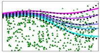
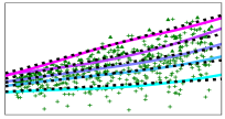
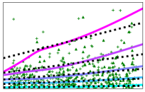
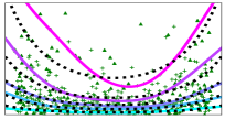
Figure 1: 1D synthetic datasets of varying functions (rows), fitted by various methods (columns). Estimated quantiles (blue through pink) compared to ground truth quantiles (dashed black lines). CQRNN recovers quantiles closest to the ground truth on most datasets.

3 Censored Quantile Regression and Neural Networks

This section considers applying the sequential grid algorithm to NNs, explaining why this is inefficient. It then describes the CQRNN algorithm, our main contribution, which avoids these pitfalls.

3.1 The Sequential Grid Algorithm and Neural Networks

To the best of our knowledge the sequential grid algorithm has been proposed and implemented only on linear models. Our first contribution is showing that, with three adjustments, it can be used in NNs.

Adj. 1) The $M$ models producing estimates, $\hat{y}_{j,\tau}$, are chosen be NNs, of any architecture with a single output. Adj. 2) While the linear version of the algorithm minimises Eq. 4 analytically with a parametric programming approach, for NNs this is instead minimised with stochastic gradient descent. Adj. 3) Portnoy [2003] proposed using a lengthy process for the first quantile. They set $\mathbf{\hat{w}}=\mathbf{1}$ and optimise Eq. 4. After optimisation, if any censored datapoints lie below the first quantile, these are removed from the dataset, and the procedure repeats until there are none. This repeated optimisation could go on for many iterations for large datasets and is costly for NNs. Instead, we simply set $\mathbf{\hat{q}}=\mathbf{0}$, and optimise the first quantile once only. We show this is roughly equivalent in Appendix A.2.

Unfortunately, this adaption is still inefficient. Inspecting Algorithm 1, one notes that $M$ NNs must be trained sequentially, meaning time complexity (both at training and at test) and memory complexity is $\mathcal{O}(M)$. This is not the case when doing quantile regression with NNs without censoring – a single NN typically uses multiple outputs, one per quantile, and their losses can be minimised simultaneously [Taylor, 2000]. For modest numbers of quantiles, this results in little overhead relative to a single NN, since the extra quantile outputs require only linear heads, while the bulk of the parameter count and computation time arise from the shared trunk of the NN.

Note that these inefficiencies are less problematic for linear models – optimisation of Eq. 4 can be performed quite rapidly, and memory complexity cannot obviously be improved beyond $\mathcal{O}(M)$. As such, it is the use of NNs that motivates the search for an alternative algorithm.

3.2 CQRNN Algorithm

Our proposed algorithm uses a single NN outputting a grid of quantile estimates that can be optimised simultaneously. This results in a more efficient algorithm in terms of training time, test time, and memory. Concretely, if the NN is a single hidden-layer NN with $H$ neurons, then the model is defined, $\psi_{\tau}(\mathbf{x}_{j},\theta)=\theta_{1,\tau}^{\intercal}\phi(\theta_{0}^{\intercal}\mathbf{x}_{i})$, with $\theta_{0}\in\mathbb{R}^{D\times H}$ shared for all estimates and $\theta_{1,\tau}\in\mathbb{R}^{H\times 1}$ for the specific output head, and non-linearity, $\phi$.

The key insight behind our algorithm is that estimates of the censored weights, $\mathbf{\hat{w}}$, can be bootstrapped from the model while it learns, without requiring sequential optimisation. Intuitively, as the model trains, the estimates of the censored quantiles, $\mathbf{\hat{q}}$, and hence the censored weights, $\mathbf{\hat{w}}$, improve, and these feedback to create a more accurate loss function, allowing further improvement of the model.

We summarise the method in Algorithm 2. The quantile of a censored datapoint is estimated as whichever NN output is closest under the current model parameters. Whilst the algorithm is written in two steps, getting up-to-date estimates of censored quantiles, $\hat{q}_{j}$, requires only a forward pass, which is done at the point of loss optimisation anyway, so actually comes ‘for free’. In our implementations, the algorithm is extended to leverage mini-batches and modern optimisers (e.g. Adam).

Algorithm 2 CQRNN algorithm.

Dataset $\mathcal{D}$, one parametric model $\psi(\cdot)$ with randomly initialised parameters $\theta$ that can output $M$ quantile predictions, quantiles to be estimated $\operatorname{grid}_{\tau}$, learning rate $\alpha$, pseudo y value $y^{*}$.

$\mathcal{S}_{\text{censored}}\leftarrow$ $\{i\in\{0,1,\dots,N\}:\Delta_{i}=0\},\mathcal{S}_{\text{observed}}\leftarrow$ $\{i\in\{0,1,\dots,N\}:\Delta_{i}=1\}$

while not convereged do

     1. Hard expectation step

     for $j\in\mathcal{S}_{\text{censored}}$ do

         $\hat{q}_{j}\leftarrow\arg\min_{\tau}|\hat{y}_{j,\tau}-y_{j}|$ $\triangleright$ Estimate quantile of censored data under current model

         $\hat{w}_{j}\leftarrow\max\left((\tau-\hat{q}_{j})/(1-\hat{q}_{j}),0\right)$ $\triangleright$ Avoid negative weights if $\hat{q}_{j}>\tau$      

     2. Partial maximisation step

     $\theta\leftarrow\theta-\alpha\partial\mathcal{L}(\theta_{\tau},\mathcal{D},\tau,\mathbf{\hat{w}},y^{*})/\partial\theta\;\;\forall\tau\in\operatorname{grid}_{\tau}$ $\triangleright$ Gradient step to minimise Eq. 4

4 Analysis of CQRNN

The previous section introduced the CQRNN algorithm, motivating it intuitively, while this section considers its correctness. Providing precise analytical guarantees is very challenging, both due to the involvement of non-convex NNs, and the bootstrapping nature of the algorithm. We therefore consider more holistic ways of understanding and providing confidence in the method. We firstly show that it can be interpreted as a flavour of EM (‘generalised hard’ EM) – connecting to this well-studied class of algorithms provides some justification of CQRNN’s design. We secondly validate the way the model bootstraps its own censored quantile estimates by describing a ‘self-correcting’ property.

4.1 Interpretation as Expectation-Maximisation

EM is a two-stage iterative optimisation technique for finding maximum likelihood solutions. It can be useful when one has both observed and latent variables, and where knowing the latent variables would allow straightforward optimisation of a model’s parameters and vice versa.

In our problem, we interpret the weights of the censored datapoints, $\mathbf{w}$, as latent variables, observed variables as $\mathbf{x}$ & $y$, and the NN parameters $\theta$ are to be optimised. Under our notation, the vanilla EM procedure [Bishop, 2006] can be written as follows (using a randomly initialising $\theta^{\text{old}}$),

1. Expectation step. Evaluate, $p(\mathbf{w}|\mathbf{x},y,\theta^{\text{old}})$, to set up the expectation,

   $$\mathcal{Q}(\theta,\theta^{\text{old}})=\int_{\mathbf{w}}p(\mathbf{w}|\mathbf{x},y,\theta^{\text{old}})\log p(y,\mathbf{w}|\mathbf{x},\theta)d\mathbf{w}=\mathbb{E}_{\mathbf{w}|\mathbf{x},y,\theta^{\text{old}}}[\log p(y,\mathbf{w}|\mathbf{x},\theta)].$$ (6)

2. Maximisation step. Perform optimisation of the expected likelihood.

   $$\theta^{\text{new}}={\arg\max}_{\theta}\mathcal{Q}(\theta,\theta^{\text{old}})$$ (7)

3. Set $\theta^{\text{old}}\leftarrow\theta^{\text{new}}$ and repeat until convergence.

We now show how our CQRNN method in Algorithm 2 can be interpreted as a flavour of EM, specifically generalised hard EM. The key steps in this interpretation are: 1) The likelihood for datapoints at each quantile are chosen to follow an asymmetric Laplace distribution. 2) The expectation step is treated as a hard assignment under the current NN parameters. 3) The likelihood is only partially maximised at each iteration.

Likelihood Form

A likelihood function is required for both the E & M steps. Theorem 1 shows how Eq. 4 can be interpreted as a negative log likelihood.

Theorem 1. Let the likelihood for each datapoint at each quantile be an asymmetric Laplace distribution with scale, $\lambda=\sqrt{\tau-\tau^{2}}$, and asymmetry, $k=\tau/\sqrt{\tau-\tau^{2}}$. The negative log likelihood is,

$$-\log p(y|\mathbf{x},\theta,\mathbf{w},y^{*}) =\sum_{\tau\in\text{grid}_{\tau}}\mathcal{L}_{\text{Port.}}(\theta,y,\mathbf{x},\tau,\mathbf{w},y^{*})+\operatorname{constant}.$$ (8)

Proof sketch. The asymmetric Laplace distribution has been used in Bayesian treatments of quantile regression without censoring [Yu and Moyeed, 2001]. We extend this to Portnoy’s loss with a weighted likelihood form using the censored weights. Appendix A provides the full proof.

Expectation as a Hard Assignment of Latent Variables

In some models, such as a Gaussian mixture model, the expectation step can be computed through analytical evaluation of the latent posterior distribution [Bishop, 2006]. In our case, $p(\mathbf{w}|\mathbf{x},y,\theta^{\text{old}})$, is intractable, though Eq. 4 depends linearly on each element $w_{j}$, so we need only consider the expectation, $\mathbb{E}_{w_{j}|\mathbf{x},y,\theta^{\text{old}}}[w_{j}]$. The algorithm can then be interpreted as making an assignment under the current model parameters,

$$\hat{\mathbb{E}}_{w_{j}|\mathbf{x}_{j},y_{j},\theta^{\text{old}}}[w_{j}] =\sum_{w_{j}}w_{j}\hat{p}(w_{j}|\mathbf{x}_{j},y_{j},\theta^{\text{old}})=\frac{\tau-\hat{q}_{j}}{1-\hat{q}_{j}},$$ (9)

$$\hat{p}(w_{j}|\mathbf{x}_{j},y_{j},\theta^{\text{old}}) =\begin{cases}1\text{ if }w_{j}=\frac{\tau-\hat{q}_{j}}{1-\hat{q}_{j}}\text{, where }\hat{q}_{j}=\arg\min_{\tau}|\hat{y}_{j,\tau}-y_{j}|\\ 0\text{ else}\end{cases}.$$ (10)

This is a ‘hard’ assignment, where latents are assigned to the most likely values under the current model (e.g. datapoints are attributed to the nearest clusters in the K-means algorithm [Bishop, 2006]), and gives rise to a class of algorithms termed hard EM [Samdani et al., 2012].

Note that the in Eq. 6 we can rewrite, $\log p(y,\mathbf{w}|\mathbf{x},\theta)=\log p(\mathbf{w})p(y|\mathbf{x},\theta,\mathbf{w})$. Since we choose only a single setting for $\mathbf{w}$ in the outer expectation, this dependence disappears, and we require maximisation of, $\mathbb{E}_{\mathbf{w}|\mathbf{x},y,\theta^{\text{old}}}[\log p(y|\mathbf{x},\theta,\mathbf{w})]$.

Partial Maximisation

A second departure from the standard EM algorithm, is that Algorithm 2 performs only a partial maximisation of the likelihood, taking a single gradient step. This has been shown to provide similar guarantees, and is termed ‘generalised’ EM [Neal and Hinton, 1998].

One could consider an alternative version of the algorithm that is closer to the standard EM procedure, where the estimated quantiles of censored data points are fixed while the maximisation step of NN parameters is run to convergence over multiple training epochs, before the estimates are updated in the expectation step, and repeating. In our case this is less effective – the maximisation requires running a forward pass through the NN, and obtaining estimated quantiles under current NN parameters once this is done is trivial, so we can access up-to-date estimates essentially for free. Appendix Figure 5 empirically demonstrates that CQRNN’s partial maximisation approach produces the fastest convergence.

4.2 Self-Correcting Property

The CQRNN bootstraps weight estimates from the current model as it trains. It’s not immediately obvious why this bootstrapping approach should converge to something sensible – what if bad initial weight estimates lead to worse ones? As a second insight into the CQRNN algorithm, Theorem 2 shows that when a censored weight, $\hat{w}_{j}$, is estimated incorrectly, the algorithm acts in a way to adjust the estimated quantiles in a favourable way – we refer to this as ‘self-correcting’.

Theorem 2. If $\hat{q}_{j}$ is underestimated, one iteration of the algorithm acts to increase the quantile predictions, $\hat{y}_{j,\tau}$, by the same amount, or even higher, than if the weight had been correct. If $\hat{q}_{j}$ is overestimated, $\hat{y}_{j,\tau}$, is decreased by the same amount, or even lower, than with the correct weight.

Proof sketch. Denote ${q}_{j}$ the true quantile that censored datapoint $j$ is censored in, and ${w}_{j}$ the corresponding true weight. We derive the expression for the gradient wrt the predicted quantiles, $\hat{y}_{j,\tau}$, finding that if $\hat{w}_{j}$ is underestimated it holds that, $\frac{\partial\mathcal{L}_{\text{Port.}}(\theta,\mathcal{D},\tau,\hat{\mathbf{w}},y^{*})}{\partial\hat{y}_{j,\tau}}\leq\frac{\partial\mathcal{L}_{\text{Port.}}(\theta,\mathcal{D},\tau,{\mathbf{w}},y^{*})}{\partial\hat{y}_{j,\tau}}$, and hence gradient descent applies an adjustment in the desired direction of equal or greater magnitude than if the true weight had been used. The reverse holds for overestimated $\hat{w}_{j}$. Appendix A provides a full proof.

5 Related Work

Survival analysis and NNs. Following the widespread success of deep NNs over the past decade, there has been a wave of research applying NNs to survival analysis – for instance by modifying the CoxPH model [Katzman et al., 2018], or framing the task as ordinal classification [Lee et al., 2018]. Closer to our work are methods that use NNs to output parameters of a distribution such as the Weibull [Martinsson, 2016], seek robust training objectives for these models [Avati et al., 2019], or help with their optimisation [Tang et al., 2022]. Our work stands out as offering a way to directly estimate the target variable at pre-specified quantiles, without enforcing any distributional assumption. A limitation is that the distribution may only be predicted at these quantiles (unless additional assumptions are made to allow interpolation between these).

Quantile regression and NNs. Quantile regression has proven an attractive option to enable NNs to move beyond point predictions. This allows quantification of a NN’s aleatoric uncertainty [Tagasovska and Lopez-Paz, 2019]. It is attractive due to its straightforward implementation, and avoidance of any distributional assumption. For example, it has found use in reinforcement learning to capture the distribution of rewards, rather than just the mean [Dabney et al., 2017]. Since NNs are flexible function approximators, particular attention has been paid to the crossing quantile problem [Bondell et al., 2010, Zhou et al., 2020, Brando et al., 2022]. CQRNN borrows ideas from this line of work, and further tackles the challenge of learning quantiles under censored data.

Censored quantile linear regression. There is much work on censored quantile regression methods for linear models. Powell [1986] developed an estimator under fixed-value censoring which can be implemented with an algorithm from Fitzenberger [1997]. Portnoy [2003] developed an estimator under random censoring based on the KM estimator, while Peng and Huang [2008] developed an alternative based on the Nelson–Aalen (NA) estimator. KM and NA are closely related, and Portnoy and Peng’s methods have been reported to offer similar empirical performance [Koenker, 2008]. Koenker [2022] provides all above methods in the popular ‘quantreg’ R package. Other notable methods include Yang et al. [2018], based on the data augmentation algorithm, and Wang and Wang [2009], whose estimator is similar to Portnoy’s but utilises local estimates of the KM, computed with a kernel method. See Peng [2021] for a review of the broader area. Our work allows modelling of flexible non-linear quantile functions, leveraging the powerful representation learning abilities of NNs. Although, this sacrifices the interpretability of coefficients of linear models.

Censored quantile regression and NNs. Only a small amount of work has been done in this area. The ‘qrnn’ R package [Cannon, 2019] offers the ability to train NNs under fixed-value left censoring, adopting an idea from the linear setting [Friederichs and Hense, 2007, Cannon, 2011]. Huttel et al. [2022] explore our objective but assume censoring times, $c_{i}$, are available for both censored and uncensored data points (i.e. the censoring distribution is known). We do not require this assumption. DeepQuantReg [Jia and Jeong, 2022] tackles the same objective as this paper. They showed that improvements in quantile estimation can be obtained relative to naive methods. Their work differs from ours significantly – they base their method around an estimator for the median from Huang et al. [2007], requiring an assumption that the censoring distribution is independent of covariates.

6 Experiments

This section empirically investigates several questions. Q1) How does the proposed CQRNN method compare with existing methods? This is done qualitatively on synthetic 1D functions in Section 6.1 and quantitatively on synthetic and real datasets in Section 6.2. Q2) How does the sequential grid algorithm compare to the CQRNN algorithm, both in terms of predictive accuracy and efficiency? Explored in Section 6.3 Q3) How is the CQRNN algorithm affected by its hyperparameters? We investigate the impact of grid fidelity and $y^{*}$ in Section 6.4.

All experiments use fully-connected NNs with two hidden layers of 100 neurons, except for SurvMNIST, when three convolutional layers are used. Grid size $M$ is set to 5, 9 or 19 depending on dataset size. Appendix B contains further details on hyperparameter settings, metrics, and datasets. Appendix C presents further results.

Datasets. We use three types of dataset. Type 1) Synthetic target data with synthetic censoring. Type 2) Real target data with synthetic censoring. Type 3) Real target data with real censoring. Whilst type 3 captures the kind of datasets we care about most, evaluation of quantiles is challenging since in real-world survival data the target conditional quantiles are not obtainable even at test time [Li and Peng, 2017]. In contrast, type 1 offers access to the ground truth quantiles for clean evaluation, but properties of these datasets may be less realistic. We introduce type 2 as a middle ground, which takes a real-world dataset without censoring, and synthetically overlays a censoring distribution to create training data. At test time, we have the option of not applying the censoring, providing samples from the clean target distribution, allowing clearer evaluation. We summarise all datasets in Table 2. Full details are in Appendix B.4. Our experiments exceed the number and variety of datasets used in popular recent works [Goldstein et al., 2020, Zhong et al., 2021]

Metrics. Our objective is to measure how closely a model’s predicted quantiles match those of the ground truth target distribution. We favour different metrics for each dataset type.

For type 1 datasets, since targets are generated synthetically it is possible to analytically compute the ground truth target quantile for an input $\mathbf{x}_{i}$, which we denote $y_{i,\tau}$. We compute the mean squared error (MSE) between the predictions and the ground truths across three quantiles, $\tau\in[0.1,0.5,0.9]$, (we ensure these are always present in $\operatorname{grid}_{\tau}$). This is our first-choice metric when available. $\text{True quantile MSE (TQMSE)}\coloneqq\frac{1}{N}\sum_{\tau\in[0.1,0.5,0.9]}\sum_{i=1}^{N}(\hat{y}_{i,\tau}-y_{i,\tau})^{2}.$

In type 2 datsets samples from the uncensored target distribution are available but not the synthetic generating function. Our preferred metric is the checkmark loss across the three quantiles. $\text{Uncensored quantile loss (UQL)}\coloneqq\frac{1}{N}\sum_{\tau\in[0.1,0.5,0.9]}\sum_{i=1}^{N}\rho_{\tau}(y_{i},\hat{y}_{i,\tau})$.

For datasets of type 3, we use two metrics. The concordance index (C-index) is computed using the median ($\tau=0.5$). But this may not reveal anything about systematic bias of different models, nor about other quantiles $\tau\neq 0.5$. We secondly use censored D-Calibration (CensDCal) [Haider et al., 2020] which measures whether the empirical proportion of datapoints falling between pairs of consecutive quantiles, matches the target proportion, $\tau_{j+1}-\tau_{j}$. MSE of the deviation is then computed. There is also an uncensored version (UnDCal), which we can compute for type 1 & 2 datasets. Appendix B.2 gives further details.

Baselines. We compare against three methods that can be used to predict the quantiles of a target distribution using a NN. Excl. Censor – a method that naively excludes censored datapoints from the training data, optimising the loss in Eq. 3. DeepQuantReg – the only existing method in the literature proposing explicit output of quantiles from a NN on censored data [Jia and Jeong, 2022]. LogNorm MLE – A NN outputting parameters of a lognormal distribution, that’s trained via maximum likelihood estimation (MLE) (details in Appendix B.3), and is a standard baseline in related work (e.g. [Avati et al., 2019, Goldstein et al., 2020]) since this distribution often suits properties of real-world time-to-event survival data [Kleinbaum and Klein, 2012].

6.1 Qualitative 1D Analysis

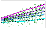
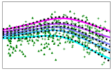
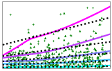
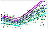
Figure 3: This figure shows estimated quantiles (blue through pink) compared to ground truth quantiles (dashed black lines). It shows 1D synthetic datasets of varying functions and noise distributions (rows), fitted by various methods (columns).

Figure 1 visualises the quantiles predicted by CQRNN and baseline methods for 1D datasets (Table 2 describes dataset functions, Figure 3 visualises further 1D datasets). Each dataset contains 500 datapoints drawn from, $\mathbf{x}\sim\mathcal{U}(0,2)$ and $\operatorname{grid}_{\tau}\in\{0.1,0.3,0.5,0.7,0.9\}$. CQRNN usually learns quantiles that are closer to the ground truth than baseline methods, particularly at higher quantiles. Excl. censor systemically makes underpredictions, and this worsens at higher quantiles since larger values of $y$ are more likely to be censored and excluded. DeepQuantReg avoids this systemic underprediction, but appears to introduce bias of its own. LogNorm MLE provides variable results – on Norm uniform it fails with excessive variance (an issue also observed by Avati et al. [2019]), but on LogNorm, since the target distribution matches the distribution output by the NN, it performs well.

Table 1: Performance of our proposed CQRNN algorithm (Algorithm 2) compared to the sequential grid method for NNs (Algorithm 1), over 200 random seeds.

Dataset	Number	Training time	Test time	Parameter	TQMSE difference	CQRNN is	Seq. grid is	No statistical
	quantiles	speed up	speed up	saving	Seq. grid $-$ CQRNN	sig. better	sig. better	significant
					95% conf. interval	in TQMSE?	in TQMSE?	difference
Norm linear	9	14.7$\times$	11.2$\times$	8.3$\times$	-2.189 $\pm$ 0.245	✓
Norm non-lin	9	12.4$\times$	9.6$\times$	8.3$\times$	-0.003 $\pm$ 0.001	✓
Exponential	9	12.4$\times$	8.0$\times$	8.3$\times$	-0.093 $\pm$ 0.176			✓
Weibull	9	12.5$\times$	8.7$\times$	8.3$\times$	-0.014 $\pm$ 0.016			✓
LogNorm	9	12.9$\times$	8.8$\times$	8.3$\times$	-0.039 $\pm$ 0.028	✓
Norm uniform	9	12.6$\times$	8.1$\times$	8.3$\times$	0.175 $\pm$ 0.033		✓
Norm heavy	19	31.0$\times$	18.5$\times$	16.2$\times$	0.108 $\pm$ 0.211			✓
Norm med.	19	34.1$\times$	17.9$\times$	16.2$\times$	-0.046 $\pm$ 0.004	✓
Norm light	19	31.7$\times$	19.2$\times$	16.2$\times$	-0.035 $\pm$ 0.003	✓
Norm same	19	34.3$\times$	21.2$\times$	16.2$\times$	-0.390 $\pm$ 0.049	✓
LogNorm heavy	19	33.6$\times$	19.9$\times$	16.2$\times$	0.005 $\pm$ 0.001		✓
LogNorm med.	19	31.3$\times$	13.1$\times$	16.2$\times$	0.019 $\pm$ 0.002		✓
LogNorm light	19	31.3$\times$	20.2$\times$	16.2$\times$	-0.033 $\pm$ 0.004	✓
LogNorm same	19	29.8$\times$	18.4$\times$	16.2$\times$	-0.371 $\pm$ 0.045	✓
Total:						8/14	3/14	3/14

Type 1 datasets

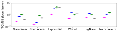
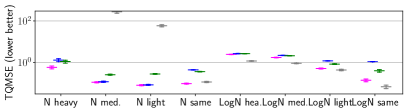
Type 2 datasets

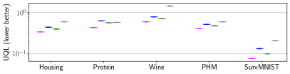
Type 3 datasets

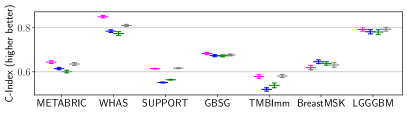
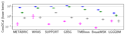
Figure 2: Main benchmarking results. Mean $\pm$ one standard error over ten runs.

6.2 Benchmarking

Our main experiment benchmarks CQRNN against all baselines across a wide variety of datasets, covering various domains, sizes, dimensionalities and censoring proportions (see Table 2). Some hyperparameter tuning was performed for each method (Appendix B.1). Figure 2 plots the preferred metric for each dataset type, though patterns were consistent across metrics – Table 4 provides a full breakdown.

For type 1 (synthetic) datasets, the quantitative results follow our qualitative observations, with CQRNN producing lowest TQMSE on all but the datasets generated from a Log Normal distribution, when it sometimes placed second behind LogNorm MLE.

CQRNN also produces the lowest UQL on all datasets of type 2. LogNorm MLE performs poorly on these, presumably since they are not typical time-to-event datasets which are well captured by the Log Normal distribution.

For type 3 datasets, CQRNN and LogNorm MLE usually perform best in terms of C-index, with error bars tending to overlap. In CensDCal, CQRNN consistently perform best, matched only by LogNorm MLE on two datasets, when error bars overlap. Excl. censor is the weakest method, with DeepQuantReg midway between it and CQRNN.

6.3 Comparison of Sequential Grid and CQRNN

We ran a head-to-head comparison of CQRNN and the sequential grid algorithm on all type 1 synthetic datasets, and all type 3 real datasets. Table 1 compares on type 1 datasets, along with statistical tests of significance for TQMSE differences (200 random seeds). Appendix Table 5 provides results for the type 3 datsets, reporting C-index and CensDCal (50 random seeds). Significance tests are described in Appendix B.1.

CQRNN delivers benefits in speed up both at training and test time, running an order of magnitude faster than the sequential grid algorithm. CQRNN also dramatically reduces model size. The magnitude of these benefits is largely determined by the size of the quantile grid, $M$, which is explicit in the sequential algorithm’s time and space complexity, $\mathcal{O}(M)$, but largely avoided in CQRNN.

Differences in the quality of quantiles of the two algorithms is usually slight (after-all both leverage the same estimator), though CQRNN shows statistically significant gains on 8/14 type 1 datasets in terms of TQMSE, 4/7 type 3 datsets in terms of C-Index, and 7/7 type 3 datasets in terms of CensDCal. We hypothesise that having a single NN output all quantiles provides a helpful inductive bias, encouraging similarity between adjacent quantiles, that’s not present in independently trained NNs.

6.4 Hyperparameter Investigation

The CQRNN algorithm includes two hyperparameters – the grid of quantiles, $\operatorname{grid}_{\tau}$, and the pseudo y value, $y^{*}$. We ran ablations to empirically investigate the effect of these, as well as remedies for the ‘crossing-quantile’ problem, and a comparison of partial vs. full optimisation. Here we summarise our findings, Appendix C.1 provides full details.

We tested grid sizes, $M\in\{9,19,39\}$, on several type 1 datasets. In general, a finer grid (larger $M$) is slightly beneficial, though there is variance between datasets and gains are sometimes only seen for larger datasets (>5,000 datapoints). Selection of $y^{*}$ requires some care for CQRNN. We defined it in terms of the maximum $y$ value in the training set, $y^{*}=c_{y^{*}}\max_{i}y_{i}$, for a hyperparemeter, $c_{y^{*}}>1$. Performance can be improved by tuning $c_{y^{*}}$ for each dataset, but using $c_{y^{*}}=1.2$ provided consistently reasonable results – this was the value used in our benchmarking experiments. We trialled two methods for combating the crossing-quantile problem. 1) Adding a crossing loss penalty. 2) Constraining the NN architecture to output quantiles adding to the previous prediction. Neither of these methods significantly affected performance.

7 Discussion & Conclusion

This paper has taken a popular idea from survival analysis, Portnoy’s censored quantile regression estimator, and shown how it can be efficiently combined with NNs in a new algorithm, CQRNN. We provided theoretical insight by interpreting it as a flavour of EM. Empirically the method outperformed existing approaches, consistently producing more accurate quantile estimates across a range of synthetic and real datasets. For example, across datasets of type 2 and 3, CQRNN was best calibrated in 10 out of 12 instances (see CensDCal in Table 4).

Limitations. Firstly, our theoretical results have not said that solutions will converge on a global optimum. Secondly, we have only tested CQRNN on a modest number of real-world datasets, many drawn from the biomedical domain. It’s possible that some datasets may cause CQRNN problems, as we found on BreastMSK (Figure 2). In particular, cases where higher quantiles are undefined should be handled with care.

Conclusion. To summarise, our work contributes toward unlocking the benefit that modern machine learning could bring to important domains such as healthcare and machinery prognostics. By outputting quantiles, CQRNN naturally communicates a measure of uncertainty in its predictions, which makes it particularly suitable to these high-stakes applications, and a valuable addition to the toolkit combining deep NNs with survival analysis.

Table 2: Summary of all datasets used.

Dataset	Feats	Train	Test	Prop.	Target sampling	Censoring sampling
		data	data	censored	distribution	distribution
Type 1 – Synthetic datasets with synthetic censoring
Norm linear	1	500	1000	0.20	$\mathcal{N}(2x+10,(x+1)^{2})$	$\mathcal{N}(4x+10,(0.8x+0.4)^{2})$
Norm non-linear	1	500	1000	0.24	$\mathcal{N}(x\sin(2x)+10,(0.5x+0.5)^{2})$	$\mathcal{N}(2x+10,2^{2})$
Exponential	1	500	1000	0.30	$\operatorname{Exp}(2x+4)$	$\operatorname{Exp}(-3x+15)$
Weibull	1	500	1000	0.22	$\operatorname{Weibull}(4x\sin(2(x-1))+10,5)$	$\operatorname{Weibull}(-3x+20,5)$
LogNorm	1	500	1000	0.21	$\operatorname{Lognorm}((x-1)^{2},x^{2})$	$\mathcal{U}(0,10)$
Norm uniform	1	500	1000	0.62	$\mathcal{N}(2x\cos(2x)+13,(x^{2}+0.5)^{2})$	$\mathcal{U}(0,18)$
Norm heavy	4	2000	1000	0.80	$\mathcal{N}(3x_{0}+x_{1}^{2}-x_{2}^{2}+2\sin(x_{2}x_{3})+6,(x^{2}+0.5)^{2})$	$\mathcal{U}(0,12)$
Norm med.	4	2000	1000	0.49	— ” —	$\mathcal{U}(0,20)$
Norm light	4	2000	1000	0.25	— ” —	$\mathcal{U}(0,40)$
Norm same	4	2000	1000	0.50	— ” —	Equal to target dist.
LogNorm heavy	8	4000	1000	0.75	$\operatorname{Lognorm}(\sum_{i}^{8}\beta_{i}x_{i},1)/10$	$\mathcal{U}(0,0.4)$
LogNorm med.	8	4000	1000	0.52	— ” —	$\mathcal{U}(0,1.0)$
LogNorm light	8	4000	1000	0.23	— ” —	$\mathcal{U}(0,3.5)$
LogNorm same	8	4000	1000	0.50	— ” —	Equal to target dist.
Type 2 – Real datasets with synthetic censoring
Housing	8	16512	4128	0.50	Real	$\mathcal{U}(0,c_{1})$
Protein	9	36584	9146	0.44	Real	$\mathcal{U}(0,c_{2})$
Wine	11	5197	1300	0.69	Real	$\mathcal{U}(0,c_{3})$
PHM	21	36734	9184	0.52	Real	$\mathcal{U}(0,c_{4})$
SurvMNIST	28$\times$28	48000	12000	0.53	One Gamma dist. per MNIST class	$\mathcal{U}(0,c_{5})$
Type 3 – Real datasets with real censoring
METABRIC	9	1523	381	0.42	Real	Real
WHAS	6	1310	328	0.57	Real	Real
SUPPORT	14	7098	1775	0.32	Real	Real
GBSG	7	1785	447	0.42	Real	Real
TMBImmuno	3	1328	332	0.49	Real	Real
BreastMSK	5	1467	367	0.77	Real	Real
LGGGBM	5	510	128	0.60	Real	Real

Checklist

1. For all authors…

   1. Do the main claims made in the abstract and introduction accurately reflect the paper’s contributions and scope? [Yes]

   2. Did you describe the limitations of your work? [Yes] See Section 7.

   3. Did you discuss any potential negative societal impacts of your work? [N/A] We don’t foresee direct negative societal impacts from our algorithm.

   4. Have you read the ethics review guidelines and ensured that your paper conforms to them? [Yes]

2. If you are including theoretical results…

   1. Did you state the full set of assumptions of all theoretical results? [Yes]

   2. Did you include complete proofs of all theoretical results? [Yes] See Appendix A.

3. If you ran experiments…

   1. Did you include the code, data, and instructions needed to reproduce the main experimental results (either in the supplemental material or as a URL)? [Yes] Code is available at https://github.com/TeaPearce/Censored_Quantile_Regression_NN.

   2. Did you specify all the training details (e.g., data splits, hyperparameters, how they were chosen)? [Yes] See Appendix B.1.

   3. Did you report error bars (e.g., with respect to the random seed after running experiments multiple times)? [Yes] Standard errors over ten random seeds are included in main results in Figure 2 and Table 4.

   4. Did you include the total amount of compute and the type of resources used (e.g., type of GPUs, internal cluster, or cloud provider)? [Yes] See Appendix B.

4. If you are using existing assets (e.g., code, data, models) or curating/releasing new assets…

   1. If your work uses existing assets, did you cite the creators? [Yes] Data details are given in Appendix B.4.

   2. Did you mention the license of the assets? [Yes] All datasets used are opensourced.

   3. Did you include any new assets either in the supplemental material or as a URL? [Yes] We don’t create new assets. Links to datasets used are provided in Appendix B.4.

   4. Did you discuss whether and how consent was obtained from people whose data you’re using/curating? [N/A]

   5. Did you discuss whether the data you are using/curating contains personally identifiable information or offensive content? [Yes] Data details are given in Appendix B.4.

5. If you used crowdsourcing or conducted research with human subjects…

   1. Did you include the full text of instructions given to participants and screenshots, if applicable? [N/A]

   2. Did you describe any potential participant risks, with links to Institutional Review Board (IRB) approvals, if applicable? [N/A]

   3. Did you include the estimated hourly wage paid to participants and the total amount spent on participant compensation? [N/A]

Appendix A Analytical Results

A.1 Proofs

Theorem 1.

Let the likelihood for each datapoint at each quantile be an asymmetric Laplace distribution with scale, $\lambda=\sqrt{\tau-\tau^{2}}$, and asymmetry, $k=\tau/\sqrt{\tau-\tau^{2}}$. The negative log likelihood is,

$$-\log p(y|\mathbf{x},\theta,\mathbf{w},y^{*}) =\sum_{\tau\in\text{grid}_{\tau}}\mathcal{L}_{\text{Port.}}(\theta,y,\mathbf{x},\tau,\mathbf{w},y^{*})+\operatorname{constant}.$$ (11)

Proof.

Define the likelihood over all quantiles of interest, and split censored datapoints into two pseudo datapoints, one at the censoring location and one at the large pseudo value $y^{*}$, to give a weighted likelihood,

$$p(y|\mathbf{x},\theta,\mathbf{w},y^{*}) =\prod_{\tau\in\text{grid}_{\tau}}p(y|\mathbf{x},\theta,\mathbf{w},y^{*},\tau),$$ (12)

$$p(y|\mathbf{x},\theta,\mathbf{w},y^{*},\tau) =\prod_{i\in\mathcal{S}_{\text{observed}}}p(y_{i}|\mathbf{x}_{i},\theta)\prod_{j\in\mathcal{S}_{\text{censored}}}p(y_{j}|\mathbf{x}_{j},\theta)^{w_{j}}p(y^{*}|\mathbf{x}_{j},\theta)^{1-w_{j}}.$$ (13)

We write the asymmetric Laplace density with $\hat{y}_{j,\tau}$ as the location parameter and scale $\lambda$ and asymmetry $k$,

$$f(y_{j};\hat{y}_{j,\tau},\lambda,k)=\frac{\lambda}{k+1/k}\begin{cases}\exp((\lambda/k)(y_{j}-\hat{y}_{j,\tau}))\;\text{ if }\;\hat{y}_{j,\tau}>y_{j}\\ \exp(-\lambda k(y_{j}-\hat{y}_{j,\tau}))\;\;\,\text{ else}\end{cases}.$$ (14)

Setting $\lambda=\sqrt{\tau-\tau^{2}}$ and $k=\tau/\sqrt{\tau-\tau^{2}}$ and rearranging,

$$f(y_{j};\hat{y}_{j,\tau},\lambda,k) =(\tau-\tau^{2})\exp(y_{j}-\hat{y}_{j,\tau})(-\tau+\mathbb{I}[\hat{y}_{j,\tau}>y_{j}])$$ (15)

$$\log f(y_{j};\hat{y}_{j,\tau},\lambda,k) =-\rho_{\tau}(y_{j},\hat{y}_{j,\tau})+\operatorname{constant}$$ (16)

Taking the logarithm of Eq. 13 we have,

$$\log p(y|\mathbf{x},\theta,\mathbf{w},y^{*}) =$$

$$\sum_{\tau\in\text{grid}_{\tau}} \sum_{i\in\mathcal{S}_{\text{observed}}}\log p(y_{i}|x_{i},\theta)+\sum_{j\in\mathcal{S}_{\text{censored}}}\log p(y_{j}|x_{j},\theta)^{w_{j}}+\log p(y^{*}|x_{j},\theta)^{1-w_{j}}.$$ (17)

Eq. 16 may be substituted into this if all likelihoods of observed and censored pseudo datapoints are chosen to follow asymmetric Laplace distributions. Taking the negative then recovers the theorem’s result.

∎

Theorem 2.

If $\hat{q}_{j}$ is underestimated, one iteration of the algorithm acts to increase the quantile predictions, $\hat{y}_{j,\tau}$, by the same amount, or even higher, than if the weight had been correct. If $\hat{q}_{j}$ is overestimated, $\hat{y}_{j,\tau}$, is decreased by the same amount, or even lower, than with the correct weight.

Remark.

Note that if a quantile $\hat{q}_{j}$ is underestimated, it’s desirable to increase the quantiles relating to that datapoint, for input $\mathbf{x}_{j}$ and predictions $\hat{y}_{j,\tau}$. If a quantile $\hat{q}_{j}$ is instead overestimated, it’s desirable to decrease the quantiles for input $\mathbf{x}_{j}$ and predictions $\hat{y}_{j,\tau}$. We refer to this desired behaviour as ‘self-correcting’.

Proof.

Denote ${q}_{j}$ the true quantile that censored datapoint $j$ is censored in, and ${w}_{j}=(\tau-{q}_{j})/(1-{q}_{j})$ the corresponding true weight. We now consider one iteration of the algorithm in the case that the estimated quantile is underestimated.

1. Model underpredicts the censored quantile, $\hat{q}_{j}={q}_{j}-\epsilon$, for some $\epsilon>0$.

2. The corresponding weight is also underestimated, $\hat{q}_{j}<{q}_{j}\implies\hat{w}_{j}<{w}_{j}$, shown in lemma 2.1.

3. Lemma 2.3 shows that, for censored datapoint $j$, the gradient of Eq. 4 wrt the quantile prediction $\hat{y}_{j,\tau}$ is,

   $$\frac{\partial\mathcal{L}_{\text{Port.}}(\theta,\mathcal{D},\tau,\mathbf{w},y^{*})}{\partial\hat{y}_{j,\tau}}=\begin{cases}-\tau&\text{ if, }\hat{y}_{j,\tau}<y_{j}\\ w_{j}-\tau&\text{ if, }y_{j}\leq\hat{y}_{j,\tau}<y^{*}\\ 1-\tau&\text{ if, }y^{*}\leq\hat{y}_{j,\tau}\\ \end{cases}.$$ (18)

   Hence, if $\hat{w}_{j}$ is underestimated it holds that, $\frac{\partial\mathcal{L}_{\text{Port.}}(\theta,\mathcal{D},\tau,\hat{\mathbf{w}},y^{*})}{\partial\hat{y}_{j,\tau}}\leq\frac{\partial\mathcal{L}_{\text{Port.}}(\theta,\mathcal{D},\tau,{\mathbf{w}},y^{*})}{\partial\hat{y}_{j,\tau}}$.

4. When this gradient is used for optimisation, this has the effect of increasing the quantile prediction, $\hat{y}_{j,\tau}$, by either the same amount, or even higher, than if the weight had been correct.

Similar (reversed) logic applies if the quantile is initially overestimated, $\hat{q}_{j}={q}_{j}+\epsilon$, (e.g. lemma 2.2) which encourages decreasing the quantile predictions, $\hat{y}_{j,\tau}$, by the same amount or lower than with correct weights. Hence, weight estimates will be improved in future iterations of the algorithm. Note that this applies to all quantiles, $\tau\in\operatorname{grid}_{\tau}$.

∎

Lemma 2.1.

Let, $\hat{q}_{j}={q}_{j}-\epsilon$, and $\epsilon>0$. It holds that, $\hat{q}_{j}<{q}_{j}\implies\hat{w}_{j}<{w}_{j}$, for, $\tau\in(0,1)$, and, $\hat{q}_{j},{q}_{j}\in(0,1)$.

Proof.

From the definition of the weights, $\hat{w}_{j}<{w}_{j}\implies(\tau-{q}_{j}-\epsilon)/(1-{q}_{j}-\epsilon)<(\tau-{q}_{j})/(1-{q}_{j})$.

Let $a\coloneqq\tau-{q}_{j}$ and $b\coloneqq 1-{q}_{j}$. Note that, $a<b$, since by assumption, $\tau<1$. We must show that,

$$\frac{a-\epsilon}{b-\epsilon} <\frac{a}{b}$$ (19)

$$\frac{a-\epsilon}{b-\epsilon}\frac{b}{a} <1$$ (20)

$$\frac{ab-b\epsilon}{ab-a\epsilon} <1,\text{ which holds since, }a<b.$$ (21)

∎

Lemma 2.2.

Let, $\hat{q}_{j}={q}_{j}+\epsilon$, and $\epsilon>0$. It holds that, $\hat{q}_{j}>{q}_{j}\implies\hat{w}_{j}>{w}_{j}$, for, $\tau\in(0,1)$, and, $\hat{q}_{j},{q}_{j}\in(0,1)$.

Proof.

This proof follows lemma 2.1. We now have,

$$\frac{ab+b\epsilon}{ab+a\epsilon} >1,\text{ which holds since, }a<b.$$ (22)

∎

Lemma 2.3.

The partial derivative of Portnoy’s loss wrt the predicted quantile, for censored datapoint $j$, is given by,

$$\frac{\partial\mathcal{L}_{\text{Port.}}(\theta,\mathcal{D},\tau,\mathbf{w},y^{*})}{\partial\hat{y}_{j,\tau}}=\begin{cases}-\tau&\text{ if, }\hat{y}_{j,\tau}<y_{j}\\ w_{j}-\tau&\text{ if, }y_{j}\leq\hat{y}_{j,\tau}<y^{*}\\ 1-\tau&\text{ if, }y^{*}\leq\hat{y}_{j,\tau}\\ \end{cases}.$$ (23)

Proof.

Recalling that,

$$\rho_{\tau}(y_{i},\hat{y}_{i,\tau})=(y_{i}-\hat{y}_{i,\tau})\left(\tau-\mathbb{I}[\hat{y}_{i,\tau}>y_{i}]\right),$$ (24)

we have,

$$\frac{\partial\rho_{\tau}(y_{i},\hat{y}_{i,\tau})}{\partial\hat{y}_{j,\tau}}=\mathbb{I}[\hat{y}_{i,\tau}>y_{i}]-\tau.$$ (25)

We are interested in the derivative for the censored portion of Portnoy’s loss in Eq. 4,

$$\frac{\partial w_{j}\rho_{\tau}(y_{j},\hat{y}_{j,\tau})+(1-w_{j})\rho_{\tau}(y^{*},\hat{y}_{j,\tau})}{\partial\hat{y}_{j,\tau}}.$$ (26)

Note that we always choose, $y^{*}>y_{j}$. Hence $\hat{y}_{j,\tau}<y_{j}\implies\hat{y}_{j,\tau}<y^{*}$, so there are three cases to consider. Case 1, $\hat{y}_{j,\tau}<y_{j}$, case 2, $y_{j}\leq\hat{y}_{j,\tau}<y^{*}$, case 3 $y^{*}\leq\hat{y}_{j,\tau}$.

For case 1,

$$\frac{\partial w_{j}\rho_{\tau}(y_{j},\hat{y}_{j,\tau})+(1-w_{j})\rho_{\tau}(y^{*},\hat{y}_{j,\tau})}{\partial\hat{y}_{j,\tau}} =w_{j}(-\tau)+(1-w_{j})(-\tau)=-\tau.$$ (28)

For case 2,

$$\frac{\partial w_{j}\rho_{\tau}(y_{j},\hat{y}_{j,\tau})+(1-w_{j})\rho_{\tau}(y^{*},\hat{y}_{j,\tau})}{\partial\hat{y}_{j,\tau}} =w_{j}(1-\tau)+(1-w_{j})(-\tau)=w_{j}-\tau.$$ (29)

For case 3,

$$\frac{\partial w_{j}\rho_{\tau}(y_{j},\hat{y}_{j,\tau})+(1-w_{j})\rho_{\tau}(y^{*},\hat{y}_{j,\tau})}{\partial\hat{y}_{j,\tau}} =w_{j}(1-\tau)+(1-w_{j})(1-\tau)=1-\tau.$$ (30)

∎

A.2 First Iteration of the Sequential Grid Algorithm

In this section we compare the procedure proposed by Portnoy [2003] to find the first quantile predicted at, $\tau_{0}\coloneqq\operatorname{grid}_{\tau}[0]$, with the procedure we propose in the sequential grid algorithm for NNs (Algorithm 1). We show that these two procedures produce equivalent gradients.

Portnoy’s procedure. Portnoy [2003] require that no censored datapoints lie below the first quantile, and propose deleting these from the dataset when this does occur, as follows.

1. Set $\mathbf{w}=\mathbf{1}$ for all censored datapoints in dataset.

2. Optimise $\mathcal{L}_{\text{Port.}}$ (Eq. 4) for $\tau_{0}$.

3. Find all censored datapoints below $\tau_{0}$, $B\leftarrow\{j\in\mathcal{S}_{\text{censored}}:y_{j}<\hat{y}_{j,\tau_{0}}\}$.

4. If $B$ is empty then exit.

5. Exclude all elements of $B$ from the dataset and repeat.

This optimisation could be repeated many times. We’d like to avoid this since training NNs on potentially large datasets can be costly.

Sequential grid for NNs procedure. Algorithm 1 instead simply sets $\mathbf{q}=\mathbf{0}$, and optimises the first quantile once only.

1. Set $\mathbf{q}=\mathbf{0}$ for all censored datapoints in dataset.

2. Optimise $\mathcal{L}_{\text{Port.}}$ (Eq. 4) for $\tau_{0}$.

Justification. We now justify why this is a reasonable approximation. First note that when $\hat{q}_{j}=0$ we have, $\hat{w}_{i}=\frac{\tau-\hat{q}_{i}}{1-\hat{q}_{i}}=\tau$. Using lemma 2.3 we can compare the gradients for each procedure.

For Portoy’s procedure, when $$\hat{w}_{j}=1$$,

$$\frac{\partial\mathcal{L}_{\text{Port.}}(\theta,\mathcal{D},\tau,\mathbf{\hat{w}},y^{*})}{\partial\hat{y}_{j,\tau}} =\begin{cases}-\tau&\text{ if, }\hat{y}_{j,\tau}<y_{j}\\ 1-\tau&\text{ if, }y_{j}\leq\hat{y}_{j,\tau}<y^{*}\implies\text{set to 0 in next iteration}\\ 1-\tau&\text{ if, }y^{*}\leq\hat{y}_{j,\tau}\\ \end{cases}.$$ (32)

For Algorithm 1, when $$\hat{q}_{j}=0$$,

$$\frac{\partial\mathcal{L}_{\text{Port.}}(\theta,\mathcal{D},\tau,\mathbf{\hat{w}},y^{*})}{\partial\hat{y}_{j,\tau}} =\begin{cases}-\tau&\text{ if, }\hat{y}_{j,\tau}<y_{j}\\ 0&\text{ if, }y_{j}\leq\hat{y}_{j,\tau}<y^{*}\\ 1-\tau&\text{ if, }y^{*}\leq\hat{y}_{j,\tau}\\ \end{cases}.$$ (33)

At first look, the gradients appear to differ in the case $y_{j}\leq\hat{y}_{j,\tau}<y^{*}$. But when a datapoint triggers this criteria in Portnoy’s procedure, it will be excluded and the model retrained, in which case its gradient becomes 0. As such the gradients for a censored datapoint in both procedures are equivalent.

Appendix B Experimental Details

This section provides further details about all experiments run. Our code base uses the $\operatorname{PyTorch}$ framework. Hyperparameters in Appendix B.1. Metrics in Appendix B.2. Baselines in Appendix B.3. Datasets in Appendix B.4.

Hardware. We used an internal cluster for experiments, utilising machines with four GPUs and 14 CPU cores. Most of our datasets used fully-connected NNs, which were trained on CPU, while GPUs were used for the SurvMNIST experiments.

B.1 Full Hyperparameter Details

Below we list hyperparameter settings used and where applicable the tuning protocols followed.

B.1.1 Qualitative 1D Analysis

Section 6.1 experiment. All methods used the same optimisation procedure and NN architecture, without tuning.

• Training dataset size: 500, where, $\mathbf{x}\sim\mathcal{U}(0,2)$

• Epochs: 100

• Optimiser: Adam

• Learning rate: 0.01 (decreased 70% and 90% of the way through training)

• Batch size: 128

• Weight decay: 0.0001

• NN architecture: Fully-connected, two hidden layers of 100 hidden nodes, GeLU activations

• $y^{*}=1.2\times\max_{i}y_{i}$

• $\operatorname{grid}_{\tau}\in\{0.1,0.3,0.5,0.7,0.9\}$

B.1.2 Benchmarking

Section 6.2 experiment. Experiments were repeated over 10 random seeds. Hyperparameter settings.

• Training dataset size: various – see Table 2

• Test dataset size: various – see Table 2

• Epochs: $\in\{10,20,50,100\}$

• Optimiser: Adam

• Learning rate: 0.01 for fc NN, 0.001 for CNN (decreased 70% and 90% of the way through training)

• Batch size: 128

• Weight decay: 0.0001

• Default NN architecture: Fully-connected, two hidden layers of 100 hidden nodes, ReLU activations

• CNN architecture for SurvMNIST following Goldstein et al. [2020]: Conv2D[64, (5$\times$5)] $\to$ ReLU $\to$ Dropout(0.2) $\to$ AveragePool(2$\times$2) $\to$ Conv2D[128, (5$\times$5)] $\to$ ReLU $\to$ Dropout(0.2) $\to$ AveragePool(2$\times$2) $\to$ Conv2D[256, (2$\times$2)] $\to$ ReLU $\to$ Linear

• $y^{*}=1.2\times\max_{i}y_{i}$

• Grid size $M\in\{6,10,20\}$

• Dropout $\in\{\operatorname{True},\operatorname{False}\}$

Tuning process for epochs and dropout:

• For the real type 2 and type 3 datasets, we tuned number of epochs $\in\{10,20,50,100\}$ and dropout $\in\{\operatorname{True},\operatorname{False}\}$ for each dataset for each method. We used three random splits as a validation (but not overlapping with the random seeds used in the final test run).

• Epochs was fixed to 100 and dropout disabled for: Norm linear, Norm non-linear, Exponential, Weibull, LogNorm, Norm uniform.

• Epochs was fixed to 20 and dropout disabled for: Norm heavy, Norm medium, Norm light, Norm same.

• Epochs was fixed to 10 and dropout disabled for: LogNorm heavy, LogNorm medium, LogNorm light, LogNorm same.

We fixed the grid size according to an estimate of how densely the datapoints covered the input space (a rough consideration of dataset size and number of features):

• Grid size $M=5$ for smaller datasets with more features: WHAS, SUPPORT, GBSG, TMBImmuno, BreastMSK, LGGGBM, METABRIC.

• Grid size $M=9$ for medium datasets or smaller datasets with less features: Norm linear, Norm non-linear, Exponential, Weibull, LogNorm, Norm uniform.

• Grid size $M=19$ for larger datasets or those with less features: Norm heavy, Norm medium, Norm light, Norm same, LogNorm heavy, LogNorm medium, LogNorm light, LogNorm same, Housing, Protein, Wine, PHM, SurvMNIST.

B.1.3 Comparison of Sequential Grid and CQRNN

Section 6.3 experiment. This was carried out under the same protocol as for the main benchmarking, but repeated over a larger number of seeds (200 for type 1 datasets, 50 for type 3 datasets). To obtain 95% confidence intervals, we compute the standard error of the difference between means, and multiply it by a two-sided t-statistic, with (number of seeds$-1$) degrees of freedom at the $\alpha=0.05$ significance level. If zero falls within this confidence interval, the difference is deemed not significant.

B.1.4 Hyperparameter Investigation

Section 6.4 experiment. Hyperparameters are as for the main benchmarking except $M$ and $y^{*}$ were varied as stated in the text. Epochs were set via the formula epochs $=500\times 200/N$ ensuring the same number of gradient updates were made on each run. Experiments were repeated over 100 random seeds for the grid investigation, and ten random seeds for the $y^{*}$ investigation.

B.2 Metrics

This section briefly expands upon the metrics introduced in Section 6. Table 3 summarises the availability on each metric for each dataset type. The computation of each is also detailed below.

Table 3: Availability of metrics for each dataset type.

Dataset type	Target distribution	Censoring distribution	TQMSE	UQL	UnDCal	CensDCal	C-Index
Type 1	Synthetic	Synthetic	✓	✓	✓	✓	✓
Type 2	Real	Synthetic	✗	✓	✓	✓	✓
Type 3	Real	Real	✗	✗	✗	✓	✓

True quantile MSE (TQMSE) $$\coloneqq\frac{1}{N}\sum_{\tau\in[0.1,0.5,0.9]}\sum_{i=1}^{N}(\hat{y}_{i,\tau}-y_{i,\tau})^{2}$$ (34)

Uncensored quantile loss (UQL) $$\coloneqq\frac{1}{N}\sum_{\tau\in[0.1,0.5,0.9]}\sum_{i=1}^{N}\rho_{\tau}(y_{i},\hat{y}_{i,\tau})$$ (35)

Uncensored D-Calibration (UnDCal) $$\coloneqq 100\times\sum_{j=1}^{M-1}\left(\left(\tau_{j+1}-\tau_{j}\right)-\frac{1}{N}\sum_{i=1}^{N}\mathbb{I}[\hat{y}_{i,\tau_{j}}<y_{i}\leq\hat{y}_{i,\tau_{j+1}}]\right)^{2}$$ (36)

Censored D-Calibration (CensDCal) $$\coloneqq 100\times\sum_{j=1}^{M-1}\left(\left(\tau_{j+1}-\tau_{j}\right)-\frac{1}{N}\xi\right)^{2}$$ (37)

where, Goldstein et al. [2020] defines,

$$\xi=\sum_{i\in\mathcal{S}_{\text{observed}}}\mathbb{I}[\hat{y}_{i,\tau_{j}}<y_{i}\leq\hat{y}_{i,\tau_{j+1}}]+ \sum_{i\in\mathcal{S}_{\text{censored}}}\frac{(\tau_{j+1}-q_{i})\mathbb{I}[\hat{y}_{i,\tau_{j}}<y_{i}\leq\hat{y}_{i,\tau_{j+1}}]}{1-q_{i}}+\frac{(\tau_{j+1}-\tau_{j})\mathbb{I}[q_{i}<\tau_{j}]}{1-q_{i}}.$$ (38)

We increase the magnitude of DCal metrics by $100\times$ to make the numbers of similar order to TQMSE and UQL.

B.3 Baselines

This section provides some extra detail about the LogNorm MLE baseline. For this method, we use a NN with two outputs, representing the mean, $\mu$, and standard deviation, $\sigma$, of a Log Normal distribution, i.e. $\log y\sim\mathcal{N}(\hat{\mu},\hat{\sigma}^{2})$. We pass the output representing the standard deviation prediction through a $\operatorname{SoftPlus}$ to ensure it is always positive and differentiable.

The maximum likelihood estimation loss is then,

$$-\mathcal{L}_{\text{MLE}}(\theta,\mathcal{D})\coloneqq\sum_{i\in\mathcal{S}_{\text{observed}}}\log p(y_{i}|\mathbf{x}_{i},\theta)+\sum_{j\in\mathcal{S}_{\text{censored}}}\log(1-\operatorname{CDF}(y_{j}|\mathbf{x}_{j},\theta)),$$ (39)

where the likelihood and CDF follow the analytical expressions for the Log Normal distribution. At evaluation time, we use the $\operatorname{SciPy}$ package to compute the quantiles from the predicted Log Normal distribution that correspond to those in $\operatorname{grid}_{\tau}$. This allows a like-for-like comparison with our other baselines.

B.4 Dataset Details

This section provides further detail about the source of each dataset used. All real-world datasets were taken from open-access repositories, and had already been anonymised. For real-world datasets, we do not follow any previous test/train splits, rather we randomly shuffle the data for each run, selecting 80% for training and 20% for testing.

B.4.1 Type 1 Datasets

Table 2 details the generating target and censoring distributions used, as well as numbers of test and train datapoints. Inputs were always generated uniformly via, $\mathbf{x}\sim\mathcal{U}(0,2)^{D}$ for $D$ features.

B.4.2 Type 2 Datasets

Table 2 details dataset sizes and number of features. All datasets used a uniform censoring distribution, $c_{i}\sim\mathcal{U}(0,c)$, where $c$ was selected to be equal to the 90th percentile of the target distribution for SurvMNIST, and $c=1.5\max_{i}y_{i}$ for the other type 2 datasets. Housing was sourced from Scikit Learn datasets, while Protein, Wine and PHM were sourced through OpenML https://www.openml.org/.

• Housing Target is median house prices. Retrieved from https://scikit-learn.org/stable/datasets/real_world.html#california-housing-dataset.

• Protein Target is RMSD. OpenML lookup ID is physicochemical-protein.

• Wine Target is quality of wine. OpenML lookup ID is wine quality.

• PHM (prognostics health management) target is breakdown time of simulated machines. OpenML lookup ID is NASA PHM2008.

Our final type 2 dataset is slightly different, since we don’t use the provided labels directly.

• SurvMNIST appeared in Goldstein et al. [2020], who adapted it from Sebastian Pölsterl’s blog: https://k-d-w.org/blog/2019/07/survival-analysis-for-deep-learning/. It uses the standard MNIST dataset http://yann.lecun.com/exdb/mnist/, but targets are drawn from a Gamma distribution, with different parameters per class. Goldstein et al. [2020] used a small variance fixed across classes, with means $\in[11.25,2.25,5.25,5.0,4.75,8.0,2.0,11.0,1.75,10.75]$. For our purposes, we are most interested in how well methods capture variance, so we vary it, variance $\in[0.1,0.5,0.1,0.2,0.2,0.2,0.3,0.1,0.4,0.6]$.

B.4.3 Type 3 Datasets

We provide a brief overview of each dataset. Four datasets – GBSG, METABRIC, SUPPORT, WHAS – were all retrieved from https://github.com/jaredleekatzman/DeepSurv/tree/master/experiments/data. Katzman et al. [2018] provides a detailed introduction to these datasets. The other three datasets – TMBImmnuo, BreastMSK, LGGGBM – were all sourced from the cBioPortal, https://www.cbioportal.org/, for cancer genomics.

• GBSG (Rotterdam & German Breast Cancer Study Group) requires prediction of survival time for breast cancer patients.

• METABRIC (Molecular Taxonomy of Breast Cancer International Consortium) requires prediction of survival time for breast cancer patients. Covariates include expressions for four genes as well as clinical data.

• SUPPORT (Study to Understand Prognoses Preferences Outcomes and Risks of Treatment) requires prediction of survival time in seriously ill hospitalised patients. Covariates include demographic and basic diagnosis information.

• WHAS (Worcester Heart Attack Study) requires prediction of acute myocardial infraction survival.

• TMBImmuno (Tumor Mutational Burden and Immunotherapy) requires prediction of survival time for patients with various cancer types using clinical data. Covariates include age, sex, and number of mutations. Retrieved from https://www.cbioportal.org/study/clinicalData?id=tmb_mskcc_2018.

• BreakMSK requires prediction of survival time for patients with breast cancer using tumour information. Covariates include ER, HER, HR, mutation count, TMB. Retrieved from https://www.cbioportal.org/study/clinicalData?id=breast_msk_2018.

• LGGGBM. requires prediction of survival time for cancer patient from clinical data. Covariates include age, sex, purity, mutation count, TMB. Retrieved from https://www.cbioportal.org/study/clinicalData?id=lgggbm_tcga_pub

Appendix C Further Results

CQRNN            Sequential grid            Excl. censor            DeepQuantReg           LogNorm MLE

Table 4: Full results table for all datasets, methods and metrics. Mean $\pm$ 1 standard error for test set over 10 runs.

Dataset	Method	MSE to true quantile	Uncensored quantile loss	Uncensored D-Calibration	Concordance-Index	Censored D-Calibration
		(lower better)	(lower better)	(lower better)	(higher better)	(lower better)
	Type 1 – synthetic data, synthetic censoring
Norm linear	CQRNN	0.088 $\pm$ 0.009	1.517 $\pm$0.01	0.327 $\pm$0.057	0.663 $\pm$0.002	0.211 $\pm$0.034
Norm linear	Sequential grid	2.779 $\pm$ 0.506	1.623 $\pm$0.02	0.303 $\pm$0.06	0.662 $\pm$0.002	0.224 $\pm$0.024
Norm linear	Excl. censor	0.566 $\pm$ 0.039	1.62 $\pm$0.016	3.078 $\pm$0.244	0.662 $\pm$0.002	2.349 $\pm$0.102
Norm linear	DeepQuantReg	1.172 $\pm$ 0.133	1.695 $\pm$0.026	1.94 $\pm$0.192	0.663 $\pm$0.002	1.241 $\pm$0.138
Norm linear	LogNorm MLE	0.184 $\pm$ 0.021	1.522 $\pm$0.008	0.315 $\pm$0.023	0.662 $\pm$0.002	0.232 $\pm$0.04
Norm non-lin	CQRNN	0.028 $\pm$ 0.004	0.759 $\pm$0.005	0.262 $\pm$0.044	0.674 $\pm$0.004	0.186 $\pm$0.023
Norm non-lin	Sequential grid	0.027 $\pm$ 0.003	0.759 $\pm$0.005	0.283 $\pm$0.034	0.673 $\pm$0.004	0.194 $\pm$0.03
Norm non-lin	Excl. censor	0.053 $\pm$ 0.004	0.768 $\pm$0.006	0.579 $\pm$0.088	0.673 $\pm$0.004	0.449 $\pm$0.054
Norm non-lin	DeepQuantReg	0.818 $\pm$ 0.093	0.998 $\pm$0.019	4.263 $\pm$0.234	0.609 $\pm$0.023	2.593 $\pm$0.206
Norm non-lin	LogNorm MLE	0.323 $\pm$ 0.035	0.824 $\pm$0.009	1.651 $\pm$0.118	0.653 $\pm$0.005	0.971 $\pm$0.077
Exponential	CQRNN	1.298 $\pm$ 0.201	4.057 $\pm$0.04	0.404 $\pm$0.035	0.559 $\pm$0.003	0.248 $\pm$0.031
Exponential	Sequential grid	1.702 $\pm$ 0.397	4.061 $\pm$0.039	0.391 $\pm$0.057	0.558 $\pm$0.004	0.226 $\pm$0.025
Exponential	Excl. censor	11.03 $\pm$ 0.772	4.456 $\pm$0.039	2.537 $\pm$0.18	0.535 $\pm$0.007	1.513 $\pm$0.14
Exponential	DeepQuantReg	20.046 $\pm$ 5.844	4.675 $\pm$0.09	2.294 $\pm$0.252	0.544 $\pm$0.004	1.276 $\pm$0.158
Exponential	LogNorm MLE	17.825 $\pm$ 2.831	4.342 $\pm$0.058	1.056 $\pm$0.071	0.552 $\pm$0.003	0.401 $\pm$0.045
Weibull	CQRNN	0.255 $\pm$ 0.025	1.879 $\pm$0.018	0.33 $\pm$0.037	0.772 $\pm$0.002	0.211 $\pm$0.023
Weibull	Sequential grid	0.261 $\pm$ 0.018	1.877 $\pm$0.017	0.352 $\pm$0.037	0.772 $\pm$0.002	0.209 $\pm$0.023
Weibull	Excl. censor	2.468 $\pm$ 0.118	2.18 $\pm$0.021	1.942 $\pm$0.152	0.769 $\pm$0.002	0.834 $\pm$0.069
Weibull	DeepQuantReg	1.116 $\pm$ 0.16	2.005 $\pm$0.037	1.057 $\pm$0.159	0.769 $\pm$0.002	0.556 $\pm$0.126
Weibull	LogNorm MLE	1.586 $\pm$ 0.081	2.048 $\pm$0.02	0.603 $\pm$0.036	0.771 $\pm$0.002	0.478 $\pm$0.072
LogNorm	CQRNN	0.411 $\pm$ 0.057	1.716 $\pm$0.04	0.253 $\pm$0.025	0.59 $\pm$0.004	0.161 $\pm$0.015
LogNorm	Sequential grid	0.328 $\pm$ 0.036	1.716 $\pm$0.041	0.28 $\pm$0.033	0.591 $\pm$0.003	0.193 $\pm$0.024
LogNorm	Excl. censor	1.757 $\pm$ 0.114	1.818 $\pm$0.051	1.46 $\pm$0.129	0.588 $\pm$0.004	1.119 $\pm$0.062
LogNorm	DeepQuantReg	1.279 $\pm$ 0.168	1.843 $\pm$0.04	1.924 $\pm$0.131	0.58 $\pm$0.004	1.279 $\pm$0.106
LogNorm	LogNorm MLE	0.247 $\pm$ 0.032	1.713 $\pm$0.041	0.115 $\pm$0.014	0.589 $\pm$0.004	0.151 $\pm$0.018
Norm uniform	CQRNN	0.388 $\pm$ 0.054	1.442 $\pm$0.022	2.219 $\pm$0.212	0.789 $\pm$0.003	0.094 $\pm$0.008
Norm uniform	Sequential grid	0.188 $\pm$ 0.016	1.409 $\pm$0.017	1.347 $\pm$0.136	0.788 $\pm$0.003	0.462 $\pm$0.02
Norm uniform	Excl. censor	1.088 $\pm$ 0.112	1.501 $\pm$0.018	1.557 $\pm$0.19	0.79 $\pm$0.003	0.721 $\pm$0.066
Norm uniform	DeepQuantReg	2.591 $\pm$ 0.56	1.809 $\pm$0.084	4.397 $\pm$0.687	0.598 $\pm$0.064	0.418 $\pm$0.074
Norm uniform	LogNorm MLE	939.992 $\pm$ 144.76	7.727 $\pm$0.502	32.486 $\pm$1.405	0.77 $\pm$0.006	4.259 $\pm$0.144
Norm heavy	CQRNN	0.579 $\pm$ 0.089	0.999 $\pm$0.041	6.491 $\pm$1.094	0.922 $\pm$0.002	0.301 $\pm$0.067
Norm heavy	Sequential grid	0.597 $\pm$ 0.081	0.996 $\pm$0.037	6.595 $\pm$1.406	0.923 $\pm$0.002	0.198 $\pm$0.014
Norm heavy	Excl. censor	1.285 $\pm$ 0.205	1.223 $\pm$0.069	8.206 $\pm$1.895	0.923 $\pm$0.002	0.261 $\pm$0.021
Norm heavy	DeepQuantReg	1.099 $\pm$ 0.175	1.166 $\pm$0.06	6.681 $\pm$1.365	0.923 $\pm$0.002	0.191 $\pm$0.016
Norm heavy	LogNorm MLE	5568.886 $\pm$ 1737.861	17.077 $\pm$2.442	21.283 $\pm$1.057	0.852 $\pm$0.008	1.113 $\pm$0.102
Norm med.	CQRNN	0.11 $\pm$ 0.007	0.789 $\pm$0.006	0.633 $\pm$0.138	0.896 $\pm$0.001	0.157 $\pm$0.054
Norm med.	Sequential grid	0.16 $\pm$ 0.009	0.799 $\pm$0.005	0.474 $\pm$0.046	0.895 $\pm$0.001	0.159 $\pm$0.011
Norm med.	Excl. censor	0.117 $\pm$ 0.008	0.792 $\pm$0.005	0.247 $\pm$0.02	0.896 $\pm$0.001	0.136 $\pm$0.015
Norm med.	DeepQuantReg	0.255 $\pm$ 0.016	0.847 $\pm$0.008	0.944 $\pm$0.098	0.892 $\pm$0.001	0.232 $\pm$0.029
Norm med.	LogNorm MLE	276.276 $\pm$ 41.622	3.974 $\pm$0.228	17.969 $\pm$0.548	0.865 $\pm$0.004	4.612 $\pm$0.134
Norm light	CQRNN	0.079 $\pm$ 0.005	0.778 $\pm$0.005	0.173 $\pm$0.021	0.882 $\pm$0.001	0.084 $\pm$0.008
Norm light	Sequential grid	0.117 $\pm$ 0.005	0.784 $\pm$0.004	0.352 $\pm$0.027	0.882 $\pm$0.001	0.19 $\pm$0.018
Norm light	Excl. censor	0.083 $\pm$ 0.005	0.779 $\pm$0.005	0.159 $\pm$0.017	0.882 $\pm$0.001	0.112 $\pm$0.013
Norm light	DeepQuantReg	0.277 $\pm$ 0.013	0.854 $\pm$0.008	1.205 $\pm$0.081	0.878 $\pm$0.001	0.588 $\pm$0.046
Norm light	LogNorm MLE	58.503 $\pm$ 6.922	2.475 $\pm$0.093	13.713 $\pm$0.465	0.861 $\pm$0.003	7.74 $\pm$0.286
Norm same	CQRNN	0.094 $\pm$ 0.005	0.785 $\pm$0.003	0.19 $\pm$0.022	0.893 $\pm$0.001	0.052 $\pm$0.007
Norm same	Sequential grid	0.779 $\pm$ 0.16	0.847 $\pm$0.009	0.45 $\pm$0.054	0.891 $\pm$0.001	0.102 $\pm$0.012
Norm same	Excl. censor	0.435 $\pm$ 0.01	0.927 $\pm$0.007	4.096 $\pm$0.251	0.894 $\pm$0.001	1.398 $\pm$0.07
Norm same	DeepQuantReg	0.357 $\pm$ 0.013	0.893 $\pm$0.009	3.334 $\pm$0.325	0.891 $\pm$0.001	0.983 $\pm$0.091
Norm same	LogNorm MLE	0.114 $\pm$ 0.008	0.787 $\pm$0.004	0.187 $\pm$0.024	0.894 $\pm$0.001	0.059 $\pm$0.006
LogNorm heavy	CQRNN	2.424 $\pm$ 0.055	1.123 $\pm$0.021	22.493 $\pm$0.36	0.782 $\pm$0.005	0.036 $\pm$0.004
LogNorm heavy	Sequential grid	2.42 $\pm$ 0.055	1.121 $\pm$0.021	21.938 $\pm$0.299	0.781 $\pm$0.005	0.044 $\pm$0.002
LogNorm heavy	Excl. censor	2.654 $\pm$ 0.061	1.247 $\pm$0.021	35.43 $\pm$0.629	0.772 $\pm$0.005	4.806 $\pm$0.226
LogNorm heavy	DeepQuantReg	2.639 $\pm$ 0.06	1.236 $\pm$0.022	34.132 $\pm$0.719	0.771 $\pm$0.005	3.884 $\pm$0.201
LogNorm heavy	LogNorm MLE	1.17 $\pm$ 0.052	0.868 $\pm$0.018	0.135 $\pm$0.014	0.766 $\pm$0.005	0.074 $\pm$0.008
LogNorm med.	CQRNN	1.713 $\pm$ 0.049	0.923 $\pm$0.02	5.054 $\pm$0.174	0.754 $\pm$0.004	0.064 $\pm$0.005
LogNorm med.	Sequential grid	1.699 $\pm$ 0.047	0.921 $\pm$0.02	4.968 $\pm$0.181	0.754 $\pm$0.004	0.098 $\pm$0.014
LogNorm med.	Excl. censor	2.168 $\pm$ 0.053	1.067 $\pm$0.021	12.124 $\pm$0.34	0.749 $\pm$0.004	2.586 $\pm$0.071
LogNorm med.	DeepQuantReg	2.087 $\pm$ 0.056	1.033 $\pm$0.02	10.081 $\pm$0.255	0.748 $\pm$0.003	1.373 $\pm$0.055
LogNorm med.	LogNorm MLE	0.907 $\pm$ 0.05	0.824 $\pm$0.018	0.103 $\pm$0.016	0.75 $\pm$0.003	0.07 $\pm$0.009
LogNorm light	CQRNN	0.506 $\pm$ 0.028	0.764 $\pm$0.019	0.331 $\pm$0.026	0.729 $\pm$0.003	0.135 $\pm$0.01
LogNorm light	Sequential grid	0.532 $\pm$ 0.029	0.767 $\pm$0.018	0.517 $\pm$0.04	0.729 $\pm$0.003	0.21 $\pm$0.014
LogNorm light	Excl. censor	1.185 $\pm$ 0.037	0.852 $\pm$0.02	1.518 $\pm$0.124	0.729 $\pm$0.003	0.655 $\pm$0.047
LogNorm light	DeepQuantReg	0.831 $\pm$ 0.036	0.804 $\pm$0.019	0.912 $\pm$0.061	0.726 $\pm$0.003	0.438 $\pm$0.028
LogNorm light	LogNorm MLE	0.432 $\pm$ 0.034	0.767 $\pm$0.018	0.095 $\pm$0.015	0.729 $\pm$0.002	0.079 $\pm$0.004
LogNorm same	CQRNN	0.137 $\pm$ 0.021	0.735 $\pm$0.015	0.236 $\pm$0.021	0.751 $\pm$0.002	0.055 $\pm$0.007
LogNorm same	Sequential grid	0.422 $\pm$ 0.054	0.753 $\pm$0.016	0.463 $\pm$0.046	0.752 $\pm$0.003	0.101 $\pm$0.018
LogNorm same	Excl. censor	1.068 $\pm$ 0.043	0.861 $\pm$0.019	4.112 $\pm$0.264	0.752 $\pm$0.002	1.306 $\pm$0.046
LogNorm same	DeepQuantReg	0.394 $\pm$ 0.057	0.763 $\pm$0.016	1.301 $\pm$0.265	0.748 $\pm$0.002	0.335 $\pm$0.072
LogNorm same	LogNorm MLE	0.067 $\pm$ 0.013	0.73 $\pm$0.015	0.114 $\pm$0.013	0.754 $\pm$0.002	0.052 $\pm$0.005

Dataset	Method	MSE to true quantile	Uncensored quantile loss	Uncensored D-Calibration	Concordance-Index	Censored D-Calibration
		(lower better)	(lower better)	(lower better)	(higher better)	(lower better)
	Type 2 – real data, synthetic censoring
Housing	CQRNN	-	0.34 $\pm$0.002	0.793 $\pm$0.03	0.897 $\pm$0.0	0.02 $\pm$0.004
Housing	Excl. censor	-	0.443 $\pm$0.005	2.176 $\pm$0.057	0.895 $\pm$0.001	0.311 $\pm$0.011
Housing	DeepQuantReg	-	0.399 $\pm$0.004	2.474 $\pm$0.066	0.902 $\pm$0.001	0.196 $\pm$0.031
Housing	LogNorm MLE	-	0.6 $\pm$0.002	2.794 $\pm$0.022	0.881 $\pm$0.001	1.035 $\pm$0.015
Protein	CQRNN	-	0.435 $\pm$0.001	0.275 $\pm$0.008	0.847 $\pm$0.001	0.027 $\pm$0.001
Protein	Excl. censor	-	0.631 $\pm$0.002	3.45 $\pm$0.053	0.838 $\pm$0.001	1.075 $\pm$0.02
Protein	DeepQuantReg	-	0.568 $\pm$0.002	2.809 $\pm$0.059	0.831 $\pm$0.001	0.495 $\pm$0.011
Protein	LogNorm MLE	-	0.579 $\pm$0.002	0.694 $\pm$0.018	0.817 $\pm$0.002	0.298 $\pm$0.007
Wine	CQRNN	-	0.6 $\pm$0.005	0.908 $\pm$0.069	0.815 $\pm$0.002	0.046 $\pm$0.005
Wine	Excl. censor	-	0.791 $\pm$0.005	6.606 $\pm$0.209	0.799 $\pm$0.003	0.722 $\pm$0.038
Wine	DeepQuantReg	-	0.717 $\pm$0.005	3.211 $\pm$0.159	0.792 $\pm$0.003	0.212 $\pm$0.021
Wine	LogNorm MLE	-	1.454 $\pm$0.022	5.736 $\pm$0.163	0.747 $\pm$0.004	0.784 $\pm$0.022
PHM	CQRNN	-	0.408 $\pm$0.001	0.243 $\pm$0.012	0.902 $\pm$0.001	0.008 $\pm$0.001
PHM	Excl. censor	-	0.519 $\pm$0.002	3.852 $\pm$0.037	0.901 $\pm$0.001	0.481 $\pm$0.006
PHM	DeepQuantReg	-	0.479 $\pm$0.002	1.589 $\pm$0.057	0.897 $\pm$0.001	0.154 $\pm$0.011
PHM	LogNorm MLE	-	0.599 $\pm$0.002	2.26 $\pm$0.018	0.9 $\pm$0.001	0.538 $\pm$0.007
SurvMNIST	CQRNN	-	0.076 $\pm$0.0	0.308 $\pm$0.023	0.899 $\pm$0.001	0.224 $\pm$0.005
SurvMNIST	Excl. censor	-	0.133 $\pm$0.002	2.115 $\pm$0.086	0.896 $\pm$0.001	0.512 $\pm$0.014
SurvMNIST	DeepQuantReg	-	0.1 $\pm$0.001	1.021 $\pm$0.051	0.9 $\pm$0.001	0.264 $\pm$0.013
SurvMNIST	LogNorm MLE	-	0.209 $\pm$0.001	4.348 $\pm$0.049	0.894 $\pm$0.001	0.806 $\pm$0.015
	Type 3 – real data, real censoring
METABRIC	CQRNN	-	-	-	0.644 $\pm$0.006	0.189 $\pm$0.057
METABRIC	Excl. censor	-	-	-	0.615 $\pm$0.005	7.54 $\pm$0.478
METABRIC	DeepQuantReg	-	-	-	0.601 $\pm$0.006	2.393 $\pm$0.211
METABRIC	LogNorm MLE	-	-	-	0.636 $\pm$0.006	0.72 $\pm$0.106
WHAS	CQRNN	-	-	-	0.85 $\pm$0.005	1.089 $\pm$0.431
WHAS	Excl. censor	-	-	-	0.785 $\pm$0.006	9.391 $\pm$0.709
WHAS	DeepQuantReg	-	-	-	0.774 $\pm$0.008	6.71 $\pm$0.448
WHAS	LogNorm MLE	-	-	-	0.81 $\pm$0.005	0.817 $\pm$0.139
SUPPORT	CQRNN	-	-	-	0.615 $\pm$0.002	0.179 $\pm$0.022
SUPPORT	Excl. censor	-	-	-	0.552 $\pm$0.002	9.606 $\pm$0.231
SUPPORT	DeepQuantReg	-	-	-	0.564 $\pm$0.002	6.747 $\pm$0.176
SUPPORT	LogNorm MLE	-	-	-	0.617 $\pm$0.002	2.384 $\pm$0.143
GBSG	CQRNN	-	-	-	0.683 $\pm$0.005	0.339 $\pm$0.033
GBSG	Excl. censor	-	-	-	0.673 $\pm$0.005	11.732 $\pm$0.512
GBSG	DeepQuantReg	-	-	-	0.673 $\pm$0.005	8.998 $\pm$0.479
GBSG	LogNorm MLE	-	-	-	0.677 $\pm$0.004	0.793 $\pm$0.08
TMBImmuno	CQRNN	-	-	-	0.579 $\pm$0.008	0.201 $\pm$0.04
TMBImmuno	Excl. censor	-	-	-	0.52 $\pm$0.008	9.479 $\pm$0.386
TMBImmuno	DeepQuantReg	-	-	-	0.539 $\pm$0.011	4.827 $\pm$0.306
TMBImmuno	LogNorm MLE	-	-	-	0.581 $\pm$0.007	0.634 $\pm$0.067
BreastMSK	CQRNN	-	-	-	0.619 $\pm$0.01	0.08 $\pm$0.012
BreastMSK	Excl. censor	-	-	-	0.646 $\pm$0.008	4.546 $\pm$0.235
BreastMSK	DeepQuantReg	-	-	-	0.638 $\pm$0.008	3.0 $\pm$0.17
BreastMSK	LogNorm MLE	-	-	-	0.631 $\pm$0.01	0.521 $\pm$0.058
LGGGBM	CQRNN	-	-	-	0.792 $\pm$0.008	0.372 $\pm$0.074
LGGGBM	Excl. censor	-	-	-	0.782 $\pm$0.01	2.166 $\pm$0.303
LGGGBM	DeepQuantReg	-	-	-	0.781 $\pm$0.011	1.275 $\pm$0.184
LGGGBM	LogNorm MLE	-	-	-	0.793 $\pm$0.008	0.367 $\pm$0.083

Table 5: Results comparing CQRNN and sequential grid algorithm on the type 3 datasets, real target data with real censoring. Experiments were repeated over 50 random seeds.

Raw Results, mean $\pm$ one standard error Dataset Method TQMSE UQL UnDCal Concordance-Index (higher better) Censored D-Calibration (lower better) METABRIC CQRNN - - - 0.643 $\pm$0.003 0.218 $\pm$0.026 METABRIC Sequential grid - - - 0.648 $\pm$0.002 0.399 $\pm$0.04 WHAS CQRNN - - - 0.86 $\pm$0.002 0.721 $\pm$0.091 WHAS Sequential grid - - - 0.852 $\pm$0.002 5.038 $\pm$0.74 SUPPORT CQRNN - - - 0.614 $\pm$0.001 0.159 $\pm$0.01 SUPPORT Sequential grid - - - 0.613 $\pm$0.001 0.723 $\pm$0.024 GBSG CQRNN - - - 0.678 $\pm$0.002 0.361 $\pm$0.024 GBSG Sequential grid - - - 0.678 $\pm$0.002 0.789 $\pm$0.042 TMBImmuno CQRNN - - - 0.571 $\pm$0.003 0.207 $\pm$0.021 TMBImmuno Sequential grid - - - 0.572 $\pm$0.003 0.375 $\pm$0.028 BreastMSK CQRNN - - - 0.618 $\pm$0.005 0.085 $\pm$0.01 BreastMSK Sequential grid - - - 0.597 $\pm$0.006 0.227 $\pm$0.016 LGGGBM CQRNN - - - 0.784 $\pm$0.004 0.397 $\pm$0.039 LGGGBM Sequential grid - - - 0.781 $\pm$0.004 0.491 $\pm$0.041

Difference in means, alongside 95% confidence interval Dataset Number Training time Test time Parameter C-Index difference CQRNN is CensDCal difference CQRNN is quantiles speed up speed up saving Seq. grid - CQRNN sig. better? Seq. grid - CQRNN sig. better? (>0 favours CQRNN) (<0 favours CQRNN) METABRIC 5 5.3$\times$ 2.5$\times$ 4.6$\times$ -0.005 $\pm$ 0.001 ✗ -0.181 $\pm$ 0.032 ✓ WHAS 5 5.1$\times$ 3.9$\times$ 4.6$\times$ 0.008 $\pm$ 0.001 ✓ -4.317 $\pm$ 0.745 ✓ SUPPORT 5 5.1$\times$ 2.7$\times$ 4.6$\times$ 0.001 $\pm$ 0.000 ✓ -0.564 $\pm$ 0.022 ✓ GBSG 5 5.3$\times$ 5.1$\times$ 4.6$\times$ -0.001 $\pm$ 0.000 ✗ -0.428 $\pm$ 0.026 ✓ TMBImmuno 5 5.1$\times$ 4.3$\times$ 4.6$\times$ -0.000 $\pm$ 0.001 – -0.168 $\pm$ 0.025 ✓ BreastMSK 5 5.1$\times$ 5.0$\times$ 4.6$\times$ 0.021 $\pm$ 0.004 ✓ -0.141 $\pm$ 0.018 ✓ LGGGBM 5 5.4$\times$ 5.1$\times$ 4.6$\times$ 0.003 $\pm$ 0.001 ✓ -0.094 $\pm$ 0.038 ✓ CQRNN better: 4/7 7/7 Seq grid better: 2/7 0/7 No sig. difference: 1/7 0/7

Norm linear            Norm uniform            Norm non-linear

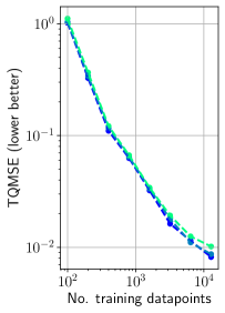
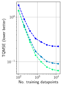
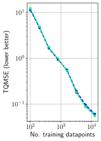
Exponential                  Weibull                  LogNorm

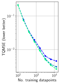
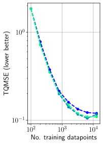
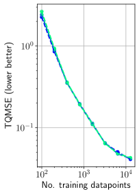
Figure 4: Ablations over grid size and number of datapoints for various synthetic datasets using our CQRNN method.

C.1 Hyperparameter ablations

The requirements for CQRNN in Algorithm 2 include two hyperparameters unique to CQRNN (the rest determine the NN and its optimisation) – the grid of quantiles, $\operatorname{grid}_{\tau}$, and the large pseudo y value, $y^{*}$. This section investigates the role of these. It also discusses two modifications which were tested in initial experiments but which were not deemed essential for good performance, and excluded from the proposed method – mitigating crossing quantiles and interpolating between quantiles.

Grid size. For evenly spaced grids, as considered in this work, the number of quantiles estimated, $M$, fully determines the grid. One might expect that a larger grid size, with finer increments between quantiles, would lead to a better fit, since censored weights can be estimated more accurately. Indeed, the convergence rate of Portnoy’s estimator was found to depend on grid size, $\mathcal{O}(1/(MN))$ [Neocleous et al., 2006].

We hypothesised that a larger grid might only deliver benefit when the dataset was sufficiently large for these fine-grained quantiles to be distinguished. Hence, Figure 4 shows an ablation investigating the interaction between grid size and number of datapoints for each of our type 1 synthetic 1D functions. Experiments were repeated with 100 random seeds, which was required to reduce the error bars sufficiently for comparison. Grid size was varied, $M\in\{9,19,39\}$, and number of datapoints, $N\in\{100,200,400,800,1600,3200,6400,12800\}$.

For all datasets and grid sizes, TQMSE decreases with dataset size. In general a larger grid size does produce lower TQMSE, and in three datasets the benefit is significant (Norm uniform, Exponential, Weibull), with the advantage indeed more pronounced with a larger dataset size. In two datasets (Norm non-linear, LogNorm), this benefit is slight, and a larger grid is even seen to be slightly harmful on very small datasets. One dataset (Norm linear) does not follow this trend, where the widest grid proves slightly harmful across all dataset sizes.

Pseudo y value. Portnoy [2003] proposed that $y^{*}$ could be set to any large value approximating $\infty$, with the R package ‘quantreg’ setting $y^{*}=1e6$. Since the sequential grid algorithm learns quantiles sequentially, it can simply halt if it attempts to estimate a quantile for which only censored datapoints remain, and hence is undefined.

The CQRNN algorithm changes this situation in two ways. Firstly, since the algorithm is no longer sequential and learns all quantiles simultaneously, it does not have the option of halting. Secondly, since a non-linear function is learnt, it is possible that higher quantiles might be undefined in one region of the input space, whilst being learnable in the rest of the space. Regressing towards an arbitrarily large $y^{*}$ value for a portion of the input space could adversely impact the quantile estimate elsewhere. When all quantiles in $\operatorname{grid}_{\tau}$ are fully defined, the effect is no different to using $\infty$.

To accommodate these differences, we recommend setting $y^{*}$ to a more modest value. We define it in terms of the maximum $y$ value in the training set, $y^{*}=c_{y^{*}}\max_{i}y_{i}$, for a hyperparemeter, $c_{y^{*}}>1$. In real-world problems, a practitioner might use an estimate for this based on their knowledge about the maximum feasible value for the target. In lieu of that, we set $c_{y^{*}}=1.2$ for all our experiments (except the below ablation!), which provided reasonable results across datasets.

Table 6 presents an ablation on four of our (multidimensional) type 1 synthetic datasets, using $c_{y^{*}}\in\{1.0,1.2,1.5,2.0,10,9,100.0\}$. For dataset Norm light, $y^{*}$ has no impact since the target distribution is fully defined under censoring. However, other datasets have input regions where the higher quantiles are not defined due to censoring, and hence higher quantiles are impacted by the magnitude of $y^{*}$. The optimal value varies by dataset (e.g. $1.2$ is best for Norm heavy, while $10.0$ is best for LogNorm heavy).

Table 6: Ablation over psuedo y value, $y^{*}$. Mean over ten runs, all hyperparameters fixed.

	—– Target value for pseudo-datapoints, $y^{*}$ —–
Dataset	$1.0\max_{i}y_{i}$	$1.2\max_{i}y_{i}$	$1.5\max_{i}y_{i}$	$2.0\max_{i}y_{i}$	$10.0\max_{i}y_{i}$	$100.0\max_{i}y_{i}$
	TQMSE (lower better)
Norm heavy	1.452	0.579	1.237	6.196	591.257	57421.824
Norm light	0.081	0.079	0.081	0.081	0.081	0.081
LogNorm heavy	2.502	2.424	2.321	2.173	1.026	19.827
LogNorm light	0.614	0.506	0.385	0.252	0.147	0.147

Crossing quantiles. One issue often discussed in quantile regression is ‘crossing quantiles’. Higher quantiles should always produce higher predictions, i.e. $\hat{y}_{i,{\tau_{1}}}>\hat{y}_{i,{\tau_{2}}}\forall\tau_{1}>\tau_{2}$. The crossing quantile issue arises when this condition does not hold. We anticipated that the flexibility of NNs might exacerbate this issue, and we tested two methods to remedy this. 1) Adding a crossing penalty to the loss [Bondell et al., 2010], $\mathcal{L}_{\text{cross}}=\sum_{i=1}^{N}\sum_{j=1}^{N_{\tau}-1}\max[0,c-(\hat{y}_{i,\text{grid}_{\tau}[j+1]}-\hat{y}_{i,\text{grid}_{\tau}[j]})]$, where $c$ is the smallest acceptable distance between neighbouring quantiles. 2) Modifying the NN architecture to enforce monotonicity between quantiles, by constraining each consecutive quantile prediction to add on to the previous one, after passing through a $\operatorname{SoftPlus}$. In our experiments, neither method significantly impacted performance. Favouring simplicity, we propose the CQRNN algorithm without these. It’s possible that other methods might have more effect, e.g. [Zhou et al., 2020, Brando et al., 2022]. We leave further exploration to future work.

Interpolating quantiles. The CQRNN algorithm sets the estimated censored quantiles, $\mathbf{q}$, by choosing the prediction closest to the censored datapoint, $\hat{q}_{j}\leftarrow\arg\min_{\tau}|\hat{y}_{j,\tau}-y_{j}|$. In early experiments, we considered an alternative approach that took a linear interpolation between the two nearest quantiles. In initial experiments this wasn’t found to significantly improve performance, so we propose the CQRNN algorithm using the simpler $\arg\min$ approach.

Partial vs. full optimisation. Figure 5 explores the effect of optimising the NNs partially, as is proposed in CQRNN in Algorithm 2, compared to fully, as might be done more typically in EM procedures. The figure shows that convergence is fastest when using partial maximisation, when the most up-to-date estimates of $\hat{q}_{i}$ are used. This ends up being more efficient than freezing $\hat{q}_{i}$ and only updating after a longer period of optimisation.

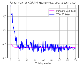
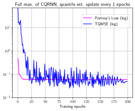
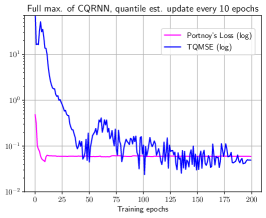
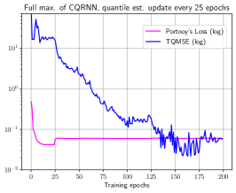
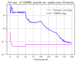
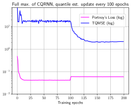
Figure 5: This figure explores the effect of optimising the NNs partially compared to fully. It shows training loss and TQMSE over training epochs. The Normal Linear dataset was used.

References

- Avati et al. [2019] Anand Avati, Tony Duan, Sharon Zhou, Kenneth Jung, Nigam H. Shah, and Andrew Y. Ng. Countdown regression: Sharp and calibrated survival predictions. 35th Conference on Uncertainty in Artificial Intelligence, UAI 2019, 2019.
- Bishop [2006] Christopher M Bishop. Pattern Recognition and Machine Learning. Springer, 2006. ISBN 9788578110796. doi: 10.1017/CBO9781107415324.004.
- Bondell et al. [2010] Howard D. Bondell, Brian J. Reich, and Huixia Wang. Noncrossing quantile regression curve estimation. Biometrika, 97:825–838, 2010. ISSN 00063444. doi: 10.1093/biomet/asq048.
- Brando et al. [2022] Axel Brando, Joan Gimeno, José Rodríguez-Serrano, and Jordi Vitrì. Deep non-crossing quantiles through the partial derivative. AISTATS, 2022.
- Cannon [2011] Alex J. Cannon. Quantile regression neural networks: Implementation in r and application to precipitation downscaling. Computers and Geosciences, 2011. ISSN 00983004. doi: 10.1016/j.cageo.2010.07.005.
- Cannon [2019] Alex J. Cannon. Quantile regression neural network ‘qrnn’. R Package, 2019. doi: 10.1016/j.cageo.2010.07.005>and.
- Dabney et al. [2017] Will Dabney, Mark Rowland, Marc G. Bellemare, and Rémi Munos. Distributional reinforcement learning with quantile regression. AAAI, 10 2017. URL http://arxiv.org/abs/1710.10044.
- Fitzenberger [1997] Bernd Fitzenberger. A guide to censored quantile regressions. Handbook of Statistics, 15:405–437, 1997. ISSN 01697161. doi: 10.1016/S0169-7161(97)15017-9.
- Friederichs and Hense [2007] P. Friederichs and A. Hense. Statistical downscaling of extreme precipitation events using censored quantile regression. Monthly Weather Review, 135:2365–2378, 2007. ISSN 0027-0644. doi: 10.1175/MWR3403.1. URL http://journals.ametsoc.org/doi/abs/10.1175/MWR3403.1.
- Goldstein et al. [2020] Mark Goldstein, Xintian Han, Aahlad Puli, Adler J. Perotte, and Rajesh Ranganath. X-cal: Explicit calibration for survival analysis. Advances in Neural Information Processing Systems, 2020. ISSN 10495258.
- Haider et al. [2020] Humza Haider, Bret Hoehn, Sarah Davis, and Russell Greiner. Effective ways to build and evaluate individual survival distributions. Journal of Machine Learning Research, 21:1–63, 2020. ISSN 15337928.
- Huang et al. [2007] Jian Huang, Shuangge Ma, and Huiliang Xie. Least absolute deviations estimation for the accelerated failure time model. Statistica, Sinica, pages 1–23, 2007.
- Huttel et al. [2022] Frederik Boe Huttel, Inon Peled, Filipe Rodrigues, and Francisco C. Pereira. Modeling censored mobility demand through censored quantile regression neural networks. IEEE Transactions on Intelligent Transportation Systems, 11 2022. ISSN 15580016. doi: 10.1109/TITS.2022.3190194.
- Jia and Jeong [2022] Yichen Jia and Jong Hyeon Jeong. Deep learning for quantile regression under right censoring: Deepquantreg. Computational Statistics and Data Analysis, 165, 2022. ISSN 01679473. doi: 10.1016/j.csda.2021.107323. URL https://doi.org/10.1016/j.csda.2021.107323.
- Katzman et al. [2018] Jared L. Katzman, Uri Shaham, Alexander Cloninger, Jonathan Bates, Tingting Jiang, and Yuval Kluger. Deepsurv: Personalized treatment recommender system using a cox proportional hazards deep neural network. BMC Medical Research Methodology, 18:1–15, 2018. ISSN 14712288. doi: 10.1186/s12874-018-0482-1.
- Kleinbaum and Klein [2012] David Kleinbaum and Mitchel Klein. Survival Analysis: A Self-Learning Text. Springer, third edition, 2012.
- Koenker [2008] Roger Koenker. Censored quantile regression redux. Journal of Statistical Software, 27:1–25, 2008. ISSN 15487660. doi: 10.18637/jss.v027.i06.
- Koenker [2022] Roger Koenker. Quantile regression, ’quantreg’. R Package, 2022. doi: 10.1017/CBO9780511754098.
- Koenker and Bassett [1978] Roger Koenker and Gilbert Bassett. Regression quantiles. Econometrica, 46:33–50, 1978.
- Lee et al. [2018] Changhee Lee, William R Zame, Jinsung Yoon, and Mihaela Van Der Schaar. Deephit: A deep learning approach to survival analysis with competing risks. AAAI, 2018. URL http://medianetlab.ee.ucla.edu/papers/AAAI_2018_DeepHit.
- Li and Peng [2017] Ruosha Li and Limin Peng. Assessing quantile prediction with censored quantile regression models. Biometrics., 2017. doi: 10.1111/biom.12627.Assessing.
- Martinsson [2016] Egil Martinsson. Wtte-rnn : Weibull time to event recurrent neural network. Master’s Thesis, 2016.
- Neal and Hinton [1998] Radford M. Neal and Geoffrey E. Hinton. A view of the em algorithm that justifies incremental, sparse, and other variants. Learning in Graphical Models, 1998.
- Neocleous et al. [2006] Tereza Neocleous, Karlien Vanden Branden, and Stephen Portnoy. Correction to censored regression quantiles by s. portnoy, 98 (2003), 1001–1012. Journal of the American Statistical Association, 101:860–861, 2006. ISSN 1537274X. doi: 10.1198/016214506000000087.
- Peng [2021] Limin Peng. Quantile regression for survival data. Annual Review of Statistics and Its Application, 8:413–437, 2021. ISSN 2326831X. doi: 10.1146/annurev-statistics-042720-020233.
- Peng and Huang [2008] Limin Peng and Yijian Huang. Survival analysis with quantile regression models. Journal of the American Statistical Association, 103:637–649, 2008. ISSN 01621459. doi: 10.1198/016214508000000355.
- Portnoy [2003] Stephen Portnoy. Censored regression quantiles. Journal of the American Statistical Association, 98:1001–1012, 2003. URL http://www.jstor.org/stable/30045346http://about.jstor.org/terms.
- Powell [1986] James L. Powell. Censored regression quantiles. Journal of Econometrics, 32:143–155, 1986. ISSN 03044076. doi: 10.1016/0304-4076(86)90016-3.
- Samdani et al. [2012] Rajhans Samdani, Ming Wei Chang, and Dan Roth. Unified expectation maximization. NAACL HLT 2012 - 2012 Conference of the North American Chapter of the Association for Computational Linguistics: Human Language Technologies, Proceedings of the Conference, 2012.
- Tagasovska and Lopez-Paz [2019] Natasa Tagasovska and David Lopez-Paz. Single-model uncertainties for deep learning. NeurIPS, 2019. URL http://arxiv.org/abs/1811.00908.
- Tang et al. [2022] Weijing Tang, Jiaqi Ma, Qiaozhu Mei, and Ji Zhu. Soden: A scalable continuous-time survival model through ordinary differential equation networks. JMLR, 8 2022. URL http://arxiv.org/abs/2008.08637.
- Taylor [2000] James W Taylor. A quantile regression neural network approach to estimating the conditional density of multiperiod returns. Journal of Forecasting, 19:299–311, 2000.
- Wang and Wang [2009] Huixia Judy Wang and Lan Wang. Locally weighted censored quantile regression. Journal of the American Statistical Association, 104:1117–1128, 2009. ISSN 01621459. doi: 10.1198/jasa.2009.tm08230. URL https://doi.org/10.1198/jasa.2009.tm08230.
- Yang et al. [2018] Xiaorong Yang, Naveen Naidu Narisetty, and Xuming He. A new approach to censored quantile regression estimation. Journal of Computational and Graphical Statistics, 27:417–425, 2018. ISSN 15372715. doi: 10.1080/10618600.2017.1385469.
- Yu and Moyeed [2001] Keming Yu and Rana A Moyeed. Bayesian quantile regression. Statistics and Probability Letters, 54:437–447, 2001.
- Zhong et al. [2021] Qixian Zhong, Jonas Mueller, and Jane-Ling Wang. Deep extended hazard models for survival analysis. NeurIPS, 2021.
- Zhou et al. [2020] Fan Zhou, Jianing Wang, and Xingdong Feng. Non-crossing quantile regression for deep reinforcement learning. NeurIPS, 2020.